
Carlos Fernando Castillo-García a, b, Juan J. Morrone c, Isaías Hazarmabeth Salgado-Ugarte a, David Espinosa a, *
a Universidad Nacional Autónoma de México, Facultad de Estudios Superiores Zaragoza, Batalla del 5 de mayo s/n, Ejército de Oriente Zona Peñón, Iztapalapa, 09230 Ciudad de México, Mexico
b Universidad Nacional Autónoma de México, Posgrado en Ciencias Biológicas, Unidad de Posgrado, Edificio D, 1er. Piso, Circuito de Posgrados, Ciudad Universitaria, Coyoacán, 04510 Ciudad de México, Mexico
c Universidad Nacional Autónoma de México, Facultad de Ciencias, Departamento de Biología Evolutiva, Museo de Zoología “Alfonso L. Herrera”, Circuito Exterior s/n, Ciudad Universitaria, Coyoacán, 04510 Ciudad de México, Mexico
*Corresponding author: despinos@unam.mx (D. Espinosa)
Received: 22 January 2024; accepted: 25 February 2025
Abstract
A software program for undertaking track analysis named Panbiotracks is introduced. It aims to solve various issues that currently are present in similar software packages. Panbiotracks is intended: 1) to be a fast, accurate, and reliable tool to generate individual tracks, generalized tracks and panbiogeographical nodes; 2) to solve the dependency on old and obsolete software that other packages have; and 3) to be a free and open source program that can be used in a variety of environments and that can be updated, modified, and improved continuously.
Keywords: Panbiogeography; Track analysis; Python; Software; Systematics
Panbiotracks: programa para análisis de trazos
Resumen
Se presenta un programa para llevar a cabo el análisis de trazos llamado Panbiotracks. Su objetivo es resolver varios problemas que están presentes en paquetes de software similares. Panbiotracks intenta: 1) ser una herramienta rápida, precisa y confiable para generar trazos individuales, trazos generalizados y nodos panbiogeográficos; 2) resolver la dependencia en software anticuado y obsoleto que tienen otros paquetes; y 3) ser un programa libre y de código abierto que pueda ser utilizado en una variedad de entornos y que puede ser actualizado, modificado y mejorado continuamente.
Palabras clave: Panbiogeografía; Análisis de trazos; Python; Software; Sistemática
Introduction
Biological evolution is closely linked to geological history. In the second half of the past century, León Croizat developed a new theoretical approach that he called “panbiogeography”. According to panbiogeography, the geographical distribution of taxa is mainly influenced by geological changes that lead to vicariance processes, where geographical barriers are the main cause of biota fragmentation, which in turn leads to speciation (Morrone, 2015).
Track analysis is panbiogeography’s primary methodological tool (Craw, 1988; Morrone, 2015). It is based on the spatial congruence between tracks, which are geometrical representations of taxon distribution. The 3 components of track analysis are individual tracks, generalized tracks, and panbiogeographical nodes (Morrone, 2015; Page, 1987). An individual track (Fig. 1a-d) is the basic unit of a panbiogeographical analysis, and is defined as an open, non-cyclic graph, also known as a minimum spanning tree (MST), whose vertices represent the geographical locations of the taxon, and the edges are the shortest paths that connect each of them. Mathematically speaking, it is a graph with n localities that are connected through n-1 edges, and whose total length is the shortest possible (Page, 1987). It can be thought of as a graphical representation of the main coordinates of a taxon in space. The basic method to draw an individual track consists of selecting a random locality and linking it to the nearest one using a straight line, then connecting both to another one, also the nearest, and repeating these steps until all the localities are connected, but without any loop between any of them. The most straightforward way to automate this is by building an adjacency matrix to find the edges, then saving the track to a file. However, some difficulty arises when measuring the distances between points, because this needs to be done considering the shape of the earth. There are multiple methods to do this, which are explained with more detail in the Algorithms subsection.
A generalized track (Fig. 1e) is a graph built from the statistically significant superposition between 2 or more individual tracks from different taxa, and it represents the history of ancestral biotas that were fragmented in the past (Craw, 1988; Morrone, 2015). However, there isn’t a formalized implementation of this concept, resulting in multiple methods that can be used to quantify it, like Parsimony Analysis of Endemicity (PAE) (Morrone, 2014; Rosen, 1988), Track Compatibility Analysis (Craw, 1988, 1989), or geometrical methods. A major issue is the difficulty of automating the process to find the generalized tracks, since the superposition between individual tracks cannot be calculated easily. Some programs, like MartiTracks (Echeverría-Londoño & Miranda-Esquivel, 2011), have approached the problem from a purely geometrical standpoint, using distances between segments to decide whether they are congruent with each other or not, but the results have not been satisfactory (Ferrari et al., 2013). The software Trazos2004 (Rojas-Parra, 2007) also uses a geometrical method, where the program finds the intersections between individual tracks and builds a generalized track from those intersections. This method does not follow the formal definition of a generalized track, since it considers only the superpositions between tracks and ignores those cases where 2 segments may be very close to each other, but without overlapping, which could also be considered as spatial congruence (Zunino & Zullini, 2003; Morrone, 2015). Even then, this method is fast and can be used to get an overall congruence approximation, since in many cases the generalized tracks obtained will reflect a general degree of similarity between individual tracks. To differentiate this approach from others, we opted to refer to the generalized tracks obtained by this method as “internal generalized tracks” (IGT).
A panbiogeographical node (Fig. 1f), marked by the superposition between the terminal segments of 2 or more generalized tracks, indicates the location of a complex area of tectonic or biotic convergence (Craw, 1988; Morrone, 2015); however, this concept may have multiple interpretations. Heads (2004) mentions that a node might represent the location of endemism, high diversity, distribution boundaries, areas of disjunction and “anomalous” absences, but also states that there are more meanings to it than these. One problem arises from the existing ways to quantify a node. As mentioned, a node is located at the ends of a generalized track, or more specifically, where 2 terminal vertices (those that are connected only to another vertex) from different generalized tracks overlap. However, other authors had considered the intersections between individual tracks, or the intersections between non-terminal segments of 2 or more generalized tracks, as nodes (Grehan, 2001; Henderson, 1989). Morrone (2015) mentions that, to avoid confusion, the former might be called “individual nodes” and the latter “generalized nodes”. In this regard, panbiogeographical nodes can be considered as a subset of generalized nodes, since the latter accounts for all the intersections between generalized tracks, while the former takes into account only those that occur at the terminal segments of generalized tracks. This means that a tool that finds generalized nodes can be used to find panbiogeographical nodes, if only those that fulfill the proper definition will be counted. Out of the 3 concepts, nodes have received the least attention from a computational point of view, possibly because the process to limit the search of the intersections between tracks to only those that happen at the terminal segments has not been properly explored.
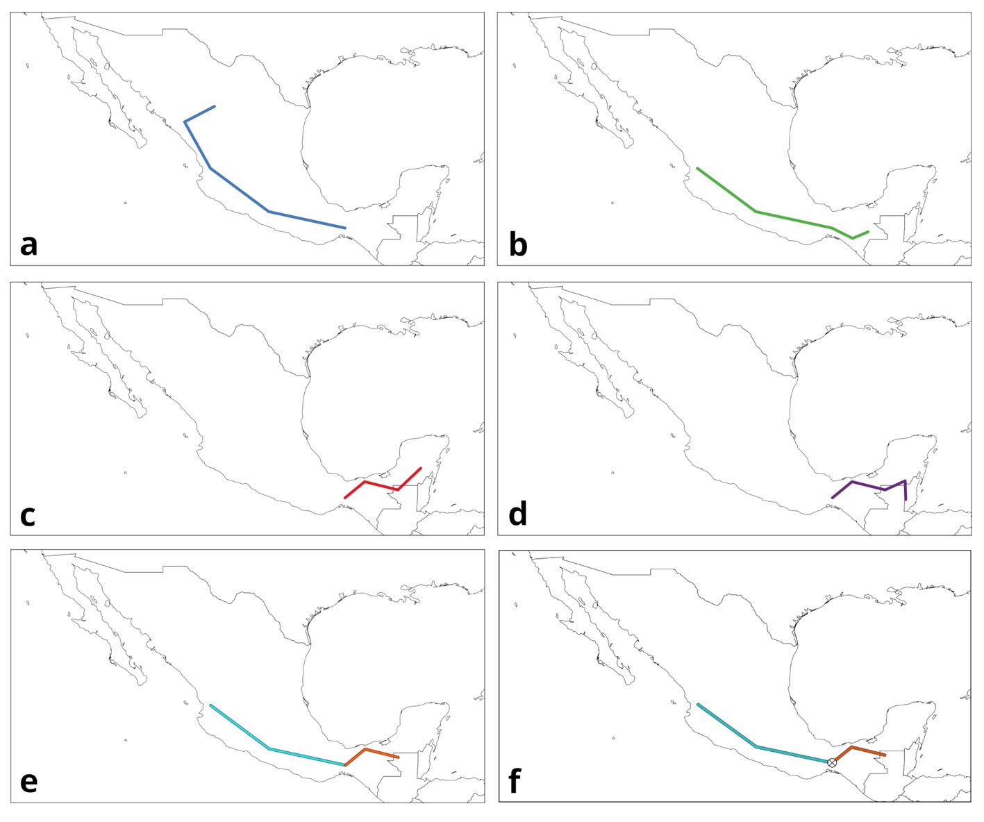
Figure 1. Panbiogeography’s main components. a-d) Individual tracks; e) generalized tracks; f) panbiogeographical node. Maps by CF Castillo-García.
The usefulness of panbiogeography and track analysis has been questioned many times, mainly regarding its ability to generate meaningful results about the evolution of species through space and time (Seberg, 1986; Waters et al., 2013). Others have criticized how track analysis is done, like the criteria used for track orientation (Seberg, 1986), or the lack of a true quantitative process to obtain generalized tracks and nodes (Ferrari et al., 2013). However, many studies have used the panbiogeographical method to identify distributional patterns of many taxa, like mammals (Escalante et al., 2018; Florentin et al., 2016), mollusks (Aguilar-Estrada & Morrone, 2022; López et al., 2022), plants (García-Díaz et al., 2023; Puga-Jiménez et al., 2013), birds (Beauchamp, 1989), fungi (González-Ávila et al., 2017), arthropods (Maya-Martínez et al., 2011), and fossil taxa (Gallo et al., 2013; Hernández-Cisneros & Vélez-Juarbe, 2021). The ability to detect ancestral biotas through generalized tracks and nodes has been mentioned by other researchers and panbiogeography has also been considered useful from other points of view, such as searching for areas of biological complexity like areas of endemism and priority conservation areas (Craw et al., 1999; Escalante et al., 2018; Miguel-Talonia & Escalante, 2013; Morrone, 2015). Because of this, we consider that the development and improvement of new methods and tools for track analysis are important and should be continued.
In recent times, several software packages have been published to automate track analysis using different algorithms and programming languages to calculate both the MSTs and the superposition between tracks and nodes. Some of them, like Trazos2004 (Rojas-Parra, 2007), Croizat (Cavalcanti, 2009), and fossil (Vavrek, 2011), use Prim’s algorithm (Sedgewick & Wayne, 2011). PASSaGE (Rosenberg & Anderson, 2011) uses its own algorithm, while SAM (Rangel et al., 2010) and MartiTracks (Echeverría-Londoño & Miranda-Esquivel, 2011) do not specify which algorithm they use. A list of the aforementioned software packages and the algorithms used by each is presented in Table 1. These programs, however, suffer from one or various of several issues: lack of documentation about what internal methods or algorithms they use, lack of accuracy in their results (Escalante et al., 2017, 2018), dependency on obsolete and unsupported software, difficulty in obtaining or reviewing their source code to improve or modify it, and lack of support for different operating systems other than Microsoft Windows and, sometimes, Apple macOS.
Table 1
Comparison between different software packages for performing track analysis and their algorithms.
| Program | Algorithms used | Measuring distance method | Platform |
| Croizat | Prim (1957), Bron and Kerbosch (1973), Wormwald (1984) | Not specified | Windows, macOS, Linux |
| Fossil | Not specified | Not specified | Independent |
| MartiTracks | Proprietary | Not specified | Windows, Linux |
| PASSaGE | Proprietary | Proprietary | Windows, macOS, Linux |
| SAM | Not specified | Not specified | Windows |
| Trazos2004 | Prim (1957) | Bessel formulae | Windows |
Panbiotracks
Panbiotracks is a Python program for track analysis that aims to overcome some of the issues mentioned above, namely the accuracy of results, dependency on obsolete software, analysis speed, and portability between operating systems. Panbiotracks addresses these issues in the following manner: 1) Accuracy and speed, by using an improved set of functions, Panbiotracks generates results in a shorter time and in more accurately than its predecessors. Moreover, since its code is smaller and is based on modern tool kits, it can be updated and improved faster than other solutions. 2) Dependency on obsolete software, since Panbiotracks uses modern releases of the Python programming language and its code is constantly reviewed to ensure that it can be used with newer versions, it is guaranteed that it will not be made obsolete in the short term. Additionally, its code can be ported to future versions of Python more easily. 3) Portability and compatibility, releases of Panbiotracks are published currently for the Windows and Linux operating systems, and a version for macOS is planned. Moreover, its source code is available publicly, which allows anyone to download it and build their own executable.
Technical information
Panbiotracks is programmed in the Python programming language version 3. It consists of one main command-line executable that can be configured at runtime to do different analyses by passing a flag that enables a particular function. Current functions are: -m I flag, generates individual tracks from a list of taxon names and localities, established by their geographical coordinates (latitude and longitude), and saves them to an ESRI shape file (SHP); -m P flag, generates an internal generalized track (IGT) from a set of individual tracks. It identifies the intersections between individual tracks and it marks the associated coordinates, then builds a new track based on those coordinates and saves it to an ESRI shape file (SHP); -m N flag, locates and identifies “generalized nodes”, which result from the intersections between 2 or more IGTs and saves them to an ESRI shape file (SHP).
Panbiotracks can be downloaded from its GitHub repository and its source code is freely available and licensed under the GNU General Public License version 3: https://github.com/cfnnmcg/panbiotracks
Algorithms
The first component of a track analysis is the individual track, which, according to Page (1987), is defined as a minimum spanning tree (MST) with n vertices and n-1 edges, that does not contain any loop, and whose total length (the sum of all of the lengths of its edges) is not greater than the length of any other graph built from the same vertices (Sedgewick & Wayne, 2011). To build an individual track, the starting point are presence records from the taxa to be evaluated, which will be treated as the vertices of the MST. To create the MST, Panbiotracks builds an adjacency matrix to save the list of the nodes and the connections between them, with as many rows and columns as there are localities in the input file. In an adjacency matrix, each row and column crossing represents a node, and the cells or intersections between them are the graph’s edges. In each cell there can be a numeric value indicating whether there is a connection between nodes or not. Since an MST is a weighted graph, that is, a graph whose edges have a length value, presences are coded with the length of each edge, while absences are coded with a zero (Table 2).
Table 2
Example of an adjacency matrix used by Panbiotracks to represent a MST.
| 1 | 2 | 3 | 4 | 5 | |
| 1 | 0 | 66.827884 | 450.588278 | 467.852057 | 67.569065 |
| 2 | 66.827884 | 0 | 486.027102 | 499.716705 | 1.152371 |
| 3 | 450.588278 | 486.027102 | 0 | 33.259944 | 487.176345 |
| 4 | 467.852057 | 499.716705 | 33.259944 | 0 | 500.858559 |
| 5 | 67.569065 | 1.152371 | 487.176345 | 500.858559 | 0 |
Since Earth is not a 2-dimensional plane but a spheroid, it is necessary to devise a method to calculate the correct minimal distances between localities. Several approximations have been used by many authors. Rojas-Parra (2007) used Bessel’s trigonometric formulae, which are somewhat similar to the haversine formula (Brummelen, 2013) in that they both calculate the distance between 2 points located over a sphere. In the software PASSaGE (Rosenberg & Anderson, 2011), the authors used a formula to measure the great circle distance over the earth’s surface. However, since the shape of our planet is not a perfect sphere, these methods can lead to inaccurate results. To address this issue, Panbiotracks makes use of Vincenty’s formulae (Vincenty, 1975), which take into account Earth’s spheroid shape, providing a more accurate distance measurement between points. Using this method, Panbiotracks calculates the distance in kilometers between each pair of localities and stores the result in the corresponding cell. To build properly the MST there are numerous algorithms; Prim’s (Prim, 1957) and Kruskal’s (Kruskal, 1956) algorithms are the most used (Graham & Hell, 1985). Panbiotracks uses Prim’s algorithm to build the MST from the adjacency matrix, where a random vertex is selected, then the program checks the distance between it and the others. The shortest distance is selected and the associated vertex added to a temporal matrix. The software then repeats the process until there are no remaining vertices. Finally, a function is used to draw the track from this matrix of vertices and distances and save it to a SHP file.
To build an internal generalized track (IGT), Panbiotracks starts from a set of individual tracks belonging to different taxa and, upon loading the files, the software removes any rows with duplicate data, based on the combination of the taxon name and its coordinates. This is done to ensure that no duplicate points are present. Then, it uses a function where each individual track is compared with all the others to assess if there is any overlapping point between them. An overlap is considered positive when any segment or segments from the first individual track superimpose with any other segment from the second individual track. When this happens, the program stores the point or points where the overlap take place, as well as their coordinates, in a list, then repeats the process for each of the other individual tracks until no more overlapping points are found. If a segment from one track coincides in its totality with another segment from another track, then their starting and ending vertices and the associated coordinates are added to the list. This list is then processed with the same algorithm as with the individual tracks, where the shortest distance between vertices is calculated, then a MST is built from that data and the IGT is saved to a SHP file.
To detect generalized nodes, Panbiotracks uses a modified version of the method used for the IGTs. First, it loads a set of 2 or more IGTs or generalized tracks into memory. A function to compare each track with all the others to find any intersecting point between them is used. This function will detect any overlapping points between segments and will store them and their coordinates in a list. Then another function is used to transform this set of points into a multi-point geometry. This geometry is then saved to a SHP file.
Input and output data
Panbiotracks is programmed with ease of use in mind, so its operation is straightforward. The initial input data needed to do a track analysis is a list of taxa and localities contained within a comma-separated (CSV) file that is loaded to Panbiotracks using the individual tracks flag. This file must have 3 columns: species, lat, and lon, with the taxon name, its latitude, and its longitude, respectively:
species,lat,lon
taxon_A,19.432637,-99.133205
taxon_A,19.1498,-99.0275
taxon_B,20.676215,-103.346979
taxon_B,21.00498,-102.9752
taxon_C,25.671798,-100.309384
taxon_C,24.61789,-98.762498
For IGT generation and node identification, the input data are SHP files containing tracks. The output data for all 3 functions are SHP files as well, containing MultiLineString data in the case of individual tracks and IGTs, and MultiPoint data in the case of nodes. Panbiotracks has been tested with CSV files containing thousands of records, with minimal memory impact and generating the corresponding individual tracks in less than 60 seconds. When computing IGTs or nodes, running time escalated according to the number of input files being evaluated, since the program needs to assess each possible combination of tracks.
Example analysis
To demonstrate the capabilities and use of Panbiotracks, an example analysis is presented. Detailed instructions and explanations about running and using the software can be found in the project’s documentation, available at the GitHub repository. For this example, occurrence data from the Global Biodiversity Information System (GBIF) were used, corresponding to several species of pine (genus Pinus) and oak (genus Quercus), mainly from the Mexican mountain ranges (GBIF.org, 2016a, 2016b), and totaling over 3 thousand records. These data were saved to a file named pinus_quercus_simplified.csv and formatted according to the example specified in the previous section. The following code block shows a sample of this file and its format:
species,lat,lon
Pinus_douglasiana,
20.358329999999999,-104.058329999999998
Pinus_douglasiana,
19.391670000000001,-103.325000000000003
Pinus_douglasiana,
24.074999999999999,-106.091669999999993
Pinus_herrerae,
18.800280000000001,-102.771109999999993
Pinus_herrerae,
16.191669999999998,-96.541669999999996
Pinus_herrerae,
16.263330000000000,-96.593329999999995
Quercus_crassifolia,
19.588110000000000,-99.404280000000000
Quercus_crassifolia,
19.823329999999999,-99.519999999999996
Quercus_crassifolia,
19.445830000000001,-101.346390000000000
Quercus_candicans,
19.228330000000000,-101.030000000000001
Quercus_candicans,
19.866109999999999,-97.700000000000003
Quercus_candicans,
19.844439999999999,-97.579719999999995
Quercus_laxa,
23.949439999999999,-105.064170000000004
Quercus_laxa,
22.533860000000001,-103.760930000000002
Quercus_laxa,
20.957500000000000,-99.336939999999998
…
Individual tracks
The CSV file is loaded into Panbiotracks using the following command, assuming that it is in the same directory as the program:
panbiotracks -m I -i ./pinus_quercus_simplified.csv -o ./pinus_quercus/
Where panbiotracks is the name of the executable program. Option -m I configures the individual tracks function. The -i flag defines the name of the input file and where it is located, and the -o flag defines the path where the individual tracks file or files will be saved. Panbiotracks generated a separate SHP file for each of the taxon names contained in the CSV file (Fig. 2). These files can be projected by any GIS software, like QGIS (Fig. 3).
Internal Generalized Tracks
To generate the IGTs, the individual tracks were first grouped based on their geographical proximity and record density (where the majority of records from a given species was located). For this example, we focused on 4 groups (Table 3), 2 from each genus, mainly located in the Sierra Madre Occidental (SMOcc), the Sierra Madre del Sur (SMS), and the Eje Volcánico Transversal (EVT). Pinus groups covered mainly the SMS and the SMOcc (Fig. 4), while Quercus groups spanned across the SMS, the EVT, and the SMOcc (Fig. 5). For each group, IGTs were built using a command similar to the following:
panbiotracks -m P -i ./pinus_quercus/Quercus_castanea.shp ./pinus_quercus/Quercus_crassifolia.shp ./pinus_quercus/Quercus_deserticola.shp ./pinus_quercus/Quercus_laxa.shp ./pinus_quercus/Quercus_subspathulata.shp -o ./pinus_quercus/igt/quercus_30_pac_smocc-evt.shp
Option -m P configures the program to build IGTs. The individual tracks files needed are defined after the -i flag and must be separated by spaces. After analyzing the individual tracks, Panbiotracks will save the IGT to the output file name defined after the -o flag. Please note that, unlike the command for individual tracks, the name defined here is not the name of the directory where you want to save the IGT, but the name of the file itself. This process is repeated for each IGT that needs to be done. As with the individual tracks, the SHP files of the IGTs can be projected in QGIS or other GIS software (Fig. 6).
Table 3
Table of the species used in the example analysis and their grouping.
| Genus | Group | Species |
| Pinus | SMS | P. devoniana, P. lawsonii, P. maximinoi, P. oocarpa, P. pringlei, P. rzedowskii |
| SMOcc | P. durangensis, P. engelmannii, P. jaliscana, P. leiophylla, P. lumholtzii, P. luzmariae, P. maximartinezii, P. praetermissa | |
| Quercus | SMOcc-EVT | Q. castanea, Q. crassifolia, Q. deserticola, Q. laxa, Q. subspathulata |
| SMOcc-SMS-EVT | Q. candicans, Q. elliptica, Q. insignis, Q. scytophylla, Q. urbani |
Generalized nodes
The 4 sets of individual tracks gave 4 IGTs, which were then loaded into Panbiotracks to find the generalized nodes between them. The syntax follows the same logic as the previous cases:
panbiotracks -m N -i ./pinus_quercus/igt/pinus_30_pac_smocc-sms.shp ./pinus_quercus/igt/quercus_30_pac_smocc-evt.shp ./pinus_quercus/igt/quercus_30_pac_smocc-sms-evt.shp -o ./pinus_quercus/gn/pinus30-smocc-sms_quercus30-smocc-evt-smocc-sms-evt
Where -m N configures the program to find generalized nodes. The rules to add the input and output files are the same as with the IGTs. In this case, each input path and file name (pinus_30_pac_smocc-sms.shp, quercus_30_pac_smocc-evt.shp, quercus_30_pac_smocc-sms-evt.shp) corresponds to an IGT and is separated from the others by a space, whereas the output file name is defined after the -o flag. As with the IGTs, the name corresponds to the actual file and not a directory. Panbiotracks will generate a single SHP file with all the generalized nodes in it (Fig. 7).

Figure 2. Individual tracks files generated by Panbiotracks.
Conclusions and future developments
Though many software tools exist for assisting panbiogeography’s track analysis, most of them are difficult to use, difficult to distribute, rely on outdated software or are outdated themselves, lack precision in their algorithms or results, their results are difficult to reproduce, or their development has been halted for more than a decade in some cases. Panbiotracks aims to solve those problems by using efficient algorithms in constant optimization, by developing methods that are fast and precise, and by using a modern software stack that is extensible, easy to implement, and potent.
Panbiotracks’ algorithm for building individual tracks is faster and, thanks to its use of Vincenty’s formulae, more precise. In tests with CSV files with more than 3 thousand records, Panbiotracks generated the corresponding individual tracks in less than thirty seconds. When compared with other programs, like Trazos2004 (Rojas-Parra, 2007), the tracks generated with Panbiotracks were more precise, meaning that the distances between their vertices were more accurately calculated, and they did not have issues in their construction of loops (closed segments within a track), problems that have been observed with Trazos2004.
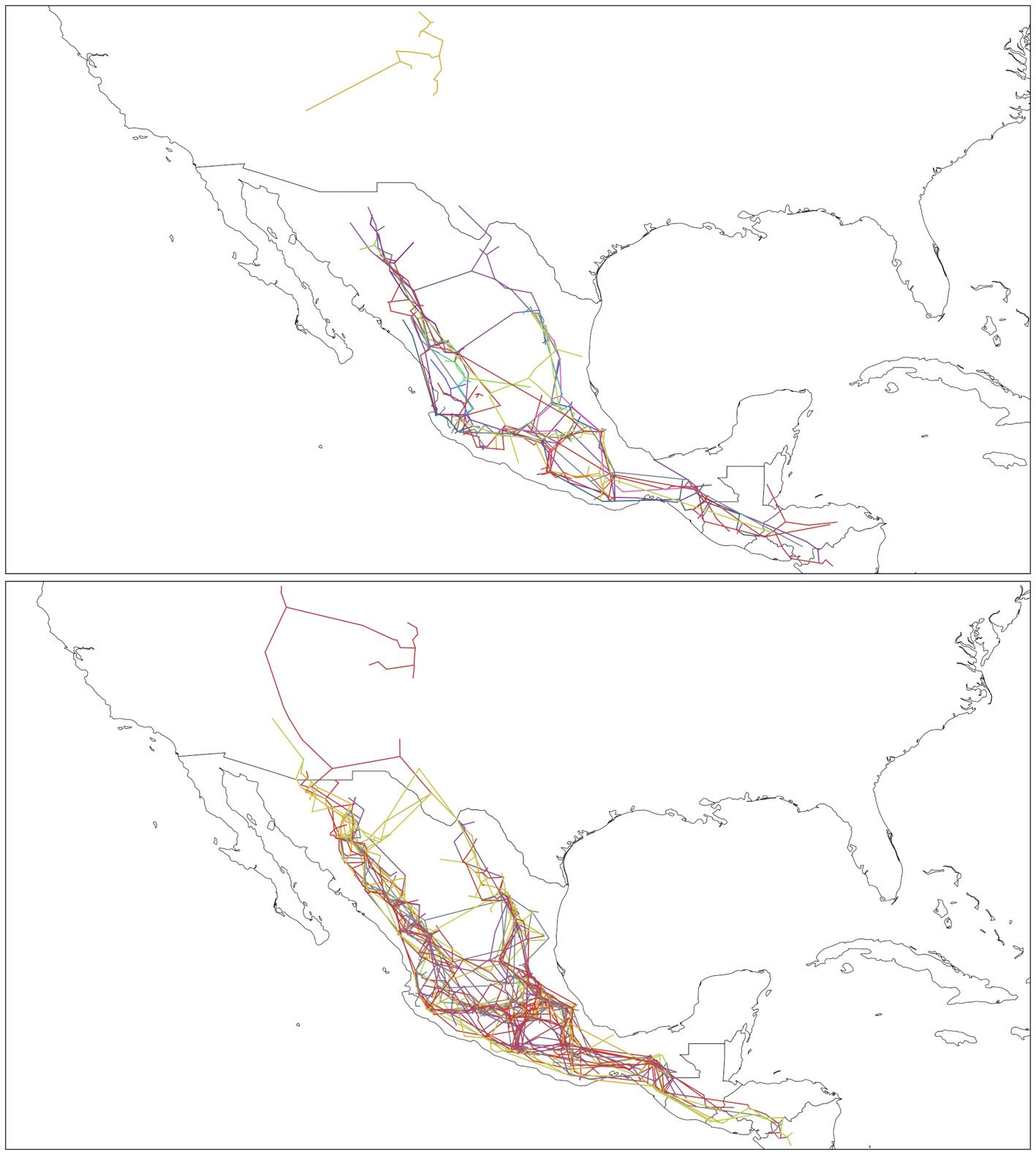
Figure 3. Individual tracks generated by Panbiotracks. Top, individual tracks from Pinus data; bottom, individual tracks from Quercus data. Maps by CF Castillo-García.
As mentioned, the algorithm for generating IGTs finds any intersection between pair of tracks to get a list of vertices from which the IGT will be built. This same algorithm is used to find the generalized nodes within IGTs. This method has various advantages, like its speed and straightforward approach. An IGT is a type of generalized track that only takes into account “true” connections, that is, intersections between individual tracks. From this point of view, it can be said that an IGT is a form of generalized track with the least ambiguity, since an overlap can be identified without any uncertainty. Considering this, a tool that can identify and generate these features is very valuable and useful.
There are, however, some pending issues regarding the IGTs and the method to identify nodes. If we consider the formal definition of a generalized track, it is necessary to add improvements to the method used and allow the program to consider other degrees of congruence between individual tracks besides the direct superposition. For example, with the current method, segments of individual tracks that are very close to each other but that do not intersect, will not be marked as part of the generalized track. This can lead to the dismissal of areas where 2 or more taxa share a similar evolutionary path, which can be represented by a generalized track, but since they do not overlap, the program does not consider their congruence. An example of this can be seen in Figure 4a, where the 2 westernmost segments are almost parallel, but the algorithm does not count them for the IGT (Fig. 6a). A potential solution is to add an option to define a buffer or area of influence around the individual tracks, and use that to compute the generalized track, but this method requires more testing to be implemented properly. There are other methods that are currently being researched for their inclusion in Panbiotracks. One is the Fréchet distance, which measures the degree of similarity between curves (Alt & Godau, 1995; Aronov et al., 2006). Another is the Hausdorff distance, which measures the distance of 2 subsets of a metric space (Bai et al., 2011; van Kreveld et al., 2022). Both concepts can potentially be used to detect and build generalized tracks with more accuracy than with present methods.
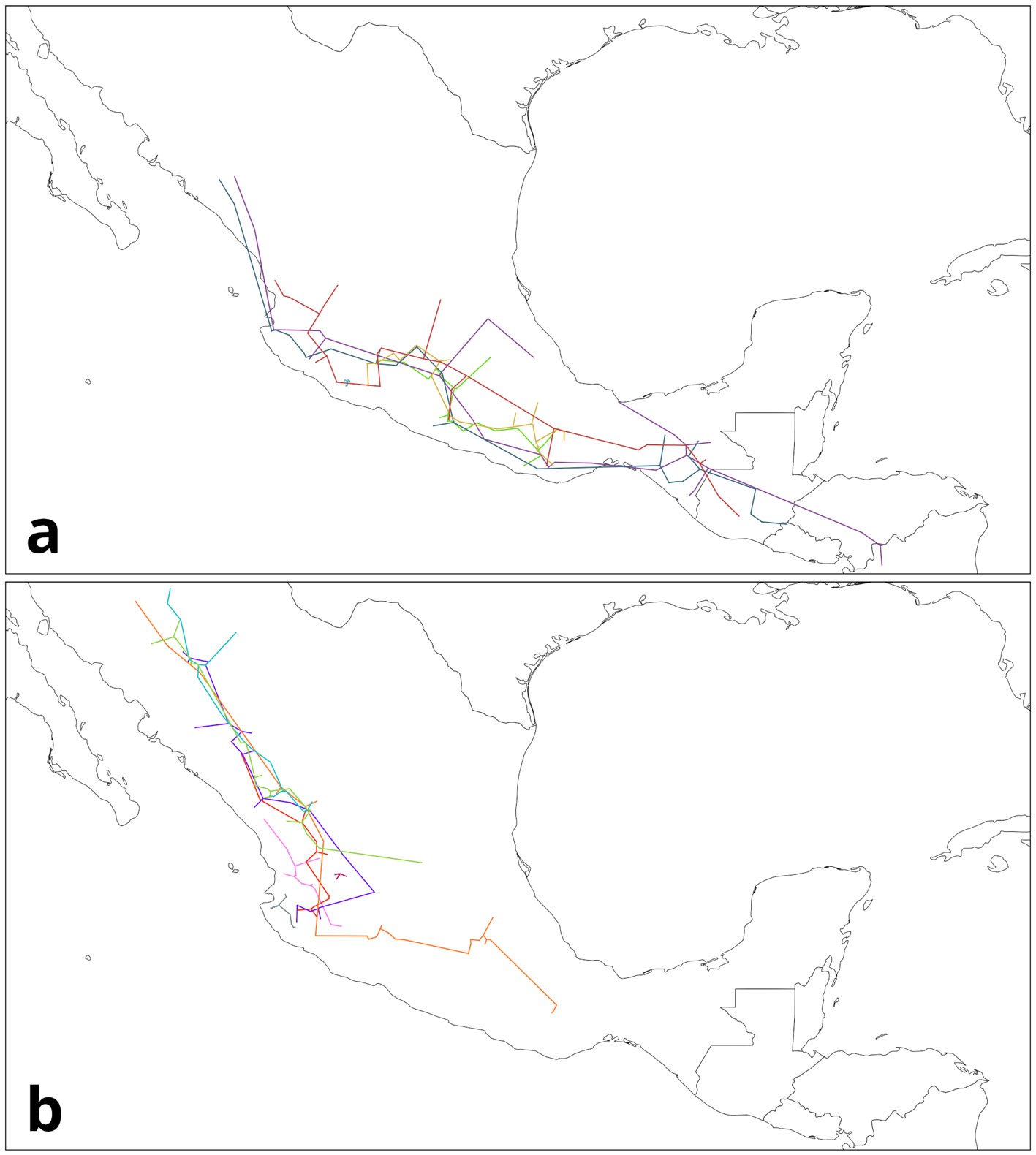
Figure 4. Groups of individual tracks from Pinus data: a) SMS group; b) SMOcc group. Maps by CF Castillo-García.
It also should be noted that Panbiotracks currently does not automatically separate the ITs that will be used for the IGTs. Because of this, it is strongly advised to first use methods like PAE-PCE (Luna-Vega et al., 1999, 2000) or NDM/NVDM (Goloboff, 2005) to segregate those ITs that are useful for building an IGT. These methods have been used to identify areas of endemism (García-Barros et al., 2002; Santiago-Alvarado et al., 2022), but they can also be used to define sets of species whose ITs are related enough to form an IGT.
The formal definition of a panbiogeographical node indicates that it is present only at the intersection of 2 or more endpoint vertices from 2 or more generalized tracks, that is, those vertices located at the periphery of the MST that only have one edge connecting them to another node (Henderson, 1989; Morrone, 2015). Since Panbiotracks takes into account all the intersections between generalized tracks, it does not quite follow this definition. However, as mentioned before, the generalized nodes can be seen as a set of which the panbiogeographical nodes are a part. As such, it is necessary to develop an improved algorithm that can filter and locate only the desired localities. This also applies for those cases where 2 terminal segments from different IGTs do not overlap. Under certain circumstances, a panbiogeographical node can be said to be present at a given location, but the IGTs might not overlap and, consequently, the software will not consider this area as a node. In Fig. 6, for example, the area towards the northwest of the map, where there are terminal ends of the IGTs, might be considered a node, but the program does not mark it. To solve this, a similar solution to that of the IGTs may be useful: define a buffer and evaluate the degree of overlap not between tracks, but between these buffers.
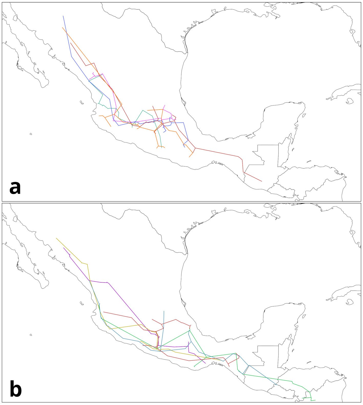
Figure 5. Groups of individual tracks from Quercus data: a) SMOcc-EVT; b) SMOcc-SMS-EVT. Maps by CF Castillo-García.
Automating track analysis and other methods in biogeography is essential and of utmost importance to the future of this field of knowledge. With the introduction of faster computer systems and programming languages specialized in data manipulation and analysis, like Python and Julia, it is necessary to develop new algorithms and improve existing ones. Moreover, another issue of great importance is to ensure that the software can be updated and improved and not let it become obsolete or dependent on outdated systems and software.
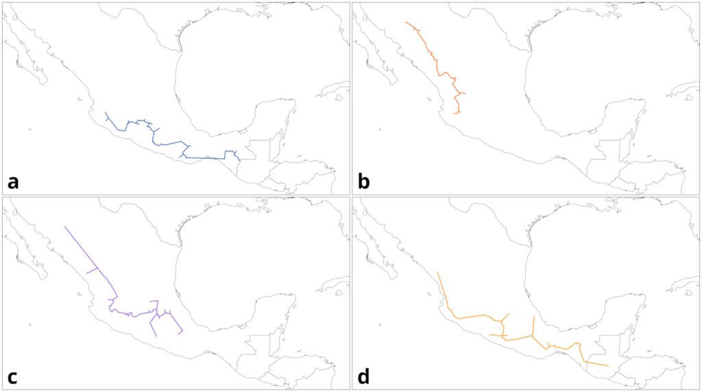
Figure 6. Generalized tracks identified from the ITs: a) IGT from the Pinus SMS group; b) IGT from the Pinus SMOcc group; c) IGT from the Quercus SMOcc-EVT group; d) IGT from the Quercus SMOcc-SMS-EVT group. Maps by CF Castillo-García.
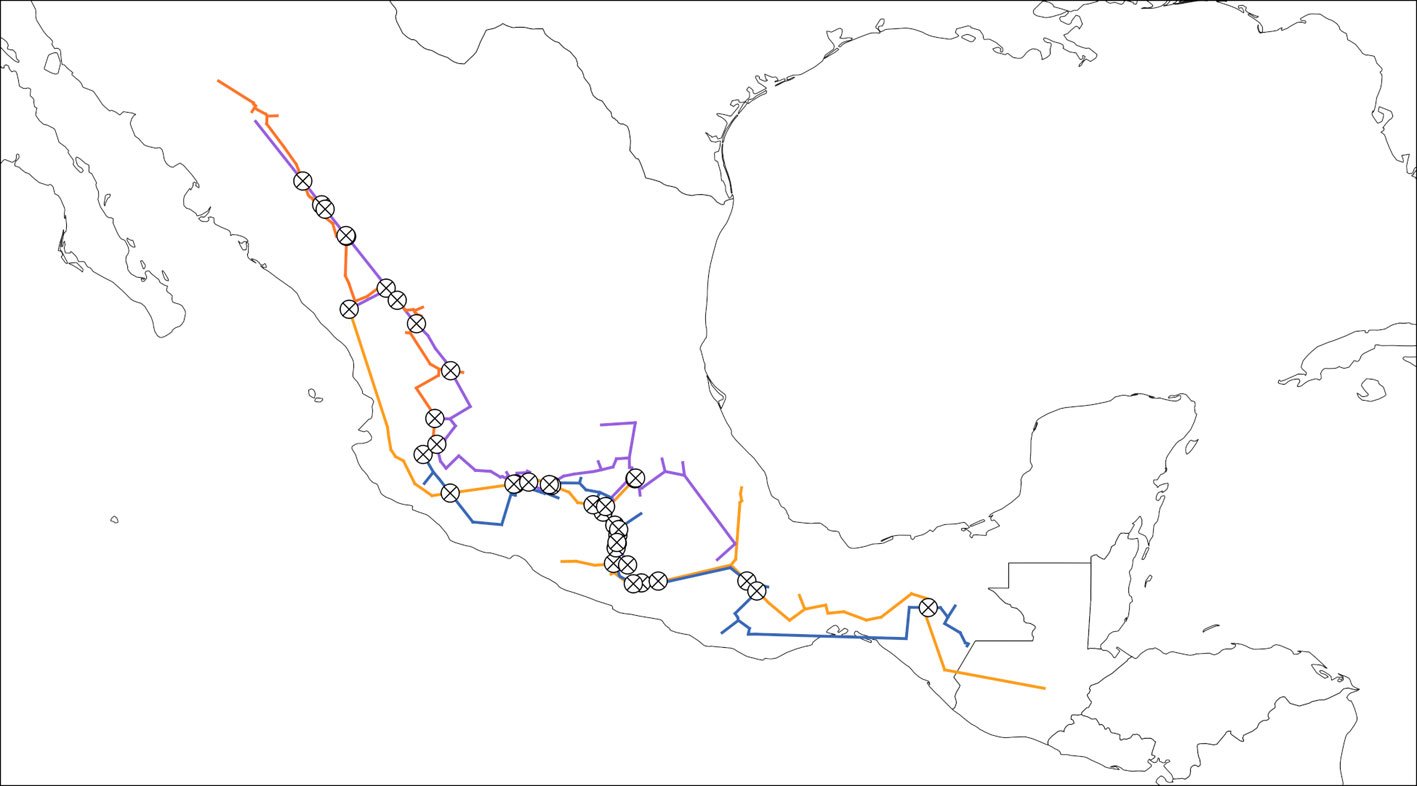
Figure 7. Generalized nodes identified from the intersections from all 4 groups. Map by CF Castillo-García.
Acknowledgments
This paper serves as a fulfillment of CFC-G for obtaining a M.Sc. degree in the Posgrado en Ciencias Biológicas, UNAM. We thank to the Secretaría de Ciencia, Humanidades, Tecnología e Innovación (Secihti) for the support of this research through a graduate scholarship (No. 1178796) to CFC-G. This work was funded by the project IN215321 (DGAPA-PAPIIT).
References
Aguilar-Estrada, L. G., & Morrone, J. J. (2022). Distributional patterns of Vetigastropoda (Mollusca) all over the world: a track analysis. Zoological Journal of the Linnean Society, 196, 442–452. https://doi.org/10.1093/zoolinnean/zlac004
Alt, H., & Godau, M. (1995). Computing the Fréchet distance between two polygonal curves. International Journal of Computational Geometry & Applications, 5, 75–91. https://doi.org/10.1142/S0218195995000064
Aronov, B., Har-Peled, S., Knauer, C., Wang, Y., & Wenk, C. (2006). Fréchet distance for curves, revisited. In Y. Azar, & T. Erlebach (Eds.), Algorithms – ESA 2006 (pp. 52–63). Springer. https://doi.org/10.1007/11841036_8
Bai, Y. B., Yong, J. H., Liu, C. Y., Liu, X. M., & Meng, Y. (2011). Polyline approach for approximating Hausdorff distance between planar free-form curves. Computer-Aided Design, 43, 687–698. https://doi.org/10.1016/j.cad.2011.02.008
Beauchamp, A. J. (1989). Panbiogeography and rails of the genus Gallirallus. New Zealand Journal of Zoology, 16, 763–772. https://doi.org/10.1080/03014223.1989.10422933
Bron, C., & Kerbosch, J. (1973). Algorithm 457: Finding all cliques of an undirected graph. Communications of the ACM, 16, 575–577. https://doi.org/10.1145/362342.362367
Brummelen, G. V. (2013). Heavenly mathematics: the forgotten art of spherical trigonometry. Princeton, NJ: Princeton University Press.
Cavalcanti, M. J. (2009). Croizat: a software package for quantitative analysis in panbiogeography. Biogeografía, 4, 4–6.
Craw, R. (1988). Continuing the synthesis between panbiogeography, phylogenetic systematics and geology as illustrated by empirical studies on the biogeography of New Zealand and the Chatham Islands. Systematic Biology, 37, 291–310. https://doi.org/10.1093/sysbio/37.3.291
Craw, R. (1989). New Zealand biogeography: a panbiogeographic approach. New Zealand Journal of Zoology, 16, 527–547. https://doi.org/10.1080/03014223.1989.10422921
Craw, R., Grehan, J., & Heads, M. (1999). Panbiogeography: tracking the history of life. Oxford, UK: Oxford University Press.
Echeverría-Londoño, S., & Miranda-Esquivel, D. R. (2011). MartiTracks: a geometrical approach for identifying geographical patterns of distribution. Plos One, 6, e18460. https://doi.org/10.1371/journal.pone.0018460
Escalante, T., Noguera-Urbano, E. A., & Corona, W. (2018). Track analysis of the Nearctic region: identifying complex areas with mammals. Journal of Zoological Systematics and Evolutionary Research, 56, 466–477. https://doi.org/
10.1111/jzs.12211
Escalante, T., Noguera-Urbano, E. A., Pimentel, B., & Aguado-Bautista, O. (2017). Methodological issues in modern track analysis. Evolutionary Biology, 44, 284–293. https://doi.org/10.1007/s11692-016-9401-8
Ferrari, A., Barão, K. R., & Simões, F. L. (2013). Quantitative panbiogeography: Was the congruence problem solved? Systematics and Biodiversity, 11, 285–302. https://doi.org/10.1080/14772000.2013.834488
Florentin, J. E., Arana, M. D., & Salas, R. M. (2016). Panbiogeographic analysis of Galianthe subgenus Ebelia (Rubiaceae). Rodriguésia, 67, 437–444. https://doi.org/10.
1590/2175-7860201667214
Gallo, V., Avilla, L. S., Pereira, R. C. L., & Absolon, B. A. (2013). Distributional patterns of herbivore megamammals during the Late Pleistocene of South America. Anais Da Academia Brasileira de Ciências, 85, 533–546. https://doi.org/10.1590/S0001-37652013000200005
García-Barros, E., Gurrea, P., Luciáñez, M. J., Cano, J. M., Munguira, M. L., Moreno, J. C. et al. (2002). Parsimony analysis of endemicity and its application to animal and plant geographical distributions in the Ibero-Balearic region (western Mediterranean). Journal of Biogeography, 29, 109–124. https://doi.org/10.1046/j.1365-2699.2002.00653.x
García-Díaz, R. F., Valdez-Hernández, E. F., Martínez-Cárdenas, L., Díaz-Nájera, F., & Ayvar-Serna, S. (2023). Diversity and distribution of Andean tubers: an agrogeographic analysis. Investigaciones y Estudios – UNA, 14, 59–70. https://doi.org/10.57201/IEUNA2313312
GBIF.org. (2016a). GBIF occurrence download. The Global Biodiversity Information Facility. https://doi.org/10.15468/DL.DGUZHT
GBIF.org. (2016b). GBIF occurrence download. The Global Biodiversity Information Facility. https://doi.org/10.15468/DL.ORDDD1
Goloboff, P. (2005). NDM/VNDM (Versión 2.5). Programs for identification of areas of endemism. Programs and documentation available at: http://www.zmuc.dk/public/phylogeny/endemism
González-Ávila, A., Contreras-Medina, R., Espinosa, D., & Luna-Vega, I. (2017). Track analysis of the order Gomphales (Fungi: Basidiomycota) in Mexico. Phytotaxa, 316, 22. https://doi.org/10.11646/phytotaxa.316.1.2
Graham, R. L., & Hell, P. (1985). On the history of the minimum spanning tree problem. Annals of the History of Computing, 7, 43–57. https://doi.org/10.1109/MAHC.1985.10011
Grehan, J. (2001). Biogeography and evolution of the Galapagos: Integration of the biological and geological evidence. Biological Journal of the Linnean Society, 74, 267–287. https://doi.org/10.1111/j.1095-8312.2001.tb01392.x
Heads, M. (2004). What is a node? Journal of Biogeography, 31, 1883–1891. https://doi.org/10.1111/j.1365-2699.2004.01201.x
Henderson, I. M. (1989). Quantitative panbiogeography: an investigation into concepts and methods. New Zealand Journal of Zoology, 16, 495–510. https://doi.org/10.1080/03014223.1989.10422918
Hernández-Cisneros, A. E., & Vélez-Juarbe, J. (2021). Palaeobiogeography of the North Pacific toothed mysticetes (Cetacea, Aetiocetidae): a key to Oligocene cetacean distributional patterns. Palaeontology, 64, 51–61. https://doi.org/10.1111/pala.12507
Kruskal, J. B. (1956). On the shortest spanning subtree of a graph and the traveling salesman problem. Proceedings of the American Mathematical Society, 7, 48–50. https://community.ams.org/journals/proc/1956-007-01/S0002-9939-1956-0078686-7/S0002-9939-1956-0078686-7.pdf
López, B., Naranjo-García, E., & Mejía, O. (2022). Diversity patterns of Mexican land and freshwater snails: a spatiotemporal approach. Revista Mexicana de Biodiversidad, 93, e933966. https://doi.org/10.22201/ib.20078706e.2022.93.3966
Luna-Vega, I., Alcántara-Ayala, O., Espinosa-Organista, D., & Morrone, J. J. (1999). Historical relationships of the Mexican cloud forests: A preliminary vicariance model applying Parsimony Analysis of Endemicity to vascular plant taxa. Journal of Biogeography, 26, 1299–1305. https://doi.org/10.1046/j.1365-2699.1999.00361.x
Luna-Vega, I., Alcántara-Ayala, O., Morrone, J. J., & Espinosa, D. (2000). Track analysis and conservation priorities in the cloud forests of Hidalgo, Mexico. Diversity and Distributions, 6, 137–143. https://doi.org/10.1046/j.1472-4642.2000.00079.x
Maya-Martínez, A., Schmitter-Soto, J. J., & Pozo, C. (2011). Panbiogeography of the Yucatán Peninsula based on Charaxinae (Lepidoptera: Nymphalidae). Florida Entomologist, 94, 527–533. https://doi.org/10.1653/024.094.0317
Miguel-Talonia, C., & Escalante, T. (2013). Los nodos: el aporte de la panbiogeografía al entendimiento de la biodiversidad. Biogeografía, 6, 30–42.
Morrone, J. J. (2014). Parsimony analysis of endemicity (PAE) revisited. Journal of Biogeography, 41, 842–854. https://
doi.org/10.1111/jbi.12251
Morrone, J. J. (2015). Track analysis beyond panbiogeography. Journal of Biogeography, 42, 413–425. https://doi.org/10.
1111/jbi.12467
Page, R. D. M. (1987). Graphs and generalized tracks: quantifying Croizat’s panbiogeography. Systematic Zoology, 36, 1. https://doi.org/10.2307/2413304
Prim, R. C. (1957). Shortest connection networks and some generalizations. The Bell System Technical Journal, 36, 1389–1401. https://doi.org/10.1002/j.1538-7305.1957.tb01515.x
Puga-Jiménez, A. L., Andrés-Hernández, A. R., Carrillo-Ruiz, H., Espinosa, D., & Rivas-Arancibia, S. P. (2013). Patrones de distribución del género Zanthoxylum L. (Rutaceae) en México. Revista Mexicana de Biodiversidad, 84, 1179–1188. https://doi.org/10.7550/rmb.32047
Rangel, T. F., Diniz-Filho, J. A. F., & Bini, L. M. (2010). SAM: A comprehensive application for Spatial Analysis in Macroecology. Ecography, 33, 46–50. https://doi.org/10.1111/j.1600-0587.2009.06299.x
Rojas-Parra, C. A. (2007). Una herramienta automatizada para realizar análisis panbiogeográficos. Biogeografía, 1, 31–33.
Rosen, B. R. (1988). From fossils to earth history: applied historical biogeography. In A. A. Myers, & P. S. Giller (Eds.), Analytical biogeography: an integrated approach to the study of animal and plant distributions (pp. 437–481). Netherlands: Springer. https://doi.org/10.1007/978-94-009-1199-4_17
Rosenberg, M. S., & Anderson, C. D. (2011). PASSaGE: Pattern Analysis, Spatial Statistics and Geographic Exegesis. Version 2. Methods in Ecology and Evolution, 2, 229–232. https://doi.org/10.1111/j.2041-210X.2010.00081.x
Santiago-Alvarado, M., Luna-Vega, I., Rivas, G., & Espinosa, D. (2022). Effect of cell size and thresholds in NDM/NVDM methods on recognizing areas of endemism. Zootaxa, 5134, 1–33. https://doi.org/10.11646/zootaxa.5134.1.1
Seberg, O. (1986). A critique of the theory and methods of panbiogeography. Systematic Zoology, 35, 369–380. https://doi.org/10.2307/2413388
Sedgewick, R., & Wayne, K. (2011). Algorithms (4th ed). Boston, Massachusetts: Addison-Wesley Professional.
van Kreveld, M., Miltzow, T., Ophelders, T., Sonke, W., & Vermeulen, J. L. (2022). Between shapes, using the Hausdorff distance. Computational Geometry, 100, 101817. https://doi.org/10.1016/j.comgeo.2021.101817
Vavrek, M. J. (2011). Fossil: palaeoecological and palaeogeographical analysis tools. Palaeontologia Electronica, 14, 16.
Vincenty, T. (1975). Direct and inverse solutions of geodesics on the ellipsoid with application of nested equations. Survey Review, 23, 88–93. https://doi.org/10.1179/sre.1975.23.176.88
Waters, J. M., Trewick, S. A., Paterson, A. M., Spencer, H. G., Kennedy, M., Craw, D. et al. (2013). Biogeography off the tracks. Systematic Biology, 62, 494–498. https://doi.org/10.1093/sysbio/syt013
Wormald, N. C. (1984). Generating random regular graphs. Journal of Algorithms, 5, 247–280. https://doi.org/10.1016/
0196-6774(84)90030-0
Zunino, M., & Zullini, A. (2003). Biogeografía: la dimensión espacial de la evolución (Vol. 259). Ciudad de México: Fondo de Cultura Económica.


