Wild chia (Salvia hispanica) populations, endangered under global warming scenarios
Peligro de extinción de poblaciones silvestres de chía (Salvia hispanica) bajo escenarios de calentamiento global
Sabina Lara-Cabrera a, *, Gleisery Rivas-Jaimes a, David A. Prieto-Torres b, c, Cuauhtémoc Sáenz-Romero c, d, Lourdes Núñez-Landa a, Guillermo Orozco-de Rosas e, Juan-Carlos Montero-Castro a
a Universidad Michoacana de San Nicolás de Hidalgo, Facultad de Biología, Laboratorio de Biodiversidad y Biogeografía de Plantas, Gral. Francisco J. Múgica s/n, Ciudad Universitaria, Edificio B2, 3er piso, Felicitas de Río, 58030 Morelia, Michoacán, Mexico
b Universidad Nacional Autónoma de México, Facultad de Estudios Superiores Iztacala, Laboratorio de Biodiversidad y Cambio Climático, Av. de los Barrios 1, Los Reyes Iztacala, 54090 Tlalnepantla, Estado de México, Mexico
c Laboratorio Nacional de Biología del Cambio Climático, SECIHTI, Mexico
d Universidad Michoacana de San Nicolás de Hidalgo, Instituto de Investigaciones sobre los Recursos Naturales, Av. Juanito Itzícuaro s/n, Col. Nueva Esperanza, 58337 Morelia, Michoacán, Mexico
e Chia Blanca, S.C. de R.L., La Paz No. 54, 45470 Acatic, Jalisco, Mexico
*Corresponding author: sabina.lara@umich.mx (S. Lara-Cabrera)
Received: 25 July 2025; accepted: 14 January 2026
Abstract
The conservation of crop wild relatives is particularly worrisome under global warming scenarios given their potential as sources of diversity for cultivars. Here we evaluate the potential effect of climate change through ecological niche modeling for wild chia (Salvia hispanica) populations as the closest crop wild relative. Current and future (2040, 2060, 2080) climatic conditions were modeled using 4 global climate models (ACCESS-CM2, BCC-CSM2-MR, MIROC6, and CanESM5) and 2 shared socioeconomic pathways (SSP2-4.5 and SSP5-8.5), accounting for both limited and long-distance dispersal scenarios. Current potential wild S. hispanica distribution is 192,789 km², 16.72% in climatically stable areas and coinciding with 184 Nature Conservancy Areas in Mexico and Guatemala. Unfortunately, by 2040, 2060, and 2080 wild chia’s potential distribution would reduce by 60.81 to 83.07%, respectively under optimistic scenarios with potential of dispersion as well as pessimistic and nondispersal scenarios. Furthermore, the most sensitive areas are in the Trans-Mexican Volcanic Belt, Pacific Coast, and Guatemala, which also are reportedly the most genetically diverse populations. We urge conservation efforts to increase wild germplasm collections and embark on in situ conservation with local communities to preserve the genetic reservoir of the species for future crop breeding.
Keywords: Climate change; Environmental suitability; Species distribution; Vulnerability risk
Resumen
Una de las mayores preocupaciones ante escenarios de cambio climático es la conservación de parientes silvestres de cultivos, dado su potencial como fuente de diversidad genética. Aquí evaluamos el efecto potencial del cambio climático actual y futuro (2040, 2060, 2080) para poblaciones silvestres de chía (Salvia hispanica), el pariente silvestre más cercano, a través de modelación del nicho ecológico utilizando 4 modelos de cambio climático (ACCESS-CM2, BCC-CSM2-MR, MIROC6 y CanESM5) bajo 2 trayectorias socioeconómicas (SSP2-4.5 y SSP58.5), considerando también dispersión limitada y de larga distancia. La distribución potencial actual de poblaciones silvestres de S. hispanica es de 192,789 km² y 16.72% en áreas climáticamente estables que coinciden con 184 áreas naturales de conservación de México y Guatemala. Desafortunadamente hacia 2040, 2060 y 2080 su distribución se reducirá de -60.81% a -83.70% respectivamente bajo trayectoria socioeconómica optimista con dispersión a larga distancia y pesimista con dispersión limitada. Adicionalmente las regiones más sensibles coinciden con las que se han reportado como genéticamente diversas en el Cinturón Volcánico Trans-Mexicano, Costa del Pacífico y Guatemala. Llamamos a incrementar los esfuerzos de conservación, aumentar las colecciones de germoplasma e iniciar proyectos de conservación in situ comunitarios con miras a conservar el reservorio genético del cultivo.
Palabras clave: Cambio climático; Idoneidad ambiental; Distribución de especies; Riesgo por vulnerabilidad
Introduction
Chia is a native crop of Mesoamerica (Cahill, 2003; Kirchhoff, 2000). Several attributes related to the high omega-3 content of chia (Salvia hispanica L.) have led to its steadily growing global consumption (Ali et al., 2012; Grancieri et al., 2019; Katunzi-Kilewela et al., 2021). While current estimates of global production increased in Paraguay, Bolivia, and Mexico from ca. 13,000,000 in 2019 to 18,000,000 in 2023 (Anuario Estadístico de Producción Agrícola, 2025) and consumption was estimated at 80,000 to 100,000 tons per year (Góral, 2025), little attention has been given to the distribution and conservation of wild chia populations, which are considered a Crop Wild Relative (CWR) and thus an important source of genetic variability for the crop (Maxted et al., 2006). The earliest documentary records, including the “Matrícula de tributos” (2022) and the “Relaciones geográficas de la Nueva España” (Murrieta-Flores et al., 2020), highlight the significance of chia in pre-Hispanic diets, ranking third in importance after maize and beans. However, the timeline of its domestication remains uncertain. The only unequivocal archaeobotanical evidence is nutlets dated to 1,750 years before present. Some studies suggest an earlier domestication event around 4,500 years ago based on pollen records (Sosa et al., 2016), although these may only be assignable to the genus Salvia rather than specifically to S. hispanica (LaraCabrera et al., 2025). Therefore, major questions regarding the identity and timeline of chia’s domestication cannot yet be addressed. Available evidence strongly suggests that domestication occurred in Mexico-Guatemala (i.e., Mesoamerica), a recognized center of origin for many globally important crops (Colunga-García Marín & Zizumbo-Villareal, 2004; Flannery, 1973). Chia has been included in Mexico’s inventory of 310 priority CWR species (Contreras-Toledo et al., 2018) and the global CWR inventory proposed by Harlan and De Wet (Vincent et al., 2013). The closest chia relatives are wild chia populations, making their study and conservation a pressing need. The conservation of CWRs is a global concern, as emphasized by the FAO, which recognizes their critical role in ensuring future food security in the context of global change (Kaeslin et al., 2012). In this context, the first step toward developing effective conservation strategies, as highlighted by Goettsch et al. (2021), is to generate accurate distribution maps, beginning by data curation to remove misidentified records and cultivated specimens. Here we apply ecological niche modeling using Maxent to wild chia populations in order to: 1) approximate the species’ Grinnellian niches (Peterson et al., 2011; Rödder & Engler, 2011); and 2) project future distribution under global warming scenarios (Dormann et al., 2007). Previous work by Durán et al. (2016) modeled environmental suitability for the periods 2041-2060 and 2061-2080, also using herbarium specimens. However, it remains unclear whether they distinguished wild from cultivated specimens, a key factor, as a mixed dataset could affect model accuracy due to differences in abiotic tolerance and dispersal capability. Here we carefully selected only wild chia specimens based on morphological traits, avoiding individuals exhibiting a domestication syndrome. For example, in wild populations, the fruiting calyx remains open, allowing nutlet release whereas in cultivated chia nutlets remain enclosed in the fruiting calyx. Chia nutlets (often misinterpreted as seeds) produce mucilage upon contact with water, and as has been described for thyme, the hydrated mericarp swells and pushes the calyx open to expose the nutlet (Bouman & Meeuse, 1992). Domesticated plants also tend to have larger overall size, inflorescences, and flowers (Cahill, 2003, 2005). Our dataset was subsequently used to model future niche distributions for the years 2040, 2060, and 2080 under optimistic and pessimistic Shared Socioeconomic Pathways (SSPs) following the Intergovernmental Panel on Climate Change (IPCC, 2022), global warming being one of the most severe threats to CWR conservation. We also considered chia’s potential for dispersal and colonization of new areas. Chia likely has limited natural dispersal via water (hydrochory or ombrochory; Zona, 2017), and when calices remain open gravity plays a role as nutlets fall near the parent plant and germinate nearby (phylomatri sensu Cheplick, 2021). Yet long-distance dispersal, potentially through human activity, may become crucial under accelerated climate change. Finally, given the serious conservation threat for many CWRs through land-use change (Goettsch et al., 2021), we evaluated the spatial overlap between the modeled distributions and the Mexican and Guatemalan Natural Conservation Areas. These areas represent an immediate opportunity for passive CWR conservation, especially at biodiversity hotspots where indigenous communities have managed the surrounding species for millennia resulting through domestication in a mosaic of landraces (Vincent et al., 2022). Our results offer valuable guidance for policymakers and plant breeders, enabling the identification of wild chia populations for in situ conservation and seed bank enhancement for ex situ conservation. Early, informed decisions are essential for preserving the genetic diversity of this culturally and nutritionally important crop.
Materials and methods
Biological data acquisition. Occurrence data follow Lara-Cabrera et al. (2025) identifying wild specimens from digitized herbarium collections at the Consortium of California Herbaria ([https://cch2.org/portal/collections/] RSA, UCR) MEXU (https://datosabiertos.unam.mx/ biodiversidad/), Portal Torch Herbaria ([https://portal. torcherbaria.org/portal/index.php] ASU, CIIDIR, COLO, DES, IBUG, IND, MICH, UNM, UTEP, WIS), US (https:// collections.nmnh.si.edu/search/botany/), and herbarium review (IEB). Domestication status was determined based on botanical descriptions (Klitgaard, 2012; Ramamoorthy, 1996; Wood & Harley, 1989) and cross-checked with studies on domestication syndrome traits in the species (Cahill, 2003, 2005; Calderón-Ruíz et al., 2021). Overall, wild specimens are recognized as shorter plants (30-100 cm tall), with short inflorescences (up to 10 cm), bearing 3 to 6 flowers per verticillaster, corolla tube 8-9 mm long that is almost entirely enclosed by the calix, and smaller fruiting calyces remaining open at maturity. Note that the ability to maintain open calyces to release the nutlets is a key trait distinguishing most domesticated varieties, as in the latter the calyx remains closed. All records were carefully reviewed to eliminate ambiguities such as duplicates, points located on roads or residential areas, and records with a spatial separation of less than 2 km to reduce spatial autocorrelation (Boria et al., 2014; Legendre, 1993; Peterson et al., 2011). Following Prieto-Torres et al. (2020, 2021) and PrietoTorres (2024), recent records (2001-2022) were subjected to an environmental outlier exclusion procedure. Records were removed if their values for Worldclim bioclimatic variables Bio 1 (annual mean temperature), Bio 5 (maximum temperature warmest month), Bio 12 (annual precipitation), and Bio 15 (precipitation seasonality) fell outside the upper or lower quartiles of the same variables calculated from herbarium records dated between 19702000. Those variables were used because other studies (e.g., Núñez-Landa et al., 2023; Prieto-Torres et al., 2020, 2021) have found them useful in the data depuration process. The final occurrence dataset included 55 independent localities of species presence, corresponding to the full list published by Lara-Cabrera et al. (2025). Environmental information for current and future scenarios. Available climatic layers were downloaded from Worldclim 2.1 (Fick & Hijmans, 2017; Hijmans et al., 2005) at a spatial resolution of 30 arc-seconds (~ 1 km²). These bioclimatic variables, derived from monthly temperature and precipitation data, reflect longterm climatic trends. Nonetheless, variables Bio 8 (mean temperature wettest quarter), Bio 9 (mean temperature dries quarter), Bio 18 (precipitation of wettest quarter), and Bio 19 (precipitation of coldest quarter) were excluded due to potential spatial artifacts in their interpolated surfaces, which could negatively affect model performance (Booth, 2022; Escobar et al., 2014). Checking for such anomalies is particularly important when modeling across broad regions, as in this study, to prevent localized irregularities which could bias overall results (Booth, 2022). And although soil properties influence species distributions by affecting plant physiology, growth, and survival (Eamus et al., 2013; Velazco et al., 2017), we focused exclusively on climatic variables because no reliable projections of edaphic variables exist for future scenarios (Tomlinson et al., 2020). Moreover, temperature and precipitation strongly influence soil properties, so climatic variables are expected to indirectly capture part of the soil-related variability. This reasoning is consistent with studies highlighting climate as the main driver for long-term distributional shifts (Dantas et al., 2020; Hartmann et al., 2022). To avoid model overfitting due to collinearity among variables (Dormann et al., 2013), we employed a twostep process to select relevant predictors and reduce dimensionality (Cobos et al., 2019). First, Spearman and Pearson correlation coefficients were used to exclude variables with correlations greater than 0.8 and with a variance inflation value greater than 4 (Díaz-Vallejo et al., 2024; Dupin & Smith, 2019). Both coefficients were used because normality tests indicated that each variable could exhibit different spatial patterns, and a single test would not be feasible due to high spatial autocorrelation among variables, thereby justifying the combined use of both correlation measures (Díaz-Vallejo et al., 2024). Second, a principal component analysis (PCA, Janeković & Novak, 2012) was performed on the original 15 climatic variables across the study area to retain those that collectively explained at least 95% of the total variance (Hanspach et al., 2011). These procedures were performed in R using libraries “corplot”; “usdm” (Wei & Simko, 2017), and “ENMGadgets” (Barve & Barve, 2016). The best climatic data approach was selected based on statistical performance evaluated with the “kuenm” R package (Cobos et al., 2019). For future climate projections, we considered 2 Shared Socioeconomic Pathways from the Coupled Model Intercomparison Project (CMIP6): SSP2-4.5, representing a middle-of-the-road scenario with moderate emissions; and SSP5-8.5, a high-emission scenario reflecting continued fossil fuel dependence and rapid economic growth (Riahi et al., 2017). Projections were generated for 3 future timeframes: 2041–2060 (hereafter 2040), 2061– 2080 (hereafter 2060), and 2070-2090 (hereafter 2080), using 4 General Circulation Models: ACCESS-CM2, BCCCSM2-MR, MIROC6, and CanESM5. These models were selected based on their ability to simulate ENSO dynamics and associated interannual variability in precipitation and temperature (Bi et al., 2013; Watanabe et al., 2010; Zelinka et al., 2020), which are key drivers of climate patterns within the range of S. hispanica and and the whole biota of Central American and Mexico. Therefore, this selection ensures that the models capture climate processes directly relevant to the species’ environmental niche and potential distribution (Jin et al., 2025). The environmental variables selected were cropped to a region defined as M used for model calibration processes (Barve et al., 2011; Soberón & Peterson, 2005). The vectorial polygon defining M was constructed by intersecting species occurrence records with maps of terrestrial ecoregions (Dinerstein et al., 2017) and Neotropical Biogeographic provinces (Morrone et al., 2017). Although several valid approaches exist to define the M area in ecological niche modeling, we selected this method because it is not only straightforward but also highly operational (Rojas-Soto et al., 2024). Ecological niche and potential species distribution. Species models were performed with Maxent 3.4.3 (Phillips et al., 2006) and the R package “kuenm” (Cobos et al., 2019). Maxent constructs the most probable species distribution based on presence-only data and environmental variables through machine learning algorithms, as it is recognized as one of the most effective tools in terms of predictive performance (Elith et al., 2006). The “kuenm” R package was used to generate multiple candidate models by combining different sets of environmental variables (non-correlated and PCAreduced) with a range of Maxent calibration parameters (described below) to select the optimal model and subsequently project it to climate scenarios for 2040, 2060, and 2080. Occurrence records were initially split into 2 datasets: 80% were randomly selected for model training, while the remaining 20% were used for internal validation of the final model. During the calibration step, we created spatial folds using 80% of the records for training, and spatial cross-validation was applied. This approach allowed us to test 992 candidate models resulting from all 62 combinations of Maxent feature classes and 8 regularization multipliers (0.2, 0.4, 0.5, 1, 2, 6, 8, 10) and the 2 sets of variables (non-correlated and PCA-derived), in order to select the optimal set for the final modeling (Cobos et al., 2019). Optimal models were selected based on 3 criteria: statistical significance via partial ROC partial test (Peterson et al., 2008), Akaike’s information criterion for small sample sizes (AICc; Akaike, 1974), and an omission rate below 5% (Anderson et al., 2003). Final models were generated using 1,000 iterations and 10 replicates. Next, the models were projected onto future climate scenarios using 3 extrapolation settings: no extrapolation or clamping, extrapolation without clamping, and both extrapolation and clamping. These approaches are essential to identify novel climatic conditions under future scenarios, potentially suitable for the species based on extreme values of ecological variables (Elith et al., 2011; Peterson et al., 2018; Stohlgren et al., 2001). In this context, to detect future regions with non-analogous climatic conditions relative to the present, we implemented the MOP (Mobility-Oriented Parity) test (Owens et al., 2013). This test identifies zones that represent strict extrapolations of the model, which are associated with higher uncertainty and should be interpreted with caution (Alkishe et al., 2017). The Maxent outputs in “cloglog” format were converted to binary presence-absence maps using a threshold equal to the 10th percentile of training presence. This threshold minimizes commission errors by excluding only the lowest 10% of suitability scores, thus retaining predictions considered at least as suitable as the occurrence records (Liu et al., 2013). The binary maps for each Shared Socioeconomic Pathway (SSP2-4.5 and SSP5-8.5) and time period (2040, 2060, and 2080) were generated by overlaying the outputs from 4 selected Atmosphere-Ocean General Circulation Models (ACCES-CM2, BCC-CSM2MR, MIROC6, and CanESM5). Herein, a grid cell was classified as “presence” if at least 3 of the 4 models agreed on the presence prediction for that cell (e.g., Nuñez-Landa et al., 2023; Gama-Rodríguez et al., 2024). Spatial analyses and general metrics. The current binary map was compared with each future projection by overlaying and summing them, to define climatically stable areas, where a cell was considered “climatically stable” if the species’ environmental conditions were predicted therein for all evaluated periods (Collevatti et al., 2013). It is important to note that this does not imply that the local climate remains unchanged, but rather that the cell stays within the species’ tolerable range, allowing potential persistence (Terribile et al., 2012). Identifying such areas is important because they often harbor higher intraspecific genetic diversity (Hewitt, 2004). Besides, a range gain was defined when the number of pixels predicted to be suitable for distribution areas in the future were greater than those estimated in the present, and the opposite case was interpreted as range contraction for the species. Given that a species’ dispersal capacity can influence its ability to colonize new areas (Marco et al., 2011), we conducted this evaluation under 2 contrasting dispersal scenarios: short-distance dispersal (SDD), where suitable future areas were limited to those overlapping with the current distribution, and long-distance dispersal (LDD), where suitable areas projected for the future but not currently occupied were also considered. In both cases, geographic barriers defined by the M area were assumed to limit species dispersal, and ecological interactions between species were omitted (Atauchi et al., 2020; Peterson et al., 2002). For projections predicting a loss of suitable areas, we calculated the differences (current vs. future) in values of the bioclimatic and elevation variables to identify the environmental changes associated with this loss (Cobos & Bosch, 2018; Atauchi et al., 2020). The geographic centroid of the binary maps (for each present and future projections) was computed using the coordinates of all presence-value cells, with the constraint that the centroid must lay within the presence area. To enhance discussion, centroid shift was estimated in all scenarios and temporalities and actual km² and displacement direction estimated in R through the haversine formula proposed by Inman (1835). Additionally, the mean elevation and its range for each temporality were extracted by coupling future climate projection pixels with a digital elevation model. Both analyses were performed with the “terra” R package (Hijmans, 2025) Finally, we assessed the overlap between the current and projected species distribution and Natural Protected Areas (NPAs) in Mexico (https://www.gob. mx/conanp#1692) and Guatemala (https://conap.gob.gt/ listado-de-areas-protegidas/; IUCN & UNEP-WCMC, 2025). This was done by intersecting current and future binary distribution maps with the raster layers of official NPAs to identify key regions where in situ conservation of chia may be crucial in the face of land use change, contributing to risk mitigation through habitat protection.
Results
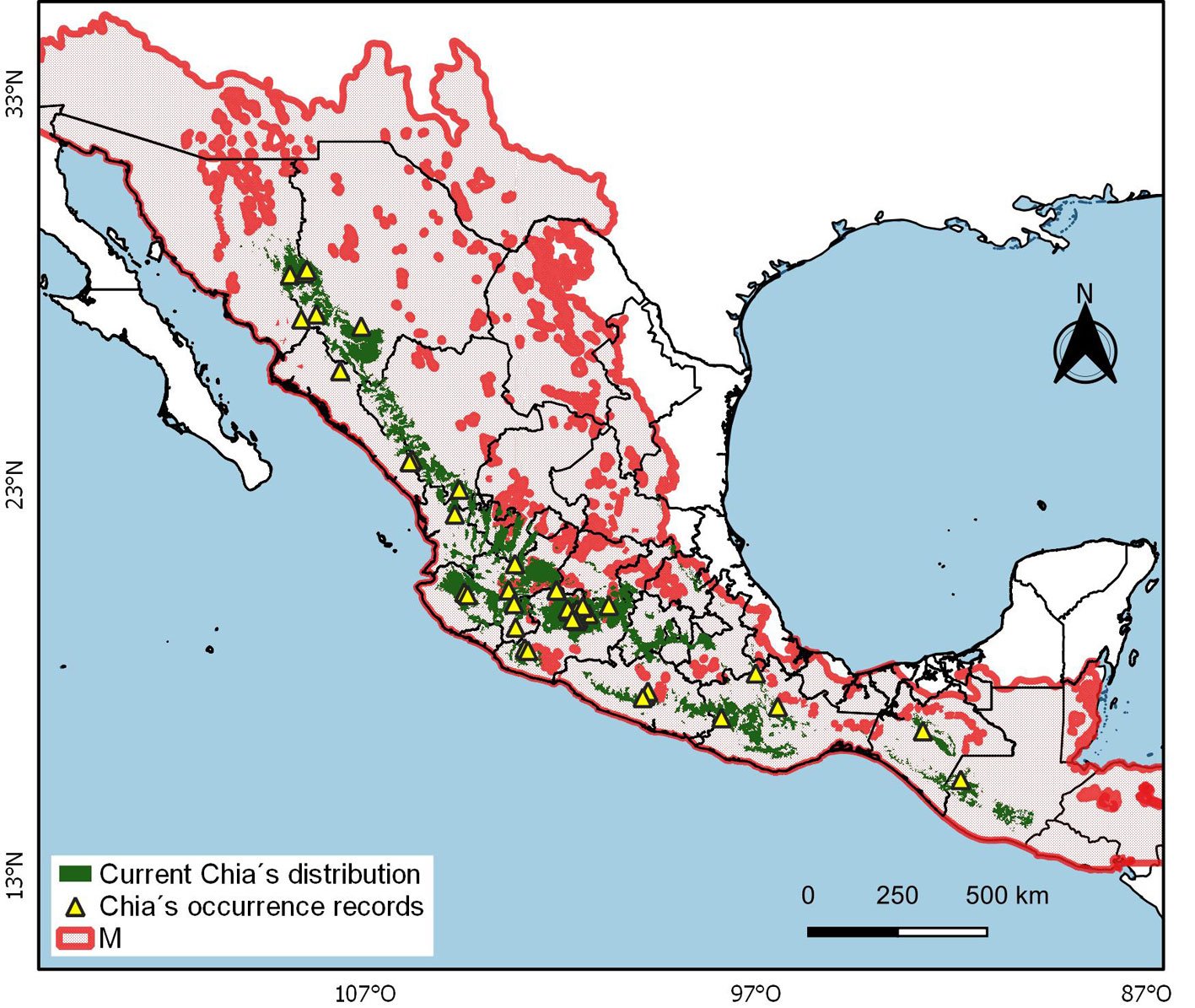
Current distribution pattern. The potential distribution model for S. hispanica was adequately calibrated, as indicated by the mean AUC ratio (1.85), minimum AIC value (708.46), statistically significant partial ROC test (0.00), and 0 omission error. The default plot produced shows both omission rates and AICc values for all tested models (Supplementary material: Fig. 1). The final model used a regularization multiplier of 2 and included the feature classes quadratic, product, and hinge. The most important variables that define the first principal component (PC1) are Bio1, Bio3, Bio6, Bio11, and Bio12, whereas the second component (PC2) is primarily defined by Bio12, Bio14, Bio15, and Bio17. The estimated current potential distribution area for wild chia is 192,789 km², primarily located across the biogeographic regions of the Sierra Madre Occidental, Trans-Mexican Volcanic Belt, Sierra Madre del Sur, and Sierra Madre de Chiapas, extending into Guatemala (Fig. 1). In Mexico, chia is distributed from the northeastern states (Sonora, Chihuahua, Durango, and Sinaloa), through the western and central regions, and into the southeast (Guerrero, Oaxaca, and Chiapas). To assess average population shift regarding latitude and longitude we estimated the centroid at 21.0367 oN, -102.231 oW (Jalisco Altos Sur, NW Jalisco, Mexico), average elevation 1,971.1 m and elevational range 1708.6 – 2211.3 m (Table 1). A valuable finding is that 11.51% (i.e., 22,206 km²) of the current projected distribution lies within NPAs. In Mexico the current potential distribution overlaps with
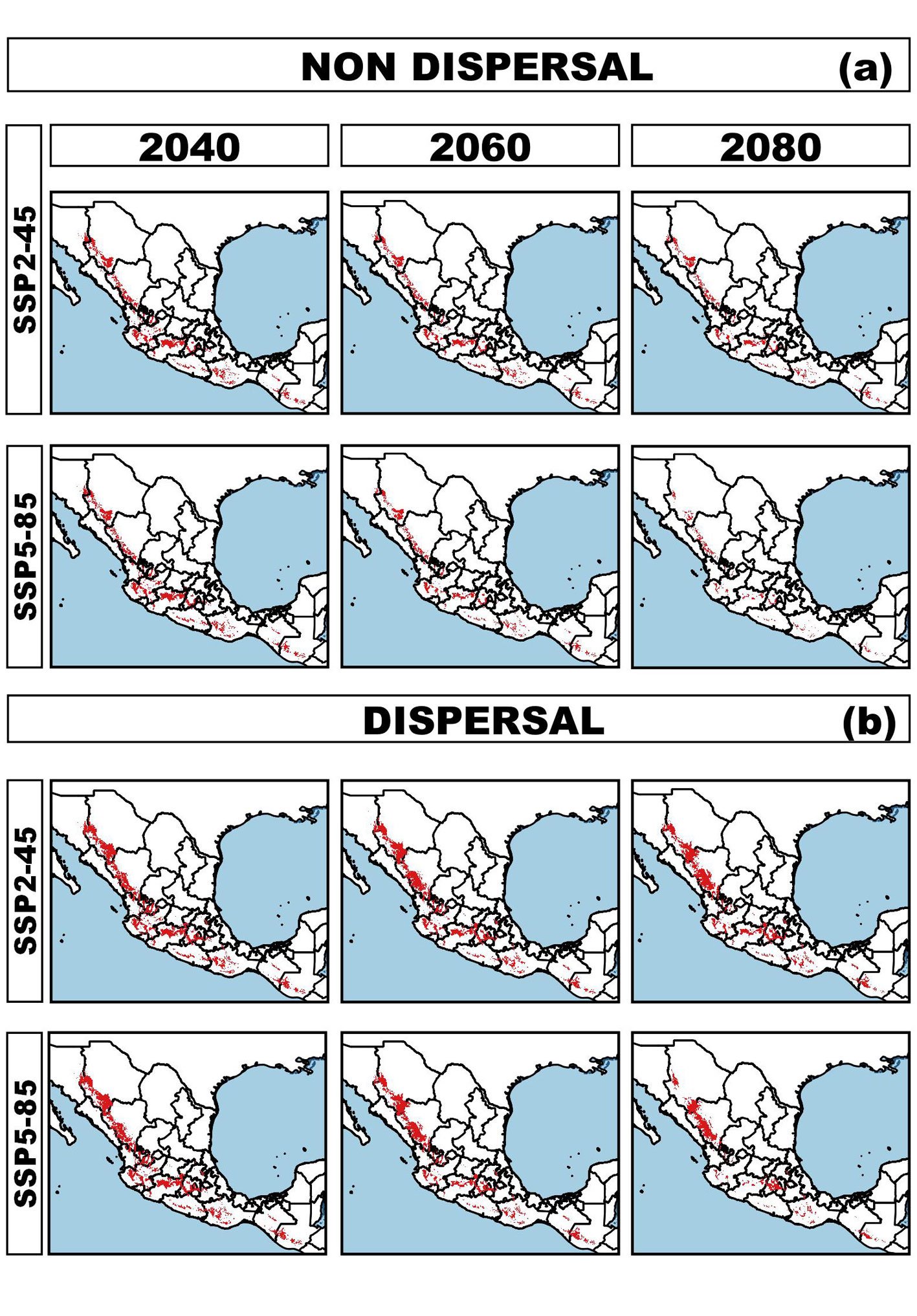
135 NPAs, including 9 Biosphere Reserves (UNESCOMAB), Flora and Fauna Protected Areas, Protected Areas for Natural Resources, National, State, Municipal Parks, and Voluntary Conservation Areas. Whereas in Guatemala the current potential distribution overlaps with 49 areas, including one Biosphere Reserve (UNESCOMAB), Natural Reserves, National and Regional Parks, Definitive Veda Zones, Forest Reserves and Use Reserves (Supplementary material: Table 1). Projected distribution patterns under non-dispersal and dispersal scenarios. The potential distribution of wild S. hispanica populations for 2040, 2060, and 2080, modeled considering non dispersal (i.e., SDD), highlights a concerning and pessimistic trend of habitat loss (Table 1, Fig. 2a). Under the optimistic global warming SSP24.5 scenario, the potential distribution area is projected to lose 38.27% by 2040, 50.07% by 2060 and 60.81% by 2080, leaving only a remaining area of 119,002 km², 96,250 km², and 75,551 km², respectively. In contrast, under the pessimistic warming scenario (SPS5-8.5), the remaining area is expected to be 32,638 km², reflecting a dramatic 83.07% loss of the current distribution. The loss of suitable habitat also extends to populations currently located within NPA: by 2040 only 15,879 km² (i.e., 13.34% of remaining suitability areas) would be within NPA and by 2080 these values are projected to decline further to 11,502 km² (i.e., 15.22%) under the optimistic scenario, and 6,195 km² (18.98%) under the pessimistic one. Furthermore, the geographic centroid of the species’ distribution is expected to shift in both longitude and latitude, accompanied by notable elevational shifts. In the SSP2-4.5 scenario, the mean elevation (currently 1,971.1 m) is projected to increase to 2,246.4 m (range: 2,0572,420.1 m), and to 2,376 m (range: 2,194-2,542.1 m) under SSP5-8.5. This corresponds to an average upward shift in elevation of 275.3 m and 405 m, respectively, along with a contraction of the current elevational range from 503 m to 357 m and 348 m under each scenario. Conversely, under the dispersal scenario (i.e., LDD), the projected future distributions are less alarming, although still indicative of significant habitat changes. These models assume the species eventually could colonize newly suitable areas, although likely requiring human-assisted dispersal. Projected distributions under
| Models | Potential distribution (pixels / km²) | Within NPA — Pixels (%) | % present vs. future | Change proportion attributable to GCC | Centroid displacement (km) and direction | Average elevation (m) | Min. elevation (m) | Max. elevation (m) |
|---|---|---|---|---|---|---|---|---|
| Current | 192,789 | 22,206 (11.51) | – | – | 21.0367, -102.231 | 1,971.1 | 1,708.6 | 2,211.3 |
| 2040 SSP2-4.5 | 119,002 | 15,879 (13.34) | 8.24 | -38.27 | 76.51 towards NW | 2,126.7 | 1,912.6 | 2,324.5 |
| 2060 SSP2-4.5 | 96,250 | 13,701 (14.23) | 7.1 | -50.07 | 81.13 towards NW | 2,184.9 | 1,984.1 | 2,372.2 |
| 2080 SSP2-4.5 | 75,551 | 11,502 (15.22) | 5.9 | -60.81 | 89.8 towards N-NW | 2,246.4 | 2,057 | 2,420.1 |
| 2040 SSP5-8.5 | 117,304 | 15,622 (13.32) | 8.1 | -39.15 | 14.71 towards SW | 2,130.4 | 1,915.5 | 2,329.6 |
| 2060 SSP5-8.5 | 77,794 | 12,060 (15.50) | 6.3 | -59.65 | 90.63 towards N-NW | 2,233 | 2,035.2 | 2,413.6 |
| 2080 SSP5-8.5 | 32,638 | 6,195 (18.98) | 3.2 | -83.07 | 84.18 towards N-NW | 2,376 | 2,194 | 2,542.1 |
| Models | Potential distribution (pixels / km²) | Within NPA — pixels (%) | % present vs. future | Change proportion attributable to GCC | New area — pixels / km² | New area — % | Centroid displacement (km) and direction | Average elevation (m) | Min. elevation (m) | Max. elevation (m) |
|---|---|---|---|---|---|---|---|---|---|---|
| Current | 192,789 | 22,206 (11.51) | – | – | – | – | 21.0367, -102.231 | 1,971.1 | 1,708.6 | 2,211.3 |
| 2040 SSP2-4.5 | 145,180 | 19,217 (13.24) | 9.96 | -24.69 | 26,178 | 18.03 | 114.4 towards NNW | 2,182.8 | 1,960.6 | 2,390.6 |
| 2060 SSP2-4.5 | 137,076 | 19,513 (14.24) | 10.12 | -28.90 | 40,826 | 29.78 | 140.85 towards NW | 2,277.5 | 2,065 | 2,475.4 |
| 2080 SSP2-4.5 | 125,364 | 18,474 (14.74) | 9.58 | -34.97 | 49,813 | 39.73 | 151.64 towards NW | 2,365.1 | 2,173.8 | 2,542.3 |
| 2040 SSP5-8.5 | 149,217 | 19,778 (13.25) | 10.25 | -22.60 | 31,913 | 21.39 | 117.54 towards NNW | 2,197.8 | 1,972.1 | 2,409.6 |
| 2060 SSP5-8.5 | 123,825 | 18,499 (14.94) | 9.59 | -35.77 | 46,031 | 37.17 | 127.45 towards NNW | 2,341.8 | 2,141 | 2,527.1 |
| 2080 SSP5-8.5 | 78,662 | 14,117 (17.95) | 7.3 | -59.20 | 46,024 | 37.17 | 202.01 towards NW | 2,508.4 | 2,346.2 | 2,655.3 |
Projected distributions under both SSP2-4.5 and SSP5-8.5 scenarios are relatively similar (Table 2, Fig. 2b). Under SSP2-4.5, the species is projected to lose 24.69% of its current range (remaining area: 145,180 km²), while gaining approximately 26,178 km² (18.03%) of new areas by 2040. However, by 2080, only 65% of suitable habitat will persist, with a loss of 35% of the area. Moreover, the proportion of the species’ range within NPAs is also projected to decline under dispersal scenarios, from current potential distribution to future: 18,474 km² (i.e., 9.58% of remaining areas) under SSP2-4.5 and 14,117 km² (i.e., 7.3%) under SSP5-8.5 by 2080. Projected centroid shifts (Table 2) are expected to be up to 114.4 km towards the N-NW and 151.64 km NW by 2080 (S-SW state of Zacatecas), with an optimal elevation rising to 2,365.1 m on average (range: 2,173.8–2,542.3 m) under the optimistic scenario. Under a pessimistic scenario the projected centroid would shift 117.54 km towards N-NW and by 2080 up to 202.01 km towards the NW. We estimated a shift of 2,508.4 m (range: 2,346.2–2,655.3 m), reflecting an upward elevational gain of 394 m to 537.3 m, and a narrowing range of the elevation from 503 m to 364 m and 309 m, respectively.
Long-term climatically stable areas and environmentally driven area loss. Modeled area loss by 2040 and 2080 under a pessimistic scenario was primarily driven by increases in temperature and changes in precipitation regimes (Table 3). Average annual temperature is projected to increase in 1.61 to 4.15 °C, with similar increases for the warmest month (+1.84 to +4.77 °C) and the coolest month (+1.49 to +3.78 °C). Annual and seasonal precipitation are expected to increase slightly (+33.97 to +9.77 mm; +2.10 to +2.64%) from current levels, while precipitation is projected to decrease in the driest quarter (0.92 to 3.18 mm). Under pessimistic scenarios, environmentally suitable areas for species are associated with elevated temperature values across multiple climatic variables, including average annual temperature (+1.83 to +4.17 °C), maximum temperature of the warmest month (+1.83 to +4.78 °C), and minimum temperature of the coldest month (+1.49 to +3.78 °C). The coefficient of variation for seasonal precipitation also increases moderately (+2.14 to +2.91%), while specific reductions are projected for the driest quarter (0.93 to 3.31 mm) compared to current conditions. This seasonal imbalance suggests harsher conditions during warm and dry periods, despite total precipitation increases.
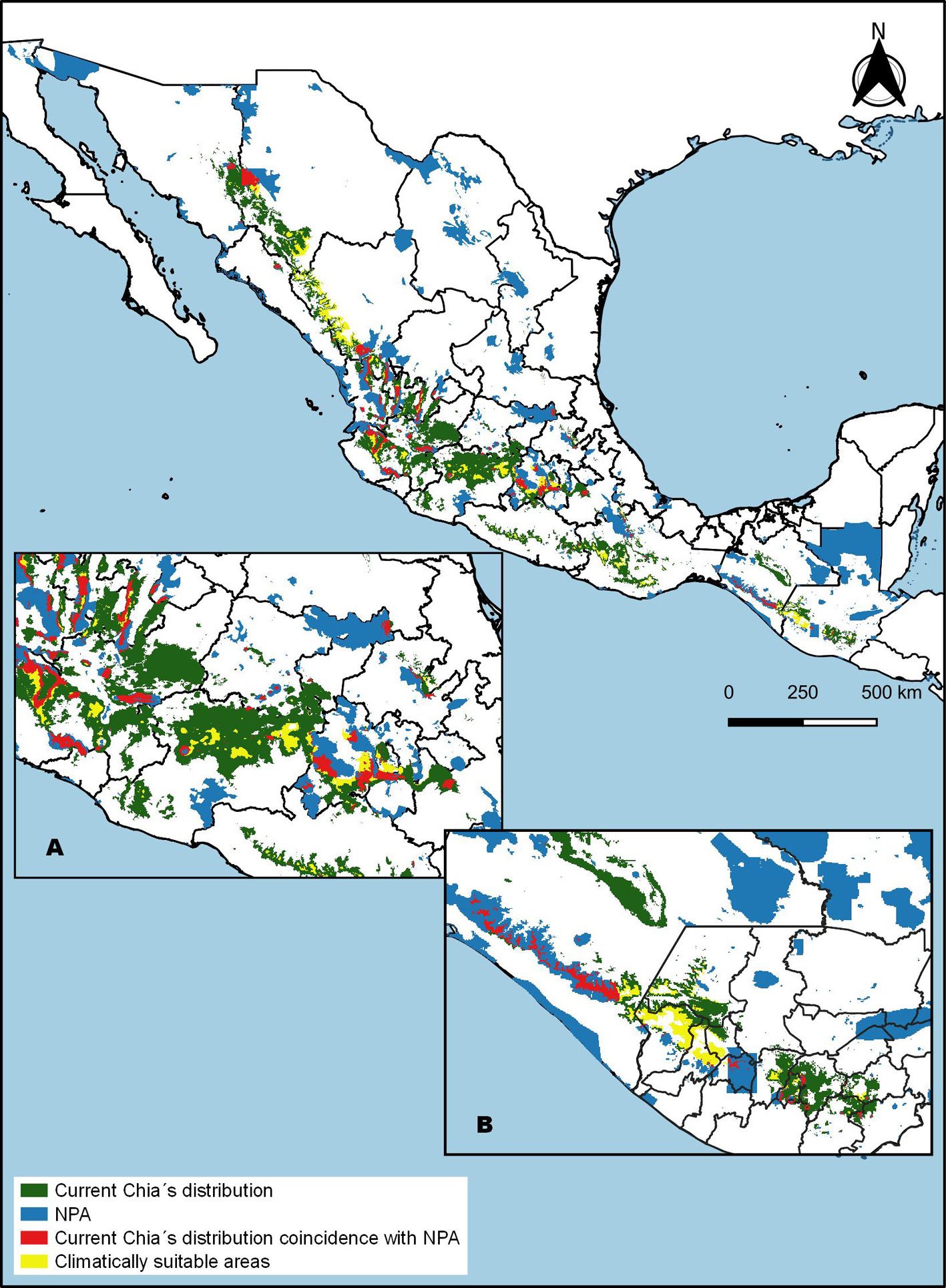
Finally, the climatically stable area suitable for S. hispanica was estimated to be 32,245 km², representing only 16.72% of its total current distribution area (Fig. 3). In Mexico, these stable areas (representing 15.5% of total estimated sites) are located primarily in the northwest (states of Chihuahua and Durango), west (Jalisco and Michoacán), central south (Estado de México, Mexico City, and Guerrero), and southern regions (Oaxaca and Chiapas).
| Variable | SSP2-4.5 (Optimistic scenario) | SSP5-8.5 (Pessimistic scenario) | ||||
|---|---|---|---|---|---|---|
| 2040 | 2060 | 2080 | 2040 | 2060 | 2080 | |
| bio 1 Annual mean temperature (°C) | +1.61 | +2.71 | +4.15 | +1.61 | +2.71 | +4.17 |
| bio 2 Mean diurnal range (mean of monthly (max temp − min temp)) (°C) | +0.07 | +0.21 | +0.41 | +0.07 | +0.20 | +0.41 |
| bio 3 Isothermality (BIO2 / BIO7) (× 100) | -0.55 | -0.76 | -0.89 | -0.55 | -0.78 | -0.91 |
| bio 4 Temperature seasonality (standard deviation × 100) | -1.65 | +0.59 | +4.50 | -1.71 | +0.45 | +4.20 |
| bio 5 Max temperature of warmest month (°C) | +1.84 | +3.13 | +4.77 | +1.83 | +3.14 | +4.78 |
| bio 6 Min temperature of coldest month (°C) | +1.49 | +2.49 | +3.78 | +1.49 | +2.49 | +3.78 |
| bio 7 Temperature annual range (BIO5−BIO6) (°C) | +0.34 | +0.64 | +0.99 | +0.34 | +0.64 | +1.00 |
| bio 10 Mean temperature of warmest quarter (°C) | +1.58 | +2.73 | +4.20 | +1.58 | +2.72 | +4.20 |
| bio 11 Mean temperature of coldest quarter (°C) | +1.62 | +2.70 | +4.09 | +1.62 | +2.71 | +4.11 |
| bio 12 Annual precipitation (mm) | +33.97 | +27.62 | +9.77 | +34.76 | +29.44 | +11.39 |
| bio 13 Precipitation of wettest month (mm) | +16.74 | +16.39 | +12.97 | +16.93 | +16.88 | +14.36 |
| bio 14 Precipitation of driest month (mm) | -0.10 | -0.38 | -0.66 | -0.10 | -0.40 | -0.72 |
| bio 15 Precipitation seasonality (coefficient of variation) (%) | +2.10 | +2.41 | +2.64 | +2.14 | +2.53 | +2.91 |
| bio 16 Precipitation of wettest quarter (mm) | +22.52 | +18.74 | +2.34 | +23.28 | +20.44 | +4.86 |
| bio 17 Precipitation of driest quarter (mm) | -0.92 | -1.95 | -3.18 | -0.93 | -2.00 | -3.31 |
| Climatically stable areas in km² | 32,245 | |||||
| % | 16.72 | |||||
Discussion
Here we report a concerning scenario for the persistence of wild chia populations in the face of global warming through a Species Distribution pipeline employed in Maxtent. Although other pipelines are available such as the use of Random Forests (Breiman, 2001), we were unable to employ it because it requires an even number both of species presences and species absences, which is difficult since usually the latter is many folds larger than the number of presences (Gómez-Pineda et al., 2020). Nevertheless, our resulting hypotheses are robust following current scientific criteria and could serve as a starting point to guide conservation of this CWR for in field follow up to monitor wild chia populations, to reassess proposed abiotic variables and soil interacting agents to fine tune critical variables, and to enhance hypotheses and assure assisted migration success if implemented. Climate change poses imminent threats to individuals, species, and ecosystems (Kaeslin et al., 2012), and the conservation of CWRs is directly linked to future food security. The projected future distribution scenarios for 2040, 2060, and 2080 indicate a dramatic decline in the extent of suitable habitats for wild chia populations; even under the most optimistic scenario area loss is projected. We also foresee a geographic shift in the species’ average longitude and latitude climatic niche, along with a sharp net contraction in elevational range, where the lower elevation limit of the current natural range is expected to suffer larger losses; this finding agrees with projections for many other wild plant species through Mexican mountain gradients (Ramírez-Barahona et al., 2025). The speed of climatic change, exacerbated by the current acceleration of this process (Hansen et al., 2025), makes it highly unlikely that natural populations could disperse their seeds and establish new populations at the locations where suitable climatic conditions will emerge at the required pace. In other words, the mismatch between the areas currently occupied by wild populations and the shifting climate suitable for them will increase over time. Human-assisted translocation of seeds would likely be necessary to ensure species persistence. On the other hand, so-called “climatically stable” areas should not be interpreted with undue optimism. The persistence of an area within the species’ overall climatic niche does not imply that local conditions remain unchanged. This distinction is important when considering populations with significant genetic differentiation in traits such as frost resistance or drought tolerance. Specific populations may remain within the species’ broad climatic niche but become uncoupled from the narrow climate interval to which they have evolved and specialized, as demonstrated for wild forest tree populations along environmental gradients (Ortiz-Bibian et al., 2017; Rehfeldt et al., 2018). All these results add S. hispanica to the growing list of CWRs at risk. For instance, Jarvis et al. (2008) projected climate change effects on the conservation of wild relatives of peanuts (Arachis), potato (Solanum), and cowpea (Vigna), emphasizing the urgency of preserving their natural habitats and, in extreme cases, collecting and storing their genetic material in germplasm banks. Alarmingly, wild populations in the Trans-Mexican Volcanic Belt, a region of highest reported genetic diversity for chia (Cahill, 2004), are expected to be completely lost. Our global climate change scenarios differ markedly from those reported by Durán et al. (2016), who projected an increase in the potential distribution of S. hispanica (chia) under future climate conditions. Overall, they interpreted global climate change as potentially beneficial for the species, predicting moderate to high environmental suitability for 2060 and 2080, and an expansion of suitable areas across central and southern Mexico (Durán et al., 2016). Direct comparison between both studies is difficult due to several methodological differences, including the source of occurrence records (wild-only vs. potentially mixed wild and cultivated), variation in raster resolution (2.5 arc-minutes vs. our 30 arc-seconds), and differences in environmental variables. While we relied solely on bioclimatic variables from WorldClim, Durán et al. (2016) supplemented these data with elevational information from SIAN (translated as Environmental Information System) at INIFAP (National Institute of Forestry, Agriculture and Livestock Research) and photoperiod. Unlike Durán et al. (2016), we did not include elevation. Elevation could be considered a surrogated variable of Mean Annual Temperatures and related temperature variables. There is a strong correlation between temperature and elevation along elevational gradients, at a lapse rate of approximately 0.5 oC for each 100 m of elevational difference (Sáenz-Romero et al., 2010). However, when the species has extensive latitudinal distribution (as in this case) the correlation temperature-elevation will vary and thus, adding elevation as an environmental variable could have confounded effects. Nonetheless, both studies converge in predicting habitat loss in northeastern Mexico, and project similar temperature increases: Durán et al. (2016) estimated an average temperature rise of 1 to 3 oC, while our models predict an average temperature increase of 2.28 oC, ranging from 1.61 to 4.16 oC over the average. Additionally, our projections indicate a mean annual precipitation increase, although it is extremely important to realize that such change has a strong seasonal component. Actual precipitation increase is projected only for the wettest quarter; meanwhile, there is a net decrease of precipitation in all the other quarters. Thus, the total annual precipitation increase is not necessarily beneficial for the biology of the species, since the dry season becomes both drier and warmer. The balance between temperature and rainfall variables are critical for the species’ survival and ecological performance (Böhning-Gaese et al., 2008; Uribe, 2015). Although our study focused exclusively on wild populations of chia as a CWR, it is relevant to note that projections for chia cultivation in Mexico by 2040-2069 (Orozco de Rosas et al., 2014) predict an expansion of suitable areas, particularly in the highlands of Sinaloa, Nuevo León, Tamaulipas, Veracruz, Nayarit, Jalisco, Michoacán, Guerrero, Oaxaca, Morelos, Puebla, and Chiapas. These findings do not contradict our results, as they reflect different environmental requirements between wild and cultivated chia (Chen et al., 2017). Unfortunately, if the CWRs are lost, new characters would not be available to transfer into the cultivars, as has been the case in other crops, such as resistance to pests [from Solanum demissum Lindl. (Díaz-García et al., 2023) to potatoes; from Solanum peruvianum L., Solanum cheesmanii (L.Riley) Fosberg, and Solanum pennellii Correll to tomatoes (Rick & Chetelat, 1995)]; cytoplasmic male sterility in sunflowers (Hajjar & Hodgkin, 2007); and tolerance to drought and salinity in tomatoes (Solanum chilense (Dunal) Reiche and S. pennellii (Rick & Chetelat, 1995) among other traits (see Hajjar & Hodgkin, 2007 for further information). To date, most breeding efforts in chia have focused on mutation induction via radiation (Jamboonsri et al., 2012; Sorondo, 2017), and the full potential of wild relatives remains largely unexplored. Although no severe pestrelated threats have yet been reported for chia cultivars, global warming is enabling the emergence of new pests in many crops (Srinivasa et al., 2022), and chia may face similar risks in the near future. Therefore, we need to be prepared. For example, in Ghana, where chia is cultivated to alleviate hunger in low-income communities due to its low production costs and high nutritional value, several pest infections have already been reported, including coreid bugs (Lagria sp.), Zonocerus variegatus L., Diopsis macrophthalma Dalman (reported as the synonym Diopsis thoracica Westwood) and Fusarium wilt (Yeboah et al., 2014). In Mexico, chia’s center of origin, stem damage by Diabrotica speciosa (Germar), 1824 (Coleoptera) has been shown to reduce seed yield by up to 43% (Sosa-Baldivia & Ruiz-Ibarra, 2016). Interestingly, Salvia karwinskii Benth., a taxonomically close wild relative of chia, was reported to exhibit strong antifeedant activity against Spodoptera littoralis (Boisduval) and Diabrotica virgifera virgifera Leconti (Esquivel et al., 1996), highlighting the value of conserving wild taxa. Beyond climate change, other threats must be addressed to ensure effective in situ conservation of wild chia populations. Among these, land-use change related to anthropogenic activities is particularly severe and rapidly accelerating (Davison et al., 2021; Goettsch et al., 2021; Villaseñor et al., 2024). Although we were unable to model this factor directly, chia’s habitat loss has been documented since 2003 in regions such as Huehuetenango (Guatemala) and in the Mexican states of Jalisco, Colima, and Michoacán (Cahill, 2003) mainly due to overgrazing, land-use transformation to agricultural or residential, herbicide application in nearby monocultures, and induced or accidental burning (personal observations GOR). The current rates of habitat loss and degradation are even more dramatic, particularly due to transformation of pineoak woodlands, which are rich in Salvia species -other CWRs- (Cornejo-Tenorio & Ibarra-Manríquez, 2011; Lara-Cabrera et al., 2016). A hopeful sign is the overlap between the projected distribution of wild chia and existing conservation areas in Mesoamerica. As with other CWRs, these protected areas could serve as strongholds for in situ conservation (Tobón-Niedfeld et al., 2022). And although CWRs are not commonly used to define protected areas, they have been employed in specific cases, as in the establishment of the Sierra de Manantlán Biosphere Preserve to protect the corn wild relative Zea diploperennis (Guzmán & Iltis, 1991). New protected areas could be established to preserve the ca. 100 Mesoamerican CWRs threathened with extinction (Goettsch et al., 2021). Therefore, integrating CWR monitoring into conservation area management is a valuable recommendation (Vincent et al., 2022). Fortunately, wild chia currently occurs, and is expected to persist, within some of the most emblematic Biosphere Reserves in Mexico and Guatemala. We recommend in situ conservation managed by local communities, who have cultivated and utilized chia for over 3,000 years; this should be complemented by ex situ strategies, such as establishing germplasm banks that ensure adequate sampling of wild populations. However, access to this material must be regulated to protect local interests assuming The International Treaty on Plant Genetic Resources for Food and Agriculture (https://www. fao.org/plant-treaty/overview/text-treaty/en). Also, ex situ conservation could involve cultivating wild populations in areas projected to remain suitable or those that would emerge as new suitable areas (in general at higher elevations than today) under future climate scenarios, as proposed for other rare and endangered Mexican plant species (Mendoza-Maya et al., 2022).
Acknowledgements
The first author acknowledges financing through the Secretaría de Ciencias, Humanidades, Tecnología e Innovación: Project 319466; Coordinación de la Investigación Científica, Universidad Michoacana de San Nicolás de Hidalgo. We also thank Joseph Cahill for access to his data set, Yocupitzia Ramírez Amezcua for fruitful discussions, Pedro Chamu for plant collections, and Geraldine Murillo and David Lomeli who participated in data set depuration.
References
Akaike, H. (1974). A new look at the statistical model identification. In IEEE Transactions on Automatic Control, 19, 716–723. https://doi.org/10.1109/TAC.1974.1100705
Ali, N. M., Yeap, S. K., Ho, W. Y., Beh, B. K., Tan, S. W., & Tan, S. G. (2012). The promising future of chia, Salvia hispanica L. Journal of Biomedicine and Biotechnology, 2012, 171956. https://doi.org/10.1155/2012/171956
Alkishe, A. A., Peterson, A. T., & Samy, A. M. (2017). Climate change influences on the potential geographic distribution of the disease vector tick Ixodes ricinus. Plos One, 12, e0189092. https://doi.org/10.1371/journal.pone.0189092
Anderson, R., Lew, D., & Peterson, A. T. (2003). Evaluating predictive models of species distributions: criteria for selecting optimal models. Ecological Modelling, 162, 211–232. https://doi.org/10.1016/S0304-3800(02)00349-6
Anuario Estadístico de Producción Agrícola. (2025). Servicio de información Agroalimentaria y Pesquera. Gobierno de México. Retrieved June 12, 2025 from: https://nube.agricultura.gob.mx/cierre_agricola/
Atauchi, P. J., Aucca-Chutas, C., Ferro, G., & Prieto-Torres, D. A. (2020). Present and future potential distribution of the endangered Anairetes alpinus (Passeriformes: Tyrannidae) under global climate change scenarios. Journal of Ornithology, 161, 723–738. https://doi.org/10.1007/s10336-020-01762-z
Barve, N., & Barve, V. (2016). ENMGadgets: tools for pre and post processing in ENM workflow. R package version 0.0.14. Available from: https://github.com/narayanibarve/ENMGadgets
Barve, N., Barve, V., Jiménez-Valverde, A., Lira-Noriega, A., Maher, S. P., Peterson, A. T. et al. (2011). The crucial role of the accessible area in ecological niche modeling and species distribution modeling. Ecological Modelling, 222, 1810–1819. https://doi.org/10.1016/j.ecolmodel.2011.02.011
Bi, D., Dix, M., Marsland, S., O’Farrell, S., Rashid, H., Uotila, P. et al. (2013). The ACCESS coupled model: description, control climate and evaluation. Australian Meteorological and Oceanographic Journal, 63, 41–64. https://doi.org/10.1071/ES13004
Böhning-Gaese, K., Jetz, W., & Schaefer, H. C. (2008). Impact of climate change on migratory birds: community reassembly versus. Global Ecology and Biogeography, 17, 38–49. https://doi.org/10.1111/j.1466-8238.2007.00341.x
Booth, T. H. (2022). Checking bioclimatic variables that combine temperature and precipitation data before their use in species distribution models. Austral Ecology, 47, 1506–1514. https://doi.org/10.1111/aec.13234
Boria, R. A., Olson, L. E., Goodman, S. M., & Anderson, R. P. (2014). Spatial filtering to reduce sampling bias can improve the performance of ecological niche models. Ecological Modelling, 275, 73–77. https://doi.org/10.1016/j.ecolmodel.2013.12.012
Bouman, F., & Meeuse, A. D. J. (2012). Dispersal in Labiatae. In R. M. Harley, & T. Reynolds (Eds.), Advances in Labiatae Science. Royal Botanic Gardens (pp. 193–202). Kew, UK.
Breiman, L. (2001). Random forests. Machine Learning, 45, 5–32. https://doi.org/10.1023/A:1010933404324
Cahill, J. P. (2003). Ethnobotany of chia, Salvia hispanica L. (Lamiaceae). Economic Botany, 57, 604–618. https://doi.org/10.1663/0013-0001(2003)057[0604:EOCSHL]2.0.CO;2
Cahill, J. P. (2004). Genetic diversity among varieties of Chia (Salvia hispanica L.). Genetic Resources and Crop Evolution, 51, 773–781. https://doi.org/10.1023/B:GRES.0000034583.20407.80
Cahill, J. P. (2005). Human selection and domestication of chia (Salvia hispanica L.) Journal of Ethnobiology, 25, 155–174. https://doi.org/10.2993/0278-0771_2005_25_155_hsadoc_2.0.co_2
Calderón-Ruíz, A., Montes-Hernández, S., García-Perea, M. A., Covarrubias-Prieto, J., Aguirre-Mancilla, C. L., & Raya-Pérez, J. C. (2021). Caracterización de poblaciones de Chía silvestre y cultivada. Revista Mexicana de Ciencias Agrícolas, 12, 1161–1170. https://doi.org/10.29312/remexca.v12i7.2243
Chen, Y. H., Shapiro, L. R., Benrey, B., & Cibrián-Jaramillo, A. (2017). Back to the origin: in situ studies are needed to understand selection during crop diversification. Frontiers in Ecology and Evolution, 5, 125. https://doi.org/10.3389/fevo.2017.00125
Cheplick, G. P. (2022). Philomatry in plants: Why do so many species have limited seed dispersal? American Journal of Botany, 109, 29–45. https://doi.org/10.1002/ajb2.1791
Cobos, M. E., Peterson, A. T., Barve, N., & Osorio-Olvera, L. (2019). kuenm: an R package for detailed development of ecological niche models using Maxent. PeerJ, 7, e6281. https://doi.org/10.7717/peerj.6281
Cobos, M. E., & Bosch, R. A. (2018) Recent and future threats to the Endangered Cuban toad Peltophryne longinasus: potential additive impacts of climate change and habitat loss. Oryx, 52, 116–125. https://doi.org/10.1017/S0030605316000612
Collevatti, R. G., Terribile, L. C., de Oliveira, G., Lima-Ribeiro, M. S., Nabout, J. C., Rangel, T. F. et al. (2013). Drawbacks to palaeodistribution modeling: The case of South American seasonally dry forests. Journal of Biogeography, 40, 345–358. https://doi.org/10.1111/jbi.12005
Colunga-García Marín, P., & Zizumbo-Villarreal, D. (2004). Domestication of plants in Maya lowlands. Economic Botany, 58, S101-S110.
Contreras-Toledo, A. R., Cortés-Cruz, M. A., Costich, D., Rico-Arce, M De L., Brehm, J. M., & Maxted, N. (2018). A crop wild relative inventory for Mexico. Crop Science, 58, 1292–1305. https://doi.org/10.2135/cropsci2017.07.0452
Cornejo-Tenorio, G., & Ibarra-Manríquez, G. (2011). Diversidad y distribución del género Salvia (Lamiaceae) en Michoacán, México. Revista Mexicana de Biodiversidad, 82, 1279–1296.
Dantas, B. F., Moura, M. S. B., Pelacani, C. R., Angelotti, F., Taura, T. A., Oliveira, G. M. et al. (2020). Rainfall, not soil temperature, will limit the seed germination of dry forest species with climate change. Oecologia, 192, 529–541. https://doi.org/10.1007/s00442-019-04575-x
Davison, C. W., Rahbek, C., & Morueta-Holme, N. (2021). Land-use change and biodiversity: Challenges for assembling evidence on the greatest threat to nature. Global Change Biology, 27, 5414–5429. https://doi.org/10.1111/gcb.15846
Díaz-García, G., Enciso-Maldonado, G. A., & Lozoya-Saldaña, H. (2023). Solanum demissum Lindl. in potato breeding. Revista Chapingo. Serie Horticultura, 29, 131–148. https://doi.org/10.5154/r.rchsh.2023.01.001
Díaz-Vallejo, M., Peña-Peniche, A., Mota-Vargas, C., Piña-Torres, J., Valencia-Rodríguez, D., Rangel-Rivera, C. E. et al. (2024). Analyses of the variable selection using correlation methods: an approach to the importance of statistical inferences in the modeling process. Ecological Modelling, 498, 110893. https://doi.org/10.1016/j.ecolmodel.2024.110893
Dinerstein, E., Olson, D., Joshi, A., Vynne, C., Burgess, N. D., Wikramanayake, E. P. et al. (2017). An ecoregion-based approach to protecting half the terrestrial realm. Bioscience, 67, 534–545. https://doi.org/10.1093/biosci/bix014
Dormann, C. F., Elith, J., Bacher, S., Buchmann, C., Carl, G., Carré, G. et al. (2013). Collinearity: A review of methods to deal with it and a simulation study evaluating their performance. Ecography, 36, 027–046. https://doi.org/10.1111/j.1600-0587.2012.07348.x
Dupin, J., & Smith, S. D. (2019). Integrating historical biogeography and environmental niche evolution to understand the geographic distribution of Datureae. American Journal of Botany, 106, 667–678. https://doi.org/10.1002/ajb2.1281
Durán, N., Ruiz, J. A., González, D. R., Mena, S., & Orozco-de Rosas, G. (2016). Cambio climático y su impacto sobre la aptitud ambiental y distribución geográfica de Salvia hispanica L. en México. Interciencia, 41, 407–413.
Eamus, D., Boulain, N., Cleverly, J., & Breshears, D. D. (2013). Global change-type drought-induced tree mortality: Vapor pressure deficit is more important than temperature per se in causing decline in tree health. Ecology and Evolution, 3, 2711–2729.
Elith, J., Graham, C. H., Anderson, R. P., Dudík, M., Ferrier, S., Guisan, A. et al. (2006). Novel methods improve prediction of species’ distributions from occurrence data. Ecography, 29, 129–151. https://doi.org/10.1111/j.2006.0906-7590.04596.x
Elith, J. E., Phillips, S. J., Hastie, T., Dudík, M., Chee, Y. E., & Yates, C. J. (2011). A statistical explanation of Maxent for ecologists. Diversity and Distributions, 17, 43–57. https://doi.org/10.1111/j.1472-4642.2010.00725.x
Escobar, L. E., Lira-Noriega, A., Medina-Vogel, G., & Peterson, A. T. (2014). Potential for spread of the white-nose fungus (Pseudogymnoascus destructans) in the Americas: Use of Maxent and NicheA to assure strict model transference. Geospatial Health, 9, 221–229. https://doi.org/10.4081/gh.2014.19
Esquivel, B., Calderón, J. S., Sánchez, A. A., Ramamoorthy, T. P., Flores, E. A., & Domínguez, R. M. (1996). Recent advances in phytochemistry and biological activity of Mexican Labiatae. Revista Latinoamericana de Química, 24, 44–64.
Fick, S. E., & Hijmans, R. J. (2017). WorldClim 2: new 1 km spatial resolution climate surfaces for global land areas. International Journal of Climatology, 37, 4302–4315. https://doi.org/10.1002/joc.5086
Gama-Rodríguez, A. M., García, J. A., Lozano, L. F., & Prieto-Torres, D. A. (2024). Protecting breeding sites: a critical goal for the conservation of the golden eagle in Mexico under global change scenarios. Journal of Ornithology, 165, 1–17. https://doi.org/10.1007/s10336-024-02168-x
Goettsch, B., Urquiza-Haas, T., Koleff, P., Acevedo-Gasman, F., Aguilar-Meléndez, A., Alavez, V. et al. (2021). Extinction risk of Mesoamerican crop wild relatives. Plants, People, Planet, 3, 775–795. https://doi.org/10.1002/ppp3.10225
Gómez-Pineda, E., Sáenz-Romero, C., Ortega-Rodríguez, J. M., Blanco-García, A., Madrigal-Sánchez, X., Lindig-Cisneros, R. et al. (2020). Suitable climatic habitat changes for Mexican conifers along altitudinal gradients under climatic change scenarios. Ecological Applications, 30, e02041. https://doi.org/10.1002/eap.2041
Góral, P. (2025). Chia seeds market update – January 2025. Retrieved June 12, 2025.
Grancieri, M., Martino, H. S. D., & González-de Mejía, E. (2019). Chia seed (Salvia hispanica L.) as a source of proteins and bioactive peptides with health benefits: a review. Comprehensive Reviews in Food Science and Food Safety, 18, 480–499. https://doi.org/10.1111/1541-4337.12423
Guzmán, R., & Iltis, H. H. (1991) Biosphere reserve established in Mexico to protect rare maize relative. Diversity, 7, 82–84.
Hajjar, R., & Hodgkin, T. (2007). The use of wild relatives in crop improvement: a survey of developments over the last 20 years. Euphytica, 156, 1–13. https://doi.org/10.1007/s10681-007-9363-0
Hansen, J. E., Kharecha, P., Sato, M., Tselioudis, G., Kelly, J., Bauer, S. E. et al. (2025) Global warming has accelerated: Are the United Nations and the public well-informed? Environment: Science and Policy for Sustainable Development, 67, 6–44. https://doi.org/10.1080/00139157.2025.2434494
Hartmann, H., Bastos, A., Das, A. J., Esquivel-Muelbert, A., Hammond, W. M., Martínez-Vilalta, J. et al. (2022). Climate change risks to global forest health: emergence of unexpected events of elevated tree mortality worldwide. Annual Review of Plant Biology, 73, 673–702. https://doi.org/10.1146/annurev-arplant-102820-012804
Hanspach, J., Kühn, I., Schweiger, O., & Pompe, S. (2011). Geographical patterns in prediction errors of species distribution models. Global Ecology and Biogeography, 20, 779–788. https://doi.org/10.1111/j.1466-8238.2011.00649.x
Hewitt, G. M. (2004). Genetic consequences of climatic oscillations in the Quaternary. Philosophical Transactions of the Royal Society of London. Series B: Biological Sciences, 359, 183–195. https://doi.org/10.1098/rstb.2003.1388
Hijmans, R. J., Cameron, S. E., Parra, J. L., Jones, P. G., & Jarvis, A. (2005). Very high resolution interpolated climate surfaces for global land areas. International Journal of Climatology: A Journal of the Royal Meteorological Society, 25, 1965–1978. https://doi.org/10.1002/joc.1276
Hijmans, R. (2025). terra: spatial data analysis. R package version 1.8–55, https://rspatial.org/
Inman, J. (1835). Navigation and Nautical Astronomy for the use of British seamen. 3rd Edition. London: R. B. Bate.
Intergovernmental Panel on Climate Change. (2022). Climate Change 2022: Mitigation of Climate Change. Contribution of Working Group III to the Sixth Assessment Report of the Intergovernmental Panel on Climate Change. Geneva. Retrieved from https://www.ipcc.ch/report/sixth-assessment-report-working-group-3/
International Union for Conservation of Nature (IUCN) & United Nations Environment World Conservation Monitoring Centre (UNEP-WCMC). (2020). Protected planet-The latest initiative harnessing the world database on protected areas. The World Database on Protected Areas (WDPA). www.protectedplanet.net
Jamboonsri, W., Phillips, T. D., Geneve, R. L., Cahill, J. P., & Hildebrand, D. F. (2012). Extending the range of an ancient crop, Salvia hispanica L.-a new ω3 source. Genetic Resources and Crop Evolution, 59, 171–178. https://doi.org/10.1007/s10722-011-9673-x
Janeković, F., & Novak, T. (2012). PCA-A Powerful Method for Analyzing Ecological Niches. In P. Sanguansat (Ed.), Principal component analysis. Multidisciplinary applications (pp. 127–142) Croatia: InTech. https://doi.org/10.5772/38538
Jarvis, A., Lane, A., & Hijmans, R. J. (2008). The effect of climate change on crop wild relatives. Agriculture, Ecosystems & Environment, 126, 13–23. https://doi.org/10.1016/j.agee.2008.01.013
Jin, J., Jian, D., Zhou, X., Chen, Q., & Li, Y. (2025). Impact of El Niño —southern oscillation on global vegetation. Atmosphere, 16, 701. https://doi.org/10.3390/atmos16060701
Kaeslin, A., Redmond, I., & Dudley, N. (2012). Wildlife in a changing climate. FAO Forestry Paper, 167. Rome.
Katunzi-Kilewela, A., Kaale, L. D., Kibazohi, O., & Rweyemamu, L. M. (2021). Nutritional, health benefits and usage of chia seeds (Salvia hispanica): a review. African Journal of Food Science, 15, 48–59. https://doi.org/10.5897/AJFS2020.2015
Kirchhoff, P. (2000). Mesoamérica (Paul Kirchhoff). Dimensión Antropológica, 19, 15–32.
Klitgaard, B. B. (2012). Salvia. In G. Davidse, M. S. Sousa, S. Knapp, F. Chiang, & C. Ulloa (Eds.), Flora mesoamericana, Rubiaceae a Verbenaceae. Vol. 4, núm. 2 (pp. 147–245) Saint Louis: Missouri Botanical Garden Press.
Lara-Cabrera, S. I., Bedolla-García, B. Y., Zamudio, S., & Domínguez-Vázquez, G. (2016). Diversidad de Lamiaceae en el estado de Michoacán, México. Acta Botanica Mexicana, 116, 107–149. https://doi.org/10.21829/abm116.2016.1120
Lara-Cabrera, S., Rivera, I., Aguilar, R., Farfán-Heredia, B., Orozco-de Rosas, G., Lomelí, D. et al. (2025). People and chia: a lengthy and bumpy relationship. In A. Casas, N. Peroni, F. Parra, V. S. Lema, X. Aguirre-Dugua, E. Arévalo-Marín et al. (Eds.), Biodiversity management and domestication in the Neotropics. Cham: Springer. https://doi.org/10.1007/978-3-031-64203-6_32-1
Legendre, P. (1993). Spatial autocorrelation: trouble or new paradigm? Ecology, 74, 1659–1673. https://doi.org/10.2307/1939924
Liu, J. P., Song, M., Horton, R. M., & Hu, Y. (2013). Reducing spread in climate model projections of a September ice-free Arctic. Proceedings of the National Academy of Sciences, 110, 12571–12576. https://doi.org/10.1073/pnas.1219716110
Marco, D. E., Montemurro, M. A., & Cannas, S. A. (2011). Comparing short and long-distance dispersal: modeling and field case studies. Ecography, 34, 671–682. https://doi.org/10.1111/j.1600-0587.2010.06477.x
Matrícula de Tributos (Edición Facsimilar). (2022). Arqueología Mexicana. Edición especial, 101. Ciudad de México. Editorial Raíces S.A. de C.V.
Maxted, N., Ford-Lloyd, B. V., Jury, S., Kell, S., & Scholten, M. (2006). Towards a definition of a crop wild relative. Biodiversity & Conservation, 15, 2673–2685. https://doi.org/10.1007/s10531-005-5409-6
Mendoza-Maya, E., Gómez-Pineda, E., Sáenz-Romero, C., Hernández, J. C., López-Sánchez, C. A., Vargas-Hernández, J. J. et al. (2022) Assisted migration and the rare endemic plant species: the case of two endangered Mexican spruces. PeerJ, 10, e13812. https://doi.org/10.7717/peerj.13812
Morrone, J. J., Escalante, T., & Rodríguez-Tapia, G. (2017). Provincias biogeográficas mexicanas: mapa y shapefiles. Zootaxa, 4277, 277–279. https://doi.org/10.11646/zootaxa.4277.2.8
Murrieta-Flores, P., Jiménez-Badillo, D., Martins, B., Favila-Vázquez, M., & Liceras-Garrido, R. (2020). DECM Machine Ready Corpus. T-AP Digging into Early Colonial Mexico Project. Figshare, Dataset. https://doi.org/10.6084/m9.figshare.12048729
Núñez-Landa, M. L., Montero-Castro, J. C. M., Monterrubio-Rico, T. C., Lara-Cabrera, S. I., & Prieto-Torres, D. A. (2023). Predicting co-distribution patterns of parrots and woody plants under global changes: the case of the Lilac-crowned Amazon and Neotropical dry forests. Journal for Nature Conservation, 71, 126323. https://doi.org/10.1016/j.jnc.2022.126323
Orozco-de Rosas, G., Durán-Puga, N., González-Eguiarte, D. R., Zarazúa-Villaseñor, P., Ramírez-Ojeda, G., & Mena-Munguía, S. (2014). Proyecciones de cambio climático y potencial productivo para Salvia hispanica L. en las zonas agrícolas de México. Revista Mexicana de Ciencias Agrícolas, 5, 1831–1842.
Ortiz-Bibian, M. A., Blanco-García, A., Lindig-Cisneros, R. A., Gómez-Romero, M., Castellanos-Acuña, D., Herrerías-Diego, Y. et al. (2017). Genetic variation in Abies religiosa for quantitative traits and delineation of elevational and climatic zoning for maintaining Monarch Butterfly overwintering sites in Mexico, considering climatic change. Silvae Genetica, 66, 14–23. https://doi.org/10.1515/sg-2017-0003
Owens, H. L., Campbell, L. P., Dornak, L. L., Saupe, E. E., Barve, N., Soberón, J. et al. (2013). Constraints on interpretation of ecological niche models by limited environmental ranges on calibration areas. Ecological Modelling, 263, 10–18. https://doi.org/10.1016/j.ecolmodel.2013.04.011
Peterson, A. T., Cobos, M. E., & Jiménez-García, D. (2018). Major challenges for correlational ecological niche model projections to future climate conditions. Annals of the New York Academy of Sciences, 1429, 66–77. https://doi.org/10.1111/nyas.13873
Peterson, A. T., Ortega-Huerta, M. A., Bartley, J., Sánchez-Cordero, V., Soberón, J., Buddemeier, R. H. et al. (2002). Future projections for Mexican faunas under global climate change scenarios. Nature, 416, 626. https://doi.org/10.1038/416626a
Peterson, A. T., Papeş, M., & Soberón, J. (2008). Rethinking receiver operating characteristic analysis applications in ecological niche modeling. Ecological Modelling, 213, 63–72. https://doi.org/10.1016/j.ecolmodel.2007.11.008
Peterson, A. T., Soberón, J., Pearson, R. G., Anderson, R. P., Martínez-Meyer, E., Nakamura, M. et al. (2011). Ecological niches and geographic distributions (MPB-49). Princeton, NJ: Princeton University Press.
Phillips, S. J., Anderson, R. P., & Schapire, R. E. (2006). Maximum entropy modeling of species geographic distributions. Ecological Modelling, 190, 231–259. https://doi.org/10.1016/j.ecolmodel.2005.03.026
Prieto-Torres, D. A. (2024). Práctica 28. Adquisición y biocuración de datos distribucionales. In T. Escalante, E. A. García-Trejo, & J. J. Morrone (Eds.), Biogeografía práctica. (pp. 105–107) Ciudad de México: Facultad de Ciencias, Universidad Nacional Autónoma de México.
Prieto-Torres, D. A., Lira-Noriega, A., & Navarro-Sigüenza, A. G. (2020). Climate change promotes species loss and uneven modification of richness patterns in the avifauna associated to Neotropical seasonally dry forests. Perspectives in Ecology and Conservation, 18, 19–30. https://doi.org/10.1016/j.pecon.2020.01.002
Prieto-Torres, D. A., Núñez-Rosas, L. E., Remolina-Figueroa, D., & Arizmendi, M. C. (2021). Most Mexican hummingbirds lose under climate and land-use change: long-term conservation implications. Perspectives in Ecology and Conservation, 19, 487–499. https://doi.org/10.1016/j.pecon.2021.07.001
Ramamoorthy, T. P. (1996). Salvia. L. In G. Calderón-de Rzedowski, & J. Rzedowski (Eds.), Flora fanerogámica del Valle de México, 2a. Ed. (pp. 632–644). Instituto de Ecología, A.C. y Comisión Nacional para el Conocimiento y Uso de la Biodiversidad. Pátzcuaro, Michoacán.
Ramírez-Barahona, S., Cuervo-Robayo, Á. P., Feeley, K. J., Ortiz-Rodríguez, A. E., Vásquez-Aguilar, A. A., Ornelas, J. F. et al. (2025). Upslope plant species shifts in Mesoamerican cloud forests driven by climate and land use change. Science, 387, 1058–1063. https://www.science.org/doi/abs/10.1126/science.adn2559
Rehfeldt, G. E., Leites, L. P., Joyce, D. G., & Weiskittel, A. R. (2018). Role of population genetics in guiding ecological responses to climate. Global Change Biology, 24, 858–868. https://doi.org/10.1111/gcb.13883
Riahi, K., Van Vuuren, D. P., Kriegler, E., Edmonds, J., O’Neill, B. C., Fujimori, S. et al. (2017). The shared socioeconomic pathways and their energy, land use, and greenhouse gas emissions implications: an overview. Global Environmental Change, 42, 153–168. https://doi.org/10.1016/j.gloenvcha.2016.05.009
Rick, C. M., & Chetelat, R. T. (1995). Utilization of related wild species for tomato improvement. In I International Symposium on Solanacea for Fresh Market, 412, 21–38. https://doi.org/10.17660/ActaHortic.1995.412.1
Rödder, D., & Engler, J. O. (2011). Quantitative metrics of overlaps in Grinnellian niches: advances and possible drawbacks. Global Ecology and Biogeography, 20, 915–927. https://doi.org/10.1111/j.1466-8238.2011.00659.x
Rojas-Soto, O., Forero-Rodríguez, J. S., Galindo-Cruz, A., Mota-Vargas, C., Parra-Henao, K. D., Peña-Peniche, A. et al. (2024). Calibration areas in ecological niche and species distribution modeling: unravelling approaches and concepts. Journal of Biogeography, 51, 1416–1428. https://doi.org/10.1111/jbi.14834
Sáenz-Romero, C., Rehfeldt, G. E., Crookston, N. L., Duval, P., St-Amant, R., Beaulieu, J. et al. (2010). Spline models of contemporary, 2030, 2060 and 2090 climates for México and their use in understanding climate-change impacts on the vegetation. Climatic Change, 102, 595–623. https://www.fs.usda.gov/treesearch/pubs/36311
Soberón, J., & Peterson, A. T. (2005). Interpretation of models of fundamental ecological niches and species’ distributional areas. Biodiversity Informatics, 2, 1–10. https://doi.org/10.17161/bi.v2i0.4
Sorondo, A. (2017). U.S. Patent No. 9,686,926. Washington, DC: U.S. Patent and Trademark Office.
Sosa, A., Ruiz, G., Rana, J., Gordillo, G., West, H., Sharma, M. et al. (2016). Chia crop (Salvia hispanica L.): its history and importance as a source of polyunsaturated fatty acids omega-3 around the world: a review. Journal of Crop Research and Fertilizers, 1, 1–9.
Sosa-Baldivia, A., & Ruiz-Ibarra, G. (2016). ¿Será Diabrotica speciosa Germar, 1824 (Coleoptera: Chrysomelidae) una plaga de importancia económica para la producción de chía (Salvia hispanica L.) en México? Entomología Agrícola, 3, 269–274.
Srinivasa Rao, M., Mani, M., Prasad, Y. G., Prabhakar, M., Sridhar, V., Vennila, S. et al. (2022). Climate change and pest management strategies in horticultural and agricultural ecosystems. In M. Mani. (Ed) Trends in horticultural entomology (pp. 81–122). Springer, Singapore. https://doi.org/10.1007/978-981-19-0343-4_3
Stohlgren, T. J., Otsuki, Y., Villa, C. A., Lee, M., & Belnap, J. (2001). Patterns of plant invasions: a case example in native species hotspots and rare habitats. Biological Invasions, 3, 37–50. https://doi.org/10.1023/A:1011451417418
Terribile, L. C., Lima-Ribeiro, M. S., Araújo, M. B., Bizão, N., Collevatti, R. G., Dobrovolski, R. et al. (2012). Areas of climate stability of species ranges in the Brazilian Cerrado: disentangling uncertainties through time. Natureza & Conservação, 10, 152–159. https://doi.org/10.4322/natcon.2012.025
Tomlinson, S., Lewandrowski, W., Elliott, C. P., Miller, B. P., & Turner, S. R. (2020). High-resolution distribution modeling of a threatened short-range endemic plant informed by edaphic factors. Ecology and Evolution, 10, 763–777. https://doi.org/10.1002/ece3.5933
Tobón-Niedfeldt, W., Mastretta-Yanes, A., Urquiza-Haas, T., Goettsch, B., Cuervo-Robayo, A. P., Urquiza-Haas, T. et al. (2022). Incorporating evolutionary and threat processes into crop wild relatives conservation. Nature Communications, 13, 6254. https://doi.org/10.1038/s41467-022-33703-0
Uribe, B. E. (2015). El cambio climático y sus efectos en la biodiversidad en América Latina. Santiago: Comisión Económica para América Latina y el Caribe (CEPAL).
Velazco, S. J. E., Galvao, F., Villalobos, F., & De Marco, P. Jr. (2017). Using worldwide edaphic data to model plant species niches: an assessment at a continental extent. Plos One, 12, e0186025. https://doi.org/10.1371/journal.pone.0186025
Villaseñor, J. L., Ortiz, E., & Murguía-Romero, M. (2024). The rarest of rarities in the flora of Mexico. Botanical Sciences, 102, 1300–1317. https://doi.org/10.17129/botsci.3498
Vincent, H., Hole, D., & Maxted, N. (2022). Congruence between global crop wild relative hotspots and biodiversity hotspots. Biological Conservation, 265, 109432. https://doi.org/10.1016/j.biocon.2021.109432
Vincent, H., Wiersema, J., Kell, S., Fielder, H., Dobbie, S., Castañeda-Álvarez, N. P. et al. (2013). A prioritized crop wild relative inventory to help underpin global food security. Biological Conservation, 167, 265–275. https://doi.org/10.1016/j.biocon.2013.08.011
Watanabe, M., Suzuki, T., O’ishi, R., Komuro, Y., Watanabe, S., Emori, S. et al. (2010). Improved climate simulation by MIROC5: mean states, variability, and climate sensitivity. Journal of Climate, 23, 6312–6335. https://doi.org/10.1175/2010JCLI3679.1
Wei, T., & Simko, V. (2017). R package “corrplot”: Visualization of a correlation matrix. Retrieved. https://github.com/taiyun/corrplot
Wood, J. R. I., & Harley, R. M. (1989). The genus Salvia (Labiatae) in Colombia. Kew Bulletin, 44, 211–278.
Yeboah, S., Owusu-Danquah, E., Lamptey, J. N. L., Mochiah, M. B., Lamptey, S., Oteng-Darko, P. et al. (2014). Influence of planting methods and density on performance of chia (Salvia hispanica) and its suitability as an oilseed plant. Science and Education Centre of North America, 2, 14–26. http://dx.doi.org/10.12735/as.v2i4p14
Zelinka, M. D., Myers, T. A., McCoy, D. T., Po-Chedley, S., Caldwell, P. M., Ceppi, P. et al. (2020). Causes of higher climate sensitivity in CMIP6 models. Geophysical Research Letters, 47, e2019GL085782. https://doi.org/10.1029/2019GL085782
Zona, S. (2017). Fruit and seed dispersal of Salvia L. (Lamiaceae): a review of the evidence. The Botanical Review, 83, 195–212. https://doi.org/10.1007/s12229-017-9189-y