
Tania Escalante *, Leslie Madeline Elguea-Manrique, Perla Carolina Espíritu-Guerrero
Universidad Nacional Autónoma de México, Facultad de Ciencias, Departamento de Biología Evolutiva, Laboratorio Biogeografía de la Conservación, Circuito Exterior s/n, Ciudad Universitaria, Coyoacán, 04510 Ciudad de Mëxico, Mexico
*Corresponding author: tescalante@ciencias.unam.mx (T. Escalante)
Received: 27 July 2023; accepted: 5 March 2024
Abstract
The Transmexican Volcanic Belt (TVB) is a complex biogeographical province characterized by several areas of endemism and high diversity of flora and fauna produced by complex geological and evolutionary processes. Chorotypes are biogeographical patterns that occur either when 2 or more independently distributed species share the same occupied area, or even when a single species’ distribution area differs significantly from others. Here, we identified chorotypes of 167 endemic species inhabiting the TVB using geographic distribution models and quantitative methods. Of those species, 136 were included in 11 chorotypes, named I to XI. In addition, the insect Aedes niveoscotum constituted chorotype XII. The 30 remaining species did not belong to any chorotype. All chorotypes included species from different taxonomic groups, which may be due to a shared biogeographical history. The chorotypes with the highest richness were located in the central and eastern TVB, suggesting that volcano peaks and surrounding areas are important for generating the particular environmental conditions that restrict the distribution of species of different taxonomic groups.
Keywords: Biogeography; Patterns; Similarity; Species richness; Species distribution models
© 2024 Universidad Nacional Autónoma de México, Instituto de Biología. Este es un artículo Open Access bajo la licencia CC BY-NC-ND
(http://creativecommons.org/licenses/by-nc-nd/4.0/).
Corotipos y relaciones geográficas entre especies endémicas de la Faja Volcánica Transmexicana, México
Resumen
La Faja Volcánica Transmexicana (FVT) es una provincia biogeográfica compleja caracterizada por varias áreas de endemismo y una alta diversidad de flora y fauna, producto de complejos procesos geológicos y evolutivos. Los corotipos son patrones biogeográficos que ocurren cuando 2 o más especies de distribución independiente comparten la misma área de ocupación, o incluso cuando la distribución de una única especie difiere significativamente de otras. En este manuscrito, nosotras identificamos corotipos para 167 especies endémicas que habitan la FVT usando modelos de distribución geográfica y métodos cuantitativos. A partir del total de especies, 136 estuvieron incluidas en 11 corotipos, nombrados del I al XI. Adicionalmente, el insecto Aedes niveoscotum conformó el corotipo XII. Las 30 especies restantes no pertenecieron a ningún corotipo. Todos los corotipos incluyeron especies de diferentes grupos taxonómicos, lo cual puede deberse a una historia biogeográfica común. Los corotipos con la mayor riqueza de especies estuvieron localizados en el centro y este de la FVT, sugiriendo que los picos de los volcanes y las áreas circundantes son importantes para producir las condiciones ambientales particulares que restringen la distribución de las especies de diferentes grupos taxonómicos.
Palabras clave: Biogeografía; Patrones; Similitud; Riqueza de especies; Modelos de distribución de especies
Introduction
Distributional patterns in biogeography occur when a group of species share a given geographic space; while species that are distributed independently from each other show no distributional pattern (Márquez et al., 1997). The word “chorotype” was introduced by La Greca in 1963 (La Greca, 1963, in Morrone, 2014). According to Fattorini (2016), the term chorotype was implicitly used by La Greca to refer to “chorological categories”. Years later, an equivalence between chorological category and chorotype was established (Fattorini, 2016), defining a chorotype as the coincidence between the distribution ranges of species. Numerical chorotypes were defined by Baroni-Urbani et al. (1978) as a biogeographic pattern of 2 or more species occupying a similar area (Barbosa & Estrada, 2016; Real, Guerrero, & Vargas, 1992; Vargas & Real, 1997). Moreover, according to Real et al. (1996), the distribution area of a single species can be considered a chorotype if the distribution is significantly different from the distributions of other species. Because the identification of patterns using subjective methods can lead to mistaken results (Flores et al., 2004; Jardine, 1972; Márquez et al., 1997), it has been necessary to use quantitative techniques such as the appropriate similarity indices to produce coherent and reproducible results (Márquez et al., 1997). These techniques should compare the species’ distributions and their groupings in chorotypes (Barbosa & Estrada, 2016).
Similarity among species distributions has been analyzed from different perspectives. The Jaccard index (1908) has been used to compare the presence of species between 2 communities (Mostacedo & Fredericksen, 2000), but considers only presence data; it does not take into account the double absence of species. Real, Guerrero, and Ramírez (1992), and Real and Vargas (1996) consider this an advantage because the similarity between the 2 sites is not influenced by the number of other sites studied. However, Rice and Belland (1982) discussed that high or low values of Jaccard’s index could be random. Conversely, Baroni-Urbani and Buser (1976) proposed an index considering double absences, since 2 species could be absent from a locality due to ecological and historical reasons or inadequate sampling. Moreover, shared absences between species can be interpreted as coinciding distribution limits, like biogeographic barriers (Flores et al., 2004). For this index, there is a statistical table of associated probabilities (Baroni-Urbani & Buser, 1976). Later, Buser and Baroni-Urbani (1982) and Real, Guerrero, and Ramírez (1992) suggested caution in interpreting analyses that consider double absences, since including additional localities can alter the results of the index. Therefore, Real, Guerrero, & Vargas (1992) consider to Buser and Baroni-Urbani index as a feature of a relationship in the context of all the sites analyzed.
The Transmexican Volcanic Belt (TVB) is a complex mountainous biogeographical province between the Nearctic and Neotropical regions (Morrone et al., 2017). The TVB is located between 19-20° North latitude. It spans of 1,000 km and crosses Mexico in an east-west direction. This province is characterized by several areas of endemism and a high diversity of flora and fauna, produced by complex geological and biological processes (Hernández & Carrasco, 2007; Ruggiero & Ezcurra, 2003; Suárez-Mota et al., 2013). The TVB has the most heterogeneous relief and the highest elevations in Mexico, with important changes in altitude over short distances. This results in high climatic diversity between highland and lowland areas, which promotes high species richness (Hernández & Carrasco, 2007). The highest mountains in Mexico are in the TVB, including the Pico de Orizaba (5,650 m of altitude), Popocatépetl (5,450 m), Iztaccíhuatl (5,280 m), Nevado de Toluca (4,560 m), Malinche (4,460 m) and Nevado de Colima (4,340 m) (Suárez-Mota et al., 2013).
Non-random historical relationships could explain the biogeographic patterns displayed by the species of the TVB because they evolved under similar environmental conditions (Frey, 1992). Unfortunately, environmental deterioration resulting from the expansion of human activities has a negative effect on the habitat of many species distributed in the TVB. To contribute to the knowledge of biogeographical patterns in the TVB, we aimed to identify chorotypes of endemic species of 5 different taxa (amphibians, birds, insects, mammals and plants) using species distribution models and quantitative methods.
Materials and methods
We compiled a database of 167 endemic species of the TVB belonging to 5 taxonomic groups (Supplementary material: Table S1.1): 25 species of amphibians (Flores-Villela et al., 2010); 1 bird (Navarro-Sigüenza et al., 2003; Peterson et al., 2016); 89 species of insects (GBIF, 2017; Reyes-Castillo & Morón Ríos, 2005; SNIB-Conabio, 2017), 15 mammals (Escalante, 2015); and 37 plants (Magnoliopsida) (Escalante, 2015; Hernández & Gómez-Hinostrosa, 2011, 2015; Téllez-Valdés, 2017). These taxa were selected using their data points of occurrence from a previous database (Escalante et al., 2020; Supplementary material: Fig. S1.1), where at least 50% of the presence points for each species fell within the TVB polygon (Morrone et al., 2017).
To obtain the distribution areas of species, we generated species distribution models (SDM) for the 43 species with at least 6 data points using Maxent 3.4.0 (Phillips et al., 2017). SDM allow to predict the spatial distribution of a species based on statistical relationships between their occurrences and environmental conditions, producing a comprehensive understanding of the factors that molded species presence (Elith & Leathwick, 2009; Elith et al., 2006). The species distribution models were produced as in Escalante et al. (2020). Maxent was run using the ‘dismo’ package (Hijmans et al., 2017) in R version 3.4.2 (R Core Team, 2017) and we applied the omission error threshold of E = 10 (Peterson et al., 2008) to transform model output to binary. For the other 124 species (which had 5 or fewer data points or poor model performance), the geographic distribution was obtained directly from the data points.
Each species distribution model and geographic distribution was overlapped with a 0.5° latitude-longitude grid in QGIS v. 2.18.6 (QGIS Development Team, 2016) to determine the presence of a species in each cell of the grid. We built a presence-absence matrix for all species, where a species’ presence in each grid cell was coded as ‘1’ and absence as ‘0’. Based on the presence-absence matrix of 167 species and 609 cells, we applied the Baroni-Urbani and Buser index (1976) to obtain the similarity between the distributions of each pair of species. The index is as follows:

where A is the number of cells in which species “a” is present, B is the number of cells in which species “b” is present, C is the number of cells where both species “a” and “b” are present, and D is the number of cells in which both species “a” and “b” are absent. Because the double absences could lead to apparent similarity between 2 geographic distributions, they are multiplied by the double presences (Marquez et al., 1992). This could also prevent the effect of the Wallacean shortfall —i.e., lack of distribution data; Hortal et al., 2015— on some species, particularly those whose distributions were taken directly from points rather than modeled.
We identified chorotypes using the “Rmacoqui” package (Olivero et al., 2015) in R v.1.0.143 (R Core Team, 2017). Although all processes were developed in the R script, we describe the step-by step following: first, there was a transformation of the similarity matrix into a significant similarity matrix of ‘+’, ‘-’ and ‘0’ values, following to Márquez et al. (1997). Next, a cluster analysis was performed using the UPGMA (Unweighted Pair-Group Method using Arithmetic Averages) hierarchical classification method. For each cluster, we tested for significant segregation following McCoy et al. (1986). For each bifurcation in the dendrogram, a submatrix was developed, in which there are 3 zones with values that relate the species’ distributions: 1) “AxA zone”, including the values that related the “A group”; 2) “BxB zone”, which includes the values that related to the distributions of the “B group”; and 3) “AxB zone”, where the values related the “A group” with the “B group” distributions.
To evaluate whether the degree of similarity was higher than expected at random, we applied the DW parameter (McCoy et al., 1986). DW(AxA) quantifies the degree to which the major similarities (‘+’) are greater than expected at random in the “AxA zone”, but they are not in the “AxB zone”, at the same time that the minor similarities (‘-’) are absent from “AxA zone” (Real et al., 2003). DW(BxB) is analogous to DW(AxA), and both DW parameters contain all necessary conditions to determine whether A or B distributions belong to a chorotype. Therefore, we identified a chorotype when DW(AxA) and DW(BxB) were higher than 0.447 for all geographic distributions in the group (Real et al., 2003). Moreover, we applied the additional parameter GW to evaluate whether the segregation between the A and B groups was weak (Márquez et al., 1997). Finally, we calculated the DS parameter (Real et al., 2003), which determines whether the similarity was less than expected at random in the “AxB” zone, but not in the “AxA” and “BxB” zones, as well as whether higher-than-random similarities are absent in the “AxB” zone. The statistic test for DS was GS (McCoy et al., 1986). Therefore, a group was considered a chorotype if its DW was higher than ‘0’ and its corresponding statistic GW was significant.
In connection with that, we identified the least fuzzy chorotypical clusters, where all the conditions of a chorotype are maximized; however, a chorotypical cluster is neither true nor false, but accurate to some extent (Olivero et al., 2011). Moreover, certain fuzzy clusters may be nested within others, although it is always possible to identify the non-nested fuzzy chorotypes. Therefore, we applied the following fuzzy parameters to the least fuzzy chorotypes identified the degree of membership in the intersection between 2 chorotypes that indicates pairwise coincidences in the species membership (cardinality), and the fuzzy overlap that measures the proportion of the union that is in the intersection (Olivero et al., 2011).
Finally, we projected the grid and data points with the presence of each species for each chorotype using QGIS (QGIS Development Team, 2016) to locate each chorotype in the geographic space.
Results
We obtained a significant similarity matrix for the 167 species (available as Excel file in Supplementary material or through the e-mail of the authors). According to this matrix, 11 chorotypes from 136 species could be identified, hereafter referred to as chorotypes I through XI. Moreover, 1 insect species (A. niveoscotum) was significantly different from the rest and, therefore, was assigned to its own possible chorotype (chorotype XII). The richest chorotype was VII, with 39 species containing 23% of the total species analyzed. The chorotypes with the least species were X (with 4 species, 2.39% of the total richness) and XII (1 species, 0.59%) (Table 1). Eighteen percent of the species (30) were not included in any of the chorotypes.
Table 1.
Number of species from each taxonomic group belonging to each chorotype (I-XII), total species richness, and richness as a percentage of the total species considered. The species that were not included in any chorotype are in the last row.
| Chorotype | Number of species for each taxa | Richness | Richness percentage | ||||
| Amphibians | Bird | Insects | Mammals | Plants | |||
| I | 1 | 0 | 3 | 0 | 2 | 6 | 3.6 |
| II | 0 | 0 | 4 | 0 | 3 | 7 | 4.2 |
| III | 1 | 0 | 6 | 0 | 2 | 9 | 5.4 |
| IV | 2 | 0 | 11 | 0 | 1 | 14 | 8.4 |
| V | 1 | 0 | 7 | 0 | 1 | 9 | 5.4 |
| VI | 3 | 0 | 2 | 1 | 2 | 8 | 4.8 |
| VII | 6 | 1 | 11 | 7 | 14 | 39 | 23.3 |
| VIII | 1 | 0 | 5 | 0 | 0 | 6 | 3.6 |
| IX | 0 | 0 | 22 | 2 | 2 | 26 | 15.6 |
| X | 0 | 0 | 2 | 1 | 1 | 4 | 2.4 |
| XI | 0 | 0 | 6 | 0 | 2 | 8 | 4.8 |
| XII | 0 | 0 | 1 | 0 | 0 | 1 | 0.6 |
| Remaining species | 10 | 0 | 9 | 4 | 7 | 30 | 18 |

Figure 1. Simplified general dendrogram showing all chorotypes (I-XII). See figures S2.1 to S2.12 in Supplementary material to visualize in detail all the branches of each chorotype.
The general dendrogram included 12 sub-dendrograms, representing chorotypes I-XII (Fig. 1). All sub-dendrograms are shown in the Supplementary material (Figs. S2.1-S2.12). Chorotypes I, IV, VIII, and IX were located in the central and eastern part of the TVB (Figs. 2-4), chorotypes II, III, V and XI were located in the central TVB (Figs. 2, 3). Chorotype VI is located throughout the TVB, in the western, central and eastern parts (Fig. 3). In contrast to the rest, chorotype X was only in the eastern TVB (Fig. 5), and chorotype XII was located in the western TVB (Fig. 5).
Regarding the independence test GS, all species in chorotype IX had values above 0.5, except for species 95 (Aphodius ophistius), which had the lowest value (Supplementary material: Table S1.2). Chorotype XII had the highest membership value with a value of ‘1’ in the independence test. The fuzzy parameters that refer to including species within a chorotype are shown in Table 2, while the fuzzy overlap parameters are shown in Table 3. Inclusion (degree of integration in the intersection, likewise pairwise coincidences in the membership of the species) and overlap (which measures the proportion of the union that is found in the intersection) were related because the same chorotypic pairs had the highest values of both parameters (shown in bold; Tables 2, 3). In general, when we compared the inclusion values with the overlap values, we observed that the inclusion values were higher.
Discussion
We identified biogeographic patterns corresponding to chorotypes using the Baroni-Urbani and Buser (1976) index. The double absence component of this index was useful for our study area since the TVB has large mountain chains that have influenced species’ geographic distribution patterns. Consequently, geographic isolation could explain the absence or presence of different taxonomic groups in the TVB. In our particular dataset, the grouping of chorotypes was influenced by species distribution models versus individual data points, since using models generated larger chorotypes than the data points. These biases in data are named the Wallacean shortfall, defined as the lack of knowledge about the geographical distribution of the species (Hortal et al., 2015; Lomolino, 2004). Although in the last years have been published some contributions addressing how to deal with this shortfall (v. gr. Diniz-Filho et al., 2023), more research is necessary. As a result, we recommend that future analyses use only models or only data points for all species.

Figure 2. Cells of chorotypes I (3.6% of species richness), II (4.2%) and III (5.4%).
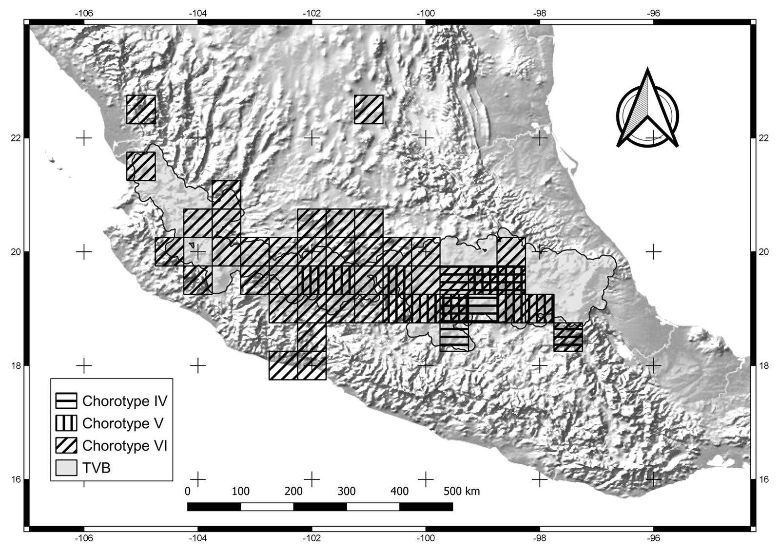
Figure 3. Cells of chorotypes IV (8.4% of species richness), V (5.4%) and VI (4.8%).
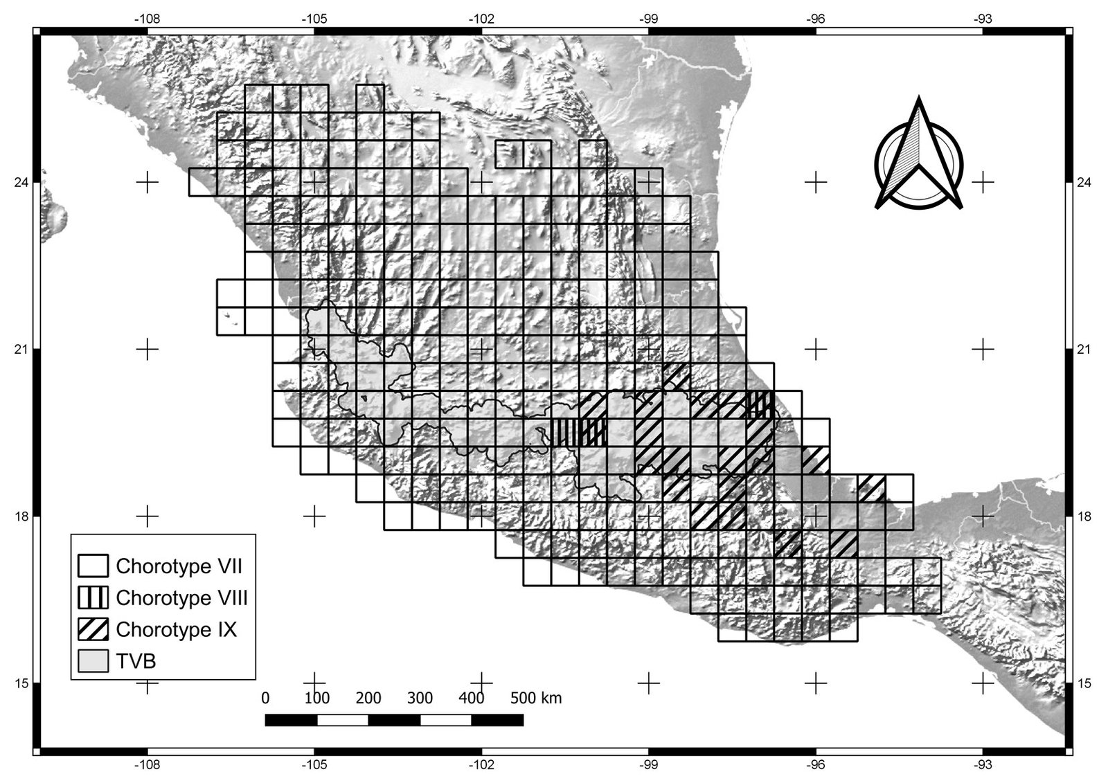
Figure 4. Cells of chorotypes VII (23.3% of species richness), VIII (3.4%) and IX (15.6%).
In general, similar analyses are generally performed within only one taxonomic group, e.g., amphibians (Flores et al., 2004; Olivero et al., 2011; Real, Guerrero, & Ramírez, 1992), plants (Gómez-González et al., 2004; Márquez et al., 1997), micro-mammals (Real et al., 2003) and birds (Real et al., 2008). Here, all 12 identified chorotypes included species from different taxonomic groups, which could be explained by similar geographic conditions resulting from a common biogeographic history of the species within a specific chorotype. Future analysis comparing other Operational Geographical Units and different scales could be necessary to evaluate the performance of the Baroni-Urbani and Buser (1976) index, which also could light about why some similar chorotypes are no grouped.
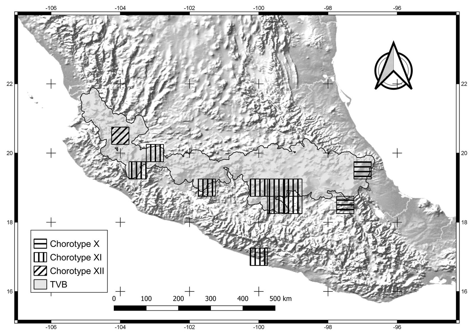
Figure 5. Cells of chorotypes X (2.4% of species richness), XI (4.8%) and XII (0.6%).
Table 2
Values that show the relationships between the chorotypes: inclusion of each chorotype regarding the rest according to cardinal parameter of fuzzy intersection between chorotypes. The bold numbers show the highest value in each column.
| Chorotypes | Values of relationship between chorotypes | |||||||||||
| CI (In) | CII (In) | CIII (In) | CIV (In) | CV (In) | CVI (In) | CVII (In) | CVIII (In) | CIX (In) | CX (In) | CXI (In) | CXII (In) | |
| CI | 1 | 0.720 | 0.803 | 0.718 | 0.742 | 0.635 | 0.595 | 0.572 | 0.580 | 0.744 | 0.697 | 0.467 |
| CII | 0.659 | 1 | 0.759 | 0.666 | 0.613 | 0.581 | 0.462 | 0.668 | 0.432 | 0.441 | 0.748 | 0.429 |
| CIII | 0.746 | 0.769 | 1 | 0.699 | 0.727 | 0.610 | 0.507 | 0.516 | 0.433 | 0.518 | 0.705 | 0.438 |
| CIV | 0.652 | 0.660 | 0.684 | 1 | 0.635 | 0.540 | 0.450 | 0.547 | 0.424 | 0.488 | 0.660 | 0.412 |
| CV | 0.605 | 0.546 | 0.639 | 0.571 | 1 | 0.663 | 0.515 | 0.537 | 0.429 | 0.566 | 0.694 | 0.484 |
| CVI | 0.417 | 0.416 | 0.431 | 0.390 | 0.534 | 1 | 0.500 | 0.541 | 0.336 | 0.432 | 0.566 | 0.688 |
| CVII | 0.679 | 0.576 | 0.623 | 0.566 | 0.721 | 0.869 | 1 | 0.600 | 0.540 | 0.733 | 0.725 | 0.626 |
| CVIII | 0.299 | 0.381 | 0.290 | 0.315 | 0.343 | 0.430 | 0.274 | 1 | 0.284 | 0.352 | 0.396 | 0.524 |
| CIX | 0.483 | 0.393 | 0.388 | 0.389 | 0.438 | 0.426 | 0.394 | 0.453 | 1 | 0.777 | 0.424 | 0.324 |
| CX | 0.307 | 0.199 | 0.230 | 0.222 | 0.286 | 0.272 | 0.265 | 0.278 | 0.385 | 1 | 0.245 | 0.277 |
| CXI | 0.406 | 0.475 | 0.442 | 0.423 | 0.495 | 0.502 | 0.370 | 0.442 | 0.296 | 0.345 | 1 | 0.480 |
| CXII | 0.029 | 0.029 | 0.029 | 0.028 | 0.037 | 0.065 | 0.034 | 0.062 | 0.024 | 0.042 | 0.051 | 1 |
Table 3
Values that show the relationships between the chorotypes: overlap between pairs of chorotypes according to cardinal parameters of fuzzy union between chorotypes. The bold numbers show the highest value in each column.
| Chorotypes | Values of relationship between chorotypes | |||||||||||
| CI | CII | CIII | CIV | CV | CVI | CVII | CVIII | CIX | CX | CXI | CXII | |
| CI | 1 | 0.524 | 0.631 | 0.519 | 0.500 | 0.337 | 0.464 | 0.244 | 0.358 | 0.278 | 0.345 | 0.028 |
| CII | 0.524 | 1 | 0.618 | 0.496 | 0.406 | 0.320 | 0.345 | 0.320 | 0.259 | 0.159 | 0.409 | 0.028 |
| CIII | 0.631 | 0.618 | 1 | 0.528 | 0.515 | 0.338 | 0.388 | 0.228 | 0.257 | 0.19 | 0.373 | 0.028 |
| CIV | 0.519 | 0.496 | 0.528 | 1 | 0.430 | 0.293 | 0.335 | 0.250 | 0.255 | 0.18 | 0.348 | 0.027 |
| CV | 0.5 | 0.406 | 0.515 | 0.43 | 1 | 0.420 | 0.429 | 0.265 | 0.277 | 0.235 | 0.406 | 0.035 |
| CVI | 0.337 | 0.32 | 0.338 | 0.293 | 0.420 | 1 | 0.465 | 0.315 | 0.231 | 0.2 | 0.363 | 0.063 |
| CVII | 0.464 | 0.345 | 0.388 | 0.335 | 0.429 | 0.465 | 1 | 0.232 | 0.295 | 0.242 | 0.325 | 0.033 |
| CVIII | 0.244 | 0.32 | 0.228 | 0.25 | 0.265 | 0.315 | 0.232 | 1 | 0.212 | 0.184 | 0.264 | 0.059 |
| CIX | 0.358 | 0.259 | 0.257 | 0.255 | 0.277 | 0.231 | 0.295 | 0.212 | 1 | 0.347 | 0.211 | 0.023 |
| CX | 0.278 | 0.159 | 0.19 | 0.18 | 0.235 | 0.200 | 0.242 | 0.184 | 0.347 | 1 | 0.167 | 0.038 |
| CXI | 0.345 | 0.409 | 0.373 | 0.348 | 0.406 | 0.363 | 0.325 | 0.264 | 0.211 | 0.167 | 1 | 0.049 |
| CXII | 0.028 | 0.028 | 0.028 | 0.027 | 0.035 | 0.063 | 0.033 | 0.059 | 0.023 | 0.038 | 0.049 | 1 |
Of the 167 species analyzed, 30 did not belong to any chorotype. In other words, they were distributed independently from other species which led to no significant distribution similarity with other species (Real et al., 2003). According to Real, Guerrero, and Vargas (1992), species not included in a chorotype have a random and independent distribution. The endemic species of amphibians, insects, mammals, and plants we included, in general, have very restricted geographical distribution in the TVB, due to geographical and ecological barriers (Hernández & Gómez-Hinostrosa, 2011). The species also had few data points, which in some cases could affect the inclusion of these species in a pattern.
Chorotypes I, IV, VII, and X are located in the central and eastern parts of the TVB. Similar geographic distribution patterns in the central and eastern TVB have been documented in the literature by Escalante et al. (2007), who identified an area of endemism for mammals in the eastern TVB. Chorotypes I, IV, VIII, and X also coincide with other patterns, probably related to the mountainous systems of the central and eastern part of the province, which have been considered players in important evolutionary events (Escalante et al., 2004; Morrone & Escalante, 2016).
Other chorotypes —II, III, IV and XI— show a similar distribution pattern in the central TVB. The central TVB has been highly studied because important volcanoes of Mexico are located there, including Popocatépetl, Iztaccíhuatl and the Nevado de Toluca, which have influenced species distributions. In particular, the Popocatépetl and Iztaccíhuatl volcanoes are located southeast of Mexico City, forming the Sierra Nevada (Almeida et al., 2007). The chorotypes located in the central region of the TVB show an affinity with the Sierra Ajusco-Chichinautzin (chorotypes II, III, and V) and Sierra Nevada Popocatépetl-Iztaccíhuatl (chorotypes III and V). Our chorotypes are similar to the pattern of endemic species of lagomorphs and rodents identified by Fa and Morales (1991). This finding suggests that volcano peaks and surrounding areas are important in generating the particular environmental conditions that restrict the distribution of species of different taxonomic groups (Alcántara & Paniagua, 2007). For example, Carex hermanni is a species of plant that is associated with the subalpine pine forest in the Popocatépetl-Iztaccíhuatl National Park, its immediate surroundings, and the slopes of the Sierra Nevada in Mexico State in the central TVB (Cochrane, 1981). C. hermanni is also linked to saturated soils, and different floristic combinations according to humidity and topography (Almeida et al., 2007). Another example is Ambystoma leorae, asalamander restricted to mountain streams of the pine forest of the Sierra Nevada, which have specific oxygenation and water temperature conditions (Sunny et al., 2014). Chorotype V is also located in the central TVB, occupying part of the Nevado de Toluca, with potential biotic relationships between its species.
Chorotype VI is a biogeographic pattern that coincides with the “Meridional TVB” region identified by Navarro-Sigüenza et al. (2007). These authors consider the influence of the main elevations in the biogeographic patterns in the central and eastern TVB (including the Popocatépetl, Iztaccíhuatl, Nevado de Toluca, and Malinche volcanoes) that spans central Mexico from Puebla to western Jalisco. The species of Chorotype VI (amphibians, insects, mammals and plants), may be influenced by varied environments due to the transition between the Balsas basin and mountainous and sub-mountainous environments (Navarro-Sigüenza et al., 2007).
The most extensive biogeographic pattern was Chorotype VII, which interestingly, is not restricted to the TVB. This pattern coincides with the Paleoamerican distribution pattern identified in insects by Halffter and Morrone (2017). Those authors explain the pattern as an ecological diversification of the oldest taxa of the TVB as follows: 1) these clades originally evolved in Eurasia or Africa and dispersed to the Americas during the Cretaceous-Paleocene; 2) the dispersal of those taxa occurred before and after the formation of the Mexican Plateau; and 3) they are adapted to highly different climatic conditions. The species belonging to chorotype VII are distributed throughout the Mexican Plateau, TVB, Sierra Madre Oriental and Occidental, and some tropical lowlands, showing a pattern that includes both tropical and temperate zones (Halffter & Morrone, 2017).
Chorotype IX occupies the southern Sierra Madre Oriental province (Morrone et al., 2017). This chorotype is located in the central-eastern TVB, at the boundary between the Sierra Madre del Sur and northwestern Oaxaca State. Chorotype IX coincides with the area of endemism 14 identified by Estrada et al. (2012), located in the Oaxaca-Tehuacanense province (Ramírez-Pulido & Castro-Campillo, 1990). This chorotype represents the geobiotic complexity of the distribution area of the species with a highly restricted distribution. For example, Neotoma nelsoni is a species of rodent distributed in the Pico de Orizaba and Cofre de Perote National Parks (González-Ruiz et al., 2006). Another species, Gentiana perpusilla (order: Gentianales, family: Gentianaceae), has a distribution that is restricted to the highlands of the State of Veracruz (Villareal et al., 2009). Also, the beetle Heliscus eclipticus shows a distribution in sub-humid and humid tropical forests and mountain cloud forests of Oaxaca, Puebla, and Veracruz (Villegas-Guzmán et al., 2012). Liebherr (1992) pointed out that the geological changes of the TVB have influenced the evolutionary history of species distributed in central Mexico, from the state of Puebla southward to Guerrero, Oaxaca, and Chiapas, as in the genus Platynus (order: Coleoptera, family: Carabidae). These geological changes may be related to volcanic successions of the TVB since its origin in the Miocene (Ferrusquía-Villafranca, 2007).
Chorotype XII comprises a single midge species, A. niveoscotum, distributed in Jalisco (Zavortink, 1972). This chorotype coincides with the biogeographic pattern found by García-Trejo et al. (2004). These authors explained the pattern due to the junction between the Sierra Madre Occidental and Sierra Madre del Sur. According to Darsie (1996), A. niveoscotum has an affinity to both the highlands (Nearctic) and lowlands (Neotropical) because this species may find adequate conditions for their survival and reproduction in this geographic area.
The chorotypes with high species richness and overlap values are distributed in the central and eastern TVB. These areas have been shown to have high richness of plants and animals by other authors (Alcántara & Paniagua, 2007; Escalante et al., 2007; Fa & Morales, 1991; Flores-Villela, 1993; Gámez et al., 2012; Llorente-Bousquets & Martínez, 1993) due to their geographic position, wide altitudinal ranges, and volcanic nature (Alcántara & Paniagua, 2007). This is important, according to Birks (1987), because chorotypic delimitation could be used to prioritize conservation strategies, where 2 aspects should be considered: high values of chorological overlap of the endemic biotic elements and areas where there is a high number of species. In addition, we recommend that future studies perform a correlation test between environmental variables and chorotype distribution to explain the importance of abiotic factors in the chorotypes, as well as other studies about the importance of ecological interactions.
In general, there are few publications about chorotypes, their methods of analysis, and case studies. Here, we present the first work identifying chorotypes in the Transmexican Volcanic Belt using different taxa, which resulted in 12 chorotypes. We could identify biogeographic patterns through chorotypes using both data points and species distribution models; however, the number of data points and models was decisive for inferring biogeographic patterns using the Baroni-Urbani and Buser index. Our chorotypes coincided with previously identified biogeographical patterns, mainly areas of endemism. The highest chorological overlap and species richness in the TVB is located in the central and eastern parts of the region, showing non-random close relationships of the species with the geographic space, probably resulting from ecological and evolutionary processes. These chorotypes could be an initial step in an integrative biogeographic protocol of the biota of the TVB.
Acknowledgements
This research was carried out with the support of the Program UNAM-DGAPA-PAPIIT, Project IN217717. The original databases were provided and processed by A. M. Varela-Anaya, E. A. Noguera-Urbano, L. M. Ochoa-Ochoa, A. L. Gutiérrez-Velázquez, P. Reyes-Castillo (deceased), H. M. Hernández, C. Gómez-Hinostrosa, A. G. Navarro-Sigüenza, O. Téllez-Valdés, I. Arenas Hidalgo, C. Miguel-Talonia and G. Pinilla-Buitrago. Lynna Kiere reviewed the English writing of this manuscript. We thank to two anonymous reviewers for their helpful comments.
References
Álcantara, O., & Paniagua, M. (2007). Patrones de distribución y conservación de plantas endémicas. In I. Luna, J. Morrone, J., & D. Espinosa-Organista (Eds.), Biodiversidad de la Faja Volcánica Transmexicana (pp. 421–438). Mexico City: UNAM.
Almeida-Leñero, L., Escamilla, M., Giménez-de Azcárate, J., González-Trápaga, A., & Cleef, A. (2007). Vegetación alpina de los volcanes Popocatépetl, Iztaccíhuatl y Nevado de Toluca. In I. Luna, J. Morrone, J., & D. Espinosa-Organista (Eds.), Biodiversidad de la Faja Volcánica Transmexicana (pp. 179–198). Mexico City: UNAM.
Barbosa, A. M. , & Estrada, A. (2016). Calcular corotipos sin dividir en OGUs: una adaptación de los índices de similitud para su utilización directa sobre áreas de distribución. In J. G. Zotano, J. Arias-García, J. A. Olmedo-Cobo, & J. L. Serrano-Montes (Eds.), Avances en biogeografía: áreas de distribución: entre puentes y barreras (pp. 157–163). Granada, Spain: Universidad de Granada/ Tundra Ediciones.
Baroni-Urbani, C., & Buser, M. (1976). Similarity of binary data. Systematic Zoology, 25, 251–259. https://doi.org/10.
2307/2412493
Baroni-Urbani, C., Ruffo, S., & Vigna-Taglianti, A. (1978). Materiali per una biogeografía italiana fondata su alcuni di Coleotteri Cicindelidi, Carabidi e Crisomelidi. Memoire della Societa Entomologica Italiana, 56, 35–92.
Birks, H. J. B. (1987). Recent methodological developments in quantitative descriptive biogeography. Annnales Zoologici Fennici, 24, 165–177.
Buser, M. W., & Baroni-Urbani, C. (1982). A direct nondimensional clustering method for binary data. Biometrics, 38, 351–360. https://doi.org/10.2307/2530449
Cochrane, T. (1981). Carex hermannii (Cyperaceae), a new species from Mexico, with comments on related species at high altitudes in Middle America. Brittonia, 33, 225–232. https://doi.org/10.2307/2806329
Darsie, J. (1996). A survey and bibliography of the mosquito fauna of Mexico (Diptera: Culicidae). Journal of the American Mosquito Control Association, 12, 298–306.
Diniz-Filho, J. F, Jardim, L., Guedes, J. J., Meyer, L., Stropp, J., Frateles, L. E. et al. (2023). Macroecological links between the Linnean, Wallacean, and Darwinian shortfalls. Frontiers of Biogeography, 15, e59566. http://dx.doi.org/10.21425/F5
FBG59566
Elith, J., Graham, C. H., Anderson, R. P., Dudík, M., Ferrier, S., Guisan, A. et al. (2006). Novel methods improve prediction of species’ distributions from occurrence data. Ecography, 29, 129–151. https://doi.org/10.1111/j.2006.0906-7590.04596.x
Elith, J., & Leathwick, J. R. (2009) Species distribution models: ecological explanation and prediction across space and time. Annual Review of Ecology, Evolution and Systematics, 40, 677–697. https://doi.org/10.1146/annurev.ecolsys.110308.120159
Escalante, T. (2015). Modelos de distribución de especies de mamíferos y suculentas de la Faja Volcánica Transmexicana. Mexico City: Facultad de Ciencias, Universidad Nacional Autónoma de México/ Data base SNIB-CONABIO Mamíferos, project JM055.
Escalante, T., Rodríguez, G., Gámez, N., León-Paniagua, L., Barrera, O., & Sánchez-Cordero, V. (2007). Biogeografía y conservación de los mamíferos. In I. Luna, J. J. Morrone y D. Espinosa (Eds.), Biodiversidad de la Faja Volcánica Transmexicana (pp. 485–502). Mexico City: UNAM.
Escalante, T., Rodríguez, G., & Morrone, J. J. (2004). The diversification of Nearctic mammals in the Mexican transition zone. Biological Journal of the Linnean Society, 83, 327-339. https://doi.org/10.1111/j.1095-8312.2004.00386.x
Escalante, T., Varela-Anaya, A. M., Noguera-Urbano, E. A., Elguea-Manrique, L., Ochoa-Ochoa, L. M., Gutiérrez-Velázquez, A. L. et al. (2020). Evaluation of five taxa as surrogates for conservation priorization in the Transmexican Volcanic Belt, Mexico. Journal for Nature Conservation, 54, 125800. https://doi.org/10.1016/j.jnc.2020.125800
Estrada, Y. Q., Luna, R. A., & Escalante, T. (2012). Patrones de distribución de los mamíferos en la provincia Oaxaca-Tehuacanense. Therya, 3, 33–51. https://doi.org/10.12933/therya-12-55
Fa, J., & Morales, L. (1991). Mammals and protected areas in the Trans-Mexican Neovolcanic Belt. In M. A. Mares, & D. J. Schmidly (Eds.), Latin American Mammalogy, history, biodiversity and conservation (pp. 199–226). Oklahoma: University of Oklahoma Press.
Fattorini, S. (2016). A history of chorological categories. History and Philosophy of the Life Sciences, 38, 12. https://doi.org/10.1007/s40656-016-0114-1
Ferrusquía-Villafranca, I. (2007). Ensayo sobre la caracterización y significación biológica. In I. Luna, J. J. Morrone, & D. Espinosa (Eds.), Biodiversidad de la Faja Volcánica Transmexicana (pp. 7–23). Mexico City: UNAM.
Flores, T., Puerto, M., Barbosa, A. M., Real, R., & Gosalvez, R. (2004). Agrupación en corotipos de los anfibios de la provincia de Ciudad Real (España). Revista Española de Herpetología, 24, 38–49.
Flores-Villela, O. (1993). Herpetofauna of Mexico: distribution and endemism. In T. P. Ramamoorthy, R. Bye, A. Lot y J. Fa (Eds.), Biological diversity of Mexico: origins and distribution (pp. 253–279). New York: Oxford University Press.
Flores-Villela, O., Canseco-Márquez, L., & Ochoa-Ochoa, L. (2010). Geographic distribution and conservation of the herpetofauna of the highlands of Central Mexico. In L. D. Wilson, J. H. Townsend, & J. D. Johnson (Eds.), Conservation of Mesoamerican amphibians and reptiles (pp. 302–321). Utah, USA: Eagle Mountain Publishing Co.
Frey, J. (1992). Response of a mammalian faunal element to climatic changes. Journal of Mammalogy, 73, 43–50. https://doi.org/10.2307/1381864
Gámez, N., Escalante, T., Rodríguez-Tapia, G., Linaje, M., & Morrone. J. J. (2012). Caracterización biogeográfica de la Faja Volcánica Transmexicana y análisis de los patrones de distribución de su mastofauna. Revista Mexicana de Biodiversidad, 83, 258–272. http://dx.doi.org/10.22201/ib.20078706e.2012.1.786
García-Trejo, E., & Navarro-Sigüenza, A. (2004). Patrones biogeográficos de la riqueza de especies y el endemismo de la avifauna en el oeste de México. Acta Zoológica Mexicana, 20, 167–185. https://doi.org/10.21829/azm.2004.2022336
Gómez-González, S., Cavieres, L., Teneb, E., & Arroyo, J. (2004). Biogeographical analysis of species of the tribe Cytiseae (Fabaceae) in the Iberian Peninsula and Balearic Islands. Journal of Biogeography, 31, 1659–1671. https://doi.org/10.1111/j.1365-2699.2004.01091.x
González-Ruiz, N., Ramírez-Pulido, J., & Genoways, H. (2006). Geographic distribution, taxonomy and conservation status of Nelson´s woodrat (Neotoma nelsoni) in Mexico. Southwestern Naturalist, 51, 112–116. https://doi.org/10.
1894/0038-4909(2006)51[112:GDTACS]2.0.CO;2
Halffter, G., & Morrone, J. J. (2017). An analytical review of Halffter´s Mexican Transition Zone, and its relevance for evolutionary biogeography, ecology and biogeographical regionalitation. Zootaxa, 4226, 1–46. https://doi.org/10.
11646/ZOOTAXA.4226.1.1
Hernández, H., & Gómez-Hinostrosa, C. (2011). Mapping the cacti of Mexico. Mexico City: Comisión Nacional para el Conocimiento y Uso de la Biodiversidad.
Hernández, H., & Gómez-Hinostrosa, C. (2015). Mapping the cacti of Mexico: Part II. Mexico City: Comisión Nacional para el Conocimiento y Uso de la Biodiversidad.
Hernández, M., & Carrasco, G. (2007). Rasgos climáticos más importantes. In I. Luna, J. J. Morrone y D. Espinosa (Eds.), Biodiversidad de la Faja Volcánica Transmexicana (pp. 57–72). Mexico City, México: UNAM
Hijmans, R., Phillips, S., Leathwick, J., & Elith, J. (2017). Package dismo: species distribution modeling. Retrieved on October 17th, 2017 from http://r.adu.org.za/web/packages/dismo/dismo.pdf
Hortal, J., de Bello, F., Diniz-Filho, J. A. F., Lewinsohn, T. M., Lobo, J. M., & Ladle, R. J. (2015). Seven shortfalls that beset large-scale knowledge of biodiversity. Annual Review of Ecology, Evolution and Systematics, 46, 523–549. https://doi.org/10.1146/annurev-ecolsys-112414-054400
Jaccard, P. (1908). Nouvelles recherches sur la distribution florale. Bulletin de la Societé Vauldoise des Sciences Naturelles, 44, 223–270.
Jardine, N. (1972). Computational methods in the study of plant distributions. In D. H. Valentine (Eds.), Taxonomy, phytogeography and evolution (pp. 381–393). London: Academic Press.
Liebherr, J. (1992). Phylogeny and revision of the Platynus dega-
llieri species group (Coleoptera, Carabidae, Platynini). Bulletin of the American Museum of Natural History, 214, 1–115.
Llorente-Bousquets, J., & Martínez, A. (1993). Analysis of Mexican butterflies: Papilionidae (Lepidoptera, Papilionoidea). In T. P. Ramamoorthy, R. Bye, A. Lot y J. Fa (Eds.), Biological diversity of Mexico: origins and distribution (pp. 147–178). New York, USA: Oxford University Press.
Lomolino M. V. (2004). Conservation biogeography. In M. V. Lomolino, & L. R. Heaney (Eds.), Frontiers of biogeography: new directions in the geography of nature (pp. 293–296). Sunderland, Massachusetts: Sinauer.
Márquez, A. L., Real, R., Vargas, J. M., & Salvo, A. E. (1997). On identifying common distribution patterns and their causal factors: a probabilistic method applied to pteridophytes in the Iberian Peninsula. Journal of Biogeography, 24, 613–631. https://doi.org/10.1111/j.1365-2699.1997.tb00073.x
McCoy, E. D., Bell, S. S., & Walters, K. (1986) Identifying biotic boundaries along environmental gradients. Ecology, 67, 749–759. https://doi.org/10.2307/1937698
Morrone, J. J. (2014) On biotas and their names. Systematics and Biodiversity, 12, 386–392. https://doi.org/10.1080/14772000.2014.942717
Morrone, J. J., & Escalante, T. (2016) Introducción a la biogeografía. Mexico City: UNAM.
Morrone, J. J., Escalante, T., & Rodríguez-Tapia, G. (2017). Mexican biogeographic provinces: map and shapefiles. Zootaxa, 4277, 277–279. https://doi.org/10.11646/zootaxa.
4277.2.8
Mostacedo, B., & Fredericksen, T. (2000). Manual de métodos básicos de muestreo y análisis en ecología vegetal. Santa Cruz, Bolivia: BOLFOR.
Navarro-Sigüenza, A., Peterson, A., & Gordillo-Martínez, A. (2003). Museums working together: The atlas of the birds of Mexico. Bulletin of the British Ornithologists’ Club, 116, 207–225.
Navarro-Sigüenza, A. G., Lira-Noriega, A., Peterson, A. T., Oliveras de Ita, A. & Gordillo-Martínez, A. (2007). Diversidad, endemismo y conservación de las aves. In I. Luna, J. J. Morrone, & D. Espinosa (Eds.), Biodiversidad de la Faja Volcánica Transmexicana (pp. 461–483). Mexico City: Comisión Nacional para el Conocimiento y Uso de la Biodiversidad/ Universidad Nacional Autónoma de México.
Olivero, J., Hidalgo, R., Márquez, A. L., Barbosa, A. M., & Real, R. (2015). R-Forge. Retrieved on December 1st, 2018 from http://rmacoqui.r-forge.r-project.org/RMacoqui-manual.pdf
Olivero, J., Real, R., & Márquez, A. L. (2011). Fuzzy chorotypes as a conceptual tool to improve insight into biogeographic patterns. Systematic Biology, 60, 645–660. https://doi.org/10.1093/sysbio/syr026
Peterson, A., Navarro-Sigüenza, A., & Gordillo-Martínez, A. (2016). The development of ornithology in Mexico and the importance of access to scientific information. Archives of Natural History, 43, 294–304. https://doi.org/10.3366/anh.2016.0385
Peterson, A. T., Papeş, M., & Soberón, J. (2008). Rethinking receiver operating characteristic analysis applications in ecological niche modeling. Ecological Modelling, 213, 63–72. https://doi.org/10.1016/j.ecolmodel.2007.11.008
Phillips, S., Anderson, R. P., Dudík, M., Schapire, R. E., & Blair, M. E. (2017). Opening the black box: an open-source release of Maxent. Ecography, 40, 887–893. https://doi.org/10.1111/ecog.03049
QGIS Development Team (2016). QGIS Geographic Information System. Retrieved on September 11th, 2017 from http://qgis.osgeo.org
R Core Team (2017). Rstudio: integrated development for R.Rstudio. Boston. Retrieved on November 20th, 2017 from http://www.rstudio.com
Ramírez-Pulido, J., & Castro-Campillo, A. (1990). Atlas Nacional de México. Provincias Mastofaunísticas. 1:4000000 Map IV. 8.8 A. Mexico City, UNAM.
Real, R., Guerrero, J. C., Márquez, A. L., Olivero, J., & Vargas, J. M. (2003). Tipificación corológica de los micromamíferos. Graellsia, 59, 287–298. https://doi.org/10.3989/graellsia.
2003.v59.i2-3.247
Real, R., Guerrero, J. C., & Ramírez, J. M. (1992). Identificación de fronteras bióticas significativas para los anfibios en la cuenca hidrográfica del sur de España. Doñana, Acta Vertebrata, 19, 53–70.
Real, R., Guerrero, J. C., & Vargas, J. M. (1992). Análisis biogeográfico de clasificación de áreas y especies. Monografías Herpetológicas, Asociación Herpetológica Española, 2, 73–84.
Real, R., Márquez, A. L., Guerrero, J. C., Vargas, J. M., & Palomo, L. J. (1996). Modelos de distribución de los insectívoros en la Península Ibérica. Doñana, Acta Vertebrata, 23, 123–142.
Real, R., Olivero, J., & Vargas, J. M. (2008). Using chorotypes to deconstruct biogeographical and biodiversity patterns: the case of breeding waterbirds in Europe. Global Ecology and Biogeography, 17, 735–746. https://doi.org/
10.1111/j.1466-8238.2008.00411.x
Real, R., & Vargas, J. M. (1996). The probabilistic basis of Jaccard’s index of similarity, Systematic Biology, 45, 380–385. https://doi.org/10.1093/sysbio/45.3.380
Reyes-Castillo, P., & Morón-Ríos, M. (2005). Passalidae y Lucanidae (Coleoptera: Scarabaeoidae) de México. Data base SNIB-CONABIO, projects AA014 and K005-Passalidae. Mexico City: Instituto de Ecología A.C.
Rice, J., & Belland, R. (1982). A simulation study of moss floras using Jaccard´s coefficient of similarity. Journal of Biogeography, 9, 411-419. https://doi.org/10.2307/2844573
Ruggiero, A., & Ezcurra, C. (2003). Regiones y transiciones biogeográficas: complementariedad de los análisis en biogeografía histórica y ecológica. In J. J. Morrone, & J. Llorente-Bousquets (Eds.), Una perspectiva lationoame-
ricana de la biogeografía (pp. 141–154). Mexico City: Las prensas de Ciencias, UNAM.
Suárez-Mota, M., Téllez-Valdéz, O., Lira-Saade, R., & Villaseñor, J. (2013). Una regionalización de la Faja Volcánica Transmexicana con base en su riqueza florística. Botanical Sciences, 91, 93–95. https://doi.org/10.17129/botsci.405
Sunny, A., Monroy-Vilchis, O., Reyna-Valencia, C., & Zarco-González, M. (2014). Microhabitat types promote the
genetic structure of a micro-endemic and critically endan-
gered mole salamander (Ambystoma leorae) of Central Mexico. Plos One, 9, e103595. https://doi.org/10.1371/journal.pone.0103595
Téllez, O. (2017). Distribución potencial de las especies Pina-
ceae (Pinus) y Fagaceae (Quercus) de México. Data base SNIB-CONABIO-Quercus, project JM010. Mexico City: Conabio.
Vargas, J. M., & Real, R. (1997). Biogeografía de los anfibios y reptiles de la Península Ibérica. In J. M. Pleguezuelos, & J. P. Martínez-Rica (Eds.), Distribución y biogeografía de los anfibios y reptiles de España y Portugal (pp. 309–320). Granada, Spain: Universidad de Granada/ Asociación Herpetológica Española.
Villarreal-Quintanilla, J., Estrada-Castillón, A., & Jasso-de Rodríguez, D. (2009). El género Gentiana (Gentianaceae) en México. Polibotánica, 27, 1–16.
Villegas-Guzmán, G., Francke, O., Pérez, T., & Reyes-Castillo, P. (2012). Coadaptación entre los ácaros (Arachnida: Klinckowstroemiidae) y coleópteros Passalidae (Insecta: Coleoptera). Revista de Biología Tropical, 60, 599–609. https://doi.org/10.15517/RBT.V60I2.3941
Zavortink, T. (1972). Mosquito studies (Diptera, Culicidae) XXVIII: The New World species formerly placed in Aedes (Finlaya). Contributions of the American Entomological Institute, 28, 1–206.


