Instituto del Mar del Perú, Sede Chimbote, Prolongación Los Pinos s/n Nueva Caleta Chimbote, Perú
*Autor para correspondencia: pberru@imarpe.gob.pe (P.M. Berrú-Paz)
Recibido: 25 enero 2024; aceptado: 23 octubre 2024
Resumen
Se identificó por primera vez en la región Ancash y el Perú, el cangrejo ermitaño Isocheles aequimanus (Dana, 1852), recolectado en las áreas de Mar Brava (09°16’57.39” S, 78°30’44.16” O) y Colorado (09°40’02.19” S, 78°19’21.59” O). Se describen sus caracteres taxonómicos y se analiza la asociación que existe con I. aequimanus y 8 conchas de gasterópodos (Nassarius dentifer, Polinices uber, Solatia buccionides, Stramonita biserialis, Thaissella chocolata, Trophon peruvianus, Xanthochorus buxea y Sinum cymba) que utiliza como habitáculo. Se estudiaron 231 ejemplares de I. aequimanus cuyas tallas variaron de 3.19 a 9.21 mm de longitud del escudo, con peso medio de 0.35 g. El 33.6% de los individuos fueron machos y 66.4% hembras. Las conchas de gasterópodos con mayor frecuencia de ocupación fueron N. dentifer con 59.7%, P. uber con 25.5%, S. buccionides con 6.9% y S. biserialis con 5.6%. Isocheles aequimanus se reporta como registro nuevo para las costas de Perú, incrementando el conocimiento de la riqueza específica de cangrejos ermitaños, promoviendo la necesidad de aumentar el esfuerzo en el estudio de la biodiversidad local y nacional, con el fin de cubrir vacíos informativos y establecer conexión geográfica con otros países de la región.
Palabras clave: Isocheles aequimanus; Cangrejo ermitaño; Conchas; Selección de conchas
Isocheles aequimanus (Paguroidea: Diogenidae), a new record of hermit crab for Peru, with bioecological observations in natural banks of Ensis macha
Abstract
The hermit crab Isocheles aequimanus (Dana, 182), was first identified in the Ancash region of Peru, specifically in the Mar Brava (09°16’57.39” S, 78°30’44.16” W) and Colorado (09°40’02.19” S, 78°19’21.59” W) areas. This study describes its taxonomic characteristics and analyzes the association between I. aequimanus and eight gastropod shells (Nassarius dentifer, Polinices uber, Solatia buccionides, Stramonita biserialis, Thaissella chocolata, Trophon peruvianus, Xanthochorus buxea, and Sinum cymba) used as shelter. Two-hundred and thirty-one specimens of I. aequimanus were analized, ranging in size from 3.19 to 9.21 mm shield length, with an average weight of 0.35 g. Of the analyzed individuals, 33.6% were males and 66.4% were females. The gastropod shells with the highest occupancy frequency were N. dentifer with 59.7%, P. uber with 25.5%, S. buccionides with 6.9%, and S. biserialis with 5.6%. Isocheles aequimanus is reported as a new record from the coasts of Peru, increasing the knowledge of the specific richness of hermit crabs, promoting the need to increase efforts in the study of local and nationalbiodiversity, in order to cover information gaps and establish geographic connections with other countries in the region.
Los cangrejos ermitaños de la familia Diogenidae se conocen comúnmente como cangrejos zurdos, por tener el quelípedo izquierdo generalmente más grande que el derecho (Bijukumar y Reshmi, 2018). Esta familia se identifica por no presentar un espacio en la parte basal del tercer maxilípedo (Ingle, 1992). Comprende 429 especies existentes, lo que representa la segunda familia más grande de cangrejos ermitaños marinos, después de Paguridae (McLaughlin et al., 2010). Dentro de esta familia se encuentra el género Isocheles (Stimpson, 1858) caracterizado por presentar los quelípedos iguales o subiguales, con los dactilos abriéndose en un plano generalmente horizontal (McLaughlin, 2003; Sánchez y Campos, 1978).
La forma de alimentarse puede darse captando partículas filtradas por las antenas, rastrillando la superficie de la arena con el tercer maxilípedo o utilizando las quelas para recoger alimento (Wicksten, 2012). Su distribución biogeográfica está restringida a aguas someras de las costas tropicales y subtropicales americanas (Mantelatto et al., 2006).
Vera-Silva y Mantelatto (2022) señalan que existen grandes similitudes entre las especies de este género, por ello, recientemente realizaron una actualización de la clave taxonómica basada en la forma y ornamentación de los quelípedos y del número de dientes ubicados en el segundo artículo de la antena, validando estos caracteres a nivel genético, y como resultado han sido descritas 6 especies en la actualidad: Isocheles aequimanus (Dana, 1852) en Chile, I. pilosus (Holmes, 1900) e I. wurdemanni (Stimpson, 1859) en Estados Unidos, I. pacificus (Bouvier, 1907) en México y Ecuador, I. sawayai (Forest y de Saint Laurent, 1968) en Venezuela y Brasil, e I. ingowehrtmanni (Vera-Silva y Mantelatto, 2022) en Costa Rica. En Perú, Moscoso (2013) reportó la presencia de I. pacificus caracterizándose por la terminación aguda en las puntas de los dedos del quelípedo, sin embargo, esta descripción no es un indicador taxonómico. En este estudio, se describe por vez primera a Isocheles aequimanus (Dana, 1852) para el litoral peruano y se analiza el patrón de ocupación de conchas de gasterópodos, asociadas al banco natural de Ensis macha en el submareal arenoso de las playas de Mar Brava y Colorado en la región Ancash.
Materiales y métodos
Los muestreos biológicos se realizaron en el submareal arenoso en las ensenadas de Mar Brava y Colorado, ubicadas en las provincias de El Santa y Casma, respectivamente, en la región Ancash (fig. 1a, b). Los ejemplares fueron recolectados manualmente en 4 estaciones, empleando como referencia un cuadrante de 1 m2, en el marco de las investigaciones propias que realiza el Laboratorio Costero de IMARPE Chimbote, durante julio del 2023.
Isocheles aequimanus fue identificado considerando principalmente: 1) la región dorsal y la forma del caparazón; 2) la forma y protuberancias en la vista dorsal de la quela izquierda; 3) el número de espinas en el segundo artículo de la antena izquierda en vista dorso mesial; y 4) la isometría de los quelípedos en forma y tamaño. La identificación específica se llevó a cabo utilizando las referencias bibliográficas de McLaughlin (2003), Guzmán (2004), Moscoso (2013) y Vera-Silva y Mantelatto (2022). Los especímenes están depositados en las colecciones del Instituto del Mar del Perú, sede Chimbote con el código IMARPE-LABCH 23-002.
Se registró como medida referencial la longitud del escudo, considerada como la máxima distancia entre el rostro y el borde medio posterior del escudo empleando un estereoscopio y un amplificador de imagen. Los especímenes fueron extraídos de sus conchas y dimensionados en las siguientes variables: longitud del escudo (LE) y peso total húmedo con una balanza analítica de 0.0001 gr de precisión; el sexo se determinó según Lancaster (1988), y con base en la presencia de gonoporos conspicuos en el sector basal (coxa) del tercer par de pereiópodos en las hembras y quinto par de pereiópodos en los machos, además de la presencia de huevos en las hembras.
Figura 1. Estaciones de muestreo del material biológico en las áreas de Mar Brava (a) y Colorado (b). Julio del 2023. Mapa elaborado por P.M. Berrú-Paz.
Con respecto de las conchas de gasterópodos usadas como refugios temporales, éstas fueron identificadas, medidas y pesadas considerando la talla de cada ejemplar de I. aequimanus hospedado en ellas. Las relaciones somatométricas se estimaron para confrontar pares de variables cuantitativas como longitud vs. peso total de I. aequimanus, longitud I. aequimanus vs. longitud de la concha, longitud I. aequimanus vs. peso de la concha, entre otras. El grado de coherencia entre estas variables se midió mediante el coeficiente de correlación de Pearson.
Resultados
Se estudiaron un total de 231 ejemplares de I. aequimanus, con medidas que variaron de 3.19 a 9.21 mm de longitud del escudo y con peso medio de 0.35 g. El 33.6% de los individuos analizados fueron machos y 66.4% hembras, de las cuales 82.2% correspondieron a hembras grávidas (tabla 1).
Tabla 1
Algunas variables biológicas registradas en Isocheles aequimanus en las playas de Mar Brava y Colorado en la región Áncash, julio de 2023.
Especie
N°
Rango (mm)
Talla (mm)
Peso (gr)
% ♂
% ♀
% ♀ ovig.
Isocheles aequimanus
231
3.19 – 9.21
4.31
0.35
33.6
66.4
82.8
Tabla 2
Dimensiones de conchas de gasterópodos empleadas como refugio por Isocheles aequimanus en las playas de Mar Brava y Colorado, junio de 2023.
Especie
N°
Rango (mm)
Talla (mm)
Peso (gr)
%
Nassarius dentifer
138
13.1 – 18.91
15.7
0.4
59.74
Polinices uber
59
11.7 – 25.72
16.8
1.3
25.54
Solatia buccinoides
16
15.3 – 24.88
18.8
0.6
6.93
Stramonita biserialis
13
18.7 – 28.63
22.8
1.8
5.63
Thaisella chocolata
2
21.2 – 37.13
29.2
4.2
0.87
Trophon peruvianus
1
31.4
31.4
1.8
0.43
Xanthochorus buxea
1
21.0
21.0
1.0
0.43
Sinun cymba
1
18.4
18.4
0.9
0.43
Total
231
Figura 2. Abundancia porcentual de la comunidad macro-bentónica en las áreas de estudio. Julio 2023.
La comunidad macrobentónica en las áreas de estudio estuvo representada por 27 taxones, de los cuales los crustáceos fueron los más abundantes con 62.25%, seguido por gasterópodos (13.28%), bivalvos (8.95%), poliquetos (3.61%) y otros (11.91%) (fig. 2). Dentro de los crustáceos, I. aequimanus correspondió al 97.3% de la abundancia, mientras que de los gasterópodos, Nassarius dentifer representó 80.8% de abundancia, y destacó la preferencia de I. aequimanus por las conchas de N. dentifer debido a la facilidad con que éstas se encuentran en el entorno.
Se identificaron 8 taxones de conchas de gasterópodos utilizadas como refugio por I. aequimanus, de los cuales N. dentifer (Powys, 1835), Polinices uber (Valenciennes, 1832), Solatia buccionoides (Sowerby, 1832) y Stramonita biserialis (Blainville, 1832) mostraron el mayor porcentaje de ocupación con 59.7, 25.5, 6.9 y 5.6%, respectivamente; mientras que Thaisella chocolata (Duclos, 1832), Trophon peruvianus (Lamarck, 1816), Xanthochorus buxeus (Broderip, 1833) y Sinum cymba (Menke, 1828) fueron los menos representados (tabla 2).
La macrofauna asociada al grupo gasterópoda estuvo representada por 5 especies, con abundancia numérica de 80.8% en N. dentifer, 15.1% en S. buccinoides, 1.7% en S. cymba, 1.4% en X. buxea y 1.0% en A. unifasciata (tabla 3).
Tabla 3
Diversidad de gasterópodos registrados como fauna asociada en las playas de Mar Brava y Colorado, junio de 2023.
Especie
N°
%
Nassarius dentifer
235
80.8
Solatia buccionoides
44
15.1
Sinum cymba
5
1.7
Xantochorus buxea
4
1.4
Alia unifasciata
3
1.0
Total
291
100
Diagnosis. Quelípedos de igual forma y tamaño, pilosos, con la superficie de color verde azulado en ejemplares vivos o frescos y anaranjados en individuos preservados con alcohol, presencia de tubérculos de diferentes tamaños distribuidos aleatoriamente (fig. 3).
Figura 3. Ejemplar macho (a) y hembra (b) de Isocheles aequimanus.
Márgenes laterales con espinas curvas de color dorado terminadas en el dedo fijo y móvil (fig. 4a). Segundo y tercer pereiópodo de gran tamaño a comparación del tercero y cuarto que son pequeños. Escudo más largo que ancho, con una coloración moteada entre azul, verde y gris, con presencia de mechones de setas largas y espinas pequeñas, proyecciones laterales terminadas con una espina (fig. 4b). Pedúnculo ocular de color azul grisáceo con pequeñas setas, una banda longitudinal de color marrón, córnea pequeña (fig. 4c). Acículos oculares con 3-4 espinas de color dorado (fig. 4d). Telson asimétrico, piloso, márgenes dorso laterales con espinas (fig. 4e). Urópodo izquierdo más grande que el derecho (fig. 4f).
Tabla 4
Valores medios de talla y peso de Isocheles aequimanus y distintos taxones de concha de gasterópodo habitada.
Paguridae
Talla (mm)
Peso (gr)
Concha gasterópodo
Talla (mm)
Peso (gr)
I. aequimanus
3.90
0.23
Nassarius dentifer
15.7
0.41
I. aequimanus
5.17
0.57
Polinices uber
16.8
1.27
I. aequimanus
4.14
0.32
Solatia buccinoides
18.7
0.67
I. aequimanus
5.11
0.56
Stramonita biserialis
22.8
1.79
I. aequimanus
6.88
0.39
Thaisella chocolata
29.2
4.23
I. aequimanus
4.33
0.37
Trophon peruvianus
31.4
1.76
I. aequimanus
3.64
0.18
Xantochorus buxea
21.0
0.96
I. aequimanus
5.73
0.34
Sinum cymba
18.4
0.92
Figura 4. Isocheles aequimanus: a) quelípedos, b) escudo, c) pedúnculo ocular, d) acículos oculares, e) telson y f) urópodos.
Figura 5. Indicadores taxonómicos de Isocheles aequimanus: a) quela izquierda con presencia de tubérculos; b) segundo artículo izquierdo de la antena con 6 espinas.
El análisis de los especímenes de Isocheles aequimanus concuerda con las características mencionadas en la redescripción de Vera-Silva y Mantelatto (2022). Como información adicional, I. aequimanus se diferencia de sus congéneres por la distribución de tubérculos en la superficie dorsal de la quela, con 3 filas más prominentes que otras (fig. 5a), y por la presencia de 6-8 espinas en el margen mesial del segundo artículo de la antena (fig. 5b).
Relaciones somatométricas. La correlación entre la talla media de I. aequimanus y las tallas y pesos de las distintas conchas de gasterópodos habitadas, permitió estimar una correlación positiva con valores de r2 de 0.7767 para talla vs. talla y de 0.9774 para talla vs. peso, lo que sugiere que los ejemplares de una talla determinada de I. aequimanus elijen proporcionalmente una talla y peso adecuado de la concha de gasterópodo a ocupar como refugio (tabla 4, fig. 6).
Figura 6. Curvas de correlación entre la talla de Isocheles aequimanus y talla (a) y peso (b) de distintos taxones de conchas de gasterópodos.
Figura 7. Correlación entre las variables talla y peso de Isocheles aequimanus.
Isocheles aequimanus vs. Nassarius dentifer. La correlación talla vs. peso, talla vs. talla y peso vs. peso entre I. aequimanus y concha de N. dentifer registró una asociación de tipo moderada con un coeficiente de correlación de Pearson estimado de 0.492, 0.481 y 0.436 para cada uno de los casos, respectivamente. En el caso de Polinices uber las correlaciones fueron más altas(0.791, 0.862 y 0.798, respectivamente); así como para Solatia buccionides (0.845, 0.630 y 0.770, respectivamente).
Relación longitud-peso. La relación longitud-peso en I. aequimanus permitió encontrar un buen ajuste al modelo potencial, con valores del coeficiente de determinación (r2) de 0.745, un valor de la pendiente “b” de 1.080 que denota un crecimiento alométrico negativo y un valor de la constante “a” de 0.0596 (fig. 7).
Discusión
En el submareal costero de la región Ancash (norte-centro del Perú) fue recolectada, identificada y registrada por primera vez la especie Isocheles aequimanus, como parte de la macrofauna acompañante durante el estudio de un recurso infaunal conocido como “navaja” Ensis macha, sin haber reportes hasta la fecha sobre otros estudios relacionados con su taxonomía y/o biología en el país.
En otros países, I. aequimanus fue revalidada por Guzmán (2004) con ejemplares recolectados en las playas de Iquique y Copiapó en Chile y refiere, además, la descripción de 5 especies del género Isocheles: 2 para el océano Atlántico (I. wurdemanni, I. sawayai) y las otras 3 para el Pacífico e Indopacífico (I. pilosus, I. pacificus, I. aequimanus); considerando a I. pacificus como una variación de I. wurdemani, citada para el Perú por Chirichigno (1970). En una última clave para la identificación de crustáceos decápodos y estomatópodos del Perú (Moscoso, 2013), solo se cita a I. pacificus; mientrasque Vera-Silva y Mantelatto (2023) realizan una revisión taxonómica del género,utilizan datos morfológicos y multigénicos e incluyen a I. ingowehrtmanni como una nueva especie en el Pacífico oriental.
Dentro de los mecanismos de selección y las relaciones interespecíficas entre los pagúridos y la diversidad de gastrópodos, I. aequimanus se encontró habitando 8 conchas distintas de gasterópodos en las playas de Mar Brava y Colorado (fig. 8), con una presencia porcentual de 59.74% para N. dentifer, 25.54% para P. uber, 6.93% para S. buccionoides, 5.63% para S. biserialis, 0.87% para T. chocolata y 0.43% para T. peruvianus, X. buxea y S. cymba. Quiñe et al. (2003) encontraron para la zona de Pisco (sur de Perú), que 94% de la población de Pagurus villosus estuvo habitando la concha de N. gayi; mientras que Iannacone y Alvariño (2005), registraron en la bahía de Ancón (centro de Perú) la preferencia de 3 especies simpátricas de pagúridos (P. villosus, P. edwarsi, P. perlatus) por N. dentifer, lo cual coincide con la preferencia de I. aequimanus en el presente estudio.
Figura 8. Conchas de gasterópodos utilizados como refugio de I. aequimanus: a) Nassarius dentifer; b) Poliniceps uber; c) Solatia buccionoides; d) Stramonita biserialis; e) Thaisella chocolate; f) Trophon peruvianus; g) Xantochorus buxea y h) Sinum cymba.
El uso de conchas empleadas como refugios temporales por los cangrejos ermitaños es de vital importancia para su supervivencia y reproducción, y seguramente existe una coherencia entre el peso y talla del organismo ocupante y el peso y talla de la concha ocupada, que se traduce en el uso óptimo de la energía empleada por el pagúrido. La diversidad de conchas empleadas ha sido relacionada con el crecimiento, reproducción y protección de los depredadores, según Hazlett (1981). Así, conchas livianas y de mayor volumen interno (globosas) han sido relacionadas con un aumento en las tasas de crecimiento y tamaño de puestas (Bertness, 1981), patrón observado para otras especies como Pagurus bernhardus (Elwood et al., 1979). Sin embargo, en el presente estudio se registró un patrón local diferente, se observó una asociación más fuerte entre I. aequimanus y las conchas de N. dentifer, P. uber, S. buccionoides y S. biserialis; por otro lado, se notó una disminución en el grado de ocupación de T. chocolata, T. peruvianus, X. buxeus y S. cymba.
Figura 9. Importancia numérica del grupo gasterópoda en el área de muestreo.
El uso preferencial de I. aequimanus por las distintas conchas de gasterópodos en el presente estudio, contrario a lo sucedido en otras especies de pagúridos, estaría más bien relacionado con la abundancia relativa de cada uno de los taxones de gasterópodos en el área de muestreo, donde se registraron 5 especies en la macrofauna asociada. De éstas, N. dentifer y S. buccinoides presentaron la mayor abundancia numérica con 80.8 y 15.1%, respectivamente (fig. 9), valores muy correlacionados al grado de ocupación de I. aequimanus, estimado en 59.7% para N. dentifer y 25.5% para P. uber (tabla 2).
De los 8 taxones de conchillas de gasterópodos ocupadas por I. aequimanus, 4 se registraron como macrofauna viva, durante el muestreo, lo que supone que las conchas vacías de P. uber, S. biserialis, T. chocolata y T. peruvianus ocupadas por I. aequimanus reflejan un gran dinamismo de interacciones entre individuos de la misma especie y muestran un alto grado de oportunismo al ocupar conchillas con muy baja abundancia numérica, que pudieron ser transportadas desde el borde costero al submareal arenoso y terminar muriendo, muy fuera de su zona de confort.
Isocheles aequimanus constituye un nuevo registro para el litoral costero de Perú, incrementa el conocimiento de la riqueza de cangrejos ermitaños y refleja la necesidad de aumentar el esfuerzo para el estudio de la biodiversidad en general, con el fin de cubrir vacíos informativos y establecer conexión geográfica con otros países de la región.
En las áreas de estudio de Mar Brava y Colorado, I. aequimanus utiliza 8 conchas de gasterópodos como refugios temporales. El uso preferencial de I. aequimanus por las conchas de N. dentifer, está mayormente relacionado por su abundancia relativa en la composición macrobentónica de las áreas estudiadas.
Agradecimientos
Los autores agradecen a Guillermo Guzmán, profesor de Recursos Naturales de la Universidad Nacional Arturo Prat, por sus aportes oportunos y la confirmación en la identificación taxonómica de Isocheles aequimanus.
Referencias
Bertness, M. D. (1981). The influence of shell-type on hermit crab growth rate and clutch size (Decapoda, Anomura). Crustaceana, 40, 197–205. https://doi.org/10.1163/156854081X00598
Bijukumar, A. y Reshmi, R. (2018). Taxonomy of common hermit crabs of India. En A.K. Jaiswar et al. (Eds.), Advances in finfish and shellfish taxonomy (pp. 131–181). Delhi: Narendra Publishing House.
Chirichigno, N. (1970). Lista de crustáceos del Perú (Decapoda y Stomatopoda) con datos de su distribución geográfica. Informe Instituto del Mar del Perú-Callao, Núm. 35. Instituto del Mar del Perú. https://hdl.handle.net/20.500.12958/263
Elwood, R. W., Mclean, A. y Webb, L. (1979). The development of shell preferences by the hermit crab Pagurus bernhardus. Animal Behaviour, 27, 940–946. https://doi.org/10.1016/0003-3472(79)90032-0
Guzmán, G. (2004). Isocheles aequimanus (Dana, 1852) (Decapoda, Anomura, Paguroidea): revalidación para la carcinofauna chilena. Investigaciones Marinas, Valparaíso, 32, 129–132.
Hazlett, B. A. (1981). The behavioral ecology of hermit crabs. Annual Review of Ecology, Evolution, and Systematics, 12, 1–22. https://doi.org/10.1146/annurev.es.12.110181.000245
Iannacone, J. y Alvariño, L. (2005). Morfometría, proporción sexual y selectividad a conchillas de gasterópodos de tres especies simpátricas de cangrejos ermitaños Pagurus (Decapoda. Anomura, Paguridae) en la bahía de Ancón, Lima, Perú. Gayana, 69, 139–143. http://dx.doi.org/10.4067/S0717-65382005000100015
Ingle, R. W. (1992). Hermit crabs of the northeastern Atlantic Ocean and Mediterranean Sea: an illustrated key. London, New York: Chapman y Hall.
Lancaster, I. (1988). Pagurus bernhardus (L.), an introduction to the natural history of hermit crabs. Field Studies, 7, 189–238.
Mantelatto, F. L., Robles, R., Biagi, R. y Felder, D. L. (2006). Molecular analysis of the taxonomic and distributional status for the hermit crab genera Loxopagurus Forest, 1964 and Isocheles Stimpson, 1858 (Decapoda, Anomura, Diogenidae). Zoosystema, 28, 495–506.
McLaughlin, P. A. (2003). Illustrated keys to families and genera of the superfamily Paguroidea (Crustacea: Decapoda: Anomura), with diagnoses of genera of Paguridae. Memoirs of Museum Victoria, 60, 111–144.
McLaughlin, P. A., Komai, T., Lemaitre, R. y Rahayu, D. L. (2010). Annotated checklist of Anomuran decapod crustaceans of the world (exclusive of the Kiwaoidea and families Chirostylidae and Galatheidae of the Galatheoidea) Part I – Lithodoidea, Lomisoidea and Paguroidea. Raffles Bulletin of Zoology Supplement, 23, 5–107.
Moscoso, V. (2013). Clave para identificación de crustáceos decápodos y estomatópodos del Perú. Boletín Instituto Mar Perú, 28, 8–135.
Quiñe, M., Tarazona, J. y Balapatiño, A. (2003). Características de la estructura poblacional de Pagurus villosus (Nicolet, 1849) en Bahía Independencia, Pisco, Perú durante 1999. Libro de Resúmenes XII Reunión Científica ICBAR. UNMSM. Lima, Perú.
Sánchez, H. y Campos, N. (1978). Los cangrejos ermitaños (Crustacea, Anomura, Paguridae) de la costa norte colombiana. Anales del Instituto de Investigaciones Marinas de Punta Betín, 10, 15–62.
Vera-Silva, A. L. y Mantelatto, F. L. (2022). Taxonomic revision of Isocheles Stimpson, 1858 and Loxopagurus Forest, 1964 (Decapoda: Anomura: Diogenidae) using morphological and multigene data, with the description of a new Eastern Pacific species. Journal of Crustacean Biology, 42, 1-25. https://doi.org/10.1093/jcbiol/ruac058
Wicksten, M. K. (2012). Decapod Crustacea of the Californian and Oregonian zoogeographic provinces. Zootaxa, 3371, 1–307. https://doi.org/10.11646/zootaxa.3371.1.1
Alma Abigail Luna-Gil a, Alejandro Velazquez b, Luis Antonio Garcia-Almaraz a, Octavio Monroy-Vilchis c, Angel Endara a, *
a Universidad Autónoma del Estado de México, Instituto de Ciencias Agropecuarias y Rurales, “El Cerrillo Piedras Blancas”, Instituto Literario 100, Centro, 50000 Toluca, Estado de México, Mexico
b Universidad Nacional Autónoma de México, Centro de Investigaciones en Geografía Ambiental, Antigua carretera a Pátzcuaro No. 8701, Col. Ex-hacienda de San José de la Huerta, 58190 Morelia, Michoacán, Mexico
c Universidad Autónoma del Estado de México, Centro de Investigación en Ciencias Biológicas Aplicadas, Carretera Toluca-Ixtlahuaca Km. 14.5, 50200 Toluca, Estado de México, Mexico
Received: 20 December 2022; accepted: 10 July 2024
Abstract
The distribution of the endemic endangered volcano rabbit (Romerolagus diazi) has been controversial. We aimed to answer 2 questions: What is the current distribution of the volcano rabbit? and What is the role of geological and biogeographical processes compared to ecological factors in explaining the presence or absence of this species? A geoecological analysis was carried out in areas where the presence or absence of the volcano rabbit was controversial. The method included circular sampling sites of 1,000 m2 with equidistance of 300 m on contour lines at every 100 m; environmental variables and vegetation attributes were measured, and evidence of the volcano rabbit was recorded by counting latrines in 300/m2 per site. Results revealed irrefutable evidence of the presence of the volcano rabbit on the Tláloc Volcano in the Sierra Nevada: a density of 0.047 latrines/m2 and a new distribution area of 1,537 ha were obtained. In contrast, the absence of this species on the Nevado de Toluca Volcano is here proven indisputably. Geological and biogeographical, ecological and human activities, all play a role explaining the presence of the volcano rabbit. Implications for its conservation are discussed in light of the habitat importance comprising other endemic sympatric species.
Impulsores geoecológicos proximales y subyacentes de la distribución actual del conejo de los volcanes (Romerolagus diazi): nueva evidencia de expansión del hábitat
Resumen
La distribución del conejo volcánico endémico, en peligro de extinción (Romerolagus diazi) ha sido controversial. Nuestro objetivo fue responder a 2 preguntas: ¿cuál es la distribución actual del conejo volcánico? y ¿cuál es el papel de los procesos geológicos y biogeográficos frente a los factores ecológicos que explican su presencia o ausencia? Se llevó a cabo un análisis geoecológico en áreas controversiales. El método consistió en sitios de muestreo circulares de 1,000 m2 con una equidistancia de 300 m en curvas de nivel cada 100 m; se midieron variables ambientales y atributos de la vegetación, se registró evidencia del conejo cuantificando letrinas en 300/m2. Los resultados revelaron evidencia irrefutable de la presencia del conejo volcánico en el volcán Tláloc en la Sierra Nevada: se obtuvo una densidad de 0.047 letrinas/m2 y una nueva área de distribución de 1,537 ha. Además, se prueba de manera indiscutible la ausencia de esta especie en el Nevado de Toluca. Las actividades geológicas y biogeográficas, ecológicas y antropogénicas, juegan un papel importante para explicar la presencia del conejo volcánico. Las implicaciones para su conservación se discuten a la luz de la importancia del hábitat que comprende otras especies endémicas simpátricas.
Palabras clave: Densidad; Monte Tláloc; Pinus hartwegii; Romerolagus diazi; Uso de hábitat; Zacatuche
Introduction
Updating the distribution pattern of all endemic and endangered species proves relevant (Smith et al., 2020), and most critically, those that have been controversial, as has been for the volcano rabbit, Romerolagus diazi. Hoth et al. (1987) conducted the most thorough study in this area 35 years ago. Controversial new evidence has contested original findings (Gonzalez et al., 2014; Monroy-Vilchis et al., 2020). The volcano rabbit, locally known as zacatuche, an endangered species (Velázquez & Guerrero, 2019), is the smallest lagomorph and endemic to the central mountains of the Trans-Mexican Volcanic Belt, specifically in the Sierra Chichinautzin and Sierra Nevada which comprises the Popocatépetl and Iztaccíhuatl volcanoes. Its range covers 386 km2 (Velázquez, 1994), though recent studies suggest the area might be larger (Rizo-Aguilar et al., 2015). It is restricted to bunchgrasses (Muhlenbergia spp., Festuca spp.) within forests at elevations of 2,800-4,200 m (Osuna et al., 2021).
Species with a high level of habitat specificity are often associated with ecological factors as proximal drivers to explain their distribution (Ottaviani et al., 2020). Long-term underlying geo-ecological factors (García & Di Marco, 2020), as well as short-term anthropic factors, have also proven to be relevant to explain distribution patterns of endemic and endangered species (López et al., 1996; Uriostegui-Velarde et al., 2018; Velázquez, 1993). This is even more relevant when there are many sympatric endemic species (Fa et al., 1992), so that habitat, rather than one species on its own, must be considered endemic and endangered (Velázquez & Heil, 1996).
The volcano rabbit and its habitat have experienced human-caused and climate change threats (Anderson et al., 2009; Velázquez et al., 2011). Current research on the species has confirmed that dense bunch grassland habitats favor its presence (Hunter & Cresswell, 2015; Rizo-Aguilar et al., 2015; Uriostegui-Velarde et al., 2018). Monroy-Vilchis et al. (2020) recently found that similar dense bunchgrass land habitats are unsuitable. Hence, ecological conditions seem to be only part of the drivers explaining the volcano rabbit distribution pattern. Local surveys of limited scientific outreach have shown that many other areas have been overlooked. These areas may be potentially suitable habitats (Osuna et al., 2021; Velázquez & Guerrero, 2019). To date, the factors that determine the occurrence or absence of the zacatuche at the local and regional level have been a poorly documented aspect.
This research aimed at comparing 2 areas (Monte Tláloc and Nevado de Toluca) with similar ecological habitat characteristics but with different geological histories, where fieldwork in both areas was extensive and the presence of the volcano rabbit has been controversial. The results are discussed, considering their implications for biogeographical conservation contexts.
Materials and methods
Our research took place in areas in a dispute concerning the presence of the volcano rabbit, namely, Sierra Nevada and Nevado de Toluca. Sierra Nevada comprises the Iztaccíhuatl, Popocatépetl, Telapon, and Tláloc volcanoes (Fig. 1). This area was formed around 1.4 Ma to recent (Arce et al., 2003; Espinasa-Pereña and Martín-Del Pozzo, 2006). Nevado de Toluca is one massive structure, locally known as Xinantecatl, that was formed in the Late Pliocene – Holocene around 2.6 Ma to recent (Arce et al., 2003; Astudillo-Sánchez et al., 2017; Table 1). These 2 areas are detached from the Sierra Chichinautzin, where the volcano rabbit has been systematically reported as abundant (García et al., 2018; Rizo-Aguilar et al., 2015; Velázquez, 1993). This is also the case with the Iztaccíhuatl and Popocatépetl volcanoes, where there is well-documented evidence of the volcano rabbit presence. The Telapon Volcano was also thoroughly surveyed recently with no evidence of the volcano rabbit, although Osuna et al. (2020) reported its presence. Our current research focuses on the last 2 controversial areas, namely the Tláloc Volcano (locally known as Monte Tláloc) and the Nevado de Toluca Volcano.
The 2,441 sampling sites were surveyed from April 2017 to November 2020. Out of these places, 634 were from the Tláloc Volcano and 1,807 from the Nevado de Toluca. These sampling sites were located above 3,400 m asl, along contour lines (BOLFOR et al., 2000), with an elevational separation of 100 m (Mayer & Ott, 1991). The sampling sites were circles of 0.1 ha with a 17.86 m radius. Sites were systematically distributed on each curve at a 300 m equidistance. We followed Dauber (1995) to obtain the minimum sampling intensity (0.89% recommended and 1.36% achieved). All sampling sites were located by UTM coordinates and elevation, and data on dominant plant species were recorded. Plant species were identified in situ to genus and species, using taxonomic guides and local knowledge. Each sampling unit was characterized by slope steepness, slope exposure (°), percentage of occupation of the dominant herbaceous and shrub species (calculated in m2), evidence of recent fire (< 1 year), rocky areas (% coverage), if there was any type of road or trail., and other reference data for the sampling site (e.g.,reforestation, extraction, ravine, associated fauna). In addition, all trees were inventoried (≥ 7.5 cm of normal diameter), recording their normal diameter and total height. Evidence of the volcano rabbit was recorded through droppings, direct sightings, and carcasses.
Following Velázquez (1994), the abundance was estimated by latrine counts (group of 30 or more pellets) in a 9.78 m (300 m2) radius within the sampling site. Interpolation was carried out with the Natural Neighbor method (Childs, 2004; Etherington, 2020; Sibson, 1981) to calculate the area occupied by the species in ArcGis Desktop software v. 10.8 (ESRI, 2019).
Following Velázquez and Heil (1996), we conducted Canonical Correlation Analysis (CCA) habitat analyses (CANOCO v. 4.5; ter Braak, 2002) to test habitat affinities among the study areas, where the largest part of the variation could be explained by the environmental and floristic variables. In addition, data on the presence or absence of the volcano rabbit at all the sampling sites were subjected to factorial analysis with the extraction method of principal components with varimax rotation (Kaiser, 1974). We ran this in SPSS Statistics v. 26.0 (IBM Corp., 2019), considering the variables elevation (m asl), exposure and slope (°), top of the trees, soil cover percentages (rock, herbaceous, shrub), fire, habitat, records of Sylvilagus sp. and R. diazi (through latrines), reforestation (management practices), and road proximity. To calculate the elevation range with the highest presence of zacatuche, the Kaiser-Meyer-Olkin suitability measure and Bartlett´s test of sphericity were performed (Bartlett, 1950).
To evaluate habitat preferences, each habitat type was categorized considering the dominant species of each soil cover (herbaceous, shrub, trees); the observed frequency of the latrine number in each habitat was recorded. The Pearson’s chi-square goodness-of-fit test was applied to obtain frequencies. The result of this analysis was repre- sented following Monroy-Vilchis and Velázquez (2002).
Results
For the Tláloc Volcano, 4 types of habitats were surveyed: pine forest-bunchgrass land (65 sampling sites with volcano rabbit latrines), alder forest (2 sampling sites with latrines), cypress forest (no evidence of the volcano rabbit), and other habitats (no evidence of the volcano rabbit). In contrast, in the Nevado de Toluca, 3 habitats were surveyed: pine forest-bunchgrass land, alder forest, and other habitats (Fig. 2). No evidence of the volcano rabbit was found in the 1,807 sampling sites in the Nevado de Toluca.
Table 1
Geological history of the volcanoes Nevado de Toluca and Tláloc. Source: Macías et al. (1997); Montero (2002); Macías (2005); D´Antonio (2008); García-Tovar (2011); García-Palomo (2015); Weber et al. (2019).
Tláloc
Nevado de Toluca
Type of volcano
Stratovolcano
Stratovolcano
Age
2.6 million years
1.8 million years
Eruptive activities
1. 2.6 – 1.15 million years 2. 42,000 and 10,500 years
1. 1.82 and 1.58 million years 2. 14,000 to 12,500 years
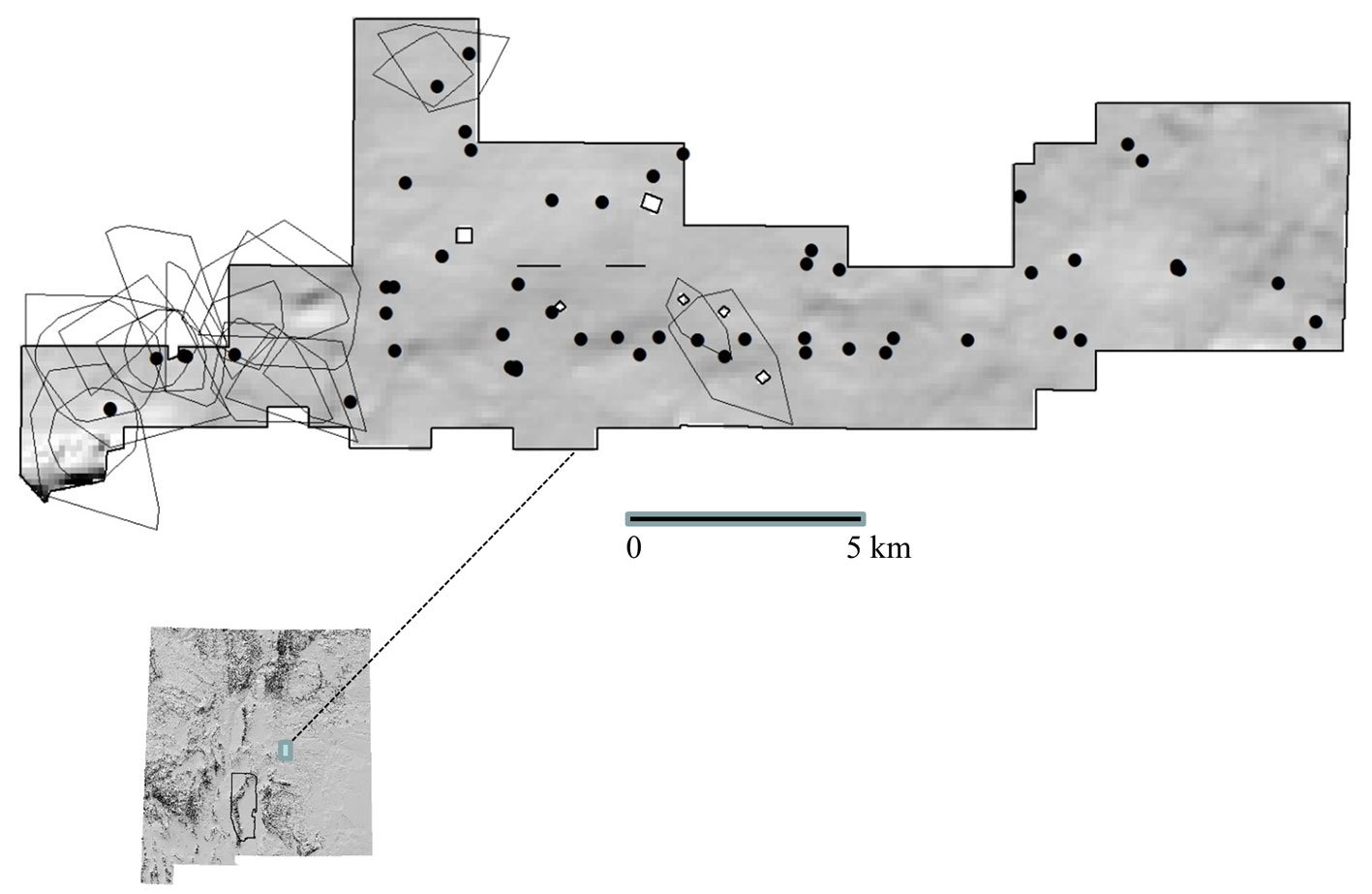
Figure 1. Area of study: Tláloc and Telapon are in the Sierra Nevada and Nevado de Toluca (both in green color). Present protected areas in Sierra Nevada (Izta-Popo-Zoquiapan National Park) and Nevado de Toluca (both are delineated by dashed lines). The new volcano rabbit distribution area in Tláloc and Telapon is not fully embraced by the Protected Area in Izta-Popo National Park. Map by Luis Antonio García Almaraz.
On the Tláloc, the presence of R. diazi was recorded in 67 of the 634 sites (Fig. 3). Most were on the southwest slope, which covers 1,537 ha of the volcano rabbit habitat in the sampled area. According to the latrine number per surface, the abundance of R. diazi on Tláloc was 0.047 latrines / m2. The elevational distribution ranges between 3,400 and 3,900 m asl, with a higher abundance between 3,700 and 3,800 m asl (p < 0.05, 95% confidence) (Table 2), as well as in sites with evidence of recent burning (25 sampling sites) and reforestation (12 sampling sites).
Table 2
Contrasts between Kaiser-Meyer-Olkin suitability measurement and Bartlett´s sphericity test. Both measurements are consistent with the 3,700-3,800 elevation range as the most suitable one for the presence of the volcano rabbit on Tláloc.
Kaiser-Meyer-Olkin suitability measurement
00.626
Bartlett´s sphericity test
Chi-squared
948.054
Degrees of freedom
78
Level of significance
p < 0.01
There was significant variation in the frequency of volcano rabbit latrine among habitats (Fig. 4). The pine forest-bunchgrass land (10% of the total area) and the alder forest (0.16% of the total area) habitats had higher frequency values than expected.
The Principal Component Analysis was the relationships between variables and the influence on each component (Fig. 5). According to this, fire and reforestation variables were positively correlated with each other. This means that the presence of any of these variables in the highland pine forest and the forest bunchgrass land habitat increases the probability of finding R. diazi.
Discussion
Our results demonstrate that ecological conditions are not the only driving factor to explain the present distribution pattern of the volcano rabbit. Here it is documented that the Tláloc and Nevado de Toluca volcanoes share similar ecological characteristics. They also share these with those reported in the Sierra Chichinautzin, Iztaccíhuatl, and Popocatépetl volcanoes. These are places where the volcano rabbit’s presence has been proven indisputably (Velázquez & Guerrero, 2019). In Figure 2, we documented the structural and species composition similarities among habitats on Tláloc and Nevado de Toluca. Velázquez and Heil (1996), as well as Hunter and Cresswell (2015), strongly state that ecological factors were key drivers of the presence of the volcano rabbit. The intensive sampling conducted in this study (as shown in Figure 3) leaves no doubt that high-elevation habitats from these 2 volcanoes are alike ecologically.
The presence of the volcano rabbit on Nevado de Toluca was reported by local farmers. The most academically outstanding evidence of this was given by González et al. (2014) in 1998. However, we assume that this evidence was either erroneous or derived from an introductory exercise that was done in at least 2 attempts (pers. com.), therefore, there were never native populations of R. diazi on Nevado de Toluca. No trace of the current presence of the volcano rabbit was found on Nevado de Toluca despite all the ecological affinities. This result supports the contribution of Hoth et al. (1987) and, more recently, of Murga-Cortés et al. (2020) and Monroy-Vilchis et al. (2020), who conducted photo-trapping and reached the same conclusion.
Figure 2. Ordination diagrams showing habitat affinities among the study areas. The triangle symbols represent plant species, whereas arrows indicate variable locations within the ordination diagram. The top diagram (denoted as A) shows the Tláloc Volcano where the 4 plant communities depicted by their dominant species (here listed) occurred. The bottom diagram (denoted as B) shows the Nevado de Toluca Volcano where 3 out of the 4 plant communities depicted by their dominant species (here listed) occurred. (A) The Tláloc Volcano: 1, pine forest-bunchgrass land: Pinus hartwegii-Senecio cinerarioides-Festuca- Barkleyanthus salicifolius-Lupinus montanus- Agrostis-Calamagrostis. 2, Alder forest: Alnus jorullensis-Roldana platanifolia-Pinus pseudostrobus-Senecio-Salix cana-Acaena elongata-Gnaphalium-Ageratina pazcuarensis-Castilleja pectinata-Trisetum-Abies religiose. 3, Cypress forest: Cupressus lusitanica-Arbutus xalapensis-Cirsium jorullense-Ribes ciliatum-Quercus laurina-Symphoricarpos microphyllus-Rumex acetosella-Ribes microphyllum-Baccharis conferta. 4, Other habitats: Juniperus monticola-Robinsonecio gerberifolius, Cirsium nivale-Roldana angulifolia-Alchemilla procumbens-Senecio toluccanus. Axis eigenvalues l: 1: 0.368, 2: 0.065, 3: 0.044 and 4: 0.035. (B) The Nevado de Toluca Volcano: 1, pine forest-bunchgrass land: Pinus hartwegii-Senecio cinerarioides-Festuca-Barkleyanthus salicifolius-Lupinus montanus-Agrostis-Calamagrostis-Eryngium proteaflorum-Penstemon gentianoides-Senecio tolucanus-Ribes microphyllum-Muhlenbergia. 2, Alder forest: Alnus jorullensis-Roldana platanifolia-Pinus patula-Senecio-Acaena elongata-Castilleja toluccensis- Symphoricarpos microphyllus-Baccharis conferta-Roldana angulifolia-Stipa-Quercus laurina-Trisetum-Abies religiosa. 3, Other habitats: Salix cana-Cupressus lusitanica, Pinus montezumae-Arbutus xalapensis-Buddleja cordata. Axis eigenvalues l: 1: 0.182, 2: 0.060, 3: 0.023 and 4: 0.015.
Figure 3. Abundance and distribution of Romerolagus diazi on Tláloc Volcano (1,537 ha). Colors contrast different vegetation types and areas comprising different volcano rabbit abundances. Low: 0.0026-0.0279 l/m2; medium: 0.0280-0.0532 l/m2; high: 0.0533-0.1921 l/m2. Sampling sites surveyed are denoted by white spots. Map by Luis Antonio García Almaraz.
Our findings let us infer that geological and biogeographical attributes play a role in explaining the absence of the volcano rabbit on Nevado de Toluca. The Tláloc Volcano arose 1.8 million years ago (Osuna et al., 2021) and the Nevado de Toluca arose 2.6 million years ago (García-Palomo et al., 2002). These 2 sites have gone through many volcanic events. Nonetheless, the most recent volcanic activity in the area has only been experienced in the Nevado de Toluca and the Popocatépetl (this volcano is still in a period of activity).
Figure 4. Observed and expected frequencies among habitat types in the Tláloc Volcano. Positive values represent volcano rabbit habitat preference greater than expected, while negative values represent volcano rabbit habitat preference less than expected (CC = 274.87, df = 3, p < 0.05).
Figure 5. Principal component analyses ordination diagram where 63% of the total variance was explained by 3 variables related to the presence of the volcano rabbit, namely: old burning traces, reforestation practices, and herbaceous layer.
Furthermore, recent research using ultraconserved genetic elements among lagomorphs (Cano et al., 2021) demonstrated that the volcano rabbit diversified from its ancestor during the Pliocene/Miocene transition (time scale: 5.33 Ma), while Osuna et al. (2020) estimate that it began its diversification ca. 1.4 Ma (Sierra Nevada and Sierra Chichinautzin). As stated by Montero (2002) and Siebe and Macías (2006), the Sierra Nevada and Nevado de Toluca volcanoes developed during the Pleistocene (time scale: 2.5 ~ 0.1 Ma). During the Late Pleistocene and the Upper Holocene (around 0.01 million years ago), many drastic climatic changes took place. These changes impacted species distribution patterns.
Based upon the present results and those of Cano et al. (2021), we postulate that the populations of R. diazi found refuges in high volcanoes during the ice retreat of the Early Holocene. The volcano rabbit populations were partially depleted on Popocatépetl and totally depleted on Nevado de Toluca because of recurrent eruptions during the transition from the Late Pleistocene to the Upper Holocene (Siebe & Macías, 2006). This is without discarding the urban expansion and overgrazing that occurs in the Nevado de Toluca, as there are human settlements up to 3,500 m asl; human disturbance of habitats advances from the bottom up, reducing and isolating them more. Some of the consequences that can come with rising temperature, as well as changes in precipitation, are the extinction of species and the decline of their populations (Domínguez-Pérez, 2007); areas potentially habitable by the zacatuche tend to be confined to the higher elevation zones.
Romerolagus survives from the late Pleistocene, as its presence was recorded from a tooth belonging to a zacatuche in Valsequillo, Puebla (Cruz-Muñoz et al., 2009), although it remained at the Iztaccíhuatl and Tláloc volcanoes of Sierra Nevada during the Late Holocene. The ecological effects of climate change during the Pleistocene led to the loss or fragmentation of habitats (Koch & Barnosky, 2006), which probably completely extinguished the habitable areas for R. diazi in Valsequillo. Later, during the Northgrippian and Meghalayan Holocene periods, it expanded its present distribution to the Sierra Chichinautzin. This hypothesis is coherent with the theory of island biogeography (MacArthur & Wilson, 1967), which is based on the principle that large, connected islands support greater resilience compared to small, isolated islands. This hypothesis is similar to Luna-Vega (2018), who sustained that Central Mexico has been subject to paleoclimatic, tectonic, and glacier advance and retreat events that have caused contraction, isolation, differentiation, speciation, and range expansion of local species. The Popocatépetl and Iztaccíhuatl volcanoes function as biogeographic islands in the midst of warmer climates and diverse types of vegetation, limiting the migration of the zacatuche. In addition, the Pleistocene-Holocene boundary extinction of megafauna was important in reducing predation or vegetation change associated with the loss of disperser species as it altered the distribution of smaller species such as the zacatuche (Ferrusquía-Villafranca et al., 2010).
The present distribution range of the volcano rabbit includes the Tláloc Volcano in the Sierra Nevada and excludes Nevado de Toluca. Although Tláloc is adjacent to Iztaccíhuatl, one of the larger and potentially better-protected areas of habitat (Hunter & Cresswell, 2015), 35 years ago, periodic visits were made in this area without finding evidence of the volcano rabbit (Hoth et al., 1987). Based on the above, it is possible to deduce that disturbances such as geological events and human activities have occurred in the same way the habitats of the entire range of distribution and the populations only translocate but regionally remain, namely, the populations undergo local distributional shifts but rarely go extinct from an entire region. Geological events, biogeographical processes, ecological conditions, and human activities are all connected to explain the present distribution pattern of this endemic and endangered species. Our results are expected to have positive implications for conservation in the Izta-Popo National Park and especially for the zacatuche populations on Tláloc.
Currently, Romerolagus diazi conservation on the Tláloc Volcano in Sierra Nevada is mainly the result of local actors who have engaged in managing their land favoring the conservation of this emblematic species. Ongoing research on the potential for participatory landscape conservation to engage local actors as allies in conservation tasks is still to be documented (sensu Velázquez et al., 2003). Further research to document if these connected driving forces also explain the distribution of species that are sympatric with the volcano rabbit is yet to be conducted.
Acknowledgments
We would like to acknowledge the local landowners (ejidatarios) for their support and to the Conanp for their approval. Special thanks go to the High Mountain Group students who assisted us with fieldwork. This study was funded by the project Conacyt-Conafor/A3-S-130105, and by the Universidad Nacional Autónoma de México (Dirección General de Asuntos del Personal Académico-UNAM IN105721).
References
Anderson, B., Akçakaya, H., Araújo, M., Fordham, D., Martinez, M., Thuiller, W., & Brook, B. (2009). Dynamics of range margins for metapopulations under climate change. Proceedings of the Royal Society B: Biological Sciences, 276, 1415–1420. https://doi.org/10.1098/rspb.2008.1681
Arce, J. L., Macías, J. L., & Vázquez-Selem, L. (2003). The 10.5 ka Plinian eruption of Nevado de Toluca Volcano, Mexico: Stratigraphy and hazard implications. GSA Bulletin, 115, 230–248. https://doi.org/10.1130/0016-7606(2003)115%3C0230:TKPEON%3E2.0.CO;2
Astudillo-Sanchez, C., Villanueva-Díaz, J., Endara Agramont, A., Nava Bernal, G., & Gómez Albores, M. (2017). Influencia climática en el reclutamiento de Pinus hartwegii Lindl. del ecotono bosque-pastizal alpino en Monte Tláloc, México. Agrociencia, 51, 105–118. https://doi.org/10.35196/rfm.2024.2.209
Bartlett, M. S. (1950). Tests of significance in factor analysis. British Journal of Mathematical and Statistical Psychology, 3, 77–85. https://doi.org/10.1111/j.2044-8317.1950.tb00285.x
BOLFOR, Mostacedo, B., & Fredericksen, T. S. (2000). Manual de métodos básicos de muestreo y análisis en ecología vegetal. Santa Cruz de la Sierra, Bolivia: Editora El País.
Cano-Sánchez, E., Rodríguez-Gómez, F., Ruedas, L.A., Oyama, K., León-Paniagua, L., Mastretta-Yanes, A., & Velázquez, A. (2022). Using ultraconserved elements to unravel lagomorph phylogenetic relationships. Journal of Mammalian Evolution, 29, 395–411. https://doi.org/10.1007/s10914-021-09595-0
Childs, C. (2004). Interpolating surfaces in ArcGIS spatial analyst. ArcUser, July-September, 3235, 32–35.
Cruz-Muñoz, V., Arroyo-Cabrales, J., & Graham, R. W. (2009). Rodents and lagomorphs (Mammalia) from the late-Pleistocene deposits at Valsequillo, Puebla, México. Current Research in the Pleistocene, 26, 147–149.
Dauber, E. (1995). Guía práctica y teórica para el diseño de un inventario forestal de reconocimiento. Santa Cruz de la Sierra: BOLFOR.
Domínguez-Pérez, A. (2007). Efecto del cambio climático en la distribución del conejo endémico de México Romerolagus diazi (Lagomorpha: Leporidae) (Tesis). Ciudad de México: Universidad Nacional Autónoma de México.
Espinasa-Pereña, R., & Martín-Del Pozzo, A. (2006). Morphostratigraphic evolution of Popocatépetl volcano, México, Neogene-Quaternary continental margin volcanism: a perspective from México. Special Paper. Geological Society of America, 402, 101–123. https://doi.org/10.1130/2006.2402%2805%29
Esri Inc (Environmental Systems Research Institute). (2019). ArcMap 10.8. Redlands, CA: Esri Inc. Software.
Etherington, T. R. (2020). Discrete natural neighbour interpolation with uncertainty using cross-validation error-distance fields. Computer Science – PeerJ, 6, e282. https://doi.org/10.7717/peerj-cs.282
Fa, J. E., Romero, F. J., & López, P. (1992). Habitat use by parapatric rabbits in a Mexican high-altitude grassland system. Journal of Applied Ecology, 29, 357–370. https://doi.org/10.2307/2404505
Ferrusquía-Villafranca, I., Arroyo-Cabrales, J., Martínez-Hernández, E., Gama-Castro, J., Ruiz-González, J., Polaco, O. J. et al. (2010). Pleistocene mammals of Mexico: a critical review of regional chronofaunas, climate change response and biogeographic provinciality. Quaternary International, 217, 53–104. https://doi.org/10.1016/j.quaint.2009.11.036
García, F., Campos, M., Guerrero, E., Rizo, A., Brito, G., & Farías, G. (2018). Manual de monitoreo del conejo de los volcanes (Romerolagus diazi): procedimiento para estimar la densidad absoluta mediante conteo de excretas en transectos con parcelas. Ciudad de México: DGCORENA/ DGZVS/ SDS/ CEPANAF, UNAM/ UAEM.
García, R. J., & Di Marco, M. (2020). Drivers and trends in the extinction risk of New Zealand’s endemic birds. Biological Conservation, 249, 108730. https://doi.org/10.1016/j.biocon.2020.108730
García-Palomo, A., Macías, J. L., Arce, J. L., Capra, L., Garduño, V. H., & Espíndola, J. M. (2015). Geology of the Nevado de Toluca Volcano and surrounding areas, Central Mexico. Boulder, Colorado: Geological Society of America.
González, G. J., Rosas, B. V., & Pulido, J. R. (2014). A recent record of the volcano rabbitt (Romerolagus diazi) from the Nevado de Toluca, State of Mexico. Revista Mexicana de Mastozoología (Nueva época), 3, 149–150. https://doi.org/10.22201/ie.20074484e.1998.3.1.89
Hoth, J., Velázquez, A., Romero, F., Leon, L., Aranda, M., & Bell, D. (1987). The volcano rabbit: a shrinking distribution and a threatened habitat. Oryx, 21, 85–91. https://doi.org/10.1017/S0030605300026600
Hunter, H., & Cresswell, W. (2015). Factors affecting the distribution and abundance of the endangered volcano rabbit Romerolagus diazi on the Iztaccíhuatl volcano, Mexico. Oryx, 49, 366–375. https://doi.org/10.1017/S0030605313000525
IBM Corp. (2019). IBM SPSS Statistics for Windows, Version 26.0. Armonk, NY: IBM Corp.
Kaiser, H. F. (1974). An index of factorial simplicity. Psychometrika, 39, 31–36. https://doi.org/10.1007/BF02291575
Koch, P. L., & Barnosky, A. D. (2006). Late Quaternary extinctions: state of the debate. Annual review of ecology, evolution, and systematics,37, 215–250. https://doi.org/10.1146/annurev.ecolsys.34.011802.132415
López, P., Romero, J., & Velázquez, A. (1996). Las actividades humanas y su impacto en el hábitat del conejo conejo de los volcanes. In A. Velázquez, F. J. Romero & P. López (Eds.), Ecología y conservación del conejo de los volcanes y su hábitat (pp 119–131). México D.F.: Fondo de Cultura Económica.
Luna-Vega, I. (2018). Aplicaciones de la biogeografía histórica a la distribución de las plantas mexicanas. Revista Mexicana de Biodiversidad, 79, 217–241. https://doi.org/10.22201/ib.20078706e.2008.001.523
MacArthur, R. H., & Wilson, E. O. (1967). The Theory of Island Biogeography. Princeton, NJ.: Princeton University Press.
Mayer, H., & Ott, E. (1991). Silviculture in mountain forest-management of protection forest: a silvicultural contribution to landscape ecology and environmental protection, 2nd Ed. Stuttgart, Germany: Gustav Fischer.
Monroy-Vilchis, O., Luna-Gil, A. A., Endara-Agramont, A. R., Zarco-González, M. M., & González-Desales, G. (2020). Nevado de Toluca: habitat for Romerolagus diazi?Animal Biodiversity and Conservation, 43, 115–121. http://dx.doi.org/10.32800/abc.2020.43.0115
Monroy-Vilchis, O., & Velázquez, A. (2002). Distribución regional y abundancia del lince (Lynx rufus escuinape) y el coyote (Canis latrans cagottis) por medio de estaciones olfativas: un enfoque espacial. Ciencia Ergo Sum, 9, 293–300.
Montero, I. A. (2002). Atlas arqueológico de la Alta Montaña Mexicana. Ciudad de México: Semarnat-Conafor.
Murga-Cortés, A., Brito-González, D., Dirzo-Uribe, G., González-Zariñana, B., Rizo-Aguilar, A., & Guerrero, J. A. (2020). Use of mitochondrial DNA from feces to evaluate the range of secretive species: the case of volcano rabbit. Therya Notes, 1, 50–53. http://dx.doi.org/10.12933/therya_notes-20-12
Osuna, F., González, D., de los Monteros, A. E., & Guerrero, J. A. (2020). Phylogeography of the volcano rabbit (Romerolagus diazi): the evolutionary history of a mountain specialist molded by the climatic volcanism interaction in the Central Mexican highlands. Journal of Mammalian Evolution, 27, 745–757. https://doi.org/10.1007/s10914-019-09493-6
Osuna, F., Guevara, R., Martínez-Meyer, E., Alcalá, R., & de los Monteros, A. E. (2021). Factors affecting presence and relative abundance of the endangered volcano rabbit Romerolagus diazi, a habitat specialist. Oryx, 1–10. https://doi.org/10.1017/S0030605320000368
Ottaviani, G., Keppel, G., Götzenberger, L., Harrison, S., Opedal, Ø. H, Conti, L. et al. (2020). Linking plant functional ecology to island biogeography. Trends in Plant Science, 25, 329–339. https://doi.org/10.1016/j.tplants.2019.12.022
Rizo-Aguilar, A., Guerrero, J., Mihart, M., & Romero, A. (2015). Relationship between the abundance of the endangered volcano rabbit (Romerolagus diazi) and vegetation structure in the Sierra Chichinautzin Mountain range, Mexico. Oryx, 49, 360–365. https://doi.org/10.1017/S0030605315000782
Sibson, R. (1981). A brief description of natural neighbor interpolation. In W. John Sons (Eds.). Interpolating multivariate data (pp 21–36). Nueva York: John Wiley & Sons.
Siebe, C., & Macías, J. L. (2006). Volcanic hazards in the Mexico City metropolitan area from eruptions at Popocatépetl, Nevado de Toluca, and Jocotitlán stratovolcanoes and monogenetic scoria cones in the Sierra Chichinautzin Volcanic Field. Special paper. Geological Society of America, 402, 253–277. http://dx.doi.org/10.1130/2004.VHITMC.SP402
Smith, Y. C. E, Smith, D. A. E, Ramesh, T., & Downs, C. T. (2020). Landscape-scale drivers of mammalian species richness and functional diversity in forest patches within a mixed land-use mosaic. Ecological Indicators, 113, 106176. https://doi.org/10.1016/j.ecolind.2020.106176
ter Braak, C. J. F. (2002). CANOCO. Version 4.5. Plant Research International, Wageningen University and Research Centre, Wageningen, The Netherlands.
Uriostegui-Velarde, J. M., González-Romero, A., Pineda, E., Reyna-Hurtado, R., Rizo-Aguilar, A., & Guerrero, J. A. (2018). Configuration of the volcano rabbit (Romerolagus diazi) landscape in the Ajusco-Chichinautzin Mountain Range. Journal of Mammalogy, 99, 263–272. https://doi.org/10.1093/jmammal/gyx174
Velázquez, A., & Guerrero, J. A. (2019) Romerolagus diazi. The IUCN Red List of Threatened Species 2019: e.T19742A45180356.
Velázquez, A. (1993). Man-made and ecological habitat fragmentation: study case of the volcano rabbit (Romerolagus diazi). Zeitschrift fur Saugetierkunde, 58, 54–54.
Velázquez, A. (1994). Distribution and population size of Romerolagus diazi on El Pelado Volcano, México. Journal of Mammalogy, 75, 743–749. https://doi.org/10.2307/1382525
Velázquez, A., Gerardo, B., Romero, F. J., & Pérez, V. A. (2003). A landscape perspective on biodiversity conservation: the case of Central Mexico. Mountain Research and Development, 23, 240–246. https://doi.org/10.1659/0276-4741(2003)023[0240:ALPOBC]2.0.CO;2
Velázquez, A., & Heil, G. W. (1996). Habitat suitability study for the conservation of the volcano rabbit (Romerolagus diazi). Journal of Applied Ecology, 33, 543–554. https://doi.org/10.2307/2404983
Velázquez, A., Larrazábal, A., & Romero, F. J. (2011). Del conocimiento específico a la conservación de todos los niveles de organización biológica. El caso del conejo de los volcanes y los paisajes que denotan su hábitat. Investigación Ambiental, 3, 59–62.
Weber, G., Arce, J. L., Ulianov, A., & Caricchi, L. (2019). A recurrent magmatic pattern on observable timescales prior to plinian eruptions from Nevado de Toluca (Mexico). Journal of Geophysical Research: Solid Earth, 124, 10999–11021. https://doi.org/10.1029/2019JB017640
Miguel Ángel Mosqueda-Cabrera *, Diana Laura Desentis-Pérez y Tania Araceli Padilla-Bejarano
a Centro de Investigación Científica y de Educación Superior de Ensenada, Departamento de Biología de la Conservación, Carretera Tijuana-Ensenada # 3918, Zona Playitas, 22860 Ensenada, Baja California, Mexico
b Universidad Autónoma de Baja California, Facultad de Ciencias, Carretera Transpeninsular # 3917, Colonia Playitas, 22860 Ensenada, Baja California, Mexico
Received: 28 February 2024; accepted: 01 July 2024
Resumen
Las larvas de tercer estadio avanzado (AdvL3) de Gnathostoma sp. I aisladas de la musculatura de Dormitator latifrons y Rhamdia guatemalensis son morfológica y molecularmente iguales entre sí y se relacionan genéticamente con un juvenil aislado del hígado de Didelphis marsupialis, en la cuenca del río Ostuta, Oaxaca. Asimismo, son diferentes de las 3 especies de Gnathostoma descritas para México por el tamaño del cuerpo, por los ganchos del bulbo cefálico en la fase AdvL3 y por la presencia de un prepucio cuticular en el extremo posterior de un macho juvenil. A través del marcador molecular COI, un análisis de distancias genéticas y la inferencia de la filogenia entre las especies del género, se concluye que Gnathostoma sp. I está estrechamente emparentada, pero taxonómicamente es diferente a G. turgidum y a las otras especies presentes en México y el mundo, aun cuando falta material para establecerla como especie nueva. Por otro lado, con base en características morfológicas se documenta el hallazgo de las AdvL3 de G. lamothei (en Rhambdia guatemalensis y Lontra longicaudis) y la AdvL3 de otra especie no identificada (en R. guatemalensis y Synbranchus marmoratus), pero distinta a las anteriores de acuerdo con evidencias morfológicas y moleculares.
Palabras clave: Gnathostoma spp.; Tercer estadio avanzado; Filogenia; México; Marsupiales
The high morphological variation found in the immature stages of the nematode Gnathostoma sp. I is not supported by molecular information
Abstract
The third-stage advanced larvae (AdvL3) of Gnathostoma sp. I isolated from the musculature of Dormitator latifrons and Rhamdia guatemalensis are identical to each other morphological and molecularly, and are genetically related to a juvenile isolated from the liver of Didelphis marsupialis, in the Ostuta River basin, Oaxaca. They are different from the 3 species of Gnathostoma described from Mexico by body size and the hooks of the cephalic bulb in the AdvL3 stage, as well as, in the presence of a cuticular pouch at the posterior end of the juvenile male. Through the COI molecular marker, a genetic distance analysis, and phylogenetic inference among the species of the genus, we conclude that Gnathostoma sp. I is closely related to, but distinct from G. turgidum and from other species found in Mexico and worldwide, even though there is not enough material to establish it as a new species. Additionally, based on morphologic characteristics, we documented the discovery of AdvL3 of G. lamothei (in Rhambdia guatemalensis and Lontra longicaudis) and AdvL3 of another unidentified species (in R. guatemalensis and Synbranchus marmoratus), which is distinct to above according to morphologic and molecular evidence.
Keywords: Gnathostoma spp.; Advanced third stage; Phylogeny; Mexico; Marsupials
Introducción
Entre el enorme conjunto de especies de helmintos que se distribuyen en México se encuentra el género Gnathostoma Owen, 1836(Spirurida: Gnathostomatidae) conformado por 12 especies válidas (Almeyda-Artigas, 1991; Bertoni-Ruiz et al., 2005; Miyazaki, 1954). Tres de ellas se distribuyen en México: Gnathostoma binucleatum Almeyda-Artigas, 1991; Gnathostoma turgidum Stossich, 1902 y Gnathostoma lamothei Bertoni-Ruiz, García-Prieto, Osorio-Sarabia y León-Règagnon, 2005 (Gaspar-Navarro et al., 2013). Las especies presentan una alta especificidad hacia mamíferos carnívoros como sus hospederos definitivos; G. binucleatum (Canidae, Felidae, Suidae), G. lamothei (Procyonidae) y G. turgidum (Didelphidae) (Pérez-Álvarez et al., 2008). El hospedero definitivo adquiere la infección al alimentarse de los segundos hospederos intermediarios, peces dulceacuícolas para las 2 primeras especies (Almeyda-Artigas, 1991; Bertoni-Ruiz et al., 2005), ranas y accidentalmente peces para la última (Mosqueda-Cabrera et al., 2009, 2023).
El objetivo de la presente investigación fue describir un morfotipo de Gnathostoma que difiere morfológicamente de las especies conocidas para didélfidos de México, proveniente de una zona no explorada previamente, la cuenca del río Ostuta, Oaxaca.
Materiales y métodos
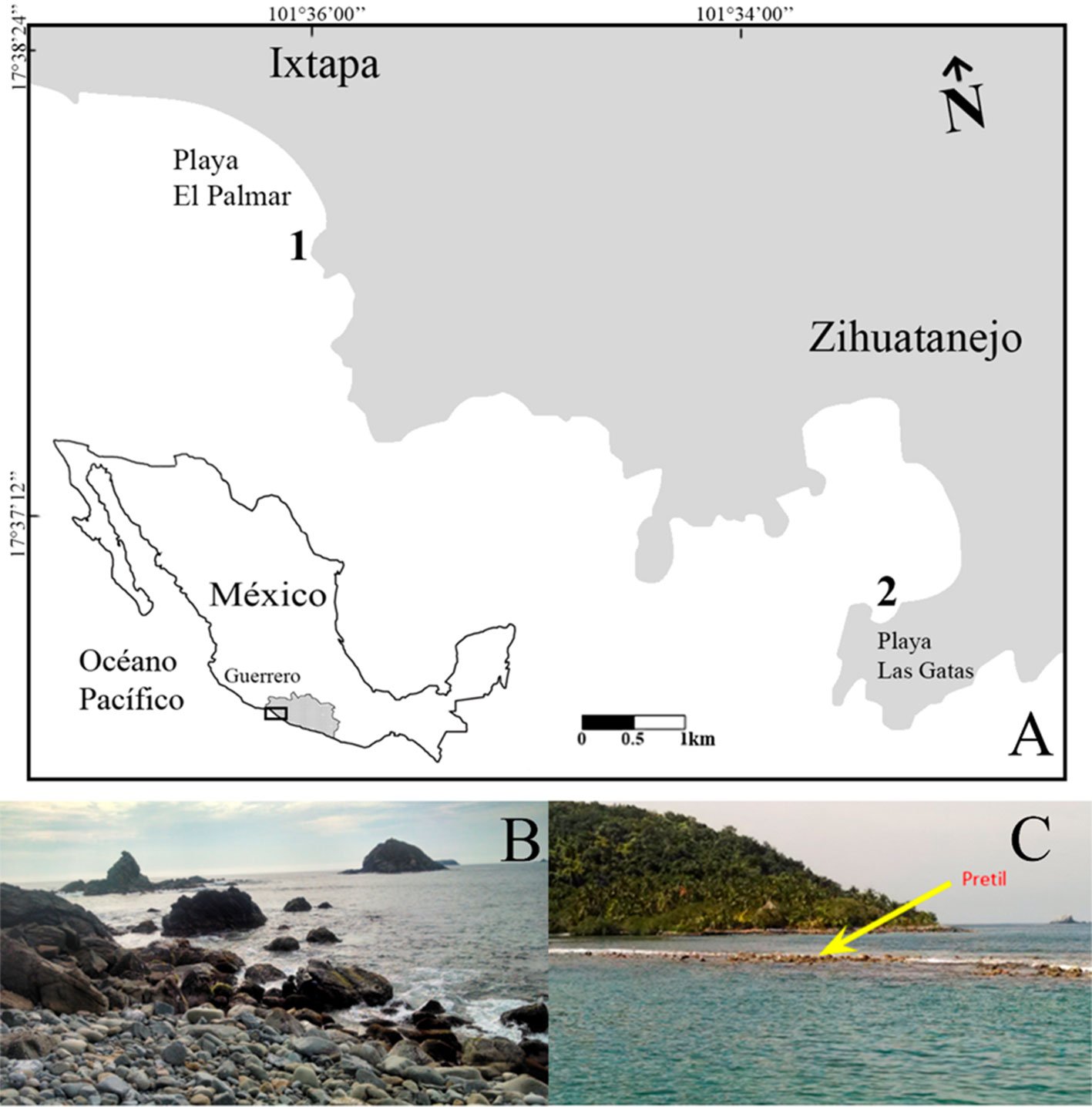
La cuenca del río Ostuta forma parte de la porción oriente de la región hidrográfica Tehuantepec (RH22). Se localiza en la zona suroriente del estado de Oaxaca, que limita con Chiapas. La laguna Las Garzas (16°17’46” N, 94°27’17” O), es un cuerpo de agua semipermanente, remanente de un antiguo cauce de río ubicado en la región hidrográfica Costa de Chiapas (RH23) en la cuenca del mar Muerto, que colinda al oeste con la cuenca del río Ostuta (Conagua, 2021) y es irrigada por la misma durante lluvias torrenciales (fig. 1).
Esta investigación fue conducida debido al hallazgo fortuito de larvas tercer estadio avanzado (AdvL3) en las heces de la nutria neotropical Lontra longicaudis de la cuenca del río Ostuta, Oaxaca durante abril y mayo de 2018. Posteriormente, durante el 2022 se realizó la búsqueda de larvas de Gnathostoma en peces de este río y en cuerpos de agua asociados a la región hidrográfica (RH23). Para su captura se utilizaron redes de pesca como atarrayas y chinchorros. La musculatura de los peces fue revisada a contraluz entre 2 vidrios y posteriormente digerida con pepsina artificial (16 gr de pepsina, 6 gr de NaCl y 8 ml de HCl en 1 L de agua). La búsqueda de las larvas se realizó con ayuda de un microscopio estereoscópico; fueron fijadas en alcohol etílico al 70% caliente y conservadas en alcohol etílico al 70% frío. Para su estudio fueron transparentadas con lactofenol de Amman y observadas bajo el microscopio compuesto. Todas las medidas se presentan en micras, se especifica el rango y entre paréntesis el promedio seguido de la desviación estándar y el número de observaciones. Los parámetros de la infección fueron calculados de acuerdo con Bush et al. (1997). Se tomaron fotografías con una cámara digital montada a un microscopio óptico y los dibujos fueron realizados con ayuda una cámara clara. La captura y el sacrificio del tlacuache común Didelphis marsupialis fue realizada de acuerdo con Almeyda-Artigas et al. (2010) e identificado por la morfología craneal siguiendo a Gardner (1973). El material de referencia fue depositado en la Colección Nacional de Helmintos (CNHE) del Instituto de Biología, Universidad Nacional Autónoma de México (IB-UNAM). La obtención de los organismos se realizó bajo el permiso de colecta SCPA/DGVS/03184/22 expedido por la Secretaría de Medio Ambiente y Recursos Naturales, México.
Figura 1. Cuenca del río Ostuta, Oaxaca en la región hidrográfica Tehuantepec (RH22). Laguna Las Garzas en la región hidrográfica Costa de Chiapas (RH23). Mapa elaborado por D.L. Desentis Pérez.
La extracción del DNA se llevó a cabo utilizando el kit de extracción DNeasy Blood & Tissue (QIAGEN). Se amplificó la región del segundo espaciador interno transcrito (ITS2) y la subunidad I del citocromo c oxidasa (COI) mediante la reacción en cadena de la polimerasa (PCR por sus siglas en inglés). La amplificación de las secuencias nucleotídicas parciales de los genes mencionados se llevó a cabo a partir de reacciones compuestas por una solución de 8.5 µl de H2O, 3 µl de buffer 5x, 0.2 µl de cada oligonucleótido, 0.1 µl de enzima Taq polimerasa (Bioline) y 3 µl de DNA genómico en un volumen total de 15 µl. La región ITS2 se amplificó con los oligonucleótidos NEWS2 (forward) 5ʼ-TGTGTCGATGAAGAACGCAG-3ʼ e ITS2-RIXO (reverse) 5ʼ-TTCTATGCTTAAATTCAGGGG-3ʼ (Almeyda-Artigas et al., 2000a), con el siguiente perfil térmico: 1 ciclo de 94 °C por 1 min; 5 ciclos de 92 °C por 30 s, 45 °C por 30 s y 72 °C por 1 min; 35 ciclos de 92 °C por 30 s, 53 °C por 30 s y 72 °C por 1 min; elongación final a 72 °C por 4 min. Las secuencias parciales del gen mitocondrial COI se amplificaron con los cocteles de oligonucleótidos previamente preparados según Prosser et al. (2013), utilizando los siguientes oligonucleótidos: NemF1_t15ʼCRACWGTWAATCAYAARAATATTGG3-ʼ, NemF2_t1 5ʼ-ARAGATCTAATCAT AAAGATATYGG3-ʼ, NemF3_t1 5ʼ-ARAGTTCTAATCATAARGATATTGG-3ʼ (forward) y NemR1_t1 5ʼ-AAACTTCWGGRTGACCAAAAAATCA-3ʼ, NemR2_t1 5ʼ-AWACYTCWGGRTGMCCAAAAAAYCA-3ʼ, NemR3_t1 5ʼAAACCTCWGGATGACCAAAAAATCA-3ʼ (reverse) implementando el siguiente perfil térmico: 1 ciclo de 94 °C por 1 min; 5 ciclos de 94 °C por 40 s, 45 °C por 40 s y 72 °C por 1 min; 35 ciclos de 94 °C por 40 s, 53 °C por 40 s y 72 °C por 1 min; elongación final a 72 °C por 5 min. Los productos de la PCR fueron purificados mediante el kit de purificación QUIAquick PCR (50) (QIAGEN). Las secuencias fueron obtenidas mediante el secuenciador de DNA automatizado ABI Prism 310 en el Laboratorio de Secuenciación Genómica del PABIO-UNAM. En el caso del ITS-2 se usaron los oligonucleótidos: NEWS2 e ITS2-RIXO para la secuenciación, en el caso del COI se usaron los oligonucleótidos M13F (5ʼ-TGTAAAACGACGGCCAGT-3ʼ) y M13R (5ʼ-CAGGAAACAGCTATGAC-3ʼ) (Messing, 1993).
Las secuencias obtenidas se alinearon en el programa MAFFT V7 (en línea) con sus homólogas (COI/ITS2) disponibles en el repositorio GenBank del NCBI (National Center for Biotechnology Information), correspondientes a especies nominales del género Gnathostoma en México y una especie del género Anisakis (A. pegreffi FJ907317/AY603531) como grupo externo: G. binucleatum (AB180103/EU915244), G. lamothei (KF648543), G. turgidum (KT894798/KF648548), G. spinigerum (AB037132/KF648553), G. nipponicum (JQ824059/JN408314), G. hispidum (JQ824056/JQ824057). A partir de los alineamientos múltiples de secuencias se realizó un análisis de distancias genéticas en el programa MEGA X 11.0.13 para establecer la similitud entre las distintas especies utilizando el modelo Kimura 2 parámetros (K2P) de acuerdo con Hebert et al. (2003). El análisis filogenético se realizó con los 2 marcadores moleculares (COI, ITS-2), de manera independiente y posteriormente fueron concatenados con un ajuste manual en el programa Mesquite v. 3.6 (Maddison y Maddison, 2019). La inferencia filogenética se realizó utilizando el criterio de inferencia bayesiana (IB) en el programa MrBayes v. 3.2.1 (Ronquist et al., 2012). Los resultados se ilustraron en un árbol filogenético construido en el programa FigTree v. 1.4.2 (Rambaut, 2006).
Descripción
Gnathostoma sp. I (figs. 2-4)
Juvenil. Bulbo cefálico con ganchos de una sola punta dispuestos en 10 hileras completas, mide 393.6 × 861, de largo y ancho, respectivamente. Dos papilas cervicales laterales, derecha e izquierda, ambas en la décima hilera. Ancho del cuerpo a la altura de la intersección esófago-intestino 1,479.60. Esófago de 14,586.39 de largo × 836.10 de ancho, cubre 58.3% respecto al ancho del cuerpo. Cuatro sacos cervicales se proyectan desde la base del bulbo cefálico, en promedio miden 2,379.69 de largo, 16.31% respecto al largo del esófago. Bursa con pequeñas espinas ventrales en sentido posteroanterior, presenta 4 pares de papilas pedunculadas; 2 pares preanales, un par adanal y 2 pares postanales; además, 4 pares de papilas no pedunculadas; un par preanal, 2 pares adanales y un par postanal. Dos espículas, la derecha 3,267.43 de largo × 142.68 de ancho; la izquierda 949.41 largo × 93.48 de ancho; proporción de 1:3.4; el extremo posterior con cutícula holgada más larga que el cuerpo, similar a un prepucio.
Espinas corporales presentes solo en la región anterior del cuerpo con variaciones en el número de puntas según la región; a, inmediatamente posteriores al bulbo cefálico, con 5-7 puntas son comunes las de 5, más largas (49.06) que anchas (22.08); b, en la región que ocupan las papilas cervicales, de 5-9 puntas son comunes las de 7 y 8, con 61.32 de largo y 31.89 de ancho; c, a la altura de los sacos cervicales, con 5 a 10, más largas (108.24) que anchas (75.80), con una a 3 puntas laterales y tronco central con 3 y 5 puntas; d, a la altura de la intersección esófago-intestino, espinas con 5 a 6 puntas más anchas que largas, 59.04 y 39.36, respectivamente, las puntas laterales generalmente más cortas y con 3 a 4 puntas centrales; e, posterior a la intersección esófago-intestino, cambian drásticamente de forma y tamaño, siendo más largas (59.04) que anchas (34.44) con un par de puntas laterales cortas y de 2 a 3 puntas centrales de igual tamaño; en la parte más posterior de la porción escamada del cuerpo se observa un gradiente donde las puntas centrales de las espinas van ensanchándose y desapareciendo las puntas laterales hasta terminar en espinas de una sola punta.
Datos morfológicos adicionales (basados en la observación directa de especímenes depositados en la CNHE 4739): macho obtenido del estómago de Didelphis marsupialis. Mide 46,000 de largo por 2,182.41 de ancho máximo. Esófago 6,625 por 542.52 de largo y ancho, respectivamente; cubre 14.4% respecto a la longitud del cuerpo. Dos papilas cervicales en 11 (izquierda) y 10 (derecha), sobre las hileras de espinas del cuerpo. Bulbo cefálico 442.80 por 939.72 de largo y ancho, respectivamente, con 9 hileras completas de ganchos con una sola punta de base gruesa y cónica. Extremo posterior con cutícula holgada corrugada y arreglo de las espinas en el cuerpo iguales a la forma juvenil que aquí se describe. Las espinas cubren 61% del cuerpo.
Resumen taxonómico
Hospedero: tlacuache común Didelphis marsupialis Linnaeus, 1758 (Didelphimorphia: Didelphidae).
Sitio de infección: hígado.
Localidad: inmediaciones del río Ostuta, San Francisco Ixhuatán, Oaxaca.
Depósito de especímenes: CNHE 12827.
Comentarios taxonómicos
Para propósitos comparativos, estudiamos especíme- nes de G. turgidum de D. marsupialis (CNHE 4739) y G. turgidum de D. virginiana (CNHE 4261, 4740, 4736). La presencia de una cutícula holgada en el extremo posterior en la forma juvenil estudiada en este trabajo y su ausencia en el adulto de G. turgidum (CNHE 4739), así como el porcentaje espinado del cuerpo (61% vs. 40%, respectivamente), son las únicas características diferentes entre las especies. La relación entre las espículas del macho, el número de puntas y arreglo de las espinas en el cuerpo no mostraron diferencias entre ambos lotes de material.
Los fragmentos de gen amplificados, ITS-2 (480 pb) y COI (702 pb), se encuentran disponibles en GenBank con números de acceso PQ149238 y PQ143178, respectivamente, y pertenecen al segundo tercio del juvenil de Gnathostoma sp. I
Figura 2. Gnathostoma sp. I parásito de D. marsupialis. a) Espícula derecha y cutícula holgada del extremo posterior; b) patrón de espinación de la bursa con papilas ventrales y laterales.
Figura 3. Extremo posterior de juvenil de Gnathostoma sp. I. (a) Cutícula holgada; b) espícula derecha y papilas de la bursa. Escala de las barras = 200 μm.
Las notables diferencias morfológicas en el tamaño del cuerpo entre las AdvL3 de Gnathostoma aisladas de los peces D. latifrons y las de G. turgidum (tabla 1), así como el tamaño de los ganchos en las 4 hileras del bulbo cefálico, nos condujeron a pensar que pudieran tratarse de especies independientes. El análisis de distancias genéticas de las secuencias (modelo K2P del ITS2) determinó que las AdvL3 obtenidas de D. latifrons y el juvenil obtenido de D. marsupialis son iguales entre sí pero también muy similares a las secuencias de G. turgidum con valores de 0.0043 para el juvenil y 0.0046 para la AdvL3. En cuanto al marcador molecular COI, en el análisis de distancias genéticas de las secuencias registramos una distancia genética de 0.0657 con respecto a las ya mencionadas y la secuencia de G. turgidum. Basados en estos datos, nuestro material podría representar una variante de G. turgidum o una especie cercanamente relacionada a ésta (fig. 5). Sin embargo, y pese a las diferencias morfológicas tan claras entre ambos taxones, preferimos adoptar una posición conservadora y no establecer a las larvas y al juvenil que recuperamos en el río Ostuta, Oaxaca, como una especie independiente hasta contar con una mayor cantidad de evidencias, tanto morfológicas (de hembras y machos adultos) como moleculares.
Figura 4. Arreglo de las espinas en el cuerpo de Gnathostoma sp. I. a) Primeras hileras del cuerpo; b) región de la papila cervical; c) región distal de los sacos cervicales; d) intersección esófago-intestino; e) región final de la superficie espinada. Escala de la barra = 100 μm.
Gnathostoma sp. I (figs. 6, 7)
Larva de tercer estadio avanzado. La siguiente descripción está basada en la observación de 23 larvas. El cuerpo mide 1,149-1,414 (1, 262 ± 90.86; 11) de largo y 94.71-129.77 (105.82 ± 12.59; 11) de ancho; está cubierto totalmente por hileras de espinas transversales, cuyo número oscila entre 180-223 (192.79 ± 11.82; 13). Bulbo cefálico 30.77-85.85 (44.69 ± 14.57; 13) de largo × 65.23-169.24 (91.90 ± 26.72; 13) de ancho; presenta espinas dispuestas en 4 hileras transversales: 27-37 (31.17 ± 2.59; 23), 28-44 (34.39 ± 3.78; 23), 30-44 (37.22 ± 3.42; 23) y 33-46 (41.26 ± 3.75; 23), de la primera a la cuarta, respectivamente. Miden: 4.44-6.22 (5.33 ± 0.68) × 1.77-2.66 (2.28 ± 0.31), 5.33-5.77 (5.64 ± 0.21) × 2.22-2.66 (2.35 ± 0.21), 5.33-6.22 (5.65 ± 0.34) × 2.66-3.55 (3.11 ± 0.26), 4.44-4.88 (4.82 ± 0.17) × 2.66-3.55 (3.11 ± 0.36), largo y ancho de la primera a la cuarta hilera, respectivamente. Cuatro sacos cervicales ocupan de 43.23 a 75.29% (58.99 ± 7.65; n = 10) de la longitud de esófago. El esófago abarca de 32 a 73.81% (40.30 ± 2.60; n = 10) del largo total y 51% de su ancho, a la altura de la intersección esófago-intestino. El poro excretor ventral, se ubica en las hileras 15-21 (18.73 ± 1.60; n = 15). Dos papilas cervicales laterales, la derecha situada en la hilera 9-13 (10.58 ± 1.20; n = 19) y la izquierda en la hilera 9-16 (11.11 ± 1.60; n = 18). Primordio genital ubicado en 65.61 a 69.67% (68.39 ± 0.56; n = 4) del cuerpo. Dos papilas caudales, la derecha anterior al primordio genital de 58.06 a 70.91% (62.82 ± 2.27; n = 11) y la izquierda inmediatamente posterior al primordio genital ubicada en 61.26 a 81.56% (72.85 ± 4.18; n = 11) del extremo anterior del cuerpo, respectivamente.
Tabla 1
Comparación morfométrica entre larvas de tercer estadio avanzado de las 3 especies de Gnathostoma en México. PCi = Papila cervical izquierda, PCd = papila cervical derecha, PE = poro excretor, Ea = ancho del esófago, Ca = ancho del cuerpo, — sin datos.
Especie referencia
Largo / ancho
PE
Proporción Ea vs. Ca
Cantidad de ganchos en las hileras del bulbo cefálico
a Larvas obtenidas experimentalmente de Lithobates heckscheri, b de una larva obtenida de la musculatura de M. albus,c de 3 larvas encontradas en excretas de L. longicaudis, d de una larva obtenida de la musculatura de Rhamdia guatemalensis, e de 11 larvas obtenidas de la musculatura de R. sweifeli, f de 28 larvas obtenidas del hígado de Didelphis virginiana (S-L3), g de 5 larvas obtenidas de la musculatura de M. albus, h de una larva obtenida de la musculatura de Gobiomorus dormitor,i de 2 larvas obtenidas de la musculatura de Rhamdia guatemalensis, j de 23 larvas obtenidas de la musculatura de Dormitator latifrons, k de 30 larvas obtenidas de la musculatura de Petenia splendida, l de 8 larvas obtenidas de la musculatura de D. latifrons y Sciades guatemalensis, m de 3 larvas 2 obtenidas de la musculatura de S. marmoratus y una de la musculatura de R. guatemalensis. * Datos de Gaspar-Navarro et al. (2013). ** Datos de 2 larvas.
Figura 5. Relaciones filogenéticas entre Gnathostoma sp. I y algunas especies del género Gnathostoma inferidas mediante los marcadores moleculares (COI/ITS-2). Los valores de probabilidad bayesiana se indican en los nodos.
Resumen taxonómico
Localidad: laguna Las Garzas, San Francisco Ixhuatán, Oaxaca.
Hospedero: Dormitator latifrons (Eleotridae).
Otros hospederos: Rhamdia guatemalensis (Heptapteridae).
Distribución en el hospedero: 51 larvas en 11 hospederos: 0 (25), 1 (3), 2 (2), 3 (1), 6 (2), 7 (2), 15 (1).
Depósito de especímenes: CNHE 11674.
Comentarios taxonómicos
Las AdvL3 de Gnathostoma sp. Ison similares a las de G. turgidum (Mosqueda-Cabrera et al., 2009, 2023) en la cantidad de ganchos en las hileras del bulbo cefálico y en la ubicación de las papilas cervicales y el poro excretor. Sin embargo, difieren en el tamaño del cuerpo (tabla 1), en la forma de los ganchos de las hileras del bulbo cefálico, ligeramente redondos en los ejemplares que ahora describimos (fig. 7a) vs. rectangulares (fig. 1, Mosqueda-Cabrera et al., 2009, 2023; en ambos fig. 1) en G. turgidum; asimismo, las dimensiones de los ganchos de la segunda y tercera hileras son iguales y mayores que los de la primera y cuarta hileras en el material de la laguna Las Garzas mientras que en G. turgidum los ganchos de la cuarta hilera son menores con respecto a los de las 3 hileras precedentes.
Las AdvL3 de Gnathostoma sp. I se diferencian de las de G. lamothei (Gaspar- Navarro et al., 2013) y G. binucleatum (Almeyda-Artigas, 1991) en el tamaño del cuerpo, ya que son más pequeñas; además, presentan menor cantidad promedio de ganchos en las hileras del bulbo cefálico. Finalmente, la posición del poro excretor se traslapa con la de Gnathostoma sp. II, y es diferente de G. lamothei y G. binucleatum (tabla 1).
Los fragmentos de gen amplificados, ITS-2 (496 pb) y COI (694 pb), se encuentran disponibles en el GenBank con número de acceso PQ149241 y PQ141296, respectivamente.
Los primeros reportes del material que describimos es este trabajo fueron realizados por Almeyda-Artigas et al. (2000a, b). Las secuencias del ITS2 del DNA ribosomal de las AdvL3 obtenidas experimentalmente de D. marsupialis por estos autores fueron nombradas como Gnathostoma sp. III, y de acuerdo con ellos, no fueron distintas a las de G. turgidum, no obstante las diferencias morfológicas observadas ahora.
Figura 6. Gnathostoma sp. I. a) Larva de tercer estadio avanzado; b) ganchos en las hileras del bulbo cefálico; c) extremo anterior del cuerpo. Escala de las barras, a = 200 μm, b y c = 10 μm.
Gnathostoma sp. I (fig. 8)
Larva de tercer estadio temprano. Descripción basada en la observación de 3 larvas envueltas en un quiste. Longitud del cuerpo 494.90-676.20 (563.06 ± 99.36; 3) y 225.40-380.18 (314.56 ± 80.03; 3) del esófago. El esófago cubre el 45.54-73.81% (56.45 ± 15.20; 3) de la longitud del cuerpo. Cuatro sacos cervicales 223.21 (n = 1) ocupan 43.33% del largo del esófago. Bulbo cefálico con 4 hileras transversales de ganchos 29-33 (30.67 ± 2.08; 3), 29-36 (32.33 ± 3.51; 3), 31-38 (35.00 ± 3.61; 3) y 37-45 (39.67 ± 4.62; 3), respectivamente.
Resumen taxonómico
Localidad: laguna Las Garzas, San Francisco Ixhuatán, Oaxaca.
Hospedero: Dormitator latifrons (Eleotridae).
Sitio de infección: musculatura.
Parámetros de infección: prevalencia 2.8%, IP 3.0, AP 0.08.
Depósito de especímenes: CNHE 11826.
Comentarios taxonómicos
Las larvas presentan características propias de tercer estadio temprano (EaL3) por el tamaño del cuerpo (563) y la forma de los ganchos (fig. 8b). Esta fase se desarrolla en copépodos y no existe registro de EaL3 enquistadas en la musculatura de los segundos hospederos intermediarios como las que aquí se documentan. No pudo ser recuperado material molecular de las larvas.
Figura 8. Larva de tercer estadio temprano de Gnathostoma sp. I enquistada en la musculatura de Dormitator latifrons. a) Bulbo cefálico; b) ganchos en las hileras del bulbo cefálico. Escala de la barra = 10 μm.
Gnathostoma lamothei Bertoni-Ruiz, García-Prieto, Osorio-Sarabia y León-Règagnon (2005) (fig. 9)
Larva de tercer estadio avanzado. La siguiente descripción está basada en la observación de 3 larvas. El cuerpo mide 1,879.44-1,928.64 (1,906.36 ± 24.9) de largo y 245.28-260.76 (253.71 ± 7.8) de ancho. Cuatro sacos cervicales se proyectan desde el inicio del cuerpo y cubren 53.83-66.37% (59.32 ± 6.4), con respecto a la longitud del esófago. Cuerpo cubierto totalmente de diminutas espinas dispuestas en hileras transversales de 209-240 (220 ± 17.3). Bulbo cefálico 73.58-85.85 (81.48 ± 6.9) por 176.6-205 (192.61 ± 14.5) de largo y ancho, respectivamente. Bulbo cefálico con espinas dispuestas en 4 hileras transversales, 41-45 (42.33 ± 2.3), 43-45 (44.33 ± 1.2), 46-49 (47.33 ± 1.5) y 49-51 (50.00 ± 1.0), de la primera a la cuarta, respectivamente. Poro excretor ventral entre las hileras 20-23 (21.33 ± 1.5) del cuerpo. Dos papilas cervicales laterales, la izquierda entre las hileras 9-15 (11.33 ± 3.2) y la derecha 10-14 (11.33 ± 2.3; 3) del cuerpo. El esófago ocupa 38.48-42.51% (40.47 ± 2.0) del cuerpo, en promedio abarca 57% del ancho a la altura de la intersección esófago-intestino. Dos papilas caudales laterales, la izquierda a 130-144 (137.33 ± 7.0) hileras del cuerpo y la derecha a 123-149 (136.67 ± 13.1). Primordio genital no observado. Ano subterminal, a 122.64 (n = 1) del extremo posterior.
Figura 9. Larva de tercer estadio avanzado de Gnathostoma lamothei. a) Vista lateral del bulbo cefálico; b) vista lateral del poro excretor; c) vista frontal de la papila cervical; d) intersección esófago-intestino; e) cola. Escala de la barra = 25 μm.
Resumen taxonómico
Localidad: río Ostuta.
Hospedero: excreta de Lontra longicaudis (Mustelidae).
Prevalencia: (1/20) 5.0%.
Otros hospederos: musculatura de Rhamdia guatemalensis (Heptapteridae).
Depósito de especímenes: CNHE 11160.
Comentarios taxonómicos
La AdvL3 de G. lamothei ha sido descrita únicamente con datos morfométricos a partir de hospederos infectados experimentalmente (Gaspar-Navarro et al., 2013). Ha sido identificada en 2 registros, a partir de datos sobre la cantidad de ganchos de una larva obtenida de Monopterus albus de agua abiertas de Florida en EUA (Cole et al., 2014), y el otro con datos moleculares de AdvL3 obtenidas de Gobiomorus dormitor en Tabasco, México (Hernández-Gómez et al., 2010). La presente investigación describe por primera vez a la AdvL3 de G. lamothei a partir de hospederos infectados de manera natural, descripción que coincide con la obtenida de infecciones experimentales (Gaspar-Navarro et al., 2013), pero difiere con la larva de Florida (Cole et al., 2014) por el menor número de ganchos, los datos taxonómicos de esta larva son más parecidos a G. turgidum, pero identificada con marcadores moleculares como G. lamothei (tabla 1). En la presente investigación, no pudo ser recuperado material molecular de las larvas por el método de fijación de las excretas de nutria usando formaldehído.
Gnathostoma sp. II (fig. 10).
Larva de tercer estadio avanzado. Descripción basada en la observación de 3 larvas. Larvas con fluido blastocelómico rojo. Cuerpo 1,918.80-1989.5 × 137.36- 144.72 de largo y ancho, respectivamente. Presenta 197-210 hileras transversales de espinas en todo el cuerpo. Bulbo cefálico 61.32-80.94 (67.86 ± 11.3) × 117.73-116.79 (134.90 ± 27.6), de largo por ancho, respectivamente. Cuatro hileras transversales de ganchos en el bulbo cefálico 33-37 (34.33 ± 2.3; 3), 35-43 (38.00 ± 4.4), 38-43 (40.67 ± 2.5), 41-47 (44.67 ± 3.2), de la primera a la cuarta, respectivamente. Poro excretor ventral entre las 17-25 (20.33 ± 4.2) hileras del cuerpo. Dos papilas cervicales laterales en la porción anterior del cuerpo, la derecha 10-15 (12.00 ± 2.6) y la izquierda 10-16 (12 ± 3.5), en las hileras de espinas del cuerpo. El esófago abarca 34.9-38.5% del total del cuerpo y cubre 58.9-59.3% del ancho del cuerpo, en la intersección esófago-intestino. Presenta 4 sacos cervicales, en promedio cubren 42.1-44.7% del largo del esófago. Primordio genital en 68.0-82.3% del cuerpo. Papilas caudales no observadas. Ano subterminal, a 29.43-34.34 del extremo posterior.
Resumen taxonómico
Localidad: río Ostuta, San Francisco Ixhuatán, Oaxaca.
Hospedero: Synbranchus marmoratus (Symbranchidae)
Otros hospederos: Rhamdia guatemalensis (Heptapteridae).
Sitio de infección: musculatura.
Depósito de especímenes: CNHE 11708, 11709.
Comentarios taxonómicos
Las AdvL3 de Gnathostoma sp. II son diferentes a las de Gnathostoma sp. I descritas en este trabajo, G. turgidum (Mosqueda-Cabrera et al., 2009, 2023), G. lamothei (Gaspar-Navarro et al., 2013)y G. binucleatum (Almeyda-Artigas, 1991) en la forma y tamaño de los ganchos de las 4 hileras del bulbo cefálico; además, presentan ganchos más grandes, tanto en la base como en la hoja; son diferentes a Gnathostoma sp. I y G. turgidum por la mayor cantidad de ganchos en las hileras del bulbo cefálico y por el mayor tamaño del cuerpo (tabla 1); en este aspecto, son más pequeñas que G. binucleatum y G. lamothei, y diferentes a estas especies en la ubicación del poro excretor (tabla 1).
Los fragmentos de gen amplificado ITS-2 (367 pb), se encuentra disponible en el GenBank con número de acceso OR428675 (ITS-2) y pertenece al cuerpo (sin el bulbo cefálico) de una de las AdvL3 (Gnathostoma sp. II) del presente estudio. El análisis molecular y filogenético sugiere que Gnathostoma sp. II representa una especie distinta; no obstante, el escaso material disponible imposibilita erigirla como especie nueva.
Discusión
Los ciclos de vida complejos como el que presentan las especies del género Gnathostoma determinan que su estudio sea fragmentado y no se tenga claridad en muchos aspectos. Esto es importante ya que la gnathostomiasis humana es una enfermedad parasitaria con alta incidencia principalmente en Asia y en Latinoamérica. En México, se ha demostrado que la especie causante de esta parasitosis humana es G. binucleatum (Almeyda-Artigas 1991; Álvarez-Guerrero y Alba-Hurtado, 2007); sin embargo, es necesario conocer con mayor detalle los ciclos de vida de las otras 2 especies distribuidas en el país debido a su potencial zoonótico. Mosqueda-Cabrera et al. (2009) descartaron el papel de los peces como hospederos intermediarios de G. turgidum debido a la falta de hallazgos naturales; sin embargo, recientemente, la AdvL3 de esta especie fue aislada de la musculatura de peces (Gobiomorus dormitor) (Mosqueda-Cabrera et al., 2023), confirmando su potencial zoonótico. Los autores resaltaron la posibilidad de que en los estudios sobre gnatostomosis en peces, las larvas de G. turgidum pasaran desapercibidas por su tamaño y método de búsqueda (observación a contraluz de la musculatura entre 2 vidrios). Este también sería el caso de las larvas Gnathostoma sp. I, colectadas en el río Ostuta, ya que son aún más pequeñas, y solo fueron encontradas usando un microscopio estereoscópico; en consecuencia, es importante valorar la participación de éstas en la gnatostomiasis humana.
Figura 10. Larva de tercer estadio avanzado de Gnathostoma sp. II. a) Vista frontal del bulbo cefálico; b) poro excretor; c) papila cervical; d) intersección esófago-intestino; e) cola. Escala de la barra = 20 μm.
Entre las especies de Gnathostoma, existe un complejo infectando diferentes especies de hospederos muy emparentados filogenéticamente. Se conoce que el mapache (Procyon lotor) es parasitado por 2 especies de Gnathostoma con alta especificidad hospedatoria: G. lamothei asociado a Procyon lotor hernandezii Wagler, 1831 y G. procyonis a la subespecie Procyon lotor lotor Linnaeus, 1758. Las formas adultas de ambas especies son muy parecidas entre sí, con diferencias únicamente en el tamaño de las espículas, el número de puntas de las escamas transversales del cuerpo en la región posterior al bulbo cefálico y a la altura de la papila, así como en la ausencia de escamas en la mitad posterior de cuerpo (presencia de “bosses”) en G. lamothei (Bertoni-Ruiz et al., 2005). Por otra parte, el género Didelphis Linnaeus, 1758 comprende 6 especies de marsupiales que se distribuyen en toda América (Gardner, 1973); entre éstas, D. marsupialis Linnaeus, 1758 es una especie con distribución neotropical y D. virginiana Kerr, 1792 con una neártica (Dias y Perini, 2018); ambas están presentes en México y se han reportado como hospederos definitivos de G. turgidum (Pérez-Álvarez et al., 2008). La evidencia de un complejo de diferentes especies de Gnathostoma en las 2 subespecies de prociónidos sugeriría la hipótesis de que cada especie de marsupial pueda actuar como hospedero definitivo de especies diferentes de Gnathostoma; D. virginiana para G. turgidum y D. marsupialis para el material descrito en este trabajo, ya que ambas especies son muy parecidas entre sí, y sus hospederos están estrechamente relacionados filogenéticamente. No obstante, como se señaló anteriormente, consideramos que es necesario obtener más información de campo y laboratorio para apuntalar esta hipótesis.
Agradecimientos
Agradecemos profundamente la colaboración de Luis García Prieto (CNHE) durante la colecta de peces y helmintos, además, por el préstamo de especímenes y literatura. A Edgar Uriel Montes de Oca y Andrés Velázquez Brito de la CNHE por su valiosa ayuda con los datos moleculares. A Gerardo Torres Carrera por la lectura crítica del manuscrito. Agradecemos el servicio del Laboratorio de Biología Molecular del Instituto de Biología de la UNAM, como parte del Laboratorio Nacional de Biodiversidad, y en particular el apoyo técnico de A. Jiménez-Marín, N. López y L. Márquez.
Referencias
Almeyda-Artigas, R. J. (1991). Hallazgo de Gnathostoma binucleatum n. sp. (Nematoda: Spirurida) en felinos silvestres y el papel de peces dulceacuícolas y oligohalinos como vectores de la gnathostomiasis humana en la cuenca baja del río Papaloapan, Oaxaca-Veracruz, México. Anales del Instituto Ciencias del Mar y Limnología, Universidad Nacional Autónoma de México, 18, 137–155.
Almeyda-Artigas, R. J., Bargues, M. D. y Mas-Coma, S. (2000a). ITS-2 rDNA sequencing of Gnathostoma species (Nematoda) and elucidation of the species causing human gnathostomi-asis in the Americas. Journal of Parasitology, 86, 537–544. https://doi.org/10.1645/0022-3395(2000)086[0537:irsogs]2.0.co;2
Almeyda-Artigas, R. J., Bargues, M. D. y Mas-Coma, S. (2000b). rDNA of Gnathostoma species (Nematoda): ITS-2 microsatellites and 5.8 S gene secondary structure. Research and Reviews in Parasitology, 60, 51–56.
Almeyda-Artigas, R. J., Mosqueda-Cabrera, M. Á. y Sánchez-Núñez, E. (2010). Precocity of Gnathostoma turgidum in naturally infected four-eyed opossum Philander opossum pallidus from Temascal, Oaxaca, Mexico. Parasitology Research, 106, 439–443. https://doi.org/10.1007/s00436-009-1682-8
Álvarez-Guerrero, C. y Alba-Hurtado, F. (2007). Estuarine fish and turtles as intermediate and paratenic hosts of Gnathostoma binucleatum in Nayarit, Mexico. Parasitology Research, 102, 117–122. https://doi.org/10.1007/s00436-007-0738-x
Bertoni-Ruiz, F., García-Prieto, L., Osorio-Sarabia, D. y León-Règagnon, V. (2005). A new species of Gnathostoma (Nematoda: Gnathostomatidae), parasite of Procyon lotor hernandezii from Mexico. Journal of Parasitology, 91, 1143–1149. https://doi.org/10.1645/ge-516r.1
Bush, A. O., Lafferty, K. D., Lotz, J. M. y Shostak, A. W. (1997). Parasitology meets ecology on its own terms: Margolis et al. revisited. The Journal of Parasitology, 83, 575–583.
Cole, R. A., Choudhury, A., Nico, L. G. y Griffin, K. M. (2014). Gnathostomaspinigerum in live Asian swamp eels (Monopterus spp.) from food markets and wild populations, United States. Emerging Infectious Diseases, 20, 634–642. https://doi.org/10.3201/eid2004.131566
Conagua (Comisión Nacional del Agua). (2021). Programa Hídrico Regional 2021-2024. Región Hidrológico-Administrativa XI Frontera Sur. Ciudad de México: Secretaría de Medio Ambiente y Recursos Naturales, Comisión Nacional del Agua.
Dias, C. A. y Perini, F. A. (2018). Biogeography and early emergence of the genus Didelphis (Didelphimorphia, Mammalia). Zoologica Scripta, 47, 645–654.
Díaz-Camacho, S. P., Delgado-Vargas, F., Willms, K., de la Cruz-Otero, M. C., Rendón-Maldonado, J. G., Robert, L. et al. (2010). Intrahepatic growth and maturation of Gnathostoma turgidum in the natural definitive opossum host, Didelphis virginiana. Parasitology International, 59, 338–343. https://doi.org/10.1016/j.parint.2010.04.004
García-Márquez, L. J., Lamothe-Argumedo, R., Osorio-Sarabia, D., García-Prieto, L. y León-Règagnon, V. (2009). Morphological and molecular identification of Gnathostoma binucleatum (Nematoda: Gnathostomatidae) advanced third stage larvae (AdvL3) in the state of Colima, Mexico. Revista Mexicana de Biodiversidad, 80, 867–870. https://doi.org/10.22201/ib.20078706e.2009.003.157
Gardner, A. L. (1973). The systematics of the genus Didelphis (Marsupialia: Didelphidae) in North and Middle America. Special Publications of the Museum Texas Tech University, 4, 1–81.
Gaspar-Navarro, J., Almeyda-Artigas, R. J., Sánchez-Miranda, E., Carranza-Calderón, L. y Mosqueda-Cabrera, M. A. (2013). Description of advanced third-stage larvae of Gnathostoma lamothei Bertoni-Ruiz et al.2005 (Nematoda: Gnathostomatidae) from experimental hosts and contributions to its life cycle. Parasitology Research, 112, 169–175. https://doi.org/10.1007/s00436-012-3122-4
Hebert, P. D., Cywinska, A., Ball, S. L. y DeWaard, J. R. (2003). Biological identifications through DNA barcodes. Proceedings of the Royal Society of London. Series B: Biological Sciences, 270, 313–321. https://doi.org/10.1098/rspb.2002.2218
Hernández-Gómez, R. E., Martínez-Salazar, E. A., López-Jiménez, S. y León-Règagnon, V. (2010). Molecular identification of the advanced third-stage larvae (AdvL3) of Gnathostoma lamothei in Tabasco, Mexico. Parasitology International, 59, 97-99. https://doi.org/10.1016/j.parint.2009.10.008
Maddison, W. P. y Maddison, D. R. (2019). Mesquite: a modular system for evolutionary analysis, version 3.6. 2018.
Messing, J. (1993). M13 cloning vehicles. Their contribution to DNA sequencing. Methods in Molecular Biology, 23, 9–22. https://doi.org/10.1385/0-89603-248-5:9
Miyazaki, I. (1954). Studies on Gnathostoma ocurring in Japan (Nematoda: Gnathostomidae). II. Life history of Gnathostoma and morphological comparison of its larval forms. Kyushu Memoirs of Medical Science, 5, 123–39.
Mosqueda-Cabrera, M. Á., Sánchez-Miranda, E., Carranza-Calderón, L. y Ortiz-Nájera, H. E. (2009). Finding advanced third-stage larvae of Gnathostoma turgidum Stossich, 1902 in Mexico from natural and experimental host and contributions to the life cycle description. Parasitology Research, 104, 1219–1225. https://doi.org/10.1007/s00436-008-1318-4
Mosqueda-Cabrera, M. Á., Desentis-Pérez, D. L., Padilla-Bejarano, T. A. y García-Prieto, L. (2023). Possible zoonotic implications of the discovery of the advanced third stage larva of Gnathostoma turgidum (Spirurida: Gnathostomatidae) in a Mexican fish species. Helminthologia, 60, 112–116. https://doi.org/10.2478/helm-2023-0011
Pérez-Álvarez, Y., García-Prieto, L., Osorio-Sarabia, D., Lamothe-Argumedo, R. y León-Règanon, V. (2008). Present distribution of the genus Gnathostoma (Nematoda: Gnathostomatidae) in México. Zootaxa, 1930, 39–55. https://doi.org/10.11646/zootaxa.1930.1.3
Prosser, S. W., Velarde-Aguilar, M. G., León-Règagnon, V. y Hebert, P. D. (2013). Advancing nematode barcoding: a primer cocktail for the cytochrome c oxidase subunit I gene from vertebrate parasitic nematodes. Molecular Ecology Resources, 13, 1108–1115. https://doi.org/10.1111/1755-0998.12082
Rambaut, A. (2006). Figtree. Tree figure drawing tool. Version 1.4. 2. Institute of Evolutionary Biology.
Ronquist, F., Teslenko, M., Van Der Mark, P., Ayres, D. L., Darling, A., Höhna, S. et al. (2012). MrBayes 3.2: efficient Bayesian phylogenetic inference and model choice across a large model space. Systematic Biology, 61, 539–542. https://doi.org/10.1093/sysbio/sys029
a Centro de Investigaciones Biológicas del Noroeste, S.C., Av. Instituto Politécnico Nacional Núm. 195, Colonia Playa Palo de Santa Rita Sur, 23096 La Paz, Baja California Sur, Mexico
b San Diego Natural History Museum, P.O. Box 121390, San Diego, CA 92112, USA
Received: 29 October 2023; accepted: 2 October 2024
Abstract
The palm groves of the Baja California Peninsula constitute a semi-isolated network of arid wetlands spanning over 1,000 kilometers. The plant species within them exhibit varying degrees of water adaptation, including 3 types of hydrophytes (aquatic, subaquatic, and tolerant species), and non-hydrophytic or intolerant species. Our objective was to evaluate the effect of different water dependence among these distinct groups on their floristic similarity change between palm groves, relative to the geographical distance separating them. After reviewing scientific literature, we compiled the floristic lists of 25 palm groves across the region, finding 518 species (27 aquatic, 57 subaquatic, 53 tolerant, and 381 intolerant species). We utilized the Sørensen similarity index to estimate similarity in the 4 plant groups and analyzed how similarity changes with respect to the distance between palm groves. Floristic similarity decreased with increasing distance in the 4 plant groups according to a negative exponential model (S = S0·e–bd), with the rate of decrease (b) growing as water dependence of plants decreased (bAquatic = 0.0010, bSubaquatic = 0.0016, bTolerant = 0.0029, bIntolerant = 0.0046). In summary, the aquatic adaptation of plants within the Baja California Peninsula palm groves affects the geographical pattern of beta diversity in these wetlands.
Variación de la diversidad beta entre tipos de plantas con diferente dependencia del agua en los palmares áridos de la península de Baja California
Resumen
Los palmares de la península de Baja California conforman una red semi-aislada de humedales áridos por más de 1,000 km. Las plantas de estos palmares muestran distinto grado de adaptación acuática, incluyendo tres tipos de hidrófitas (acuáticas, subacuáticas y tolerantes) y no hidrófitas o intolerantes. Nuestro objetivo fue evaluar el efecto que diferente grado de especialización acuática entre grupos tiene en su cambio de similitud florística entre palmares respecto a la distancia. Después de revisar la literatura científica, compilamos la relación florística de 25 palmares de la región y encontramos 518 especies (27 acuáticas, 57 subacuáticas, 53 tolerantes y 381 intolerantes). Utilizamos el índice de similitud de Sørensen para estimar la similitud en los 4 grupos y analizamos cómo la similitud cambia en función de la distancia entre palamares. La similitud florística disminuyó en los 4 grupos al aumentar la distancia, según un modelo exponencial negativo (S=S0·e–bd), con tasa de disminución (b) creciente conforme es menor la dependencia del agua (bAcuáticas = 0.0010, bSubacuáticas = 0.0016, bTolerantes = 0.0029, bIntolerantes = 0.0046). En síntesis, la adaptación acuática de las plantas de los palmares de la península de Baja California afecta el patrón geográfico de la diversidad beta en estos humedales.
Change of species composition and abundance in time and space, i.e., beta diversity, is a fundamental dimension of community dynamics across spatio-temporal scales (Mori et al., 2018). Ecological differences among species can affect how communities change in time and space. Species present in a community can have different levels of adaptation to local habitats and therefore, respond differently to environmental factors and influence how species composition changes among communities (Leibold et al., 2022; Pandit et al., 2009).
Wetlands can be conceptualized in the broad sense as landscape units that, while not being rivers, lakes or seas, constitute spatio-temporal positive hydric anomalies in comparison to their drier surrounding areas, such as oases, vernal pools or marshes (González Bernáldez & Montes, 1989). Frequently, they are identified and characterized using the presence of hydrophytic plants, i.e., those plants that live in water or on saturated soils, at least periodically saturated soils (Lot et al., 2015; Tiner, 1991). Depending on the level of their water requirement to complete their life cycle, plant species in wetlands can be grouped into 3 different types of hydrophytes: aquatic, subaquatic, and tolerant species (Lot et al., 2015). Aquatic plants are ecologically important elements of wetland ecosystems because they provide habitat and food sources for different organisms (Francechini et al., 2020; Gross et al., 2001; Jeppesen et al., 1998; Martín et al., 2005), as well as participate in carbon and nutrient cycles (Carpenter & Lodge, 1986; Xing et al., 2006).
It has been extensively studied how taxonomic composition changes between wetland communities (i.e., beta diversity) and the role that dispersal limitation (e.g., Boughton et al., 2010; Crow, 1993; Flinn et al., 2010; Hájek et al., 2011; Murphy et al., 2019; Santamaría, 2002) and niche processes, as climatic factors, water quality or habitat heterogeneity play on species assemblages in wetland communities (Alahuhta, 2015; Alahuhta et al., 2021; Alahuhta & Heino, 2013; Capers et al., 2010; Fernández-Aláez et al., 2020). However, it has been less analyzed whether different degrees of water adaptation in wetland taxa can generate differences in their spatial beta diversity patterns in response to various processes acting at different spatial scales (Alahuhta, 2015; Chappuis et al., 2012; Zhou et al., 2022). To address this gap, our study aimed to investigate the role of water adaptation of plant species in spatial patterns of wetland plant communities by using beta diversity dynamics as our analytical framework, and arid palm groves in the Baja California Peninsula, Mexico, as our study system of wetlands.
Nekola and White (1999) proposed a conceptual framework for distance decay of biological similarity, where similarity shows a negative relationship with geographical distance. Since then, the variation in distance decay rate of compositional similarity between sites (communities) has been related to multiple factors as climatic gradients, geographical distance, limits to dispersal or niche width (e.g., Garcillán & Ezcurra, 2003; Graco-Roza et al., 2022; Nekola & White, 1999; Soininen et al., 2007), that are categorized in 2 main processes, dispersal processes and species sorting by niche selection (Gómez-Rodríguez & Baselga, 2018). In the first case, increase in spatial distance between 2 sites would reduce the probability of species reaching both sites. In the second case, greater distance would be associated with an increase in environmental differences (niche), due to the assumed spatial autocorrelation of environmental variables (Gómez-Rodríguez & Baselga, 2018).
Floodable palm groves are one of the woody plant assemblages of wetlands described for Mexico by Lot et al. (2015) and are characterized by having palms as the dominant element. One singular type of these floodable palm groves is the palm groves of semi-arid regions of northern Mexico. These systems do not always have permanent surface water, however, palms (Brahea spp., Sabal uresana Trel., and Washingtonia spp.) constitute indicator species of habitats with water saturation (Lot et al., 2015). Particularly, in the Baja California Peninsula, palm groves can be found along its arid lands, from the tropical dry vegetation of the southern tip of the peninsula, which lies on the Tropic of Cancer (23° N – 24° N), to the Mediterranean-type vegetation of northwestern Baja California (30° N – 32.5° N). The palm groves in this region are home to 2 native genera, Brahea and Washingtonia, with 4 species, namely B. armata S. Watson, B. brandegeei (Purpus) H.E. Moore, W. filifera (André) Bary, and W. robusta H. Wendl.; and in many of them the naturalized non-native species, Phoenix dactylifera L.
The plant species composition of any palm grove is mainly driven, as in other wetlands, by dispersal and niche selection processes. However, distinct types of wetland plants could experience these processes differently. More water-dependent plants would need to arrive by long-distance dispersal from other wetlands but would be strongly selected by the wetter conditions of the local palm grove’s habitat. In contrast, less water-dependent plants could arrive from the nearby landscape and be dispersed through a more continuous scenario between palm groves but would be less selected by local wetland habitat.
Our objective was to evaluate the effect of different degrees of aquatic specialization among plant species groups in arid palm groves on the spatial variations of beta diversity within these groups. We hypothesized that the level of water specialization in plant groups influences how their beta diversity changes with the distance between palm groves. We expect that, due to the greater ecological similarity between habitats of palm groves across varying distances compared to the surrounding landscapes, more water-dependent species will exhibit a lower rate of compositional similarity decay over extended distances compared to less water-dependent species.
Materials and methods
We selected as our study system a set of palm groves found along the 1,000 km-long strip of land comprising the tropical Cape Region, and the extratropical Sonoran Desert that runs through the Baja California Peninsula in northwestern Mexico (Fig. 1). We reviewed published studies containing floristic data of palm groves of any of the 4 native palm species of Baja California Peninsula (Brahea armata, B. brandegeei, Washingtonia filifera, and W. robusta), and compiled a database of plant species associated with them through the region. We also added an unpublished species list from floristic fieldwork conducted in 2018, at the palm grove of the Guadalupe Canyon, in the northern Baja California Peninsula (J.P. Rebman, unpublished data). We standardized all of the plant nomenclature following The Plant List (2013) Version 1.1 (www.theplantlist.org) according to Rebman et al. (2016). We established the level of water association of plant species following the categorization established by Lot et al. (2015) and our field observations as aquatic (A), if they complete their life cycle submerged and cannot survive outside of water; subaquatic (S), if they complete their life cycle on the edge of water bodies or saturated soil and can tolerate dry soil only temporarily; and tolerant (T), if they complete most of their life cycle in a dry environment but can be seasonally submerged. All other plant species were classified as non-hydrophytes or intolerants (I). We found data from a total of 48 palm groves and selected the 25 palm sites (Fig. 1; Appendix) that had at least 10 recorded plant species, with at least 1 aquatic species present, and were separated from each other by at least 5 km. Finally, we created a database of species presence/absence per site for each of the 4 plant categories.
Figure 1. Localization of the 25 palm groves included in this study along the Baja California Peninsula, indicating the 3 main ecoregions of the peninsula: Mediterranean, Tropical, and Desert. Refer to the Appendix for details about the palm groves. Map by Danaee Jiménez Guevara.
We aimed to investigate whether plant species in palm groves, with different level of water requirement to complete their life cycle, i.e., different positions on a habitat specialization gradient (Pandit et al., 2009) (aquatic – subaquatic – tolerant – and non-hydrophyte plants), exhibit dissimilar beta diversity patterns. For this purpose, we examined in each plant group the relationship between floristic similarity (i.e., 1 – beta diversity) and spatial distance between palm groves. We estimated floristic similarity between pairs of palm groves for each plant category using Sørensen´s similarity, defined as Sjk = 2a/(2a + b + c), where a is the number of species shared between communities j and k, and b and c are the unique species of communities j and k, respectively. Beta diversity can be defined as the variation of species composition between communities. It can be decomposed in 2 components: spatial turnover, and nestedness. Spatial turnover results from replacement of some species by others caused by environmental sorting or historical constraints, and nestedness, which occurs when smaller communities are subsets of larger communities and are produced by non-random process of species loss (Baselga, 2010). We also estimated the total beta diversity of each plant category for the set of sites, measured as Sørensen´s dissimilarity and its partition on species turnover and nestedness components. Both analyses were done using the R package ‘betapart’ v.1.6 (Baselga et al., 2023). We used the R package ‘geosphere’ v 1.5-18 (Hijmans, 2022) to calculate the geographical distance between palm groves, based on the geographical coordinates of the 25 sites.
To analyze the relationship between similarity in the different plant groups (A, S, T, and I) and the geographical distance, we used the negative exponential decay model, S = S0 × e–bd (Nekola & White, 1999; Whittaker, 1972), where S0 represents the initial similarity, and b, the rate of distance decay of similarity (Nekola & White, 1999). We did this analysis by using the function “decay.model” included in the R package “betapart” v.1.6 (Baselga et al., 2023). In this function, the nonlinear models are fitted using the Levenberg-Marquardt nonlinear least-squares algorithm (Baselga et al., 2023). In each decay model the goodness of fit is computed as pseudo-r2, which represents the proportion of the variation in the dependent variable that the model accounts for, and the significance of the model is estimated from a permutation (1,000) test. Finally, we tested if differences between parameters of distance decay models on the 4 plant groups are significant using the function “zdep” included in R package “betapart” v.1.6 (Baselga et al., 2023; Martín-Devasa et al., 2022). This function assesses whether the parameters of 2 models are significantly different via block-site bootstrap. All the analyses were done with R v.4.2.3 (R Core Team, 2023).
Results
We assembled a database consisting of 27 aquatic species, 57 subaquatic species, 53 tolerant species, and 381 non-hydrophytic species. The 4 types of plants showed similar values of Sørensen beta diversity (aquatics: 0.91, subaquatic species: 0.92, tolerant species: 0.94, and non-hydrophytes: 0.97), and also similar high dominance of their turnover components (aquatics: 91%, subaquatic species: 95%, tolerant species: 95%, and non-hydrophytes: 93%; Fig. 2).
Figure 2. Partitioning of beta diversity, quantified as Sørensen dissimilarity (βSOR), into its turnover and nestedness components for the 4 groups of plants (A: aquatics, S: semiaquatic plants, T: tolerant plants, and I: non-hydrophytes or intolerant plants) within 25 palm groves of the Baja California Peninsula.
Figure 3. Distance decay of floristic similarity (Sørensen index) among palm groves of the Baja California Peninsula for 4 types of plants: aquatics (red), semiaquatic species (blue), tolerant species (gray), and non-hydrophytes (black). Circles represent observed similarity, and lines depict corresponding fitted exponential model (S = S0.e-bd). All 4 models were significant (p = 0.001).
The negative exponential model significantly expressed the change in taxonomic similarity over spatial distance in the 4 types of plants (p = 0.001) (Fig. 3). Explained variance was higher in subaquatic species (pseudo-r2 = 0.38) than in aquatics (pseudo-r2 = 0.11), tolerant hydrophytes (pseudo-r2 = 0.17), and non-hydrophytic plants (pseudo-r2 = 0.19) (Fig. 3). The rate of similarity distance decay increased as water association decreased: aquatics (b = 0.0010), subaquatic species (b = 0.0016), tolerant species (b = 0.0029), and non-hydrophytes (b = 0.0046). If we consider that aquatics, subaquatic species, tolerant species, and non-hydrophytes represent a gradient of water dependence, the rate of similarity distance decay (b) was not significantly different between contiguous groups along this gradient, aquatics vs. subaquatic species (z.dep = 1.59, p = 0.113), subaquatic species vs. tolerant species (z.dep = 1.77, p = 0.077), and tolerant species vs. non-hydrophytes (z.dep = 1.432, p = 0.152) (Fig. 4). However, the rate of distance decay increased significantly between non-contiguous groups along the gradient from more to less water dependency, aquatics vs. tolerant species (z.dep = 2.47, p = 0.013), aquatics vs. non-hydrophytes (z.dep = 3.45, p < 0.001), and subaquatic species vs. non-hydrophytes (z.dep = 2.94, p = 0.003) (Fig. 4).
Figure 4. Comparison of distance decay rates (b) for 4 plant groups recorded in palm groves: aquatics (A), subaquatic plants (S), tolerant plants (T), and non-hydrophytes or intolerant plants (I) across spatial distances between palm groves. The arrow points indicate the direction of increasing b. Significance levels of b differences: (**) p < 0.01, (*) p < 0.05, n.s.: non-significant.
Discussion
Our findings indicate that the 4 plant types of arid palm groves of the Baja California Peninsula (aquatics, subaquatic species, tolerant species, and non-hydrophytes) exhibit a negative relationship between taxonomic similarity and geographical distance, however, this relationship shows differences between plant types. The rate of similarity decay with distance (b) increased as the water dependency of the species group decreased, from aquatics to non-hydrophytes. These results support our hypothesis, that the level of water dependence in different groups of plants of arid palm groves in the Baja California Peninsula affects the change of their beta diversity along the distance.
However, contrary to our expectations the rates of similarity decay between adjacent categories (aquatic – subaquatic, subaquatic – tolerant, and tolerant – non-hydrophyte) were not different, but they did differ between non-adjacent groups (aquatic – tolerant, subaquatic – non-hydrophyte, and aquatic – non-hydrophyte). It appears that spatial variation of beta diversity in different plant groups is related with their level of water dependence. However, it does not occur through 4 differentiated steps, but through an increasing gradient from aquatics to non-hydrophytes.
The increasing rate of decay from aquatics to non-hydrophytic species might be attributed to the varying importance of niche selection within local wetland habitat of palm groves for different types of plants (Alahuhta et al., 2018). Arid palm groves are typically characterized by the presence of water or saturated soils throughout the year, making them an archipelago of wet islands with higher water availability than the sourruonding desertic landscapes (Arriaga et al., 1997; Rodríguez-Estrella, 2004). Consequently, if the wetland environment in palm groves exhibits greater spatio-temporal homogeneity in water availability, plant species that are better adapted to this environment, specifically aquatics and subaquatic species, will likely experience higher positive filtering by this environment than tolerant species and non-hydrophytes. Therefore, this will result in higher similarity in aquatics and subaquatic species between palm groves over longer distances compared to species that are less adapted to wetland habitats (Zhou et al., 2022). In contrast, the composition of tolerant species and non-hydrophytes, being less influenced by local habitat filtering, is likely to owe a higher proportion of their presence to more stochastic processes (e.g., ecological drift; Vellend, 2010), which are associated with shorter dispersal distances from the surrounding landscapes. Tolerant species and non-hydrophytes, contrary to our expectations, showed no significant differences in their rate of beta diversity change across geographic distances. This suggests that, at our scale of analysis, the adaptation of tolerant species to seasonal submergence does not significantly influence their local selection compared to non-hydrophytes. This could be related to the brief duration of seasonal flooding events in our region (Bullock, 2003; Hastings & Turner, 1965). In such a scenario, some level of tolerance to short-term flooding is also present to a certain extent in non-hydrophytic species.
It is widely accepted that low dispersal rates of species can be correlated with low similarity among sites (Mouquet & Loreau, 2003). Consequently, community composition across large geographical regions appears to be driven mainly by dispersal limitation and to a lesser degree by environmental variation (Heino, 2011). Hence, we cannot discount the possibility that aquatic and subaquatic plants may have fewer dispersal limitations compared to more terrestrial plants. This could be attributed to their superior passive dispersal capacity or their dispersal by animals, such as waterbirds, which are strongly associated with wetlands and specifically select for them (Green et al., 2023). Finally, changes in the composition of wetland communities can also result from historical barriers and corridors (Leibold et al., 2010). The complex geological and climatic history of the Baja California region, which has influenced the spatial distribution patterns of numerous species (Dolby et al., 2015), could likewise have affected the spatial distribution of plant taxa among the palm groves.
All 4 categories of palm grove species displayed comparable total beta diversity values, with a notable prevalence of the turnover component. This suggests that beta diversity structure is similar across these groups, primarily driven by species replacement due to environmental selection, competitive interactions, and historical constraints, rather than by substantial loss along an environmental gradient (Baselga, 2010; Leprieur et al., 2011; Qian et al., 2005). Species turnover has been identified as the predominant factor shaping freshwater plant communities (Alahuhta et al., 2017; Murphy et al., 2020). Nonetheless, the prevalence of species turnover compared to nestedness is not confined to wetland communities, as indicated by similar patterns observed in numerous non-hydrophytic species (Soininen et al., 2018).
Our results are consistent with the idea that metacommunities can be composed of 2 general types of species, habitat specialists and habitat generalists, which would be more and less influenced by local environmental processes, respectively (Leibold et al., 2004; Pandit et al., 2009; Szekely & Langenheder, 2014). Hence, patterns of diversity along palm grove communities will differ if we choose water-dependent species (aquatic and subaquatic species), less water-dependent species (tolerant species and non-hydrophytic species), or both. Therefore, design decisions regarding the delimitation criterion of a wetland community under study can influence the outcomes of the community-assembly process and, consequently, affect potential conservation actions (Deane et al., 2016; Fauth et al., 1996).
We are aware that given the importance of niche selection at the local scale of palm groves, the lack of empirical data on habitat heterogeneity among palm groves, especially about temporal water variability (Casanova & Brock, 2000), can be a possible caveat for our results showing aquatics and subaquatics as one “functional” group. However, these results also can be considered a hint in the spatial ecology of these wetlands to initiate further research on these plant groups, which can act as a funtional group. We are certain that including heterogeneity of local wetland habitats could better explain, and maybe differentiate, the beta diversity dynamics of aquatic and subaquatic species (Zhou et al., 2022). It should be noted that our study focuses only on a specific type of wetland, arid palm groves, and not on all wetlands in the region. The palm grove flora compiled in this study contains only 37% of the 56 strictly aquatic plant species reported by Mora-Olivo et al. (2013) for the Baja California Peninsula. Therefore, the patterns we found should be interpreted in the context of palm groves and not necessarily generalized to all other wetland types. Our data come from the compilation of studies conducted to achieve different objectives and employing sampling methods at different spatio-temporal scales. However, we believe that the main geographical patterns captured by these data remain robust enough. Floristic similarity among arid palm groves decreases with increasing distance for all 4 plant groups. The decline is less pronounced in more water-dependent groups, aquatics and subaquatic plants, compared to less water-dependent groups like, tolerant species and non-hydrophytes. Therefore, the aquatic adaptation of plants within the Baja California Peninsula palm groves influences the geographical pattern of beta diversity in these wetlands. It would be interesting to explore if the relation between spatial beta diversity and the level of water dependence of species documented in this study is present in the flora of other types of arid wetlands or in the wetlands of less arid environments.
Acknowledgments
We would like to honor the memory of Aurora Breceda, José Juan Pérez-Navarro, and Ricardo Rodríguez-Estrella (CIBNOR) who, for a long time, studied and loved the oases of the Baja California Peninsula. We are grateful to Christian Silva-Bejarano for his help in developing the database, and to Charlotte González-Abraham and Danaee Jiménez Guevara for their assistance with figures editing and manuscript revision. We greatly appreciate the comments and suggestions from three anonymous reviewers that significantly improved our manuscript.
Appendix. List of the 25 palm groves analyzed in this study, including their geographical coordinates and native palm species. Site numbers correspond to the numeric IDs shown in Figure 1, while letters in the “Sources” column indicate the references used to compile the plant species database for each site. The source for site 1 (h) refers to a species list recorded during fieldwork in 2018 by the second author (J. Rebman), whereas the sources for the remaining sites (a-g) are indicated in the Appendix footnote. Native palm species include Washingtonia filifera (W.f.), W. robusta (W.r.), Brahea armata (B.a.), and B. brandegeei (B.b.).
Sites
Sources
Locality name
Lat
Lon
W. f.
B. a.
W. r.
B. b.
1
h
Guadalupe Canyon
32.1553
-115.7879
*
*
2
a
San Miguel
30.4369
-115.3577
*
3
a
El Rincón
30.3786
-115.3637
*
4
b
El Paraíso, upper canyon
28.5681
-113.6145
*
5
b
El Paraíso, lower canyon
28.5184
-113.6324
*
6
c, g
San Ignacio
27.2967
-112.8953
*
7
g
San Joaquín
27.1833
-112.8500
*
8
e, g
Mulegé
26.8868
-111.9867
*
9
d, g
San Miguel Comondú
26.0327
-111.8329
*
10
d
Palmar Las Bebelamas
25.9500
-111.6500
*
11
g
San Javier
25.8686
-111.5469
*
12
d
El Edén
25.6667
-111.5500
*
13
d
Poza del León
25.3667
-111.1833
*
14
d
El Rosario
25.1500
-111.2500
*
15
d
La Ensenada
25.1333
-111.0667
*
16
d
Tepentú
25.0833
-111.3167
*
17
d
Santa María Toris
24.9000
-111.0333
*
18
d
Cantarranas
24.8500
-111.0833
*
19
c, d, g
San Pedro de la Presa
24.8370
-111.0771
*
*
20
c, d
El Pilar
24.4750
-111.0083
*
21
g
Las Pocitas del Vado
24.4029
-111.1036
*
22
c, g
San Bartolo
23.7361
-109.8417
*
*
23
c, g
Punta San Pedro
23.3913
-110.2112
*
*
24
c
Boca de la Sierra
23.3863
-109.8199
*
*
25
f, g
San José del Cabo
23.0589
-109.6913
*
*
Sources: (a) Franco-Vizcaíno et al. (2007), (b) Wehncke et al. (2012), (c) Arriaga et al. (1997), (d) León-de la Luz & Domínguez-Cadena (2006), (e) Valov (2020), (f) León-de la Luz et al. (1997), (g) Ruiz-Campos et al. (2014).
References
Alahuhta, J. (2015). Geographic patterns of lake macrophyte communities and species richness at regional scale. Journal of Vegetation Science, 26, 564–575. https://doi.org/10.1111/jvs.12261
Alahuhta, J., & Heino, J. (2013). Spatial extent, regional specificity and metacommunity structuring in lake macrophytes. Journal of Biogeography, 40, 1572–1582. https://doi.org/10.1111/jbi.12089
Alahuhta, J., Kosten, S., Akasaka, M., Auderset, D., Azzella, M., Bolpagni, R. et al. (2017). Global variation in the beta diversity of lake macrophytes is driven by environmental heterogeneity rather than latitude. Journal of Biogeography, 44, 1758–1769. https://doi.org/10.1111/jbi.12978
Alahuhta, J., Lindholm, M., Baastrup-Spohr, L., García-Giron, J., Toivanen, M., Heino, J. et al. (2021). Macroecology of macrophytes in the freshwater realm: patterns, mechanisms and implications. Aquatic Botany, 168, 103325. https://doi.org/10.1016/j.aquabot.2020.103325
Alahuhta, J., Lindholm, M., Bove, C. P., Chappuis, E., Clayton, J., De Winton, M. et al. (2018). Global patterns in the metacommunity structuring of lake macrophytes: regional variations and driving factors. Oecologia, 188, 1167–1182. https://doi.org/10.1007/s00442-018-4294-0
Arriaga, L., Díaz, S., Domínguez, R., & León, J. L. (1997). Composición florística y vegetación. In L. Arriaga, & R. Rodríguez-Estrella (Eds.), Los oasis de la península de Baja California (pp. 69–106). La Paz, B.C.S.: CIBNOR
Baselga, A. (2010). Partitioning the turnover and nestedness components of beta diversity. Global Ecology and Biogeography, 19, 134–143. https://doi.org/10.1111/j.1466-8238.2009.00490.x
Baselga, A., Orme, D., Villeger, S., De Bortoli, J., Leprieur, F., Logez, M. et al. (2023). Package ‘betapart’: Partitioning beta diversity into turnover and nestedness compenents v 1.6.
Boughton, E. H., Quintana-Ascencio, P. F., Bohlen, P. J., Jenkins, D. G., & Pickert, R. (2010). Land use and isolation interact to affect wetland plant assemblages. Ecography, 33, 461–470. https://doi.org/10.1111/j.1600-0587.2009.06010.x
Bullock, S. H. (2003). Seasonality, spatial coherence and history of precipitation in a desert region of the Baja California Peninsula. Journal of Arid Environments, 53, 169–182. https://doi.org/10.1006/jare.2002.1040
Capers, R. S., Selsky, R., & Bugbee, G. J. (2010). The relative importance of local conditions and regional processes in structuring aquatic plant communities. Freshwater Biology, 55, 952–966. https://doi.org/10.1111/j.1365-2427.2009.02328.x
Carpenter, S. R., & Lodge, D. M. (1986). Effects of submersed macrophytes on ecosystem processes. Aquatic Botany, 26, 341–370. https://doi.org/10.1016/0304-3770(86)90031-8
Casanova, M. T., & Brock, M. A. (2000). How do depth, duration and frequency of flooding influence the establishment of wetland plant communities? Plant Ecology, 147, 237–250. https://doi.org/10.1023/a:1009875226637
Chappuis, E., Ballesteros, E., & Gacia, E. (2012). Distribution and richness of aquatic plants across Europe and Mediterranean countries: patterns, environmental driving factors and comparison with total plant richness. Journal of Vegetation Science, 23, 985–997. https://doi.org/10.1111/j.1654-1103.2012.01417.x
Crow, G. E. (1993). Species diversity in aquatic angiosperms: latitudinal patterns. Aquatic Botany, 44, 229–258. https://doi.org/10.1016/0304-3770(93)90072-5
Deane, D. C., Fordham, D. A., He, F., & Bradshaw, C. J. A. (2016). Diversity patterns of seasonal wetland plant communities mainly driven by rare terrestrial species. Biodiversity and Conservation, 25, 1569–1585. https://doi.org/10.1007/s10531-016-1139-1
Dolby, G. A., Bennett, S. E., Lira-Noriega, A., Wilder, B. T., & Munguía-Vega, A. (2015). Assessing the geological and climatic forcing of biodiversity and evolution surrounding the Gulf of California. Journal of the Southwest, 57, 391–455. https://doi.org/10.1353/jsw.2015.0005
Fauth, J. E., Bernardo, J., Camara, M., Resetarits, W. J., VanBuskirk, J., & McCollum, S. A. (1996). Simplifying the jargon of community ecology: a conceptual approach. American Naturalist, 147, 282–286. https://doi.org/10.1086/285850
Fernández-Aláez, M., García-Criado, F., García-Girón, J., Santiago, F., & Fernández-Aláez, C. (2020). Environmental heterogeneity drives macrophyte beta diversity patterns in permanent and temporary ponds in an agricultural landscape. Aquatic Sciences, 82, 20 https://doi.org/10.1007/S00027-020-0694-4
Flinn, K. M., Gouhier, T. C., Lechowicz, M. J., & Waterway, M. J. (2010). The role of dispersal in shaping plant community composition of wetlands within an old-growth forest. Journal of Ecology, 98, 1292–1299. https://doi.org/10.1111/j.1365-2745.2010.01708.x
Franceschini, M. C., Murphy, K. J., Moore, I., Kennedy, M. P., Martínez, F. S., Willems, F. et al. (2020). Impacts on freshwater macrophytes produced by small invertebrate herbivores: Afrotropical and Neotropical wetlands compared. Hydrobiologia, 847, 3931–3950. https://doi.org/10.1007/s10750-020-04360-5
Franco-Vizcaíno, E., López-Beltrán, A. C., & Salazar-Ceseña, M. (2007). Water relations and community composition in three blue fan palm oases across the Californian-Sonoran biome transition. The Southwestern Naturalist, 52, 191–200. https://doi.org/10.1894/0038-4909(2007)52[191:WRACCI]2.0.CO;2
Garcillán, P. P., & Ezcurra, E. (2003). Biogeographic regions and b-diversity of woody dryland legumes in the Baja California Peninsula, México. Journal of Vegetation Science, 14, 859–868. https://doi.org/10.1111/j.1654-1103.2003.tb02219.x
Gómez-Rodríguez, C., & Baselga, A. (2018). Variation among European beetle tasa in pattens of distance decay of similarity suggests a major role of dispersal processes. Ecography, 41, 1825–1834. https://doi.org/10.1111/ecog.03693
González-Bernáldez, F., & Montes, C. (1989). Conservación de especies = conservación de ecosistemas. El caso de los humedales. In J. Bellot (Ed.), Jornadas sobre las bases ecológicas para la gestión en ecosistemas terrestres (pp. 249–252), Zaragoza : CIHEAM, (Options Méditerranéennes : Série A. Séminaires Méditerranéens; n. 3). http://om.ciheam.org/om/pdf/a03/CI000544.pdf
Graco-Roza, C., Aarnio, S., Ábrego, N., Acosta, A. T. R., Alahuhta, J., Altaman, J. et al. (2022). Distance decay 2.0 – A global synthesis of taxonomic and functional turnover in ecological communities. Global Ecology and Biogeography, 31, 1399–1421. https://doi.org/10.1111/geb.1351
Green, A. J., Lovas-Kiss, Á., Reynolds, C., Sebastián-González, E., Silva, G. G., van Leeuwen, C. H. A. et al. (2023). Dispersal of aquatic and terrestrial organisms by waterbirds: A review of current knowledge and future priorities. Freshwater Biology, 68, 173–190. https://doi.org/10.1111/fwb.14038
Gross, E. M., Johnson, R. L., & Hairston, N. G. Jr. (2001) Experimental evidence for changes in submersed macrophyte species compo- sition caused by the herbivore Acentria ephemerella (Lepidoptera). Oecologia, 127, 105–114. https://doi.org/10.1007/s004420000568
Hájek, M., Roleček, J., Cottenie, K., Kintrová, K., Horsák, M., Poulíčková, A. et al. (2011). Environmental and spatial controls of biotic assemblages in a discrete semi–terrestrial habitat: comparison of organisms with different dispersal abilities sampled in the same plots. Journal of Biogeography, 38, 1683–1693. https://doi.org/10.1111/j.1365-2699.2011.02503.x
Hastings, J. R. & Turner, R. M. (1965). Seasonal precipitation regimes in Baja California, Mexico. Geografiska Annaler: Series A, Physical Geography, 47, 204–223. https://doi.org/10.1080/04353676.1965.11879720
Heino, J. (2011). A macroecological perspective of diversity patterns in the freshwater realm. Freshwater Biology, 56, 1703–1722. https://doi.org/10.1016/j.aquabot.2020.103325
Hijmans, R. J. (2022). Geosphere: spherical trigonometry. R package version 1.5-18.
Jeppesen, E., Søndergaard, M., & Christoffersen, K. (1998). The structuring role of submerged macrophytes in lakes. Ecological Studies, vol. 131. New York: Springer.
Leibold, M. A., Economo, E. P., & Peres-Neto, P. (2010). Metacommunity phylogenetics: separating the roles of environmental filters and historical biogeography. Ecology Letters, 13, 1290–1299. https://doi.org/10.1111/j.1461-0248.2010.01523.x
Leibold, M. A., Holyoak, M., Mouquet, N., Amarasekare, P., Chase, J. M., Hoopes, M. F. et al. (2004). The metacommunity concept: a framework for multi-scale community ecology. Ecology Letters, 7, 601–613. https://doi.org/10.1111/j.1461-0248.2004.00608.x
Leibold, M. A., Rudolph, J., Blanchet, F. G., Meester, L. D., Gravel, D., Hartig, F. et al. (2022). The internal structure of metacommunities. Oikos, 2022, e08618. https://doi.org/10.1111/oik.08618
León-de la Luz, J. L., & Domínguez-Cadena, R. (2006). Hydrophytes of the oases in the Sierra de la Giganta of Central Baja California Sur, Mexico: floristic composition and conservation status. Journal of Arid Environments, 67, 553–565. https://doi.org/10.1016/j.jaridenv.2006.03.012
León-de la Luz, J. L., Domínguez-Cadena, R., Domínguez, L., & Pérez-Navarro, J. J. (1997). The San José del Cabo oasis: its floristic composition today. SIDA, 17, 599–614.
Leprieur, F., Tedesco, P. A., Hugueny, B., Beauchard, O., Dürr, H. H., Brosse, S. et al. (2011). Partitioning global patterns of freshwater fish beta diversity reveals contrasting signatures of past climate changes. Ecology Letters, 14, 325–334. https://doi.org/10.1111/j.14610248.2011.01589.x
Lot, A., Zepeda, C., & Mora, A. (2015). Vegetación acuática y subacuática de México. In A. Lot (Coord.), Catálogo de la flora y vegetación de los humedales mexicanos (pp. 27–104). México D.F.: UNAM.
Martín, J., Luque-Larena, J. J., & López, P. (2005). Factors affecting escape behavior of Iberian green frogs (Rana perezi). Canadian Journal of Zoology, 83, 1189–1194. https://doi.org/10.1139/z05-114
Martín-Devasa, R., Martínez-Santalla, S., Gómez-Rodríguez, C., Crujeiras, R. M., & Baselga, A. (2022). Comparing distance-decay parameters: a novel test under pairwise dependence. Ecological Informatics, 72, 101894. https://doi.org/10.1016/j.ecoinf.2022.101894
Mora-Olivo, A., Villaseñor, J. L., & Martínez, M. (2013). Las plantas vasculares acuáticas estrictas y su conservación en México. Acta Botanica Mexicana, 103, 27–63. https://doi.org/10.21829/abm103.2013.50
Mori, A. S., Isbell, F., & Seidl, R. (2018). β-diversity, community assembly and ecosystem functioning. Trends in Ecology & Evolution, 33, 549–564. https://doi.org/10.1016/j.tree.2018.04.012
Mouquet, N., & Loreau, M. (2003). Community patterns in source-sink metacommunities. American Naturalist, 162, 544–557. https://doi.org/10.1086/378857
Murphy, K., Carvalho, P., Efremov, A., Tapia-Grimaldo, J., Molina-Navarro, E., Davidson, T. A. et al. (2020). Latitudinal variation in global range-size of aquatic macrophyte species shows evidence for a Rapoport effect. Freshwater Biology, 65, 1622–1640. https://doi.org/10.1111/fwb.13528
Murphy, K., Efremov, A., Davidson, T. A., Molina-Navarro, E., Fidanza, K., Crivelari Betiol, T. C. et al. (2019). World distribution, diversity and endemism of aquatic macrophytes. Aquatic Botany, 158, 103127. https://doi.org/10.1016/j.aquabot.2019.06.006
Nekola., J. C., & White, P. S. (1999). The distance decay of similarity in biogeography and ecology. Journal of Biogeography, 26, 867–878. https://doi.org/10.1046/j.1365-2699.1999.00305.x
Pandit, S. N., Kolasa, J., & Cottenie, K. (2009). Contrasts between habitat generalists and specialists: an empirical extension to the basic metacommunity framework. Ecology, 90, 2253–2262. https://doi.org/10.1890/08-0851.1
Qian, H., Ricklefs, R. E., & White, P. S. (2005). Beta diversity of angiosperms in temperate floras of eastern Asia and eastern North America. Ecology Letters, 8, 15–22. https://doi.org/10.1111/j.1461-0248.2004.00682.x
R Core Team (2023). R: a language and environment for statis- tical computing. Version 4.2.3. R Foundation for Statistical Computing, Vienna. Available at: https://www.R-project.org
Rebman, J. P., Gibson, J., & Rich, K. ( 2016). Annotated checklist of the vascular plants of Baja California, Mexico. Proceedings of the San Diego Society of Natural History, 45, 1–352.
Rodríguez-Estrella, R. (2004). Los oasis de Baja California Sur: su importancia y conservación. In R. Rodríguez-Estrella, M. Cariño Olvera, & F. Aceves García (Eds.), Reunión de análisis de los oasis de Baja California Sur: importancia y conservación (pp. 1–8). La Paz, México: CIBNOR/ UABCS/ SEMARNAT.
Ruiz-Campos, G., Andreu-Soler, A., Vidal-Abarca, M. R., Delgadillo-Rodríguez, J., Suárez-Alonso, M. L., González-Abraham, C. et al. (2014). Catálogo de humedales dulceacuícolas de Baja California Sur, México. México D.F.: Instituto Nacional de Ecología y Cambio Climático, Secretaría de Medio Ambiente y Recursos Naturales.
Santamaría, L. (2002). Why are most aquatic plants widely distributed? Dispersal, clonal growth and small-scale heterogeneity in a stressful environment. Acta Oecologica, 23, 137–154. https://doi.org/10.1016/S1146-609X(02)01146-3
Soininen, J., Heino, J., & Wang, J. (2018). A meta-analysis of nestedness and turnover components of beta diversity across organisms and ecosystems. Global Ecology and Biogeography, 27, 96–109. https://doi.org/10.1111/geb.12660
Soininen J., MacDonald, R., & Hillebrand, H. (2007). The distance decay of similarity in ecological communities. Ecography, 30, 3–12. https://doi.org/10.1111/j.0906-7590.2007.04817.x
Szekely, A. J., & Langenheder, S. (2014). The importance of species sorting differs between habitat generalists and specialists in bacterial communities. FEMS Microbiology Ecology, 87, 102–112. https://doi.org/10.1111/1574-6941.12195
Tiner, R. (1991). The concept of a hydrophyte for wetland identification. BioScience, 41, 236–247. https://doi.org/10.2307/1311413
Valov, D. (2020). An annotated checklist of the vascular plants of Mulegé, Baja California, Mexico. Madroño, 67, 115–160. https://doi.org/10.3120/0024-9637-67.3.115
Vellend, M. (2010). Conceptual synthesis in community ecology. The Quarterly review of biology, 85, 183–206. https://doi.org/10.1086/652373
Wehncke, E., Rebman, J., López-Medellín, X., & Ezcurra, E. (2012). Sierra de La Libertad: a major transition between two desert regions in Baja California, Mexico. Botanical Sciences, 90, 239–261.
Whittaker, R. H. (1972). Evolution and measurement of species diversity. Taxon, 21, 213–251. https://doi.org/10.2307/1218190
Xing, Y., Xie, P., Yang, H., Wu, A., & Ni, L. (2006) The change of gaseous carbon fluxes following the switch of dominant producers from macrophytes to algae in a shallow subtropical lake of China. Atmospheric Environment,40, 8034–8043. https://doi.org/10.1016/j.atmosenv.2006.05.033
Zhou, Y., Zhan, Q., Xiao, K., & Yan, X. (2022). Latitudinal gradients of α-and β-diversity of aquatic plant communities across eastern China: Helophytes and hydrophytes show inconsistent patterns. Ecological Indicators, 144, 109457. https://doi.org/10.1016/j.ecolind.2022.109457
Adriana Reyes a, b, Nicolás Reyes-Amaya a, b, Ramiro Velazco c, Manuel Meneses c, Andrés Cortés e, Katherine Arenas-Rodríguez d, Edward Rojas e, Ximena Velez-Liendo f, Angela M. Mendoza-Henao a, *
a Instituto de Investigación de Recursos Biológicos Alexander von Humboldt, Centro de Colecciones y Gestión de Especies, Colecciones Biológicas, Carrera 8 No. 15 – 08, 154001 Villa de Leyva, Colombia
b Fundación para la Investigación, Conservación y Protección del Oso Andino (Fundación Wii), Calle 161, 12C-30, 110131 Bogotá, Colombia
c Grupo de monitoreo comunitario Serankwa, Vereda Candela, San Agustín, Huila, Colombia
d Corporación Autónoma Regional del Alto Magdalena, Carrera 1 No. 60-70, Neiva, 41797 Huila, Colombia
e Corporación Autónoma Regional de Cundinamarca, Dirección Recursos Naturales, Calle 24 No. 60-50, Bogotá, Colombia
f University of Oxford, Department of Biology, Wildlife Conservation Research Unit, Recanati-Kaplan Centre, Tubney House Abingdon Road, Tubney, Oxfordshire, OX13 5QL United Kingdom
Received: 14 March 2024; accepted: 11 October 2024
Abstract
Understanding animal behavior is crucial for effective mammal conservation efforts; however, limited knowledge exists regarding the behavioral patterns of many species, particularly in wild conditions. The Andean bear (Tremarctos ornatus) is the only ursid distributed in South America and is categorized as vulnerable to extinction by the IUCN. The information on various aspects of its natural history in wildlife conditions are scarce, including the ethology of its reproduction. In this study, we describe the sound repertoire emitted by T. ornatus during copulation and mating events in their natural habitat. Video recordings obtained from camera traps in Colombia and Bolivia were analyzed to identify and categorize vocalizations. The results revealed 5 distinct types of sounds emitted during copulation events: humm, grunt, whine, and snoar signals. Differences in vocalization patterns were observed between the male and female bears. Comparisons with existing literature suggest similarities with the vocalizations observed for other species. This study contributes valuable information to the understanding of Andean bear behavior and underscores the importance of acoustic communication in conservation efforts for cryptic species.
Keywords: Camera trapping; Colombia; Bolivia; Bioacoustics; Reproductive behaviour
Sonidos amor-osos: repertorio acústico del oso andino Tremarctos ornatus (Carnivora: Ursidae) durante el apareamiento en vida silvestre
Resumen
Comprender el comportamiento de los animales es crucial para que los esfuerzos de conservación de los mamíferos sean eficaces, pero los conocimientos sobre los patrones de comportamiento de muchas especies, sobre todo en condiciones salvajes, son limitados. El oso andino (Tremarctos ornatus) es el único úrsido distribuido en Sudamérica, categorizado como vulnerable a la extinción por la UICN. La información sobre diversos aspectos de su historia natural en vida silvestre es escasa, incluyendo la etología de su reproducción. En este estudio describimos el repertorio sonoro emitido durante los eventos de cópula y apareamiento por T. ornatus en su hábitat natural. Se analizaron grabaciones de vídeo obtenidas con cámaras trampa en Colombia y Bolivia para identificar y categorizar las vocalizaciones. Los resultados revelan 5 tipos distintos de sonidos emitidos durante los eventos de cópula, incluyendo señales de “humm”, “grunt”, “whine” y “snoar”. Se observaron diferencias en los patrones de vocalización entre machos y hembras. Las comparaciones con la literatura existente sugieren similitudes con las vocalizaciones observadas en otras especies. Este estudio contribuye con información valiosa a la comprensión del comportamiento del oso andino y subraya la importancia de la comunicación acústica en los esfuerzos de conservación de especies crípticas.
The study of animal behavior plays a fundamental role in mammalian conservation, as it provides valuable information on the relationships between species and their environment (Berger-Tal et al., 2016). Understanding species behavioral patterns is crucial for designing effective conservation strategies, as it allows scientists to identify and address key factors influencing population dynamics, habitat utilization, and overall ecological balance. A thorough understanding of animal behavior is essential for developing informed and adaptive conservation practices that safeguard species diversity. In many cases, knowledge of the behavior of wild species of large mammals comes from captive conditions (Jayne & See, 2019). Although captivity provides a controlled environment for observation, it can inadvertently influence animal behavior. Captive individuals exhibit altered behaviors as they are subjected to artificial conditions, restricted spaces, and stimuli provided by humans. This can lead to biased results that do not accurately reflect the natural behavior of their wild counterparts. Even so, information on wild conditions is scarce for many species, considering the difficulties in directing encounters without altering individual behavior.
Few studies have focused on the social behavior and vocalizations of ursids (Wemmer et al., 1976). The first studies on this subject were done by Meyer-Holzapfel (1957), who mentioned several calls of different species; Krott and Krott (1962) described the vocalizations of the European brown bear (Ursus arctos, Carnivora: Ursidae), and Jonkel (1970), Jonkel and Cowan (1971) described calls used in agonistic contexts by North American bears, while Negus (1949) in his study of the vertebrate larynx reported that bears are generally silent.
Fortunately, advances in remote sensing technologies have provided us with opportunities to explore animal behavior. The scarcity of information on the ecology of the Andean bear has been changing in recent years owing to the use of tools such as camera traps, which have allowed us to obtain more information about the species, and the recording of various behaviors such as courtship, maternal care, and copulation events has been achieved (Appleton et al., 2018; Castellanos, 2015; Reyes et al., 2018, 2024). The objective of this study was to describe the vocalizations emitted by Andean bears during copulation events in the wild.
Materials and methods
Video records were obtained using camera traps during the copulation of wild bears in 3 locations: 2 in Colombia and 1 in Bolivia (Fig. 1). The first was in the Department of Huila (Colombia): the mating event was recorded by the SERANKWA monitoring group in a Cuddeback camera trap located in the site called “El Rascadero” (1°49’35.06” N, 76°23’35.41” W, WGS84), in the Natural Reserve of the Civil Society La Loma del Toro Pao in the Municipality of San Agustín at 2,410 m asl, the reserve has areas of forest cover in good condition (Parques Nacionales Naturales de Colombia, 2017). The second locality was in the department of Cundinamarca (Colombia): this mating event was recorded by the Corporación Autónoma Regional de Cundinamarca- CAR, Dirección de Recursos Naturales, Grupo de Biodiversidad in 2 camera traps (Bushnell Trophy Cam HD) in the municipality of Guatavita (4°54’0.06” N; 73°44’21.56” W and 4°53’58.65” N, 73°43’40,47” W, WGS84), in the Eastern Cordillera (Anillo Oriental) of the Colombian Andes in the buffer zone of Chingaza Natural Park, which includes Andean and high Andean forests between 2,500 and 3,000 m asl. The third locality is in Tarija department (Bolivia): mating event was recorded in 2 camera traps (Bushnell Trophy Cam HD Aggressor) 15.8 km from Hoyadas Cercado, Cercado Province (21°7’29.10” S, 64°25’16.90” W and 21°14’39.00” S, 64°20’12.90” W, WGS84), between 930 and 3,400 m asl.
Figure 1. Location of study sites. A) El Rascadero, Huila, Colombia; B) Chingaza, Cundinamarca, Colombia; C) Cercado, Tarija, Bolivia. Map by Angela M. Mendoza-Henao.
The videos were manually examined to identify those with vocalizations and, to the extent possible, to assign the signal to the male or female. WAV files were generated from the selected videos. Information on the times of vocal activity was obtained from camera trap metadata. Acoustic parameters were obtained using Raven 1.6.2 (K. Lisa Yang Center for Conservation Bioacoustics): call duration, minimum and maximum frequency were obtained using 5% and 95% values with a window size of 1,024 and a Hann algorithm. The final recordings were deposited in the Colección de Sonidos Ambientales “Mauricio Álvarez-Rebolledo” of the Instituto de Investigación de Recursos Biológicos Alexander von Humboldt of Colombia (IAvH-CSA-37506 to IAvH-CSA-37510). The vocalization parameters were summarized and described for each event.
Results
Vocalizations or sounds were obtained from the 6 copulation events analyzed (3 from Colombia and 3 from Bolivia), with some differences in audio quality due to the camera trap brands and models, and the distance of the individuals from the equipment. During the analysis, we were able to classify 5 different types of sounds according to the shape of the spectrogram (Table 1), following the terminology of vocalization descriptions of other ursids (Peters et al., 2007; Pokrovskaya, 2013).
Regarding the Cundinamarca events in Colombia, mating occurred on September 14, 2021, between 11:36 and 12:33 hrs. (camera 4), and between 14:24 and 15:51 hrs. (camera 5). Acoustic signals were detected in 55 videos from both sites (Fig. 2). All the sounds recorded were presented when the male is on the female, in the videos it is observed how both the male and the female emit different sounds in the process of copulation. In general, all the recorded sounds are of the copulation process. A total of 33 sounds between vocalizations and snorts were emitted by females and 48 by males. For the remaining vocalizations, individual correspondence could not be verified. The bears mostly emitted humm-type vocalizations, which in some cases were preceded or followed by other types of vocalizations. During the time of copulation, both videos and sounds show some moments of aggressiveness of the male towards the female, this is evident in an event where the male bites the neck of the female and she emits a very high-pitched sound (bite-type vocalization, Fig. 2). Table 2 summarizes the main quantified parameters of the signals.
For events in Bolivia, 2 videos from station PI072 included sound information (Fig. 3a). The recorded vocalizations included humm, grunt and whine signals emitted simultaneously by males and females. Snort-type vocalizations were dominant in both the recordings. These recordings provided information on frequencies below 5 kHz, and harmonics up to 10.16 kHz in frequency were detected. Four of the videos from station PI012 included sounds from a single individual in sight (Fig. 3b), recorded at 6:42 am and between 10:37 am and 10:41 am. All signals were humm with 9 – 22 pulses with a dominant frequency at 344.53 ± 54.47 Hz and a second harmonic frequency with the highest energy at 6,488.67 ± 611.07 Hz with frequencies covering a bandwidth of 8,641.99 ± 886.23 Hz. The mean signal duration was 1.035 ± 0.33 s. Finally, a single video from station PI071 from 2022-10-29 includes a series of sounds made by a single individual (sex unknown, Fig. 3c) including humm (dominant frequency of 301.46 Hz and duration of 0.96 s), whine (dominant frequency of 172.2, duration of 3.52 s) and snoar (dominant frequency at 3,200 Hz for 2 signals and 872.1 for the remaining 4, total duration of 0.255 s) type signals.
Figure 2. Spectrograms of the 6 types of Tremarctos ornatus signals emitted during the mating event in Cundinamarca, Colombia.
The mating event in Huila (Colombia) occurred on February 9, 2020, between 08:14 and 13:03 hrs. The second copulation event was recorded at the same site on February 13, 2020, between 14:05 and 17:17 hrs. (56 videos and 49 photographs). The camera had a sound filter above 5 kHz, which limited the availability of data beyond this frequency. Acoustic signals were detected in only 28 of 122 videos. Five videos in the interval between the 2 mating events also had acoustic signals. Owing to the sound quality of the camera and the distance of the pair, the signal was sufficient in only 1 video to extract some spectral parameters (Fig. 4). In this case, the call was probably a 2.196 second humm-type vocalization, with frequencies between 1,125.0 and 1,843.75 Hz (dominant frequency 1,625.00 Hz).
Table 1
Description of the type of acoustic signals of Tremarctos ornatus during courtship and copulation events and spectrogram example of each one (1 second section).
Table 2
Summary of the main signal parameters for mating in Cundinamarca (Colombia). Spectral values are given in Hz and signal duration in seconds. Values for more than 3 signals mean ± standard deviation.
Type
Sex
N
Dom freq
Min freq
Max freq
Freq bandwidth
Signal duration
Bite
F
2
1,679.55 ± 1,888.05
301.45 ± 121.83
2,045.65 ± 1,979.40
1,744.20 ± 1,857.57
0.550 ± 0.495
NA
2
344.50 ± 0.00
193.80 ± 30.41
925.95 ± 700.39
732.15 ± 730.79
1.650 ± 0.071
Grunt
M
8
220.70 ± 101.49
134.58 ± 104.09
613.70 ± 713.54
479.13 ± 610.10
0.213 ± 0.164
NA
14
196.88 ± 62.55
153.81 ± 43.78
310.69 ± 117.26
156.88 ± 90.36
0.407 ± 0.327
Whine
F
5
516.78 ± 337.73
353.14 ± 47.19
1,326.44 ± 315.59
973.30 ± 309.94
0.420 ± 0.409
NA
41
259.45 ± 101.22
199.58 ± 73.82
638.65 ± 627.49
439.06 ± 589.26
0.478 ± 0.442
Humm
F
25
821.70 ± 1,090.34
246.35 ± 82.02
2,322.15 ± 1,024.95
2,075.80 ± 1,002.38
2.112 ± 1.568
M
24
434.25 ± 545.76
254.81 ± 175.48
1,492.98 ± 1,132.87
1,238.17 ± 1,059.89
1.071 ± 0.765
NA
310
329.52 ± 224.89
229.37 ± 59.32
1,149.46 ± 853.06
920.10 ± 847.90
1.331 ± 0.791
Snoar
F
1
344.50
301.5
1,507.30
1,205.8
1.2
M
16
788.64 ± 1,100.30
183.03 ± 172.63
1,924.53 ± 1,430.22
1,741.50 ± 1,346.52
0.275 ± 0.284
NA
5
1,834.60 ± 1,522.19
611.54 ± 532.20
3,307.48 ± 1,172.88
2,695.94 ± 1,110.42
0.240 ± 0.114
Figure 3. Mating events and spectrograms of Tremarctos ornatus signals emitted during the mating event in Tarija, Bolivia. a) Camera PI072, b) camera PI012 y c) camera PI071.
Figure 4. Mating events and spectrogram of Tremarctos ornatus signals emitted during the mating event in Huila, Colombia.
Discussion
This study provides the first description of the acoustic mating repertoire of T. ornatus based on quantitative measurements of in-situ vocalizations. In general, for ursids, some descriptions of vocalizations correspond to verbal or onomatopoeia-based descriptions (Pokrovskaya, 2013), which makes it difficult to make rigorous quantitative comparisons between species or between different social contexts of communication. For example, Castellanos et al. (2005) differentiated 6 sound types for 2 T. ornatus individuals in the process of reintroduction. Following Pokrovskaya’s (2013) synonyms of signal types, the sounds named by Castellanos et al. (2005) as guttural (kurrrrr or tuutuctttt) would be analogous to humm-like signals but could also correspond to a signal type called “chuffing” described for other ursids, with differences in structure in comparison to humm signals. Scream-like sounds could be analogous to bite but could also be referring to grunt type signals; short puffs would be analogous to snorts, and whines (eggmmmmmmmm) may be like whine. Given the limited nature of this differentiation and the lack of available recordings, it is impossible to make an assignment or rigorous comparison.
Knowledge of the vocalizations of this species has been restricted to captive conditions, especially from interactions between females and their cubs (Elowson, 1988; Peters et al., 2007). When comparing the available quantitative information, we found similarities in the frequencies of our humm-type signals (821.70 ± 1,090.34 Hz in females, 434.25 ± 545.76 Hz in males and 329.52 ± 224.89 Hz in undetermined cases) with the mother and pup signals termed trill (418 ± 39 Hz for mothers and 375 ± 104 Hz for pups). Grunt-type signals had slightly higher frequencies in our records (220.70 ± 101.49 Hz in females and 196.88 ± 62.55 Hz in indeterminate cases vs. 175 ± 35 Hz for mothers). Whimper-type sounds of cubs (347 ± 181 Hz) were within the frequency range of our records for whine-type signals (516.78 ± 337.73 Hz for females and 259.45 ± 101.22 Hz for indeterminate cases). It should be noted that it would be ideal to make spectrogram comparisons directly for a more detailed comparison, as the dominant frequency alone may not be sufficient for describing and comparing these signals.
In recent information on T. ornatus, Vela-Vargas et al. (2021) mentioned that vocalizations are composed of tonal and atonal elements with ranges from 0.01 to 7 kHz; however, they did not report the source of this statement. Based on the information obtained in the Bolivian camera traps in our study, we can identify harmonics at high frequencies, even up to 12 kHz, and the highest energy of the signals includes a frequency band of 8,641.99 ± 886.23 Hz. In this sense, our work reports a wider use of frequencies by T. ornatus than reported to date. This was made possible by the quality of sound recordings from the camera traps used at these sites, demonstrating that advances in the quality of audio recordings from the equipment can provide useful information on multiple aspects of the biology of these species.
The degree of vocalization of bears varies by species. Herrero (1978) suggested that black bears are more vocal than brown bears, because they inhabit denser vegetation and have restricted visibility. Historically, closed area ursids, such as Andean bears (Tremarctos ornatus), sloth bears (Melursus ursinus), and sun bears (Helarctos malayanus) are considered quite vocal (Laurie & Seidensticker, 1977; Peyton, 1980). Pandas (Ailuropoda melanoleuca) in zoos vocalize during estrus (Kleiman et al., 1979), whereas wild pandas have a repertoire of approximately 11 identifiable sounds (Schaller et al., 1985). Polar bears (Ursus maritimus) vocalize little (Stirling & Derocher, 1990), females and cubs may call each other if separated, or if the female leaves a location and wants the cub to follow. Males snort and snort during intrasexual agonistic behavior but otherwise lack distinctive calls that characterize other carnivores (Wemmer et al., 1976).
Considering the possibility that these signals are also emitted in other social contexts (e.g., during play or in interactions with individuals of the same sex), this study constitutes an important contribution to the knowledge of the reproduction and communication of this species in the wild. Knowledge of acoustic communication could contribute to conservation outcomes if behaviors associated with such communication provide information about a population exposing a conservation problem or if responses to conservation actions are monitored (Teixeira et al., 2018). By identifying and characterizing vocalizations during copulation events, our findings open new opportunities for the use of acoustic data in field sampling. For cryptic species, detection using passive acoustic methods may be an efficient and cost-effective method (Williams et al., 2018), complementing existing methods such as camera trapping. Finally, this work underscores the importance of storing such valuable acoustic recordings in public repositories, as these datasets can serve as a resource for researchers worldwide (Lozano-Florez et al., 2021, Mendoza-Henao et al., 2023). Considering that many camera trap videos may already contain unexplored audio data, encouraging the proper archiving and sharing of these materials could greatly enhance our collective understanding of species behavior and communication, encouraging collaborations and further research on terrestrial mammals like T. ornatus.
Acknowledgments
We would like to thank all the members of the Red de Reservas Naturales de la Sociedad Civil Serankwa, Camilo Augusto Agudelo Perdomo, Director of the CAM and Luis Fernando Sanabria Martínez, Director of the CAR, Directorate of Natural Resources, Biodiversity Group for providing the records for the preparation of this article.
References
Appleton, R. D., Van Horn, R. C., Noyce, K. V., Spady, T. J., Swaisgood, R. R., & Arcese, P. (2018). Phenotypic plasticity in the timing of reproduction in Andean bears. Journal of Zoology, 305, 196–202. https://doi.org/10.1111/jzo.12553
Berger-Tal, O., Blumstein, D. T., Carroll, S. P., Fisher, R. N., Mesnick, S. L., Owen, M. A. et al. (2016). A systematic survey of the integration of animal behavior into conservation. Conservation Biology, 30, 744–753. https://doi.org/10.1111/cobi.12654
Castellanos, A. (2015). Maternal behavior of a female Andean bear in the paramo of Cayambe Coca National Park, Ecuador. International Bear News, 24, 32–33.
Castellanos, A., Altamirano, M., & Tapia, G. (2005). Ecología y comportamiento de osos andinos reintroducidos en la Reserva Biológica Maquipucuna, Ecuador: implicaciones en la conservación. Revista Politécnica, 26, 198–209.
Elowson, A. M. (1988). Mother/cub vocal communication in the captive spectacled bear (Tremarctos ornatus). In Proceedings of the First International Symposium on the Spectacled bear. Chicago, Illinois.
Herrero, S. (1978). A comparison of some features of the evolution ecology and behavior of black and grizzly/brown bears. Carnivore, 1, 7–17.
Jayne, K., & See, A. (2019). Behavioral research on captive animals: scientific and ethical concerns. In K. Herrmann & K. Jayne(Eds.), Animal experimentation: working towards a paradigm change (pp. 517–547). Leiden, Boston: Brill.
Jonkel, C. J. (1970). The behaviour of captured North American bears (with comments on bear management and research). BioScience, 1970, 1145–1147. https://doi.org/10.2307/1295333
Jonkel, C. J. & Cowan, I. M. (1971). The black bear in the spruce-fir forest. Wildlife Monographs, 27, 3–57.
Kleiman, D. G., Karesh, W. B., & Chu, P. R. (1979). Behavioural changes associated with oestrus in the giant panda Ailuropoda melanoleuca with comments on female proceptive behaviour. International Zoo Yearbook, 19, 217–223.
Krott, P. & Krott, G. (1962). Zum Verhalten des Braunbaren (Ursus arctos L. 1758) in den Alpen. Zeitschrift für Tierpsychologie, 20, 160–206.
Laurie, A., & Seidensticker, J. (1977). Behavioural ecology of the sloth bear (Melanursus ursinus). Journal of Zoology, 182, 187–204.
Lozano-Flórez, J., Colón-Piñeiro, Z., & Acevedo-Charry, O. (2021). Un llamado a 528 voces: oportunidades de investigación con los sonidos de los mamíferos colombianos. Caldasia, 43, 404–407. https://doi.org/10.15446/caldasia.v43n2.85006
Mendoza-Henao, A. M., Acevedo-Charry, O., Martínez-Medina, D., Barona-Cortés, E., Córdoba-Córdoba, S., Caycedo-Rosales, P. et al. (2023). Past, present, and future of a tropical sounds collection from Colombia. Bioacoustics, 32, 474–490. https://doi.org/10.1080/09524622.2023.2197868
Meyer-Holzapfel, M. (1957). Das Verhalten der Bären (Ursidae). Handbuch der Zoologie, 10, 1–28.
Negus, V. E. (1949). The evolution of the voice of animals and man. Irish Journal of Medical Science (1926-1967), 24, 85–89.
Parques Nacionales de Colombia. (2017). Resolución No 84 del 30 de junio de 2017por medio de la cual se registra la Reserva Natural De La Sociedad Civil “La Loma del Toro Pao” Bogotá. Ministerio de Ambiente y Desarrollo Sostenible.
Peters, G., Owen, M., & Rogers, L. (2007). Humming in bears: a peculiar, sustained mammalian vocalization. Acta Theriologica, 52, 379–389.
Peyton, B. (1980). Ecology, distribution, and food habits of spectacled bears, Tremarctos ornatus, in Peru. Journal of Mammalogy, 61, 639–652.
Pokrovskaya, L. (2013). Vocal repertoire of Asiatic black bear (Ursus thibetanus) cubs. Bioacoustics, 22, 229–245. https://doi.org/10.1080/09524622.2013.785023
Reyes, A., Rodríguez, E. D., Reyes‑Amaya, N., Castillo-Navarro, Y., Restrepo, H., Galeano, A. et al. (2018). Estructura y reproducción de la población de la población de osos andinos en el macizo de Chingaza, centro de la cordillera Oriental colombiana. In S. Molina et al. (Eds.), Proceedings of the 25th Conference on Bear Research and Mangement. Quito, International Bear News.
Reyes, A., Rodríguez, D., Rodríguez, D., Castillo-Navarro, Y., Restrepo, H., Pardo, L. et al. (2024). Reproductive aspects of female Andean bears (Tremarctos ornatus) in the Chingaza massif, eastern range of the Colombian Andes. Mammalia, 88, 75–84. https://doi.org/10.1515/mammalia-2022-0112
Schaller, G. B., Hu, J., Pan, W., & Zhu, J. (1985). The giant pandas of Wolong. Chicago: University of Chicago Press.
Stirling, I., & Derocher, A. E. (1990). Factors affecting the evolution and behavioral ecology of the modern bears. Bears, Their Biology and Management, 8, 189–204. https://doi.org/10.2307/3872919
Teixeira de Freitas, S., Zarouchas, D., & Poulis, J. A. (2018). The use of acoustic emission and composite peel tests to detect weak adhesion in composite structures. The Journal of Adhesion, 94, 743–766. https://doi.org/10.1080/00218464.2017.1396975
Vela-Vargas, I. M., Jorgenson, J. P., González-Maya, J. F., & Koprowski, J. L. (2021). Tremarctos ornatus (Carnivora: Ursidae). Mammalian Species, 53, 78–94. https://doi.org/10.1093/mspecies/seab008
Wemmer, C., Ebers, M. V., & Scow, K. (1976). An analysis of the chuffing vocalization in the polar bear (Ursus maritimus). Journal of Zoology, 180, 425–439.
Williams, E., O’Donnell, C. F. J., & Armstrong, D. P. (2018). Cost-benefit analysis of acoustic recorders as a solution to sampling challenges experienced monitoring cryptic species. Ecology and Evolution, 8, 6839–6848. https://doi.org/10.1002/ece3.4199
Meghan I. Zolá-Rodríguez a, Mariana Cuautle b, *, Marco Daniel Rodríguez-Flores c, Citlalli Castillo-Guevara b
a Akumal Monkey Sanctuary & Rescued Animals, Camino a Uxuxubi s/n Predio Santa Pilar Lote 16, 77776 Akumal, Quintana Roo, Mexico
b Universidad Autónoma de Tlaxcala, Centro de Investigación en Ciencias Biológicas, Km 10.5 Carretera Tlaxcala-San Martín Texmelucan, 90120 San Felipe Ixtacuixtla, Tlaxcala, Mexico
c Blue Marlin Conservation (Conservation Diver), Sunset Beach Gili Air, Gili Indah, Pemenang, North Lombok Regency, West Nusa Tenggara 83355, Indonesia
This study examines the impact of disturbance on the food preferences and dominance of an ant community in a temperate ecosystem in Mexico. The study focused on 2 types of vegetation: native oak forest and induced grassland (disturbed vegetation). Observations were conducted to record the food elements carried by ants to their nests. These data were analyzed using x2 tests. Tuna and honey baits were placed near the nests to record the presence of ants in 5-minute periods. We used a binomial model to determine whether the probability of finding an ant foraging at the baits was affected by vegetation type, bait type, and/or ant species. Additional baits were used to determine the ant dominance indices. T-tests and ANOVAs were used to compare dominance indices between vegetation types, baits, and ant species. No significant differences were observed in food preferences between vegetations. However, some species showed a preference for honey (i.e., carbohydrates), which could be limited in ground-level environments. Ants showed a submissive behavior in both vegetation types. This research shows that ants could optimize their nutrient intake, enabling them to survive efficiently even when facing disturbances, instead of increasing dominance.
Impacto del disturbio en las preferencias alimentarias y dominancia de las hormigas (Hymenoptera: Formicidae) en un bosque templado de México
Resumen
Este estudio examina el impacto del disturbio en las preferencias alimentarias y dominancia de una comunidad de hormigas en un ecosistema templado en México, en bosque de encino nativo y pastizal inducido (vegetación perturbada). Se registraron los alimentos transportados por las hormigas a sus nidos. Estos datos fueron analizados utilizando pruebas de x2. Se colocaron cebos de atún y miel cerca de los nidos para registrar la presencia de hormigas. Utilizamos un modelo binomial para determinar si la probabilidad de encontrar una hormiga en los cebos se veía afectada por la vegetación, cebo o especie de hormiga. Los índices de dominancia se determinaron usando cebos. Se emplearon pruebas t y Anova para comparar los índices de dominancia entre tipos de vegetación, cebos y especies de hormigas. No hubo diferencias significativas en las preferencias alimentarias entre tipos de vegetación, pero algunas especies mostraron una preferencia por la miel (carbohidratos), que podría ser un recurso limitado a nivel del suelo. Las hormigas mostraron un comportamiento sumiso en ambos tipos de vegetación. Esta investigación muestra que las hormigas podrían optimizar su ingesta de nutrientes, permitiéndoles sobrevivir bajo condiciones de disturbio, en lugar de aumentar su dominancia.
Palabras clave:Nidos de hormigas; Índice de dominancia; Hábitos alimenticios; Hipótesis de compensación; Carbohidratos; Proteínas
Introduction
Land use change stands as one of the primary factors contributing to global change and its adverse effects on biodiversity (Ellis et al., 2010; Foley et al., 2005; Sala et al., 2000). Land use change has reduced biodiversity through the loss, modification, and fragmentation of habitats; degradation of soil and water; and overexploitation of native species (Foley et al., 2005), and its effects depend strongly on the type, severity, frequency and timing of disturbance (Foley et al., 2005; White & Jentsch, 2001). Ants are one of the most dominant insects both ecologically and numerically (Rico-Gray & Oliveira, 2007; Schultheiss et al., 2022; Toro et al., 2012) that participate in different ecological processes —e.g., nutrient recycling, soil formation, decomposition, seed dispersion (Toro et al., 2012). Ants are model organisms to study the effect of disturbance because they respond to environmental change (Agosti et al., 2000; Andersen, 2000). It is often observed that disturbances favor behaviorally dominant ants, including invasive species. Vonshak and Gordon (2015), observed that native ant richness was highest in natural habitats, and alien species richness was highest in urban habitats, along an urban-rural gradient in the San Francisco Bay area. Nevertheless, the specific effect will depend on factors like the type of disturbance, including fires, floodings, or even treefall gaps (Cerdá et al., 2013). Hoffman and Andersen (2003) studied the response of ant functional groups to disturbance finding that the dominant Dolichoderinae and “hot climate specialists” tend to be favoured by low levels of disturbance. The opportunist and generalized Myrmicinae have wide habitat tolerances but are sensitive to competitive interactions, while “cryptic species” and “specialist predators” are highly sensitive to disturbance.
Feeding habits and foraging strategies represent vital life history traits among ants, playing a significant role in their ecological dynamics. These traits are contingent upon the availability of resources within their respective habitats (Andersen, 2000; Davidson, 2005), and the ensuing competition for those resources (Arnan et al., 2012). The feeding habits of ants play a pivotal role in determining their ecological function within the ecosystem (Spotti et al., 2015). However, despite their significance, the food habits and preferences of ants remain relatively understudied and represent one of the least understood aspects of their biology (Houdria et al., 2015).
The effects of disturbance (e.g., land use change) on ant feeding habits (especially foraging strategies) have not been studied in depth (Castillo-Guevara et al., 2019; Hernández-Flores et al., 2016; Radnan et al., 2018), and the way ants respond to habitat complexity can provide clues as to how ants could respond to disturbance. When the external disturbing factors are of high intensity (natural-fires or anthropogenic-deforestation), the disturbances can initiate a directional regression manifested as gradual or rapid simplification of the horizontal and vertical structure of a community, leading to the replacement of complex communities by a simpler one (Łaska, 2001). The level of habitat complexity can influence ant foraging patterns. For instance, higher complexity may decrease interspecific interactions and ant recruitment or minimize the trade-off between resource discovery and dominance (Parr & Gibb, 2012).
Examining the effect of soil surface complexity on food exploitation in the context of change from grassland to shrubland in Australia, Radnan et al. (2018) discovered that substrate complexity (wood debris, leaf litter, or no substrate) influenced the discovery time, ant size, and monopolization index of tuna and honey baits within testing arenas. However, at a larger scale of vegetation type, the effect was not observed. Similarly, Castillo-Guevara et al. (2019) found that the dominance level was similar in natural oak vegetation in comparison to an agricultural area in a temperate community; however, ant foraging strategies differed between the 2 communities.
Competition has been regarded as the primary factor influencing the structure of ant communities (Cerdá et al., 2013). Through the use of aggressive strategies, ants exert influence on the spatial distribution, abundance, and behavior of other ants. These strategies encompass a range of tactics, including the deployment of repellent chemicals and the establishment of territories (Cerdá et al., 2013). Moreover, ants can establish interspecific dominance hierarchies primarily based on variations in food collection behavior and aggressiveness. While there are various proposals for categorizing such hierarchies, the classification proposed by Vepsäläinen and Pisarski (1982) and Savolainen et al. (1989), as described by Cerdá et al. (2013), is considered the most well-defined hierarchical system from an ecological perspective. This classification system is founded on the aggressive behavior of ants and its impact on other ant species, and includes 3 categories: the dominant, subdominant and subordinate category. Dominant species exhibit highly aggressive behavior, exhibit numerical predominance over other species, fiercely defend their territories, and establish mutual exclusivity within their ecological communities. Subdominant species, while not actively defending territories, display a remarkable propensity for aggressively safeguarding their food resources (Cerdá et al., 2013). Lastly, subordinate species, characterized by small colonies devoid of recruitment systems, employ strategies to avoid physical confrontations with other colonies and species. Nonetheless, they exhibit a strong commitment to defending their nests against potential threats (Cerdá et al., 2013). Different foraging strategies, such as the subordinate species’ ability to discover resources before dominant species (dominance-discovery trade-off, Fellers, 1987) or their capacity to forage across a broader temperature range compared to dominant species —dominance-thermal tolerance trade-off (Fellers, 1989), can contribute to the coexistence of ants within a community.
The present study focuses on the analysis of ant feeding habits and dominance hierarchy in response to land use change within a temperate ecosystem located in central Mexico. A habitat with the native oak forest vegetation (complex habitat), was compared to a nearby area where the land use had been altered to induced grassland (simplified habitat). The study hypothesized: i) it is expected that in the oak forest, food items transported to the nest will be more varied than in the induced grassland. This variation at the species level is also anticipated due to the change in land use. The conversion from a complex habitat (oak forest) to a simplified habitat (induced grassland) will likely provide fewer resources variety for the ants; ii) it is expected that as a result of the disturbance in the induced grassland, ants will be more generalized in low heterogeneous habitats due to the dominance of generalist ant species. Additionally, the arrival times at the baits will be shorter due to the absence of leaf litter; iii) a lower dominance index is expected in the induced grassland than in the oak forest, due to the presence of subdominant species and the modification of the dominance hierarchy system by the land use change.
Materials and methods
The study was conducted within “Flor del Bosque” State Park, located in the municipality of Amozoc de Mota, in the state of Puebla. The coordinates of this protected reserve are 19°00’00”-19°01’50” N, 98°20’35”-98°20’53” W. The State Park encompasses an area of 664.03 hectares, characterized by altitudes ranging from 2,225 to 2,400 m asl. The annual average temperature in this region fluctuates between 14 °C and 16 °C, with the majority of rainfall occurring during the summer months, contributing to an average annual precipitation of 750 to 950 mm. It is important to note that the park experiences a distinct dry season lasting approximately 6 months, from November to April, as reported by Costes et al. (2006). The native vegetation of the reserve primarily consists of oak forest [Quercus castanea (Née), Q. laurina (Bonpl.), Q. laeta (Liebm.) (Fagaceae)]. However, human disturbances have led to the presence of induced grassland areas and, to a lesser extent, eucalyptus plantations [Eucalyptus spp. L´Hér) (Myrtaceae)] within the park, as documented by Costes et al. (2006). Given that the disturbed vegetation within the reserve primarily consisted of induced grassland, our research aimed to establish a meaningful comparison between native and altered vegetation.
Ant communities were surveyed once a month during specific periods (April, August and October 2015, and January to March 2016). The survey methodology involved the establishment of 6 transect plots (400 m × 20 m), with 3 plots located in the oak forest and 3 in the induced grassland. The spatial distribution of these transects can be observed in Figure 1. To locate ant nests, the transects were traversed, and various substrates such as leaf litter, stones, trunks, and branches were lifted and examined. Additionally, a total of 5 tuna baits and 5 honey baits were placed along the transects at 10 m intervals to attract ants and to follow them to locate their nest. The nests found during the survey were georeferenced for accurate spatial documentation. A 5-minute observation period was designated for each nest, wherein all food items transported by the ants to their nests were recorded. These observations were conducted between 9:00 a.m. and 3:00 p.m. on the sampling days. Each recorded item was subsequently categorized into one of the following groups: 1) plant elements, encompassing any component of plants except for seeds, 2) seeds, and 3) arthropods. After each observation period, 2 bait samples, enclosed within Petri dishes, were positioned in close proximity to the nests (approximately 10 cm), maintaining a distance of approximately 5 centimeters from each other. Various studies exploring the feeding habits, preferences, and foraging strategies of ants have employed diverse bait types. Typically, these baits consist of carbohydrates such as honey and other sources representing proteins such as tuna (Houdria et al., 2015; Lynch et al., 1980; Spotti et al., 2015; Trigos-Peral et al., 2016). The bait materials employed in the study consisted of honey and tuna, which were consistently provided in a standardized amount of one tablespoon, equivalent to approximately 5 grams. To quantify the number of individual ants on each type of food resource, we placed baits and observed them for 5 min. Ants responded very quickly to the baits; therefore, the observation time was limited to 5 min. Within this duration, the number of individuals was recorded for each bait type. After the observation periods, 1 to 3 ants were collected from each nest using a vacuum cleaner or tweezers and then preserved in Eppendorf tubes containing 70% ethanol. In the laboratory, the ants were separated, mounted, and identified to the genus level using the key by Mackay and Mackay (1989). In certain instances, the species identification was feasible by comparing the collected specimens with those present in the Entomological Collection of the Universidad de las Américas Puebla (UDLAP).
To analyze the food preferences of the ant community, we considered 3 factors. First, we determined whether the number of foragers carrying plants, seeds, or arthropods to the nest differed between the whole ant communities of each vegetation type or among ant species. We used the appropriate contingency tables and chi-square tests for such comparisons. Second, we determined whether the presence of foragers at each bait during each minute of the 5-minute period was influenced by vegetation type, bait type (honey or tuna), ant species or interactions among these factors. We used a binomial model to evaluate this response variable, with “ant presence” coded as 1 and “absence” as 0. To select the most relevant explanatory variables, we employed a stepwise forward approach. We began with the simplest model and successively added each response variable. The significance of adding each variable was assessed using an x2 test, comparing the previous model with the new model. If a variable was found to be statistically significant, it was retained in the model. Otherwise, it was removed, and we proceeded with the next explanatory variable. This stepwise procedure allowed us to build the final model with the most significant factors explaining the presence of foragers at each bait. No overdispersion was detected in the selected model. Post-hoc analyses were conducted when significant differences were detected. The statistical analysis of data was performed using R software (R Core Team, 2022).
We evaluated the dominance hierarchy of the ants in each vegetation type (oak forest and induced grassland), ant species, and bait types using the same transects as for the detection of the nests (Fig. 1), during October 2015 and January, February and March (2016). At each transect, 9 sampling points were established on the ground, spaced 10 m apart. Each sampling point consisted of a pair of Petri dishes with baits: one with honey and one with tuna, placed less than 5 cm apart. This resulted in a total of 540 baits (5 replicates × 6 transects × 9 sampling points × 2 baits; 2 samplings in February). These types of baits have been widely used for ant dominance hierarchy studies (Dáttilo et al., 2014; Parr & Gibb, 2012; Trigos-Peral et al., 2016).
For the first 3 sets of bait, we recorded the arrival times of the ants during a one-hour observation period. Most of the ant species were identified in the field. For the ants that were not identified, a few individuals (2 to 3 specimens) were collected. In the case of the remaining 6 sets of bait, they were filled with water. Ants that fell onto the Petri dish after 2 h were collected. The presence of water did not deter the ants from visiting, but it allowed us to determine which ants had been attracted to the baits. The baits were placed and retrieved from different transects in the field between 9:00 a.m. and 5:00 p.m. The order of the transects was changed on different sampling days to mitigate the potential impact of the time of day. Ant specimens collected from the baits were preserved in 70% ethanol and transported to the laboratory for further identification.
Figure 1. Localization of the transects used in the study zone (mapped by Luna F.).
We chose numerical dominance to assess the dominance hierarchy of the ants —i.e., ordering of ant species based on their numerical or behavioral dominance by vegetation types (Andersen, 1992; Cerdá et al., 1997; Stuble et al., 2017), ant species and bait type. As numerical and behavioral dominance are highly correlated, this method has been well-established and documented in the ant literature (Dáttilo et al., 2014; Dejean & Corbara, 2003; Parr, 2008; Parr & Gibb, 2012; Santini et al., 2007). This method indicates which species are consistently present at the baits, and which ones dominate the baits numerically and thus monopolize them (Parr, 2008). We represented numerical dominance using the numerical dominance index (DI) for each morphospecies calculated by the formula: DI = (Di)/(Di + Si), where, Di is the number of baits monopolized by the species of ant i, and Si is the number of baits that the species of ant i used but did not monopolize. Baits were considered to be monopolized when more than 5 individuals (workers and/or soldiers) of the same morphospecies were using the resource without the presence of other morphospecies. This measure (more than 5 individuals) takes into consideration that in temperate climates, ants are less abundant, and recruitment is considered weaker than in tropical environments where the index has been widely more (Santini et al., 2007). Therefore, dominant morphospecies are those that find and monopolize a larger proportion of the food resources in a given environment. The value of the index ranges from 0 (completely submissive species) to 1 (totally dominant species) and is similar to the “monopolization index” used in other studies (Dáttilo et al., 2014; Fellers, 1987; Parr & Gibb, 2012; Santini, et al., 2007). In this study, ant species with a DI lower than 0.5 were classified as submissive.
The arrival times of the ants were compared using survival curves using the survival package of the R Software program. The one-hour and 2-hour baits were used to calculate the ID of the ant species. To compare the ID between vegetation and bait types, t-tests were performed. To compare the DI between ant species, a one-way ANOVA test was performed after applying a square root transformation to meet the normality requirements. These analyses were performed using the program STATVIEW 5.0 (Abacus Concepts Inc., 1996).
Results
Fourteen morphospecies of ants were recorded in this study belonging to 11 ant genera (Table 1). For the analysis of the results from the nests and the baits placed near them, 2 morphospecies of Pheidole were identified. However, due to the low number of records for each morphospecies across different vegetation types, Pheidole sp. 1 and Pheidole sp. 2 were combined for the analysis. In the oak forest, 2 out of 19 records corresponded to Pheidole sp. 1, and in the grassland, 4 out of 15 records corresponded to Pheidole sp. 2. Since Pheidole species often share similar feeding habits and are functionally similar (Agosti, 2000; Andersen, 2000), these 2 morphospecies were grouped to increase statistical power, and the analysis was conducted at the genus level. In contrast, another Pheidole species, Pheidole sp. 3, was recorded in the baits used to determine the DI and was analyzed independently due to its different context of occurrence. The rest of the analyses were conducted at the species level.
In the case of the nests, we found 9 morphospecies distributed among 34 nests, 19 of these were located in the oak forest and 18 in the induced grassland (Table 2). No significant differences were observed in the types of food elements those individual ants transported to their nest when comparing different vegetation types (x2 = 2.13, df = 2, p = 0.34). In the oak forest considering all ant species, there were no significant differences in the number of individuals carrying elements from different categories (x2 = 0.03, df = 1, p = 0.86) (Fig. 2). Of the genera of ants observed carrying food elements to their nests, only 2 genera were observed with a single type of food resource: Prenolepis imparis (Say) only carried arthropods and Dorymyrmex insanus (Buckley) only seeds.
Table 1
List of ant species recorded in this study in “Flor del Bosque” State Park in Puebla, Mexico.
Conversely, ants of the genus Pheidole spp. carried a greater quantity of plant elements compared to the other categories (x2 = 10.4, df = 2, p = 0.006); only 2 of these individuals were observed carrying arthropods, and none were recorded carrying seeds. No significant differences were found for D. insanus (x2 = 2, df = 2, p = 0.37), P. barbatus (x2 = 1.6, df = 2, p = 0.450), nor P. imparis (x2 = 4, df = 2, p = 0.135) among the 3 food categories. Only P. barbatus carried all 3 types of food (Fig. 2).
Considering all ant species, there were no significant differences in the number of individuals carrying different food elements in the induced grassland (x2 = 0.66, df = 1, p = 0.41, Fig. 2). Among the observed ant species that transported food types to their nests, P.barbatus was found to carry both plant elements and seeds. Additionally, Dorymyrmex insanus and Pheidole spp. were observed carrying food from all 3 categories (Fig. 2). Pheidole spp. (x2 = 10.33, df = 2, p = 0.006) and P. barbatus (x2 < 30.33, df = 2, p < 0.001), carried a higher number of plant elements. For D. insanus no significant differences were found in the number of elements of each type (x2 < 3.77, df = 2, p = 0.15) (Fig. 2).
Figure 2. Number of individuals of the different ant species recorded carrying any food resource to their nest. DORY: Dorymyrmex insanus, PHEI: Pheidole spp., POGO: Pogonomyrmex barbatus, PREN: Prenolepis impairs.
In the induced grassland, 5 ant species were attracted to both types of baits, and 1 species was found in the tuna baits. In the oak area, 5 ant species were observed in both types of baits, and 1 species was attracted to the honey bait (Fig. 3). The probability of presence of a forager during a given minute of the observation period depended on the vegetation type (x2= 8.73, df = 1, p = 0.03), the ant species (x2= 59.64, df = 7, p < 0.001), the interaction between the ant species and the bait (x2= 57.96, df = 8, p < 0.001), and the interaction between the vegetation type, the ant species, and the bait (x2= 26.12, df = 7, p < 0.001). The Tukey contrast test for the vegetation*species*bait interaction showed (Z > 3.83, p < 0.042) that the presence of Linepithema dispertitum (Forel) on the honey bait, in the oak forest, was more likely than the presence of Pheidole spp. on either the tuna or honey bait in the oak forest, Pheidole spp. on the honey bait in the induced grassland, and P. impairs on the honey bait in the oak forest (Fig. 3). The probability of Camponothus rubrithorax (Forel) being present on the honey bait in the induced grassland, was greater than that of D. insanus in either the tuna or honey bait in the induced grassland, Pheidole spp. on either the tuna or honey bait in the oak forest, as well as its presence in the honey bait in the induced grassland and P. imparis in the honey bait in the oak forest (Fig. 3). The probability that P. barbatus was present on the honey bait in the induced grassland, was greater than the presence of Pheidole spp. in either the tuna or honey bait and P. imparis in the honey bait in the oak forest (Fig. 3). Finally, the presence of Pheidole spp. on the tuna bait was more likely than its presence on the honey bait in the induced grassland (Fig. 3).
Figure 3. Probability of finding an ant forager on the honey or tuna baits at the nest of the different ant species registered in the Oak Forest (OF) and the Induced Grassland (IG) in the 5-minute period. CAMPO: Camponotus rubrithorax, DORY: Dorymyrmex insanus, LABI: Labidus coecus, LINE: Linepithema dispertitum, MONO: Monomorium ebenium, PHEI: Pheidole spp., POGO: Pogonomyrmex barbatus, PREN: Prenolepis imparis.
Figure 4. Survival curves depicting the arrival times of ant foragers on the baits (tuna or honey) during a one-hour observation. No significant differences were found in the arrival times among ant species.
No significant differences were found in the arrival times between the vegetation types (x2 = 0.4, df = 1, p = 0.5). Moreover, no significant differences were found in the arrival times among the different ant species (x2 = 7.6, df = 7, p = 0.4) or the type of bait (x2 = 0.01, df = 1, p = 0.9; Fig. 4).
In the dominance index baits 12 ant morphospecies were recorded and different ant morphospecies were recorded in each of the vegetation types (Table 3). When comparing the average dominance index (DI) by vegetation type (mean ± SE, n; oak forest DI = 0.372 ± 0.071, 33; induced grassland DI = 0.251 ± 0.052, 44), was not statistically different (t= 1.091; df = 75; p = 0.2787), which would suggest a submissive behavior in both types of vegetation. Average dominance index by ant species indicates that M. ebenium, P. imparis and Pheidole sp. 3 behave as submissive in both vegetation types (t = 0.590, df = 20, p = 0.5617; t = -0.237, df = 10, p = 0.8171; t = -0.315, df = 11, p = 0.7590, respectively) (Table 4). It was not possible to compare the DI between vegetation types for Temnothorax sp., T. augusti, C. rubrithorax, N. austroccidua, L. dispertitum, D. insanus or P. pallidus, because they were only present in one of the vegetation types (Table 4).
The average dominance index for each ant species was low suggesting that all of them displayed submissive behaviors (F8,68 = 1.949, p = 0.06). Nylanderia austroccidua and L. dispertitum had the highest dominance indices, although it should be noted that N. austroccidua only had one record and L. dispertitum had 3 records. Additionally, Monomorium ebenium showed a tendency to behave as dominant (Table 4).
When comparing the mean dominance index by bait type, no significant differences were found (t = 1.023, df = 110, p = 0.3088; mean ± SE, n; tuna = 0.382 ± 0.060, 55; honey = 0.295 ± 0.053, 57). This indicates that ants exhibited submissive behavior in both types of bait.
According to the average dominance index per ant species in relation to the bait type, Pheidole sp. 3, P. imparis, M. ebeninum, C. rubrithorax, and D. insanus exhibited a submissive behavior in both types of baits (t = 0.888, df = 13, p = 0.3907; t= 0.988, df = 15, p = 0.3388; t = 0.189, df = 32, p = 0.8513; t = -0.918, df = 24, p = 0.3675, t = 2.390, df = 5, p = 0.0624, respectively) (Table 5) and L. dispertitum exhibited a dominant behavior in both types of baits (t = 0.421, df = 3, p = 0.7021).
Temnothorax sp. and P. pallidus were not compared statistically due to the low incidence registered; nonetheless, they presented a submissive behavior index in both types of bait. Neither T. augusti nor N. austroccidua were included in this analysis, as they were only present on the honey bait. In none of the species was there a difference in behavior between the baits.
Table 2
Number of nests found in the oak forest and the induced grassland.
Species
Oak forest
Induced grassland
Camponotus rubrithorax
0
3
Dorymyrmexinsanus
4
6
Labidus coecus
1
0
Linepithema dispertitum
2
0
Pheidole spp.
7
6
Pogonomyrmex barbatus
1
2
Prenolepis imparis
3
0
Monomorium ebenium
1
1
Discussion
This study found that certain ant species (e.g., C. rubrithorax, L. dispertitum, P. barbatus) exhibited a preference for honey within specific vegetation types when compared to the rest of the ant community. The compensation hypothesis (Davidson, 2005; Kaspari & Yanoviak, 2001) predicts that the attractiveness of a nutrient to an organism is higher the more limiting it is. It is possible that this result is related to the fact that sugar is generally less available on the ground strata than protein (Kaspari & Yanoviak, 2001; Kaspari et al., 2012).
However, when considering the overall community level, no noticeable food preferences were found between the ant communities in the oak forest and the induced grassland vegetation. This lack of preference was evident both in the items carried to their nests and the resources provided on the baits. There were no significant differences in arrival times at the baits between vegetation types. This similarity can be attributed to ants experiencing soil-level heterogeneity similarly in both oak forests and induced grasslands (see below).
The ant communities in both habitats were composed of ant species displaying submissive behavior. This characteristic could be attributed to stress factors such as low temperatures in the oak forest and disturbances in the induced grassland, which potentially reduce ant competition. In the oak forest, low temperatures may favor the presence of cold climate specialists that can forage at low temperatures without the need to display a dominant behavior. In the induced grassland, disturbances may favor the presence of generalist species that take advantage of the absence of dominant species such as the dominant Dolichoderinae (see below). This study emphasizes the significance of ant species’ response to their environment and their adaptability in dealing with disturbances.
Our findings do not provide support for vegetation-scale disparities in food preferences, first and second hypotheses, which proposed greater differences in the food items being carried to the nest in the oak forest and reduced food preferences in the induced grassland. There were no differences between vegetation types in the number of seeds, plants, or arthropods taken by the ant foragers to their nests. Similarly, there was not a preference for a specific food bait (honey or tuna) between the oak forest and induced grassland ant communities. These findings are consistent with previous studies conducted by Radnan et al. (2018) and Castillo-Guevara et al. (2019), which did not identify differences in food preferences or foraging strategies between natural and disturbed vegetation at the community level. However, our observations did reveal that certain ant species exhibited preferences for specific types of food, within particular vegetation types, in accordance with the first hypothesis and second hypothesis but at the species level, which proposed an influence of ant species on food preferences. The specific preferences of these ant species are discussed in detail below.
Table 3
Visit frequency (i.e., number of foragers) per species in each vegetation type and functional groups they belong to (Andersen, 2000). GM = Generalized Myrmicinae, CCS = cold climate specialist, SC = subordinate Camponotini, TCS = tropical climate specialist, O = opportunist.
Subfamily
Specie
Funtional group
Oak forest
Induced grassland
Myrmicinae
Monomorium ebenium
GM
753
167
Myrmicinae
Pheidole sp. 3
GM
14
236
Myrmicinae
Temnothorax sp.
CCS
5
0
Myrmicinae
Temnothorax augusti
CCS
0
1
Formicinae
Prenolepis imparis
CCS
289
11
Formicinae
Camponotus rubrithorax
SC
0
351
Formicinae
Nylanderia austroccidua
TCS
0
30
Dolichoderinae
Linepithema dispertitum
CCS
190
0
Dolichoderinae
Dorymyrmex insanus
O
0
26
Pseudomyrmecinae
Pseudomyrmex pallidus
TCS
0
10
Total
1,251
832
Table 4
Average numerical dominance index (DI) (mean ± SE, n) per ant morphospecies. (-) Unregistered species.
Specie
Oak forest
Induced grassland
ID
Monomorium ebenium
0.4 ± 0.1, 13
0.3 ± 0.1, 9
0.4 ± 0.0, 22
Pheidole sp.3
0.2 ± 0.2, 4
0.2 ± 0.1, 9
0.2 ± 0.1, 13
Temnothorax sp.
0 ± 0, 3
–
0 ± 0, 3
Temnothorax augusti
–
0, 1
0 ± 0, 1
Prenolepis imparis
0.3 ± 0.1, 10
0.5 ± 0.5, 2
0.3 ± 0.1, 12
Camponotus rubrithorax
–
0.1 ± 0.0, 15
0.1 ± 0.0, 15
Nylanderia austroccidua
–
1, 1
1, 1
Linepithema dispertitum
0.7 ± 0.1, 3
–
0.7 ± 0.1, 3
Dorymyrmex insanus
–
0.2 ± 0.1, 4
0.3 ± 0.1, 4
Pseudomyrmex pallidus
–
0 ± 0, 3
0 ± 0, 3
Pheidole spp., in the induced grassland, were observed carrying a greater quantity of plant elements to their nests in both vegetation types. However, it exhibited a preference for the tuna bait in induced grassland, possibly indicating a supplementary dietary preference. Given the extensive diversity within the Pheidole genus, which encompasses 900 species described worldwide (Wilson, 2003), it is not feasible to categorize them based on a specific food habit and our results suggest that it is omnivorous (Table 6). Nevertheless, these results should be interpreted with caution due to the grouping of species.
Camponotus rubrithorax and P. barbatus, in the induced grassland, as well as L. dispertitum, in the oak forest, were more frequently observed foraging the honey bait compared to other ant species. Camponotus (Mayr) is a genus known for its nectarivorous habits and consumption of other sweet secretions, such as honeydew which coincides with its preference for honey found in the present study (Nettimi & Iyer, 2015). In this study, L. dispertitum predominantly consumed honey, although it is a generalist forager species capable of consuming other types of food as well (Table 5), in the study site it is found exclusively in the oak forest (Cuautle et al., 2016).
Despite Pogonomyrmex (Mayr) has been recognized as a granivorous genus (Pirk & López-de Casenave, 2014), this study provided new insights into the foraging preferences of P. barbatus, revealing a notable inclination towards carbohydrates and plant elements within the induced grassland. Moreover, we even registered individuals transporting arthropods to their nests. These findings (Table 5) strongly indicate that certain species within the Pogonomyrmex genus exhibit a generalist foraging behavior. Other species such as D. insanus, which used resources more intensively in the induced grassland, showed no preference for any of the baits or items taken to the nest, which coincides with the generalist forager behavior, observed in open and disturbed habitats by Cuezzo and Guerrero (2012).
Table 5
Average numerical dominance index (DI) (mean ± SE, n) per ant species in both bait types (tuna, honey). (-) Unregistered species.
Species
Tuna
Honey
Monomorium ebenium
0.4 ± 0.1, 18
0.4 ± 0.1, 16
Pheidole sp.3
0.4 ± 0.2, 7
0.1 ± 0.1, 8
Temnothorax sp.
0, 1
0 ± 0, 2
Temnothorax augusti
–
0, 1
Prenolepis imparis
0.5 ± 0.1, 7
0.3 ± 0.1, 10
Camponotus rubrithorax
0.1 ± 0.0, 14
0.2 ± 0.0, 12
Nylanderia austroccidua
–
1, 1
Linepithema dispertitum
0.7 ± 0.2, 2
0.6 ± 0.3, 3
Dorymirmex insanus
0.6 ± 0.3, 3
0 ± 0, 4
Pseudomyrmex pallidus
0 ± 0, 3
0, 1
Table 6
The biology and ecology of the ant genera found in this study, in the Flor del Bosque State Park (Agosti et al., 2000; AntWiki, n.d.).
Genera
Microhabitat
Food habits
Camponotus
Ground nesting, decaying wood and in trees
Generalist foragers
Dorymyrmex
————–
Generalist foragers
Linepithema
————–
Generalist foragers
Labidus
Epigeous,bivouacs
Predators (Army ants)
Monomorium
————–
Generalized foragers, harvesters
Nylanderia
Nest in leaf litter, soil, or in rotten wood
Generalist foragers
Pheidole
Soil or decaying wood
Granivores or omnivores
Pogonomyrmex
Ground nesting
Generalist foragers and granivores
Prenolepis
————–
Generalist predators
Pseudomyrmex
Mostly arboreal (nesters and foragers), few epigaeic
Nesting in ground, and under stones, in wood, and in trees
Generalized foragers and parasites
The previous results (e.g., C. rubrithorax, Pheidole spp., D. insanus) support the reported food habits of specific ant genera. Nonetheless, it is also possible to interpret these results as ants taking nutrients from the baits that are not currently available or that are limited within their community to supplement their diet (Compensation hypothesis) (Davidson, 2005; Kaspari & Yanoviak, 2001). In this study, significant differences in ant species presence on baits were primarily associated with the presence of ant species on honey baits. This finding aligns with the compensation hypothesis (Davidson, 2005; Kaspari & Yanoviak, 2001), which posits that the utility of a resource remains constant across species and varies solely with availability. The hypothesis predicts a singular limiting resource that is locally in shortest supply. Consequently, habitats with relatively high protein availability should attract ants more inclined towards carbohydrates, and vice versa. Previous research has demonstrated that litter ant communities are limited by carbohydrates, whereas ant arboreal communities face protein limitations in tropical regions (Kaspari & Yanoviak, 2001; Kaspari et al., 2012). Although this study was conducted in a temperate environment, the results might be related to the usual scarcity of sugar in the ground strata compared to protein.
Our results do not align with the second hypothesis, which speculated faster arrival times in the induced grassland. We did not find significant differences in arrival times among vegetation types, ant species, or bait types. Ants could be experiencing similar heterogeneities at the soil level between the oak forest and induced grassland. While it is expected that the presence of more litter in the oak forest could hinder ant movement, within the induced grassland, the vegetation morphology itself (long grass species) could be interfering with ant movement. For instance, Hernández-Flores et al. (2016) observed that the foraging performance of P. barbatus was reduced due to the presence of herbaceous vegetation in plots where regeneration after grazing was permitted.
Dominance hierarchy. Disturbance typically favors the presence of generalist and opportunistic species, hence, we expected to find a lower dominance index within the induced grassland (third hypothesis). Nonetheless, we did not find enough evidence to support this hypothesis as we registered ant communities consisted of submissive species in both habitats. Additionally, the ants did not show a tendency to dominate a specific resource, neither at the bait level nor at the species level, suggesting a lack of food preferences. These results are consistent with the findings of Castillo-Guevara et al. (2019), who registered no significant differences in dominance indices between a native oak forest and an altered agricultural land. Moreover, the authors reported intermediate to low values of dominance within the ant communities of each vegetation type. Our findings could be attributed to the presence of other factors that could have overshadowed the role of competition in shaping the organization of ant communities. For example, a review by Parr and Gibb (2012), which encompassed data from 3 continents, indicated that the trade-off between discovery and dominance occurs primarily when parasitoids are present. In environments without parasitoids, species with high discovery abilities tend to also be dominant (Parr & Gibb, 2012). While our study did not specifically assess the discovery-dominance trade-off, the observed lack of differences in arrival times and similar dominance values among the ants suggest that dominance was not a prominent factor in our study sites. It is possible that factors such as low temperatures in the oak forest, or disturbance in the induced grassland, may have played a role in relaxing dominance. According to Andersen (2000), in disturbed vegetation like the induced grassland, it is expected to observe the presence of subdominant ant species that exploit the absence of dominant species from the native vegetation, such as dominant Dolichoderinae. The findings obtained during this study align with this prediction and provide support for it. Notwithstanding, the absence of ants with high dominance indices in the studied communities does not necessarily indicate a complete lack of dominance hierarchy. In each community, the ants can still be ordered based on their DI. For example, in the oak forest, L. dispertitum had the highest DI value (0.7 DI), M. ebenium had an intermediate value (0.4 DI) and Temnothorax spp. had the lowest value (0.0 DI).
Land use change did not seem to influence food preferences or foraging strategies at the community level. However, we observed an effect at species level, indicating that individual ant species exhibited specific food preferences. Carbohydrates could be the limiting resource in the oak forest and the induced grassland litter ant communities, as some ant species showed preference for honey baits. Although competition is typically considered a key factor in understanding food preferences among ants, it is noteworthy that both, the natural oak forest and induced grassland, were predominantly populated by submissive ant species. Therefore, it appears that other factors instead of competition may be playing a role in shaping food preferences within these communities. In conclusion, our study reveals that ant species may exhibit preferences for specific foods, which could be limited in their environment. The ability of ants to respond to available resources enables them to optimize their nutrient intake, as well as adapt and persist under variable conditions, including disturbances. Understanding the distinct dietary preferences and foraging strategies of ant species within functional groups will provide valuable insights into their ecological roles and potential impacts on ecosystem dynamics. Such investigations would enhance our ability to predict the responses of ants to diverse forms of disturbances in an anthropized world.
Acknowledgements
We appreciate the assistance provided by the authorities of “Flor del Bosque” State Park, coordinator Enrique Martínez Romero (M.S.) and director Mario Alberto Romero Guzmán (MVZ). We would also like to thank Florencio Luna Castellanos for his support with the fieldwork. This study was financed by Consejo Nacional de Humanidades Ciencias y Tecnologías (Conahcyt) as part of a grant awarded to Mariana Cuautle (223033).
References
Abacus Concepts Inc. (1996). Abacus Concepts, Stat View Reference. Berkeley, California.
Agosti, D., Majer, J. D., Alonso, L. E., & Schultz, T. R. (2000). Ants: standard methods for measuring and monitoring bio- diversity. Washington D.C.: Smithsonian Institution Press.
Andersen, A. (2000). A global ecology of rainforest ants: functional groups in relation to environmental stress and disturbance. In D. Agosti, J. D. Majer, L. E. Alonso, & T. R. Schultz (Eds.), Ants: standard methods for measuring and monitoring biodiversity (pp. 25–34). Washington D.C.: Smithsonian Institution Press.
Andersen, A.N. (1992). Regulation of “momentary” diversity by dominant species in exceptionally rich ant communities of the Australian seasonal tropics. The American Naturalist, 40, 401–420. https://www.journals.uchicago.edu/doi/abs/10. 1086/285419
Arnan, X., Cerdá, X., & Retana, J. (2012). Distinctive life traits and distribution along environmental gradients of dominant and subordinate Mediterranean ant species. Oecologia, 170, 489–500. https://doi.org/10.1007/s00442-012-2315-y
Castillo-Guevara, C., Cuautle, M., Lara, C., & Juárez-Juárez, B. (2019). Effect of agricultural land-use change on ant dominance hierarchy and food preferences in a temperate oak forest. PeerJ, 7, e6255. https://peerj.com/articles/6255/
Cerdá, X., Arnan, X., & Retana, J. (2013). Is competition a significant hallmark of ant (Hymenoptera: Formicidae) ecology? Myrmecological News, 18, 131–147. https://doi.org/10.25849/myrmecol.news_018:131
Cerdá, X., Retana, J., & Cros S. (1997). Thermal disruption of transitive hierarchies in Mediterranean ant communities. Journal of Animal Ecology, 66, 363–374.
Costes-Quijano, R., Meza, A. R., Macías-Juárez, A., Berriel-Mastreta, C. A., Cortés-Atilano, B., Martínez-Romero, L. E. et al. (2006). Plan de manejo Parque Ecológico Recreativo General Lázaro Cárdenas “Flor del Bosque”. [Management Plan of the recreative ecological Park “General Lázaro Cárdenas “Flor del Bosque”]. Ciudad de México: Gobierno del Estado de Puebla/ Secretaría de Medio Ambiente y Recursos Naturales.
Cuautle, M., Vergara, C., & Badano, E. (2016). Comparison of ant community diversity and functional group composition associated to land use change in a seasonally dry oak forest. Neotropical Entomology, 45, 170–9. https://doi.org/ 10.1155/2012/516058
Cuezzo, F., & Guerrero, R. J. (2012). The Ant Genus Dorymyrmex Mayr (Hymenoptera: Formicidae: Dolicho- derinae) in Colombia. Psyche, 51605, 1–24. https://doi.org/ 10.1155/2012/516058
Dáttilo, W., Díaz-Castelazo, C., & Rico-Gray, V. (2014). Ant dominance hierarchy determines the nested pattern in ant-plant networks. Biological Journal of the Linnean Society, 113, 405–414. https://doi.org/10.1111/bij.12350.
Davidson, D. W. (2005). Ecological stoichiometry of ants in a New World rain forest. Oecologia, 142, 221–231. https://doi.org/10.1007/s00442-004-1722-0
Dejean, A., & Corbara, B. (2003). A review of mosaics of dominant ants in rainforests and plantations. In Y. Basset, V. Novotny, S. E. Miller, & R. L. Kitching (Eds.), Arthropods of tropical forests: spatio-temporal dynamics and resource use in the canopy (pp 341–347). Cambridge: Cambridge University Press.
Ellis, E. C., Goldewijk, K. K., Siebert S., Lightman, D., & Ramankutty, N. (2010). Anthropogenic transformation of the biomes, 1700 to 2000. Global Ecology and Biogeo- graphy, 19, 589–606. https://doi.org/10.1111/j.1466-8238.20 10.00540.x
Fellers, J. H. (1987). Interference and exploitation in a guild of Woodland ants. Ecology, 68, 1466–1478. https://doi.org/ 10.2307/1939230
Fellers, J. H. (1989). Daily and seasonal activity in woodland ants. Oecologia, 78, 69–76. https://doi.org/10.1007/BF0037 7199
Foley, J. A., DeFries, R., Asner, G. P., Barford C., Bonan, G., Carpenter, S. R. et al. (2005). Global consequences of land use. Science, 309, 570–574. https://doi/10.1126/science.1111772
Hoffmann, B. D., & Andersen, A. N. (2003). Responses of ants to disturbance in Australia, with particular reference to functional groups. Austral Ecologyl, 28, 444–464. –https://doi.org/10.1046/j.1442-9993.2003.01301.x
Houdria, M., Salas-López, A., Orivel. J., Bluthgen, N., & Menzel, F. (2015). Dietary and temporal niche differentiation in tropical ants – can they explain local ant coexistence? Biotropica, 47,208–217. https://doi.org/10.1111/btp.12184
Hernández-Flores, J., Osorio-Beristain. M., & Martínez-Garza. C. (2016). Ant foraging as an indicator of tropical dry forest restoration. Environmental Entomology, 45, 991–994. https://doi.org/10.1093/ee/nvw054
Kaspari, M., Donoso, D., Lucas, J. A., Zumbusch, T., & Kay, A. D. (2012). Using nutritional ecology to predict community structure: a field test in Neotropical ants. Ecosphere, 3,93. https://doi.org/10.1890/ES12-00136.1
Kaspari, M., & Yanoviak, S. P. (2001). Bait use in tropical litter and canopy ants-evidence of differences in nutrient limitation. Biotropica, 33,207–211. https://doi.org/10.1646/ 0006-3606(2001)033[0207:BUITLA]2.0.CO;2
Łaska, G. (2001). The disturbance and vegetation dynamics: a review and an alternative framework. Plant Ecology, 157, 77–99. https://doi.org/10.1023/A:1013760320805
Lynch, J. F., Balinsky, E. C., & Vail, S. G. (1980). Foraging patterns in three sympatric forest ant species, Prenolepis imparis, Paratrechina melanderi and Aphaenogaster rudis (Hymenoptera: Formicidae). Ecological Entomology, 5,353–371. https://doi.org/10.1111/j.1365-2311.1980.tb01160.x
Mackay, W., & Mackay, E. (1989). Clave de los géneros de hormigas en México (Hymenoptera: Formicidae). El Paso, Texas: The University of Texas.
Nettimi, R. P., & Iyer, P. (2015). Patch fidelity in Camponotus compressus ants foraging on honeydew secreted by treehoppers. Current Science, 109, 362–366.
Parr, C. L. (2008). Dominant ants can control assemblage species richness in a South Africa savanna. Journal of Animal Ecology, 77, 1191–1198. https://doi.org/10.1111/j.13 65-2656.2008.01450.x
Parr, L., & Gibb, H. (2012). The discovery-dominance trade-off is the exception, rather than the rule Journal of Animal Ecology, 81, 233–241. https://doi.org/10.1111/j.1365-2656. 2011.01899.x
Pirk, G. I., & López-de Casenave, J. (2014). Effect of harvester ants of the genus Pogonomyrmex on the soil seed bank around their nests in the central Monte desert, Argentina. Ecological Entomology, 39, 610–619. https://doi.org/10.1111/een.12140
R Core Team (2022). R: a language and environment for statistical computing. Vienna, Austria: R Foundation for Statistical Computing. https://www.R-project.org/
Radnan, G. N., Gibb, H., & Eldridge, D. J. (2018). Soil surface complexity has a larger effect on food exploitation by ants than a change from grassland to shrubland. Ecological Entomology, 43, 379–388. https://doi.org/10.1111/een.12510
Rico-Gray, V., & Oliveira, P. S. (2007). The ecology and evolution of ant-plant interactions. Chicago: University of Chicago Press.
Sala, O. E., Chapin, F. S., Armesto, J. J., Berlow, E., Bloomfield, J., Dirzo. R. et al. (2000). Global biodiversity scenarios for the year 2100. Science, 287,1770–1774. https://doi.org/10.1126/science.287.5459.17
Santini, G., Tucci, L., Ottonetti, L., & Frizzi, L. (2007). Competition trade-offs in the organisation of a Medite- rranean ant assemblage. Ecological Entomology, 32, 319–326. https://doi.org/10.1111/j.1365-2311.2007.00882.x
Savolainen, R., Vepsäläinen, K., & Wuorenrinne, H. (1989). Ant assemblages in the taiga biome: testing the role of territorial wood ants. Oecologia, 81, 481–486. https://doi.org/10.1007/BF00378955
Louis C. Bender a, Jon C. Boren b, Shad Cox c, Erik Joaquín Torres-Romero d, e, *
a New Mexico State University, Department of Extension Animal Sciences and Natural Resources, PO Box 30003 MSC 3AE, Las Cruces, New Mexico 88003, USA
b New Mexico State University, Cooperative Extension Service, PO Box 30003 MSC 3AE, Las Cruces, New Mexico 88003, USA
c New Mexico State University, Corona Range and Livestock Research Center, PO Box 392, Corona, New Mexico 88318, USA
d Universidad Politécnica de Puebla, Ingeniería en Biotecnología, Tercer Carril del Ejido, Serrano s/n, San Mateo Cuanalá, Juan C. Bonilla, 72640 Puebla, Mexico
e Tecnológico Nacional de México campus Zacapoaxtla, Subdirección de Investigación y Posgrado, División de Biología, Carretera Acuaco-Zacapoaxtla Km. 8, Col. Totoltepec, 73680 Zacapoaxtla, Puebla, Mexico
Deer in northern temperate environments show behavioral and physiological adaptations to conserve energy during winter, including decreased movements. Whether these behaviors persist in warmer temperate environments such as the arid Southwest has received little consideration. We compared daily movements as estimated by continuous-time movement models and minimum subdaily (4 h) straight-line movements of adult female mule deer between winter and spring-autumn seasons in south-central New Mexico. Deer moved less during winter daily (2.90 vs. 4.34 km/d) and subdaily (302 vs. 409 m). Similarly, for deer for which movement data for successive seasons were available, movements between successive seasons were less during the winter (daily = -1.05 km/d; subdaily = -91 m) than the following or preceding spring-autumn. Our results support conservation of decreased movements during winter in the less extreme winters of the arid Southwest. Because some proximate stimuli (i.e., deep snow, very cold temperatures) associated with energy conservation behaviors are lacking in the arid Southwest, our results further support low forage quality and availability being the primary drivers of this behavior.
Keywords: Energy conservation; Movements; Mule deer; New Mexico
Disminución de los movimientos de las hembras adultas de venado bura durante el invierno en el árido suroeste de América del Norte
Resumen
Los ciervos en entornos templados del norte muestran adaptaciones de comportamiento y fisiológicas para conservar energía durante el invierno, incluyendo una disminución en sus movimientos. Se ha explorado poco si estos comportamientos persisten en ambientes templados más cálidos, como el suroeste árido. Comparamos los movimientos diarios, mediante modelos de movimiento continuo y movimientos mínimos en línea recta subdiarios (4 horas) de hembras adultas de venado bura entre las estaciones de invierno y primavera-otoño en el centro-sur de Nuevo México. Los ciervos se movieron menos durante el invierno, tanto diario (2.90 vs. 4.34 km/día) como subdiario (302 vs. 409 m). Además, para ciervos con datos de movimiento en estaciones sucesivas, los movimientos en invierno fueron menores (diarios = -1.05 km/día, subdiarios = -91 m) en comparación con la primavera-otoño previa o siguiente. Nuestros resultados respaldan la disminución de los movimientos durante el invierno en los inviernos menos extremos del suroeste árido. Dado que algunos estímulos inmediatos (por ejemplo, nieve profunda, temperaturas muy frías) asociados con comportamientos de conservación de energía están ausentes en el suroeste árido, es evidente que nuestros resultados apoyan que la baja calidad y disponibilidad de forraje son los principales factores que impulsan este comportamiento.
Palabras clave: Conservación de energía; Movimientos; Venado bura; Nuevo México
Introduction
Deer in northern temperate environments of North America employ a complex energy conservation strategy during winter, incorporating multiple behavioral and physiological adaptations, including reducing activity (i.e., movements) and limiting feeding while relying on endogenous reserves (Alldredge et al., 1974; Short, 1981; Verme & Ullrey, 1984); growing a highly insulative pelage (Jacobsen, 1980); limiting vascular circulation to the extremities (Parker & Robbins, 1984); and lowering metabolic rate to slow the rate of loss of body reserves (Short, 1981; Silver et al., 1971; Verme & Ullrey, 1984). This strategy is considered primarily an adaptation to conserve energy in response to low forage availability and quality, as well as increased costs of movement associated with snow (Short, 1981; Verme & Ullrey, 1984). Conserving energy by minimizing radiant and convective heat loss was also believed to drive other behaviors such as yarding under dense conifer forest canopies (Marchinton & Hirth, 1984). While initially thought to be a response to extreme cold (Marchinton & Hirth, 1984), yarding likely relates to decreased costs of movement because of reduced snow depths as the presumed temperature-moderating influence of forest canopy (i.e., thermal cover) has been shown to have no real effect on deer condition (Cook et al., 1998; Freddy, 1984). Many of the behavioral aspects (at least) of the winter energy conservation strategy are not invariant, however, and can be affected by proximate stimuli. For example, both movements and feeding periods are reduced less if winter conditions are less severe (Bartmann & Bowden, 1984; Verme & Ullrey, 1984).
Whether these energy conservation behaviors persist in warmer temperate ranges such as the arid southwestern USA and Mexico has received little consideration. In the arid Southwest, deer similarly experience winter seasonality in terms of temperature and precipitation differences (Krausman et al., 1990; McKinney, 2003; Marshal et al., 2008), which affects forage availability and quality (Kemp, 1983; Krausman et al., 1990; McKinney, 2003; Short, 1981). Consequently, mule deer lose most of their endogenous reserves over winter (Bender et al., 2012; Bender & Hoenes, 2017). However, snow is relatively rare and short-lived in much of the arid Southwest, and winter temperatures are higher than in northern environments (Table 1). Therefore, aside from decreased forage availability and quality, many of the potential proximate stimuli (i.e., deep snow, very cold temperatures) associated with energy conservation behaviors are lacking in the arid Southwest. Moreover, because winter is less extreme in terms of minimum temperatures and particularly snowfall, availability of forage may also be less limiting, although forage quality constraints are similarly severe (Bender, 2020; Kemp, 1983; Krausman et al., 1990; McKinney et al., 2003). Consequently, behavioral responses associated with the winter energy conservation strategy may be less pronounced or absent in the arid Southwest.
Table 1
Long-term range of monthly mean high and low temperatures (oC) and monthly snowfall (cm) during Dec.-Feb. and Mar.-Nov. at the Corona Range and Livestock Research Center (CRLRC), Corona, New Mexico USA, and the Cusino Wildlife Research Station, Shingleton, Michigan USA. Cusino was selected as a comparison because of the volume and depth of deer nutritional, physiological, and behavioral research conducted there (Verme & Ullrey, 1984). Also presented are the range of conditions on the CRLRC study area for 2005-2008 study period.
Months
Climatic variable
CRLRC
Cusino
Study
Dec.-Feb.
Mean high temperatures
6.7-8.9
-2.8- -1.7
6.4-13.0
Mean low temperatures
-5.6- -4.4
-11.7- -8.3
-6.3- -1.9
Mean snow accumulations
13-23
69-109
7.3-17.1
Mar.-Nov.
Mean high temperatures
11.7-28.3
1.7-22.8
14.2-29.1
Mean low temperatures
-1.1-13.3
-6.7-13.3
-0.5-13.8
Mean snow accumulations
0-13
0-48
0-5.1
If energy conservation behaviors are maintained in the arid Southwest, mule deer (Odocoileus hemionus) should move less during the winter, conserving body reserves in the face of lower quality and less abundant forage even if the impacts of winter weather are less severe on forage availability and costs of movement. Thus, our goal was to contrast short-term movements between winter and spring-autumn seasons for adult female mule deer in a Chihuahuan desert-short grass prairie habitat in New Mexico, USA to determine whether deer reduce movements during winter as predicted by the winter energy conservation strategy. Specifically, we compared minimum daily and subdaily movement distances of adult female mule deer between winter and spring-autumn.
Materials and methods
Our study was conducted on the Corona Range and Livestock Research Center (CRLRC; 34°15’36” N, 105°24’36” W), an 11,290-ha ranch owned and operated by New Mexico State University and located approximately 22.5 km east of Corona, New Mexico (Fig. 1). CRLRC has an average elevation of 1,900 m asl; mean annual precipitation is 40 cm, 87% of which occurs in the Mar.-Nov. period. Snowfall totals < 74 cm annually. Climate of the CRLRC shows distinct seasonality, although the magnitude of seasonal differences in winter is less than seen in northern temperate deer habitats (Table 1).
Topography of the CRLRC is mostly rolling. Vegetation includes perennial grassland, with scattered sparse to dense pinyon (Pinus edulis) and one-seed juniper (Juniperus monosperma) woodlands and a few shrublands. Free water was abundant and comparably available in both winter and spring-autumn seasons because of numerous permanent water developments, ≥ 1 of which were present within or adjacent to annual home ranges of study deer (Fig. 1). Deer on the CRLRC do not migrate between distinct summer and winter ranges.
We captured and collared ≥ 2.5-year-old female mule deer with GPS/VHF radio-collars (Advanced Telemetry Solution, Asanti, Minnesota, USA) programmed to record a position fix every 4 h, early-December 2005-2007, and April, 2006-2007, as part of a larger study of mule deer ecology including other VHF-only radio-collared individuals (Bender et al., 2011, 2013). Deer were captured using a helicopter by aerial net-gunning or darting with 1.5-1.8 mg of carfentanil citrate and 50-75 mg of xylazine hydrochloride per deer. We aged deer as yearling or adult by tooth wear and replacement (Robinette et al., 1957), determined lactation status (Bender et al., 2011), and treated deer with antibiotics, vitamin E/selenium, vitamin B, and an 8-way Clostridium bacterin to help alleviate capture stress. Following processing, immobilants were antagonized with naltrexone and tolazoline.
We defined seasons as winter = Dec-Feb and spring-autumn = Mar-Nov. These seasons corresponded with both typical seasonal and phenological patterns on the CRLRC and the Chihuahuan desert-short grass prairie habitats of the arid Southwest in general, as well as important periods in the annual cycle of female mule deer in the arid Southwest (Bender et al., 2011, 2012). We estimated daily movements using continuous-time movement modeling (see Fleming et al., 2014, 2016), using the Speed/Distance analysis in ctmmweb (https://ctmm.shinyapps.io/ctmmweb/) (Calabrese et al., 2016, 2021). We used only locations with 3D fixes and DOP < 2, as these had an accuracy of < 3 m in our study area. We also determined minimum subdaily movements, defined as the straight-line distance moved between successive 4 h locations, and calculated seasonal means for each deer.
Figure 1. Topographic hillshade showing locations of annual home ranges of adult female mule deer (Bender et al., 2013), and locations of permanent water sources on the Corona Range and Livestock Research Center (CRLRC), east-central New Mexico, USA.
We compared movement distances (km from continuous-time movement models [ctmms]; m between successive subdaily locations) between seasons using PROC GLIMMIX in SAS 9.4 (SAS, 1988), using individual deer as a random effect. We also compared mean daily and subdaily movements between successive seasons for individual deer for which we had both winter and subsequent spring-autumn data, or spring-autumn and subsequent winter data, available. We determined mean seasonal differences in movement distances for each successive time period for each individual, and used bootstrapping with N = 1,000 iterations to determine the probability that mean movement distances differed seasonally for this subset of data (see Efron & Tibshirani, 1993).
Additionally, because lactating females enter winter in poorer condition than do dry females and condition subsequently converges between the 2 classes over winter (including on the CRLRC; Bender & Hoenes, 2017), lactation status might affect desire or need to forage and thus movements of deer. However, because deer condition was very low on CRLRC during our study (i.e., lactating females were able to accrue only ≤ 5.7% percent body fat annually at the annual peak in late autumn; Bender et al., 2011, 2013), our GPS/VHF collared sample contained ≤ 2 lactating females each year, and thus we were unable to meaningfully include lactation status in our analyses. Consequently, we explored any potential effect of lactation status on movements by determining the percentile movement distances of lactating females relative to the frequency distribution of dry female movement distances to determine whether lactating females were closer to the mean or extremes of the range of dry females.
Lastly, because our GPS collared sample comprised a limited proportion of the overall radio-collared sample, we compared annual, spring-autumn, and winter home range sizes (Bender et al. 2013; N = 18-27 collared females annually) to see whether movements of our GPS sample were representative of radio-collared deer in general, comprised of N = 18-27 VHF-only collared adult females for each season (Bender et al., 2011, 2013). For this we compared annual and seasonal home range sizes of the 2 classes (GPS/VHF and VHF-only) using PROC GLM (SAS, 1988), specifically testing the year × class interaction. We visually located all deer (i.e., both GPS/VHF and VHF-only) via ground tracking of VHF signals a minimum of once per week with additional location emphasis on spring-autumn locations, and mapped locations using the Geographic Information System software package ArcGIS 10.0 (Environmental Systems Research Institute, Redlands, California, USA) (Bender et al., 2011, 2013). We constructed 95% minimum convex polygon (MCP) annual and seasonal home ranges after determining the minimum number of locations to adequately estimate seasonal home range size by plotting size as a function of number of locations (Bender et al. 2013; Kie et al. 1996). For this comparison we used only VHF visual locations of GPS/VHF collared deer so that both GPS/VHF and VHF-only samples were comprised of comparable data.
Results
We collected GPS movement data for 37 seasonal ranges (Table 2), winter 2005-6 through winter 2007-8, from 6-10 GPS/VHF collared adult females annually (mean = 336 and 472 locations per deer for winter and spring-autumn ranges, respectively). For all deer, the OUF-anisotropic movement model provided the best fit (i.e., AICc < 2 vs. all other models) of deer movements. The OUF-anisotropic movement model is the most general of ctmms, and includes a home range, correlated positions, correlated velocities, and movements varying by direction (Calabrese et al., 2021; Fleming et al., 2014).
Table 2
Mean distance moved by adult female mule deer during winter (Dec.-Feb.) and spring-autumn (Mar.-Nov.) seasons as estimated by continuous-time movement modeling (daily) and subdaily straight line movements between successive 4 h locations (subdaily) on the Corona Range and Livestock Research Center, east-central New Mexico, 2005-2007.
Daily (km)
Subdaily (m)
Season
Distance
SE
N
Distance
SE
N
Winter
2.90
0.24
24
302
19
24
Spring-Autumn
4.34
0.43
13
409
44
13
Deer moved less during the winter (Table 2) for both daily ctmms (F1,20 = 6.0; p = 0.024) and minimum subdaily straight-line distances (F1,20 = 4.8; p = 0.041); in both cases the magnitude of differences varied among individual deer (t15 < -2.72; p < 0.016). Similarly, for deer for which movement data for successive seasons were available, movements between successive seasons were always less during the winter season (p (winter < spring-autumn) = 1.000) than the following or preceding spring-autumn season (Table 3).
Additionally, movement distances of lactating females (mean = 42nd percentile; range = 34-55th percentile) were always closer to the average than the extremes of the frequency distribution of movement distances of dry females for each period. Last, neither annual, spring-autumn, or winter home MCP range sizes (N = 7-16 per period) differed between GPS/VHF and VHF-only collared deer (F5,39 ≤ 0.94; p ≥ 0.599).
Discussion
Despite much less snow and warmer winter temperatures, mule deer females moved less during winter regardless of movement period (i.e., daily, subdaily), supporting the maintenance of this energy conservation behavior in mule deer in the arid Southwest (Verme & Ullrey, 1984). Because deep snow cover and very cold temperatures are typically lacking in the arid Southwest, our results further support low forage quality and availability being the primary drivers of this behavior in deer (Verme & Ullrey, 1984; see below). This latter was reflected by the poor nutritional condition of lactating adult females in the study area (i.e., <5.7% body fat annually at the annual peak in late autumn; Bender et al., 2011, 2013), and in the arid Southwest in general (Bender et al., 2007, 2011, 2012; Bender, 2020), as well as the significant losses in condition seen over winter (Bender & Hoenes, 2017; Hoenes, 2008), despite mule deer likely requiring lower quality forage than white-tailed deer (O. virginianus) (Staudenmaier et al., 2022).
While lack of deep snow cover may result in relative forage availability being less impacted during winter in the arid Southwest, senesced forages are still of very low quality, similar to northern environments (Kemp, 1983; Krausman et al., 1990; McKinney, 2003). Low forage quality in winter was reflected in the condition dynamics of deer on the CRLRC; for example, dry females lost on average 32% of body fat reserves and 38% of rump body condition score over winter (L. Bender, unpublished data), even though their condition in late autumn-early winter was already low relative to other southwestern populations (Bender et al., 2007, 2011, 2012). The nutritional condition of deer is driven primarily by forage quality (Bender, 2020; National Research Council, 2007; Tollefson et al., 2010; Verme & Ullrey, 1984; Wakeling & Bender, 2003), illustrating that deer in the arid Southwest face similar constraints in terms of limited nutrient gains from forage intake as do deer in northern environments during winter.
Table 3
Mean movement distances (x) and mean differences (D) in mean distance moved daily as predicted by continuous-time movement modeling (daily) and subdaily straight line movements between successive 4 h locations (subdaily) of adult female mule deer for which movement data for successive seasons were available between winter (Dec.-Feb.) and spring-autumn (Mar.-Nov.) on the Corona Range and Livestock Research Center, east-central New Mexico, 2005-2007. p = Probability that seasonal differences differ from 0; N = number of seasonal comparisons.
Period
x Summer
x Winter
D
90% CI
p
N
Subdaily
400.2
309.6
-90.6 m
-123- -63
1.000
20
Daily
4.21
3.16
-1.05 km
-1.53- -0.63
1.000
20
Deer in northern environments do face additional energetic challenges associated with persistent snow cover, which can limit forage availability (by making location and acquisition of food more difficult; Hovey & Harstad, 1992), diet quality (due to reduced forage quality and availability; McKinney, 2003; Osborn & Jenks, 1998), and increase loss of endogenous reserves (because of increased costs of moving through snow; Bunnell et al., 1990; Mattfeld, 1973). However, while deer in the arid Southwest are less influenced by snow-depth related challenges, northern deer do not face the lack of free water experienced by most deer populations in arid environments because of persistent snow cover in northern environments. Lack of water can present an energetic cost to deer in the arid Southwest, as mule deer may increase movement distances to access water (Heffelfinger, 2006), and winter is much drier than spring-autumn in Chihuahuan desert and short-grass prairie habitats of the arid Southwest (e.g., 87% of precipitation occurs during spring-autumn on the CRLRC).
Because of permanent water developments, water was comparably available seasonally on the CRLRC; water developments were accessible from all deer home ranges, so mule deer did not need to alter their movements in response to seasonal changes in availability of water. Hence, need or preference for free water likely had a negligible effect on deer movements on the CRLRC, unless presence of temporary sources (ephemeral pools, etc.) during the summer monsoon reduce deer movements during spring-autumn because of increased availability. Thus, despite water being effectively controlled in our study, deer still showed less movements during winter. This again supports decreased movements during winter being most influenced by the lack of energetic benefit from seeking and foraging on low quality senesced forage.
Cold temperatures are often thought to influence the winter conservation strategy, despite demonstrated lack of benefit of thermal cover in winter to deer (Cook et al., 1998; Freddy, 1984), the pronounced effect of solar radiation on warming deer (Cook et al., 1998; Parker & Gillingham, 1990; Parker & Robbins, 1984), and deer movements and tolerance of exposure to cold (including bedding in the open) except during the most extreme conditions when high quality forage is available (Moen, 1968; Verme & Ullrey, 1984). Mule deer possess a low thermal critical zone (ca. -20 oC) and show greater tolerance of cold than do white-tailed deer, including a lower metabolic rate response to decreasing temperatures (Mautz et al., 1985; Parker & Robbins, 1984). Hence, they are less affected by even extreme cold, which is seldom the case in the arid Southwest where mean low temperatures seldom approach their lower thermal tolerance (Table 1). Conversely, the upper thermal critical level of mule deer in winter pelage (5 ºC; Mautz et al., 1985) is lower than average high temperatures during winter on our study area (6.7-8.9 ºC; Table 1) and much of the arid Southwest. This would require active metabolic activity or behaviors (e.g., panting, etc.) by mule deer to cool themselves, or possibly limiting movements and bedding under shade (although the energetic benefits of the latter are questionable; Cook et al., 1998). Consequently, if temperature affected movements during the winter in our study area, deer would be more likely to decrease movements because of heat stress, not cold stress.
Lastly, while at least one behavioral aspect of the winter energy conservation strategy is seen in mule deer in the arid Southwest, to what degree other adaptations are conserved is unknown. Mule deer in the arid Southwest do develop a highly insulative pelage in winter (Heffelfinger, 2006), but the extent that they may decrease metabolic rate or regulate vascular circulation to the extremities (or need to, in light of the more moderate temperatures) is unknown. Additionally, while lactating females showed a tendency to move less relative to dry females on the CRLRC, whether this is typical is unknown because of our small sample of lactating females. However, given that most females on CRLRC were in poorer condition than females elsewhere in the arid Southwest (Bender et al., 2007, 2011, 2012; Bender & Hoenes, 2017), if very low condition (such as results from lactation) increases movements during winter, this increase would likely have been seen in all CRLRC females regardless of lactation status. Moreover, GPS/VHF and VHF-only collared females showed similar movements (as indexed by home range sizes) seasonally and annually on CRLRC, indicating that movements of GPS/VHF collared females reflected females in general. Although small sample sizes (3-4) precluded including lactation status as an interactive term in the contrast of GPS/VHF and VHF-only collared females, for all females lactation status had no effect on annual or seasonal home range sizes (p ≥ 0.599).
Acknowledgments
Support for this project was provided by the U.S. Forest Service-Rocky Mountain Research Station and the New Mexico State University Cooperative Extension Service and Agricultural Experimental Station. All activities were in accordance with NMSU IACUC Permit No. 2005-023. E.J.T.-R. was supported by a postdoctoral fellowship from Consejo Nacional de Humanidades, Ciencias y Tecnologías (Conahcyt-Mexico).
References
Alldredge, A. W., Lipscomb, J.F., & Whicker, F.W. (1974). Forage intake rates of mule deer estimated with fallout cesium-137. The Journal of Wildlife Management, 38, 508–516. https://doi.org/10.2307/3800882
Bartmann, R. M., & Bowden, D. C. (1984). Predicting mule deer mortality from weather data in Colorado. Wildlife Society Bulletin, 12, 246–248. https://doi.org/10.1002/jwmg.956
Bender, L. C. (2020). Elk, deer, and pinyon-juniper: needs, what works, and what doesn’t. In K. Malcolm, B. Dykstra, K. Johnson, D. Lightfoot, E. Muldavin, & M. Ramsey (Compilers), Symposium proceedings on piñon-juniper habitats: status and management for wildlife – 2016. Proceedings RMRS-P-77. Fort Collins, Colorado: U.S. Forest Service, Rocky Mountain Research Station.
Bender, L. C., & Hoenes, B. D. (2017). Costs of lactation to body condition and future reproduction of free-ranging mule deer Odocoileus hemionus (Cervidae). Mammalia, 81, 329–338. https://doi.org/10.1515/mammalia-2015-0143
Bender, L. C., Lomas, L. A., & Browning, J. (2007). Condition, survival, and cause-specific mortality of mule deer in northcentral New Mexico. Journal of Wildlife Management, 71, 1118–1124. https://doi.org/10.2193/2006-226
Bender, L. C., Boren, J. C., Halbritter, H., & Cox, S. (2011). Condition, survival, and productivity of mule deer in semiarid grassland-woodland in east-central New Mexico. Human-Wildlife Interactions, 5, 276–286. https://doi.org/10.26077/60n0-ks48
Bender, L. C., Hoenes, B. D., & Rodden, C. L. (2012). Factors influencing survival of desert mule deer in the greater San Andres Mountains, New Mexico. Human-Wildlife Interactions, 6, 245–260. https://doi.org/10.26077/h5bg-1829
Bender, L. C., Boren, J. C., Halbritter, H., & Cox, S. (2013). Effects of site characteristics, pinyon-juniper control, and precipitation on habitat quality for mule deer on the Corona Range and Livestock Research Center. Human-Wildlife Interactions, 7, 47–59. https://digitalcommons.usu.edu/hwi/vol7/iss1/5
Bunnell, F. L., Hovey, F. W., McNay, R. S., & Parker, K. L. (1990). Forest cover, snow conditions, and black-tailed deer sinking depths. Canadian Journal of Zoology, 68, 2403–2408. https://doi.org/10.1139/z90-333
Calabrese, J. M., Fleming, C. H., & Gurarie, E. (2016). ctmm: an R package for analyzing animal relocation data as a continuous-time stochastic process. Methods in Ecology and Evolution, 7, 1124–1132. https://doi.org/10.1111/2041-210X.12559
Calabrese, J. M., Fleming, C. H., Noonan, M. J., & Dong, X. (2021). ctmmweb: a graphical user interface for autocorrelation-informed home range estimation. Wildlife Society Bulletin, 45, 162–169. https://doi.org/10.1002/wsb.1154
Cook, J. G., Irwin, L. L., Bryant, L. D., Riggs, R. A., & Thomas, J. W. (1998). Relations of forest cover and condition of elk: a test of the thermal cover hypothesis in summer and winter. Wildlife Monographs, 141, 1–61.
Efron, B., & Tibshirani, R. J. (1993). An introduction to the bootstrap. New York: Chapman & Hall.
Fleming, C. H., Fagan, W. F., Mueller, T., Olson, K. A., Leimgruber, P., & Calabrese, J. M. (2014). From fine-scale foraging to home ranges: a semivariance approach to identifying movement modes across spatiotemporal scales. American Naturalist, 183, E154–E167. http://doi.org/10.1086/675504
Fleming, C. H., Fagan, W. F., Mueller, T., Olson, K. A., Leimgruber, P., & Calabrese, J. M. (2016). Estimating where and how animals travel: an optimal framework for path reconstruction from autocorrelated tracking data. Ecology, 97, 576–582. https://doi.org/10.1890/15-1607.1
Freddy, D. J. (1984). Quantifying capacity of winter ranges to support deer – evaluation of thermal cover used by deer. Denver, CO: Wildlife Research Report, Colorado Division of Wildlife, USA.
Heffelfinger, J. (2006). Deer of the Southwest: a complete guide to the natural history, biology, and management of Southwestern mule deer and white-tailed deer. Texas A&M University, College Station, Texas.
Hoenes, B. D. (2008). Identification of factors limiting desert mule deer populations in the greater San Andres Mountains of southcentral New Mexico (Thesis). New Mexico State University, Las Cruces.
Hovey, F. W., & Harestad, A. S. (1992). Estimating effects of snow on shrub availability for black-tailed deer in southwestern British Columbia. Wildlife Society Bulletin, 20, 308–313.
Jacobsen, N. K. (1980). Differences of thermal properties of white-tailed deer pelage between seasons and body regions. Journal of Thermal Biology, 5, 151–158. https://doi.org/10.1016/0306-4565(80)90014-5
Kemp, P. R. (1983). Phenological patterns of Chihuahuan desert plants in relation to the timing of water availability. Journal of Ecology, 71, 427–436.
Kie, J. G., Baldwin, J. A., & Evans, C. J. (1996). CALHOME: a program for estimating animal home ranges. Wildlife Society Bulletin, 24, 342–344.
Krausman, P. R., Ordway, L. L., Whiting, F. M., & Brown, W. H. (1990). Nutritional composition of desert mule deer forage in the Picacho Mountains, Arizona. Desert Plants, 10, 32–34.
Marchinton, R. L., & Hirth, D. H. (1984). Behavior. In L. K. Halls (Ed.), White-tailed deer ecology and management. Pennsylvania: Stackpole Books.
Marshal, J. P., Krausman, P. R., & Bleich, V. C. (2008). Body condition of mule deer in the Sonoran Desert is related to rainfall. Southwestern Naturalist,53, 311–318. https://doi.org/10.1894/CJ-143.1
Mattfeld, G. F. (1973). The effect of snow on the energy expenditure of walking white-tailed deer. In Transactions of the 30th Northeast Fish and Wildlife Conference, Dover, Vermont, Spring, April 1973.
Mautz, W. W., Pekins, P. J., & Warren, J. A. (1985). Cold temperature effects on metabolic rates of white-tailed, mule, and black-tailed deer in winter coat. In P. F. Fennessy, & K. R. Orew (Eds.), The biology of deer. Royal Society of New Zealand Bulletin, 22, 453–457.
McKinney, T. (2003). Precipitation, weather, and mule deer. In J. C. Jr. deVos, M. R. Conover, & N. E. Headrick (Eds.), Mule deer conservation. Issues and management strategies. Logan, Utah: Jack H. Berryman Press.
Moen, A. N. (1968). Energy exchange of white-tailed deer, western Minnesota. Ecology, 49, 676–682. https://doi.org/10.2307/1935531
National Research Council (US). (2007). Committee on Nutrient Requirements of Small Ruminants. Nutrient requirements of small ruminants: sheep, goats, cervids, and New World camelids. Washington D.C.: National Academy Press.
Osborn, R. G., & Jenks, J. A. (1998). Assessing dietary quality of white-tailed deer using fecal indices: effects of supplemental feeding and area. Journal of Mammalogy, 79, 437–447. https://doi.org/10.2307/1382974
Parker, K. L., & Robbins, C. T. (1984). Thermoregulation in mule deer and elk. Canadian Journal of Zoology,62, 1409–1422. https://doi.org/10.1139/z84-202
Parker, K. L., & Gillingham, M. P. (1990). Estimates of critical thermal environments for mule deer. Journal of Range Management,43, 73–81. http://doi.org/10.2307/3899126
Robinette, W. L., Jones, D. A., Rogers, G., & Gashwiler, J. S. (1957). Notes on tooth development and wear for Rocky Mountain mule deer. Journal of Wildlife Management, 21, 134–153. https://doi.org/10.2307/3797579
SAS. (1988). SAS/STAT user’s guide. SAS Institute Incorporated, Cary, North Carolina.
Short, H. L. (1981). Nutrition and metabolism. In O. C. Wallmo, R. E. McCabe, & L. R. Jahn (Eds.), Mule and black-tailed deer of North America. Lincoln: University of Nebraska Press.
Silver, H., Holter, J. B., Colovox, N. F., & Hayes, H. H. (1971). Effect of falling temperature on heat production in fasting white-tailed deer. Journal of Wildlife Management, 35, 37–46.
Staudenmaier, A. R., Shipley, L. A., Camp, M. J., Forbey, J. S., Hagerman, A. E., Brandt, A. E. et al. (2022). Mule deer do more with less: comparing their nutritional requirements and tolerances with white-tailed deer. Journal of Mammalogy, 103, 178–195. https://doi.org/10.1093/jmammal/gyab116
Tollefson, T. N., Shipley, L. A., Myers, W. L., Keisler, D. H., & Dasgupta, N. (2010). Influence of summer-autumn nutrition on body condition and reproduction in lactating mule deer. Journal of Wildlife Management, 74, 974–986. https://doi.org/10.2193/2008-529
Verme, L. J., & Ullrey, D. E. (1984). Physiology and nutrition. In L. K. Halls (Ed.), White-tailed deer: Ecology and management. Harrisburg, Pennsylvania: Stackpole Books.
Wakeling, B. F., & Bender, L. C. (2003). Influence of nutrition on mule deer biology and ecology. In J. C. Jr. deVos, M. R. Conover, & N. E. Headrick (Eds.), Mule deer conservation. Issues and management strategies. Logan, Utah: Jack H. Berryman Press.
Fernando Arriola-Álvarez a, Luis Gabriel Aguilar-Estrada a, *, Lucía Álvarez-Castillo b, Ivette Ruiz-Boijseauneau a y Dení Rodríguez a
a Universidad Nacional Autónoma de México, Facultad de Ciencias, Laboratorio de Ficología (Biodiversidad Marina), Circuito Exterior s./n., Coyoacán, 04510 Ciudad de México, México
b Universidad Nacional Autónoma de México, Facultad de Ciencias, Posgrado en Ciencias del Mar y Limnología, Ciudad Universitaria, Coyoacán, 04510 Ciudad de México, México
*Autor para correspondencia: lgae@ciencias.unam.mx (L.G. Aguilar-Estrada)
Recibido: 7 julio 2022; aceptado: 11 septiembre 2024
Resumen
Las macroalgas intermareales proporcionan alimento y refugio para diferentes organismos. El objetivo de este trabajo fue analizar los bivalvos asociados a macroalgas. Se realizaron muestreos en enero, mayo, julio y noviembre de 2014, se recolectaron manualmente 72 muestras de macroalgas y sus bivalvos asociados dentro de cuadros de 400 cm2 en 2 localidades de Guerrero: playas El Palmar y Las Gatas. La estructura comunitaria de los bivalvos se determinó a partir de la riqueza específica, composición, abundancia, distribución e índices comunitarios: diversidad de Shannon, equidad de Pielou y dominancia de Simpson. Cada especie de macroalga (59 spp.) se asoció con la propuesta de grupos morfofuncionales. Se analizó la cobertura de macroalgas, abundancia de bivalvos y sedimento retenido. Del total de individuos (873), se reconocieron 17 especies de bivalvos. El índice de Shannon fue de 2.15 bits/individuo. Los bivalvos se asociaron a 3 grupos morfofuncionales de macroalgas. La abundancia de bivalvos y los sedimentos retenidos disminuyeron por mes, mientras que la abundancia, cobertura y sedimentos disminuyeron al aumentar el nivel de marea. Estudios como este proporcionan información importante para el conocimiento de la diversidad costera, en este caso de una zona turística en Guerrero.
Community structure of bivalves (Mollusca: Bivalvia) associated with intertidal macroalgae of Guerrero, Mexico
Abstract
Intertidal macroalgae provide food and shelter for different organisms. The objective of this work was to analyze the bivalves associated with macroalgae. Sampling was carried out in January, May, July, and November 2014, 72 samples of macroalgae and their associated bivalves were manually collected within 400 cm2 in 2 locations in Guerrero: El Palmar and Las Gatas beaches. The community structure of bivalves was determined from specific richness, composition, abundance, distribution, and community indices: Shannon diversity, Pielou evenness and Simpson dominance. Each macroalgal species (59 spp.) was associated with proposed morphofunctional groups. Macroalgal cover, bivalve abundance and retained sediment were analyzed. Of the total number of individuals (873), 17 bivalve species were recognized. The Shannon index was 2.15 bits/individual. Bivalves were associated with 3 morphofunctional groups of macroalgae. Bivalve abundance and retained sediment decreased by month, while abundance, cover, and sediment decreased with increasing tide level. Studies like this provide important information for understanding coastal diversity, in this case of a tourist area in Guerrero.
Keywords: Malacofauna; Tropical Mexican Pacific; Species richness; Sediments
Introducción
En el Pacífico tropical mexicano se han descrito 2 patrones principales de circulación de corrientes oceánicas: primavera (marzo-abril) y otoño (septiembre-octubre), que generan variaciones espacio-temporales como las temporadas de lluvias y secas o fenómenos climatológicos (Baumgartner y Christensen, 1985; Pérez, 2013; Vega et al., 2008; Wyrtki, 1966). La zona intermareal rocosa es un sitio de transición entre los ambientes terrestre y marino, la cual se encuentra sujeta a cambios constantes de las variables ambientales como la oscilación de la marea, la intensidad lumínica, el viento, las variaciones en la salinidad y la temperatura (Salazar-Vallejo y González, 1990; Vassallo et al.,2014); ésto genera un hábitat heterogéneo con diversos microambientes en donde varios grupos de organismos pueden desarrollarse (Flores-Garza etal., 2011, 2014). Los organismos más frecuentes en esta zona son las macroalgas (Lee, 2008), mismas que proporcionan refugio y alimento para numerosos grupos de invertebrados (García-Robledo et al.,2008; Jover-Capote y Diez, 2017; Moreno, 1995; Steneck y Watling, 1982; Yang et al., 2007). Las macroalgas son un ambiente espacialmente heterogéneo, lo que hace posible que puedan albergar distintos grupos de invertebrados a lo largo del tiempo (Benedetti-Cecchi et al., 2001; Olabarria y Chapman, 2001). Los anfípodos, poliquetos y moluscos son los grupos más importantes al interior de la comunidad de macroalgas, ya que representan 70% de la abundancia en éstas (Aguilera, 2011; Colman, 1940).
Dentro del phylum Mollusca, los bivalvos son la segunda clase más representativa (Gosling, 2015). En la zona intermareal pueden vivir adheridos a diversos sustratos como rocas, arena o macroalgas (García-Cubas y Reguero, 2007). Algunos organismos que conforman la clase Bivalvia son sésiles y tienen diferentes estrategias en cuanto a sus tipos de alimentación: suspensívoros o detritívoros (Coan y Valentich-Scott, 2006). Además, generan redes de mucus para atrapar las partículas que flotan en la columna de agua (Jorgensen, 1996; Ward et al., 1998), por lo que desempeñan papeles ecológicos importantes en los cuerpos de agua; por sus hábitos de vida, son un grupo de especial interés en los estudios ecológicos (Lozada, 2015; Vega et al., 2008).
En general, los trabajos sobre moluscos en México son numerosos. En el de Sánchez (2014) se mencionó que existen alrededor de 47 contribuciones tomando en cuenta las costas del Atlántico y del Pacífico. En Guerrero se cuenta con alrededor de 30 estudios malacológicos (Gama, 2019), los cuales en su mayoría se han orientado a conocer la riqueza y composición de especies (Flores, 2004; Flores-Rodríguez et al., 2012; Lesser, 1984; López-Rojas et al., 2017). Gran parte (70%) de los trabajos en este estado se han realizado en el área de Acapulco y se han analizado distintos aspectos de la comunidad de moluscos, incluyendo a los bivalvos (Barba-Marino et al., 2010; Castro-Mondragón et al.,2016; Flores-Garza et al., 2010, 2011, 2012, 2014; Flores-Rodríguez et al.,2003; Galeana-Rebolledo et al., 2012, 2018; Garcés, 2011; Kuk-Dzul et al.,2019; Torreblanca, 2010; Torreblanca-Ramírez et al., 2012; Valdés-González etal.,2004; Villegas-Maldonado et al., 2007; Villalpando, 1986).
En la parte norte de Guerrero, que incluye Ixtapa-Zihuatanejo, se han realizado estudios ecológicos y sobre ciclos reproductivos de moluscos (Baqueiro, 1979; Flores-Rodríguez et al.,2007; Salcedo-Martínez et al.,1988), o sobre especies de importancia comercial como el de Cerros-Cornelio et al. (2021), quienes mencionaron 24 especies de moluscos, de las cuales 13 son de la clase Bivalvia. Por su parte, en la costa sur de Guerrero existen 9 trabajos malacológicos; Flores-Garza et al. (2007) analizaron la densidad de Plicopurpura columellaris (Lamarck, 1816) y su malacofauna asociada, reportando 34 especies de moluscos, de las cuales 7 fueron bivalvos.
Entre los estudios realizados en las costas de Guerrero, resalta el de Salcedo-Martínez et al. (1988) por ser el primero sobre la relación entre las macroalgas e invertebrados de Zihuatanejo, donde los moluscos, en especial la clase Gastropoda, fueron el componente mayoritario (38.72%). Existen algunos trabajos sobre la asociación alga-molusco en Ixtapa-Zihuatanejo (Aguilar-Estrada et al., 2017, 2022; Cisneros, 2016; Gama-Kwick et al., 2021; Quiroz-González et al., 2020); sin embargo, dichos estudios están enfocados a otras clases de moluscos (gasterópodos y quitones); por lo que, el conocimiento sobre la relación de las macroalgas y bivalvos es escaso. La presente contribución tiene como objetivo aportar conocimiento de la estructura comunitaria de los moluscos bivalvos asociados a macroalgas, en un ciclo anual en la zona intermareal rocosa de Ixtapa-Zihuatanejo en Guerrero.
Materiales y métodos
Se realizaron 4 salidas de campo durante enero, mayo, julio y noviembre de 2014 a Ixtapa-Zihuatanejo, Guerrero, con el propósito de observar los posibles cambios de la estructura comunitaria de los bivalvos asociados a las macroalgas en la zona. Las comunidades de macroalgas se recolectaron en la zona intermareal rocosa en 2 localidades: playa El Palmar en Ixtapa (17°39’0.4” N, 101°36’2.79” O) y el pretil de playa Las Gatas, al interior de la bahía de Zihuatanejo (17°37’22.07” N, 101°33’4.85” O) (fig. 1A). La recolección de ejemplares se realizó con un permiso otorgado por la Secretaría de Agricultura, Ganadería, Desarrollo Rural, Pesca y Alimentación (SAGARPA) (Registro Nacional de Pesca y Acuacultura -DF00000208).
Playa El Palmar es un sitio expuesto, se encuentra frente al complejo turístico Ixtapa y la playa está formada por litoral rocoso y arenoso, tiene una longitud de 2.7 km. Este lugar consta de un relieve heterogéneo, compuesto por riscos y morros de diferente tamaño y forma irregular, la zona intermareal rocosa tiene una amplitud aproximada de 2 m (Aguilar, 2017). En esta playa se han descrito patrones con una circulación del agua dominante hacia el norte a lo largo de la zona, por lo que el oleaje es intenso en la parte norte (Trasviña y Andrade, 2002) (fig. 1B).
Playa Las Gatas es un sitio protegido porque se localiza al interior de la bahía de Zihuatanejo; tiene una extensión de 350 m y se compone principalmente de arenas, fragmentos de coral y rocas (Cisneros, 2016; López, 1993). Paralelo a la línea de costa se encuentra el “pretil”, que es un conglomerado de rocas apiladas, irregulares y de tamaños variables (Aguilar, 2017; Cisneros, 2016; Urbano, 2004). La zona intermareal tiene una amplitud aproximada de 1 m (López, 1993). La presencia de este conglomerado hace que el oleaje sea menor al interior de la playa (Aguilar, 2017) (fig. 1C).
Figura 1. A, Ubicación de la zona de estudio en Ixtapa-Zihuatanejo; B, playa El Palmar; C, playa Las Gatas.
En cada localidad, 3 muestras de macroalgas se recolectaron manualmente de forma aleatoria con una espátula (Bakus, 2007), dentro de cuadros de 20 × 20 cm (0.04 m2) por cada nivel de marea: intermareal bajo (3), medio (3) y alto (3); en total, se obtuvieron 72 muestras provenientes de 36 cuadros en playa Las Gatas y de 36 cuadros en playa El Palmar. Las muestras de las comunidades de macroalgas y moluscos asociados se preservaron en una mezcla de formaldehído al 4% con agua de mar, neutralizada con borato de sodio y glicerina; después se trasladaron al Laboratorio de Ficología (Biodiversidad Marina) de la Facultad de Ciencias de la Universidad Nacional Autónoma de México (UNAM).
En el laboratorio, se calculó la cobertura de cada especie de macroalga en cm2 al colocar cada muestra sobre un área delimitada de 20 × 20 cm. Para su identificación taxonómica se tomaron en cuenta las características morfológicas externas, como tipo de talo y tipo de ramificación, e internas a partir de cortes anatómicos transversales de ejes, frondas y, de estar presentes, de estructuras reproductivas; los especímenes y cortes fueron observados bajo microscopios estereoscópico y óptico (Zeiss). La identificación taxonómica de los ejemplares de macroalgas se realizó utilizando literatura especializada para macroalgas del océano Pacífico (Abbott, 1999; Abbott y Hollenberg, 1976; Dawson, 1949, 1953, 1954, 1960, 1961, 1963; Dawson y Beaudette, 1959; Rodríguez et al.,2008; Taylor, 1945). La actualización de la nomenclatura se hizo a partir de la base de datos de Algaebase (Guiry y Guiry, 2024) y, con base en ella, se elaboró una lista sistemática de las especies de macroalgas. De cada comunidad de macroalgas se separó el sedimento retenido por las algas después de la medición de la cobertura para cada especie y se midió su peso húmedo con una balanza digital, modelo OBI.
De cada muestra, se extrajeron de forma manual todos los moluscos de la clase Bivalvia. Los ejemplares con concha y parte blanda (vivos) fueron identificados al nivel taxonómico más bajo posible, género o especie, dependiendo del estado de conservación de cada ejemplar, a partir de la observación de las características morfológicas de la concha, con apoyo de un microscopio estereoscópico. La identificación taxonómica de las especies se hizo con literatura malacológica especializada para la zona del océano Pacífico oriental (Coan et al., 2000; Keen, 1971). Se elaboró una lista sistemática con base en la propuesta de Bouchet et al. (2010) para los niveles suprafamiliares y la actualización de nomenclatura se realizó a partir de la base de datos de World Register of Marine Species (WORMS) para género y especie (Horton et al., 2024).
Los ejemplares de moluscos y macroalgas recolectados fueron depositados en la colección “Invertebrados asociados a macroalgas”, en proceso de registro, con número de inventario para bivalvos (INV-1531 a INV-1638) del Laboratorio de Ficología (Biodiversidad Marina) de la Facultad de Ciencias, UNAM y las macroalgas se depositaron en la colección del Herbario de la Facultad de Ciencias (FCME) con número de catálogo (PTM-10534 a PTM-10558; PTM-10577 a PTM-10604; PTM-10613 a PTM-10630; PTM-10640 a PTM-10648).
Se elaboró una curva de acumulación de las especies de bivalvos asociados a macroalgas recolectadas en las localidades de estudio, con la finalidad de conocer la cantidad de especies que faltaría encontrar y recolectar en dichas localidades. Con los datos de riqueza de especies (S) y abundancia de bivalvos (N) de ejemplares vivos (concha y parte blanda), se estimaron los índices de Shannon (H´) y de diversidad máxima (H’ max) para cada fecha de muestreo, ya que éstos corresponden a los miembros de la comunidad en el momento de muestreo (Aguilar-Estrada et al., 2014); H´ fue expresado en bits/individuo (Magurran, 2004). Se calculó el índice de equidad de Pielou (J´) y el índice de dominancia de Simpson (D) (Moreno, 2001). Estos índices permiten hacer comparaciones cuantitativas y cualitativas entre estudios o zonas ya que se han utilizado como referente mínimo para describir la estructura comunitaria de un lugar (Aguilar-Estrada et al., 2014).
Para evaluar la normalidad de los datos de abundancia de bivalvos y de los índices de diversidad se realizaron pruebas de Shapiro-Wilk (W) (Siegel, 1990). Posteriormente, se realizaron pruebas de Levene (F) para comprobar la homogeneidad de varianzas para los datos no normales y prueba de Bartlett para los datos con distribución normal (Bartlett, 1937; Levene, 1960). Los índices de diversidad de Shannon fueron analizados usando una prueba de “t de student” para evaluar si existían diferencias estadísticamente significativas entre los meses de muestreo. Estos análisis se realizaron utilizando la paquetería Vegan Versión 2.5-6 (Oksanen et al., 2019) en el programa R Studio 2023.12.0+369 (R Core Team, 2023).
Los datos de abundancia de bivalvos no fueron normales de acuerdo con las pruebas de normalidad, por ello, se realizaron análisis de estadística no paramétrica en el software PRIMER v6 + add on Permanova (PRIMER-E Ltd., Plymouth, UK) (Anderson et al., 2008; Clarke y Gorley, 2006). Los datos fueron transformados con 4√ y con ellos se calculó una matriz de similitud a partir del índice de Bray-Curtis. A partir de dicha matriz, se realizó un análisis de escalamiento multidimensional no métrico (nMDS) con la finalidad de observar la distribución de las abundancias de bivalvos en el área de estudio. Se incluyó la abundancia de las especies dominantes en forma de vectores azules superpuestos en el gráfico nMDS para facilitar la interpretación de las abundancias de especies dominantes en las distintas localidades y niveles de marea, donde el círculo azul representa la variación de la abundancia. Las especies dominantes que se seleccionaron en este análisis son las que estuvieron presentes en todas las muestras con abundancias mayores a la media.
Además, se realizaron análisis de varianza permutacionales (Permanova) para determinar si existían diferencias significativas en la abundancia de bivalvos (variable dependiente) con respecto a los factores utilizados: localidad con 2 niveles (El Palmar y Las Gatas), nivel de marea con 3 niveles (alto, medio y bajo) y mes de muestreo con 4 niveles (enero, mayo, julio y noviembre). En los análisis de Permanova se utilizaron 999 permutaciones de los residuos bajo un modelo reducido. Posteriormente, para los factores donde se obtuvieron diferencias significativas, se realizaron comparaciones de pares para identificar los niveles que eran diferentes estadísticamente (Anderson et al., 2008).
Utilizando las variables numéricas, se realizaron regresiones lineales múltiples con el software SPSS Statistics v20, para evaluar el efecto de la cobertura de macroalgas y los sedimentos retenidos (variables independientes) en la abundancia de bivalvos (variable dependiente) en las playas El Palmar y Las Gatas, en los diferentes niveles de marea y en los meses de muestreo.
Por último, se determinó el grupo morfofuncional (GMF): filamentosas (Fil), foliosas (Fol), foliosas corticadas (Foc), filamentosas corticadas (Fic), coriáceas (Cor), calcáreas articuladas (Cal) para cada especie de macroalgas, con base en la propuesta de Steneck y Dethier (1994) y se asociaron con las especies de bivalvos recolectadas.
Resultados
Riqueza y composición de moluscos. En 60 de las 72 muestras recolectadas se encontraron bivalvos, 35 muestras pertenecientes a playa El Palmar y 25 a playa Las Gatas. Se obtuvieron un total de 873 individuos de la clase Bivalvia. Se identificaron 17 especies (fig. 2) agrupadas en 2 subclases, 8 órdenes, 10 familias y 15 géneros. Del total de especies recolectadas, 2 de ellas Parvilucina approximata (Dall, 1901) y Pinna rugosa G. B. Sowerby I, 1835, encontradas en playa El Palmar y playa Las Gatas, respectivamente, no se incluyeron en los análisis de estructura comunitaria, dado que solo se recolectó la concha. Se obtuvieron 13 especies en playa El Palmar y 9 en playa Las Gatas. Las familias Carditidae y Mytilidae fueron las mejor representadas con 3 (18%) y 5 (30%) especies, respectivamente.
En ambas localidades, las especies más abundantes fueron: Brachidontes adamsianus (Dunker, 1857), Leiosolenus aristatus (Dillwyn, 1817) e Isognomon janus Carpenter, 1857, con 376, 205 y 124 individuos, respectivamente, lo cual representó 91% del total de individuos. Brachidontes adamsianus obtuvo la mayor abundancia en El Palmar a lo largo del ciclo anual, con el valor más elevado (161 individuos) en enero. En Las Gatas, Leiosolenus aristatus fue la especie con la mayor abundanciacon 140 individuos en enero; sin embargo, la especie más abundante fue B. adamsianus a lo largo de los otros meses de muestreo. Mientras que las especies menos abundantes fueron: Sphenia fragilis (H. Adams & A. Adams, 1854) con 2 individuos en enero y mayo en El Palmar y 1 individuo en noviembre en Las Gatas, Crassinella ecuadoriana Olsson, 1961 con 2 individuos en mayo y julio en El Palmar, Linucula declivis (Hinds, 1843) con 2 individuos en julio y noviembre en Las Gatas, Mya sp. y Mytilus edulis Linnaeus, 1758 con 1 individuo en enero en El Palmar (tabla 1).
Tabla 1
Abundancia de las especies de bivalvos recolectadas en las localidades de estudio por mes de muestreo. El arreglo sistemático sigue la propuesta de Horton et al. (2024).
Especie
Playa El Palmar
Playa Las Gatas
ene
may
jul
nov
ene
may
jul
nov
Total
Subclase Protobranchia
Orden Nuculida
Familia Nuculidae
Linucula declivis
–
–
–
–
–
–
1
1
2
Subclase Autobranchia
Orden Mytilida
Familia Mytilidae
Brachidontes adamsianus
161
43
18
14
41
9
34
56
376
Brachidontes semilaevis
4
–
–
1
–
–
–
–
5
Leiosolenus aristatus
2
30
1
6
140
7
5
14
205
Modiolus capax
1
2
1
1
–
–
–
–
5
Mytilus edulis
1
–
–
–
–
–
–
–
1
Orden Arcida
Familia Arcidae
Acar rostae
–
–
–
–
–
–
1
3
4
Orden Ostreida
Familia Pteriidae
Isognomon janus
51
32
8
5
2
–
10
16
124
Familia Pinnidae
Pinna rugosa
–
–
–
–
–
–
3
–
3
Orden Lucinida
Familia Lucinidae
Parvilucina approximata
1
–
–
–
–
–
–
–
1
Orden Carditida
Familia Carditidae
Carditamera affinis
5
2
–
–
1
–
–
1
9
Carditamera radiata
–
3
1
–
3
–
3
5
15
Cardites grayi
–
1
3
–
–
–
–
–
4
Familia Crassatellidae
Crassinella ecuadoriana
–
1
1
–
–
–
–
–
2
Orden Venerida
Familia Chamidae
Chama coralloides
3
2
1
–
–
–
–
7
13
Orden Myida
Familia Myidae
Mya sp.
1
–
–
–
–
–
–
–
1
Sphenia fragilis
1
1
–
–
–
–
–
1
3
Total
231
117
34
27
187
16
57
104
773
Figura 2. Especies de bivalvos asociadas a macroalgas recolectadas en Ixtapa-Zihuatanejo, Guerrero, en vista dorsal y ventral. a, Linucula declivis;b, Brachidontes adamsianus;c, Leiosolenus aristatus; d, Mytilus edulis; e, Acar rostae; f, Isognomon janus;g, Pinna rugosa; h, Parvilucina approximata; i, Carditamera radiata; j, Cardites grayi; k, Crassinella ecuadoriana; l, Chama coralloides;m, Sphenia fragilis; n, Modiolus capax;o, Brachidontes semilaevis;p, Carditamera affinis;q, Mya sp.
La riqueza de especies con relación al ciclo anual fue de 13 especies en playa El Palmar, variando entre 5 (noviembre) y 10 especies (enero) a lo largo de los meses, mientras que en playa Las Gatas se obtuvieron 9 especies, con una variación de 2 (mayo) y 9 (noviembre) especies (tabla 1). La curva de acumulación de especies mostró un comportamiento asintótico en El Palmar, mientras que Las Gatas no mostró una tendencia a ser asintótica (fig. 3).
Figura 3. Curva de acumulación de especies de bivalvos registrados en las localidades de estudio. Línea azul: playa El Palmar, línea verde: playa Las Gatas.
En playa El Palmar el nivel intermareal bajo obtuvo el mayor número de especies (13) y el menor número de especies se presentó tanto en el nivel intermareal medio como en el alto (7); mientras que en playa Las Gatas, se presentó el mayor número de especies en el nivel intermareal medio (10) y el nivel alto tuvo el menor número de especies (5). Las especies que se presentaron en ambas localidades en los 3 niveles de la zona intermareal fueron Brachidontes adamsianus, Leiosolenus aristatus e Isognomon janus.
En El Palmar se registraron valores del índice de diversidad de Shannon que fluctuaron entre 1.30 y 2.15 bits/individuo, mientras que en Las Gatas este índice varió entre 0.98 y 2.09 bits/individuo (tabla 2). En general, el índice de equidad de Pielou presentó valores mayores a 0.60 en playa El Palmar, excepto en enero, mientras que en playa Las Gatas se observó que los valores fueron bajos en enero y mayo, y mayores a 0.60 en julio y noviembre. Las pruebas de “t de student”para el índice de diversidad de Shannon entre los meses de muestreo, indicaron diferencias significativas entre todos ellos (p ≤ 0.05) en El Palmar, y Las Gatas (tabla 3).
Tabla 2
Índices comunitarios calculados para las especies recolectadas en playa El Palmar y playa Las Gatas. N = número de individuos, H’= Índice de Shannon, J’= equidad de Pielou y λ = dominancia de Simpson. Los valores máximos y mínimos por localidad para el índice de Shannon (H´) se marcan con negritas.
Playa El Palmar
Playa Las Gatas
Mes
N
H’
J’
λ
N
H’
J’
λ
Enero
230
1.30
0.48
0.54
187
0.99
0.41
0.60
Mayo
117
2.15
0.81
0.27
16
0.98
0.41
0.50
Julio
34
2.03
0.77
0.34
54
1.63
0.68
0.44
noviembre
27
1.77
0.67
0.35
104
2.09
0.87
0.33
En el análisis de escalamiento multidimensional no métrico (nMDS), a partir de los valores de abundancia de las especies de bivalvos, se observó que las muestras se separan en 3 grupos: un primer grupo dominado por estaciones pertenecientes a playa El Palmar (P), un segundo grupo principalmente con estaciones de playa Las Gatas (G) y uno tercero con estaciones de ambas localidades que probablemente se separa por la dominancia de la especie Brachidontes adamsianus (fig. 4). El vector indica la dirección a través del plano de ordenación en la cual aumentan los valores de abundancia de las especies dominantes, la longitud de la línea indica la cantidad de variación total de cada especie, entonces, si toda la variación se explicara, la línea azul alcanzaría el círculo azul.
Tabla 3
Resultado de la prueba de “t de student”para evaluar diferencias significativas del índice de Shannon entre los meses de muestreo por localidad.
Playa El Palmar
Playa Las Gatas
Meses
H´
t
p
gl
H´
t
p
gl
enero vs. mayo
1.30/2.15
-0.009
324
1
0.99/0.98
0.009
169
1
mayo vs. julio
2.15/2.03
0.0004
142
0.98/1.63
-19.84
4
julio vs. noviembre
2.03/1.17
0.023
60
1.63/2.09
-3.18
94
El análisis de Permanova reveló que la composición de bivalvos difiere significativamente entre las diferentes localidades muestreadas (pseudo-F = 5.2373, p = 0.001). No hubo diferencias estadísticamente significativas para los meses de muestreo (pseudo-F=1.431, p = 0.147) y el nivel de marea (pseudo-F = 1.19, p = 0.309) (tabla 4).
Tabla 4
Resultado de los análisis de Permanova para los factores de localidad, mes de muestreo y nivel de marea. GL: Grados de libertad, ms: media suma de cuadrados, perm: permutaciones, * = valores significativos.
Factor
GL
ms
Pseudo-F
p (perm)
Localidad
1
7,844.9
5.2373
0.001*
Res
57
1,497.9
Total
58
Mes
3
2,249.9
1.431
0.147
Res
55
1,572.3
Total
58
Nivel de marea
2
1,915
1.1996
0.309
Res
56
1,596.3
Total
58
Riqueza y composición de macroalgas. Se encontró un total de 3 phyla, 3 clases, 5 subclases, 14 órdenes, 20 familias, 33 géneros y 59 especies de macroalgas; de las cuales, a cada localidad le pertenecen 37 especies. De las 59 especies totales, 11 fueron Chlorophyta (18%), 42 Rhodophyta (70%) y 7 Heterokontophyta-Phaeophyceae (11%). Entre ambas localidades se compartieron 16 especies. Las familias con mayor número de especies fueron Rhodomelaceae con 12 especies, Corallinaceae con 10 y Ceramiaceae y Dictyotaceae con 5 especies cada una (tabla 5).
Asociación entre grupos morfofuncionales y moluscos. Las macroalgas se clasificaron en 6 grupos morfofuncionales: algas filamentosas, foliosas, foliosas corticadas, filamentosas corticadas, coriáceas y calcáreas articuladas (tabla 5). Los grupos dominantes en las 2 localidades fueron las algas filamentosas, filamentosas corticadas y las calcáreas articuladas. En playa El Palmar se presentó una mayor riqueza de especies (14) de bivalvos al interior de las comunidades algales que contenían el grupo de algas calcáreas articuladas. En playa Las Gatas, los grupos morfofuncionales que presentaron mayor cantidad de especies fueron las algas filamentosas, filamentosas corticadas y las calcáreas articuladas con 10 especies cada uno (tabla 6).
Cobertura de macroalgas, abundancia de moluscos y sedimentos retenidos. La regresión lineal por localidad indicó que para playa El Palmar hay una correlación baja con 24% entre los componentes: cobertura de macroalgas, abundancia de bivalvos y peso de sedimento húmedo; sin embargo, se observó una relación moderada entre los sedimentos retenidos por las macroalgas y la abundancia de bivalvos (R = 0.55 y R2 = 0.24). Para playa Las Gatas la regresión lineal múltiple indicó una correlación baja con 10% entre los factores y una relación moderada entre la cobertura de macroalgas y la abundancia de bivalvos (R = 0.42 y R2 = 0.10). La cobertura de macroalgas, abundancia de bivalvos y los sedimentos retenidos varió según la localidad (fig. 5A-C), mes de muestreo (fig. 5D-F) y nivel de marea (fig. 5G-I). En El Palmar la regresión lineal mostró una relación directamente proporcional entre la abundancia de bivalvos y la cobertura de macroalgas. Los valores más altos de cobertura de macroalgas (0.89 m2) se relacionaron con los valores más altos de abundancia de bivalvos.
Con respecto al mes de muestreo, las regresiones lineales múltiples indicaron una correlación alta con 98% (R = 0.99 y R2 = 0.98), entre la cantidad de sedimento retenido y la abundancia de bivalvos. La regresión lineal múltiple sugirió que la abundancia de bivalvos disminuyó a lo largo del ciclo anual, donde enero presentó la mayor abundancia (de 187-230 individuos) y noviembre la menor (27 individuos). La relación de la abundancia de bivalvos con el peso húmedo de sedimento tuvo un comportamiento parecido, disminuyendo conforme al ciclo anual: en las muestras de enero se reportó mayor sedimento retenido (0.56 kg), mientras que en julio se encontraron menos sedimentos retenidos (0.17 kg).
Figura 4. Análisis de escalamiento multidimensional no métrico (nMDS) de las especies de bivalvos recolectadas en las localidades de estudio. Las líneas azules (vectores) indican las especies abundantes y frecuentes (dominantes). El círculo azul representa la variación de las abundancias.
Tabla 5
Especies de macroalgas asociadas a bivalvos, para cada localidad y grupo morfofuncional. Se marca con * la especie de macroalga presente en la localidad. Localidad: playa El Palmar (P), playa Las Gatas (G). Grupos morfofuncionales de macroalgas: filamentosas (Fil), foliosas (Fol), foliosas corticadas (Foc), filamentosas corticadas (Fic), coriáceas (Cor), calcáreas articuladas (Cal). Especies de bivalvos: 1) Linucula declivis, 2) Brachidontes adamsianus, 3) Brachidontes semilaevis, 4) Leiosolenus aristatus, 5) Modiolus capax, 6) Mytilus edulis, 7) Acar rostae, 8) Isognomon janus, 9) Carditamera affinis, 10) Carditamera radiata, 11) Cardites grayi, 12) Crassinella ecuadoriana, 13) Chama coralloides, 14) Mya sp., 15) Sphenia fragilis,16) Pinna rugosa, 17) Parvilucina approximata.
Especies
Grupo morfofuncional
Especies de bivalvos
P
G
Chlorophyta
Ulvales
Ulvaceae
Ulva californica Wille, 1899
Fol
*
–
Ulva intestinalis Linnaeus, 1753
Fol
–
2, 4, 13
Ulva linza Linnaeus, 1753
Fol
–
2, 4, 13
Bryopsidales
Bryopsidaceae
Bryopsis pennata var. minor J. Agardh, 1887
Fil
–
2, 4, 8
Caulerpaceae
Caulerpa chemnitzia (Esper) J.V. Lamouroux, 1809
Fil
2, 4, 8, 10, 17
1, 2, 4, 7, 8, 9, 10, 15
Caulerpa sertularioides (S.G. Gmelin) M. Howe, 1905
Fil
2, 4, 8, 10, 17
1, 2, 4, 7-10, 15
Halimedaceae
Halimeda discoidea Decaisne, 1842
Cal
2, 10, 17
–
Cladophorales
Cladophoraceae
Chaetomorpha antennina (Bory) Kützing, 1847
Fil
2, 3, 7, 8-13
4, 7, 8, 11, 13
Cladophora sp.
Fil
2, 4, 5, 8, 9
–
Cladophora graminea Collins, 1909
Fil
–
16
Cladophora microcladioides Collins, 1909
Fil
2, 4, 5, 8, 9
–
Rhodophyta
Gigartinales
Cystocloniaceae
Hypnea pannosa J. Agardh, 1847
Fic
2-6, 8-15
2, 4, 8-10, 16
Hypnea spinella (C. Agardh) Kützing, 1847
Fic
2-6, 8-15, 17
2, 4, 8-10, 16
Hypnea johnstonii Setchell y N. L. Gardner, 1924
Fic
–
1, 2, 4, 7-10, 16
Phyllophoraceae
Ahnfeltiopsis gigartinoides (J. Agardh) P. C. Silva y DeCew, 1992
Fic
8
–
Gymnogongrus johnstonii (Setchell y N. L. Gardner) E.Y. Dawson, 1961
Fic
2, 8
–
Ceramiales
Ceramiaceae
Centroceras clavulatum (C. Agardh) Montagne, 1846
Fil
2-5, 8
2, 4, 10, 15
Tabla 5. Continúa
Especies
Grupo morfofuncional
Especies de bivalvos
P
G
Ceramium sp.
Fil
–
1, 2, 4, 7, 8, 10, 13, 16
Ceramium camouii E. Y. Dawson, 1944
Fil
–
1, 2, 4, 7, 8, 10, 13, 16
Ceramium zacae Setchell y N. L. Gardner, 1937
Fil
–
1, 2, 4, 7, 8, 10, 13, 16
Gayliella flaccida (HarveyyKützing) T.O. McIvory y L.J. Cho, 2008
Fic
–
2, 4, 7, 8, 11
Delesseriaceae
Taenioma perpusillum (J. Agardh) J. Agardh, 1863
Fil
–
4, 16
Rhodomelaceae
Chondria sp.
Fic
*
*
Herposiphonia secunda (C. Agardh) Ambronn, 1880
Fic
8
2, 4, 8, 10
Herposiphonia tenella (C. Agardh) Ambronn, 1880
Fic
7
–
Melanothamnus simplex (Hollenberg) Díaz-Tapia y Maggs, 2017
Fic
2, 8
–
Melanothamnus sphaerocarpus (Borgesen) Díaz.Tapioa y Maggs, 2017
Fic
–
2, 4, 8
Polysiphonia mollis J. D. Hooker y Harvey, 1847
Fic
*
2, 4, 8, 15
Polysiphonia nathanielii Hollenberg, 1958
Fic
–
2, 4, 8, 15
Polysiphonia subtilissima Montagne, 1840
Fic
–
2, 4, 8, 15
Eutrichosiphonia confusa (Hollenberg) Savoie y G.W. Saunders, 2019
Fic
–
2, 4, 8
Laurencia sp.
Fic
2, 8,
2, 7, 8, 13
Laurencia hancockii E.Y. Dawson, 1944
Fic
2, 8
–
Laurencia subcorymbosa E.Y. Dawson, 1963
Fic
2, 8
–
Rhodymeniales
Rhodymeniaceae
Tayloriella dictyurus (J. Agardh) Kylin, 1956
Fil
2, 8
–
Lomentariaceae
Ceratodictyon tenue (Setchell y N. L. Gardner) J.N. Norris, 2014
Fil
–
2, 4, 8
Corallinales
Corallinaceae
Amphiroa beauvoisii J.V. Lamouroux, 1816
Cal
2-15, 17
1, 2, 4, 7-14, 16
Amphiroa misakiensis Yendo, 1902
Cal
2-15
1, 2, 4, 7-14, 16
Amphiroa rigida J.V. Lamouroux, 1816
Cal
2-15
1, 2, 4, 7-14, 16
Amphiroa subcylindrica E.Y. Dawson, 1953
Cal
2-15
–
Jania capillacea Harvey, 1853
Cal
–
2, 4, 7-10, 15, 16
Jania subpinnata E.Y. Dawson, 1953
Cal
2, 4, 5, 8, 9, 12, 14
2, 4, 7-10, 15, 16
Jania tenella (Kützing) Grunow, 1874
Cal
2, 4, 5, 8, 9, 12, 14
2, 4, 7-10, 15, 16
Jania tenella var. tenella
Cal
2, 4, 5, 8, 9, 12, 14
–
Gelidiales
Gelidiaceae
Gelidiella acerosa (Forsskal) Feldmann y Hamel, 1934
Fic
–
2, 7, 8
Gelidium mcnabbianum (E.Y. Dawson) B. Santelices, 1998
Grateloupia huertana Mateo-Cid, Mendoza-González y Gavio, 2005
Fic
–
4, 8
Grateloupia versicolor (J. Agardh) J. Agardh, 1847
Fic
2, 4, 8
–
Heterokontophyta-Phaeophyceae
Ectocarpales
Scytosiphonaceae
Chnoospora minima Papenfuss, 1956
Fic
*
–
Fucales
Sargassaceae
Sargassum liebmannii Agardh, 1847
Cor
2, 4, 5, 7, 8, 10-13, 15, 17
–
Dictyotales
Dictyotaceae
Dictyota sp.
Foc
–
*
Dictyota dichotoma (Hudson) J.V. Lamouroux, 1809
Foc
2, 4, 5, 8
–
Lobophora variegata (J.V.Lamouroux)Womersley ex E.C.Oliveira, 1977
Fic
8
–
Padina mexicana var. erecta Avila-Ortiz, 2003
Foc
2, 4, 5, 8, 9
–
Padina ramonribae Avila-Ortiz, Pedroche y Díaz-Martínez, 2016
Foc
2, 4, 5, 8, 9
–
La regresión lineal por nivel de marea indicó una correlación significativa con 100% (R = 1 y R2 = 1), es decir, la cobertura de algas y el sedimento retenido están relacionados con la abundancia de bivalvos en los diferentes niveles de marea. El nivel del intermareal bajo presentó los valores más elevados de cobertura de macroalgas con 0.61 m2 (fig. 5G), mayor abundancia de moluscos con 275 individuos (fig. 5H) y mayor cantidad de sedimentos con 0.69 kg (fig. 5I). En el intermareal alto se registraron los valores más bajos de abundancia de bivalvos con 230 individuos (fig. 5H), cobertura de algas con 0.52 m2 (fig. 5G) y peso húmedo de sedimentos con 0.30 kg (fig. 5I), es decir, conforme se asciende en el intermareal, estas variables disminuyen.
Tabla 6
Asociación de las especies de bivalvos con los grupos morfofuncionales propuestos por Steneck y Dethier (1994). Grupos morfofuncionales de macroalgas: filamentosas (Fil), foliosas (Fol), foliosas corticadas (Foc), filamentosas corticadas (Fic), coriáceas (Cor), calcáreas articuladas (Cal). × = Presencia de la especie.
Familia
Especie
Playa El Palmar
Playa Las Gatas
Fil
Fol
Foc
Fic
Cor
Cal
Fil
Fol
Foc
Fic
Cor
Cal
Nuculidae
L. declivis
–
–
–
–
–
–
×
–
–
×
–
×
Mytilidae
B. adamsianus
×
–
×
×
×
×
×
×
–
×
–
×
B. semilaevis
×
–
–
×
–
×
–
–
–
–
–
–
L. aristatus
×
–
×
×
×
×
×
×
–
×
–
×
M. capax
×
–
×
×
×
×
–
–
–
–
–
–
M. edulis
–
–
–
×
–
×
–
–
–
–
–
–
Arcidae
A. rostae
×
–
–
–
×
×
×
–
–
×
–
×
Pteriidae
I. janus
×
–
×
×
×
×
×
–
–
×
–
×
Pinnidae
P. rugosa
–
–
–
–
–
–
×
–
–
×
–
×
Lucinidae
P. approximata
×
–
–
×
×
×
–
–
–
–
–
–
Carditidae
C. affinis
×
–
×
×
–
×
×
–
–
×
–
×
C. radiata
×
–
–
×
×
×
×
–
–
×
–
×
C. grayi
×
–
–
×
×
×
×
–
–
×
–
×
Crassatellidae
C. ecuadoriana
×
–
–
×
×
×
–
–
–
–
–
–
Chamidae
C. coralloides
×
–
–
×
×
×
×
×
–
×
–
×
Myidae
Mya sp.
–
–
–
×
–
×
–
–
–
–
–
–
S. fragilis
–
–
–
×
×
×
×
–
–
×
–
×
Total
12
0
5
14
11
15
11
3
0
11
0
11
Discusión
Riqueza y composición de moluscos. De las 17 especies encontradas en el presente estudio, 16 ya habían sido observadas para el Pacífico tropical mexicano, específicamente para Ixtapa-Zihuatanejo en sustratos rocosos y arenosos (Flores-Rodríguez et al., 2007, 2012; Lesser, 1984; López-Rojas et al.,2017; Lozada, 2010; Sánchez, 2014), excepto Mytilus edulis que es un nuevo registro para Guerrero. Esta especie fue encontrada en playa El Palmar, asociada a los géneros de macroalgas Amphiroa e Hypnea. Dicha especie había sido registrada para el océano Pacífico desde las costas del Ártico, Canadá, EUA, hasta Cabo San Lucas, México, al interior del golfo de California en San Luquitas y Santa Rosalía, y para el Pacífico tropical mexicano en isla Socorro, por lo que su distribución se amplía hacia el sur, a Guerrero en ambientes litorales asociados a las comunidades de macroalgas (Cadena-Cárdenas et al., 2009; Fitch, 1953; Shaw et al., 1988). La ampliación de la distribución de esta especie puede deberse al movimiento de la corriente de California como ha sido reportado para bivalvos (Schulien et al., 2020), gasterópodos y escafópodos que ampliaron su distribución desde la provincia Californiana hacia la Panámica donde se señala la confluencia de especies de moluscos entre ambas provincias (Landa-Jaime y Arciniega-Flores 1998; Ríos-Jara et al., 2003; Gama-Kwick et al., 2021). Otra de las razones por la cual M. edulis amplió su distribución al sur podría ser por el fenómeno de El Niño que proporciona condiciones ambientales para que las especies que habitan en sitios templados y subtropicales se desplacen a sitios tropicales (Díaz y Ortlieb, 1993; Paredes et al., 1998; Velez y Zeballos, 1985).
Figura 5. Variación de cobertura de macroalgas, abundancia de bivalvos y sedimento retenido por localidades (A, B y C), mes de muestreo (D, E y F) y nivel de la zona intermareal (G, H e I). Verde = macroalgas, amarillo = bivalvos, rojo = sedimento retenido.
La familia mejor representada fue Mytilidae con 5 especies: Brachidontes adamsianus, B. semilaevis, Leiosolenus aristatus, Modiolus capax y Mytilus edulis (tabla 1), dichas especies coinciden con lo registrado por Flores-Garza et al.(2014), Galeana-Rebolledo et al.(2012) y Garcés (2011) en Acapulco, así como por López-Rojas et al. (2017) en diferentes localidades en Guerrero. Mytilidae también ha sido la familia mejor representada en otras localidades de Zihuatanejo (muelle municipal), donde se han observado 8 especies (Guzmán, 2022), así como en otras regiones tropicales como Brasil, donde esta familia también fue la mejor representada con 5 especies (Santos et al., 2020).
Una mayor riqueza de especies de la familia Mytilidae en Ixtapa-Zihuatanejo podría explicarse debido a la frecuencia y rápido asentamiento de larvas de bivalvos, ya que son organismos que están en constante reproducción a lo largo del año (Seed, 1969a). Suchanek (1978) mencionó que los miembros de la familia Mytilidae tienden a colonizar rápidamente los espacios disponibles en la zona intermareal rocosa, familia que se ha adaptado a distintos hábitats (Keen, 1971), gracias a su rápido aumento de talla y posterior asentamiento de larvas (Ceccherelli y Rossi, 1984). También se ha mencionado que los organismos de dicha familia pueden producir fibras de biso, por lo que son capaces de anclarse y permanecer en sustratos en los que otras familias de bivalvos no pueden, como rocas, arenas u otros organismos (Keen, 1971; Stella et al.,2010).
En general, se encontró una mayor riqueza de especies en El Palmar, valores que pueden explicarse debido a la heterogeneidad ambiental de una playa expuesta con oleaje intenso como dicho sitio (Morales et al., 2008). Se ha mencionado que la riqueza de especies de bivalvos es mayor en zonas expuestas en donde las olas impactan directamente, por su parte, las zonas protegidas o de menor oleaje presentan menor riqueza específica (Flores-Garza et al., 2014; Flores-Rodríguez et al., 2012; Valdés-González et al., 2004).
En El Palmar, se encontraron valores elevados para la riqueza de especies de bivalvos (17 spp.) respecto de lo encontrado en Las Gatas, lo anterior también se ha observado para otras clases de moluscos como los gasterópodos y poliplacóforos asociados a comunidades de macroalgas en playa El Palmar (Aguilar, 2017). También en esta playa se encontró menor cantidad de sedimentos retenidos por las macroalgas (fig. 5C). El Palmar está conformada por rocas de diferentes tamaños, que pueden moverse conforme se dan los cambios en el oleaje y la marea, lo que le confiere un alto dinamismo que no permite la acumulación de sedimentos (Gibbons, 1988), tal como se observó en el presente estudio. Dichas características ayudan a que se conformen una amplia gama de ambientes que pueden ser colonizados, donde se esperaría una mayor riqueza de especies como se observó para los bivalvos de El Palmar (Benedetti-Cecchi, 2001).
Como se ha mencionado anteriormente, playa Las Gatas es un sitio protegido, por esta razón es un lugar de baja energía, con características poco favorables para el establecimiento de especies de bivalvos de manera muy similar a los estudios realizados en otras zonas de Guerrero (Flores-Garza et al., 2014; Flores-Rodríguez et al., 2012; Valdés-González et al., 2004). Las fluctuaciones observadas entre ambas playas de la riqueza de especies, también podrían deberse a otro tipo de características presentes en algunas familias de bivalvos que no tienen hábitos epifaunales como los que se adhieren a las macroalgas y que presentan hábitos de vida semiinfaunales o infaunales (Garcés, 2011), por lo que estas especies podrían encontrarse en otros sitios, posiblemente en zonas más profundas en la zona submareal, o de igual forma, las especies de bivalvos se pueden ver afectadas por la contaminación al incorporar en sus tejidos bacterias patógenas (Gosling, 2015), que es común de una zona turística como Ixtapa-Zihuatanejo (IMTA, 2010; UNAM, 2013). Lo anterior podría explicar las fluctuaciones en la riqueza de especies de bivalvos observadas en Zihuatanejo.
Los valores de riqueza de especies no variaron considerablemente en las localidades estudiadas a lo largo del año. La riqueza de especies de bivalvos en un ciclo anual puede ser constante, ya que la mayoría de las especies (70%) de bivalvos del presente trabajo son generalmente inmóviles o sedentarias. Lo anterior hace que sus poblaciones se mantengan con pocos cambios con respecto a su riqueza de especies debido a sus patrones de reproducción anuales o bianuales (Baqueiro y Masso, 1988; Flores-Rodríguez et al., 2012; Seed, 1969a).
La especie más abundante en el presente trabajo fue B. adamsianus (Mytilidae). Esta especie ha sido registrada como la más abundante en otras localidades de Zihuatanejo (Guzmán, 2022). En particular, las familias Chamidae y Mytilidae se han registrado como las más abundantes para Guerrero; por su parte, la especie Isognomon janus Carpenter, 1857 (Isognomonidae) también ha presentado un gran número de organismos (Guzmán, 2022; López-Rojas et al. 2017). Las bajas abundancias de los bivalvos encontrados en este trabajo pueden estar dadas por el tipo de hábitos de vida de dichos moluscos. Por ejemplo, el género Sphenia tienen un hábito endolítico (Esqueda-González et al., 2014; Garcés, 2011; Guzmán, 2022), por lo que sería poco probable encontrarlos dentro de las comunidades de macroalgas, ya que es común encontrarlos incrustados en agujeros preexistentes de rocas, fragmentos de madera, incluso otros materiales como las conchas de moluscos, así como entre colonias de briozoos (Coan, 1999). El Permanova mostró que existen diferencias significativas entre localidades, esto puede deberse a que playa Las Gatas es considerada como un sitio protegido y playa El Palmar como un sitio expuesto, esto representó diferencias en abundancia y riqueza de especies, que pueden deberse a los requerimientos medioambientales propios de cada una de las especies de bivalvos como: sustrato, alimento, salinidad o temperatura (Borges et al., 2014; Galeana-Rebolledo et al., 2012; Seed 1969a).
En playa El Palmar, la curva de acumulación de especies fue asintótica, lo que sugiere que se encontró a la mayoría de los bivalvos asociados a macroalgas de esta localidad. Mientras que, en playa Las Gatas, la curva de acumulación de especies no fue asintótica. La cantidad de especies recolectadas en un sitio está relacionada con el esfuerzo de muestreo (Moreno, 2001). Por lo que el menor número de muestras en donde se encontraron bivalvos en playa Las Gatas (25), en comparación con las de playa El Palmar (35), podría explicarse por este hecho. Se ha mencionado que una curva de acumulación de especies en muy raras ocasiones llega a ser asintótica, ya que siempre habrá especies que no se recolecten o durante los muestreos pueden encontrarse especies raras, lo que puede estar determinado por el sitio de muestreo, temporada del año, tipo de sustrato, entre otras variables (Jiménez-Valverde y Hortal, 2003).
Además, otra de las razones para que la curva de acumulación de especies no haya sido asintótica para Las Gatas, podría deberse a que, en ambas localidades, las muestras de bivalvos fueron obtenidas de comunidades de macroalgas, que es un sustrato muy específico y es distinto a las rocas y arena que componen la zona intermareal que corresponden a los sustratos que se han estudiado en la mayoría de los distintos trabajos malacológicos de Guerrero. Por lo anterior, el inventario podría estar incompleto; sin embargo, es una buena aproximación de la biodiversidad de las especies de bivalvos asociadas a comunidades de macroalgas de la zona norte de Guerrero en Ixtapa-Zihuatanejo. Para tener una curva de acumulación de especies asintótica se recomienda muestrear todos los sustratos posibles y de esta forma, obtener casi todas las especies de bivalvos de la zona.
Se encontraron cambios con respecto a la abundancia de bivalvos asociados a macroalgas a lo largo del año, fluctuaciones que pudieran estar relacionadas con sus patrones reproductivos, lo que podría explicar la disminución en la abundancia de bivalvos en los meses cálidos (mayo y julio) y un aumento en la cantidad de individuos en los meses fríos (enero y noviembre). Los cambios en la abundancia de bivalvos se han estudiado en trabajos sobre reproducción de diferentes especies de moluscos (Baqueiro y Aldana, 2000, 2003). Algunas de las especies de bivalvos que han sido utilizadas en estudios reproductivos o sobre ciclos gonádicos son: Chione undatella (G. B. Sowerby I, 1835), Megapitaria aurantiaca (G. B. Sowerby I, 1831) (Veneridae), Brachidontes rodriguezii (d’Orbigny, 1842), Mytilus edulis y Mytilus chilensis Hupé, 1854 (Mytilidae), así como Anadara tuberculosa (G. B. Sowerby I, 1833) (Arcidae), tanto en México como otros países de Sudamérica. Dichos estudios destacan que los bivalvos se reproducen continuamente a lo largo del año y se ha mencionado que el momento del desove comprende desde la primavera hasta el otoño con temperaturas por encima de los 25 °C; se ha observado que las larvas se instalan en octubre y noviembre, con una metamorfosis de 15 a 25 días, dichas larvas permanecen adheridas a las algas de noviembre a mayo, en donde llevan a cabo su metamorfosis (Aguillón, 2011; Baqueiro y Masso, 1988; García-Domínguez et al., 2008; Hernández-Moreno et al., 2020; Oyarzún et al., 2011; Seed, 1969a; Torroglosa, 2015). Solo se encontró a Mytilus edulis como especie de importancia comercial para el presente trabajo. En especies que no se les ha considerado importantes para la industria pesquera, es muy poco lo que se conoce acerca de sus hábitos reproductivos (Aguilar, 2017).
Las 3 especies más abundantes del presente trabajo son epifaunales de hábitos filtradores por suspensión (García-Cubas, 1981), Isognomon janus (Isognomonidae) habita en la zona intermareal hasta profundidades de 20 m, Leiosolenus aristatus (Mytilidae)puede encontrarse desde el litoral hasta los 300 m sobre rocas u otros bivalvos (Coan y Valentich-Scott, 2012) y Brachidontes adamsianus (Mytilidae)habita sobre grietas de rocas grandes en zonas expuestas (Landa-Jaime et al., 2013). Las especies que no pertenecen a las familias Isognomonidae y Mytilidae, en general, son organismos infaunales de hábitos filtradores por suspensión, a excepción de la familia Myidae que son infaunales perforadores de hábitos filtradores por suspensión (García-Cubas, 1981; Coan, 1999).
Los bivalvos están presentes en diferentes lugares al interior de la zona intermareal rocosa y hay especies que tienen preferencia por algún sitio a lo largo de dicha zona (Román-Contreras et al.,1991; Sibaja-Cordero y Vargas-Zamora, 2006; Suchanek, 1978). En el presente estudio se observó un incremento en la abundancia y riqueza en los niveles intermareales medio y bajo. Este mismo patrón se ha observado en otras especies de moluscos como gasterópodos y poliplacóforos de Zihuatanejo (Aguilar, 2017; Gama-Kwick et al., 2021).
El índice de diversidad de Shannon obtenido en este trabajo fue bajo, menor a 2.16 bits/individuo para ambos sitios de muestreo, en comparación con otros trabajos sobre bivalvos asociados a macroalgas para Zihuatanejo, como el de Guzmán (2022), donde se encontraron valores de 3.41 bits/individuo en el muelle municipal. Flores-Garza et al.(2014), en su estudio en Acapulco, presentaron valores de 3.65 bits/individuo y Galeana-Rebolledo et al.(2012) reportaron valores de 3.64 bits/individuo. Las diferencias con respecto al índice de diversidad de Shannon pueden deberse a la baja riqueza de especies encontrada en Ixtapa-Zihuatanejo, respecto de otras localidades del Pacífico tropical mexicano, donde se han registrado valores superiores a 17 especies; Reguero y García-Cubas (1989) encontraron 53 especies de bivalvos para Nayarit, y Esqueda-González et al. (2014) reportaron 89 especies de bivalvos para Sinaloa. Lo anterior también puede relacionarse con los altos valores de abundancia de ciertas especies, como es el caso de Brachidontes adamsianus. Ésto también se ve reflejado en los valores calculados del índice de dominancia de Simpson, el cual dio como resultado valores moderados, ya que la abundancia de las especies de bivalvos no es homogénea a lo largo de la zona intermareal rocosa en ambas localidades del presente estudio.
Garcés (2011), describió valores similares del índice de diversidad de Shannon para especies de bivalvos en sustratos rocosos en Acapulco (2.41 bits/individuo) y mencionó que éstos varían según el tipo de sustrato, ya que la riqueza de especies fue mayor en sustratos arenosos que en sustratos rocosos, lo que ocasiona que en estos sustratos, los valores disminuyan.
En el nMDS se observan 3 agrupaciones: una con muestras de la localidad de playa El Palmar, otra con estaciones de playa Las Gatas y la tercera con estaciones de ambas localidades, donde solamente hubo presencia de la especie Brachidontes adamsianus (tabla 1). Dicha especie es una de las más comunes en varias localidades de Jalisco, Oaxaca y Guerrero, por lo que sus valores de abundancia en Ixtapa-Zihuatanejo concuerdan con lo encontrado en otras contribuciones (Castro-Mondragón et al., 2016; Galeana-Rebolledo et al., 2012; Garcés, 2011; Holguín-Quiñones y González-Pedraza 1989; Landa-Jaime et al., 2013; López-Rojas et al., 2017; Torreblanca-Ramírez et al., 2012).
Asociación entre grupos morfofuncionales y moluscos. Los bivalvos recolectados tuvieron una mayor presencia en el grupo morfofuncional de algas filamentosas en ambas localidades, este mismo resultado se observó en muelle municipal en Zihuatanejo por Guzmán (2022) para los bivalvos asociados a macroalgas. Lo anterior puede verse favorecido porque este grupo de algas proporciona refugio ante el oleaje y la desecación, de igual forma tienen un papel fundamental en el asentamiento de las larvas de bivalvos, ya que son utilizadas como un sitio para evitar la competencia entre estadios juveniles y adultos (Dobretsov, 1999; Seed, 1969a).
Las larvas de la familia Mytilidae son atraídas hacia los filamentos de algas rojas de los géneros Ceramium y Polysiphonia, en donde llevan a cabo su metamorfosis (Seed, 1969a), ambos géneros fueron encontrados en el presente trabajo. Las especies de bivalvos de la familia Mytilidae también se encontraron junto con otros géneros de macroalgas como: Bryopsis, Caulerpa, Chaetomorpha y Cladophora (Chlorophyta), dichos géneros también se han relacionado a comunidades de bivalvos en el Caribe colombiano (Quirós-Rodríguez y Campos, 2013). Los géneros Gayliella, Herposiphonia, Taenioma y Tayloriella (Rhodophyta) también se han observado junto a especies de bivalvos, en particular el género Tayloriella se ha encontrado vinculado a 9 diferentes especies de bivalvos en el muelle municipal en Zihuatanejo (Guzmán, 2022). Aun cuando es poco lo que se conoce sobre las asociaciones de bivalvos con macroalgas, es posible sugerir que las larvas de las otras familias de bivalvos encontradas en el presente trabajo (Arcidae, Carditidae, Crassatellidae, Chamidae, Myidae y Pteriidae) puedan tener un comportamiento similar al de Mytilidae y, por esta razón, se podría reconocer su presencia en las comunidades de macroalgas.
La asociación de las especies de bivalvos (B. adamsianus, B. semilaevis, L. aristatus, M. capax, M. edulis, A. rostae, I. janus, C. affinis, C. radiata, C. grayi, C. ecuadoriana, C. coralloides, Mya sp. y S. fragilis) con el grupo de algas filamentosas corticadas fue explicado para especies del género Gigartina porSeed (1969a), quien afirmó que este tipo de algas proporciona una mayor protección y partículas de sedimento retenido (alimento), comparado con las algas filamentosas. En el presente trabajo se encontraron especies de los géneros Ceratodyction, Gelidiella, Gelidium, Gracilaria e Hypnea, que podrían tener una relación similar a la dada por las especies de Gigartina, ya que comparten el mismo grupo morfofuncional propuesto por Steneck y Dethier (1994).
Todas las especies de bivalvos se asociaron al grupo de algas calcáreas articuladas. Las especies del género Corallina proporcionan condiciones ambientales adecuadas para los bivalvos como: refugio, captación de partículas y cantidad de CaCO3 (Seed, 1969a). De esta forma, los bivalvos son capaces de alcanzar tallas mayores en menor tiempo (Seed, 1969a, b). Probablemente, la cantidad de CaCO3 obtenida del ambiente por las macroalgas, queda disponible para que los bivalvos la aprovechen, una vez que las macroalgas mueren. En el presente trabajo, se observó a las especies de algas calcáreas articuladas de los géneros Amphiroa, Halimeda y Jania asociadas a las especies de bivalvos son muy similares a las del género Corallina y comparten el mismo grupo morfofuncional, por lo que podrían funcionar de la misma forma al ser algas que pueden fijar CaCO3 y ser una fuente de aprovechamiento para otros organismos; estas algas calcáreas son la fuente principal de carbonatos marinos (Feely et al., 2004).
Cobertura de macroalgas, abundancia de moluscos y sedimento retenido. La cobertura de macroalgas, abundancia de bivalvos y sedimento retenido disminuyeron conforme se aumentó el nivel del intermareal, los valores más elevados para dichas variables se observaron en el nivel del intermareal bajo (fig. 5G-I). Los resultados de la regresión lineal múltiple sustentan lo anterior, ya que se encontró una relación entre la cobertura de macroalgas y abundancia de bivalvos. Lo anterior podría explicarse por las características del terreno (emersión), debido a que, en un ambiente cambiante como la zona intermareal rocosa, las macroalgas quedan expuestas a una mayor radiación solar en el nivel alto. Por lo tanto, al haber menos céspedes algales (Huovinen et al., 2006), la retención de sedimento es baja, estos 2 factores influyen en las necesidades de cada especie de bivalvo, lo que determina la supervivencia de estos moluscos en esta zona (Airoldi, 2003; Rosenberg, 1977).
Renaud et al. (1997) encontraron una relación entre la abundancia de macroalgas con respecto al sedimento, donde la cobertura de macroalgas era sistemáticamente mayor en las zonas con baja cantidad de sedimentos y un aumento notable en la abundancia de macroalgas se observó después de la remoción de sedimentos. Esto se relaciona con lo encontrado en el presente trabajo, donde se observó una menor cobertura de macroalgas asociada a valores elevados de sedimento. Con respecto de los bivalvos, Forster y Zettler (2004) observaron que la biomasa de Mya arenaria Linnaeus, 1758 se redujo con la presencia de sedimentos finos, lo que podría sugerir que en playa Las Gatas existe una menor abundancia de bivalvos (Airoldi, 2003).
El sedimento en las comunidades de macroalgas queda retenido ya que se acumula en los espacios que hay entre los talos; las cantidades de sedimento acumuladas pueden estar determinadas por la complejidad estructural del alga y las condiciones del medio (García, 2009). La variación en la tasa de sedimentación podría ser un factor de alteración y estrés sobre las comunidades de macroalgas, lo que ocasiona que la tasa de crecimiento algal se vea reducida por la falta de incidencia de luz. Por ello, la fauna que ahí se establece, como las especies de bivalvos, también es menor, ya que una gran cantidad de sedimentos retenidos provoca que los organismos puedan sofocarse y el reclutamiento larval se vea reducido (Airoldi, 2003; Rosenberg, 1977). La clase Bivalvia tiene una preferencia por sustratos arenosos, rocosos, lodosos y fangosos, sin embargo, cuando los sitios no tienen corrientes fuertes y la acumulación de sedimento es alta, la abundancia de bivalvos baja drásticamente (Gosling, 2015).
Las larvas de bivalvos se instalan sobre las algas, donde permanecen adheridas a ellas y llevan a cabo su metamorfosis entre 15 y 25 días; en este lapso, los céspedes algales les proporcionan alimento por el sedimento que retienen y protección contra depredadores y factores abióticos. Posteriormente, los bivalvos juveniles migran fuera de las algas ya que han alcanzado una talla óptima o las algas ya no les brindan suficientes recursos, y llegan a otro sitio que será el definitivo para llevar a cabo el resto de su ciclo de vida (Seed, 1969a, 1969b; Suchanek, 1978).
Olafsson (1986) encontró una relación significativa entre la abundancia de bivalvos y el sedimento, estos resultados son consistentes con lo encontrado en el presente estudio en Ixtapa-Zihuatanejo. Sin embargo, Vázquez (2009) en playa Las Gatas no encontró relación entre la riqueza de especies y el sedimento retenido. Por su parte, en playa El Palmar, que es una zona expuesta, una posible explicación para la relación entre abundancia de bivalvos y sedimento es debido al tipo de hábitos de vida de la mayoría de las especies encontradas en el presente trabajo, ya que la mayoría de ellas son epifaunales o infaunales con hábitos filtradores suspensívoros. La erosión del sustrato rocoso por la acción de las olas y por el movimiento de los sedimentos puede generar heterogeneidad ambiental (Airoldi, 2003). La mezcla constante del agua provee mayor humedad, así como nutrientes al suspender los sedimentos, lo que ocasiona una mayor supervivencia de los organismos, lo que explicaría la relación entre abundancia y sedimento (Gama-Kwick et al., 2021).
Las condiciones de playa El Palmar con un oleaje intenso (Morales et al., 2008), no permite la retención de sedimentos, su baja cantidad podría influir en la composición de las macroalgas. Por lo tanto, la composición de los invertebrados al interior de éstos puede ser muy particular en esta localidad (Gama-Kwick et al., 2021), lo que puede incrementar su diversidad (Chemello y Milazzo, 2002; Prathep et al., 2003). En contraste, playa Las Gatas es un sitio protegido con un oleaje de baja energía y alta cantidad de sedimentos, por lo que su comunidad de macroalgas y bivalvos puede ser menos diversa, abundante y compleja. Lo anterior es similar a lo encontrado en trabajos de la zona para otras clases de moluscos como gasterópodos y poliplacóforos (Aguilar, 2017).
Las comunidades de macroalgas pueden funcionar como sustrato de captura de las larvas desde la columna de agua (Aguilar, 2017). Dichos sitios constituyen zonas de crianza en parte o en todo el ciclo de vida de los bivalvos, ya que proporcionan protección y alimento (Seed, 1969a, b), que está determinado por los sedimentos que las macroalgas retienen.
El presente trabajo aporta resultados que contribuyen al conocimiento de la biodiversidad marina, en especial de los bivalvos asociados a la ficoflora del Pacífico tropical mexicano. Los esfuerzos posteriores deberían centrarse en explorar la biodiversidad de los invertebrados sobre sustratos diferentes en el litoral rocoso, posiblemente utilizando metodologías similares a las del presente estudio con la finalidad de generar comparaciones. En los estudios futuros se debe profundizar en el conocimiento de la distribución geográfica de Mytilus edulis y así corroborar los resultados de este trabajo. Se debe promover el estudio de las interacciones ecológicas, ya que muchas especies de moluscos son impactadas por diferentes factores tanto bióticos, como la depredación o la epibiosis (Aguilar-Estrada et al., 2022; García-Ibáñez et al., 2014; Quiroz-González et al., 2020), así como por distintas condiciones abióticas como circulación del agua, temperatura, pH, régimen de mareas y sedimento (López et al., 2017, 2023). Por ello, es fundamental realizar más investigaciones enfocadas hacia el estudio de la variación espacio-temporal de los organismos en periodos distintos a un ciclo anual en diferentes localidades de México, con el objetivo de sentar las bases pertinentes para su conservación y posterior manejo ante el incremento del desarrollo de infraestructuras turísticas/urbanas en zonas como Guerrero, que pueden tener un efecto desfavorable sobre las comunidades intermareales a largo plazo (Zamorano y Leyte-Morales, 2009).
Agradecimientos
Al proyecto DGAPA-PAPIIT, UNAM (IN220714), al Registro Nacional de Pesca y Acuacultura por el permiso para la recolección de material biológico (DF00000208). A Norma López por el préstamo de las instalaciones de la UMDI-Zihuatanejo, a Carlos Candelaria por su apoyo técnico en campo y a Isabel Bieler, por su apoyo en la toma de las fotografías de los ejemplares para este estudio.
Referencias
Abbott, I. A. (1999). Marine red algae of the Hawaiian Island. Honolulu, Hawaii: Bishop Museum Press.
Abbott, I. A. y Hollenberg, G. J. (1976). Marine algae of California. Stanford, California: Sanford University Press.
Aguilar, L. G. (2017). Estructura comunitaria de los moluscos (gasterópodos pateliformes y poliplacóforos) asociados a los ensambles macroalgales en el intermareal rocoso de Ixtapa-Zihuatanejo, Guerrero, México (Tesis de maestría). Facultad de Ciencias, Universidad Nacional Autónoma de México. Ciudad de México.
Aguilar-Estrada, L. G., Ortigosa, D., Urbano, B. y Reguero, M. (2014). Análisis histórico de los gasterópodos de la laguna arrecifal de Isla Verde, Veracruz, México. Revista Mexicana de Biodiversidad, 85, 502–512. https://doi.org/10.7550/rmb. 33802
Aguilar-Estrada, L. G., Ruiz-Boijseauneau, I. y Rodríguez, D. (2017). Estadios juveniles de las especies de gasterópodos pateliformes y de poliplacóforos (Mollusca) asociados a macroalgas intermareales de Guerrero, México. Revista Mexicana de Biodiversidad, 88, 280–299. https://doi.org/10.1016/j.rmb.2017.03.021
Aguilar-Estrada, L. G., Quiroz-González, N., Ruiz-Boijseauneau, I., Álvarez-Castillo, L. y Rodríguez, D. (2022). Algal epibiont species on Chiton articulatus (Mollusca: Polyplacophora) from a rocky intertidal coast from the Mexican Tropical Pacific. Revista Mexicana de Biodiversidad, 93, e934163. https://doi.org/10.22201/ib.20078706e.2022.93.4163
Aguilera, M. A. (2011). The functional roles of herbivores in the rocky intertidal systems in Chile: A review of food preferences and consumptive effects. Revista Chilena de Historia Natural, 84, 241–261.
Aguillón, A. (2011). Variación espacio-temporal del recluta- miento en Mollusca y Echinodermata en bahía de La Paz, Baja California Sur, México (Tesis de maestría). Ciudad de México: Centro Interdisciplinario de Ciencias Marinas, Instituto Politécnico Nacional.
Airoldi, L. (2003). The effects of sedimentation on rocky coast assemblages. Oceanography and Marine Biology an Annual Review, 41, 167–171.
Anderson, M., Gorley, R. y Clarke, K. (2008). Permanova+ for PRIMER: guide to software and statistical methods, PRIMER-E, Plymouth.
Bakus, G. J. (2007). Quantitative analysis of marine biological communities: field biology and environmental. Hoboken, New Jersey: John Wiley and Sons Inc.
Baqueiro, E. (1979). Sobre la distribución de Megapitaria aurantiaca (Sowerby), M. squalida (Sowerby) y Dosinia ponderosa (Gray) en relación a la granulometría del sedimento (Bivalvia: Veneridae). Anales del Centro de Ciencias del Mar y Limnología, Universidad Nacional Autónoma de México, 6, 25–32.
Baqueiro, E. y Aldana, D. (2000). A review of reproductive patterns of bivalve mollusks from Mexico. Bulletin of Marine Science, 66, 13–27.
Baqueiro, E. y Aldana, D. (2003). Patrones en la biología poblacional de moluscos de importancia comercial en México. Revista de Biología Tropical, 51, 97–107.
Baqueiro, E. y Masso, J. A. (1988). Variaciones poblacionales y reproducción de dos poblaciones de Chione undatella (Sowerby, 1835) bajo diferentes regímenes de pesca en la bahía de La Paz, BCS México. Ciencia Pesquera, 6, 51–67.
Barba-Marino, F., Flores-Rodríguez, P., Flores-Garza, R., García-Ibáñez, S. y Arana-Salvador, D. G. (2010). Biodiversidad y zonificación de la comunidad de moluscos, que habita el sustrato rocoso en dos sitios con distinta acción del oleaje, en la Isla “La Roqueta”, Acapulco, Guerrero, México. En L. J. Rangel, J. Gamboa, S. L. Arriaga y W. M. Contreras (Eds.), Perspectiva en malacología mexicana (pp. 44–56). Villahermosa: Universidad Juárez Autónoma de Tabasco.
Bartlett, M.S. (1937). Properties of sufficiency and statistical test. Proceedings of the Royal Society A, 160, 268–282. https://doi.org/10.1098/rspa.1937.0109
Baumgartner, T. R. y Christensen, N. (1985). Coupling of the Gulf of California to large-scale interannual climatic variability. Journal of Marine Research, 43, 825–848.
Benedetti-Cecchi, L. (2001). Variability in abundance of algae and invertebrates at different spatial scales on rocky sea shores. Marine Ecology Progress Series, 215, 79–92.
Benedetti-Cecchi, L., Rindi, F., Bertocci, I., Bulleri, F. y Cinelli, F. (2001). Spatial variation in development of epibenthic assemblages in a coastal lagoon. Estuarine, Coastal and Shelf Science, 52, 659–668. https://doi.org/10.1006/ecss.20 01.0775
Borges, L., Merckelbach, L. M., Sampaio, Í. y Cragg, S. M. (2014). Diversity, environmental requirements, and biogeography of bivalve wood-borers (Teredinidae) in European coastal waters. Frontiers in Zoology, 11, 1–13. https://doi.org/10.1186/1742-9994-11-13
Bouchet, P., Rocroi, J. P., Bieler, R., Carter, J. G. y Coan, E. V. (2010). Nomenclator of bivalve families with a classification of bivalve families. Malacologia, 52, 1–185. https://doi.org/ 10.4002/040.052.0201
Cadena-Cárdenas, L., Méndez-Rodríguez, L., Zenteno-Savín, T., García-Hernández, J. y Acosta-Vargas, B. (2009). Heavy metal levels in marine mollusks from areas with, or without, mining activities along the Gulf of California, Mexico. Archives of Environmental Contamination and Toxicology, 57, 96–102. https://doi.org/10.1007/s00244-008-9236-0
Castro-Mondragón, H., Flores-Garza, R., Valdez-González, A., Flores-Rodríguez, P., García-Ibáñez, S. y Rosas-Acevedo, J. L. (2016). Diversidad, especies de mayor importancia y composición de tallas de los moluscos en la pesca ribereña en Acapulco, Guerrero, México. Acta Universitaria, 26, 24–34. https://doi.org/10.15174/au.2016.1025.
Ceccherelli, V. U. y Rossi, R. (1984). Settlement, growth and production of the mussel Mytilus galloprovincialis. Marine Ecology Progress Series, 16, 173–184.
Cerros-Cornelio, J. C., Flores-Garza, R., Landa-Jaime, V., García-Ibáñez, S., Rosas-Guerrero, V., Flores-Rodríguez, P. et al. (2021). Composición de especies e ingreso económico por la pesca ribereña de moluscos en la Costa Grande de Guerrero México. Revista Bio Ciencias, 8, e1054. https://doi.org/10.15741/revbio.08.e1054
Chemello, R. y Milazzo, M. (2002). Effect of algal architecture on associated fauna: some evidence from phytal molluscs. Marine Biology, 140, 981–990. https://doi.org/10.1007/s00 227–002–0777–x
Cisneros, F. (2016). Estructura comunitaria de gasterópodos asociados a macroalgas en el litoral rocoso de Ixtapa-Zihuatanejo, Guerrero, México (Tesis). Facultad de Ciencias, Universidad Nacional Autónoma de México. Ciudad de México.
Clarke K. R. y Gorley, R. N. (2006) PRIMER v6: User Manual/Tutorial. PRIMER-E Ltd, Plymouth, Reino Unido.
Coan, E. V. (1999). The eastern Pacific species of Sphenia (Bivalvia: Myidae). Nautilus-Sanibel, 113, 103–120. https://doi.org/10.5962/bhl.part.2019
Coan, E. V., Scott, P. V. y Bernard, F. R. (2000). Bivalve seashells of western North America. Santa Bárbara, California: Santa Barbara Museum of Natural History Monographs.
Coan, E. V. y Valentich-Scott, P. (2006). Marine Bivalvia. En C. F. Sturm, T. A. Pearce y A. Valdés (Eds.), The mollusks: a guide to their study, collection, and preservation (pp. 339–349). Pittsburgh, Pennsylvania: American Malacological Society.
Coan E.V. y Valentich-Scott P. (2012). Bivalve seashells of tropical West America. Marine bivalve mollusks from Baja California to Peru. Santa Barbara: Santa Barbara Museum of Natural History Monographs.
Colman, J. (1940). On the faunas inhabiting intertidal seaweeds. Journal of the Marine Biological Association of the United Kingdom, 24, 129–183. https://doi.org/10.1017/S0025315400054503
Dawson, E. Y. (1949). Resultados preliminares de un reco- nocimiento de las algas marinas de la costa del pacífico de México. Revista de la Sociedad Mexicana de Historia Natural, 9, 215–255.
Dawson, E. Y. (1953). Marine red algae of Pacific Mexico. Part 1. Bangiales to Corallinaceae subf. Corallinoidae. Allan Hancock Pacific Expedition, 17, 1–239.
Dawson, E. Y. (1954). Marine red algae of Pacific Mexico. Part 2. Cryptonemiales (cont.). Allan Hancock Pacific Expedition, 17, 241–397.
Dawson, E. Y. (1960). Marine red algae of Pacific Mexico. Part 3. Cryptonemiales, Corallinaceae subf. Melobesioidae. Pacific Naturalist, 2, 3–125.
Dawson, E. Y. (1961). Marine red algae of Pacific Mexico. Part 4. Gigartinales. Pacific Naturalist, 2, 191–343.
Dawson, E. Y. (1963). Marine red algae of Pacific Mexico part 8. Ceramiales: Dasyaceae, Rhodomelaceae. Nova Hedwigia, 6, 401–481.
Dawson, E. Y. y Beaudette, P. T. (1959). Field notes from the 1959 Eastern Pacific Cruise of the Stella Polaris. Pacific Naturalist, 1, 1–24.
Díaz, A. y Ortlieb, L. (1993). El fenómeno “El Niño” y los moluscos de la costa peruana. Bulletin de l’Institut Français d’Études Andines, 22, 159–177.
Dobretsov, S. V. (1999). Effects of macroalgae and biofilm on settlement of blue mussel (Mytilus edulis l.) larvae, Bio- fouling, 14, 153–165. https://doi.org/10.1080/089270199093 78406
Esqueda-González, M., Ríos-Jara, E., Galván-Villa, C. M. y Rodríguez-Zaragoza, F. A. (2014). Species composition, richness, and distribution of marine bivalve molluscs in Bahía de Mazatlán, México. Zookeys, 399, 43–69. https://doi.org/10.3897/zookeys.399.6256
Feely, R. A., Sabine, C. L., Lee, K., Berelson, W., Kleypas, J., Fabry, V. J. et al. (2004). Impact of anthropogenic CO2 on the CaCO3 system in the oceans. Science, 305, 362–366. https://doi.org/10.1126/science.1097329
Fitch, J. E. (1953). Common marine bivalves of California. Sacramento, California: California Department of Fish and Game.
Flores, P. (2004). Estructura de la comunidad de moluscos del mesolitoral superior en las playas de facie rocosa del estado de Guerrero, México (Tesis doctoral). Facultad de Ciencias Biológicas, Universidad Autónoma de Nuevo León. San Nicolás de los Garza.
Flores-Garza, R., Flores-Rodríguez, P., García-Ibáñez, S. y Valdés-González, A. (2007). Demografía del caracol Plicopurpura pansa (Neotaenioglossa: Muricidae) y constitución de la comunidad malacológica asociada en Guerrero, México. Revista de Biología Tropical, 55, 867–878.
Flores-Garza, R., García-Ibáñez, S., Flores-Rodríguez, P., Torreblanca-Ramírez, C., Galeana-Rebolledo, L., Valdés-González, A. et al. (2012). Commercially important marine mollusks for human consumption in Acapulco, México. Natural Resources, 3, 11–17. http://dx.doi.org/10.4236/nr.20 12.31003
Flores-Garza, R., López-Rojas, V., Flores-Rodríguez, P. y Ramírez, C. T. (2014). Diversity, distribution, and composition of the Bivalvia class on the rocky intertidal zone of marine priority region 32, Mexico. Open Journal of Ecology, 4, 961–973 https://doi.org/10.4236/oje.2014.415080
Flores-Garza, R., Torreblanca-Ramírez, C., Flores-Rodríguez, P., García-Ibáñez, S. y Galeana-Rebolledo, L. (2010). Riqueza y análisis de la comunidad malacológica en el mesolitoral rocoso de la playa Tlacopanocha, Acapulco, Guerrero. En L. J. Rangel, J. Gamboa, S. L. Arriaga y W. M. Contreras (Eds.), Perspectiva en malacología mexicana (pp. 125–138). Villahermosa: Universidad Juárez Autónoma de Tabasco.
Flores-Garza, R., Torreblanca-Ramírez, C., Flores-Rodríguez, P., García-Ibáñez, S., Galeana-Rebolledo, L., Valdés-González, A. et al. (2011). Mollusc community from a rocky intertidal zone in Acapulco, Mexico. Biodiversity, 12, 144–153. https://doi.org/10.1080/14888386.2011.625520
Flores-Rodríguez, P., Flores-Garza, R., García-Ibáñez, S. y Valdés-González, A. (2003). Riqueza y diversidad de la malacofauna del mesolitoral rocoso de la Isla la Roqueta, Acapulco, Guerrero, México. Ciencia, Revista de Investigación Científica, 11, 5–14.
Flores-Rodríguez, P., Flores-Garza, R., García-Ibáñez, S. y Valdés-González, A. (2007). Variación en la diversidad malacológica del mesolitoral rocoso en Playa Troncones, La Unión, Guerrero, México. Revista Mexicana de Biodiversidad, 78, 33–40. https://doi.org/10.22201/ib.20078706e.2007.002.298
Flores-Rodríguez, P., Flores-Garza, R., García-Ibáñez, S., Valdés-González, A., Violante-González, J., Santiago, C. E. et al. (2012). Mollusk species richness on the rocky shores of the state of Guerrero, Mexico, as affected by rains and their geographical distribution. Natural Resources, 3, 248–260. http://dx.doi.org/10.4236/nr.2012.34032
Forster, S. y Zettler, M. L. (2004). The capacity of the filter-feeding bivalve Mya arenaria L. to affect water transport in sandy beds. Marine Biology, 144, 1183–1189. https://doi.org/10.1007/s00227-003-1278-2
Galeana-Rebolledo, L., Flores-Garza, R., Torreblanca-Ramírez, C., García-Ibáñez, S., Flores-Rodríguez, P. y López-Rojas, V. I. (2012). Biocenosis de Bivalvia y Polyplacophora del intermareal rocoso en playa Tlacopanocha, Acapulco, Guerrero, México. Latin American Journal of Aquatic Research, 40, 943–954. http://dx.doi.org/10.3856/vol40- issue4-fulltext-11
Galeana-Rebolledo, L., Flores-Garza, R., Violante-González, J., Flores-Rodríguez, P., García-Ibáñez, S., Landa-Jaime, V. et al. (2018). Socioeconomic aspects for coastal mollusk commercial fishing in Costa Chica, Guerrero, México. Natural Resources, 9, 229–241. https://doi.org/10.4236/nr. 2018.96015
García-Domínguez, F. A., Haro-Hernández, D., García-Cuellar, Á., Villalejo-Fuerte, M. y Rodríguez-Astudillo, S. (2008). Ciclo reproductivo de Anadara tuberculosa (Sowerby, 1833) (Arcidae) en Bahía Magdalena, México. Revista de Biología Marina y Oceanografía, 43, 143–152. http://dx.doi.org/10.4067/S0718-19572008000100015.
Gama, N. (2019). Aspectos ecológicos de la comunidad de gasterópodos (Mollusca: Gastropoda) asociados a ensambles macroalgales en el intermareal rocoso de Ixtapa Zihuatanejo, Guerrero, México (Tesis). Facultad de Ciencias, Universidad Nacional Autónoma de México. Ciudad de México.
Gama-Kwick, N., Aguilar-Estrada, L. G., Quiroz-González, N. y Ruiz-Boijseuneau, I. (2021). Nuevos registros de gasterópodos (Mollusca) asociados a macroalgas inter- mareales de Guerrero, México. Revista Mexicana de Biodiversidad, 92, 1–18. http://dx.doi.org/10.22201/ib.200 78706e.2021.92.3441
Garcés, J. L. (2011). Micromoluscos bivalvos de la Bahía de Acapulco Guerrero, México: composición específica y diversidad (Tesis). Facultad de Ciencias, Universidad Nacional Autónoma de México. Ciudad de México.
García, M. (2009). Estructura comunitaria de la fauna asociada a algas submareales en tres sitios contrastantes en Zihuatanejo, Guerrero (Tesis de maestría). Facultad de Ciencias, Universidad Nacional Autónoma de México. Ciudad de México.
García-Cubas, A. (1981). Moluscos de un sistema lagunar tropical en el sur del Golfo de México (Laguna de Términos, Campeche). Publicaciones especiales-Instituto de Ciencias del Mar y Limnología, 5, 1–379.
García-Cubas, A. y Reguero, M. (2007). Catálogo ilustrado de moluscos bivalvos del Golfo de México y Mar Caribe. Ciudad de México: Instituto de Ciencias del Mar y Limnología, Universidad Nacional Autónoma de México.
García-Ibáñez, S., Flores-Rodríguez, P., Navarro, J. T. N., Garza, R. F. y Moreno, I. E. B. (2014). Respuesta del carnívoro Plicopurpura pansa (Mollusca: Gastropoda) y el herbívoro Chiton articulatus (Mollusca: Polyplacophora) a factores ambientales en Acapulco, México. CienciaUAT, 8, 11–21.
García-Robledo, E., Corzo, A., van Bergeijk, S. y Yúfera, M. (2008). Impacto de las acumulaciones de macroalgas en la comunidad biológica intermareal. Revista de la Sociedad Gaditana de Historia Natural, 8, 115–137.
Gibbons, M. J. (1988). The impact of sediment accumulation, relative habitat complexity and elevation on rocky shore meiofauna. Journal of Experimental Marine Biology Ecology, 122, 225–241. https://doi.org/10.1016/0022-0981(88)90125-6
Gosling, E. (2015). Marine bivalve molluscs. Chichester, West Sussex: John Wiley y Sons.
Guiry, M. D. y Guiry, G. M. (2024). AlgaeBase. National University of Ireland, Galway. Recuperado el 12 enero, 2024 de: http://www.algaebase.org
Guzmán, A. R. (2022). Estructura comunitaria de bivalvos asociados a macroalgas en el litoral rocoso de Muelle Municipal, Zihuatanejo, Guerrero, México (Tesis). Facultad de Ciencias. Universidad Nacional Autónoma de México. Ciudad de México
Hernández-Moreno, E. P., Romo-Piñera, A. K., Fernández-Rivera Melo, F. J., Aguilar-Cruz, C. A., Reyes-Bonilla, H. y López-Vivas, J. M. (2020). Reproductive Study of Megapitaria aurantiaca (Sowerby, 1831) (Bivalvia: Veneridae) in Puerto Libertad, Sonora, Mexico. Journal of Shellfish Research, 39, 441–447.
Holguín-Quiñones, O. E. y González-Pedraza, A. C. (1989). Moluscos de la franja costera del estado de Oaxaca, México. México D.F.: Dirección de Bibliotecas y Publicaciones, Instituto Politécnico Nacional.
Horton, T., Kroh, A., Ahyong, S., Bailly, N., Boyko, C. B. y Brandão, S. N. (2024. World Register of Marine Species. Recuperado el 14 de marzo, 2024: http://www.marinespecies.org
Huovinen, P., Gómez, I. y Lovengreen, C. (2006). A five-year study of solar ultraviolet radiation in Southern Chile (39° S): Potential impact on physiology of coastal marine algae? Photochemistry and Photobiology, 82, 515–522. https://doi.org/10.1562/2005-07-05-RA-601
IMTA (Instituto Mexicano de Tecnología del Agua). (2010). Estudio de clasificación de la Bahía de Ixtapa-Zihuata- nejo. No. FON-CNA-2004-02-016. Informe final. Comisión Nacional del Agua.
Jiménez-Valverde, A. y Hortal, J. (2003). Las curvas de acumulación de especies y la necesidad de evaluar la calidad de los inventarios biológicos. Revista Ibérica de Aracnología, 8, 151–161.
Jorgensen, C. B. (1996). Bivalve filter feeding revisited. Marine Ecology Progress Series, 142, 287–302.
Jover-Capote, A. y Diez, Y. L. (2017). Abundancia de moluscos en mantos de macroalgas del mesolitoral rocoso en la costa suroriental de Cuba. Amici Molluscarum, 25, 27–43.
Keen, A. M. (1971). Sea shells of Tropical West America Marine mollusks from Baja California to Peru. Standford, California: Stanford University Press.
Kuk-Dzul, J. G., Padilla, J. G., Torreblanca, C., Flores, R., Flores, P. y Muñiz, X. I. (2019). Structure of molluscan communities in shallow subtidal rocky bottoms of Acapulco, Mexico. Turkish Journal of Zoology, 43, 465–479.
Landa-Jaime, V. y Arciniega-Flores, J. (1998). Macromoluscos bentónicos de fondos blandos de la plataforma continental de Jalisco y Colima, México. Ciencias Marinas, 24, 155–l67.
Landa-Jaime, V., Michel-Morfín, E., Arciniega-Flores, J., Castillo-Vargasmachuca, S. y Saucedo-Lozano, M. (2013). Moluscos asociados al arrecife coralino de Tenacatita, Jalisco, en el Pacífico central mexicano. Revista Mexicana de Biodiversidad, 84, 1121–1136. https://doi.org/10.7550/rmb.32994
Lee, R. E. (2008). Basic characteristics of the algae. En R. E. Lee (Ed.), Phycology (pp. 3-29). Nueva York: Cambridge University Press.
Lesser, H. (1984). Prospección sistemática y ecológica de los moluscos bentónicos de la plataforma continental del estado de Guerrero, México (Tesis). Facultad de Ciencias, Universidad Nacional Autónoma de México. Ciudad de México.
Levene, H. (1960) Robust tests for equality of variances. En I. Olkin (Ed.), Contributions to probability and statistics (278–292). Palo Alto, California: Standford University Press.
López, N. A., (1993). Caracterización de la ficoflora sublitoral de Acapulco y Zihuatanejo, Gro. (Tesis). Facultad de Cien- cias, Universidad Nacional Autónoma de México. Ciudad de México.
López, N., Candelaria, C. y Ramírez-García, P. (2023). Assessment of macroalgae coverage in a scarcely studied deep rocky reef in the tropical eastern Mexican Pacific. Latin American Journal of Aquatic Research, 51, 23–33. https://doi.org/10.3856/vol51-issue1-fulltext-2920
López, N., Candelaria, C., Ramírez-García, P. y Rodríguez, D. (2017). The structure of tropical turf-forming algae assemblages. Zihuatanejo Bay, México. Latin American Journal of Aquatic Research, 45, 329–340 http://dx.doi.org/10.3856/vol45-issue2-fulltext-9
López-Rojas, V. I., Flores-Garza, R., Flores-Rodríguez, P., Torreblanca-Ramírez, C. y García-Ibáñez, S. (2017). La clase Bivalvia en sitios rocosos de las Regiones Marinas Prioritarias en Guerrero, México: riqueza de especies, abundancia y distribución. Hidrobiológica, 27, 69–86.
Lozada, O. (2010). Actualización sistemática de los bivalvos de la Colección Malacológica Dr. Antonio García-Cubas del Instituto de Ciencias del Mar y Limnología (Tesis). Facultad de Ciencias, Universidad Nacional Autónoma de México. Ciudad de México.
Lozada, O. (2015). Presencia de metales pesados en Isogno- mon alatus (Gmelin, 1791) de la laguna Tampamachoco, Veracruz (Tesis de maestría). Facultad de Ciencias Bio- lógicas y Agropecuarias, Universidad Veracruzana. Tuxpan, Veracruz.
Magurran, A. E. (2004). Measuring biological diversity. Malden, Massachusetts: Blackwell Publishing.
Morales, R., Vélez, H., Mejía, A. Ramírez, I., Izurierta, J. y Saldaña, P. (2008). Hidrodinámica de la Bahía de Zihuata- nejo. XXIII Congreso Latinoamericano de Hidráulica, 2 al 6 de septiembre de 2008, Cartagena de Indias, Colombia.
Moreno, C. A. (1995). Macroalgae as a refuge from predation for recruits of the mussel Choromytilus chorus (Molina, 1782) in southern Chile. Journal of Experimental Marine Biology and Ecology, 191, 181–193.
Moreno, C. E. (2001). Métodos para medir la biodiversidad. Zaragoza, España: M&T–Manuales y Tesis SEA.
Oksanen, J., Guillaume-Blanchet, F., Friendly, M., Kindt, R. Legendre, P., McGlinn, D. et al. (2019). Vegan: community ecology package. R package versión 2.5-6. https://CRAN.R-project.org/package=vegan
Olabarria, C. y Chapman, M. G. (2001). Comparison of patterns of spatial variation of microgastropods between two contrasting intertidal habitats. Marine Ecology Progress Series, 220, 201–211. https://doi.org/doi:10.3354/meps220201
Olafsson, E. B. (1986). Density dependence in suspension-feeding and deposit-feeding populations of the bivalve Macoma balthica: a field experiment. Journal of Animal Ecology, 55, 517–526. https://doi.org/10.2307/4735
Oyarzún, P. A., Toro, J. E., Jaramillo, R., Guiñez, R., Briones, C. y Astorga, M. (2011). Ciclo gonadal del chorito Mytilus chilensis (Bivalvia: Mytilidae) en dos localidades del sur de Chile. Latin American Journal of Aquatic Research, 39, 512–525.
Paredes, C., Tarazona, J., Canahuire, E., Romero, L., Cornejo, O. y Cardoso, F. (1998). Presencia de moluscos tropicales de la provincia panameña en la costa central del Perú y su relación con los eventos “El Niño”. Revista Peruana de Biología, 5, 123–128. https://doi.org/10.15381/rpb.v5i2.8330
Pérez, L. M. (2013). Descripción espacio-temporal de la temperatura superficial del mar en el Pacífico Sur Mexicano de 1996-2009 (Tesis). Universidad del Mar. Puerto Ángel, Oaxaca.
Prathep, A., Marrs, R. H. y Norton, T. A. (2003). Spatial and temporal variations in sediment accumulation in an algal turf and their impact on associated fauna. Marine Biology, 142, 381–390. https://doi.org/10.1007/s00227–002–0940–4
Quirós-Rodríguez, J. y Campos, N. H. (2013). Moluscos asociados a ensamblajes macroalgales en el litoral rocoso de Córdoba, Caribe colombiano. Boletín de Investigaciones Marinas y Costeras, 42, 101–120.
Quiroz-González, N., Aguilar-Estrada, L. G., Ruiz-Boijseauneau, I. y Rodríguez, D. (2020). Biodiversidad de algas epizoicas en el Pacífico tropical mexicano. Acta Botanica Mexicana, 127, 1-22. https://doi.org/10.21829/abm127.2020.1645
R Core Team (2020). R: A language and environment for statistical computing. R Foundation for Statistical Computing, Vienna, Austria. https://www.R-project.org/
Reguero, M., y García-Cubas, A. (1989). Moluscos de la plataforma continental de Nayarit: sistemática y ecología (cuatro campañas oceanográficas). Anales del Instituto de Ciencias del Mar y Limnología, 16, 33–58.
Renaud, P. E., Riggs, S. R., Ambrose Jr, W. G., Schmid, K. y Snyder, S. W. (1997). Biological-geological interactions: storm effects on macroalgal communities mediated by sediment characteristics and distribution. Continental Shelf Research, 17, 37–56. https://doi.org/10.1016/0278-43 43(96)00019-2
Ríos-Jara, E., López-Uriarte, E., Pérez-Peña, M. y Juárez-Carrillo, E. (2003). Nuevos registros de escafópodos para las costas de Jalisco y Colima, México. Hidrobiológica, 13, 167–170.
Rodríguez, D., López, N. y González-González, J. (2008). Gelidiales (Rhodophyta) en las costas del Pacífico mexicano con énfasis en las especies tropicales. En A. Sentíes y K. M. Dreckmann (Eds.), Monografías ficológicas, Vol. 3 (pp. 27–74). Ciudad de México: Universidad Autónoma Metropolitana.
Román-Contreras, R., Cruz-Abrego, F. M. e Ibáñez-Aguirre, A. L. (1991). Observaciones ecológicas de los moluscos de la zona intermareal rocosa de la Bahía de Chamela, Jalisco, México. Anales del Instituto de Biología, Universidad Nacional Autónoma de México, Serie Zoología, 62, 17–31.
Rosenberg, R. (1977). Effects of dredging operations on estuarine benthic macrofauna. Marine Ecology Progress Series, 62, 185–202.
Salazar-Vallejo, S. I. y González, E. (1990). Ecología costera en la región de La Mancha, Veracruz. La Ciencia y el Hombre, 6,101–120.
Salcedo-Martínez, S., Green, G., Gamboa-Contreras, A. y Gómez, P. (1988). Inventario de macroalgas y macroinvertebrados bénticos, presentes en áreas rocosas de la región de Zihuatanejo, Guerrero, México. Anales del Instituto de Ciencias del Mar y Limnología, Universidad Nacional Autónoma de México, 15, 73–95.
Sánchez, M. (2014). Base de datos de los moluscos presentes en la colección biológica de la Secretaría de Marina-Armada de México (Tesis). Facultad de Ciencias, Universidad Nacional Autónoma de México. Ciudad de México.
Santos, L., Souza, J., Lima, S. y Guimarães, C. (2020). Diversity of bivalve mollusks associated with macroalgae on the continental shelf in the states of Alagoas, Sergipe and Bahia, Northeastern Brazil. Zoological Studies, 59, e58. https://doi.org/10.6620/ZS.2020.59-58
Schulien, J. A., Adams, J. y Felis, J. (2020). Pacific continental shelf environmental assessment (PaCSEA): characterization of seasonal water masses within the Northern California current system using airborne remote sensing off Northern California, Oregon, and Washington, 2011–2012. Camarillo, California: US Department of the Interior, Bureau of Ocean Energy Management/ Pacific OCS Region/ OCS Study BOEM.
Seed, R. (1969a). The ecology of Mytilus edulis L. (Lamellibranchiata) on exposed rocky shores. Oecologia, 3, 277–316. https://doi.org/10.1007/BF00390380
Seed, R. (1969b). The ecology of Mytilus edulis L. (Lamelli- branchiata) on exposed rocky shores: II. Growth and mortality. Oecologia, 3, 317–350. https://www.jstor.org/stable /4214550
Shaw, W. N., Hassler, T. J. y Moran, D. P. (1988). California sea mussel and bay mussel: species profiles. Life histories and environmental requirements of coastal fishes and invertebrates (Pacific Southwest). Washington D.C.: Fish and Wildlife Service.
Sibaja-Cordero, J. A. y Vargas-Zamora, J. A. (2006). Zonación vertical de epifauna y algas en litorales rocosos del Golfo de Nicoya, Costa Rica. Revista de Biología Tropical, 54, 49–67.
Siegel, S. (1990). Estadística no paramétrica: aplicada a las ciencias de la conducta. Ciudad de México: Trillas.
Stella, C., Vijayalakshmi, S. y Siva, J. (2010). Two new records of bivalve species of Mytilidae family from Palk Bay and Mandapam area-south-east coast of India. Global Journal of Environmental Research, 4, 40–42.
Steneck, R. S. y Dethier, M. N. (1994). A functional group approach to the structure of algal-dominated communities. Oikos, 69, 476–498. https://doi.org/10.2307/3545860
Steneck, R. S. y Watling, L. (1982). Feeding capabilities and limitation of herbivorous molluscs: a functional group approach. Marine Biology, 68, 299–319. https://doi.org/10. 1007/BF00409596
Suchanek, T. H. (1978). The ecology of Mytilus edulis L. in exposed rocky intertidal communities. Journal of Experimental MarineBiology and Ecology, 31, 105–120. https://doi.org/10.1016/0022-0981(78)90139-9
Taylor, W. R. (1945). Pacific marine algae of the Allan Hancock Expeditions to the Galapagos Islands. Allan Hancock Pacific Expeditions, 12, 1–528.
Torreblanca, C. (2010). Análisis de la diversidad y estructura de la comunidad de moluscos del mesolitoral rocoso de Acapulco, Guerrero (Tesis).Unidad Académica de Ecología Marina, Universidad Autónoma de Guerrero. Acapulco de Juárez.
Torreblanca-Ramírez, C., Flores-Garza, R., Flores-Rodríguez, P., García-Ibáñez, S. y Galeana-Rebolledo, L. (2012). Riqueza, composición y diversidad de la comunidad de moluscos asociada al sustrato rocoso intermareal de playa Parque de la Reina, Acapulco, México. Revista de Biología Marina y Oceanografía, 47, 283–294. http://dx.doi.org/10.4067/S0718-19572012000200010
Torroglosa, M. E. (2015). Biología reproductiva y crecimiento de Brachidontes rodriguezii (d´Orbign 1846) en sustratos duros artificiales en playas arenosas de la provincia de Buenos Aires (Tesis doctoral). Facultad de Ciencias Exactas y Naturales, Universidad de Buenos Aires. Argentina.
Trasviña, A. y Andrade, C. A. (2002). La circulación costera del Pacifico Tropical Oriental, con énfasis en la Alberca Cálida Mexicana (ACM). En Corcas (Eds.), Circulación oceánica y climatología tropical en México y Colombia (pp. 9–37). Bogotá: Consejo Nacional de Acreditación-Ministerio de Educación.
UNAM (Universidad Nacional Autónoma de México) (2013). Laguna Las Salinas Zihuatanejo. Proyecto ejecutivo UNAM 1989-1994 basado en plano base FONATUR-SCT. Universidad Nacional Autónoma de México, México. Recuperado el 14 enero, 2024 de https://mmacreactive.wordpress.com/
Urbano, B. (2004). Estructura comunitaria de gasterópodos de Zihuatanejo, Guerrero (Tesis). Facultad de Ciencias, Universidad Nacional Autónoma de México. Ciudad de México.
Valdés-González, A., Flores-Rodríguez, P., Flores-Garza, R. y García-Ibáñez, S. (2004). Molluscan communities of the rocky intertidal zone at two sites with different wave action on Isla La Roqueta, Acapulco, Guerrero, Mexico. Journal of Shellfish Research, 23, 875–880.
Vassallo, A., Dávila, Y., Luviano, N., Deneb-Amozurrutia, S., Vital, X. G., Conejeros, C. A. et al. (2014). Inventario de invertebrados de la zona rocosa intermareal de Montepío, Veracruz, México. Revista Mexicana de Biodiversidad, 85, 349–362. https://doi.org/10.7550/rmb.42628
Vázquez, P. (2009). Efecto del sedimento retenido en la estructura de los ensambles algales submareales (Tesis). Facultad de Ciencias, Universidad Nacional Autónoma de México. Ciudad de México.
Vega, C., Olabarria, C. y Carballo, J. L. (2008). Variación espacio-temporal de moluscos y macroalgas en sustratos rocosos intermareales en la bahía de Mazatlán. Ciencia y Mar, 34, 3–16.
Velez, J. y Zeballos, J. (1985). Ampliación de la distribución de algunos peces e invertebrados durante el fenómeno “El Niño” 1982–1983. En W. Arntz, A. Landa y J. Tarazona (Eds.), “El Niño” su impacto en la fauna marina (pp. 173– 180). Callao, Perú: Boletín del Instituto del Mar del Perú.
Villalpando, E. (1986). Diversidad y zonación de moluscos de facie rocosa Isla Roqueta, Acapulco, Gro. (Tesis). Facultad de Ciencias, Universidad Nacional Autónoma de México. Ciudad de México.
Villegas-Maldonado, S., Neri-García, E., Flores-Garza, R., García-Ibáñez, S., Flores Rodríguez, P. y Arana-Salvador, D. G. (2007). Datos preliminares de la diversidad de moluscos para el consumo humano que se expenden en Acapulco, Guerrero. En E. Ríos-Jara, M. C. Esqueda-González y C. M Galván-Villa (Eds.), Estudios sobre la malacología y conquiliología en México (pp. 57-59). Guadalajara: Universidad de Guadalajara.
Ward, J. E., Sanford, L. P., Newell, R. I. E. y MacDonald, B. A. (1998). A new explanation of particle capture in suspension-feeding bivalve molluscs. Limnology and Oceanography, 43, 741–752.
Wyrtki, K. 1966. Oceanography of the eastern equatorial Pacific Ocean. Oceanography and marine biology: an annual review, 4, 33–68.
Yang, J. L., Satuito, C. G., Bao, W. Y. y Kitamura, H. (2007). Larval settlement and metamorphosis of the mussel Mytilus galloprovincialis on different macroalgae. Marine Biology, 152, 1121–1132. https://doi.org/10.1007/s00227-007-0759-0
Zamorano, P. y Leyte-Morales, G. E. (2009). Equinodermos asociados a formaciones arrecifales en Zihuatanejo y Acapulco, Guerrero, México. Boletín de Investigaciones Marinas y Costeras-INVEMAR, 38, 7–28.
Carolina González-Pardo a, Ireri Suazo-Ortuño a, *, Cinthya Mendoza-Almeralla b, David Tafolla-Venegas c, Yurixhi Maldonado-López a y Esperanza Meléndez-Herrera a
a Universidad Michoacana de San Nicolás de Hidalgo, Instituto de Investigaciones sobre los Recursos Naturales, Avenida San Juanito Itzícuaro s/n, Nueva Esperanza, 58330 Morelia, Michoacán, México
b Universidad Autonóma del Estado de Hidalgo, Instituto de Ciencias Básicas e Ingeniería, Centro de Investigaciones Biológicas, Laboratorio de Ecología de Poblaciones, Km 4.5 carretera Pachuca-Tulancingo, 42184 Mineral de La Reforma, Hidalgo, México
c Universidad Michoacana de San Nicolás de Hidalgo, Facultad de Biología, Edificio R, Ciudad Universitaria, 58030 Morelia, Michoacán, México
Recibido: 7 agosto 2023; aceptado: 22 febrero 2024
Resumen
La evaluación del perfil de leucocitos como biomarcador hematológico en las poblaciones de anfibios es cada vez más común en estudios ecológicos en especies amenazadas o en declive. En este estudio evaluamos y comparamos el perfil de leucocitos y el índice neutrófilos/linfocitos (N/L) en frotis de sangre periférica de Ambystoma ordinarium en 3 tipos de hábitats: conservados, urbanizados y agrícolas. Consideramos al perfil leucocitario como un endpoint inmunológico, ya que nos puede proporcionar información sobre la respuesta inmunológica del organismo. De acuerdo con los resultados encontrados, en los individuos de A. ordinarium de los sitios urbanizados y agrícolas se detectaron aumentos en las proporciones de eosinófilos, basófilos y monocitos, y una disminución en las proporciones de linfocitos. Asimismo, en los individuos de los sitios urbanizados y agrícolas se detectaron aumentos en el número de neutrófilos banda, además se reporta por primera vez el hallazgo de células plasmáticas en la sangre de esta especie. En general, los perfiles de leucocitos de los individuos de A. ordinarium en los sitios urbanizados y agrícolas observados en este estudio, podrían interpretarse como respuestas fisiológicas a la perturbación ambiental.
Leukocyte profile as hematologic biomarker in populations of the mountain salamander, Ambystoma ordinarium
Abstract
Assessing the leukocyte profile as a hematological biomarker is now frequently used in ecological studies of threatened or declining species. In this study, we evaluated and compared leukocytes profile and neutrophils/lymphocytes (N/L) ratio in peripheral blood smears of the salamander Ambystoma ordinarium in 3 types of habitats: urbanized, agricultural, and conserved. We considered leukocyte profiles as an immunological endpoint, since it can provide information about the immunological response. Results indicated that A. ordinarium individuals from the urbanized and agricultural sites presented higher proportions of neutrophils, eosinophils, basophils and monocytes and a decrease in the proportions of lymphocytes. Agricultural habitats presented higher N/L ratios. Likewise, in the individuals of urbanized and agricultural sites an increase was registered in the number of neutrophils with a band nucleus, in addition, the finding of plasma cells in the blood of this species is reported for the first time. In general, leukocyte profiles of A. ordinarium individuals in urbanized and agricultural sites observed in this study suggest that these profiles can be interpreted as physiological responses to environmental disturbance.
En la actualidad, una de las preocupaciones más importantes en la conservación de vida silvestre es la pérdida y disminución global de las especies de anfibios (Alvarado, 2021). Los cambios en los hábitats asociados a las actividades antropogénicas y las enfermedades infecciosas representan las principales amenazas (Wake y Vredenburg, 2008). Sin embargo, científicos en todo el mundo, consideran que no existe una sola causa potencial, sino que éstos y otros factores pueden actuar mediante sinergias contribuyendo en la disminución de sus poblaciones (Lips et al., 2005; Stuart et al., 2004).
Los anfibios, pueden ser más vulnerables a los cambios en sus hábitats en comparación con el resto de los vertebrados, por 2 razones principales: poseen una piel delgada y porosa que es permeable al agua, y son organismos ectotermos, por lo que dependen de su entorno para conservar su temperatura (Duellman y Trueb, 1994). Por estos motivos, la evaluación del estado de salud de las poblaciones de anfibios es cada vez más común en estudios ecológicos en especies amenazadas o en declive (Barriga-Vallejo et al., 2015; Das y Mahapatra, 2014; Shutler y Marcogliese, 2011). Los perfiles de leucocitos han sido evaluados con mayor frecuencia porque proporcionan información sobre el estado inmunológico y permiten detectar cambios fisiológicos y patológicos tempranos en los individuos, sobretodo, estudios recientes han comenzado a incorporarlos como biomarcadores para evaluar la salud de los individuos y de su ambiente (Barni et al., 2007; Cabagna et al., 2005; Davis et al., 2010; Salinas et al., 2015, 2019).
Los leucocitos (linfocitos, neutrófilos, eosinófilos, basófilos y monocitos) son células sanguíneas que forman parte del sistema inmunitario, desempeñando funciones cruciales en la defensa contra infecciones y enfermedades (Thrall, 2004). De esta forma, los leucocitos en sangre pueden aumentar rápidamente en una infección, por ejemplo, aumentos en las proporciones de eosinófilos se han asociado con infecciones parasitarias (Davis y Golladay, 2019; Ramírez-Hernández et al., 2019) y en evidencia reciente, se han reportado aumentos en las frecuencias de linfocitos maduros e inmaduros (Salinas et al., 2019). El perfil de leucocitos también ha sido evaluado con éxito como indicador de estrés en poblaciones en ambientes perturbados y alteraciones morfológicas como el aumento de neutrófilos sin segmentación nuclear se han relacionado con ambientes contaminados con desechos urbanos y agrícolas (Barni et al., 2007; Cabagna et al., 2005; Ramírez-Hernández et al., 2019; Romanova y Romanova, 2003).
En México, habitan 14 especies del género Ambystoma (Ramírez-Bautista et al., 2023) y se ha estudiado el perfil de leucocitos en algunas especies como biomarcador de inflamación y estrés asociado a perturbaciones antropogénicas (Barriga-Vallejo et al., 2015; Ramírez-Hernández et al., 2019). La salamandra de arroyo Ambystoma ordinarium se distribuye en el noreste de Michoacán y se encuentra catalogada como en peligro de extinción por la IUCN (2024), y como especie protegida por el gobierno de México (Semarnat, 2010). Particularmente, en varios sitios del área de distribución de esta especie existe un fuerte impacto sobre los arroyos que habita debido a presiones de urbanización, actividades agrícolas y ganaderas (Soto-Rojas, 2012). Considerando el contexto en el que se encuentra esta especie, es importante monitorear sus poblaciones, sobre todo las que están sujetas a la continua perturbación de sus hábitats. Por lo tanto, el objetivo de este estudio fue evaluar y comparar los perfiles de leucocitos como biomarcador hematológico en poblaciones de A. ordinarium de hábitats con diferentes grados de perturbación: conservados, urbanizados y agrícolas.
Materiales y métodos
Se realizaron 2 visitas, la primera en noviembre de 2020 y la segunda en marzo de 2021 a 9 sitios con arroyos habitados por A. ordinarium condiferentes grados de perturbación en Michoacán (fig. 1).Los sitios 1, 2 y 3 se encuentran en zonas conservadas en los municipios de Charo, Morelia y Zinápecuaro. En estos sitios, la vegetación está representada por bosque de pino y pino-encino y no se encuentran afectados por la urbanización, cultivos ni zonas de pastoreo.
Los sitios 4, 5 y 6 son urbanizados y se localizan en la Ciudad de Morelia, la cual tiene una extensión de 1,333 km2 y presenta más de 500,000 habitantes (Magaña-Martínez y Reyes Camacho, 2012; tabla 1, fig. 1). Cada sitio se encuentra a una distancia mínima de 3 km uno con respecto a otro, por lo que corresponden a 3 poblaciones independientes de acuerdo a la poca vagilidad de la especie reportada por Montes-Calderón et al. (2011). Se consideraron los sitios como perturbados debido a: 1) la presencia de construcciones urbanas (López- Granados et al., 2008; Magaña-Martínez y Reyes Camacho, 2012), 2) el vertimiento de aguas contaminadas con fertilizantes y pesticidas (López- Granados et al., 2008) y 3) se encuentran a menos de 1 km de avenidas principales de la ciudad de Morelia (Téllez-Ramírez, 2012).
Los sitios 7, 8 y 9 se encuentran en zonas agrícolas en los municipios de Queréndaro, Indaparapeo y Zinapécuaro (fig. 1). Estos sitios presentan arroyos permanentes con escasa vegetación ribereña y se consideran perturbados porque durante el muestreo de este estudio, estaban rodeados de cultivos de maíz y potreros, y no presentaban vegetación de bosque de pino y pino-encino.
En cada arroyo se realizó una búsqueda intensiva de los ejemplares mediante la técnica de inspección por encuentro visual (VES) (Crump y Scott, 1994). Una vez localizados, se capturaron con red de mano y se colocaron en recipientes con agua de su medio para evitar su desecación. Inmediatamente, en el sitio de colecta, se manipuló a cada ejemplar con guantes estériles y se obtuvo una gota de sangre periférica de un pequeño corte de una de las branquias, llevando a cabo el procedimiento sin sacrificar a los individuos. La gota de sangre se colocó en el extremo de un portaobjetos limpio y con ayuda de un segundo, el cual se colocó en un ángulo de 45° por delante de la gota, se lo hizo retroceder hasta tocar la gota, luego se deslizó ejerciendo una presión suave y firme hacia delante. Cada frotis sanguíneo se secó a temperatura ambiente por 3 min y se fijó con metanol. Al final del procedimiento todos los organismos se liberaron en sus respectivos arroyos de origen. El manejo de las salamandras y las muestras se realizó con el permiso de colecta científica número SGPA/DGVS/13339/19 otorgado por la Semarnat.
Los frotis sanguíneos fueron llevados al laboratorio de Parasitología de la Universidad Michoacana de San Nicolás de Hidalgo (UMSNH) y se cubrieron con el colorante no diluido de Wright, dejándose reposar durante 5 min. Posteriormente, se les agregó solución buffer de Wright gota a gota, hasta que apareció una película metálica sobre la muestra, después se dejaron reposar por 5 min. Finalmente, los frotis fueron lavados con agua destilada, hasta que el colorante se lavó y se dejaron secar.
Figura 1. Mapa de la ubicación de los sitios de estudio de A. ordinarium en algunos municipios de Michoacán. 1. 5.7 km al este de Jaripeo, 2. Agua Zarca, 3. 8.9 km al oeste de Bocaneo, 4. Puente campestre, 5. Filtros viejos, 6. Río Chiquito, 7. 14 km al sur de Queréndaro, 8. 0.75 km al sur de Ziróndaro, 9. 10.86 km al sureste del Municipio de Queréndaro.
Tabla 1
Datos de colecta de Ambystoma ordinarium. Se muestra el nombre, las coordenadas y la categoría de los sitios de colecta y el número y talla de los organismos colectados.
Número y nombre de sitio
Coordenadas
Categoría del sitio
Individuos colectados en invierno 2020
Individuos colectados en primavera 2021
Longitud LHC en mm
1. 5.7 km al este de Jaripeo
19°40’28.3” N, 101°01’44.9” O
Conservado
4
3
74 a 77
2. Agua Zarca
19°34’28.9” N, 101°07’28.2” O
Conservado
3
13
66 a 77
3. 8.9 km al oeste de Bocaneo
19°50’28.6” N, 100°43’55.1” O
Conservado
0
13
67 a 88
4. Puente campestre
19°40’31.3” N, 101°09’27.5′′ O
Urbanizado
3
3
79 a 98
5. Filtros Viejos
19°40’01.0” N, 101°08’36” O
Urbanizado
5
8
77 a 91
6. Río Chiquito
19°36’38.2” N, 101°07’26.8” O
Urbanizado
7
5
81 a 101
7. 14 km al sur de Queréndaro
19°41’05.2” N, 100°52’31.2” O
Agricola
5
11
75 a 94
8. 0.75 km al sur de Ziróndaro
19°42’58.4” N, 100°54’59.6” O
Agricola
9
8
67 a 118
9. 10.86 km al sureste del Municipio de Queréndaro
19°45’25.4” N, 100°50’33.9” O
Agricola
4
5
82 a 111
Cada frotis se observó al microscopio óptico con el aumento 400x y se efectuó el recuento diferencial de leucocitos en movimiento zigzag. Las células fueron contadas por una sola persona para evitar la variabilidad en las observaciones considerando las características morfológicas descritas por Thrall (2004), Hadji-Azimi et al. (1987) y Salinas et al. (2017). Siguiendo a Davis et al. (2008), en cada frotis sanguíneo se contaron 100 células, determinándose las proporciones relativas de los 5 tipos de leucocitos y el índice N/L propuesto como indicador de respuesta al estrés. Para la evaluación morfológica de los leucocitos, durante el recuento diferencial, se contaron los leucocitos con cambios en la coloración y presencia de manifestaciones morfológicas en el citoplasma; además, se evaluó la segmentación nuclear de los neutrófilos (neutrófilos banda, identificados por la falta de segmentación en el núcleo).
Para comparar las proporciones y la morfología de cada tipo de leucocito y los índices N/L de los individuos de A. ordinarium entre los sitios conservados, urbanizados y agrícolas, se utilizaron modelos lineales generalizados mixtos (GLM), con error de distribución Poisson debido a que las variables de respuesta son conteos. Los análisis estadísticos se realizaron en R versión 4.2.0 (R Core Team, 2022) y se usó el paquete ggplot2 versión 3.4.1 (Wickham et al., 2016) para la realización de figuras.
Resultados
Se recolectaron 109 individuos de Ambystoma ordinarium en los 3 sitios, 36 en conservados, 31 en urbanizados y 42 en los agrícolas (tabla 1), 40 ejemplares se obtuvieron en invierno de 2020 y 69 en primavera de 2021. El promedio de la longitud total de los ejemplares fue de 82.44 mm (mínima 66-118 máxima) y de acuerdo con las tallas reportadas por Anderson y Worthington (1971), todos los individuos recolectados fueron adultos metamórficos (tabla 1).
Los promedios en las proporciones de los 5 tipos de leucocitos y el índice N/L de los individuos de A. ordinarium para los sitios conservados, urbanizados y agrícolas se presentan en la tabla 2. Las proporciones de linfocitos mostraron diferencias significativas entre los sitios. Se detectaron disminuciones en las proporciones de estas células en individuos de los sitios urbanizados y agrícolas en comparación con los individuos de los hábitats conservados (fig. 2). No se detectaron diferencias en las proporciones de neutrófilos y los índices N/L entre los sitios (tabla 2). Por último, las proporciones de eosinófilos, basófilos y monocitos mostraron diferencias significativas entre los sitios (tabla 2). Se detectaron aumentos en las proporciones de estas células en individuos de los sitios urbanizados y agrícolas con respecto a los individuos de los sitios conservados (fig. 2).
Figura 2. Gráfica de cajas y alambres que muestra las diferencias en las proporciones de leucocitos entre los hábitats urbanizados, agrícolas y conservados. Las letras representan las diferencias de medias entre grupos de acuerdo al GLM.
Los linfocitos, fueron los leucocitos de menor tamaño, la mayoría de éstos se caracterizaron por ser células redondas con un núcleo central que ocupó la mayor parte del citoplasma basófilo (fig. 3). En los frotis sanguíneos de 2 individuos de los hábitas agrícolas se observaron células plasmáticas, caracterizadas por un núcleo excéntrico, citoplasma abundante con aumento en la basofília y abundantes inclusiones globulares y hialinas (fig. 3).
Tabla 2
Promedios relativos de los leucocitos e índices N/L (±error estándar) en individuos adultos de Ambystoma ordinarium entre hábitats conservados, urbanizados y agrícolas.
Variable de respuesta
Hábitats conservados
Hábitats urbanizados
Hábitats agrícolas
gl
c2
p
Linfocitos
83.1 (± 0.51)
72.8 (± 1.20)
74.5 (± 0.93)
2
27.84
< 0.001
Neutrófilos
8.4 (± 0.69)
8.9 (± 0.95)
9.6 (± 0.97)
2
2.84
0.095
Eosinófilos
3.9 (± 0.38)
8.3 (± 1.53)
9.0 (± 0.84)
2
88.37
< 0.001
Basófilos
2.7 (± 0.42)
4.9 (± 0.68)
4.5 (± 0.52)
2
26.66
< 0.001
Monocitos
1.7 (± 0.43)
4.9 (± 1.24)
2.2 (± 0.39)
2
63.26
< 0.001
Neutrófilos banda
1.5 (± 0.24)
3.1 (± 0.60)
3.8 (± 0.48)
2
42.27
<0.001
Índice N/L
0.10 (± 0.00)
0.10 (± 0.011)
0.13 (± 0.01)
2
0.17
0.698
Los neutrófilos se caracterizaron por ser células redondas irregulares que pueden o no presentar finos gránulos en el citoplasma, su núcleo violeta puede no presentar segmentaciones (neutrófilos banda, fig. 3) ó ser segmentados de 2 a 5 lóbulos (fig. 3). En relación con la comparación de la segmentación nuclear de los neutrófilos entre los sitios, se encontraron variaciones significativas, detectándose incrementos en las proporciones de neutrófilos banda en individuos de los sitios urbanizados y agrícolas con respecto a los individuos de los sitios conservados (fig. 3).
Los eosinófilos fueron células con abundantes gránulos rosados cubriendo el citoplasma, presentan un núcleo violeta generalmente bilobulado (fig. 3) y en pocas ocasiones se observó unilobulado y trilobulado. Con respecto de la morfología de los basófilos, éstos se caracterizaron por ser células redondas u ovaladas con abundantes gránulos púrpuras en el citoplasma que, por lo general, cubren el núcleo redondo o bilobulado (fig. 3). Por último, los monocitos fueron los leucocitos de mayor tamaño, son células redondas con núcleo en forma de riñón o herradura y citoplasma abundante (fig. 3). No se observaron variaciones morfológicas en eosinófilos, basófilos y monocitos.
Discusión
Se evaluaron los perfiles de leucocitos en frotis de sangre de 109 individuos adultos de la salamandra Ambystoma ordinarium, de los cuales 37 se recolectaron en hábitats conservados, 30 en hábitats urbanizados y 42 en hábitats agrícolas. La morfología y coloración de los 5 tipos de leucocitos concuerdan con lo reportado para otras especies de anuros y caudados (Cabagna et al., 2005; Hadji-Azimi et al., 1987; Salinas et al., 2017). Los linfocitos fueron los leucocitos más abundantes, detectándose disminuciones en sus proporciones en individuos de A. ordinarium de los sitios urbanizados y agrícolas considerados como perturbados. En estudios recientes, la disminución de los linfocitos en sangre se ha documentado en especies de anfibios como respuesta a factores estresantes como infecciones y hábitats contaminados con pesticidas, debido a que el aumento en las hormonas del estrés (glucocorticoides) puede inducir la salida de estas células de la sangre a los tejidos linfoides (en anfibios, hígado y bazo) (Davis et al., 2008; Waye et al., 2019). En contraste, los neutrófilos por ser las principales células encargadas del ataque a agentes infecciosos son estimulados a proliferar para migrar a los sitios de inflamación. La disminución en las proporciones de los linfocitos se ha relacionado con el aumento en las proporciones de los neutrófilos (índice N/L) como biomarcador de estrés (Davis et al., 2010). En este estudio, no se detectaron variaciones significativas en las proporciones de neutrófilos y en los índices N/L promedio. En estudios previos en poblaciones silvestres de salamandras del género Ambystoma y otras especies de anfibios, se han reportado índices N/L promedio cercanos a 0.40 (Cabagna et al., 2005; Davis y Durso, 2009; Shutler et al., 2009). Sin embargo, a diferencia de nuestro estudio, Ramírez-Hernández et al. (2019) reportaron para esta especie un índice N/L promedio de 1.5. y 0.9 en hábitats perturbados y conservados, respectivamente. Las diferencias entre ambos resultados podrían deberse a que el tamaño de muestra utilizado por Ramírez-Hernández et al. (2019) fue pequeño en comparación con el tamaño de muestra utilizado en nuestro estudio. Además, nuestros resultados pueden indicar que otros factores no contabilizados están influyendo en las respuestas de estas células en los individuos muestreados. Un factor que aumenta el índice linfocitos y neutrófilos en anfibios es la infección por Batrachochytrium dendrobatidis (Bd; Davis et al., 2010; Savage et al., 2016). Recientemente, se reportó la presencia del hongo quitridio en las mismas poblaciones de A. ordinarium analizadas en este estudio (Mendoza-Almeralla et al., 2023). Los niveles de infección por Bd reportados fueron de entre 112 a 1,856 equivalentes zoosporas genómicas (EZG´s) en 2 sitios conservados; mientras que en los sitios perturbados, el grado de infección fue de 21 a 4,338 EZG´s, ésto sugiere que hay mayor grado de infección en lugares perturbados. Por lo que es importante saber si el número de neutrófilos y linfocitos es afectado por la infección del quitridio.
Figura 3. Leucocitos en frotis de sangre periférica de A. ordinarium. A) Linfocito, B) neutrófilo segmentado, C) neutrófilo banda, D) eosinófilo, E) basófilo, D) monocito, vista a 100X, G) célula plasmática con núcleo excéntrico y citoplasma abundante, vista a 40X.
Por otro lado, se detectaron incrementos de neutrófilos banda en individuos de los sitios perturbados con respecto a los sitios conservados. En procesos inflamatorios, los neutrófilos son impulsados a proliferar y para compensar esta demanda, la médula ósea libera en la sangre células inmaduras (neutrófilos banda) (Davis y Golladay, 2019). En anfibios existe evidencia de incrementos en las proporciones de estas células como respuesta inflamatoria contra fertilizantes y pesticidas (Mann et al., 2009; Romanova et al., 2022). Pese a que en este estudio no evaluamos la presencia de estos contaminantes químicos en el agua, en los sitios urbanizados seleccionados aquí, se han reportado descargas de aguas contaminadas con fertilizantes y pesticidas (López-Granados et al., 2008), y en los sitios agrícolas es probable que el uso de estos agroquímicos sea habitual y su dispersión fuera de estas áreas pueda llegar hasta los arroyos donde habita esta especie. Los incrementos detectados en las proporciones de eosinófilos, basófilos y monocitos en los individuos de los sitios urbanizados y agrícolas también se pueden asociar con la presencia de estos contaminantes químicos en sus hábitats. En algunos estudios en anfibios se han reportado incrementos en las proporciones de eosinófilos en sitios contaminados por pesticidas por su capacidad de reaccionar a antígenos ambientales (Attademo et al., 2014; Romanova y Romanova, 2003). Con respecto a los monocitos, el aumento de estas células podría relacionarse con el incremento de la fagocitosis de desechos tisulares, puesto que, de acuerdo con algunos autores la exposición prolongada a contaminantes químicos aumenta la necrosis tisular (Zhelev, 2007). El papel de los basófilos en las respuestas inmunitarias de los anfibios no es claro (Allender y Fry, 2008), sin embargo, al igual que en otros grupos de vertebrados parecen desempeñar un papel importante en la inflamación (Claver y Quaglia, 2009).
Los estudios realizados por varios investigadores han revelado que los anfibios son capaces de generar una respuesta inmunitaria a antígenos complejos asociados con patógenos y antígenos ambientales (Grogan et al., 2018; Savage y Zamudio, 2011; Zhelev, 2007). Los linfocitos (células T y B), ante la presencia de antígenos son responsables de activar la inmunidad mediada por células específicas de patógenos (células T citotóxicas o auxiliares) y la inmunidad humoral (células plasmáticas secretoras de anticuerpos específicos) (Grogan et al., 2018). El hallazgo de células plasmáticas en la sangre de los individuos de los sitios agrícolas podría atribuirse a la especificidad de la respuesta inmune humoral a antígenos tóxicos presentes en el ambiente. En un estudio previo, Zhelev (2007) reportó aumentos de estas células en individuos de Rana ridibunda en hábitats con contaminación industrial. El hallazgo de estas células es interesante, porque casi no hay datos en la literatura sobre su presencia y apariencia en la sangre de los anfibios. Aunque no podemos asegurar que se trate de este tipo de células, estos datos sin duda sientan las bases para desarrollar estudios bioquímicos e inmunológicos futuros.
En anfibios se ha documentado la función antipara- sitaria de los eosinófilos en infecciones con nemátodos y tremátodos (Belden y Kiesecker, 2005; Davis y Golladay, 2019; Kiesecker, 2002; Rohr et al., 2008). Particularmente, Ramírez-Hernández et al. (2019) reportaron aumentos en las cargas parasitarias en poblaciones de A. ordinarium por 2 especies de tremátodos, Gorgoderina attenuata y Ochetosoma sp.,y 2 especies de nemátodos Cosmocercoides sp.y Hedruris siredonis en hábitats perturbados, siendo uno de estos hábitats correspondiente al sitio Río Chiquito de este estudio. Adicionalmente, Mendoza-Almeralla et al. (2023) reportaron la infección por el nemátodo del género Capillaria en el sitio Filtros viejos. Por lo tanto, los incrementos de eosinófilos detectados en los individuos de estos sitios, podrían relacionarse con la presencia de mayor prevalencia de infecciones parásitarias.
Finalmente, los perfiles de leucocitos de los individuos de A. ordinarium en este estudio proporcionan parámetros hematológicos de comparación entre distintas poblaciones. De acuerdo con nuestros resultados, la evaluación de los perfiles de leucocitos es uno de los métodos más simples y menos invasivos. Los cambios en sus valores, especialmente en las poblaciones de hábitats perturbados, pueden utilizarse con éxito en evaluaciones futuras para detectar cambios fisiológicos y patológicos tempranos en los individuos y puede ser una señal de advertencia de degradación ambiental. Sin embargo, es importante reiterar que interpretar las proporciones de los leucocitos puede ser complicado, debido a que los leucocitos pueden responder a diversos factores (Barni et al., 2007; Cabagna et al., 2005; Romanova y Romanova, 2003; Shutler y Marcogliese, 2011; Shutler et al., 2009). Por ello es necesario llevar a cabo estudios complementarios sobre enfermedades infecciosas, calidad del agua, niveles de hormonas de estrés, presencia de pesticidas o metales pesados, entre otros, que permitan relacionar y estudiar la respuesta de los leucocitos en las poblaciones de esta especie y otras especies de anfibios con los diversos factores o contextos en los que se encuentran estas especies.
Agradecimientos
Este estudio fue parte del proyecto “Descifrando el microbioma de la piel en ajolotes y las consecuencias de la interacción huésped microbioma sobre una enfermedad letal emergente” de la Secretaría de Educación Pública/Consejo Nacional de Humanidades, Ciencias y Tecnologías Ciencias de Frontera. FORDECYT-PRONACES/373914/2020. Los resultados de este estudio forman parte de la tesis de maestría del autor principal, bajo la dirección de ISO y CMA. CGP agradece el apoyo financiero del Programa Nacional de Becas de SEP/Conahcyt.
Referencias
Allender, M. C. y Fry, M. M. (2008). Amphibian hematology. Veterinary Clinics of North America: Exotic Animal Practice, 11, 463–480. https://doi.org/10.1016/j.cvex.2008.03.006
Alvarado, J. G. A. (2021). Anfibios en peligro: amenazas y estrategias efectivas de conservación. Biocenosis, 32, 3–45.https://doi.org/10.22458/rb.v32i1.3552
Anderson, J. D. y Worthington, R. D. (1971). The life history of the Mexican salamander Ambystoma ordinarium Taylor. Herpetologica, 27, 165–176.
Attademo, A. M., Peltzer, P. M., Lajmanovich, R. C., Cabagna-Zenklusen, M. C., Junges, C. M. y Basso, A. (2014). Biological endpoints, enzyme activities, and blood cell parameters in two anuran tadpole species in rice agroecosystems of mid-eastern Argentina. Environmental Monitoring and Assessment, 186, 635–649. https://doi.org/10.1007/s10661-013-3404-z
Barni, S., Boncompagni, E., Grosso, A., Bertone, V., Freitas, I., Fasola, M. et al. (2007). Evaluation of Rana snk esculenta blood cell response to chemical stressors in the environment during the larval and adult phases. Aquatic Toxicology, 81, 45–54. https://doi.org/10.1016/j.aquatox.2006.10.012
Barriga-Vallejo, C., Hernández-Gallegos, O., Von-Herbing, I. H., López-Moreno, A. E., Ruiz-Gómez, M. D. L., Granados-González, G. et al. (2015). Assessing population health of the Toluca Axolotl Ambystoma rivulare (Taylor, 1940) from México using leukocyte profiles. Herpetological Conservation and Biology, 10, 592–601.
Belden, L. K. y Kiesecker, J. M. (2005). Glucocorticosteroid hormone treatment of larval treefrogs increases infection by Alaria sp. trematode cercariae. Journal of Parasitology, 91, 686–688. https://doi.org/10.1645/GE-397R.
Cabagna, M. C., Lajmanovich, R. C., Stringhini, G., Sánchez-Hernández, J. C. y Peltzer, P. M. (2005). Hematological parameters of health status in the common toad Bufo arenarum in agroecosystems of Santa Fe Province, Argentina. Applied Herpetology, 2, 373–380. https://doi.org/10.1163/157075405774483085
Claver, J. A. y Quaglia, A. I. (2009). Comparative morphology, development, and function of blood cells in nonmammalian vertebrates. Journal of Exotic Pet Medicine, 18, 7–97. https://doi.org/10.1053/j.jepm.2009.04.006
Crump, M. L. y Scott, N. Y. (1994). Visual encounter surveys. En W. Heyer, M. A. Donnelley, R. A. Mcdiarmid, L. C. Hayek. y M. C. Foster (Eds.), Measuring and monitoring biological diversity: standard methods for amphibians (pp. 84–92). Washington D.C.: Smithsonian Institution.
Das, M. y Mahapatra, P. K. (2014). Hematology of wild caught Dubois’s tree frog Polypedates teraiensis, Dubois, 1986 (Anura: Rhacophoridae). The Scientific World Journal, 491415, 7. https://doi.org/10.1155/2014/491415
Davis, A. K. y Durso, A. M. (2009). White blood cell differentials of northern cricket frogs (Acris c. crepitans) with a compilation of published values from other amphibians. Herpetologica, 65, 260–267. https://doi.org/10.1655/08-052R1.1
Davis, A. K. y Golladay, C. (2019). A survey of leukocyte profiles of red-backed salamanders from Mountain Lake, Virginia, and associations with host parasite types. Comparative Clinical Pathology, 28, 1743–1750. https://doi.org/10.1007/s00580-019-03015-9
Davis, A. K., Maney, D. L. y Maerz, J. C. (2008). The use of leukocyte profiles to measure stress in vertebrates: a review for ecologists. Functional Ecology, 22, 760–772. https://doi.org/10.1645/GE-397R
Davis, A. K., Keel, M. K., Ferreira, A. y Maerz, J. C. (2010). Effects of chytridiomycosis on circulating white blood cell distribu- tions of bullfrog larvae (Rana catesbeiana). Comparative Clinical Pathology, 19, 49–55. 10.1007/s00580-009-0914-8
Duellman, W. E. y L. Trueb. (1994). The biology of amphibians. Baltimore, Maryland: Johns Hopkins University Press.
Grogan, L. F., Robert, J., Berger, L., Skerratt, L. F., Scheele, B. C., Castley, J. G. et al. (2018). Review of the amphibian immune response to chytridiomycosis, and future directions. Frontiers in Immunology, 9, 2536. https://doi.org/10.3389/fimmu.2018.02536
Hadji-Azimi, I., Coosemans, V. y Canicatti, C. (1987). Atlas of Xenopus laevis laevis hematology. Developmental and Comparative Immunology, 11, 807–874.
Kiesecker, J. M. (2002). Synergism between trematode infection and pesticide exposure: a link to amphibian deformities in nature? Proceedings of the National Academy of Sciences, 99, 9900–9904. https://doi.org/10.1073/pnas.152098899
Lips K. R., Burrowes, P. A., Mendelson, J. R. y Parra-Olea, G. (2005). Amphibian population declines in Latin America: a synthesis. Biotropica, 37, 222–226. https://doi.org/10.1111/j.1744-7429.2005.00029.x
López-Granados, E., Mendoza-Cantú, M., Bocco, G. y Espinosa-Bravo, M. (2008). Patrones de degradacion ambiental en la Cuenca del Lago de Cuitzeo, Michoacán. Una perspectiva espacial. Centro de Investigaciones en Ecosistemas, UNAM/Morelia, Michoacán, Instituto de Geografía, UNAM/ Dirección General de Investigación de Ordenamiento Ecológico y Conservación de los Ecosistemas, INIFAP.
Magaña-Martínez, H. M. y Reyes-Camacho, E. (2012). Parque lineal ecológico los filtros viejos en Morelia, Mich. (Tesina). Facultad Arquitectura, Universidad Michoacana de San Nicolás de Hidalgo. Morelia, Michoacán.
Mann, R. M., Hyne, R. V., Choung, C. B. y Wilson, S. P. (2009). Amphibians and agricultural chemicals: review of the risks in a complex environment. Environmental Pollution, 157, 2903–2927. https://doi.org/10.1016/j.envpol.2009.05.015
Mendoza-Almeralla, C., Tafolla-Venegas, D., González-Pardo, C. y Suazo- Ortuño, I. (2023). Primer registro de infección por Batrachochytrium dendrobatidis y por el nemátodo del género Capillaria y la ausencia de infección por Ribeiroia ondatrae en Ambystoma ordinarium. Revista Latinoamericana de Herpetología, 6, e615-05. https://doi.org/10.22201/fc.25942158e.2023.4.615
Montes-Calderón, A. M., Alvarado-Díaz, J. y Suazo-Ortuño, I. (2011). Abundancia, actividad espacial y crecimiento de Ambystoma ordinarium Taylor 1940 (Caudata: Ambys- tomatidae) en Michoacán, México. Revista Biológicas, 13, 50–53.
Ramírez-Bautista, A., Torres-Hernández, L. A., Cruz-Elizalde, R., Berriozabal-Islas, C., Hernández-Salinas, U., Wilson, L. D. et al. (2023). An updated list of the Mexican herpetofauna: with a summary of historical and contemporary studies. Zookeys, 1166, 287. https://doi.org/10.3897/zookeys.1166.86986
Ramírez-Hernández, G., Suazo-Ortuño, I., Alvarado-Díaz, J., Escalera-Vázquez, L. H., Maldonado-López, Y. y Tafolla-Venegas, D. (2019). Effects of habitat disturbance on parasite infection and stress of the endangered Mexican stream salamander Ambystoma ordinarium. Salamandra, 55, 160–172.
R Core Team. (2022). R: A language and environment for statistical computing. R Foundation for Statistical Computing, Vienna, Austria. Recuperado el 01 junio, 2023 de: https://www.R-project.org/
Rohr, J. R., Schotthoefer, A. M., Raffel, T. R., Carrick, H. J., Halstead, N., Hoverman, J. T. et al. (2008). Agrochemicals in- crease trematode infections in a declining amphibian species. Nature, 455, 1235–1239. https://doi.org/10.1038/nature07281
Romanova, E. B. y Romanova, O. Y. (2003). Peculiarities of leukocytic formula of peripheral blood of green frogs under conditions of anthropogenic load. Journal of Evolutionary Biochemistry and Physiology, 39, 480–484. https://doi.org/10.1023/B:JOEY.0000010246.27310.85
Romanova, E. B., Stolyarova, I. A., Bakiev, A. G. y Gorelov, R. A. (2022). The leukocyte blood composition of Emys orbicularis and Mauremys caspica (Reptilia: Testudines: Emydidae, Geoemydidae) at syntopy. Biology Bulletin, 49, 1923–193. https://doi.org/10.35885/1684-7318-2022-1-79-93
Salinas, Z. A., Salas, N. E., Baraquet, M. y Martino, A. L. (2015). Biomarcadores hematológicos del sapo común Bufo (Rhinella) arenarum en ecosistemas alterados de la provincia de Córdoba. Acta Toxicológica Argentina, 23, 25–35.
Salinas, Z. A., Baraquet, M., Grenat, P. R., Martino, A. L. y Salas, N. E. (2017). Morphology and size of blood cells of Rhinella arenarum (Hensel, 1867) as environmental health assessment in disturbed aquatic ecosystem from central Argentina. Environmental Science and Pollution Research, 24, 24907–24915.
Salinas, Z. A., Babini, M. S., Grenat, P. R., Biolé, F. G., Martino, A. L. y Salas, N. E. (2019). Effect of parasitism of Lernaea cyprinacea on tadpoles of the invasive species Lithobates catesbeianus. Heliyon, 5, 6. https://doi.org/10.1016/j.heliyon. 2019.e01834
Savage, A. E. y Zamudio, K. R. (2011). MHC genotypes associate with resistance to a frog-killing fungus. Proceedings of the National Academy of Sciences, 108, 16705–16710. https://doi.org/10.1073/pnas.1106893108
Savage, A. E., Terrell, K. A., Gratwicke, B., Mattheus, N. M., Augustine, L. y Fleischer, R. C. (2016). Reduced immune function predicts disease susceptibility in frogs infected with a deadly fungal pathogen. Conservation Physiology, 4, cow011. https://doi.org/10.1093/conphys/cow011
Semarnat (Secretaría del Medio Ambiente y Recursos Naturales). (2010). Norma Oficial Mexicana NOM-059-SEMARNAT-2010, Protección ambiental – Especies nativas de México de flora y fauna silvestres – Categorías de riesgo y especificaciones para su inclusión, exclusión o cambio – Lista de especies en riesgo. Diario Oficial de la Federación. 30 de diciembre de 2010, Segunda Sección, México.
Shutler, D. y Marcogliese, D. J. (2011). Leukocyte profiles of northern leopard frogs, Lithobates pipiens, exposed to pesticides and hematozoa in agricultural wetlands. Copeia, 2, 301–307. https://doi.org/10.1643/CP-10-065
Shutler, D., Smith, T. G. y Robinson, S. R. (2009). Relationships between leukocytes and Hepatozoon spp. in green frogs, Rana clamitans. Journal of Wildlife Diseases, 45, 67–72. https://doi.org/10.7589/0090-3558-45.1.67
Soto Rojas, C. (2012). Uso y selección del microhábitat de la salamandra de montaña Ambystoma ordinarium (Tesis de maestría). Universidad Michoacana de San Nicolás de Hidalgo, Morelia, Michoacán.
Stuart, S. N., Chanson, J. S., Cox, N. A., Young, B. E., Rodrigues, A. S., Fischman, D. L. et al. (2004). Status and trends of amphibian declines and extinctions worldwide. Science, 306, 1783-1786. https://doi.org/10.1126/science.1103538
Tellez-Ramirez, K. L. (2012). Programa de revitalización del Área Natural Protegida de los Filtros Viejos. Monografía para obtener el título de arquitecto. Universidad Vasco de Quiroga, Morelia, Michoacán.
Thrall, M. A. (2004). Hematology of reptiles. EnD. B. Baker, T. C. Campbell, D. DeNicola, M. J. Fettman, E. D. Lassen, A. Rebar et al. (Eds.), Veterinary hematology and Clinical Chemistry: text and clinical case presentations. Philadelphia: Lippincott Williams y Wilkins.
Wake, D. B. y Vredenburg, V. T. (2008). Are we in the midst of the sixth mass extinction? A view from the world of amphibians. Proceedings of the National Academy of Sciences, 105, 11466–11473. https://doi.org/10.1073/pnas. 0801921105
Waye, H. L., Dolan, P. C. y Hernández, A. (2019). White blood cell profiles in long-term captive and recently captured eastern tiger salamanders (Ambystoma tigrinum). Copeia, 107, 138–143. https://doi.org/10.1643/CP-18-126
Wickham, H., Chang, W. y Wickham, M. H. (2016). Package ‘ggplot2’. Create elegant data visualizations using the grammar of graphics, Version 2, 1–189.
Zhelev, Z. M. (2007). Investigation on the blood differential formula in Rana ridibunda (Anura, Amphibia) from the Area of the Maritsa-Iztok 1 Steam Power Plant. Acta Zoologica Bulgarica, 59, 181–190.
Mónica E. Riojas-López a, Eric Mellink b, *, Moisés Montes-Olivares b
a Universidad de Guadalajara, Centro Universitario de Ciencias Biológicas y Agropecuarias, Departamento de Ecología, C. Ramón Padilla Sánchez Núm. 2100, 45100 Zapopan, Jalisco, Mexico
b Centro de Investigación Científica y de Educación Superior de Ensenada, Departamento de Biología de la Conservación, Carretera Ensenada-Tijuana Núm. 3918, Zona Playitas, 22860 Ensenada, Baja California, Mexico
Intermittent and ephemeral xeroriparian systems cover less than 1% of continental North America and are critical for wildlife in arid and semi-arid areas but are understudied and absent from conservation plans. We report the diversity of birds in 3 xeroriparian systems of the Mexican Altiplano during the non-breeding season and the habitat variables that influence them. Of the 48 documented species in this study, we have recorded 15 only in these systems, throughout our long-time research in the region. Bird communities were positively influenced by minimum and maximum height of shrubs and trees and negatively by canopy cover. The communities were grouped in one gradient from lower richness in rocky, entrenched streams, with closed canopy and little herbaceous vegetation, to greater richness in wide, open streams, with abundant herbaceous plants, and in a second gradient, from insectivorous to granivorous birds. Our study covered habitats not considered in other similar studies in Mexico and revealed that at the landscape level, ephemeral and intermittent xeroriparian systems could play a crucial role in conservation given that the systems studied covered approximately 0.1% of the area but hosted 20% of the region’s land bird species and, among migrants, especially Spring migrants.
Los sistemas xeroribereños efímeros e intermitentes son hábitats clave para comunidades de aves en la temporada no reproductiva en un paisaje semiárido mexicano
Resumen
Los hábitats xeroribereños intermitentes y efímeros cubren menos de 1% de la superficie continental de Norteamérica y son críticos para la fauna silvestre de zonas áridas y semiáridas, pero están poco estudiados y ausentes de planes de conservación. Reportamos la diversidad de aves en 3 sistemas xeroribereños del Altiplano Mexicano durante la temporada no reproductiva y las variables del hábitat que influyen. De 48 especies documentadas, hemos registrado 15 solo en sistemas xiroribereños en muchos años de investigación en la región. Arbustos y árboles más altos tuvieron influencia positiva en la comunidad de aves, mientras que doseles cerrados la tuvieron negativamente. Las comunidades se agruparon de menor riqueza en arroyos rocosos y encañonados con dosel cerrado y poca vegetación herbácea, a mayor riqueza en arroyos amplios y abiertos con abundantes herbáceas, y en un segundo gradiente, de aves insectívoras a granívoras. Nuestro estudio cubrió hábitats no considerados en otros trabajos similares en México y reveló que a nivel de paisaje, los sistemas xeroribereños efímeros e intermitentes podrían ser importantes en la conservación: los sistemas estudiados cubrían aproximadamente 0.1% del área, pero albergaron 20% de las especies de aves terrestres de la región, y entre especies migrantes, especialmente las de primavera.
Palabras clave: Zonas áridas; Zonas semiáridas; Llanos de Ojuelos; Paisajes antropizados; Aves migratorias
Introduction
Riparian systems are plant communities that develop as a result of perennial, intermittent, or ephemeral surface or subsurface water (Krueper, 1993). These systems are one of the rarest habitats in North America and cover less than 5% of the continental land mass (Krueper, 2000). Despite their rarity, throughout the world, riparian systems are extremely important because of their disproportionate contribution, relative to area, for biodiversity conservation (Arizmendi et al., 2008; Carlisle et al., 2009; Hinojosa-Huerta et al., 2013; Kirkpatrick et al., 2009; Knopf, 1985; Krueper 1993, 1996, 2000; Seymour & Simmons, 2008; Skagen et al., 1998; Wilson in Knopf et al., 1988). They also contribute to enhance connectivity in fragmented landscapes particularly for resident and non-migrating birds (Şekercioǧlu et al., 2015).
Dryland riparian systems are known as xeroriparian, and whether the streams that originate them are perennial, or non-perennial, they are notoriously different from the surrounding landscape. In the western United States, in the 1980s they covered < 1% of the land (Knopf et al., 1988). However, they are very important for wildlife in semiarid and arid regions, and support much of the biotic diversity in semiarid and arid southwestern USA (Sánchez-Montoya et al., 2017; Szaro & Jakle, 1985), sometimes having bird population densities and species diversity as much as 5 to 10 times those of nearby desert non-riparian systems (Johnson & Haight, 1985; Levick et al., 2008). In these regions, migrating birds depend on water, habitat, and food that are restricted spatially and temporally (Carlisle et al., 2009). Up to 70% of all bird species use riparian systems in drylands at some point in their life cycle (Krueper, 1996), and > 60% of the neotropical migratory bird species use them either as stopover areas or as breeding habitats (Kirkpatrick et al., 2009; Krueper, 1993; Skagen et al., 1998).
Although non-perennial streams are the most widespread flowing-water ecosystem throughout the world (Datry et al., 2017), ecological studies on xeroriparian systems had focused mostly on permanent streams (Hinojosa-Huerta et al., 2013; Neate-Clegg et al., 2021; Szaro & Jakle, 1985). Overall, riparian systems created and maintained by intermittent and ephemeral streams are understudied and the scientific literature on their ecological role is very limited (Datry et al., 2017; Levick et al., 2008; McDonough et al., 2011; Sánchez-Montoya et al., 2017). Not only are they understudied, but they also are poorly considered in conservation planning. For example, intermittent and ephemeral streams are recognized in California´s “Riparian Bird Conservation Plan” (Riparian Habitat Joint Venture, 2004), but only perennial ones are included in its actions. Such neglect of largely intermittent or ephemeral riparian systems can lead to serious shortcomings in conserving biodiversity.
Xeroriparian systems are important not only for biodiversity, but the water in them has been a coveted commodity for human survival and productive activities, and, in consequence, they have suffered extreme, widespread modification. As a result, within the past 100 years an estimated 95% of lowland riparian habitat in western North America has been altered, degraded, or destroyed (Krueper, 2000). In arid and semiarid regions where water is naturally scarce, livestock and agricultural demands for it result in riparian systems being affected with particular severity (Patten et al., 2018). Mexico´s arid and semiarid Central Altiplano is no exception, and its riparian systems have been transformed by their water being diverted for human needs with no consideration for the conservation of wildlife (Mellink & Riojas-López, 2005).
Published information on non-urban xeroriparian systems is scarce, and for Mexico, it is even scarcer. The only 3 articles in the scientific literature that we have found on birds in xeroriparian systems in Mexico focus on perennial systems (Arizmendi et al., 2008; Hinojosa-Huerta et al., 2013; Pérez-Amezola et al., 2020). Three highly relevant nationwide biodiversity conservation sources surprisingly do not mention riparian systems: 1) A 1998 listing of Mexico´s natural protected areas (Conabio, 1998); 2) the extensive treatise on the use and conservation of the terrestrial ecosystems of Mexico (Challenger, 1998); and 3) the 3 volume, 1,739 pages, Estado de Mexico´s biodiversity and its conservation threats (Conabio, 2008). This suggests that in addition to being understudied, the importance of riparian systems in Mexico has not been fully appreciated.
One of the least studied landscape components of the southern Mexican Altiplano, including the Llanos de Ojuelos, are xeroriparian systems. This region is strongly anthropized and natural habitats have been greatly affected by agriculture and livestock, including the riparian systems in it. Currently, those riparian systems in the region that have not disappeared because of water channelization and damming, are subject to browsing and trampling by livestock, and by the extraction of wood, sand, gravel, and water. However, the remaining xeroriparian systems in the southern part of this Altiplano, even in their impacted form, continue to provide habitat for wildlife (Riojas-López & Mellink, 2019; Riojas-López et al., 2019).
Birds that use xeroriparian systems in the southern part of the Altiplano are little known, and the limited knowledge about them had so far derived from occasional observations only (for example, in Riojas-López & Mellink, 2019). As pointed out in the literature, intermittent and ephemeral xeroriparian systems are keystone habitats for biodiversity, although their role in Mexico has not been assessed. This keystone role can be expected to be especially important in a country like Mexico where arid and semiarid conditions cover half of its territory (Challenger, 1998). This information void precludes the design of pertinent and timely conservation plans for these habitats and the wildlife that uses them. Hence, in this study we aimed at documenting the birds that use xeroriparian systems in the highly anthropized southern part of the Altiplano, and the habitat characteristics that drive their assemblages during the non-breeding season. We studied 3 xeroriparian systems during the non-breeding bird season, with 2 objectives: 1) document the species richness, abundance and their temporal variation, and 2) determine the relationship between bird species richness and abundance and vegetation characteristics. In the context of an alarming decline of bird populations in North America (Rosenberg et al., 2019), studies like this are needed as a baseline to monitor the trends of bird populations that depend on the persistence of xeroriparian systems. The urgency of this need is increased because of the ongoing climate change in which drier and hotter regimes are predicted.
Materials and methods
The study was carried out in the Llanos de Ojuelos, at the convergence of the states of Jalisco, Zacatecas, Aguascalientes, San Luis Potosí and Guanajuato (Fig. 1). This area is a semi-arid tableland at 1,900-2,600 m altitude with a geomorphology of low mountains and valleys (Nieto-Samaniego et al., 2005). Three climatic seasons occur: dry cold (November-February), dry hot (April-May), and rainy (June to September); March and October are intermediate (Mellink et al., 2016), with an average annual temperature at the Ojuelos de Jalisco, Jalisco, meteorological station (1988-2008) of 15 °C, annual rainfall of 681 mm, and tank evaporation higher than precipitation all months of the year. The area has endorreic drainage, and rainwater flows through ephemeral streams or, in some cases, as sheet flows and collects in seasonal pools or is stored in cattle watering tanks and dams. Historically, springs were common, but the majority have disappeared (Mellink & Riojas-López, 2005).
The natural vegetation of the region is composed of grasslands (42.6% of the region’s surface), xerophilous shrublands (15.66%) and stands of dwarf oaks (Quercus spp.; 4.61%). Grasses of the genera Bouteloua, Aristida, Lycurus, and Mulhenbergia are the most common components of grasslands. Catclaws (Mimosa spp.), silver dalea (Dalea bicolor), leatherstem (Jatropha dioica), huizache (Vachellia spp.), arborescent nopales (Opuntia spp.), Peruvian pepper tree (Schinus molle), and yucca (Yucca spp.) form the shrub and arborescent layers (Harker et al., 2008; MER-L & EM pers. obs.).
Livestock and agriculture are the main productive activities in the Llanos de Ojuelos and have transformed the region´s landscape since the arrival of Spanish conquerors 450 ~ 500 years ago (Mellink & Riojas-López, 2020). Currently, approximately 35.5% of the surface of the municipalities of Ojuelos de Jalisco, Jalisco, and Pinos, Zacatecas is devoted to rain-fed farming of mostly corn, beans and fruit-oriented nopal orchards, while sheep, goats, cows, and horses graze and browse throughout the region (Pers. obs.).
Figure 1. The Llanos de Ojuelos region, southern Mexican Altiplano, indicating the 3 xeroriparian systems where bird communities were studied during the 2019-2020 non-breeding season (in white lettering), reference localities (in green upper/lowercase), and states (in green small caps).
This study was performed in 3 independent and geographically separated xeroriparian systems (localities), through visual surveying of birds during the 2019-2020 non-breeding season (Fig. 1). The localities were selected based on them being safe, accessible, and independent of each other (i.e., that their channels were not connected), and that the owners allowed us to work in them. In each system, we established 3 survey sections along the stream, with different characteristics. These xeroriparian systems, from north to south, were: La Laborcilla (Table 1). Its stream is ephemeral and flows southeast from the low mountain range that stretches between La Montesa and El Nigromante, in the municipality of Pinos. It has a straight riverbed (Sinuosity Index [SI], sensu Rosgen, 1994, < 1.1) and its slope is 8.4%. Boulders cover most of the streambed. The ground in the area adjacent to stream is mostly rocky and covered by shrubland whose major components are junipers (Juniperus deppeana), dwarf oaks, central Mexico yucca, and huisaches. The range is used for the raising of sheep and goats, along with a few cattle. Rancho Santoyo (Table 2). This is a slow-flowing straight stream (SI < 1.1), on sandy and tepetate streambed and low slope (2.4%), with permanent water in parts of it, provided by a permanent spring. The surroundings are overgrazed grassland with huisaches, and shrubland with arboreal nopales, huisaches, and pepper trees. The range is used to raise fighting-bull cattle. La Colorada (Table 3). Draining south from the Mesa del Toro, near Ojuelos, the sandy and tepetate streambed of this system is sinuous (SI = 1.1-1.3), with an overall slope of 2.3%. Its surroundings are of grasslands, some overgrazed and some in good condition, with some huisaches and shrubby nopales, and farmland. The range is used mostly for the raising of fine horses, while the nearby farmland is used to grow beans and chilies.
Table 1
Morphological characteristics and vegetation composition, based on the most common tree and shrub species of different sections of the xeroriparian system of La Laborcilla, in the Llanos de Ojuelos, southern part of the Mexican Altiplano, whose birds were studied during the 2019-2020 non-breeding season. Streambed values are mean ± standard error.
Section
Coordinates
Streambed
Description
Lat./Long.
Width (m)
Depth (m)
Upper
22°5’32”-101°43’33”
25.8 ± 2.2
10.2 ± 2.2
A deep ravine with dwarf oaks (Quercus spp.) and junipers (Juniperus deppeana), with dispersed maguey (Agave sp.) and sotol plants (Dasylirion spp.).
Middle
22°5’26”-101°43’27”
26.1 ± 0.5
10.6 ± 1.0
A deep ravine, but here the dominant treelike form were junipers and huizaches (Vachellia spp.), with dispersed maguey and sotol plants.
Lower
22°5’17”-101°43’4”
25.0 ± 3.9
2.4 ± 0.5
A shallow ravine whose main arboreal component were junipers, with interspersed yuccas (Yucca spp.), and a shrub layer composed of dispersed leatherstem (Jatropha dioica), jimmyweed (Isocoma spp.), and catclaws (Mimosa spp.).
We surveyed the birds monthly from September 2019 to March 2020, covering the entire non-breeding season: the migratory seasons of Autumn and Spring, as well as the Winter in-between. Birds were identified and counted for 3 consecutive days at each study system, once per month. Bird inventorying was carried out for 2 hours in the afternoon ending at sunset and 2 hours the following morning starting at sunrise, as these are the periods of highest bird activity. Bird nomenclature and taxonomic arrangement follows Chesser et al. (2023).
Table 2
Morphological characteristics and vegetation composition, based on the most common tree and shrub species of different sections of the xeroriparian system of Rancho Santoyo, in the Llanos de Ojuelos, southern part of the Mexican Altiplano, whose birds were studied during the 2019-2020 non-breeding season. Streambed values are mean ± standard error.
Section
Coordinates
Streambed
Description
Lat./Long.
Width (m)
Depth (m)
Upper
21°55’1”-101°47’32”
50.9 ± 2.5
3.8 ± 0.3
A relatively wide and moderately deep riverbead, densely vegetated with tall willows (Salixbonplandiana), cottonwoods (Populus fremontii) in addition to pepper trees (Schinus molle) and huizaches, interspersed with patches of ragwort (Senecio spp.).
Middle
21°55’10”-101°47’31”
38.0 ± 2.6
1.7 ± 0.5
A wide and shallow part of the riverbed, covered by peppertrees and ragwort.
Lower
21°55’40”-101°47’25”
12.4 ± 1.5
0.7 ± 0.5
A very thin and shallow canal, flanked by large peppertrees, with huisaches, and some catclaw and low nopales (Opuntia spp.).
Table 3
Morphological characteristics and vegetation composition, based on the most common tree and shrub species of different sections of the xeroriparian system of La Colorada, in the Llanos de Ojuelos, southern part of the Mexican Altiplano, whose birds were studied during the 2019-2020 non-breeding season. Streambed values are mean ± standard error.
Section
Coordinates
Streambed
Description
Lat./Long.
Width (m)
Depth (m)
Upper
21°47’48”-101°38’18”
36.1 ± 5.9
4.3 ± 0.9
A deep canyon in which the most notorious trees were dwarf oaks, with dispersed catclaws and sotol, as the most abundant shrubs.
Middle
21°47’30”-101°37’34”
75 ± 5.7
6.3 ± 0.8
Semi-open deep riverbed dominated by pepper trees, with some dispersed huisaches, arborescent nopales, and willows; the most notorious shrubs were ragworts.
Lower
21°47’5”-101°36’51”
61.0 ± 8.3
7.0 ± 2.2
A semi-open riverbed in which the most notorious trees were pepper trees and arborescent nopales, with some huisaches. The most visible shrubs were catclaws, some sedges and some shrubby nopales.
Three survey stations were established in each of the 3 sections within each xeroriparian system, 40 m apart from each other and each consisting of one survey point in the center of the riverbed and 1 at the edge of the riparian habitat, looking at it. These 2 survey points allowed us to record birds that prefer the outer canopy as well as those that prefer the understory. One “day” of observation consisted of an afternoon and the following morning. We randomized the order in which the survey points were surveyed in such a way that each section was surveyed on 1 day in the first place, on 1 day in the second place, and on 1 day in the third place. For example, on day 1 survey order could be B1 [section B, station 1], A2, C3; on day 2 C1, B2, A1; and on day 3: A3, C2, B3. In some cases, riverbed survey points became darker sooner in the afternoon and lighter in the morning. Therefore, the riverbed points were surveyed before their corresponding outside station in the afternoon, and after it in the morning. Within a survey month, the same randomization was applied to the 3 xeroriparian systems, but a new randomization was performed every month. Survey order of xeroriparian systems followed logistic considerations and varied between months.
Birds at each survey point were identified and counted with 8×40 binoculars in a circle with a 20-m radius for 10 min (Brand et al., 2008; Merrit & Bateman, 2012). We did not include the birds that were observed outside or flying over the riparian system. As the best proxy of each species’ abundance in any given station we selected the highest count among the 4 counts carried out on a visit: riverbed and outside survey points, afternoon, and morning counts (Merrit & Bateman, 2012). For each section, the monthly estimate of abundance for each species was the sum of the 3 stations’ maximum values. Trophic guild and residency status of each bird species were obtained from the “The Birds of the World” series of monographs (https://birdsoftheworld.org/bow/home).
Additional to bird surveys, we measured vegetation attributes that according to the literature are important for birds (Brand et al., 2008; Powell & Steidl, 2015; Rotenberry, 1985; Wiens & Rotenberry, 1981). On 1 visit, we identified the dominant plants and measured the minimum and maximum height of shrubs and of trees. On each survey period, we determined herb cover of the ground, herb vertical density, and canopy cover. Herb cover of the ground in the region grows explosively as a result of Summer rains and dries after maturation. We used a simple scoring of 3 levels of ground cover by herbs: completely bare or nearly so, medium cover, and completely covered, or nearly so based on visual appreciation.
Herb vertical density was calculated with a 30-cm wide board divided into bands every 25 cm in height until 100 cm (0-25, 25-50, 50-75 and 75-100 cm). This board was placed 10 m away from each internal survey point in 4 directions, 2 parallel and 2 perpendicular to the streambed, and the percentage of visual obstruction in each band as seen from the center point was recorded (Hays et al., 1981).
Canopy cover was determined by foliage cover in 4 photographs of the canopy with an inclination of 30° from the vertical, at all streambed points. Two photographs were taken along the stream axis and 2 perpendicular to it, 1 to each side. The percentage of obstruction of the vegetation in each photograph was calculated counting number of pixels with and without vegetation using Photoshop ver. 2017.
Through an information-theoretic approach (Burnham & Anderson, 2002), we tested the effect of xeroriparian system and season (fixed effects) on richness, overall abundance, and abundance of the bird species that summed more than 10 individuals. Poisson distribution was used, and survey section was included as a random effect. We selected the best model with Akaike Information Criterion for small samples (AICc), applying the principle of parsimony when differences in AICc values were < 2.5 (Burnham & Anderson, 2002). Whenever we refer to a “best model” it implies that it was either the best or the most parsimonious model. We also used the same approach to explore the influence of vegetation attributes on the same bird variables. Before running the models, we obtained correlations between habitat variables and averaged those that were correlated > 0.85 and reviewed the new correlation values. This procedure was used to prevent any important variable for the birds from going unnoticed by not being part of the best model as a result of the variance that it would explain being partially accounted for by another, highly correlated variable which was included in such model. The final list of explanatory habitat variables included density of herbs, visual obstruction at 0-0.25 cm, 25-75 cm and 75-100 cm, minimum height of shrubs, minimum height of trees, mean and maximum height of shrubs and trees averaged, and canopy cover. Modeling was performed using pgirmess and lme4 libraries in R 3.3.1, through RStudio Ver. 1.2.5019.
Averaged vegetation characteristics were compared between systems through analyses of variance, followed by post-hoc Tuckey tests if statistical differences were detected (p ≤ 0.05). Similarity between systems was calculated through Jaccard´s index. We arranged study sections through Principal Components Analysis (PCA) based on their birds, both on binary data (species presence/absence) and on their abundance. These analyses were done using PAST 4.03 (https://folk.universitetetioslo.no/ohammer/past).
Results
During our surveys we identified 48 species of birds, in addition to some individuals that were identified only at genus or family level, but which likely belonged to 1 of the identified species (Supplementary material 1, 2). The identified species included 30 resident and 18 migratory bird species. Twelve additional species were recorded using xeroriparian systems, but outside our surveys. The total count during surveys was 932 individuals. Spizella passerina was the most abundant species with 149 individuals (16% of total abundance). Five other species contributed between 5 and 10% of the total abundance: Corthylio calendula, Setophaga coronata, Zenaida asiatica, Psaltriparus minimus, and Aphelocoma woodhouseii (Supplementary material 2).
Figure 2. Overall abundance (number of individuals) of bird guilds in the Llanos de Ojuelos region, southern Mexican Altiplano, during the 2019-2020 non-breeding season in 3 xeroriparian systems.
Figure 3. Monthly abundance of all birds and birds of resident species that included survey month as part of best models exploring the influence of locality (xeroriparian system) and month, during the 2019-2020 non-breeding season in 3 xeroriparian systems in the Llanos de Ojuelos, southern Mexican Altiplano.
Figure 4. Monthly abundance of birds of migrant species that included survey month as part of best models exploring the influence of locality (xeroriparian system) and month, during the 2019-2020 non-breeding season in 3 xeroriparian systems in the Llanos de Ojuelos, southern Mexican Altiplano.
Figure 5. Total abundance of species that had location as part of the best model exploring the influence of locality and survey month, during the 2019-2020 non-breeding season in each of 3 xeroriparian systems in the Llanos de Ojuelos, southern Mexican Altiplano.
La Laborcilla had a total bird count of 213 individuals (162 of 13 resident/breeding species, 48 of 8 migrant species, and 3 of 2 unidentified species), Rancho Santoyo had 353 (197/22, 149/11, and 7/3), and La Colorada, 366 (228/27, 128/16, and 10/3). Most individuals counted were of resident species or of 1 Summer (breeding) resident species (Myiarchus cinerascens),while migrants were a smaller component of the community (Fig. 2). For species richness, the best model did not include locality nor month. The best model explaining overall bird abundance included month (Supplementary material 3), but not locality. Abundance increased from Autumn (September) to Spring (March) with some differences between guilds. Insectivore migrants increased in number into the Winter and then decreased, while granivore migrants began to arrive in December and increased until March (Fig. 2). In all these cases the month of survey was part of the best model, as it was of 11 bird species (Figs. 3, 4; Supplementary material 3). Locality was part of the best model explaining abundance in 4 cases out of 27, all of them individual species (Fig. 5; Supplementary material 3). Aphelocoma woodhouseii and Leiothlypis celata were the only 2 species whose best model included both locality and moth, while the best models for the other species did not include either variable (Supplementary material 3).
Figure 6. Total abundance of birds in different trophic guilds in 3 xeroriparian systems and 3 sections within each, during the 2019-2020 non-breeding season in the Llanos de Ojuelos, southern Mexican Altiplano. Numbers on the circles indicate richness and total abundance, while numbers on the side of the dendrograph indicate similarity between xeroriparian systems, Bird assemblages in Rancho Santoyo and La Colorada were more similar between them than to La Laborcilla (Fig. 6). In PCA graphs, the 3 sections at La Laborcilla grouped closer to each other than those of the other systems. The sections within each system grouped discreetly when binary data was used (Fig. 7 top), but groups overlapped when based on abundance (Fig. 7 bottom). The 3 systems studied differed in the resident/breeding vs. migrant composition of the communities, and sections within systems were also different (Fig. 6). Whereas Rancho Santoyo had a higher proportion of insectivore migrants than the other locations, La Colorada had a higher count of granivore migrants, and La Laborcilla had proportionally more individuals of resident species (Myiarchus cinerascens did not occur in La Laborcilla). In neither case did such patterns occur in the 3 sections of the corresponding system, but only in 2 of Rancho Santoyo’s sections and in 1 and partially in another at La Colorada.
Figure 7. Principal Component arrangement of 3 study sections in each of 3 xeroriparian systems based on their bird composition during the 2019-2020 non-breeding season in the Llanos de Ojuelos, southern Mexican Altiplano. The upper figure is based on binary data (presence/absence of species), and the lower figure, on bird abundance. Ellipses were drawn around the 3 sections of each system by hand. The legends “Up”, “Md”, and “Lw” indicate the upper, middle and lower sections of each system.
The attributes of the plant communities were different between xeroriparian systems (Table 4). La Laborcilla had significantly less ground covered by herbs, whereas Rancho Santoyo and La Colorada were not different in this aspect. La Colorada had significantly denser vegetation from 0 to 75 cm above the ground than the 2 other systems, but visual obstruction at 75-100 cm was not different between the 3 systems. The tallest shrubs and highest trees were significantly taller in Rancho Santoyo than in La Laborcilla, whereas La Colorada was not different from either, and average height both shrubs and trees was significantly greater at Rancho Santoyo than at La Laborcilla, with La Colorada being in between and statistically different from either. Canopy cover was not different between systems. Study sections were all peculiar within the systems, but only in some cases were sections significantly different (Supplementary material 4). Despite slight differences, visual obstruction at the 4 heights assessed was highest in September and October, and then decreased towards their lowest values in March (Fig. 8).
At least 1 habitat attribute was part of the best bird model in all but 3 cases (Tables 5-7), the 3 of them resident species: Zenaida asiatica, Thryomanes bewickii, and Phainopepla nitens. In all cases in which canopy cover was part of the best model, it had a negative effect on bird richness or abundance, while herb density and visual obstruction at 25-75 cm had a negative effect in most of the best models that included them (Tables 5-7). In contrast, visual obstruction at 75-100 cm and mean/maximum height of shrubs/trees had a positive effect.
Figure 8. Mean visual obstruction in 4 25-cm vertical layers, between 0 and 100 cm above the ground across 3 sections in each of 3 xeroriparian systems studied during the 2019-2020 non-breeding season in the Llanos de Ojuelos, southern Mexican Altiplano. To reflect the spatial arrangement of the information, the panels are arranged bottom to top. The height stratum to which each graph corresponds is indicated on the graph. Points on each graph with the same letter are not statistically different (p < 0.05).
Discussion
The lack of studies about the role of ephemeral and intermittent xeroriparian systems as key habitats for biodiversity conservation and potential provision of ecological services severely impairs the capability of designing and implementing timely and informed conservation actions. In this study we generated a basic understanding about the composition of bird assemblages in 3 Mexican xeroriparian systems and the habitat attributes that influence them. Our study is particularly pertinent as the results of only 3 other research projects on birds in Mexican xeroriparian systems have been published (Arizmendi et al., 2008; Hinojosa-Huerta et al., 2013; Pérez-Amezola et al., 2020), none of them including ephemeral systems.
The 48 terrestrial species that we recorded represent 20% of all potential terrestrial native birds of the area, excluding swifts (family Apodidae) (based on Howell and Webb [1995]). This is relevant considering that xeroriparian systems, in general, occupy around 5% of the total land surface in western North America (Krueper, 2000), and that those we studied covered approximately 0.1% of the area in which they are located (by delineating them in Google Earth and measuring their area as well as that of the displayed image). According to Partners of Flight (2023) Campylorhynchus brunneicapillus, Spizella atrogularis, Selasphorus rufus/sasin, and Cardellina pusilla have conservation problems, while Accipiter striatus and A. cooperii are protected by Mexican law (Semarnat, 2010). The importance of xeroriparian systems in the region studied is enhanced by the fact that some otherwise woodland bird species largely depend on them, and we have not documented them in any other xeric habitats of the region (Mellink et al., 2016, 2017; Riojas-López & Mellink, 2019; Riojas-López et al., 2019).
Table 4
Vegetation attributes of 3 xeroriparian systems in the Llanos de Ojuelos, southern part of the Mexican Plateau, 2019-2020. Values are estimate ± standard error, except on maximum and minimum heights. Values of any variable with different literal were significantly different (p ≤ 0.05) according to an ANOVA + Tukey post hoc tests. Superscript “ns” indicates that the means were not significantly different.
Site/section
Herb
Visual obstruction (%)
Hight of shrubs (m)
Height of trees (m)
Canopy
density (1-4)
0-25 cm
25-50 cm
50-75 cm
75-100 cm
Max
Min
Mean
Max
Min
Mean
cover (%)
La Laborcilla
1.53 ± 0.38b
12.00 ± 4.27b
4.22 ± 2.58b
0.89 ± 1.06b
0.40 ± 0.55ns
2.63 ± 0.32b
0.23 ± 0.10ns
0.63 ± 0.01c
8.37 ± 0.27b
0.73 ± 0.26ns
3.58 ± 0.26c
40.40 ± 8.82ns
Rancho Santoyo
2.52 ± 0.88a
13.60 ± 16.7b
3.03 ± 4.75b
0.85 ± 2.38b
0.83 ± 2.27ns
3.55 ± 0.49a
0.31 ± 0.08ns
1.41 ± 0.31a
14.65 ± 3.04a
1.20 ± 0.44ns
4.79 ± 0.89a
39.50 ± 16.83ns
La Colorada
2.70 ± 0.95a
35.98 ± 17.06a
16.04 ± 10.83a
6.40 ± 6.32a
1.59 ± 2.48ns
3.14 ±0.76ab
0.22 ± 0.06ns
1.21 ± 0.44b
10.36 ± 3.55ab
0.87 ± 0.19ns
4.54 ± 0.54b
45.48 ±29.86ns
These species can be considered locally xeroriparian-dependent. They are Accipiter striatus, A. cooperii, Empidonax difficilis occidentalis, Pitangus sulphuratus, Empidonax wrightii, Corthylio calendula, Turdus migratorius, Setophaga coronata, Setophaga townsendi, Piranga ludoviciana, Bubo virginianus, Sphyrapicus varius, and Cardinalis cardinalis. This was also the case of Pipilo maculatus and P. chlorurus, otherwise species of thick shrublands. The system with more xeroriparian-dependent species was La Colorada (9 species) followed by Santoyo (7) and La Laborcilla (6). However, Santoyo had more riparian-dependent individuals (139) than La Colorada (78) and La Laborcilla (45), Setophaga coronata and Corthylio calendula being the most abundant species (Supplementary material 2).
Table 5
Sign of the effects of habitat features on the bird community variables in 3 study sections in each of 3 xeroriparian systems studied during the 2019-2020 non-breeding season in the Llanos de Ojuelos, southern Mexican Altiplano. The only data indicated are that of variables included in the best or more parsimonious model under an information-theoretic approach. Blank cells are of variables not included in such models. Min. indicates minimum, and Max., maximum. Variables with correlation coefficients > 0.85 were merged before the analysis. The intercept is not shown. Actual data is presented in Supplementary material 5.
Bird community variable
Herb
Visual obstruction (%)
Shrub Min.
Tree Min.
Shrub-tree
Canopy
Density (1-4)
0-0.25 cm
25-75 cm
75-100 cm
Height (m)
Height (m)
Min./Max. (m)
Cover (%)
Richness
+
–
Abundance
Overall
–
–
+
–
All resident species
–
–
–
All migrants
–
+
+
Migrant insectivorous birds
–
+
–
Migrant granivorous birds
–
+
–
Table 6
Sign of the effects of habitat features on the abundance of resident species of birds in 3 study sections in each of 3 xeroriparian systems studied during the 2019-2020 non-breeding season in the Llanos de Ojuelos, southern Mexican Altiplano. The only data indicated are that of variables included in the best or more parsimonious model, under an information-theoretic approach. Blank cells are of variables not included in such models. Min. indicates minimum, and Max., maximum. Variables with correlation coefficients > 0.85 were merged before the analysis. The intercept is not shown. Actual data is presented in Supplementary material 5.
Bird response variable
Herb
Visual obstruction (%)
Shrub Min.
Tree Min.
Shrub-tree
Canopy
Density (1-4)
0-0.25 cm
25-75 cm
75-100 cm
Height (m)
Height (m)
Min./Max. (m)
Cover (%)
Zenaida asiatica
Melanerpes aurifrons
–
Sayornis nigricans
+
Aphelocoma woodhouseii
–
–
Psaltriparus minimus
–
+
–
–
Phainopepla nitens
Thryomanes bewickii
Mimus polyglottos
+
Spinus psaltria
+
+
+
–
Spizella passerina
–
–
–
Melozone fusca
+
Pipilo maculatus
–
+
–
Table 7
Sign of the effects of habitat features on the abundance of migratory birds in 3 study sections in each of 3 xeroriparian systems studied during the 2019-2020 non-breeding season in the Llanos de Ojuelos, southern Mexican Altiplano. The only data indicated are that of variables included in the best or more parsimonious model, under an information-theoretic approach. Blank cells are of variables not included in such models. Min. indicates minimum, and Max., maximum. Variables with correlation coefficients > 0.85 were merged before the analysis. The intercept is not shown. Actual data is presented in Supplementary material 5.
Bird response variable
Herb
Visual obstruction (%)
Shrub Min.
Tree Min.
Shrub-tree
Canopy
Density (1-4)
0-0.25 cm
25-75 cm
75-100 cm
Height (m)
Height (m)
Min./Max. (m)
Cover (%)
Empidonax wrightii
+
Corthylio calendula
–
+
Troglodytes aedon
+
Turdus migratorius
–
–
+
–
Melospiza lincolnii
–
–
+
–
Spizella pallida
–
+
–
+
–
Leiothlypis celata
+
Setophaga coronata
–
Cardellina pusilla
+
Resident species increased their abundance from December through March (Figs. 2, 3), a pattern that could have been driven by 3 processes, not necessarily mutually exclusive: 1) resident species that might breed in xeroriparian habitats disperse to feed in other habitats in the region after nesting, might have begun to congregate for the upcoming breeding season, which would make the different habitats complementary (Dunning et al., 1992); 2) species like the P. maculatus might become more detectable as breeding-associated territoriality and courting behaviors develop; 3) migrating individuals of northern populations of species that locally remain resident might pass through the region in the Spring (perhaps S. passerina; Fig. 4).
The increase in abundance of the resident species as the season progressed was combined with the addition of migratory species in their northbound Winter-Spring migration. The pattern observed in our study is similar to that in the lower Colorado River in southwestern Arizona, where more birds migrate during the Spring than during the Autumn and suggests that some species migrate via different routes and/or use different habitats during the latter (Carlisle et al., 2009). According to our data, the region is part of the Spring migration route, but not, or less so, of the Autumn route.
Birds assemble differently in response to habitat characteristics (Wiens & Rotenberry, 1981), although bird-habitat relationships are complex (Strong & Bock, 1990). In our study, habitat characteristics were part of the best model in 78% of the cases (Tables 5-7). Three habitat variables more consistently affected bird assemblages and species. The first was that the averaged minimum and maximum height of shrubs and trees influenced birds positively, which conforms with general known principles in bird ecology (Brand et al., 2008; MacArthur & MacArthur, 1961; Merrit & Bateman, 2012; Rockwell & Stephen, 2018), and with findings in other xeroriparian systems (Brand et al., 2008). The second was that closed canopies had a negative effect. Closed canopies have been found to influence birds negatively by reducing light at ground level resulting in a less developed herb and shrub community (Beedy, 1981). The third case was that herb vertical density at 25-75 cm had also a negative effect. But this is a spurious outcome that resulted from the dense herb layer at the beginning of the study (Fig. 8), when bird abundance variables were lower, while the circannual process of herbs drying and decaying in the late Autumn and early Winter causes low herb cover coinciding with the increase in bird abundance (Figs. 2, 3).
The bird assemblages of the xeroriparian systems studied not only were different from each other, but also varied internally, between sections (Figs. 6, 7). The arrangement of the 9 sections according to their species presence/absence in axis 1, explaining 33% of the variance, follows a clear gradient (Fig. 7 top). On the left side are sections with steep, narrow, and rocky ravines with large boulders, dominated by oaks and junipers that form a close canopy with little understory herbaceous vegetation. On the right, wide and open pebbled washes, dominated by a more heterogeneous tree community composed of peppertrees, arborescent nopales, and huisaches, with a well-developed herbaceous layer. The bird communities responded to this gradient with increasing richness and abundance from left to right.
In the same graph, axis 2 follows a gradient from a well-developed shrub community and abundant litter and wetter soil to no or scarce shrubs with a dense herbaceous layer and drier ground. This gradient apparently drives the food resources available to birds, as suggested by the preponderant bird guilds in the different sections (Fig. 6): insects in its lower end to seeds in the upper end. Overall, La Colorada with the most heterogeneous sections, vegetation-wise, had also the richest bird assemblage, while La Laborcilla, with the most homogenous sections, had the poorest one, with Rancho Santoyo intermediate in both attributes (Table 4; Fig. 6; Supplementary material 5). Using bird abundance instead of binary information rearranged the PCA graph layout (Fig. 7 lower) because of the effect of species that were widespread and abundant, but without losing a resemblance to the species presence/absence PCA.
Vertical structure is important for birds, but floristic composition can also influence their diversity (Fleishman et al., 2003; Rotenberry, 1985). For example, oaks are of little attraction to most birds (Powell & Steidl, 2015), and their dominance at La Laborcilla and the upper section of La Colorada coincided with the lower richness and abundance of their bird assemblages (Fig. 6; Supplementary material 2). Rancho Santoyo supported more xeroriparian-dependent individuals, mostly of Setophaga coronata and Corthylio calendula, both small insectivorous birds. The middle and upper sections where these 2 species thrived had large cottonwoods (Populusfremontii) and willows (Salix bonplandiana). In contrast, in the middle section of La Colorada, which also had tall trees but were peppertrees and arborescent nopales, these 2 bird species were much less abundant.
Each of the systems studied had a distinct signature given by one species or dominant bird guild(s), although such signature was largely due to the assemblages in the individual sections (Fig. 6). The signature species at Laborcilla was Aphelocoma woodhouseii, whose primary habitat includes oak and juniper forests, where it typically feeds on juniper berries in the Autumn and Winter (Fig. 5; Cornell Lab of Ornithology, 2019). Although the upper Colorada section grouped with La Laborcilla, with which it shared oaks, lacked junipers and was not used by Aphelocoma woodhouseii. Their close PCA grouping rather resulted from their shared poor bird assemblages. Rancho Santoyo can be identified with migrant insectivorous birds and La Colorada with migrant granivorous birds, in concordance with the explanation on the PCA arrangement provided above.
The lower proportion and abundance of migratory insectivorous birds and absence of granivorous birds at La Laborcilla might have been caused by its less developed understory vegetation and enclosed canyon conditions. In contrast, Rancho Santoyo´s upper and middle section provided the best habitat for insectivore migrants. This system was exuberant in herb and shrub foliage, likely as a result of the longer presence of ground humidity, but had also plenty of sunny spots; and the system bordered open rangeland, providing lengthy, sharp borders, especially in its upper and middle sections. Granivore migrants were a small component of the communities we documented, and they were present almost exclusively in La Colorada´s middle section. This site had an open canopy and combined taller shrubs with denser and taller herbs than in the other sections of the same and the 2 other systems, providing higher habitat heterogeneity and, likely, more seeds. A more developed herb-shrub stratum at 0-75 cm at La Colorada than at other sites provided good escape cover adjacent to open patches that provided seeds (Table 4; Supplementary material 4).
As our data exhibit, habitats associated with non-perennial xeroriparian streams are far from uniform, not only between systems but also within them. At a landscape level they are clearly keystone structures, at least for the birds but surely for other groups as well, both collectively and individually. The 3 systems studied by us cover about 55 ha, roughly 0.1% of the area in which they occur. However, they supported 20% of the potential species of terrestrial birds of the region, including 15 that we have recorded only in such riparian habitat. Our data exhibit that in addition to their importance for resident species, some ephemeral and intermittent xeroriparian habitat in the southern part of the Mexican Altiplano are important for northbound Spring migrating birds.
Our study is a first approximation to the ecological role of xeroriparian systems in the region. However, many issues, like their importance as nesting habitat, provision of food, climatic protection, interaction with adjacent and farther away habitats, among others, remain to be studied. Nevertheless, if these xeroriparian habitats disappear, regional biodiversity would be impacted. Not only 1 or a few, but many or all xeroriparian systems, and their different sections in the region studied by us should be targeted for conservation management. Xeroriparian systems have long been considered important elements of the landscape and their conservation needs recognized. However, such consideration, and the actions derived from it, usually focus on perennial streams with their lush arboreal communities. This focus is biased and excludes an important part of xeroriparian habitat: that created by ephemeral and intermittent streams. Despite their low consideration in research and in conservation agendas, as our study and a few others have demonstrated, ephemeral and intermittent xeroriparian habitat can play a crucial role in arid and semiarid lands (Johnson & Haight, 1985; Levick et al., 2008; Sánchez-Montoya et al., 2017; Szaro & Jakle, 1985). Despite covering less than 0.1% of the region´s area, in our study they supported 20% of all terrestrial species that we documented in the region (Mellink et al., 2016, 2017; Riojas-López & Mellink, 2019; Riojas-López et al., 2019), while those that we documented only in xeroriparian systems account for 9% of all species documented. A scenario of ecological importance of non-perennial xeroriparian systems and research and management neglect are likely to occur in many other arid and semiarid regions of the world. Hence, it might be time to join forces and impulse a global agenda for their conservation, which is now especially pertinent in view of the ongoing climate change in which drier and hotter regimes are predicted.
Acknowledgements
Jaime Luévano Esparza, David H. Almanzor, Santiago Cortés, and Marco A. Carrasco assisted during field work. Access and research permission were granted kindly by owners Family Santoyo (Rancho Santoyo) and Enrique Campos (La Laborcilla), and ranch manager Melquíades Contreras (La Colorada). Ezequiel Martínez and Margarita Chávez provided logistic support. Two anonymous reviewers provided extensive and valuable comments. Our greatest appreciation to all of them. Financial support was provided by the Centro de Investigación Científica y de Educación Superior de Ensenada (CICESE), the Universidad de Guadalajara, and the first two authors´ personal funds. The Consejo Nacional de Humanidades, Ciencias y Tecnologías supported MM-O through a M.Sc. scholarship.
References
Arizmendi, M. D., Dávila, P., Estrada, A., Figueroa, E., Márquez-Valdelamar, L., Lira, R. et al. (2008). Riparian mesquite bushes are important for bird conservation in tropical arid Mexico. Journal of Arid Environments, 72,1146–1163. https://doi.org/10.1016/j.jaridenv.2007.12.017
Beedy, E. C. (1981). Bird communities and forest structure in the Sierra Nevada of California. Condor, 83,97–105. https://doi.org/10.2307/1367415
Brand, L. A., White, G. C., & Noon, B. R. (2008). Factors influencing species richness and community composition of breeding birds in a desert riparian corridor. Condor, 110,199–210. https://doi.org/10.1525/cond.2008.8421
Burnham, K. P., & Anderson, D. R. (2002). Model selection and multimodel inference: A practical information-theoretic approach. 2nd Ed. New York: Springer-Verlag.
Carlisle, J. D., Skagen, S. K., Kus, B. E., Van Riper III, C., Paxtons, K. L., & Kelly, J. F. (2009). Landbird migration in the American West: recent progress and future research directions. Condor, 111,211–225. https://doi.org/10.1525/cond.2009.080096
Challenger, A. (1998). Utilización y conservación de los ecosistemas terrestres de México. México D.F.: Comisión Nacional para el Conocimiento y Uso de la Biodiversidad, Instituto de Biología (UNAM), and Agrupación Sierra Madre.
Chesser, R. T., Billerman, S. M., Burns, K. J., Cicero, C., J. L. Dunn, J. L., Hernández-Baños, B. E. et al. (2023). Check-list of North American Birds (online). American Ornithological Society. Retrieved on March 14th, 2024 from: https://checklist.americanornithology.org/taxa/
Conabio (Comisión Nacional para el Conocimiento y Uso de la Biodiversidad). (1998). La diversidad biológica de México: estudio de país. México D.F.: Comisión Nacional para el Conocimiento y Uso de la Biodiversidad.
Conabio (Comisión Nacional para el Conocimiento y Uso de la Biodiversidad). (2008). Capital natural de México, vol. I: Conocimiento actual de la biodiversidad. México D.F.: Comisión Nacional para el Conocimiento y Uso de la Biodiversidad.
Datry, T., Bonada, N., & Boulton, A. J. (2017). Conclusions: recent advances and future prospects in the ecology and management of intermittent rivers and ephemeral streams. In T. Datry, N. Bonada, & A. J. Boulton (Eds.), Intermittent rivers and ephemeral streams: ecology and management (pp. 563–584). San Diego, CA: Academic Press.
Dunning, J. B., Danielson, B. J., & Pulliam, H. R. (1992). Ecological processes that affect populations in complex landscapes. Oikos, 65,169–175. https://doi.org/10.2307/3544901
Fleishman, E., McDonal, N., Nally, R. M., Murphy, D. D., Walters, J., & Floyd, T. (2003). Effects of floristics, physiognomy and non-native vegetation on riparian bird communities in a Mojave Desert watershed. Journal of Animal Ecology, 72, 484–490. https://doi.org/10.1046/j.1365-2656.2003.00718.x
Harker, M., García R., L. A., & Riojas-López, M. E. (2008). Composición florística de cuatro hábitats en el rancho Las Papas de Arriba, municipio de Ojuelos de Jalisco, Jalisco, México. Acta Botanica Mexicana, 85,1–29.
Hays, R. L., Summers, C., & Seitz, W. L. (1981). Estimating wildlife habitat variables. Washington DC: U.S. Fish and Wildlife Service.
Hinojosa-Huerta, O., Soto-Montoya, E., Gómez-Sapiens, M., Calvo-Fonseca, A., Guzmán-Olachea, R., Butrón-Méndez, J. et al. (2013). The birds of the Ciénega de Santa Clara, a wetland of international importance within the Colorado River delta. Ecological Engineering, 59,61–73. https://doi.org/10.1016/j.ecoleng.2013.03.005
Johnson, R. R., & Haight, L. T. (1985). Avian use of xeroriparian ecosystems in the North American warm deserts. In R. R. Johnson, C. D. Ziebell, D. R. Patton, P. F. Ffolliott, P. F., & R. H. Hamre (Tech. Coords.), Riparian ecosystems and their management: reconciling conflicting uses (pp. 156–160). General Technical Report RM-GTR-120. Fort Collins, CO: U.S. Department of Agriculture, Forest Service, Rocky Mountain Forest and Range Experiment Station.
Kirkpatrick, C., Conway, C., & LaRoche, D. (2009). Surface water depletion and riparian birds. Tucson, Arizona: Arizona Cooperative Fish and Wildlife Research Unit.
Knopf, F. L. (1985). Significance of riparian vegetation to breeding birds across an altitudinal cline. In R. R. Johnson, C. D. Ziebell, D. R. Patton, P. F. Ffolliott, & R. H. Hamre (Tech. Coords.), Riparian ecosystems and their management: reconciling conflicting uses (pp. 105–111). General Technical Report RM-GTR-120. Fort Collins, CO: U.S. Department of Agriculture, Forest Service, Rocky Mountain Forest and Range Experiment Station.
Knopf, F. L., Johnson, R. R., Rich, T., Samson, F. B., & Szaro, R. C., 1988. Conservation of riparian ecosystems in the United States. Wilson Bulletin, 100,272–284. http://www.jstor.org/stable/4162566
Krueper, D. J. (1993). Effects of land use practices on western riparian ecosystems. In D. M. Finch, & P. W. Stangel (Eds.), Status and management of neotropical migratory birds (pp. 321–330). General Technical Report RM-229. Fort Collins, CO: U.S. Department of Agriculture, Forest Service, Rocky Mountain Forest and Range Experiment Station.
Krueper, D. J. (1996). Effects of livestock management on southwestern riparian ecosystems. In D. W. Shaw, & D. M. Finch (Tec. Coords.), Desired future conditions for Southwestern riparian ecosystems: bringing interests and concerns together (pp. 281–301). General Technical Report RM-GTR-272. Fort Collins, CO: U.S. Department of Agriculture, Forest Service, Rocky Mountain Forest and Range Experiment Station.
Krueper, D. J. (2000). Conservation priorities in naturally fragmented and human-altered riparian habitats of the arid West. In R. Bonney, D. N. Pachley, R. J. Cooper, & L. Nioes (Eds.), Strategies for bird conservation: the partners in flight planning process (pp. 88–90). USDA Forest Service Proceedings RMRS-P-16. Ogden, Utah, U.S.A.: Rocky Mountain Research Station.
Levick, L., Fonseca, J, Goodrich, D., Hernández, M., Semmens, D., Stromberg, J. et al. (2008). The ecological and hydrological significance of ephemeral and intermittent streams in the arid and semi-arid American southwest. Washington D.C.: Office of Research and Development, U.S. Environmental Protection Agency.
MacArthur R. H., & MacArthur, J. W. (1961). On bird species diversity. Ecology, 423,594–598. https://doi.org/10.2307/1932254
McDonough, O. T., Hosen, J. D., & Palmer, M. A. (2011). Temporary streams: the hydrology, geography, and ecology of non-perennially flowing waters. In H. S. Elliot, & L. E. Martin (Eds.), River ecosystems: dynamics, management and conservation (pp. 259–289). Hauppauge, N.Y.: Nova Science.
Mellink, E., & Riojas-López, M. E. (2020). Livestock and grassland interrelationship along five centuries of ranching the semiarid grasslands on the southern highlands of the Mexican Altiplano. Elementa Science of the Anthropocene, 8, 20. https://doi.org/10.1525/elementa.416
Mellink, E., Riojas-López, M. E., & Giraudoux, P. (2016). A neglected opportunity for bird conservation: the value of a perennial, semiarid agroecosystem in the Llanos de Ojuelos, central Mexico. Journal of Arid Environments, 124,1–9. https://doi.org/10.1016/j.jaridenv.2015.07.005
Mellink E., Riojas-López, M. E., & Cárdenas-García, M. (2017). Biodiversity conservation in an anthropized landscape: Trees, not patch size drive bird community composition in a low-input agroecosystem. Plos One, 12, e0179438. https://doi.org/10.1371/journal.pone.0179438
Merritt, D. M., & Bateman, H. L. (2012). Linking stream flow and groundwater to avian habitat in a desert riparian system. Ecological Applications, 22, 1973–1988. https://doi.org/10.1890/12-0303.1
Neate-Clegg, M. H. C., Horns, J. J., Buchert, M., Pope, T. L., Norvell, R., Parrish, J. R. et al. (2021). The effects of climate change and fluctuations on the riparian bird communities of the arid Intermountain West. Animal Conservation, 25,325–341. https://doi.org/10.1111/acv.12755
Nieto-Samaniego, Á. F., Alaniz-Ávarez, S. A., & Camprubí, A. (2005). La Mesa Central de México: estratigrafía, estructura y evolución tectónica cenozoica. Boletín de la Sociedad Geológica Mexicana, 57, 285–318. https://doi.org/10.18268/bsgm2005v57n3a3
Patten, D. T., Carothers, S. W., Johnson, R. R., & Hamre, R. H. (2018). Development of the science of riparian ecology in the semi-arid western United States. In R. R. Johnson, S. W. Carothers, D. M. Finch, K. J. Kingsley, & J. T. Stanley (Tech. Eds.), Riparian research and management: past, present, future, Volume 1 (pp. 1–16). General Technical Report RM-GTR-373. Fort Collins, CO: U.S. Department of Agriculture, Forest Service, Rocky Mountain Forest and Range Experiment Station.
Pérez-Amezola, M. C., Gatica-Colima, A. B. M. Cuevas-Ortalejo, D. M., Martínez-Calderas, J. M., & Vital-García, C. (2020). Riparian biota of the Protected Area of Flora and Fauna Santa Elena canyon, Mexico. Revista Bio Ciencias, 7, e798. https://doi.org/10.15741/revbio.07.e798
Powell, B. F., & Steidl, R. J. (2015). Influence of vegetation on montane riparian bird communities in the sky islands of Arizona, USA. Southwestern Naturalist 60,65–71. https://doi.org/10.1894/MCG-09.1
Riojas-López, M. E., Mellink, E., & Almanzor-Rojas, D.H. (2019). Estado del conocimiento de los carnívoros nativos (Mammalia) en un paisaje antropizado del Altiplano Mexi- cano: el caso de Los Llanos de Ojuelos. Revista Mexicana de Biodiversidad, 90,e902669. https://doi.org/10.22201/ib. 20078706e.2019.90.2669
Rockwell, S. M., & Stephens, J. L. (2018). Habitat selection of riparian birds at restoration sites along the Trinity River, California. Restoration Ecology, 26,767–777. https://doi.org/10.1111/rec.12624
Rosenberg, K. V, Dokter, A. M., Blancher, P. J., Sauer, J. R., Smith, A. C., Smith, P. A. et al. (2019). Decline of the North American avifauna. Science, 366,120–124. https://doi.org/10.1126/science.aaw1313
Rotenberry, J. T. (1985). The role of habitat in avian community composition: physiognomy or floristics? Oecologia, 67,213– 217. https://doi.org/10.1007/BF00384286
Sánchez-Montoya, M. M., Moleón, M., Sánchez-Zapata, J.A., & Escoriza, D. (2017). The biota of intermittent and ephemeral rivers: amphibians, reptiles, birds, and mammals. In T. Datry, N. Bonada, & A. J. Boulton (Eds.), Intermittent rivers and ephemeral streams: ecology and management (pp. 299–322). San Diego, CA: Academic Press.
Şekercioǧlu, C. H., Loarie, S. R., Oviedo-Brenes, F., Mendenhall, C. D., Daily, G. C., & Ehrlich, P. R. (2015). Tropical countryside riparian corridors provide critical habitat and connectivity for seed-dispersing forest birds in a fragmented landscape. Journal of Ornithology, 156,343–353. https://doi.org/10.1007/s10336-015-1299-x
Semarnat (Secretaría del Medio Ambiente y Recursos Naturales). (2010). Norma Oficial Mexicana NOM-059-SEMARNAT-2010, Protección ambiental – Especies nativas de México de flora y fauna silvestres – Categorías de riesgo y especificaciones para su inclusión, exclusión o cambio – Lista de especies en riesgo. Diario Oficial de la Federación. 30 de diciembre de 2010, Segunda Sección, México.
Seymour, C. L., & Simmons, R. E. (2008). Can severely fragmented patches of riparian vegetation still be important for arid-land bird diversity? Journal of Arid Environments, 72,2275–2281. https://doi.org/10.1016/j.jaridenv.2008.07.014
Skagen, S. K., Melcher, C. P., Howe, W. H., & Knopf, F. L. (1998). Comparative use of riparian corridors and oases by migrating birds in southeast Arizona. Conservation Biology, 12,896–909. https://doi.org/10.1111/j.1523-1739.1998.96384.x
Strong, T. R., & Bock, C. E. (1990). Bird species distribution patterns in riparian habitats in southeastern Arizona. Condor, 92,866–885. https://doi.org/10.2307/1368723
Szaro, R. C., & Jakle, M. D. (1985). Avian use of a desert riparian island and its adjacent scrub habitat. Condor, 87,511–519. https://doi.org/10.2307/1367948
Wiens, J. A., & Rotenberry, J. T. (1981). Habitat associations and community structure of birds in shrubsteppe environments. Ecological Monographs, 51,21–41. https://doi.org/10.2307/ 2937305