
Patrones de distribución de cerambícidos (Coleoptera: Cerambycidae) en México
Miguel Ortega-Huerta a, *, Felipe Noguera a, Arcelia Claudina Herrera-Solís b
a Universidad Nacional Autónoma de México, Instituto de Biología, Estación de Biología Chamela, Sede Colima, Carlos de la Madrid Béjar, s/n, Km 1.5, Colonia Centro, 28090 Colima, Colima, Mexico
b Secretaría de Educación Pública, Programa de Telesecundaria, La Selva, 47750 Atotonilco el Alto, Jalisco, Mexico
*Corresponding author: maoh@ib.unam.mx (M. Ortega-Huerta)
Received: 31 December 2025; accepted: 20 August 2025
Abstract
This study constructed a georeferenced database of Cerambycidae species collected in Mexico to document their distributional patterns in the country. A sample of 24 species with a significant number of records was modeled to generate their potential distributions, applying a consensus approach. Four prediction algorithms were used: Maxent, Support Vector Machine, Generalized Linear Model, and Artificial Neural Networks. A total of 1,699 locations were obtained after applying cleaning and georeferencing procedures, resulting in 414 total number of species georeferenced. Species with ≥ 20 records included 9 genera and 24 species with 779 records; species with 5-20 records included 41 genera and 124 species with 1,072 records; species with < 5 records included 94 genera and 266 species with 512 records. Only species with ≥ 20 records were modeled. According to the Maxent algorithm, there were variables with high contribution percentages in predictions. Even though the most frequent values of the environmental (response) variables indicate which areas dominated the species distribution, the range of such values provides an estimate of the span of environmental values where species can occur. Too much taxonomic field work is needed to document the species diversity of Cerambycidae in Mexico.
Keywords: Collection records; Cerambycidae; Species distribution model; Response variable
Resumen
Para este estudio se elaboró una base de datos georreferenciados de especies de Cerambycidae rcolectadas en México para documentar sus patrones de distribución. Una muestra de 24 especies fue modelada para generar sus distribuciones potenciales mediante la aplicación de un enfoque de consenso. Se usaron 4 algoritmos de predicción: Maxent, Support Vector Machine, Generalized Linear Model y Artificial Neural Networks. Un total de 1,699 localidades fueron obtenidas después de aplicar procedimientos de limpiado y georreferenciación, lo que resultó en un total de 414 especies georreferenciadas. Especies con ≥ 20 registros incluyeron 9 géneros y 24 especies con 779 registros; especies con 5-20 registros incluyeron 41 géneros y 124 especies con 1,072 registros; especies con ˂ 5 registros incluyeron 94 géneros y 266 especies con 512 registros. Solamente las especies con ≥ 20 registros fueron modeladas. De acuerdo con el algoritmo Maxent, existieron variables con altos porcentajes de contribución en las predicciones. Los valores más frecuentes de las variables ambientales (respuesta) indicaron cuáles dominaron la distribución de especies y el rango de tales variables provee un estimado de la amplitud de valores ambientales, donde las especies pueden estar presentes. Hace falta mucho trabajo taxonómico de campo para documentar la diversidad de especies de Cerambycidae en México.
Palabras clave: Registros de colectas; Cerambycidae; Modelo de distribución; Variable de repuesta
Introduction
The family Cerambycidae (longhorn beetles) is one of the largest groups of the order Coleoptera, with approximately 35,000 described species, most of which are tropical or equatorial (Monné, 2005; Nearns et al., 2017). About 9,000 species have been described from Alaska to Argentina, and 1,621 species are recorded in Mexico (Bezark & Monné, 2023; Noguera, 2014). The species diversity in Mexico represents 18% of the American fauna and 4.6% of the global fauna (Noguera, 2014). Climate, host plant availability and food resources are the main factors determining Cerambycidae species’ occurrence. Species distribution and biogeographic information is limited, focused mainly on describing these fauna’s origin and lineage (Toledo & Corona, 2006). The main habitat types for Cerambycidae species in Mexico include tropical dry forest, pine, pine-oak, and oak forests, as well as tropical evergreen forest.
The diversity of Cerambycidae is reflected in their color, body shape, and morphology of adults; these have a body size between ± 2.5 mm (Cyrtinus sp.) to over 17 cm (Titanus giganteus). Some species mimic ants (tribes Clytini and Tillomorphini), bees, wasps (Rhinotragini), and beetles (Lycid, Pteroplatini). Larvae are xylophagous and phytophagous, so they play an important role in helping decompose dead and nearly dead trees (Linsley, 1961).
When the 3 dimensions (identity, space, and time) included in biological inventories are integrated with spatial environmental data, it is possible to study a wide range of themes, such as ecology, evolution, and applications in agriculture and human health (Graham et al., 2004). Moreover, the use of information contained in scientific collections is considered fundamental in biogeographic research (Anderson & Martínez-Meyer, 2004).
Advances in statistical techniques, numerical analysis, machine learning algorithms, and geographic information systems (GIS) have been responsible for a significant increase in the elaboration and application of predicted species distribution models over the last few decades (Guisan & Zimmermann, 2000). The application of prediction algorithms and GIS makes it possible to obtain the probability of species presence in locations where there is a lack of species distribution information. This has been particularly useful in domains of ecosystem conservation and management, where it has been possible to identify and protect areas with high biological diversity, notwithstanding the lack or limited data for groups of species (Lobo et al., 2002; Zaniewski et al., 2002). Species distribution modeling is considered an interface between ecological theory and statistical modeling (Austin, 2002).
Many species distribution algorithms have been developed, which aim to improve the prediction of such models (Franklin, 2010). Considering the wide variety of prediction algorithms (Elith & Graham, 2009), a consensus of models has been adopted as an approach to generate more robust species distribution predictions (Araújo & New, 2007). Species distribution algorithms differ in various ways: selection of relevant prediction variables and their response behavior, definition of a fitted function for each variable, weighting of each variable contribution, possibility of prediction variables interaction, and prediction of geographic species occurrence patterns (Elith et al., 2006).
However, one of the main problems in obtaining species distribution predictions is that taxonomic studies of species are incomplete and lack uniformity across different regions. In fact, new species are discovered and recorded frequently (Lobo et al., 2002). Models have been developed that relate species distributions to climate variables for a wide range of taxonomic groups, including plants, insects, mammals, birds, reptiles, and amphibians, allowing for their comparative performance (Huntley et al., 2004). Even though there are many examples of modeling insect species distribution (e.g., Buse et al., 2007; Ballesteros-Mejia et al., 2013, 2017; Barredo et al., 2015; Crawford & Hoagland, 2010; D’Amen et al., 2015; Eickermann et al., 2023; Hassall, 2012; Jung et al., 2016; Lobo, 2016; Ma & Ma, 2023; Senay & Womer, 2019; Silva et al., 2016; Ulrichs & Hopper, 2008; Urbani et al., 2017; Watts & Worner, 2008), other taxonomic groups are preferred nevertheless the higher species diversity of the former.
This study’s main objective is to assemble a database of Cerambycidae species occurrence in the different natural regions of Mexico, based on the information included in biological inventories. Moreover, the study will generate potential habitat distribution models of Cerambycidae species with a significant number of occurrence data.
Materials and methods
The database of sites where Cerambycidae species occur was constructed by retrieving information from recent taxonomic studies. The database also included the results of surveys carried out since 1995, as part of the project Insecta of Tropical Dry Forest in Mexico. Priority information for building the database consisted of species’ taxonomic identity and location data. Biota v2.02 (Colwell, 1996) was the database management system used to store and organize the species information retrieved from both scientific literature and surveys conducted in Mexico’s various natural regions.
Species and locality information were retrieved from taxonomic studies by a group of 5 biology students. Due to logistical constraints, the database was divided into 2 subsets. Subset 1 comprised 5,473 records representing 170 species, which were located in 882 localities (190 locations were georeferenced). Subset 2 contained 5,052 records belonging to 268 species located in 1,093 localities (222 locations were geo-referenced).
The retrieved records included a species taxonomic hierarchy, which was scrubbed to eliminate duplicate records. In total, 1,945 localities were recorded with only 412 geo-referenced. Therefore, georeferencing location information was conducted using: ArcView (v3.2) and ArcMap (v10.0) geographic information systems; geographic data such as roads, localities, and political regionalization provided by INEGI and Conabio, Mexican government agencies; Gazetteers such as GEOLocate, JRC Fuzzy Gazetteer, Biogeomancer, INEGI’s geographic names; MaNIS/HerpNet/ORNIS Coordinate Calculator; Google Map and Geogle Earth.
Species distribution models were generated from those species with ≥ 20 records, which was only a small percentage (6%) of the total species georeferenced (414 species). Species presence records were imported into ArcMap, ensuring that no duplicates or misplaced sites, such as those located in the sea, were included.
Nineteen bioclimatic variables (Supplementary material: A1) were obtained from the WorldClim project (Fick & Hijmans, 2017; https://www.worldclim.org/data/worldclim21.html) while topographic variables (Supplementary material: A1) were obtained from the Hydro 1k dataset (https://www.usgs.gov/centers/eros/science/usgs-eros-archive-digital-elevation-hydro1k).
The bioclimatic variables were generated by interpolating monthly climate data obtained from meteorological stations between 1950 and 2000 (Hijmans et al., 2005). Based on the existing correlation among bioclimatic variables, a subset of variables was selected, avoiding correlations greater than 0.800 between variable pairs. Both the bioclimatic and topographic variables had a 1 × 1 km spatial resolution.
This study generated distribution models based on the application of a consensus approach throughout obtaining the median of 4 algorithms: Maximum Entropy (Maxent), Support Vector Machine (SVM), Generalized Linear Model (GLM), and Artificial Neural Networks (ANN). Maxent was applied independently (Phillips & Dudik, 2008) while the other 3 algorithms were applied by using the Modeco software (Guo & Liu, 2010).
Maxent is a general-purpose machine learning method with a simple and precise mathematical formulation (Phillips et al., 2006). Maxent estimates the distribution (geographic range) of a species by finding the distribution that has maximum entropy (i.e., it is closest to the geographically uniform or most spread out) subject to constraints derived from environmental conditions at recorded occurrence locations (Phillips et al., 2017). Maxent is a general approach for presence-only modeling of species distributions (Phillips et al., 2006). Main parameters applied to generate Maxent models included: hinge, linear, and quadratic were the feature types used; 30% of samples were used for model validation; 3.0 was the regularization multiplier.
The SVM are statistically based models rather than loose analogies with natural learning systems (Guo et al., 2005). SVM are not based on characteristics of statistical distributions so there is no theoretical requirement for observed data to be independent, overcoming the problem of autocorrelated observations. However, model performance will be affected by how well the observed data represent the range of environmental variables (Drake et al., 2006). Even though SVM are designed for positive and negative objects, normally negative data is not available and therefore we have a one-class dataset, which requires the separation of a target class from the rest of the feature space (Guo et al., 2005). Schölkopf (2001) developed an SVM of one class.
SVM uses a functional relationship named kernel to map data onto a new hyperspace in which complicated patterns can be more simply represented (Müller et al., 2001). SVM consists of projecting vectors into a high-dimensional feature space by means of a kernel, which makes possible the fitting of the optimal hyperplane that separates classes using an optimization function (Pouteau et al., 2012). The main SVM parameters are: SVM type = C-SVC; Kernel = radial basis function; degree = 3; gamma = 0.5; cost = 1.
The variants of GLM are widely applied to generate species distribution models (Norberg et at., 2019). GLM is a linear regression method where a predictor is selected to be included or dropped from the considered set of predictors based on a predefined simplification method to minimize overfitting (Catalano et al., 2023). GLM use parametric functions such as linear or higher-degree polynomials to model the relationship between the response and predictive variables (Valavi et al., 2022). A link function transforms the scale of the dependent variable, then a GLM is able to relax the distribution and constancy of variances assumptions that are commonly required by traditional linear models (Guo & Liu, 2010). The GLM is commonly used to model dependent variables that are discrete distributions and are nonlinearly related to independent variables (Guisan et al., 2002). Logit was the link function to run the GLM.
ANNs extract linear combinations of the input variables as derived features and model the output as a nonlinear function of these derived features (Hastie et al., 2001). ANN utilizes intermediate nodes in what is referred to as a “hidden layer”, where each node contributes differentially with respect to the variables included in the model (Williams et al., 2009). ANN provides a flexible generalization of GLM and performs better than the latter when modelling nonlinear relationships (Lek et al., 1966). The BP-ANN parameters were, momentum = 0.3 and learning rate = 0.1
Compounded models were validated by applying the partial ROC test (Peterson et al., 2008). Partial ROC calculation has been proposed because of several advantages: it removes the emphasis on absence data, emphasizes the role of omission error when evaluating niche model predictivity and analyzes limited sector of the ROC space which are not directly relevant (Peterson et al., 2008). The NicheToolBox application (https://luismurao.github.io/GSoC/ntb_tutorial.html) was used to calculate the partial ROC statistics.
A portion of 30% of the total species presence samples was separated to be used as independent samples for model validation. The partial ROC test was run through 500 iterations to calculate the average of ROC statistics. After obtaining consensus distribution models, these were converted to binary models using a threshold of 0.50 across species for cross tabulating the response variables and to generate a richness model. The presence (≥ 0.5)/ absence (< 0.50) for the 24 species were summed to obtain a version of the richness model.
Results
A total of 1,699 locations with complete data were obtained after applying cleaning and georeferencing procedures; however, 246 locations lacked complete geographic information. The total number of species georeferenced was 414 (Supplementary material: A2). Most of data consisted of species with < 20 records (see Supplementary material: A2): species with ≥ 20 records included 9 genus and 24 species with 779 total records; species with 5-20 records included 41 genus and 124 species with 1,072 total records; species with < 5 records included 94 genus and 266 species with 512 total records (Fig. 1).
The groups of species with ≥ 20 and 5-19 records are distributed mostly on the Pacific slope within the states of Oaxaca and Jalisco (Table 1). On the other hand, states like Aguascalientes, Coahuila, México City, and Tabasco included only 1 species. In relation to the country’s natural regions, most records with the highest species presence were found in the tropical dry forest ecoregions (Fig. 2).
In the case of the ≥ 20 group, the tropical forests included twice as many records (348) than the temperate forests (140 records). Despite such a difference, temperate forests showed only 2 fewer species (21 species) than the tropical dry forests (23 species). In the group 5-19 records per species, the differences in record numbers were more accentuated: tropical dry forests included 3 times records (543 for 114 species) than the temperate forests (174 for 63 species). Three natural regions for this group (5-19 records) included a similar number of records: semi-desert (170 records), temperate forests (174 records), and tropical rainforests (172 records). Finally, in this group (5-19 records), the mangrove biome included almost one record per species, 27 and 22, respectively.
Based on the correlation matrix among the prediction variables, the number of variables was reduced from 19 bioclimatic and 3 topographic to 9 and 3, respectively. All selected variables (Table 2) had correlation indexes < 0.80. Figure 3 and Table 3 show the contribution of each variable to the generation of distribution models by the Maxent algorithm.
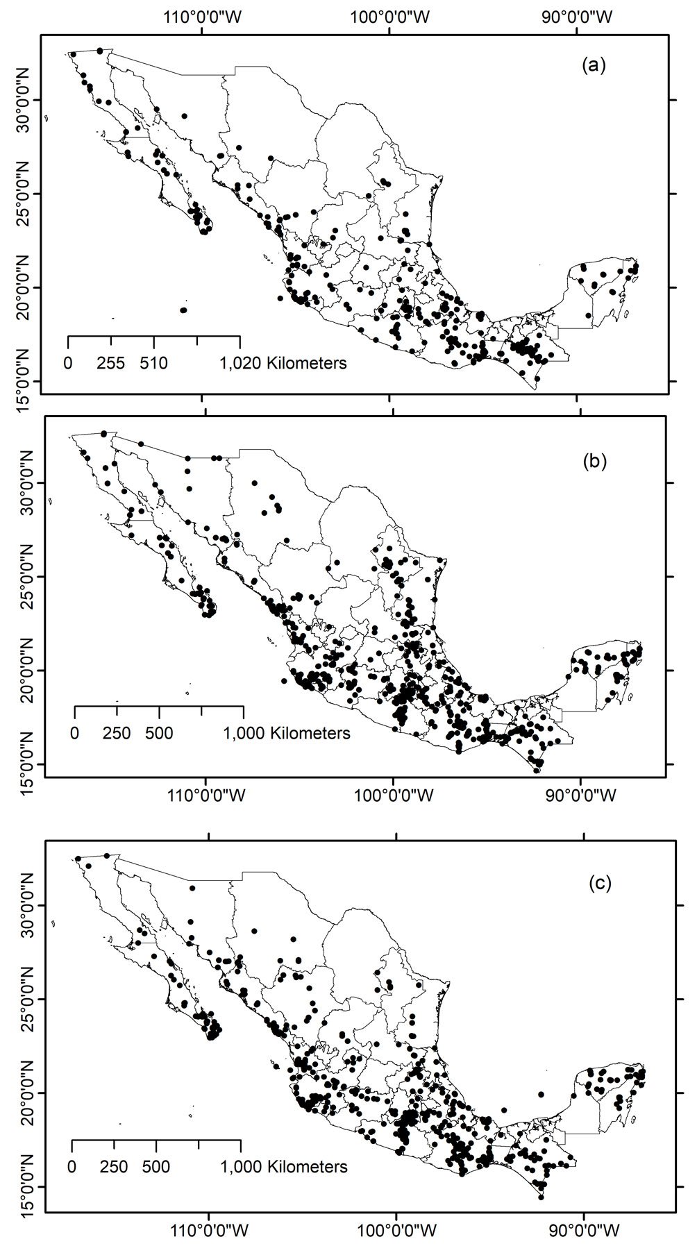
Table 1
Number of Cerambycidae species by state in Mexico.
| State | Species |
| Baja California | 38 |
| Baja California Sur | 62 |
| Campeche | 8 |
| Chiapas | 92 |
| Chihuahua | 8 |
| Coahuila | 4 |
| Colima | 22 |
| Mexico City | 3 |
| Durango | 15 |
| Guanajuato | 2 |
| Guerrero | 67 |
| Hidalgo | 14 |
| Jalisco | 96 |
| Estado de México | 25 |
| Michoacan | 27 |
| Morelos | 45 |
| Nayarit | 49 |
| Nuevo Leon | 17 |
| Oaxaca | 104 |
| Puebla | 36 |
| Queretaro | 3 |
| Quintana Roo | 30 |
| San Luis Potosi | 24 |
| Sinaloa | 47 |
| Sonora | 16 |
| Tabasco | 3 |
| Tamaulipas | 22 |
| Tlaxcala | 1 |
| Veracruz | 66 |
| Yucatan | 33 |
| Zacatecas | 7 |
According to the maxent modelling, some variables showed almost the total contribution percentage in model prediction: For instance, the precipitation of driest month (wc_bio14) had 94% contribution in predicting Phaea acromela and 87% contribution in predicting Eburia brevispinis potential distributions. Similarly, precipitation seasonality (wc_bio15) contributed 79% and 76% for modeling Neocompsa puncticollis asperula and Psyrassa cylindricollis potential distributions, respectively. Other high contribution percentages included: precipitation of wettest month (wc_bio13) had 73% contribution predicting Lagocheirus binumeratus; wc_bio15 had 71% contribution predicting Neocompsa alacris; temperature annual range (wc_bio7) had 71% contribution predicting Lagocheirus araneiformis ypsilon; isothermality (wc_bio3) had 70% contribution predicting Tetraopes umbonatus; wc_bio14 had 61% contribution predicting Lagocheirus procerus; and elevation had 60% contribution predicting Tetraopes femoratus.

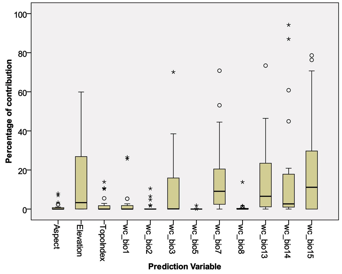
Table 2
Selected prediction variables.
| Bioclimatic variables | |
| wc_bio1 = Annual Mean Temperature | |
| wc_bio2 = Mean Diurnal Range (Mean of monthly [max temp – min temp]) | |
| wc_bio3 = Isothermality (BIO2/BIO7) (×100) | |
| wc_bio5 = Max Temperature of Warmest Month | |
| wc_bio7 = Temperature Annual Range (BIO5-BIO6) | |
| wc_bio8 = Mean Temperature of Wettest Quarter | |
| wc_bio13 = Precipitation of Wettest Month | |
| wc_bio14 = Precipitation of Driest Month | |
| wc_bio15 = Precipitation Seasonality (Coefficient of Variation) | |
| Topographic variables | |
| Elevation | |
| Aspect | |
| Topographic Index |
Considering prediction variables with high contribution percentages for multiple species models, Figure 3 and Table 3 show the most important variables: wc_bio15 (mean = 19%), wc_bio14 (mean = 17%), wc_bio7 (mean = 16%), wc_bio13 (mean = 15%), elevation (mean = 14%), and wc_bio3 (mean = 10%). On the other hand, those prediction variables that had low contribution percentages for fewer species included: Max temperature of warmest month (wc_bio5, mean = 0.09%), mean temperature of wettest quarter (wc_bio8, mean = 0.80%), aspect (mean = 1.06%), mean diurnal range (wc_bio2, mean = 1.07%), topoindex (mean = 2.3%), annual mean temperature (wc_bio1, mean=2.9).
The 4 prediction algorithms, Maximum Entropy (Maxent), Support Vector Machine (SVM), Generalized Linear Model (GLM), and Artificial Neural Networks (ANN) were applied to each of the 24 species that have ≥ 20 records. The models obtained consisted of probability approximations generated by both Modeco and Maxent (ClogLog). The different models for each species were combined by calculating the median value. Then, model accuracy was obtained by calculating the partial ROC test with 500 simulations. These results are shown in Table 4.
In general, the modeled species exhibited high mean AUC ratios and high mean partial AUC values, indicating good model performance, as values of 2.0 and 1.0, respectively, represent a perfect model fit. Mean AUC ratios varied between 1.51 and 1.97, and partial AUC values varied between 0.75 and 0.98. Species with very high mean AUC ratios (> 1.9) included Lagocheirus binumeratus, Psyrassa cylindricollis, Psyrassa sthenias, Neocompsa alacris, Eburia nigrovittata, Euderces batesi. On the other hand, the species with the lowest mean AUC ratios (> 1.5 and < 1.7) were Susuacanga ulkei, Dylobolus rotundicollis, and Tetraopes discoideus.
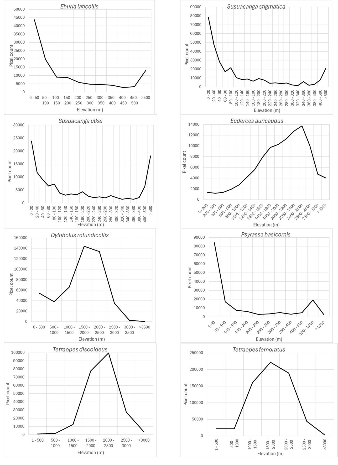
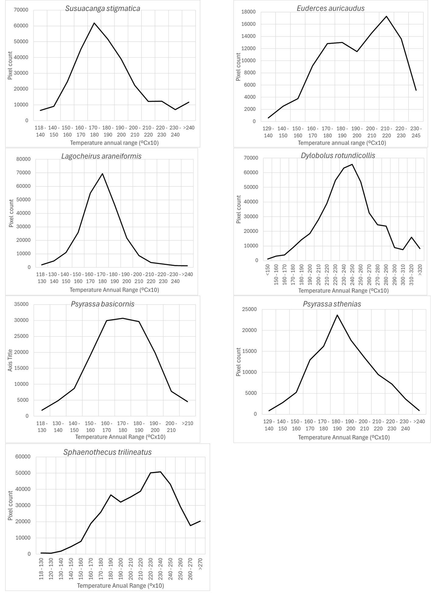
Based on the most important prediction variables identified by the Maxent algorithm, the response variables corresponding to each species model are shown in figures 4-9. For the elevation variable, there were species that preferred elevations between 0 and 50 m: Eburia laticollis, Susuacanga stigmatica, Psyrassa basicornis, and Susuacanga ulkei, which also showed significant predicted areas with elevations above 500 m. On the other hand, there were species selecting distribution areas at much higher elevations: Dylobolus rotundicollis and Tetraopes femoratus at 1,500-2,000 m, Tetraopes discoideus at 2,000-2,500 m, and Euderces auricaudus at 2,400-2,600 m (Fig. 4).
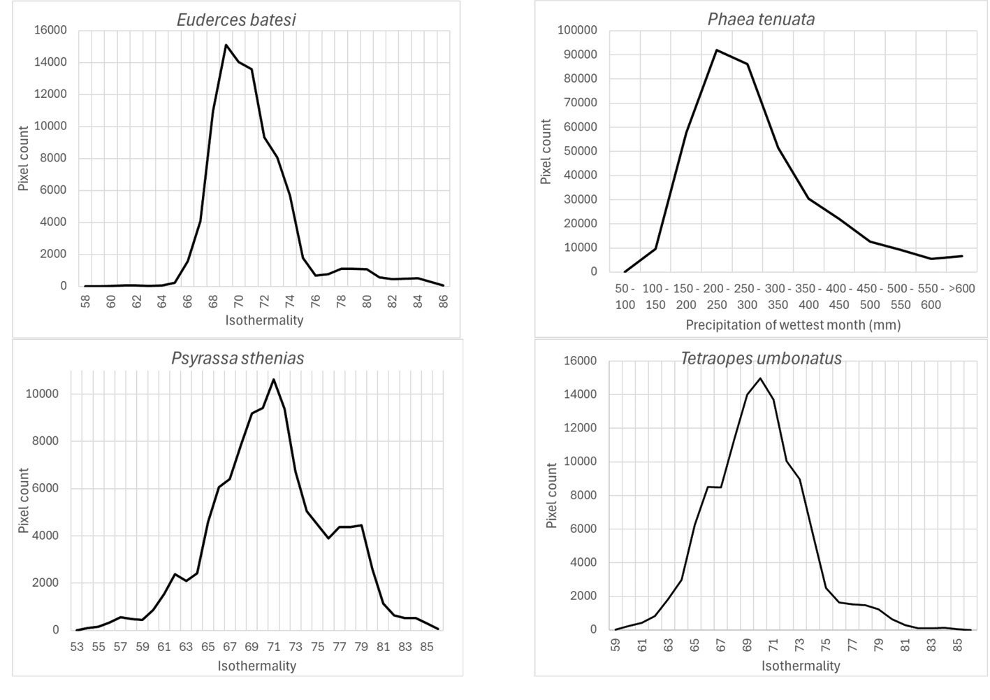
Isothermality (wc_bio3), which is an indicator of daily temperature variation with respect to annual temperature variation, had preferred values < 100 for species models built with this variable as important (35-70%): Highest preferred isothermality values were similar for different species models: Phaea tenuata (65), Euderces batesi (69), Tetraopes umbonatus (70), and Psyrassa sthenias (71) (Fig. 5).
According to Maxent, temperature annual ranges (wc_bio7) were also an important prediction variable for species with different preferring values: 3 species models (Susuacanga stigmatica, Lagocheirus araneiformis, and Psyrassa basicornis) showed temperature annual ranges preferred at 170-180 mm, while Psyrassa sthenias preferred the 18-19ᵒC range. Other species models showed preference for higher temperature annual ranges (Fig. 6): Euderces auricaudus (21-22 ᵒC), Sphaenothecus trilineatus (23-24 ᵒC) and Dylobolus rotundicollis (24-25 ᵒC).
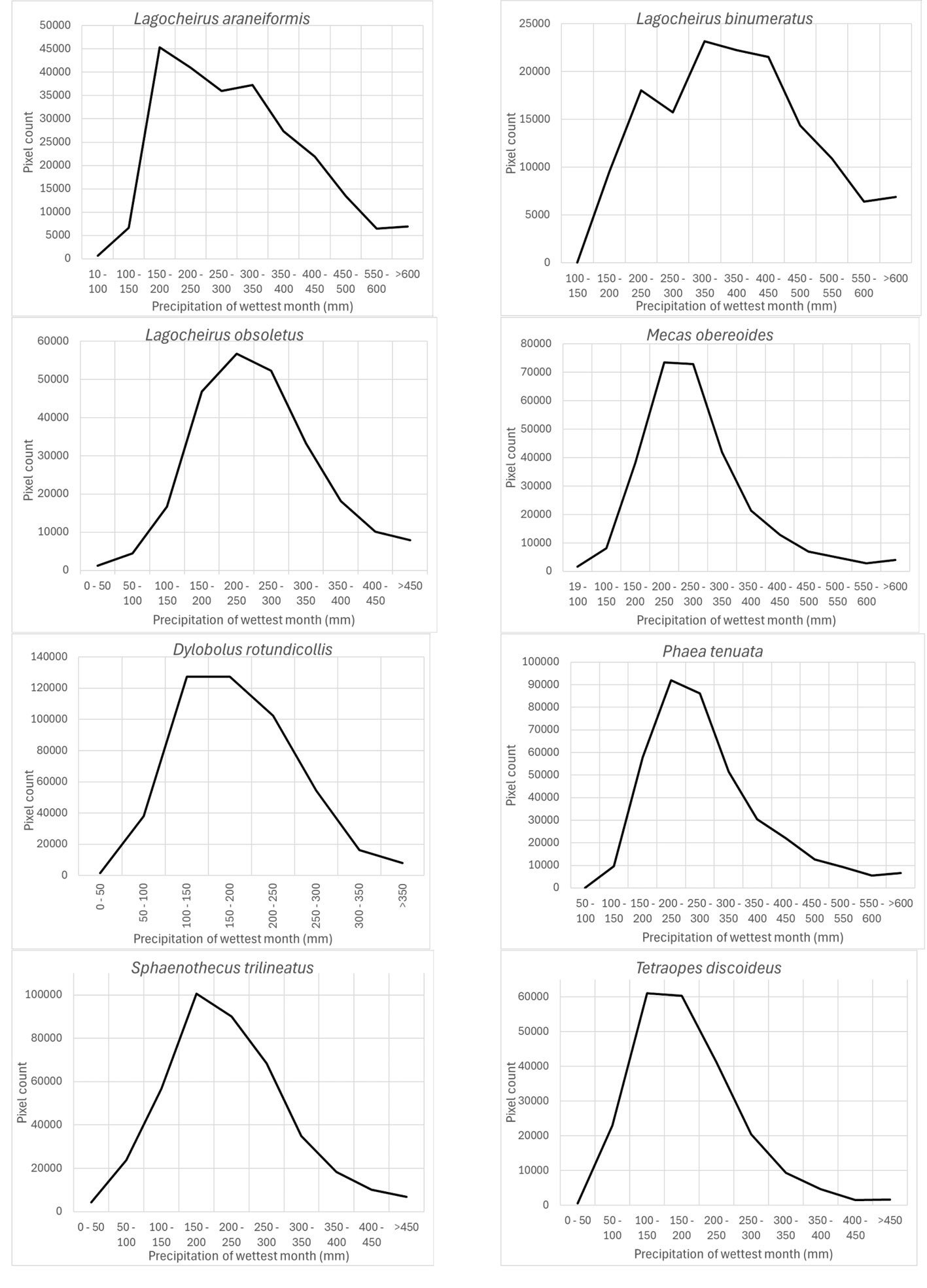
Precipitation of the wettest month (wc_bio13) was another important prediction variable whose highest preferred values varied according to different species: Lagocheirus araneiformis, Dylobolus rotundicollis, Sphaenothecus trilineatus, and Tetraopes discoideus at 150-200 mm; Lagocheirus obsoletus, Mecas obereoides, Phaea tenuata at 200-250 mm; and Lagocheirus binumeratus at 300-350 mm (Fig. 7).
Table 3
Percentage of contribution of each variable in the elaboration of distribution models by the Maxtent algorithm.
| Species | aspect | elevation | topoindex | wc_bio1 | wc_bio2 | wc_bio3 | wc_bio5 | wc_bio7 | wc_bio8 | wc_bio13 | wc_bio14 | wc_bio15 |
| Eburia brevispinis | 0.5 | 0 | 0 | 0 | 4.8 | 0 | 0 | 7.8 | 0 | 0 | 87 | 0 |
| E. laticollis | 0 | 27.4 | 0 | 25.7 | 0 | 0 | 0 | 1.9 | 0 | 0.3 | 11.3 | 33.4 |
| E. nigrovittata | 0 | 0 | 0 | 26.5 | 0 | 0 | 0 | 10.4 | 0 | 2 | 13.5 | 47.6 |
| Susuacanga stigmatica | 0 | 50.2 | 0 | 2.7 | 0 | 0 | 0 | 35.9 | 1.5 | 9.8 | 0 | 0 |
| S. ulkei | 0.1 | 25.8 | 0 | 0 | 0.1 | 2.2 | 0 | 0 | 13.8 | 0 | 44.9 | 13.2 |
| Euderces auricaudus | 0 | 30.7 | 0 | 0 | 0 | 15.3 | 0 | 53.1 | 0.5 | 0 | 0.4 | 0 |
| E. batesi | 0.5 | 24.2 | 0 | 0 | 0 | 35.1 | 1.8 | 19.8 | 0.3 | 15.4 | 3 | 0 |
| Lagocheirus araneiformis ypsilon | 0.3 | 0.1 | 5.5 | 0 | 1.7 | 0 | 0.1 | 70.8 | 0 | 21.1 | 0 | 0.4 |
| L. binumeratus | 7.9 | 0.7 | 0 | 0 | 0 | 0.3 | 0.1 | 17.5 | 0 | 73.4 | 0 | 0 |
| L. obsoletus | 0 | 1.2 | 2.9 | 1 | 0 | 6.1 | 0 | 15.3 | 0 | 46.4 | 16.2 | 10.9 |
| L. procerus | 0 | 4.7 | 0 | 1.4 | 6.5 | 0 | 0 | 1.8 | 0.4 | 13.1 | 60.8 | 11.4 |
| Mecas obereoides | 0 | 0 | 0 | 2.2 | 0 | 0 | 0 | 15.3 | 0 | 37.3 | 1.6 | 43.5 |
| Dylobolus rotundicollis | 0 | 27.1 | 10.3 | 0 | 0 | 0 | 0 | 20.3 | 1.1 | 22.6 | 18.5 | 0 |
| Neocompsa alacris | 0 | 1.9 | 10.7 | 5.3 | 0 | 0 | 0 | 5.6 | 0 | 3.6 | 2.1 | 70.7 |
| N. puncticollis asperula | 7 | 0 | 0 | 0 | 2 | 0 | 0 | 4.7 | 0 | 3.3 | 4.4 | 78.6 |
| Phaea acromela | 3.3 | 0 | 0 | 0 | 0 | 0.2 | 0 | 0 | 0 | 2.4 | 94.2 | 0 |
| P. tenuata | 2.4 | 6.3 | 0.5 | 0 | 0 | 38.5 | 0 | 3.4 | 0 | 43.4 | 2 | 3.5 |
| Psyrassa basicornis | 0 | 26.6 | 0 | 5.3 | 0.1 | 16.5 | 0 | 44.5 | 1.6 | 5.3 | 0.1 | 0 |
| P. cylindricollis | 1 | 9 | 0.6 | 0 | 0 | 0 | 0.1 | 3 | 0 | 7.8 | 2.1 | 76.3 |
| P. sthenias | 2.4 | 0.6 | 0 | 0 | 0 | 35.5 | 0 | 20.7 | 0 | 4.5 | 17.2 | 19.1 |
| Sphaenothecus trilineatus | 0 | 0 | 0.4 | 0.2 | 0 | 14.4 | 0 | 27 | 0 | 25.1 | 20.9 | 12 |
| Tetraopes discoideus | 0 | 41.2 | 10.5 | 0 | 0 | 16.5 | 0 | 1.2 | 0 | 24.3 | 2.3 | 4.1 |
| T. femoratus | 0 | 59.9 | 13.9 | 0 | 10.5 | 0 | 0 | 0 | 0 | 0 | 2.3 | 13.4 |
| T. umbonatus | 0 | 0.4 | 0 | 0 | 0 | 70.1 | 0 | 3.5 | 0 | 0 | 0 | 26 |
| Mean | 1.06 | 14.08 | 2.30 | 2.93 | 1.07 | 10.45 | 0.09 | 15.98 | 0.80 | 15.05 | 16.87 | 19.34 |
| Median | 0.00 | 3.30 | 0.00 | 0.00 | 0.00 | 0.10 | 0.00 | 9.10 | 0.00 | 6.55 | 2.65 | 11.15 |
| Standard deviation | 2.17 | 18.15 | 4.35 | 7.31 | 2.60 | 17.81 | 0.37 | 18.62 | 2.81 | 18.89 | 27.21 | 25.63 |
Table 4
Partial ROC results for modeled species.
| Species | Mean AUC ratio | Mean partial AUC |
| Eburia brevispinis | 1.884237 | 0.9420767 |
| E. laticollis | 1.857125 | 0.9285514 |
| E. nigrovittata | 1.939383 | 0.9696851 |
| Susuacanga stigmatica | 1.738087 | 0.869013 |
| S. ulkei | 1.512725 | 0.7563525 |
| Euderces auricaudus | 1.822893 | 0.9114264 |
| E. batesi | 1.972096 | 0.9860455 |
| Lagocheirus araneiformis ypsilon | 1.789459 | 0.8944192 |
| L. binumeratus | 1.909858 | 0.9549165 |
| L. obsoletus | 1.772241 | 0.886116 |
| L. procerus | 1.749532 | 0.8747619 |
| Mecas obereoides | 1.767577 | 0.8837588 |
| Dylobolus rotundicollis | 1.664294 | 0.8320284 |
| Neocompsa alacris | 1.938096 | 0.9690422 |
| N. puncticollis asperula | 1.883306 | 0.9416244 |
| Phaea acromela | 1.866931 | 0.9334454 |
| P. tenuata | 1.776351 | 0.888124 |
| Psyrassa basicornis | 1.871859 | 0.9359075 |
| P. cylindricollis | 1.919474 | 0.9597301 |
| P. sthenias | 1.921234 | 0.9606008 |
| Sphaenothecus trilineatus | 1.876181 | 0.9380483 |
| Tetraopes discoideus | 1.680489 | 0.8401879 |
| T. femoratus | 1.815506 | 0.907635 |
| T. umbonatus | 1.707098 | 0.8535488 |
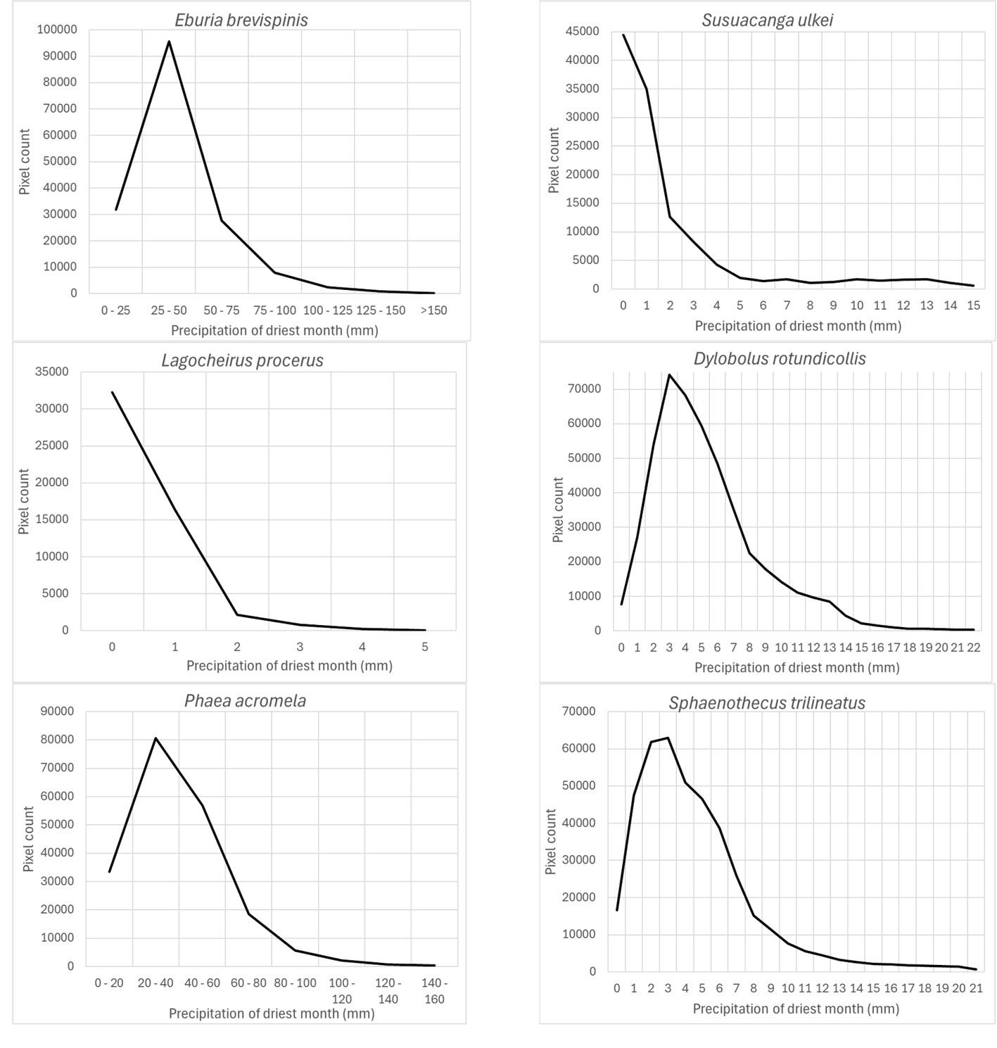
The precipitation of the driest month (wc_bio14) was also an important prediction variable for which its response variable took the highest preferred values between 0 and 25-50 mm: Susuacanga ulkei and Lagocheirus procerus showed the highest preferred values of 0 mm, Dylobolus rotundicollis and Sphaenothecus trilineatus at 3 mm, and Eburia brevispinis and Phaea acromela at 25-50 mm (Fig. 8).
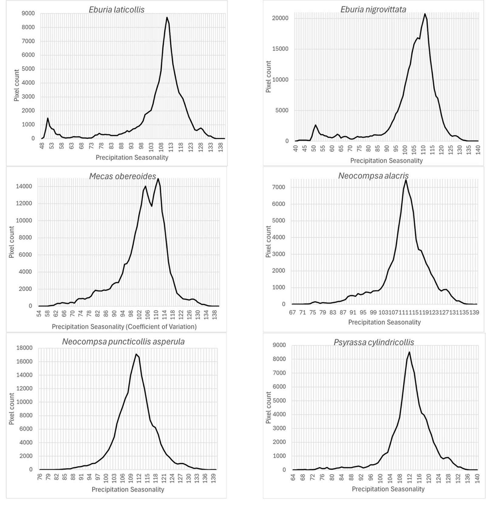
Finally, the precipitation seasonality (wc_bio15), which is the coefficient of variation of precipitation, was an important prediction variable whose preferred highest values (110) seem similar for this group of species (Fig. 9): Eburia laticollis, Eburia nigrovittata, Mecas obereoides, Neocompsa alacris, Neocompsa puncticollis asperula, and Psyrassa cylindricollis.
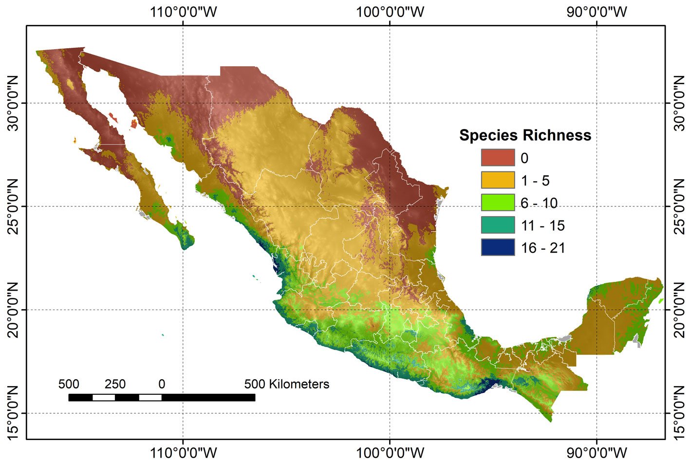
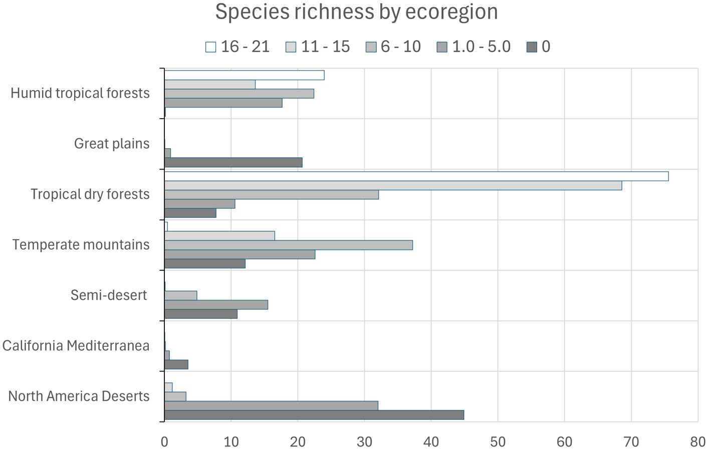
A composite map was generated by adding each of 24 binary species distribution models (Fig. 10). In general, species that highly concurred (16-21 spp.) in only 2 very confined areas, located in southern Sinaloa and southern Oaxaca. On the other hand, large areas with no species concurring were in northern Mexico (Fig. 10). This richness map was cross-tabulated with the ecoregion map to show the biomes associated with the different concurring intervals (Fig. 11). Each richness interval was tabulated for different ecoregions, showing that the highest range (16-21 spp.) corresponded to the tropical dry forest in 75% and the tropical humid forest in 24%. The second highest interval (11-15 spp.) corresponded again to the tropical dry forest (69%), but this time, the temperate mountains were in the second place with 17%, and the tropical humid forest with 14%. On the other hand, the areas with no species concurrence corresponded to the North American Desert (45%), followed by the Great Plains (21%), temperate mountains (12%), and semi-desert (11%). The tropical dry forest occupied 8% of such areas with no species concurrence, while the tropical humid forest occupied only 0.2%.
Discussion
Considering the original number of records included in the databases (> 10,000) along with the localities, both georeferenced and without geographic coordinates, and the number of species, there was the expectation to obtain a database with a significant number of species and records. However, there existed a very limited number of species (24) with enough records (≥ 20) to be used in modeling species potential distribution. In fact, the species with ≥ 5 and < 20 records were also limited (124), and the bulk of species (266) had < 5 records (Supplementary material: A2). It is evident that extensive taxonomic fieldwork is necessary to document the species diversity of Cerambycidae in Mexico. In this regard, and apparently supporting this pattern of records, 7.4% of the species recorded in Mexico have no locality records in the country, 45.5% have been recorded in only one state, and 16% in 2 states. This means that nearly 69% of the species have either a restricted distribution or are poorly studied in terms of their distribution (F. A. Noguera, unpublished data).
By mapping the geographic location of Cerambycidae species records in Mexico, it is noteworthy that the sampling intensity does not necessarily reflect the intensity of sampling, as the information included primarily corresponds to taxonomically studied groups rather than studies aimed at documenting the diversity of the different regions of the country, and sampling gaps are revealed by state and ecoregion across the country. In fact, the map somewhat confirms the current knowledge about the diversity of this group in the various states of the republic (Martínez-Hernández et al., 2024; Noguera, 2014; Noguera unpublished data). For example, in fact, 565 species have been recorded in Oaxaca, 485 in Veracruz, 435 in Chiapas, 397 in Jalisco, 283 in Guerrero, and 216 in Morelos —states with the highest number of records included in the study. In contrast, states such as Tlaxcala (10 species), Campeche (11), Aguascalientes (12), Tabasco (21), Zacatecas (26), Guanajuato (33), Coahuila (35), Mexico City (36), Nuevo León (69), and Chihuahua (73) recorded the fewest species in this study.
In the ≥ 20 records per species group, the most sampled biome was the tropical dry forest (348 records and 23 species), while the temperate forests included 21 species with 140 records.
The 24 species distribution models primarily represent examples of this family’s species that are better sampled in the country. Different from relying on a single prediction algorithm, this study presents consensus models, generated from combining probability versions of 4 algorithms: Maxent, Artificial Neural Networks, Generalized Linear Model, and Support Vector Machine. The median was the statistic chosen for combining the 4 algorithms because of its characteristic of being a location parameter in contrast with the mean, which combines in-depth partial values, and is affected by outliers. Although the variations among models for the same species were evident, all 24 species distribution models showed good performance, as indicated by the AUC ratios and partial AUC values.
According to Maxent, prediction variables differed in importance for predicting species potential distribution models. The variables that had higher mean importance among species included precipitation seasonality (wc_bio15), precipitation of driest month (wc_bio14), temperature annual range (wc_bio7), precipitation of wettest month (wc_bio13), elevation, and isothermality (wc_bio3). As in this case, other studies on Cerambycidae, where the potential distribution of some species in this group was modeled, also showed that the predictive bioclimatic variables were diverse and contributed to the models to varying degrees. For example, for Psacothea hilaris, the predictive variables were precipitation of the warmest quarter (wc_bio18) and isothermality (wc_bio3) (Ruzzier et al., 2024); for Rosalia alpina, they were elevation and mean temperature of the driest quarter (wc_bio9) (Bosso et al., 2018); for Morimus asper, they were the maximum temperature during the warmest month (wc_bio5) and altitude (Kostova et al., 2023); for Batocera lineolata, they were maximum temperature in January, precipitation in July, and temperature seasonality (wc_bio4) (Li et al., 2020); for Xylotrechus arvicola, they were precipitation in October, mean maximum temperature in January, mean minimum temperature in July, mean maximum temperature, and mean minimum temperature in August (Felicísimo et al., 2021); for Monochamus carolinensis, they were precipitation of the warmest quarter (wc_bio18), precipitation seasonality (wc_bio15), precipitation of the coldest quarter (wc_bio19), mean diurnal range (wc_bio2), and minimum temperature of the coldest month (wc_bio5) (Zhao et al., 2023). This recorded variety in predictive environmental variables corresponds to the region where each of these studies was conducted. For P. hilaris, the main areas were Italy and the Mediterranean region; for R. alpina, it was Europe; for M. asper, it was Bulgaria; for B. lineolata, it was China; for X. arvicola, it was Spain; and for M. carolinensis, it was on a global scale.
The response variables obtained by cross-tabulating the species presence models with the environmental (prediction) variables identify the most favorable habitat conditions, according to the predicted distribution models. Even though the most frequent values of the environmental variables indicate which areas dominated the species distribution, the range of such values provides an estimate of the span of environmental values where species can occur.
The 24 modeled species showed spatial correspondence, where the highest interval (16-21 species) is confined to restricted areas with tropical and humid tropical forests in the country. Larger species spatial correspondence areas corresponded to the lowest intervals (1-5 and 6-10 species), which were distributed in the tropical dry forest and temperate forests. It is worth mentioning that biomes such as the North American deserts and the Great Plains showed the highest proportion of areas with the absence of species.
References
Anderson, R. P., & Martı́nez-Meyer, E. (2004). Modeling species’ geographic distributions for preliminary conservation assessments: an implementation with the spiny pocket mice (Heteromys) of Ecuador. Biological Conservation, 116, 167–179. https://doi-org.pbidi.unam.mx:2443/10.1016/S0006-3207(03)00187-3
Araújo, M. B., & New, M. (2007). Ensemble forecasting of species distributions. Trends in Ecology & Evolution, 22, 42–47. https://doi.org/10.1016/j.tree.2006.09.010
Austin, M. P. (2002). Spatial prediction of species distribution: an interface between ecological theory and statistical modelling. Ecological Modelling, 157, 101–118. https://doi.org/10.1016/S0304-3800(02)00205-3
Ballesteros-Mejia, L., Kitching, I. J., Jetz, W., Nagel, P., & Beck, J. (2013). Mapping the biodiversity of tropical insects: species richness and inventory completeness of African sphingid moths. Global Ecology and Biogeography, 22, 586–595. https://doi.org/10.1111/geb.12039
Ballesteros-Mejia, L., Kitching, I. J., Jetz, W., & Beck, J. (2017). Putting insects on the map: near-global variation in sphingid moth richness along spatial and environmental gradients. Ecography, 40, 698–708. https://doi.org/10.1111/ecog.02438
Barredo, J. I., Strona, G., De Rigo, D., Caudullo, G., Stancanelli, G., & San-Miguel-Ayanz, J. (2015). Assessing the potential distribution of insect pests: case studies on large pine weevil (Hylobius abietis L) and horse-chestnut leaf miner (Cameraria ohridella) under present and future climate conditions in European forests. EPPO Bulletin, 45, 273–281. https://doi.org/10.1111/epp.12208
Bezark, L. G., & Monné, M. A. (2013). Checklist of the Oxypeltidae, Vesperidae, Disteniidae and Cerambycidae, (Coleoptera) of the Western Hemisphere. Retrieved from: http://bezbycids.com/byciddb/checklists/WestHemiCerambycidae2024.pdf
Bosso, L., Smeraldo, S., Rapuzzi, P., Sama, G., & Garonna, A. P. (2018). Nature protection areas of Europe are insufficient to preserve the threatened beetle Rosalia alpina (Coleoptera: Cerambycidae): evidence from species distribution models and conservation gap analysis. Ecological Entomology, 43, 192–203. https://doi.org/10.1111/een.12485
Buse, J., Schröder, B., & Assmann, T. (2007). Modelling habitat and spatial distribution of an endangered longhorn beetle-A case study for saproxylic insect conservation. Biological Conservation, 137, 372–381. https://doi.org/10.1016/j.biocon.2007.02.025
Catalano, G. A., D’Urso, P. R., Maci, F., & Arcidiacono, C. (2023). Influence of parameters in SDM application on citrus presence in mediterranean area. Sustainability, 15, 7656. https://doi.org/10.3390/su15097656
Crawford, P. H. C., & Hoagland, B. W. (2010). Using species distribution models to guide conservation at the state level: the endangered American burying beetle (Nicrophorus americanus) in Oklahoma. Journal of Insect Conservation, 14, 511–521. https://doi.org/10.1007/s10841-010-9280-8
Colwell, R. K. (1996). Biota: the biodiversity database manager. Sinauer Associates, Sunderland, Massachusetts. Systematic Biology, 46, 574–575.
D’Amen, M., Pradervand, J. N., & Guisan, A. (2015). Predicting richness and composition in mountain insect communities at high resolution: a new test of the SESAM framework. Global Ecology and Biogeography, 24, 1443–1453. https://doi.org/10.1111/geb.12357
Drake, J. M., Randin, C., & Guisan, A. (2006). Modelling ecological niches with support vector machines. Journal of Applied Ecology, 43, 424–432. https://doi.org/10.1111/
j.1365-2664.2006.01141.x
Elith, J., Graham, C. H., Anderson, R. P., Dudík, M., Ferrier, S., Guisan, A. et al. (2006). Novel methods improve prediction of species’ distributions from occurrence data. Ecography,
29, 129–151. https://doi.org/10.1111/j.2006.0906-7590.04596.x
Eickermann, M., Junk, J., & Rapisarda, C. (2023). Climate change and insects. Insects, 14, 678. https://doi.org/10.3390/insects14080678
Elith, J., & Graham, C. H. (2009). Do they? How do they? Why do they differ? On finding reasons for differing performances of species distribution models. Ecography, 32, 66–77. https://doi.org/10.1111/j.1600-0587.2008.05505.x
Felicísimo, A. M., Armendáriz, I., & Alberdi, V. (2021). Modelling the potential effects of climate change in the distribution of Xylotrechus arvicola in Spain. Horticultural Science (Prague), 48, 38–46. https://doi.org/10.17221/85/2019-HORTSCI
Fick, S. E., & Hijmans, R. J. (2017). WorldClim 2: new 1-km spatial resolution climate surfaces for global land areas. International Journal of Climatology, 37, 4302–4315. https://doi.org/10.1002/joc.5086
Franklin, J. (2010). Mapping species distributions. Spatial inference and prediction. Cambridge UK: Cambridge University Press. https://doi.org/10.1017/CBO9780511810602
Graham, C. H., Ferrier, S., Huettman, F., Moritz, C., & Peterson, A. T. (2004). New developments in museum-based informatics and applications in biodiversity analysis. Trends in Ecology & Evolution, 19, 497–503. https://doi.org/10.1016/j.tree.2004.07.006
Guisan, A., & Zimmermann, N. E. (2000). Predictive habitat distribution models in ecology. Ecological Modelling, 135, 147–186. https://doi.org/10.1016/S0304-3800(00)00354-9
Guisan, A., Edwards, T. C., & Hastie, T. (2002). Generalized linear and generalized additive models in studies of species distributions: setting the scene. Ecological Modelling, 157, 89–100. https://doi.org/10.1016/S0304-3800(02)00204-1
Guo, Q., Kelly, M., & Graham, C. H. (2005). Support vector machines for predicting distribution of Sudden Oak Death in California. Ecological Modelling, 182, 75–90. https://doi.org/10.1016/j.ecolmodel.2004.07.012
Guo, Q., & Liu, Y. (2010). ModEco: an integrated software package for ecological niche modeling. Ecography, 33, 637–642. https://doi.org/10.1111/j.1600-0587.2010.06416.x
Hassall, C. (2012). Predicting the distributions of under-recorded Odonata using species distribution models. Insect Conservation and Diversity, 5, 192–201. https://doi.org/10.1111/j.1752-4598.2011.00150.x
Hastie, T., Tibshirani, R., & Friedman, J. (2001). The elements of statistical learning: data mining, inference, and prediction.
New York: Springer. https://doi.org/10.1007/978-0-387-21606-5
Hijmans, R. J., Cameron, S. E., Parra, J. L., Jones, P. G., & Jarvis, A. (2005). Very high resolution interpolated climate surfaces for global land areas. International Journal of Climatology: A Journal of the Royal Meteorological Society, 25, 1965–1978. https://doi.org/10.1002/joc.1276
Huntley, B., Green, R. E., Collingham, Y. C., Hill, J. K., Willis, S. G., Bartlein, P. J. et al. (2004). The performance of models relating species geographical distributions to climate is independent of trophic level. Ecology Letters, 7, 417–426. https://doi.org/10.1111/j.1461-0248.2004.00598.x
Jung, J. M., Lee, W. H., & Jung, S. (2016). Insect distribution in response to climate change based on a model: Review of function and use of CLIMEX. Entomological Research, 46, 223–235. https://doi.org/10.1111/1748-5967.12171
Kostova, R., Bekchiev, R., Popgeorgiev, G., & Kornilev, Y. V. (2023). First exhaustive distribution and habitat modelling of Morimus asper (Sulzer, 1776) sensu lato (Coleoptera, Cerambycidae) in Bulgaria. Nature Conservation, 53, 39–59. https://doi.org/10.3897/natureconservation.53.104243
Lek, S., Delacoste, M., Baran, P., Dimopoulos, I., Lauga, J., & Aulagnier, S. (1996). Application of neural networks to modelling nonlinear relationships in ecology. Ecological Modelling,90, 39–52. https://doi.org/10.1016/0304-3800(95)00142-5
Li, A., Wang, J., Wang, R., Yang, H., Yang, W., Yang, C. et al. (2020). MaxEnt modeling to predict current and future distributions of Batocera lineolata (Coleoptera: Cerambycidae) under climate change in China. Écoscience, 27, 23–31. https://doi.org/10.1080/11956860.2019.1673604
Linsley, E. G. (1961). The Cerambycidae of North America. Part I. Introduction. University of California Publications in Entomology, 18, 1–135.
Lobo, J. M. (2016). The use of occurrence data to predict the effects of climate change on insects. Current Opinion in Insect Science, 17, 62–68. https://doi.org/10.1016/j.cois.
2016.07.003
Lobo, J. M., Lumaret, J. P., & Jay-Robert, P. (2002). Modelling the species richness distribution of French dung beetles (Coleoptera, Scarabaeidae) and delimiting the predictive capacity of different groups of explanatory variables. Global Ecology and Biogeography, 11, 265–277. https://doi.org/10.1046/j.1466-822X.2002.00291.x
Ma, G., & Ma, C. S. (2022). Potential distribution of invasive crop pests under climate change: incorporating mitigation responses of insects into prediction models. Current
Opinion in Insect Science, 49, 15–21. https://doi.org/10.1016/j.cois.2021.10.006
Martínez-Hernández, J. G., Rös, M., Pérez-Flores, O., & Toledo-Hernández, V. H. (2024). Checklist of the Cerambycidae (Coleoptera: Chrysomeloidea) of Oaxaca, Mexico. Zootaxa, 5405, 185–208. https://doi.org/10.11646/zootaxa.5405.2.2
Monné, M. A. (2005). Catalogue of the Cerambycidae (Coleoptera) of the Neotropical region. Part I. Subfamily Cerambycinae. Zootaxa, 946, 17–65. https://doi.org/10.11646/zootaxa.946.1.1
Müller, K. R., Mika, S., Tsuda, K., & Schölkopf, K. (2002). An introduction to Kernel-based learning algorithms. In Yu Hen Hu, & Jenq-Neng Hwang (Eds.), Handbook of neural network signal processing. Boca-Raton: CRC Press. https://doi.org/10.1201/9781315220413
Nearns, E. H., Lord, N. P., Lingafelter, S. W., Santos, A., Miller, K. B., & Zaspel, J. M. (2017). LONGICORN ID. Retrieved from: https://cerambycids.com
Noguera, F. A. (2014). Biodiversidad de Cerambycidae (Coleoptera) en México. Revista Mexicana de Biodiversidad, 85 (Supl.), S290–S297. https://doi.org/10.7550/rmb.32966
Norberg, A., Abrego, N., Blanchet F. G., Adler, F. R., Anderson, B. J., Anttila, J. et al. (2019). A comprehensive evaluation of predictive performance of 33 species distribution models at species and community levels. Ecological Monographs, 89, e01370. https://doi.org/10.1002/ecm.1370
Peterson, A. T., Papeş, M., & Soberón, J. (2008). Rethinking receiver operating characteristic analysis applications in ecological niche modeling. Ecological Modelling, 213, 63–72. https://doi.org/10.1016/j.ecolmodel.2007.11.008
Phillips, S. J., Anderson, R. P., & Schapire, R. E. (2006). Maximum entropy modeling of species geographic distributions. Ecological Modelling, 190, 231–259. https://doi.org/10.1016/j.ecolmodel.2005.03.026
Phillips, S. J., Anderson, R. P., Dudík, M., Schapire, R. E., & Blair, M. E. (2017). Opening the black box: an open-source release of Maxent. Ecography, 40, 887–893. https://doi.org/10.1111/ecog.03049
Phillips, S. J., & Dudík, M. (2008). Modeling of species distributions with Maxent: new extensions and a comprehensive evaluation. Ecography, 31, 161–175. https://doi.org/10.1111/j.0906-7590.2008.5203.x
Pouteau, R., Meyer, J. Y., Taputuarai, R., & Stoll, B. (2012). Support vector machines to map rare and endangered
native plants in Pacific islands forests. Ecological Informatics, 9, 37–46. https://doi.org/10.1016/j.ecoinf.2012.03.003
Ruzzier, E., Lupi, D., Tirozzi, P., Dondina, O., Orioli V., Jucker, C. et al. (2024). A two‑step species distribution modeling to disentangle the effect of habitat and bioclimatic covariates on Psacothea hilaris, a potentially invasive species. Bio Invasions, 26, 1861–1881. https://doi.org/10.1007/s10530-024-03283-9
Schölkopf, B., Platt, J. C., Shawe-Taylor, J., Smola, A. J., & Williamson, R. C. (2001). Estimating the support of a high-dimensional distribution. Neural Computation, 13, 1443–1471. https://doi.org/10.1162/089976601750264965
Senay, S. D., & Worner, S. P. (2019). Multi-scenario species distribution modeling. Insects, 10, 65. https://doi.org/10.3390/insects10030065
Silva, D. P., Aguiar, A. G., & Simião-Ferreira, J. (2016). Assessing the distribution and conservation status of a long-horned beetle with species distribution models. Journal of Insect Conservation, 20, 611–620. https://doi.org/10.1007/s10841-016-9892-8
Toledo, V. H., & Corona, A. M. (2006). Patrones de distribución de la familia Cerambycidae (coleóptera). In J. J. Morrone, & J. Llorente Bosques (Eds.), Componentes bióticos principales de la entomofauna mexicana, México (pp. 425–474). México D.F.: Las Prensas de Ciencias, UNAM.
Ulrichs, C., & Hopper, K. R. (2008). Predicting insect distributions from climate and habitat data. BioControl, 53, 881–894. https://doi.org/10.1007/s10526-007-9143-8
Urbani, F., D’alessandro, P., & Biondi, M. (2017). Using Maximum Entropy Modeling (MaxEnt) to predict future trends in the distribution of high altitude endemic insects in response to climate change. Bulletin of Insectology, 70, 189–200.
Valavi, R., Guillera-Arroita, G., Lahoz-Monfort, J. J., & Elith, J. (2022). Predictive performance of presence-only species distribution models: a benchmark study with reproducible code. Ecological Monographs, 92, e01486. https://doi.org/10.1002/ecm.1486
Watts, M. J., & Worner, S. P. (2008). Comparing ensemble and cascaded neural networks that combine biotic and abiotic variables to predict insect species distribution. Ecological Informatics, 3, 354–366. https://doi.org/10.1016/j.ecoinf.2008.08.003
Williams, J. N., Seo, C., Thorne, J., Nelson, J. K., Erwin, S., O’Brien, J. M. et al. (2009). Using species distribution models to predict new occurrences for rare plants. Diversity and Distributions, 15, 565–576. https://doi.org/10.1111/j.1472-4642.2009.00567.x
Zaniewski, A. E., Lehmann, A., & Overton, J. M. (2002). Predicting species spatial distributions using presence-only data: a case study of native New Zealand ferns. Ecological Modelling, 157, 261–280. https://doi.org/10.1016/S0304-3800(02)00199-0
Zhao, J., Zou, X., Yuan, F., Luo, Y., & Shi, J. (2023). Predicting the current and future distribution of Monochamus carolinensis (Coleoptera: Cerambycidae) based on the maximum entropy model. Pest Management Science, 79, 5393–5404. https://doi.org/10.1002/ps.7753


