Vol. 88. núm. 1 (2017)
Marzo


Taxonomía y Sistemática
Ecología


Genetic diversity and phenotypic variation in a parasitoid wasp involved in the yucca – yucca moth interaction
C. Rocío Álamo-Herrera a, María Clara Arteaga a, *, Rafael Bello-Bedoy b
a Centro de Investigación Científica y de Educación Superior de Ensenada, Departamento de Biología de la Conservación, Carretera Tijuana-Ensenada # 3918, Zona Playitas, 22860 Ensenada, Baja California, Mexico
b Universidad Autónoma de Baja California, Facultad de Ciencias, Carretera Transpeninsular # 3917, Colonia Playitas, 22860 Ensenada, Baja California, Mexico
*Corresponding author: arteaga@cicese.mx (M.C. Arteaga)
Received: 28 February 2024; accepted: 01 July 2024
Abstract
Tri-trophic interactions between plants, herbivores, and parasitoids are a valuable model for studying how they influence the distribution of genetic diversity and phenotypic variability of the species involved. This study examines the taxonomic, morphological, and genetic diversity of parasitoid wasps involved in the Yucca–Tegeticula interaction on the Baja California Peninsula. We surveyed 35 locations across the peninsula and collected 119 parasitoid wasps. Of these, 114 were adults, while the remaining 5 were in the pupal stage. Our study identified 2 genera of wasps: Bassus sp. (Ichneumonidae; n = 8) and Digonogastra sp. (Brachonidae; n = 111). Moreover, we found moderate levels of genetic diversity within the Digonogastra population across the peninsula. Additionally, this population constitutes a single panmictic group with indications of historical demographic expansion. Phenotypically, we identified sexual dimorphism and variation associated with its different hosts and environmental heterogeneity Digonogastra’s geographical range.
Keywords: Baja California Peninsula; Genetic structure; Host-association; Morphometrics; Tri-trophic interactions
© 2024 Universidad Nacional Autónoma de México, Instituto de Biología. Este es un artículo Open Access bajo la licencia CC BY-NC-ND
(http://creativecommons.org/licenses/by-nc-nd/4.0/).
Diversidad genética y variación fenotípica en una avispa parasitoide involucrada en la interacción entre yucas y sus polillas polinizadoras
Resumen
Las interacciones tritróficas entre plantas, herbívoros y parasitoides son un modelo valioso para estudiar cómo influyen en la distribución de la diversidad genética y la variabilidad fenotípica de las especies involucradas. Este estudio examinó la diversidad taxonómica, morfológica y genética de avispas parasitoides en la interacción Yucca-Tegeticula en la Península de Baja California. El estudio se realizó en 35 localidades recolectando 119 avispas parasitoides; 114 adultos y 5 pupas. Se identificaron 2 géneros de avispas: Bassus sp. (Ichneumonidae; n = 8) y Digonogastra sp. (Brachonidae; n = 111). Se encontraron niveles moderados de diversidad genética dentro de la población de Digonogastra en toda la península, constituyendo un único grupo panmítico con indicios de expansión demográfica histórica. Fenotípicamente, identificamos dimorfismo sexual y variación asociada con sus diferentes hospederos y la heterogeneidad ambiental a lo largo de la distribución geográfica de Digonogastra.
Palabras clave: Península de Baja California; Estructura genética; Asociación al hospedero; Morfometría; Interacción tri-trófica
Introduction
Tritrophic interactions between plants, herbivores, and parasitoids have become pivotal to understanding species diversity (Abdala-Roberts et al., 2019; Godfray, 1994; Singer & Stireman, 2005). Parasitoids maintain an antagonistic relationship with insect herbivores by depositing their eggs inside or on them, ultimately leading to the death of their host (Godfray, 1994; Quicke, 2015; Resh & Cardé, 2009). These parasitoids serve as an indirect defense for plants, controlling herbivore population levels (Abdala-Roberts et al., 2019; Cuautle & Rico-Gray, 2003; Heil, 2008). Plants attract parasitoids by emitting chemical signals that indicate the presence of herbivores, which enables parasitoids to locate their prey, thus establishing mutually beneficial interactions (Heil, 2008; Kappers et al., 2011; Takabayashi & Dicke, 1996).
Multiple studies have explored how interactions among organisms affect the genetic and phenotypic variation within species (e.g., Agrawal, 2001; Carmona et al., 2015). For instance, biotic interactions may differ geographically, resulting in local selection processes and differentiation of parasitoid populations (Althoff & Thompson, 2001; Kankare et al., 2005; Stireman et al., 2005). Environmental factors or geographical distances can also determine the distribution of these variations (Althoff, 2008; Lozier et al., 2009; Stireman et al., 2005). For example, the genetic population structure of the wasp Cotesia congregata Say, 1836 (Hymenoptera: Braconidae) is related to the different plant-hosts with which it interacts (Karns, 2009). Conversely, genetic diversity in the parasitoid wasp Eusandalum sp. Ratzeburg, 1852 (Hymenoptera: Braconidae) is primarily associated with its broad geographical distribution rather than the species it interacts with (Althoff, 2008).
The interaction between Yucca Linnaeus plants, moths of the family Prodoxidae and associated parasitoids have been recorded (Althoff, 2008; Pellmyr, 2003). In this tritrophic interaction, the female moth visits Yucca flowers and lays her eggs in the ovary. Subsequently, she pollinates the stigma by depositing pollen, ensuring the formation of fruits that the moth larvae will feed on (Engelmann, 1872). During fruit production, female parasitoid wasps use their ovipositors to lay eggs on moth larvae inside fruits, paralyzing the larvae (Force & Thompson, 1984). The wasp larva feeds on the host, completes its development, and emerges from the fruit as an adult (Althoff, 2008; Crabb & Pellmyr, 2006). The interaction between Yuccas and moths have driven differentiation and diversification processes in the involved species (Althoff et al., 2012; Althoff & Segraves, 2022; Pellmyr & Leebens-Mack, 1999). However, little is known about the third trophic level of this relationship, which consists of parasitoid wasps that interact with the moth (their food source) and the plant (their shelter until hatching).
In the Baja California Peninsula, 3 Yucca species and 2 Tegeticula Zeller, 1873 species are distributed allopatrically. Yucca schidigera Roezl ex Ortgies (Asparagales: Asparagaceae) occurs in the northern part of the peninsula and is pollinated by Tegeticula mojavella Pellmyr, 1999 (Lepidoptera: Prodoxidae). Yucca valida Brandegee (Asparagales: Asparagaceae) is distributed in the central region, whereas Yucca capensis L.W. Lenz, 1998 (Asparagales: Asparagaceae) occurs in the southern part of the peninsula. Both Y. valida and Y. capensis are pollinated by Tegeticula baja Pellmyr, Balcázar-Lara, Segraves, Althoff & Littlefield, 2008 (Lepidoptera: Prodoxidae; Lenz, 1998; Turner et al., 1995). Furthermore, a region of hybrid populations of Y. valida and Y. capensis has been identified, both pollinated by T. baja (Arteaga et al., 2020). However, there are no previous records of parasitoid wasps associated with T. baja or T. mojavella populations in the Baja California Peninsula. This study aims to identify the genera of parasitic wasps associated with Tegeticula species in the peninsula. We also investigate whether the use of different hosts, such as T. mojavella and T. baja, and the environmental distribution of the wasps lead to phenotypic and genetic differentiation in the wasp populations.
Materials and methods
We visited 35 locations in the Baja California Peninsula, following the distribution of the Yucca species and their pollinators T. mojavella and T. baja (Fig. 1A, Table S1). Specifically, we surveyed 12 locations in the northern section of the peninsula, where Yucca schidigera occurs, within forest habitats of Sierra Juárez (N = 6), Sierra San Pedro Mártir (N = 4), and Chaparral (N = 2). We visited 11 locations within the central desert of the peninsula where Yucca valida are distributed. Finally, we collected samples from 12 locations in the south section of the peninsula. Eight locations were in the coastal plains of the Magdalena Plains region, where populations of Y. valida x Y. capensis are found. The remaining 4 locations were in the deciduous lowland forest of the Cape Region, where Y. capensis populations are present.
Each location was visited once between 2013 to 2015, during the fruiting season of the Yucca species. We selected approximately 10 trees per location, gathering 3 to 5 fruits from each tree. The mature fruits were collected directly from Yucca trees and placed individually within 500 ml plastic cups with mesh netting lids. Fruits were transported to the laboratory and stored in rooms at environmental conditions (approximately 25°C and 60% relative humidity). For 2 weeks, we checked each plastic cup daily for adult wasps. All adult wasps that emerged from the fruits were collected and placed in 20 ml glass vials. Following another 2 weeks, we dissected the fruits to obtain wasps pupae. All wasps were preserved in glass vials with 96% ethanol and labeled with locality and host plant species. Adult individuals were observed with a Nikon SMZ745-T stereomicroscope equipped with Lumenera’s INFINITY digital camera, and identified to genus taxonomic level using the dichotomous key provided by Sánchez et al. (1998). Two genera of parasitoid wasps from the Braconidae family were identified (Fig. 2): Bassus Fabricius, 1804 and Digonogastra Viereck, 1912.
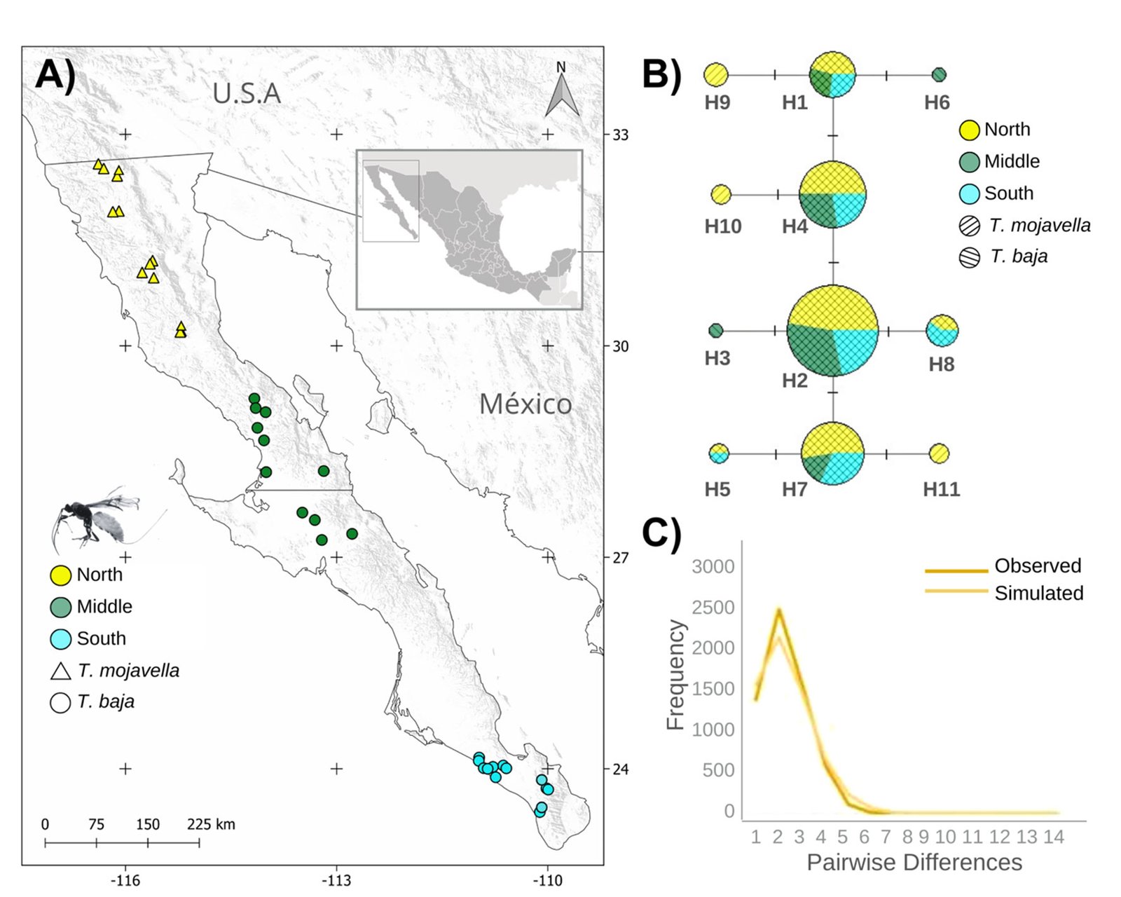
Figure 1. A, Localities sampled of Digonogastra sp. in the Baja California Peninsula. The geographical distribution is marked using colors and the host moth species is indicated whit shapes; B, haplotype network. The geographical distribution is marked using colors and the host moth species with lines; C, graph depicting the observed and simulated distribution of paired sequence differences.

Figure 2. The genera of parasitoid wasps sampled from yucca fruits in the Baja California Peninsula. On the upper side is the genus Digonogastra; on the bottom is Bassus.
DNA extraction and molecular marker amplification. We extracted DNA from 119 wasps using the commercial Qiagen DNeasy Blood & Tissue Kit. The sample consisted of 114 adult individuals and 5 in the pupal stage. A fragment of the Cytochrome Oxidase subunit I (COI) marker was amplified via PCR using the universal primers for invertebrates described by Folmer et al. (1994); LCO1490 (5’-GGTCAACAAATCATAAAGATATTGG-3’) and HCO2198 (5’-TAAACTTCAGGGTG ACCAAAAAATCA-3’). The PCR mixture included 5 µl of Buffer (1x), 1.5 µl of MgCL (2.5mM), 0.3 µl of dNTPs (0.16mM), 0.6 µl of each primer at 10 µM, 0.2 µl of Taq polymerase (1 unit), 1 µl of DNA, and 5.8 µl of molecular-grade water, resulting in a 15 µl reaction volume.
The thermal cycler was set up with the following conditions: an initial denaturation at 94 ºC for 5 min, followed by 35 cycles of denaturation at 94 ºC for 1 min, annealing at 50 ºC for 1 min, and extension at 68 ºC for 1 min. A final elongation step was performed at 72 ºC for 5 min. Amplification quality was confirmed using 1% agarose gel electrophoresis. The PCR products were sequenced by SeqXcel (www.seqxcel.com) for further analysis.
Genetic diversity and population genetic structure. The sequences were visualized, aligned, and edited using the BioEdit software (Hall, 1999). Sequences from individuals identified morphologically were submitted to BLAST to confirm the parasitoid genus (Blast.ncbi.nlm.nih.gov). The sample size of Digonogastra sp. (N = 111) allowed for diversity and population structure analysis. The genetic diversity of Digonogastra species was assessed using DNAsp software (Rozas et al., 2003). This involved calculating the number of haplotypes, haplotype diversity, and nucleotide diversity (Nei & Li, 1979; Nei, 1987). To investigate the genealogical relationships among the identified haplotypes, we constructed a haplotype network using the Median-Joining method in NETWORK 5.0 software (Bandelt et al., 1999). We constructed a phylogenetic tree using the haplotypes obtained for Digonogastra sp. to determine whether the detected diversity in the Baja California Peninsula is unique to this region or present elsewhere. We included sequences available in the NCBI from Canada. The genera Alabagrus (Sharkey & Chapman, Unpublished; GenBank: MF361682.1) and Cotesia (Hebert et al., 2016) were employed as outgroups. The tree was constructed using the Maximum Likelihood method, with 1000 bootstrap replicates and the HKY+I substitution model, which showed the best fit to the data (highest AIC value), as determined by the jModelTest program (Darriba et al., 2012).
To assess genetic differentiation of Digonogastra spp. across its geographical distribution in the peninsula, we conducted 3 Molecular Variance Analyses (AMOVA). First, we examined how geographical distances affected the distribution of genetic diversity. We divided the data into 3 categories based on their location in the peninsula: north, center, and south (Fig. 1A). Then, we assessed whether genetic differentiation was due to environmental factors, grouping the data based on their ecoregion of origin. We based our categorization on the ecoregions proposed by Gonzales-Abraham et al. (2010). Lastly, our third analysis examined whether genetic differentiation was related to the host, grouping the data based on the host moths, T. mojavella and T. baja. The ARLEQUIN software (Excoffier et al., 2005) was employed for these analyses.
We evaluated historical demographic changes in the wasp population using the pairwise sequence differences distribution analysis (mismatch analysis) performed in the ARLEQUIN software. The shape of the mismatch distribution is used to infer whether a population expansion has occurred (Rogers & Harpending, 1992). A unimodal distribution indicates population expansion, while a multimodal distribution suggests a stable population size. Additionally, the sum of squared deviations (SSD) is employed to validate the expansion model (Navascués et al., 2006). A significant SSD (p < 0.05) rejects the population expansion model.
Phenotypic variation. Phenotypic variation of the parasitoid wasps was evaluated by measuring 106 adult
individuals of the Digonogastra genus (excluding individuals in the pupal stage). No morphometric analyses were conducted for Bassus specimens due to their small sample size (N = 8). Measurements of the 106 adults were conducted with Infinity Analyze software (Lumenera, Canadá), calibrated in millimeters and verified with a conventional ruler. We measured 18 external morphological characters of the adult individuals (Table 1). Measurements were taken on the left side of the individuals and included the length from the head to the end of the last metasoma segment, the scape width, antenna length, mesosoma (thorax) and metasoma (abdomen) width and length, femur width, total leg length, anterior wing length, and the length of 5 wing vein components: C+SC+R, 1RS, (RS+M)a, 2RS, and r-rs. For females, we also measured the length and width of the ovipositor and the length of the ovipositor apex (Table 1). We calculated the mean, standard deviation, and coefficient of variation of each measured character. A correlation matrix was created using the Pearson Correlation Coefficient (r) between pairs of characters, determining the significance values (p) for each correlation. All morphometric measurements were analyzed with JMP 5.01 software (SAS Cary, New Jersey, USA).
We assessed 3 potential sources of variation for the phenotypic differentiation among parasitoid wasps in the Baja California Peninsula: sexual dimorphism, the ecoregions in which they are distributed, and the host species of Tegeticula moths. We conducted a Multivariate Analysis of Variance (MANOVA) for each factor using all measured characters. We also performed an Analysis of Variance (ANOVA) to determine which trait contributes significantly to phenotypic differences. Each wasp was assigned to an ecoregion based on its geographical origin (Gonzales-Abraham et al., 2010). The wasps were found in 6 ecoregions: Sierra Juárez, Sierra San Pedro Mártir, Chaparral, Central Desert, Magdalena Plains, and Cape Lowland Forest.
Results
We collected a total of 119 parasitoid wasps from 35 locations across the Baja California Peninsula (Fig. 1A, Table S1). Two genera of parasitoid wasps belonging to the Braconidae family were collected: Bassus and Digonogastra. Eight female individuals of Bassus sp. (6.7%) emerged from fruits in 2 different locations. Seven Bassus specimens were collected in Y. valida fruits, while 1 emerged from Y. capensis. All these fruits contained T. baja larvae. In contrast, we collected 111 Digonogastra individuals (93.3%), with 68 males and 38 females from 33 different sites across 32.58° to 23.38° N latitude. Out of these, 57 individuals of Digonogastra sp. emerged from Y. schidigera fruits where T. mojavella was also found. The remaining 54 individuals were found in Y. valida, Y. valida x Y. capensis, and Y. capensis fruits, where T. baja larvae were also present.
Table 1
Mean (M), standard deviation (SD), and coefficient of variation in percentage (CV) of the evaluated morphological traits in female and male individuals of Digonogastra sp. in the Baja California Peninsula. The results of the analysis of variance (ANOVA) performed for sexual dimorphism (S), ecoregions (E), and host (H) are presented with significance levels denoted as follows: p > 0.05 (ns), p < 0.05 (*), and p < 0.0001 (***).
| Trait | Female | Male | ANOVA | ||||||
| M | SD | CV | M | SD | CV | S | E | H | |
| Body length: | 9.03 | 1.29 | 14.24 | 7.34 | 1.47 | 20.04 | *** | * | ns |
| Antenna: | |||||||||
| Total length | 6.88 | 0.73 | 10.58 | 6.16 | 1.08 | 17.52 | *** | * | ns |
| Escapo width | 0.24 | 0.03 | 12.61 | 0.19 | 0.04 | 22.92 | *** | ns | ns |
| Leg: | |||||||||
| Total length | 6.97 | 0.90 | 12.96 | 5.21 | 1.08 | 20.67 | *** | * | ns |
| Femur width | 0.52 | 0.06 | 12.23 | 0.36 | 0.08 | 22.93 | *** | * | ns |
| Mesosoma: | |||||||||
| Lateral width | 2.17 | 0.32 | 14.54 | 1.61 | 0.34 | 21.11 | *** | ns | ns |
| Lateral length | 3.17 | 0.45 | 14.08 | 2.46 | 0.58 | 23.59 | *** | * | ns |
| Metasoma: | |||||||||
| Lateral width | 2.14 | 0.56 | 26.32 | 1.33 | 0.44 | 33.15 | *** | * | ns |
| Lateral length | 4.84 | 0.81 | 16.83 | 4.03 | 0.86 | 21.20 | *** | * | ns |
| Wing: | |||||||||
| Total length | 8.47 | 0.95 | 11.19 | 6.30 | 1.26 | 19.96 | *** | * | ns |
| C+SC+R length | 3.99 | 0.48 | 12.14 | 3.03 | 0.62 | 20.62 | *** | * | ns |
| 1RS length | 0.26 | 0.04 | 15.15 | 0.21 | 0.05 | 23.26 | *** | ns | ns |
| (RS+M)a length | 1.00 | 0.13 | 12.46 | 0.70 | 0.15 | 21.33 | *** | * | ns |
| 2RS length | 0.69 | 0.10 | 13.98 | 0.51 | 0.10 | 18.78 | *** | * | ns |
| r-rs length | 0.29 | 0.05 | 17.53 | 0.21 | 0.05 | 21.47 | *** | * | ns |
| Ovipositor: | |||||||||
| Total length | 8.37 | 1.07 | 12.84 | NA | NA | NA | NA | ns | ns |
| Lateral width | 0.06 | 0.01 | 10.54 | NA | NA | NA | NA | ns | ns |
| Apex length | 0.36 | 0.05 | 14.22 | NA | NA | NA | NA | ns | ns |
Genetic diversity and population genetic structure. We obtained a 632 bp sequence for each of the 8 individuals of Bassus sp. These sequences did not exhibit site variability, defining them as a single haplotype. Further analyses were not conducted due to the lack of variation. Compared to NCBI sequences, they showed 97% coverage, an E-value of 0.0, and 97.73% identity with the genus Bassus.
The alignment of the 111 Digonogastra wasps allows us to obtain 563 bp and reveals 7 variable sites. We obtained 100% coverage, 0.0 E-value, and 93.61% identity compared with NCBI sequences. Nucleotide diversity (Pi) for Digonogastra sp. in the peninsula was 0.00228, and haplotype diversity (Hd) was 0.775. The 7 variable sites defined 11 haplotypes. Haplotype 2 was most abundant, followed by haplotypes 4, 7, and 1 (Fig. 1B). Six of the 11 haplotypes were found throughout the entire geographic range, 3 were unique to the northern region, and 2 were only found in the central part of the peninsula. The phylogenetic analysis revealed that 11 haplotypes from the peninsula formed a single clade with 100% support (Fig. S1). This clade was separated from 5 clades found in Canada, although with low bootstrap support (43%).

Figure 3. Mean and standard deviation of 5 significantly different traits of Digonogastra sp. among Baja California Peninsula ecoregions. From north to south, they are listed as follows: Sierra Juárez (SJ), Sierra San Pedro Mártir (SSPM), Chaparral (Ch), Central Desert (DC), Magdalena Plains (PM), and Cape Region (CR). Individuals with larger sizes are marked in red, while those with smaller sizes are marked in blue.
The geographical distance did not cause genetic differentiation in Digonogastra sp. individuals (Fst = -0.01319, S.S. = 41.176, p = 0.84360 ± 0.01326). Similarly, no differentiation was found between individuals inhabiting different ecoregions (Fst = -0.01838, S.S. = 38.933, p = 0.05181 ± 0.00599) and individuals parasitizing different host species (Fst = 0.01877, S.S. = 41.853, p = 0.06158 ± 0.00750). Considering that Digonogastra sp. individuals from the peninsula form a single genetic clade, we performed a demographic analysis (i.e., mismatch analysis), including all individuals as a single population. The distribution of paired differences was unimodal, and the SSD test did not reject the expansion hypothesis (p = 0.09).
Phenotypic variation. Digonogastra sp. females had an average body length of 9.03 mm, with their morphological characters showing coefficients of variation between 10% and 27%. Males had an average body length of 7.34 mm, with morphological characters exhibiting coefficients of variation between 17% and 33%. The most variable character was the metasoma width for females and males, with coefficients of variation of 26.32% and 33.15%, respectively. Females exhibited significant correlations between all analyzed traits (r² > 0.6; p < 0.05), except for ovipositor width, ovipositor tip length, and scape width (r² < 0.3; p > 0.05), while males showed significant correlations across all traits (Fig. S2).
Morphological differences between males and females were significant (F test = 5.21, F = 25.74, p < 0.0001), with females being consistently larger in all measured characters (Table 1). Similarly, significant differences were found among individuals from different ecoregions (Wilks’ Lambda = 0.195, F = 1.83, p < 0.0002; Table 1, Fig. 3), with 11 out of 18 characters showing high variation (Table 1). Finally, significant differences observed in the MANOVA (F test = 0.40, F = 1.98, p < 0.027) indicate that the traits of the wasps vary according to the host groups, even though the ANOVA did not detect significant differences in individual traits (Table 1).
Discussion
The taxonomic, genetic, and phenotypic diversity of parasitoid wasps is influenced by environmental and spatial distribution of their populations and hosts (Althoff & Thompson, 2001; Baer et al., 2004; Harrison et al., 2022). Here, we have recorded for the first time Bassus wasps attacking Tegeticula moths. Additionally, we include the first report of a Digonogastra wasps attacking T. baja. The 111 Digonogastra sp. individuals from various environments showed low genetic diversity across the peninsula, suggesting a single panmictic population that had experienced historical demographic expansion. We also identified sexual dimorphism and morphometric variation due to ecoregions and diferent host.
Genetic diversity estimates for Digonogastra sp. in the Baja California Peninsula are moderate (N = 111, 11 haplotypes, Hd = 0.77, pi = 0.00228). Similar genetic diversity values have been reported for other parasitoid wasps in the Braconidae family (Baer et al., 2004; Hufbauer et al., 2004). For Digonogastra sp., we obtained values of reduced nucleotide diversity alongside high haplotype diversity, indicating that population haplotypes are very similar to each other, as shown in our haplotype network (Fig. 1B). This pattern is observed in species that have experienced population expansion events (Roderick, 1996). Individuals from the Baja California Peninsula have different haplotypes than those recorded to the north of the genus’s distribution, and they cluster into a different clade from the haplotypes reported in Canada (Fig. S1). Future sampling in intermediate areas will help determine whether the diversity found in this study is shared with other zones of their distribution or is restricted to this geographic region.
We found no genetic diversity structuring Digo-
nogastra sp. individuals from different geographic areas, ecoregions, or hosts (i.e., Tegeticula spp.) in the Baja California Peninsula. Furthermore, Digonogastra individuals share most of the recorded haplotypes, suggesting a single panmictic population. A similar pattern was observed in the parasitoid wasp Eusandalum sp., which attacked 11 species of Prodoxus spp. moths in a Yucca complex, in the USA (Althoff, 2008). These 2 wasp genera are known for their generalist nature, which may be related to the genetic differentiation pattern across the landscape. Eusandalum sp., in particular, can lay eggs throughout the year and parasitize any available Prodoxus species, which helps to maintain a continuous population across the landscape (Althoff, 2008). Digonogastra has been recorded attacking various Tegeticula and Prodoxus moths (Force & Thompson, 1984), also present in the peninsula (obs. pers; Althoff et al., 2007). Therefore, other potential food sources could contribute to the population connectivity of Digonogastra sp. throughout its distribution. For example, Prodoxus larvae have been observed as a year-round resource (Powell, 1989). However, further studies are needed to confirm the presence of Digonogastra sp. attacking other Tegeticula and Prodoxus species in this region.
The panmictic population of Digonogastra sp. in the Baja California Peninsula exhibited a historical population expansion, as supported by different analyses (Fig. 1C). The close parasitoid-host interaction with Yucca-pollinating moths implies that demographic changes in their hosts (moths) and in the plants can directly affect the demographics of their populations. Previous studies have recorded the influence of glacial and interglacial cycles in the Quaternary on the demographic history of organisms in the Baja California Peninsula (Garrick et al., 2009; Harrington et al., 2018; Nason et al., 2002). Demographic changes have been documented for the 3 Yucca species in this region, and their habitat has expanded since the last interglacial maximum (Alemán et al., 2024; Arteaga et al., 2020; De la Rosa et al., 2020). Since Digonogastra sp. individuals rely on Yucca plant fruits to complete their life cycle, as these fruits host the moth larvae that serve as their food source, the population expansion found in these wasps may be a consequence of the population expansion observed in the plants that host their hosts.
Phenotypic variability and sexual dimorphism of Digonogastra sp. Geographic variation in phenotype is a common factor in insect populations (Stilwell & Fox, 2007, 2009). The spatial structure of this variation can be determined by environmental conditions, genetic composition, and/or ecological interactions (Agrawal, 2001; Resh & Cardé, 2009; Seifert et al., 2022). For Digonogastra sp. in the Baja California Peninsula, our results show phenotypic variability and a high phenotypic correlation among the studied traits (Table 1, Fig. S2). However, the female ovipositor showed low variation and correlation with the other traits, indicating that its variation did not depend closely on the expression of other traits. Females use the ovipositor to pierce the fruit pericarp, access the moth larvae, and lay eggs (Crabb & Pellmyr, 2006; Resh & Cardé, 2009; Vilhelmsen et al., 2001). The function of this trait is closely related to its fitness, as the arrangement of wasp eggs near moth larvae inside the fruit determines their survival by allowing access to their food source. This may favor reduced variation in ovipositor size (Mazer & Damuth, 2001; Pigliucci, 2003).
Like other parasitoid wasps, Digonogastra sp. exhibits sexual dimorphism (Hurlbutt, 1987; Quicke, 2015), with females being larger in all the traits assessed compared to males (Table 1). Sexual dimorphism in Hymenoptera is partly attributed to complementary sex determination (CSD), where fertilized eggs develop into females and unfertilized eggs into males (Quicke, 2015; Resh & Cardé, 2009). Studies on parasitoid wasps have shown that females typically allocate more resources to fertilized eggs (females) than unfertilized ones (males; Ellers & Jervis, 2003; Jervis et al., 2008; Quicke, 2015; Resh & Cardé, 2009; Visser, 1994). Therefore, the variation in size can be explained by the interplay between CSD and the differential allocation of resources during oviposition.
The environmental heterogeneity in which these wasps are distributed in the Baja California Peninsula also affects their phenotypic variation (Fig. 3). Similar patterns have been observed in butterflies, where species distributed across a broad environmental range exhibit greater variation in organism size compared to species with a more restricted environmental distribution (Seifert et al., 2022). The relationship between body size and environmental variability is attributed to the significant influence of the environment on the development and growth of holometabolous insects, considering factors such as temperature, humidity, and nutrition (Davidowitz et al., 2004; Stillwell & Fox, 2007; Wonglersak et al., 2020). Digonogastra sp. wasps from the Baja California Peninsula occur in different ecosystems, including mountainous areas, deserts, and lowland forests, with variable climatic conditions. However, this study did not investigate the environmental factors that may affect morphological differentiation, which is a topic for future research.
Ecological interactions between plants, herbivores, and parasitoids are significant drivers of biological diversity in terrestrial ecosystems (Schoonhoven et al., 2005). The phenotypic variation in Digonogastra sp. is influenced by the interaction between the wasp, the ecoregion and the host. Tritrophic interactions have shown that a favorable environment for plant growth leads to better nutrition for herbivorous insects, enhancing the development and performance of parasitoids (Han et al., 2019; Pekas & Wäckers, 2020; Schoonhoven et al., 2005). These “bottom-up” cascades have been studied and have shown that the nutritional quality of the plant and the host insect plays a critical role in parasitoids. For instance, it has been observed that parasitoid wasps have increased fitness when they inhabit more fertile soils (Pekas & Wäckers, 2020; Sarfraz et al., 2009). This suggests that the different trophic levels may influence the phenotypic diversity of this wasp, namely the plant and herbivore.
In conclusion, our study records for the first time the genus of parasitoid wasps Bassus attacking Tegeticula moths and increases the diversity of hosts attacked by Digonogastra wasps. The genetic diversity of Digonogastra sp. in the Baja California Peninsula is moderate, forming a single panmictic population with signs of historical demographic expansion. Phenotypic variation is influenced by sexual dimorphism, ecoregions, and their host, this highlights the various factors that can shape the phenotype of these parasitoid wasps. The presence of Digonogastra sp. in different ecoregions suggests the influence of ecological interactions on their phenotypic diversity.
Acknowledgements
The authors are grateful to Leonardo de la Rosa, Mario Salazar, José Delgadillo, and Darlene van der Heiden for their help with laboratory analysis, technical support, and assistance in the fieldwork. C.R.A.H thanks the Centro de Investigación Científica y Educación Superior de Ensenada (CICESE) and Universidad Autónoma de Baja California (UABC) for offering academic support. This study was supported financially by Consejo Nacional de Ciencia y Tecnología (Conacyt) (CB-2014-01-238843, infra-2014-1-226339). The Rufford Foundation also provided financial support for a part of this study (RSG 13704-1) and the Jiji Foundation. The authors thank the Associate Editor and the anonymous reviewer for their valuable comments. The authors do not have any conflict of interest to declare.
Haplotypes from this study were deposited in the GenBank with accession numbers PQ252653-PQ252665.
References
Abdala-Roberts, L., Puentes, A., Finke, D. L., Marquis, R. J., Montserrat, M., Poelman, E. H. et al. (2019). Tri-trophic interactions: bridging species, communities and ecosystems. Ecology Letters, 22, 2151–2167. https://doi.org/10.1111/ele.13392
Agrawal, A. A. (2001). Phenotypic plasticity in the interactions and evolution of species. Science, 294, 321–326. https://doi.org/10.1126/science.1060701
Althoff, D. M., & Thompson, J. N. (2001). Geographic structure in the searching behaviour of a specialist parasitoid: combining molecular and behavioural approaches. Journal of Evolutionary Biology, 14, 406–417. https://doi.org/10.1046/j.1420-9101.2001.00286.x
Althoff, D. M., Svensson, G. P., & Pellmyr, O. (2007). The influence of interaction type and feeding location on the phylogeographic structure of the yucca moth community associated with Hesperoyucca whipplei. Molecular Phy-
logenetics and Evolution, 43, 398–406. https://doi.org/10.
1016/j.ympev.2006.10.015
Althoff, D. M. (2008). A test of host-associated differentiation across the ‘parasite continuum’in the tri-trophic interaction among yuccas, bogus yucca moths, and parasitoids. Molecular Ecology, 17, 3917–3927. https://doi.org/10.1111/j.1365-294X.2008.03874.x
Althoff, D. M., Segraves, K. A., Smith, C. I., Leebens-Mack, J., & Pellmyr, O. (2012). Geographic isolation trumps coevolution as a driver of yucca and yucca moth diversification. Molecular Phylogenetics and Evolution, 62, 898–906. https://doi.org/10.1016/j.ympev.2011.11.024
Althoff, D. M., & Segraves, K. A. (2022). Evolution of antag-
onistic and mutualistic traits in the yucca-yucca moth obligate pollination mutualism. Journal of Evolutionary Biology, 35, 100–108. https://doi.org/10.1111/jeb.13967
Arteaga, M. C., Bello-Bedoy, R., & Gasca-Pineda, J. (2020). Hybridization between yuccas from Baja California: Genomic and environmental patterns. Frontiers in Plant Science, 11, 685. https://doi.org/10.3389/fpls.2020.00685
Baer, C. F., Tripp, D. W., Bjorksten, T. A., & Antolin, M. F. (2004). Phylogeography of a parasitoid wasp (Diaeretiella rap-
ae): no evidence of host-associated lineages. Molecular Ecology, 13, 1859–1869. https://doi.org/10.1111/j.1365-294X.
2004.02196.x
Bandelt, H. J., Forster, P., & Röhl, A. (1999). Median-joining networks for inferring intraspecific phylogenies. Molecular Biology and Evolution, 16, 37–48. https://doi.org/10.1093/oxfordjournals.molbev.a026036
Carmona, D., Fitzpatrick, C. R., & Johnson, M. T. (2015). Fifty years of co-evolution and beyond: integrating co-evolution from molecules to species. Molecular Ecology, 24, 5315–5329. https://doi.org/10.1111/mec.13389
Crabb, B. A., & Pellmyr, O. (2006). Impact of the third trophic level in an obligate mutualism: do yucca plants benefit from parasitoids of yucca moths? International Journal of Plant Sciences, 167, 119–124. https://doi.org/10.1086/497844
Cuautle, M., & Rico-Gray, V. (2003). The effect of wasps and ants on the reproductive success of the extrafloral nectaried plant Turnera ulmifolia (Turneraceae). Functional Ecology, 17, 417–423. https://doi.org/10.1046/j.1365-2435.2003.00732.x
Darriba, D., Taboada, G. L., Doallo, R., & Posada, D. (2012). jModelTest 2: more models, new heuristics and parallel computing. Nature Methods, 9, 772. https://doi.org/10.1038/nmeth.2109
Davidowitz, G., D’Amico, L. J., & Nijhout, H. F. (2004). The effects of environmental variation on a mechanism that controls insect body size. Evolutionary Ecology Research, 6, 49–62.
De la Rosa-Conroy, L., Gasca-Pineda, J., Bello-Bedoy, R., Eguiarte, L. E., & Arteaga, M. C. (2020). Genetic patterns and changes in availability of suitable habitat support a colonization history of a North American perennial plant. Plant Biology, 22, 233–242. https://doi.org/10.1111/plb.13053
Ellers, J., & Jervis, M. (2003). Body size and the timing of egg production in parasitoid wasps. Oikos, 102, 164–172. https://doi.org/10.1034/j.1600-0706.2003.12285.x
Engelmann, G. (1872). The flower of yucca and its fertilization. Bulletin of the Torrey Botanical Club, 3, 33–33.
Excoffier, L., Laval, G., & Schneider, S. (2005). Arlequin (version 3.0): an integrated software package for population genetics data analysis. Evolutionary Bioinformatics Online, 2005,47–50. https://doi.org/10.1177/117693430500100003
Folmer, O., Hoeh, W. R., Black, M. B., & Vrijenhoek, R. C. (1994). Conserved primers for PCR amplification of mitochondrial DNA from different invertebrate phyla. Molecular Marine Biology and Biotechnology, 3, 294–299.
Force, D. C., & Thompson, M. L. (1984). Parasitoids of the immature stages of several southwestern yucca moths. The Southwestern Naturalist, 29, 45–56. https://doi.org/
10.2307/3670768
Garrick, R. C., Nason, J. D., Meadows, C. A., & Dyer, R. J. (2009). Not just vicariance: phylogeography of a Sonoran Desert euphorb indicates a major role of range expansion along the Baja peninsula. Molecular Ecology, 18, 1916–1931. https://doi.org/10.1111/j.1365-294X.2009.04148.x
Godfray, H. C. J. (1994). Parasitoids: behavioral and evolut-
ionary ecology. New Jersey: Princeton University Press.
González-Abraham, C. E., Garcillán, P. P., & Ezcurra, E. (2010). Ecorregiones de la península de Baja California: una síntesis. Boletín de la Sociedad Botánica de México, 87, 69–82. https://doi:10.17129/botsci.302
Hall, T. A. (1999). BioEdit: a user-friendly biological sequence alignment editor and analysis program for Windows 95/98/NT. Nucleic Acids Symposium Series, 41,95–98.
Han, P., Desneux, N., Becker, C., Larbat, R., Le Bot, J., Adamowicz, S. et al. (2019). Bottom-up effects of irrigation, fertilization and plant resistance on Tuta absoluta: implications for Integrated Pest Management. Journal of Pest Science, 92, 1359–1370. https://doi.org/10.1007/s10340-018-1066-x
Harrington, S. M., Hollingsworth, B. D., Higham, T. E., & Reeder, T. W. (2018). Pleistocene climatic fluctuations drive isolation and secondary contact in the red diamond rattlesnake (Crotalus ruber) in Baja California. Journal of Biogeography, 45, 64–75. https://doi.org/10.1111/jbi.13114
Harrison, K., Tarone, A. M., DeWitt, T., & Medina, R. F. (2022). Predicting the occurrence of host-associated differentiation in parasitic arthropods: a quantitative literature review. Entomologia Experimentalis et Applicata, 170, 5–22. https://doi.org/10.1111/eea.13123
Hebert, P. D., Ratnasingham, S., Zakharov, E. V., Telfer, A. C., Levesque-Beaudin, V., Milton, M. A. et al. (2016). Counting animal species with DNA barcodes: Canadian insects. Philosophical Transactions of the Royal Society B: Biological Sciences, 371, 20150333. https://doi.org/10.1098/rstb.2015.0333
Heil, M. (2008). Indirect defence via tritrophic interactions.
New Phytologist, 178, 41–61. https://doi.org/10.1111/j.1469-
8137.2007.02330.x
Hufbauer, R. A., Bogdanowicz, S. M., & Harrison, R. G. (2004). The population genetics of a biological control introduction: mitochondrial DNA and microsatellie variation in native and introduced populations of Aphidus ervi, a parisitoid wasp. Molecular Ecology, 13, 337–348. https://doi.org/10.
1046/j.1365-294X.2003.02084.x
Hurlbutt, B. (1987). Sexual size dimorphism in parasitoid wasps. Biological Journal of the Linnean Society, 30, 63–89. https://doi.org/10.1111/j.1095-8312.1987.tb00290.x
Jervis, M. A., Ellers, J., & Harvey, J. A. (2008). Resource acquisition, allocation, and utilization in parasitoid reproductive strategies. Annual Review of Entomology, 53,361–385. https://doi.org/10.1146/annurev.ento.53.103106.093
433
Kankare, M., Van Nouhuys, S., & Hanski, I. (2005). Genetic divergence among host-specific cryptic species in Cotesia melitaearum aggregate (Hymenoptera: Braconidae), parasitoids of checkerspot butterflies. Annals of the Entomological Society of America, 98, 382–394. https://doi.org/10.1603/0013-8746(2005)098[0382:GDAHCS]2.0.CO;2
Kappers, I. F., Hoogerbrugge, H., Bouwmeester, H. J., & Dicke, M. (2011). Variation in herbivory-induced volatiles among cucumber (Cucumis sativus L.) varieties has consequences for the attraction of carnivorous natural enemies. Journal of Chemical Ecology, 37, 150–160. https://doi.org/10.1007/s10886-011-9906-7
Karns, G. (2009). Genetic differentiation of the parasitoid, Cotesia congregata (Say), based on host-plant complex (M. Sc. Thesis). Virginia Commonwealth University. VA, USA. https://doi.org/10.25772/1E5V-N037
Lenz, L. W. (1998). Yucca capensis (Agavaceae, Yuccoideae), a new species from Baja California Sur, Mexico. Cactus and Succulent Journal, 70, 289–296.
Lozier, J. D., Roderick, G. K., & Mills, N. J. (2009). Molecular markers reveal strong geographic, but not host associated, genetic differentiation in Aphidius transcaspicus, a parasitoid of the aphid genus Hyalopterus. Bulletin of Entomological Research, 99, 83–96. https://doi.org/10.1017/S0007485308006147
Mazer, S. J., & Damuth, J. (2001). Nature and causes of variation. In C. W. Fox, D. A. Roff, & D. J. Fairbairn (Ed). Evolutionary ecology: concepts and case studies (pp. 3–15). Oxford, UK: Oxford University Press.
Nason, J. D., Hamrick, J. L., & Fleming, T. H. (2002). Historical vicariance and postglacial colonization effects on the evolution of genetic structure in Lophocereus, a Sonoran Desert columnar cactus. Evolution, 56, 2214–2226. https://doi.org/10.1111/j.0014-3820.2002.tb00146.x
Navascués, M., Vaxevanidou, Z., González-Martínez, S. C., Climent, J., Gil, L., & Emerson, B. C. (2006). Chloroplast microsatellites reveal colonization and meta-
population dynamics in the Canary Island pine. Molecular Ecology, 15, 2691–2698. https://doi.org/10.1111/
j.1365-294X.2006.02960.x
Nei, M., & Li, W. H. (1979). Mathematical model for studying genetic variation in terms of restriction endonucleases. Proceedings of the National Academy of Sciences, 76, 5269–5273. https://doi.org/10.1073/pnas.76.10.5269
Nei, M. (1987). Molecular evolutionary genetics. New York: Columbia University Press.
Pekas, A., & Wäckers, F. L. (2020). Bottom-up effects on tri-trophic interactions: Plant fertilization enhances the fitness of a primary parasitoid mediated by its herbivore host. Journal of Economic Entomology, 113, 2619–2626. https://doi.org/10.1093/jee/toaa204
Pellmyr, O., & Leebens-Mack, J. (1999). Forty million years of mutualism: evidence for Eocene origin of the yucca-yucca moth association. Proceedings of the National Academy of Sciences, 96, 9178–9183. https://doi.org/10.1073/pnas.96.
16.9178
Pellmyr, O. (2003). Yuccas, yucca moths, and coevolution: a review. Annals of the Missouri Botanical Garden, 90, 35–55. https://doi.org/10.2307/3298524
Pigliucci, M. (2003). Phenotypic integration: studying the ecology and evolution of complex phenotypes. Ecology Letters, 6, 265–272. https://doi.org/10.1046/j.1461-0248.2003.00428.x
Powell, J. A. (1989). Synchronized, mass-emergences of a yucca moth, Prodoxus Y-inversus (Lepidoptera: Prodoxidae), after 16 and 17 years in diapause. Oecologia, 81, 490–493. https://doi.org/10.1007/BF00378957
Quicke, D. L. (2015). The Braconid and Ichneumonid parasitoid wasps: Biology, Systematics, Evolution and Ecology. Metopiinae. Oxford: Wiley Blackwell.
Resh, V. H., & Cardé, R. T. (Eds.). (2009). Encyclopedia of insects. San Diego, CA: Academic press.
Roderick, G. K. (1996). Geographic structure of insect populations: gene flow, phylogeography, and their uses. Annual Review of Entomology, 41, 325–352. https://doi.org/10.1146/annurev.en.41.010196.001545
Rogers, A. R., & Harpending, H. (1992). Population growth makes waves in the distribution of pairwise genetic differences. Molecular Biology and Evolution, 9, 552–569. https://doi.org/10.1093/oxfordjournals.molbev.a040727
Rozas, J., Sánchez-DelBarrio, J. C., Messeguer, X., & Rozas, R. (2003). DnaSP, DNA polymorphism analyses by the coalescent and other methods. Bioinformatics, 19, 2496–2497. https://doi.org/10.1093/bioinformatics/btg359
Sánchez, J. A., Romero, J., Ramírez, S., Anaya, S., & Carrillo, J. L. (1998). Géneros de Braconidae del estado de Guanajuato (Insecta: Hymenoptera). Acta Zoológica Mexicana (nueva serie), 79, 59–137. https://doi.org/10.21829/azm.1998.74741721
Sarfraz, M., Dosdall, L. M., & Keddie, B. A. (2009). Host plant nutritional quality affects the performance of the parasitoid Diadegma insulare. Biological Control, 51, 34–41. https://doi.org/10.1016/j.biocontrol.2009.07.004
Schoonhoven, L. M., Van Loon, J. J., & Dicke, M. (2005). Insect-plant biology. Oxford: Oxford University Press.
Seifert, C. L., Strutzenberger, P., & Fiedler, K. (2022). Ecological specialisation and range size determine intraspecific body size variation in a speciose clade of insect herbivores. Oikos, 2022, e09338. https://doi.org/10.1111/oik.09338
Singer, M. S., & Stireman III, J. O. (2005). The tri-trophic niche concept and adaptive radiation of phytophagous insects. Ecology Letters, 8, 1247–1255. https://doi.org/10.
1111/j.1461-0248.2005.00835.x
Stillwell, R. C., & Fox, C. W. (2007). Environmental effects on sexual size dimorphism of a seed-feeding beetle. Oecologia, 153, 273–280. https://doi.org/10.1007/s00442-007-0724-0
Stillwell, R. C., & Fox, C. W. (2009). Geographic variation in body size, sexual size dimorphism and fitness components of a seed beetle: local adaptation versus phenotypic plasticity. Oikos, 118, 703–712. https://doi.org/10.1111/j.1600-0706.2008.17327.x
StiremanIII, J. O., Nason, J. D., & Heard, S. B. (2005). Host-associated genetic differentiation in phytophagous insects: general phenomenon or isolated exceptions? Evidence from a goldenrod-insect community. Evolution, 59, 2573–2587. https://doi.org/10.1111/j.0014-3820.2005.tb00970.x
Takabayashi, J., & Dicke, M. (1996). Plant-carnivore mutualism through herbivore-induced carnivore attractants. Trends
in plant science, 1, 109–113. https://doi.org/10.1016/S1360-
1385(96)90004-7
Tamura, K., Dudley, J., Nei, M., & Kumar, S. (2007). MEGA4: molecular evolutionary genetics analysis (MEGA) software version 4.0. Molecular Biology and Evolution, 24, 1596–1599. https://doi.org/10.1093/molbev/msm092
Turner, R. M., Bowers, J. E., & Brugess, T. L. (2022). Sonoran Desert plants: an ecological atlas. Tucson: University of Arizona Press.
Vilhelmsen, L., Isidoro, N., Romani, R., Basibuyuk, H. H., & Quicke, D. L. (2001). Host location and oviposition in a basal group of parasitic wasps: the subgenual organ, ovipositor apparatus and associated structures in the Orussidae (Hymenoptera, Insecta). Zoomorphology, 121, 63–84. https://doi.org/10.1007/s004350100046
Visser, M. E. (1994). The importance of being large: the relationship between size and fitness in females of the parasitoid Aphaereta minuta (Hymenoptera: Braconidae). Journal of Animal Ecology, 63, 963–978. https://doi.org/10.
2307/5273
Wonglersak, R., Fenberg, P. B., Langdon, P. G., Brooks, S. J., & Price, B. W. (2020). Temperature-body size responses in insects: a case study of British Odonata. Ecological Entomology, 45, 795–805. https://doi.org/10.1111/een.12853

Diversity of anurans and use of microhabitatsin three vegetation coverages of the Santuario de Flora y Fauna Los Colorados, Colombian Caribbean
Omer José Jiménez-Ortega a, d, Keiner L. Tílvez b, Joselin Castro-Palacios a,
Andrés García c, *, Gabriel R. Navas a, Julio Abad Ferrer-Sotelo e, Dilia Naranjo-Calderón e, Juan Gabriel Díaz-Castellar e, Víctor Buelvas-Meléndez e
a Universidad de Cartagena, Campus San Pablo, Grupo de Investigación en Hidrobiología, Programa de Biología, Carrera 50#24-120, Zaragocilla, Cartagena de Indias, Colombia.
b Universidad de Cartagena, Campus San Pablo, Grupo de Investigación en Biología Descriptiva y Aplicada, Carrera 50#24-120, Zaragocilla, Cartagena de Indias, Colombia
c Universidad Nacional Autónoma de México, Instituto de Biología, Estación de Biología Chamela, Apartado postal 21, 48980 San Patricio, Jalisco, México
d Parque Temático Vivarium del Caribe-Fundación Archosauria zona norte km 15, Provincia de Cartagena, Bolívar, Colombia
e Santuario de Flora y Fauna Los Colorados, Parques Nacionales Naturales de Colombia, Carrera 8# 9-20 Plaza Olaya Herrera, San Juan Nepomuceno, Bolívar, Colombia
*Corresponding author: chanoc@ib.unam.mx (A. García)
Received: 28 October 2023; accepted: 18 March 2024
Abstract
This study aimed to determine anuran diversity and the use of microhabitats in 3 vegetation covers in the Santuario de Flora y Fauna Los Colorados. Five field trips of 6 days each were made, 2 days and 2 nights in each cover: forest, pasture, and crop. Sampling was carried out with the visual encounter inspection technique under a randomized design by random walks with manual capture. A total of 19 species were recorded, 14 in the forest, 13 in pasture, and 12 in crop. Pasture and crop were the vegetation covers with the greatest similarity of species. This work updates the list of anuran species recorded in the management plan of the Santuario de Flora y Fauna Los Colorados 2018-2023. The greatest number of anuran species was associated with leaf litter, “jagüeyes”, and soils. The transformation of the landscape as a result of agriculture and cattle ranching generated changes in the richness, abundance, composition, and use of microhabitats of the anurans present in the Santuario de Flora y Fauna Los Colorados.
Keywords: Landscape transformation; Vegetation coverage; Microhabitat; Tropical dry forest
Diversidad de anuros y uso de microhábitats en tres coberturas vegetales del Santuario de Flora y Fauna Los Colorados, Caribe colombiano
Resumen
Este estudio tuvo como objetivo determinar la diversidad de anuros y el uso de microhábitats en 3 coberturas vegetales en el Santuario de Flora y Fauna Los Colorados. Se hicieron 5 salidas de campo de 6 días cada una, 2 días y 2 noches en cada una: bosque, potrero y cultivo. Se realizaron muestreos con la técnica de inspección por encuentro visual, bajo el diseño aleatorizado por caminatas al azar con captura manual. Se registraron 19 especies, 14 de ellas en bosque, 13 en potrero y 12 en cultivo, siendo el potrero y el cultivo las coberturas con mayor similitud de especies. Este trabajo actualiza el listado de las especies de anuros registrados en el Plan de manejo del Santuario de Flora y Fauna Los Colorados 2018-2023. El mayor número de especies de anuros se encontró asociado a la hojarasca, el jagüey y los suelos. La transformación del paisaje producto de la agricultura y la ganadería genera cambios en la riqueza, abundancia, composición y uso de microhábitats de los anuros presentes en el Santuario de Flora y Fauna Los Colorados.
Palabras clave: Transformación del paisaje; Coberturas vegetales; Microhábitat; Bosque seco tropical
© 2024 Universidad Nacional Autónoma de México, Instituto de Biología. This is an open access article under the CC BY-NC-ND license
(http://creativecommons.org/licenses/by-nc-nd/4.0/)
Introduction
Seasonally tropical dry forests (STDF here after) in Colombia are distributed mainly in the inter-Andean valleys and the Caribbean region (García et al., 2014), the latter being one of the regions with the best conserved areas of this ecosystem (Pizano et al., 2014; Rodríguez et al., 2012). However, Etter et al. (2008) point out that indiscriminate deforestation for various anthropogenic activities such as agriculture and livestock have generated large reductions in forest cover over time. This, combined with other activities such as mining and urban development (Cristal et al., 2020; Galván-Guevara et al., 2015; Jiménez et al., 2018), cause biological and ecological interactions to deteriorate, and the functionality of the ecosystem is compromised (Thomson et al., 2017), which is why Colombian STDFs have been classified as critically endangered (CR) (Etter et al., 2017). Consequently, it is a strategic ecosystem for conservation study due to its high risk of disappearing, strongly threatening the local fauna and the people who depend directly and indirectly on the ecosystem services it provides (Andrade, 2011).
One of most sensitive groups to forest transformation is amphibians, including anurans, which are highly dependent on humid places or sites with high water availability since most of their species have indirect development, permeable skin, and anamniote-type eggs (O’Malley, 2007). The spatial distribution and microhabitats use by anurans depend on the physiological requirements of each organism, and the available resources (Urbina-Cardona et al., 2006; Zug et al., 2009), as suggested by several studies showing many anuran species prefer forested areas (Cáceres-Andrade & Urbina-Cardona, 2009; García-R et al., 2005; Román-Palacios et al., 2016). Consequently, these species may be affected by anthropogenic disturbance, forest fragmentation, and loss (Cáceres-Andrade & Urbina-Cardona, 2009).
Forest transformation is among the main factors affecting anuran communities (Cáceres-Andrade & Urbina-Cardona, 2009; Marín et al., 2017; Romero, 2013; Vargas & Bolaños-L, 1999), causing around 38% of Colombian amphibians to be included under a category of endangered species and positioning Colombia as the country with the highest number of threatened species according to the second global review of amphibians (Re:wild, 2023). A study carried out by Duarte-Marín et al. (2018) in 3 habitats of the Selva de Florencia National Natural Park estimated that the covers with greater vegetation (forest and pine forest) presented greater richness and diversity of anurans than those covers with less vegetal complexity (pastures). This means land use and changes in vegetation cover are factors that influence amphibian species richness and diversity. Therefore, species that are not adapted to the new environmental conditions created by landscape transformation are eliminated from the assembly, negatively affecting the ecosystem processes in which they had intervention (Díaz et al., 2006).
Additionally, forest fragmentation has created barriers that prevent anuran dispersal, resulting in a decrease in their genetic diversity (De Sá, 2005). Furthermore, it has generated changes in the composition and abundance of anurans to an extent that depends on the levels of disturbance (Acuña-Vargas, 2016), with an increase in the penetration of light and winds along the perimeter of a forest remnants, coming from non-forest environments such as pastures, with the subsequent changes in microclimates (Echeverry et al., 2006; Galván-Guevara et al., 2015; Laurence & Gascon, 1997), phenomena known as the edge effect ( Rojas & Pérez-Peña, 2018). However, studies such as Blanco and Bonilla (2010) show that some transformed areas provide a greater number of microenvironments due to the modifications made by humans (e.g., creation of jagüeyes) and record greater richness and abundance of anurans species when compared to less transformed areas, which is known as intermediate disturbance theory (Conell, 1978). However, it must be considered that the species found in these areas have extensive plasticity to tolerate the environmental and structural gradients generated by anthropogenic disturbance, that is, they are resilient (Cáceres-Andrade & Urbina-Cardona, 2009).
Based on the above, the general objective of this research was to determine the diversity of anurans and their use of microhabitats in 3 vegetation covers within the Los Colorados Flora and Fauna Sanctuary (SFF Los Colorados), an important protected area in the Caribbean region of Colombia, which contributes to the understanding of how amphibians respond to changes in land use for agriculture and livestock, in order to provide information that can be useful for environmental entities to determine management and conservation policies for these organisms in landscape fragments.
The specific objectives are: 1) to determine the richness, abundance, diversity, and composition of anurans in 3 vegetation covers that are representative of the Los Colorados SFF; 2) to describe the use of the microhabitat by the species in each vegetation cover; 3) to analyze and compare the relationship between precipitation and environmental temperature with the richness, abundance, and diversity of species in each vegetation cover and; 4) to analyze and compare the alpha and beta diversity of anuran species in each vegetation cover.
We expect to record differences between the 3 types of vegetation cover, hypothesizing that due to the greater heterogeneity of an ecosystem in better conservation condition such as the tropical forest, it will register a greater richness and diversity of species and its species composition will differ with respect to the other covers. While the use of the microhabitat by the species will differ in each cover and will depend on the variety of natural or anthropogenic substrates existing in each site.
Materials and methods
Montes de María is a subregion of the Colombian Caribbean. It is located between the departments of Sucre and Bolívar with an area of 6,297 km2, of which 3,719 km2 belong to the department of Bolívar (Aguilera-Díaz, 2013; Herazo et al., 2017). It integrates several municipalities, among which is San Juan Nepomuceno, where the SFF Los Colorados is located at 9°56’06.7” N, 75°06’48.7” W (Fig. 1) with an area of 1,041.96 ha, an average high temperature of 28 °C and an elevation of 23 m asl (Jiménez et al., 2018). Due to the seasonality of rainfall in the region, 3 seasons can be identified, each lasting 4 months and including the dry season (December to April), the transition season (little rain, May to August), and the rainy season (abundant rain, September to November). The average precipitation is around 1,643mm with a monthly average of 137mm (Rangel & Carvajal-Cogollo, 2012).
SFF Los Colorados is composed of a small mountain system formed by sedimentary rocks, in which the largest and most important STDF relic of Montes de María is located (Jiménez et al., 2018). This ecosystem has humid forest components, which is why it is considered a place of high species diversity (IAVH, 1998). Its hydrographic system is made up of 2 streams: Cacaos and Salvador, located on the south and north sides, respectively; it also has a large number of ravines that flow into these streams (Jiménez et al., 2018). There are 6 land uses within the SFF Los Colorados (Fig. 1), which are in descending order by their percentage of coverage, forest (66.36%), agricultural areas (17.29%), pastures (12.01%), herbaceous and shrubby vegetation areas (3.51%), urbanized areas (0.80%), and mining extraction areas (0.02%). The exact age of the crop areas is unknown; this area has historically been agricultural, even before 1977 when the SFF Los Colorados was declared as a protected natural area. However, for about 10 years these areas have been in the succession stage towards shrublands because they were purchased and practically little cultivated. There are only crops at the sampling point where yam (Dioscorea) or tuber is grown. The only management that is done with these crops is slash-and-burn. With respect to livestock, none of the pasture areas in the sampling sites have more than 40 heads of livestock. No fertilizers or other types of agrochemicals or pesticides are used.
SFF Los Colorados faces 2 main problems in the conservation of their natural environments. The first is an occupancy rate close to 30% of its surface (3 neighborhoods and 11 properties). The second is the inadequate environmental planning outside the protected area that has generated a transformation of the landscape because of cattle ranching, agriculture, forest plantations, mining activities, the presence of a national highway as a limit, and the proximity to a municipal seat of 25,000 inhabitants (Jiménez et al., 2018).
A two-day prospecting visit was carried out at the SFF Los Colorados in November 2021 to inspect the site and locate the sampling points. Subsequently, 5 field trips of 6 days each were carried out (2 days and 2 nights in each cover: forest, pasture, and crop) during the months of January, February, March, April, and June 2022. In this way, sampling was carried out during the dry and transition season, that is, under conditions of no rain (February to April) or very little rain (June). In these months 2 researchers and 2 officials from the SFF Los Colorados carried out daytime (8:00 -10:00 am) and nighttime (6:00-8:00 pm) outings with a constant speed route, for a sampling effort of 160 man-hours in each coverage for a total of 480 man-hours.
The visual encounter inspection technique was used to locate and record anuran species and their abundance, under the randomized design of random walks (Crump & Scott, 2001) and manual capture of individuals (Aguirre-León, 2011; Manzanilla & Péfaur, 2000). The identification of anuran species in each cover (forest, pasture, and crop) was based on regional taxonomic keys (Ballesteros-Correa et al., 2019; Cuentas et al., 2002; Dunn, 1994), supported by field guides with photographs (Meza-Tílvez et al., 2018; Salvador & Gómez-Sánchez, 2018), and databases (Acosta-Galvis, 2021).
The 3 selected coverages were described following the CORINE Land Cover methodology adapted for Colombia (IDEAM et al., 2008) as follows: forest is an area made up mainly of tree elements of native or exotic species, trees being woody plants with a single main trunk or in some cases with several stems, which also have a defined and semi continuous canopy. In the study area, trees reach a height greater than 5m, and watercourses with a width of less than 50m were found. Pasture includes lowlands covered with grasses and some scattered trees with a height greater than 5 m, which are located on hills and flat pastures in warm climates. Crops are areas dedicated primarily to the production of food, fiber, and other raw materials with permanent, transitional, or annual crops of avocado, chili and cassava. Temporary yam crops are mainly found in the study area.
To describe microhabitat used by anurans, the number of individuals of each species observed in one of the substrate types (leaf litter, branch, trunk, sites with the presence of water, rock, soil, herbaceous or shrubby vegetation) were recorded (Cáceres-Andrade & Urbina-Cardona, 2009).

Figure 1. Location of the Los Colorados Flora and Fauna Sanctuary; source National Natural Parks of Colombia, with permission granted by SFF Los Colorados.
All observed species were photographed and at least 1 individual per species was collected, anesthetized with 2% xylocaine gel on the head and belly, and sacrificed (McDiarmid, 1994). To avoid tissue necrosis, they were prepared and fixed with 10% formalin (McDiarmid, 1994; Simmons & Muñoz-Saba, 2005), then placed in a suitable position in a container that had a white absorbent paper impregnated with 10% formalin. Distinctive characteristics were then observed. Finally, they were preserved in 70% ethanol (Cortez-F et al., 2006). The collected material was deposited in the Armando Dugand Gnecco collection of the Universidad del Atlántico, with the following catalog numbers: UARC-Am-00508, UARC-Am-00509, UARC-Am-00510, UARC-Am-00511, UARC- Am-00512, UARC-Am-00513, and UARC-Am-00514. The collecting permit was granted by the regional environmental authority called the Regional Autonomous Corporation of the Canal del Dique (Cardique), and the permit number is the resolution number 0751 of June 27, 2014. In addition, through the research endorsement approved by National Parks of Colombia, No. 20212000004933, October 25, 2021.
Information on the number of species and their abundance in each cover and climatic season was stored in an Excel. To confirm sampling was carried out on dates with the typical characteristics of the climatic seasons (rainy and dry), we graphed and compared statistically (ANOVA) the average precipitation and temperature for the months in which the sampling was carried out based on data obtained from the Institute of Hydrology, Meteorology and Environmental Studies (IDEAM) of the Guamo-Bolívar Station (Retrieved on July 19, 2022, from: http://www.ideam.gov.co/web/atencion-y-participacion-ciudadana/pqrs).
To detect significant differences in alpha diversity (richness, abundance, Simpson, Shannon), the Kruskall-Wallis or ANOVA tests were applied, depending on the normality of the data using the Shapiro-Wilk test and homogeneity of variances using Levene’s test (p < 0.05).
Alpha diversity was determined as the species richness for each coverage (Moreno, 2001), and was evaluated using Chao 1, 2, and Jack 1 estimators in EstimateS v. 9.1 (Villareal et al., 2004). In addition, bootstrap was used, which is useful to determine richness with a high number of rare species (Colwell & Coddington, 1994; Magurran, 2004). On the other hand, the diversity of anurans was estimated for each cover using the Shannon-Wiener index in the program PAST v. 4.03 (Hammer et al., 2001), and dominance using the Simpson index, where values close to 0 were considered as low levels of dominance and those close to 1 as high levels of dominance (Clarke et al., 2014).
To evaluate the turnover of anuran species between different covers (forest, pasture, and crops), the Jaccard index was used because it relates the number of shared species to the total number of exclusive species (Villareal et al., 2004). The range of values goes from 0 in the case of no shared species, to 1 when the covers have the same species composition (Moreno, 2001). From the estimator, a dendrogram was constructed in PAST v. 4.03.
To analyze the use of microhabitats, a graph was constructed where the percentage of use of each microhabitat by species and cover was established, to observe in each cover which microhabitats were most used by each species of anuran. Data were plotted in Excel.
Results
In total 1,269 individuals belonging to 19 species and 1 casual record (not included in this analysis) were recorded and grouped into 13 genera and 7 families (Table 1). Hylidae and Leptodactylidae were the families with the greatest species recorded, 8 and 6, respectively whereas only 1 species was recorded for Microhylidae and Phyllomedusidae.
Table 1
Taxonomic list and number of anuran individuals recorded in forest, crop, and pasture cover in the Los Colorados Flora and Fauna Sanctuary.
| Family | Species | Forest | Crops | Pasture |
| Bufonidae | Rhinella horribilis (Wiegmann, 1833) | 29 | 48 | 89 |
| Rhinella humboldti (Spix, 1824) | 2 | 97 | 101 | |
| Ceratophryidae | Ceratophrys calcarata (Boulenger, 1890)* | |||
| Dendrobatidae | Dendrobates truncatus (Cope, 1861, “1860”) | 173 | ||
| Hylidae | Boana platanera (Escalona et al., 2021) | 23 | 3 | 4 |
| Boana pugnax (Schmidt, 1857) | 3 | 90 | ||
| Dendropsophus ebraccatus (Cope, 1874) | 1 | |||
| Dendropsophus microcephalus (Cope, 1886) | 2 | 4 | 59 | |
| Scarthyla vigilans (Solano, 1971) | 3 | |||
| Scinax cf. rostratus (Peters, 1863) | 5 | 14 | ||
| Scinax cf. ruber (Laurenti, 1768) | 1 | 2 | ||
| Trachycephalus typhonius (Linnaeus, 1978) | 6 | 1 | 7 | |
| Leptodactylidae | Engystomops pustulosus (Cope, 1864) | 190 | 15 | 12 |
| Leptodactylus fuscus (Schneider, 1799) | 2 | 55 | ||
| Leptodactylus insularum (Barbour, 1906) | 12 | 1 | 81 | |
| Leptodactylus poecilochilus (Cope, 1862) | 44 | |||
| Leptodactylus savagei (Heyer, 2005) | 17 | |||
| Pleurodema brachyops (Cope, 1869, “1868”) | 38 | 10 | ||
| Microhylidae | Elachistocleis panamensis (Dunn et al., 1948) | 19 | ||
| Phyllomedusidae | Phyllomedusa venusta (Duellman & Trueb, 1967) | 1 | 5 | |
| * Species recorded casually outside the sampled coverage, which is not included in the analyses of our study. |
Table 2
Richness estimators and percentages of representativeness with respect to the number of anuran species recorded in the 3 coverages of the SFF Los Colorados.
| Richness estimator | Cover | ||
| Forest | Pasture | Crops | |
| Species recorded | 14 | 13 | 12 |
| Chao 1 | 15.00 (86.7%) | 13.00 (100.0%) | 12.33 (97.3%) |
| Chao 2 | 14.68 (88.6%) | 13.00 (100.0%) | 12.90 (93.0%) |
| Jack 1 | 16.70 (77.8%) | 13.90 (93.5%) | 14.70 (81.6%) |
| Bootstrap | 15.40 (84.3%) | 13.57 (95.8%) | 13.32 (90.1%) |
Alpha diversity was highest in forest (14 species), followed by pasture (13 species) and crop (12 species). The species accumulation curves in the 3 coverages based on the Chao 1, Chao 2, and bootstrap estimators allowed estimating a number of species similar to that recorded in the field and an efficiency in the sampling carried out with a representativeness greater than 80%. The Jack 1 estimator for forest indicates a representativeness of 77.8%, and for pasture and crops greater than 80% (Table 2, Fig. 2). In the singleton and doubleton curves (Fig. 2), a decreasing behavior is observed for the pasture and crop covers, indicating little probability of finding new anuran species in these covers. For forest, the doubleton curve shows an ascending behavior, indicating a probability of finding more species in this cover.

Figure 2. Accumulation curves of anuran species for the 3 coverages of the Los Colorados Flora and Fauna Sanctuary.
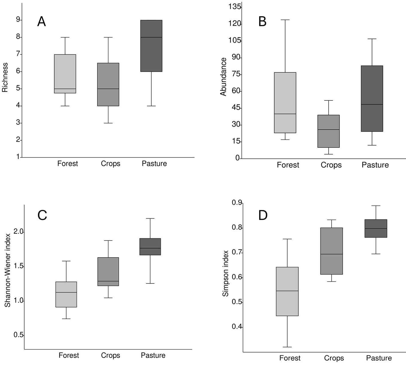
Figure 3. Box plots of richness (A), abundance (B), Shannon Index (C), and Simpson (D) for each of the 3 vegetation covers.

Figure 4. Histogram and box plot of daily ambient temperature across the sampling months; temperature (A, B), rainfall (C).
According to the determined Shannon-Wiener index, the diversity for forest cover was 1,631, crops 1,677, and pasture 2,107. On the other hand, Simpson’s index estimated a dominance of 0.726 for the forest, crops 0.746, and pasture 0.858. When comparing the metrics recorded in each vegetation cover (Fig. 3), the pastures registered on average the greatest richness, abundance, and diversity. The average richness was similar between the crops and the forest; however, the variation was greater in the crops. In contrast, the average and variation of abundance was greater in the forest than in the crops. The average species diversity was lowest in forests, intermediate in crops, and highest in pastures. There were statically differences of all metrics among vegetation cover; richness (one-way ANOVA, F = 5.456, df = 2, p > 0.05), abundance (H(χ2) = 4.63, p > 0.05), Shannon (one-way ANOVA, F = 16.71, df = 2, p > 0.05), and Simpson (H(χ2) = 15.97, p > 0.05).
When we graph the monthly fluctuations of ambient temperature and precipitation (Fig. 4), it is evident that during the days and months of sampling, precipitation was little or none (monthly average from 1.3 mm in January to 7.4 mm in April) whereas monthly average temperature tended to increase from 21.5 °C to 23.3 °C from January to March and from 24.0 to 24.5 °C from April to June. These daily temperature records showed significant monthly differences (ANOVA, F = 67.1, df5 = 5, df2 = 79.8, p < 0.001). There were no significant monthly fluctuations with respect to precipitation (ANOVA, F = 1.78, df5 = 5, df2 = 78.8, p > 0.05). The species richness tended to be higher in April and June in all 3 vegetation covers (Fig. 5) whereas abundance was higher in the forest in March and higher for pastures and crops during April and June. Species diversity (Shannon and Simpson) in the forest was higher in March whereas in both crops and pastures it was higher in June (Fig. 5).
Based on the Jaccard similarity index, crop and pastures presented a greater degree of similarity (Fig. 6), that is, a greater number of shared species. The forest presented the greatest dissimilarity in species composition with respect to the crop and the pasture, having a greater number of unique species (D. truncatus, D. ebraccatus, L. poecilochilus, and L. savagei), which are shown in Table 1.
It was observed that the microhabitat most used by anurans in the forest was leaf litter. The species most associated with this type of microhabitat were D. truncatus and L. poecilochilus (Fig. 7); these species were only recorded in this coverage (Table 1). In the pasture, the highest record of species was found in bare soils and jagüeyes, with L. fuscus, L. insularum, and B. pugnax being the most associated with the latter, while R. horribilis and R. humboldti were observed mainly in bare soil (Fig. 8). In addition, these species presented the highest number of records of individuals in this coverage (Table 1). Finally, in the crop coverage, the microhabitat with the highest number of anuran records was bare soil (Fig. 9), this microhabitat was used most frequently by R. humboldti, R. horribilis, and P. brachyops which were the species with the highest number of individuals recorded; this microhabitat was also used by E. panamensis, which was the only species present in this cover (Table 1).
Discussion
In this study, 19 species of anurans and 1 casual record were identified, for a total of 20 species, this being a slightly smaller number than the 21 species recorded in the SFF Los Colorados 2018-2023 Management Plan (Jiménez et al., 2018). Craugastor raniformis (Boulenger, 1896), Pseudopaludicola pusilla (Ruthven, 1916), and Lectodactylus fragilis (Brocchi, 1877) were not observed in our study, possibly due to lack of sampling in some areas of the SFF Los Colorados. Their occurrence cannot be ruled out, since they were recorded by Acosta-Galvis (2012) in the Montes de María. This study reports C. raniformis in the forest, in ravines (on rocks), on leaf litter, and in shrubby vegetation; P. pusilla in crop areas and on the edge of plain forests, on sandy substrates and in cracks after rains; L. fragilis in flat areas, around seasonal ponds, and near swamps.
Scarthyla, D. ebraccatus, and L. savagei are added to the anuran fauna of the SFF Los Colorados, which shows that it is necessary to continue carrying out studies in the subregions of STDF, including the protected areas of the plains of the Caribbean region, valleys of the Magdalena and Cauca Rivers, Catatumbo, and enclaves of the Patía Valley. Amphibian diversity is poorly known due to the lack of biological studies (Urbina-Cardona et al., 2014).
Sampling carried out in the first 3 months of the year (January, February, and March) regularly corresponds to the dry season (Rangel & Carvajal-Cogollo, 2012). However, rains occurring in these months is a consequence of the effects of the La Niña phenomenon in Colombia for 2022 (Guzmán-Ferraro & García, 2022).
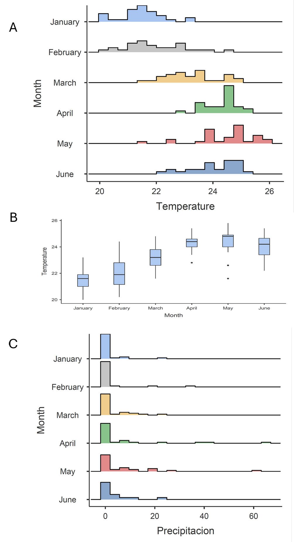
Figure 4. Histogram and box plot of daily ambient temperature across the sampling months; temperature (A, B), rainfall (C).
Increases were observed in the specific richness and in the recorded number of individuals as rainfall increased (especially in April and June), so it was considered that the rainfall regime prior to sampling played an important role in the observation of anurans. These increases in richness and mainly in the number of individuals are attributed to higher activity and the reproductive strategies of some species, which take advantage of the rains to reproduce and lay eggs in temporary ponds. The rains caused greater activity and detectability of some species that were observed vocalizing in small ponds that had formed and cow dams.

Figure 5. Monthly trend of average richness (A), abundance (B), and diversity (C, D) for each vegetation cover type.
Only some amplexuses were recorded but we did not record nesting or reproduction events. Some of the species have explosive activity, which generates an increase in the number of individuals, as is the case of R. horribilis and other species (Vargas-Salinas et al., 2019); some other species vocalizing included Engytomops pustulosus in some ponds and Dendropsophus microcephalus in the emerging vegetation around the cow dams. However, it is worth mentioning that the frequency and intensity of the La Niña phenomenon due to climate change could alter the reproductive times of anurans, causing many species to have early reproduction, which would bring about temporal overlaps of the species that would generate changes in the structure of the assembly (Lawyer & Morin, 1993).
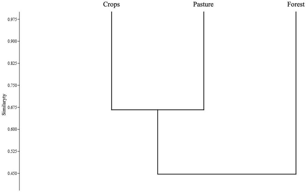
Figure 6. Jaccard similarity dendrogram for the anuran samples from the SFF Los Colorados.
As we expect, there were differences of species richness among vegetation covers. The forest recorded greater richness of anurans than the productive systems (pasture and crops). This is mainly attributed to the greater availability of humid microhabitats and the vegetaion complexity, since there are species that require dense vegetation cover and abundant leaf litter. For example, the oviposition of D. truncatus occurs in humid leaf litter (Cárdenas-Ortega et al., 2019), so different studies record it abundantly in forested areas (Burbano-Yandi et al., 2016; De la Ossa et al., 2016, 2011; Posso-Peláez et al., 2017). On the other hand, pasture and crop are covers with less complexity in the vegetal structure, generating changes in the composition of the anuran assemblages (Cortés-Gómez et al., 2013), such as the reduction in richness, which is closely linked to the reproductive modes of each species (Almeida-Gomes & Rocha, 2015). These same changes in richness in covers with different degrees of disturbance have been recorded in different studies carried out in the Middle Magdalena Valley, in Meta, and in Florencia (Burbano-Yandi et al., 2016; Cáceres-Andrade & Urbina-Cardona, 2009; Duarte-Marín et al., 2018). However, total and monthly average species richness and diversity tended to be higher in the pastures and the lowest in the forests, which registered the greatest monthly variation, recorded the higher species richness and diversity in April and June. The greater diversity of species recorded in pastures may be associated with the lower complexity of the vegetation structure of this habitat, which allows anurans to be easier to detect, while the greater structural complexity of forests and crops decreases detectability of the anurans. Additionally, the presence of jagüeyes in pastures, as sites with availability of water and constant humidity necessary for the survival of the anurans, contributed to the greatest number of records of individuals in this vegetation coverage. Leptodactylus fuscus, L. insularum, and B. pugnax had greater abundance in cow dams of the pasture, since they make postures close to bodies of water (Carvajal-Cogollo et al., 2019; Ortega-Chinquilla et al., 2019).

Figure 7. Use of microhabitats by species in the forest cover of the SFF Los Colorados.
Jagüeyes are considered important for many species in disturbed areas because they permanently provide water resources, which can be used to increase water uptake and reduce evaporation rates (Urbina-Cardona et al., 2014), in addition to be used by species with reproductive modes associated with this resource (Cardozo & Caraballo, 2017). On the other hand, bare soils were mostly used by R. horribilis and R. humboldti, which are species that are commonly found in disturbed areas (Acosta-Galvis, 2012), these have physical characteristics (tuberculated skin) and physiological characteristics that allow them to adapt to exploit this microhabitat (Cáceres-Andrade & Urbina-Cardona, 2009), for this reason, they were found with greater abundance in pastures and crops.
Dendrobates truncatus, D. ebraccatus, L. poecilochilus, and L. savagei are species that were recorded only in the forest, similar to what has been reported by other anuran assemblage studies, where they are not only recorded in forested areas, but also in wetlands (Acosta-Galvis et al., 2006; Angarita et al., 2015; Burbano-Yandi et al., 2016). On the other hand, S. vigilans was only recorded in pastures; in this study the species was observed mainly around bodies of water, specifically on emergent vegetation, in sympatry with D. microcephalus (Muñoz-Guerrero et al., 2007; Fonseca- Pérez et al., 2017). Finally, E. panamensis was only present in crops, although in the study carried out by Blanco-Torres et al. (2015), it was also recorded in pastures. This is a species identified as a leaf miner (Cuentas et al., 2002), which has possibly been the reason why it was observed near the cracks produced by cassava plantations. It is due to all the above that the species similarity analysis showed that the forest differs with respect to the other 2 covers, which are noticeably more similar to each other. Just as we expected, the forest differs in species composition.
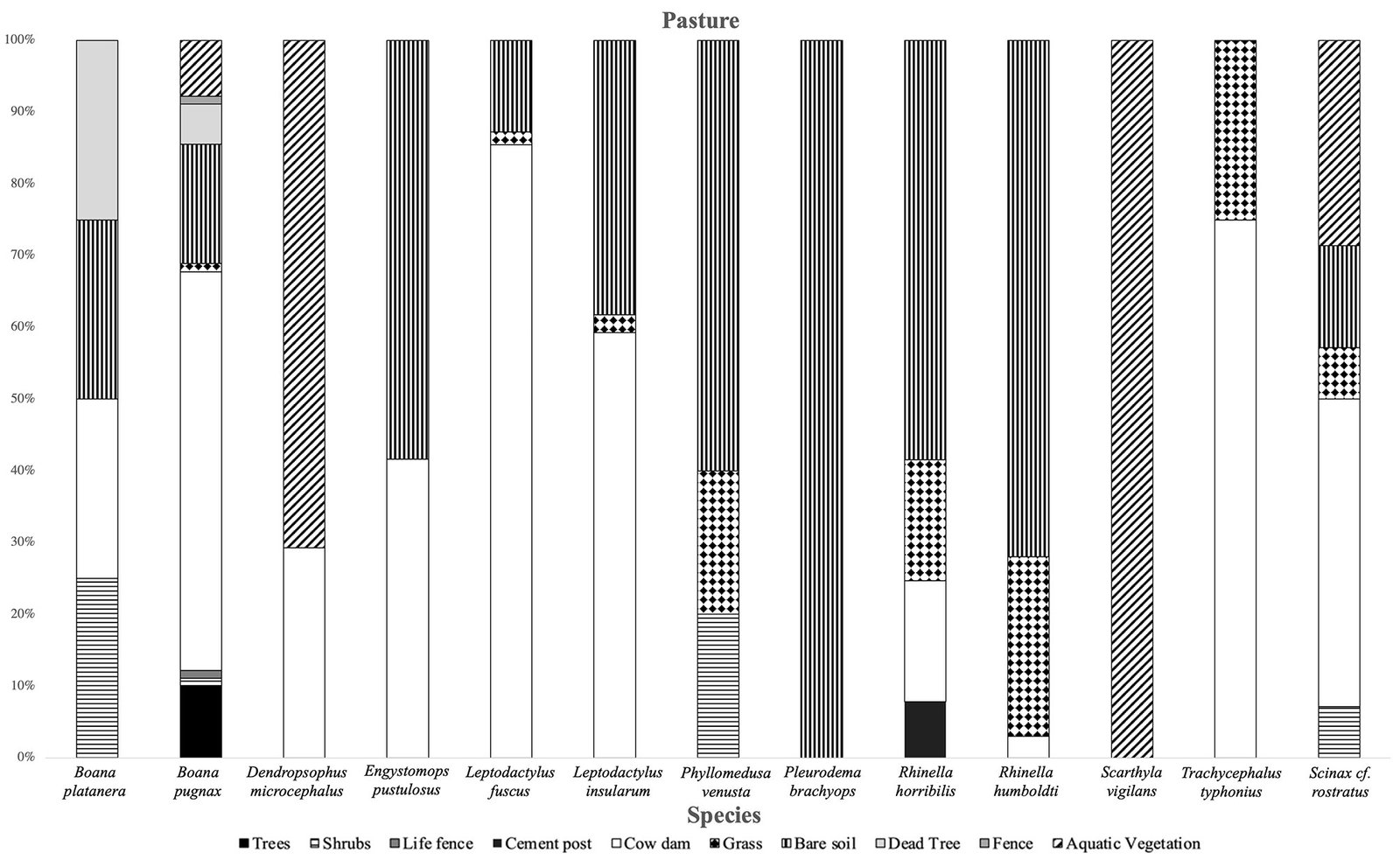
Figure 8. Use of microhabitats by species in the pasture cover of the SFF Los Colorados.
The species diversity index values reported in our study are similar to those obtained in a nearby area located in Meta, Colombia (Cáceres-Andrade and Urbina-Cardona, 2009) where they reported values of 1.4 for humid forest, 1.43 in pastures and 1.9 in sugarcane crops. On the other hand, Román-Palacios et al. (2016) estimated a low Shannon-Wiener index in the Magdalena Medio for forest and quarry (0.92 and 1.74, respectively), while for the lake, they estimated an intermediate diversity (2.03). The forest value was very far from that estimated in this work, which may indicate that the SFF Los Colorados forest has an important conservation status that benefits the anurafauna.
On the other hand, Simpson’s index estimated high dominance for the 3 plant covers. This dominance may be associated with the microhabitats they offer; for example, the forest offered important microhabitats (numerous ponds and abundant leaf litter) for the development of E. pustulosus and D. truncatus, which made these species dominant in this cover. On the other hand, the crop was dominated mainly by P. brachyops, R. humbolbti, and R. horribilis; these species have terrestrial habits, tolerant to landscape transformations and abundant open environments (Acosta-Galvis, 2012; Rodríguez-Molina, 2004). Finally, the pasture was dominated by species of the genus Rhinella and Leptodactylus, where the latter has reproductive modes associated with foam nests, allowing them to conquer and be abundant in anthropized environments (Alcaide et al., 2012).
Jaccard’s similarity analysis for the anurans of the SFF Los Colorados indicates a grouping between pasture and crop cover due to the percentage of shared species (66.6%). This result may be associated with the fact that both covers are intervened areas, with a vegetation structure different from that of the forest and host generalist species (e.g., P. brachyops, B. pugnax, L. fuscus) that can share in greater quantities, while the forest, due to the resources it offers, may have species that do not tolerate landscape transformations (e.g., D. truncatus), being restricted only to forested areas (Cáceres-Andrade & Urbina-Cardona, 2009).

Figure 9. Use of microhabitats by species in the crop cover of the SFF Los Colorados.
The results of this research indicate that the transformation of the landscape because of the agricultural economy of the Montes de María, based mainly on cultivation and the raising of animals (Aguilera-Díaz, 2013), generated changes in the wealth, abundance, composition and use of microhabitats in anuran assemblages. Therefore, this knowledge is important to create concrete tools for the management and conservation of these organisms in the protected area and its surroundings, such as maintaining native vegetation and layers of leaf litter in productive systems, conserving lentic and lotic water sources, and reducing the use of agrochemicals, among others (Urbina-Cardona et al., 2015).
This research constitutes the baseline to evaluate the long-term response of anurans to ecological restoration processes and initiatives led by the SFF Los Colorados team in transformed areas of the protected area. This research constitutes the baseline to evaluate the long-term response of anurans to ecological restoration processes and initiatives led by the SFF Los Colorados team in transformed areas of the protected area. Results that could be useful in future studies where reference ecosystems (conserved areas) and disturbed areas in the process of restoration are used, to determine if these protected areas are achieving the expected objectives and if they are contributing to the conservation of anurans (Urbina-Cardona et al., 2015). Additionally, this study updates the list of anuran species in the protected area, pointing out those to a specific coverage and those shared among covers (forest, pasture, and crops), which can be useful to define those that may be vulnerable to fragmentation of the habitat or to be included as conservation target values (VOC) of the SFF Los Colorados in the construction of future Management Plans.
Acknowledgments
We thank the Hydrobiology research group of the University of Cartagena for providing their equipment for the development of this research. Likewise, to the University of Cartagena, for the financial support through resolution number 01878 of 2022. To IDEAM for providing information on the environmental variables for 2022. To Gabriel R. Navas-S, Dr. Andrés García, and Vivarium del Caribe for financial support and suggestions for carrying out this study. Likewise, to the technical and administrative team of the Los Colorados Flora and Fauna Sanctuary for their support in sampling, logistics, loan of facilities, and management of the research guarantee. To Joselin Castro-Palacios for his support in the implementation of the methodology of this work and to Adolfo A. Mulet-Paso for his suggestions in the identification of the species. To David Gernandt, for his revision to the text which improved substantially.
References
Acosta-Galvis, A. R. (2012). Anfibios de los enclaves secos del área de influencia de los montes de María y la ciénaga de La Caimanera, departamento de Sucre, Colombia. Biota Colombiana, 13, 211–255.
Acosta-Galvis, A. R. (2021). Lista de anfibios de Colombia. BATRACHIA. Retrieved on June 17, 2021 from: http://www.batrachia.com
Acosta-Galvis, A. R., Huertas-Salgado, C., & Rada, M. (2006). Aproximación al conocimiento de los anfibios en una localidad del Magdalena medio (Departamento de Caldas, Colombia). Revista de la Academia Colombiana de Ciencias Exactas, Físicas y Naturales, 30, 291–303. https://doi.org/10.18257/raccefyn.30(115).2006.2250
Acuña-Vargas, J. C. (2016). Anfibios y reptiles asociados a cinco coberturas de la tierra, municipio de Dibulla, La Guajira, Colombia. Acta Zoológica Mexicana, 32,133–146. https://doi.org/10.21829/azm.2016.322940
Aguilera-Díaz, M. M. (2013). Montes de María: una subregión de economía campesina y empresarial. Cartagena: CEER.
Aguirre-León, G. (2011). Métodos de estimación, captura y contención de anfibios y reptiles. Manual de Técnicas para el estudio de la Fauna. In S. López-González y C. López-González (Eds.), Manual de técnicas para el estudio de fauna (pp. 61–85). Querétaro: Universidad Autónoma de Querétaro, A.C.
Alcaide, A. P., Ponssa, M. L., Alcaide, F. P., & Alcaide, M. (2012). Histología de ovario en hembras vitelogénicas de Leptodactylus latinasus (Anura, Leptodactylidae). Acta Zoológica Lilloana, 56, 44–53.
Almeida-Gomes, M., & Rocha, C. F. (2015). Habitat loss reduces the diversity of frog reproductive modes in an Atlantic Forest fragmented landscape. Biotropica, 47, 113–118. https://doi.org/10.1111/btp.12168
Andrade, M. G. (2011). Estado del conocimiento de la biodiversidad en Colombia y sus amenazas. Consideraciones para fortalecer la interacción ciencia-política. Revista de la Academia Colombiana de Ciencias Exactas, Físicas y Naturales, 35, 491–508.
Angarita, M. O., Montes-Correa, A. C., & Renjifo, J. M. (2015). Amphibians and reptiles of an agroforestry system in the Colombian Caribbean. Amphibian and Reptile Conservation, 8, 33–52.
Blanco, A., & Bonilla, M. (2010). Partición de microhábitats entre especies de Bufonidae y Leiuperidae (Amphibia: Anura) en áreas con bosque seco tropical de la región Caribe-Colombia. Acta Biológica Colombiana, 15,47–60.
Blanco-Torres, A., Duré, M., & Bonilla, M. A. (2015). Observaciones sobre la dieta de Elachistocleis pearsei y Elachistocleis panamensis en dos áreas intervenidas de tierras bajas del norte de Colombia. Revista Mexicana de Biodiversidad, 86,538–540. https://doi.org/10.1016/j.rmb.2015.04.031
Ballesteros-Correa, J., Vidal-Pastrana, C., & Ortega-León, A. M. (2019). Anfibios de Córdoba, Colombia. Córdoba: Fondo Editorial de Córdoba.
Burbano-Yandi, C. E., Gómez-Díaz, M. A., Gómez-Figueroa, A., Velásquez-Trujillo, D. A., & Bolívar-García, W. (2016). Ensamblaje de anfibios presentes en un bosque seco y en sistemas productivos, Valle Medio del Magdalena, Victoria y La Dorada, Caldas, Colombia. Revista de Ciencias, 20, 81–93.
Cáceres-Andrade, S. P., & Urbina-Cardona, J. N. (2009). Ensamblajes de Anuros de sistemas productivos y bosques en el Piedemonte Llanero, departamento del Meta, Colombia. Caldasia, 31, 175–195.
Cárdenas-Ortega, M. S., Gutiérrez-Cárdenas, P. D., Cifuentes-Ortegón, M., & Patiño-Gallego, A. M. (2019). Dendrobates truncatus (Cope, 1861) Rana venenosa de rayas amarillas. Catálogo de Anfibios y Reptiles de Colombia, 5, 32–41.
Cardozo, J., & Caraballo, P. (2017). Fauna anura (Amphibia: Anura) asociada a jagüeyes en dos localidades de la región Caribe colombiana. Revista Colombiana de Ciencia Animal-RECIA, 9, 39–47. https://doi.org/10.24188/recia.v9.nS.2017.519
Carvajal-Cogollo, J. E., Bernal-González, V., Paternina-Hernández, A., Muñoz-Ávila, J. N., & Vargas-Salinas, F. (2019). Uso de hábitat y reglas de ensamble: patrones y mecanismos. In M. H. Restrepo-Domínguez, E. Vera-López, Y. Bolívar-Suárez, S. G. Numpaque-Piracoca, O. Y. Acuña-Rodríguez, Z. Z. Ojeda-Pérez et al. (Eds.), Biología de los anfibios y reptiles en bosque tropical del norte de Colombia (pp. 297–338). Tunja: Editorial UPTC.
Clarke, K. R., Gorley, N. R., Somerfield, P. J., & Warwick, R. M. (2014). Change in marine communities: an approach to statistical analysis and interpretation. Plymouth: PRIMER-E.
Colwell, R. K., & Coddington, J. A. (1994). Estimating terrestrial biodiversity through extrapolation. Philosophical Transactions of the Royal Society of London. Series B: Biological Sciences, 345,101–118. https://doi.org/10.1098/rstb.1994.0091
Conell, J. H. (1978). Diversity in tropical rain forests and coral reefs. Science, 199,1302–1310. http://dx.doi.org/10.1126/science.199.4335.1302
Cortés-Gómez, A. M., Castro-Herrera, F., & Urbina-Cardona, J. N. (2013). Small changes in vegetation structure create great changes in amphibian ensembles in the Colombian Pacific rainforest. Tropical Conservation Science, 6, 749–769. https://doi.org/10.1177/194008291300600604
Cortez, F. C., Suárez-Mayorga, A. M., & López-López, F. J. (2006). Preparación y preservación de material científico. In A. Angulo, J. V. Rueda-Almonacid, J. V. Rodríguez-Mahecha y E. La Marca (Eds.), Técnicas de inventario y monitoreo para los anfibios de la región tropical andina (pp. 173–218). Bogotá: Panamericana Formas e Impreso S.A.
Cristal, A., Sánchez, E., Romero, J., Leyva, J., Andrade, W., & Buelvas, C. (2020). ¿Qué hemos logrado con el proyecto de Conectividades Socio-Ecosistémicas? La evolución de la metodología de las 4Ps: avances y retos. In A. Cristal, M. Peña y J. Ferrer-Sotelo (Eds.), El proyecto de conectividades Socio-Ecosistémicas en los Montes de María, 2013–2020 (pp. 63–87). Bogotá-Colombia: Fundación Herencia Ambiental Caribe.
Crump, M., & Scott, N. (2001). Relevamiento por encuentros visuales. In W. R. Heyer, M. A. Donnelly, R. W. Diarmid, L. C. Hayek, & M. S. Foster (Eds.), Medición y monitoreo de la diversidad biológica: métodos estandarizados para anfibios (pp. 80–86). Chubut, Argentina: Editorial Universitaria de la Patagonia.
Cuentas, D., Borja, R., Lynch, J. D., & Renjifo, J. M. (2002). Anuros del departamento del Atlántico y norte de Bolívar. Barranquilla: Editorial Cencys.
De Sá, R. O. (2005). Crisis global de biodiversidad: importancia de la diversidad genética y la extinción de anfibios. Agrociencia, 9, 513.
De la Ossa, J., Contreras-Gutiérrez, J. C., & Campillo-Castro, J. (2011). Censo de Dendrobates truncatus (Anura, Dendrobatidae) en la reserva forestal protectora Serranía de Coraza, Montes de María, Sucre, Colombia. Revista Colombiana de Ciencia Animal-RECIA, 3, 339–343. https://doi.org/10.24188/recia.v3.n2.2011.407
Díaz, S., Fargione, J., Chapin, F. S., & Tilman, D. (2006). Biodiversity loss threatens human well-being. Plos Biology, 4, 1300–1305. https://doi.org/10.1371/journal.pbio.0040277
Duarte-Marín, S., González-Acosta, C., & Vargas-Salinas, F. (2018). Estructura y composición de ensamblajes de anfibios en tres tipos de hábitat en el Parque Nacional Natural Selva de Florencia, Cordillera Central de Colombia. Revista de la Academia Colombiana de Ciencias Exactas, Físicas y Naturales, 42, 227–236. https://doi.org/10.18257/raccefyn.631
Dunn, E. R. (1944). Los géneros de anfibios y reptiles de Colombia. Caldasia, 2,497–529.
Echeverry, M. A., & Rodríguez, J. M. (2006). Análisis de un paisaje fragmentado como herramienta para la conservación de la biodiversidad en áreas de bosque seco y subhúmedo tropical en el municipio de Pereira, Risaralda Colombia. Scientia et Technica, 12, 405–410.
Etter, A., Andrade, A., Saavedra, K., Amaya, P., Cortés, J., Pacheco, C. et al. (2017). Lista Roja de Ecosistemas de Colombia, 2,1–6. https://doi.org/10.13140/RG.2.2.10861.08165
Etter, A., McAlpine, C., & Possingham, H. (2008). Historical patterns and drivers of landscape change in Colombia since 1500: a regionalized spatial approach. Annals of the Association of American Geographers, 98, 2–23. https://doi.org/10.1080/00045600701733911
Fonseca-Pérez, K. A., Molina, C., & Tárano, Z. (2017). Diet of Dendropsophus microcephalus and Scarthyla vigilans (Anura: Hylidae) at a locality in north-western Venezuela with notes on microhabitat occupation. Papéis Avulsos de Zoologia, 57,93–104. https://doi.org/10.11606/0031-1049.2017.57.07
Fox, B. J., Taylor, J. E., Fox, M. D., & Williams, C. (1997). Vegetation changes across edges of rainforest remnants. Biological Conservation, 82, 1–13. https://doi.org/10.1016/S0006-3207(97)00011-6
Galván-Guevara, S., Ballut-Dajud, G., & De La Ossa, J. (2015). Determinación de la fragmentación del bosque seco del arroyo Pechelín, Montes de María, Caribe, Colombia. Biota Colombiana, 16, 149–157.
García, R. J. C., Castro, H. F., & Cárdenas, H. H. (2005). Relación entre la distribución de anuros y variables del hábitat en el sector La Romelia del Parque Nacional Natural Munchique (Cauca, Colombia). Caldasia, 27, 299–310.
García, H., Corzo, G., Isaacs, P., & Etter, A. (2014). Distribución y estado actual de los bosques remanentes del bioma de bosque seco tropical en Colombia: insumos para su gestión. In C. Pizano, & H. García (Eds.), El bosque seco tropical en Colombia (pp. 228–251). Bogotá: Instituto de Investigación de Recursos Biológicos Alexander von Humboldt.
Guzmán-Ferraro, M., & García, G. (2022). El fenómeno de La Niña persistirá hasta casi la mitad del año. CVC. Retrieved on January 14th, 2022 from: http://www.cvc.gov.co/boletin-prensa-007-2022
Hammer, Ø., Harper, D. A., & Ryan, P. D. (2001). PAST: Paleontological statistics software package for education and data analysis. Palaeontologia Electronica, 4, 1–9.
Herazo, F., Mercado, J., & Mendoza, H. (2017). Estructura y composición florística del bosque seco tropical en los Montes de María (Sucre-Colombia). Ciencia en Desarrollo, 8,71–8.
Instituto Alexander von Humboldt. (1998). El bosque seco tropical en Colombia B-sT. Grupo de Exploraciones y Monitoreo Ambiental. Bogotá, Colombia.
IDEAM (Instituto de Hidrología, Meteorología y Estudios Ambientales), IGAC (Instituto Geográfico Agustín Codazzi), & CORMAGDALENA (Corporación Autónoma Regional del río Grande de La Magdalena). (2008). Mapa de cobertura de la Tierra Cuenca Magdalena-Cauca: Metodología CORINE Land Cover adaptada para Colombia a escala 1:100.000. Bogotá: IDEAM/ IGAC/ CORMAGDALENA.
Jiménez, B., De la Rosa, N., & Naranjo, D. (2018). Plan de manejo del Santuario de Flora y Fauna Los Colorados. Parques Nacionales Naturales de Colombia. Santa Marta: Dirección Territorial Caribe.
Laurance, W. F., & Gascon, C. (1997). How to creatively fragment a landscape. Conservation Biology, 11, 577–579.
Lawler, S., & Morin, P. (1993). Temporal overlap, competition, and priority effects in larval anurans. Ecology, 71, 174–182. https://doi.org/10.2307/1939512
Magurran, A. (2004). Measuring biological diversity. Malden: Blackwell Publishing.
Manzanilla, J., & Péfaur, J. E. (2000). Consideraciones sobre métodos y técnicas de campo para el estudio de anfibios y reptiles. Revista de Ecología Latinoamericana, 7,17–30.
Marín, A. M., Ríos, L., Ríos, L., & Almario, J. (2017). Impacto de la actividad ganadera sobre el suelo en Colombia. Ingeniería y Región, 17, 1–12. https://doi.org/10.25054/issn.2216-1325
Meza-Tílvez, K., Mulet-Paso, A., & Zambrano-Cantillo, R. (2018). Fauna del Jardín Botánico de “Guillermo Piñeres” de Cartagena, Turbaco, Colombia: Anfibios y reptiles. Versión 1. Chicago, Illinois: Field Museum.
Moreno, C. E. (2001). Métodos para medir la biodiversidad. Volumen 1. Zaragoza: CYTED, ORCYT/ UNESCO & SEA.
Muñoz-Guerrero, J., Serrano, V. H., & Ramírez-Pinilla, M. P. (2007). Uso de microhábitat, dieta y tiempo de actividad en cuatro especies simpátricas de ranas hílidas neotropicales (Anura: Hylidae). Caldasia, 29, 413–425.
McDiarmid, R. W. (1994). Preparing amphibians as scientific specimens. In W. R. Heyer, M. A. Donnelly, R. W. McDiarmid, L. C. Hayek, & M. S. Foster (Eds.), Measuring and monitoring biological diversity. standard methods for amphibians (pp: 289–296). Washington D.C.: Smithsonian Institution Press.
O’Malley, B. (2007). Anatomía y fisiología clínica de animales exóticos. Zaragoza: Servet.
Ortega-Chinquilla, J., Méndez-Narváez, J., Carvajalino-Fernández, J., & Galindo-Uribe, D. (2019). Ecofisiología. In F. Vargas-Salinas, J.A. Muñoz-Avila & M.E. Morales-Puente (Eds.), Biología de los anfibios y reptiles en bosque tropical del norte de Colombia (pp. 297–338). Tunja: Editorial UPTC.
Pizano, C., Gonzáles, R., Gonzáles, M., Castro-Lima, R., Rodríguez, N., Idárraga, A. et al. (2014). Plantas de los bosques secos de Colombia. In C. Pizano, & H. García (Eds.), El bosque seco tropical en Colombia (pp. 228–251). Bogotá: Instituto de Investigación de Recursos Biológicos Alexander von Humboldt.
Posso-Peláez, C., Blanco-Torres, A., & Gutiérrez-Moreno, L. C. (2017). Uso de microhábitats, actividad diaria y dieta de Dendrobates truncatus (Cope, 1861) (Anura: Dendrobatidae) en bosque seco tropical del norte de Colombia. Acta Zoológica Mexicana, 33, 490–502.
Rangel, C. J. O., & Carvajal-Cogollo, J. E. (2012). Clima de la región Caribe Colombiana. In J. O. Rangel (Ed.), Colombia diversidad biótica XII: la región Caribe de Colombia (pp. 67–129). Bogotá: Instituto de Ciencias Naturales.
Re:wild, Synchronicity Earth, IUCN SSC Amphibian Specialist Group. (2023). State of the World’s Amphibians: The Second Global Amphibian Assessment. Texas: Re:wild. Electronic source at the IUCN website
Rodríguez-Molina, C. R. (2004). Reproducción de Pleurodema brachyops (Anura: Lectodactylidae) en los llanos del Estado Apure, Venezuela. Memoria de la Fundación La Salle Ciencias Naturales, 2002, 117–125.
Rodríguez, G. M., Banda, K., Reyes, S. P., & Estupiñán-González, A. C. (2012). Lista comentada de las plantas vasculares de bosques secos prioritarios para la conservación en los departamentos de Atlántico y Bolívar (Caribe colombiano). Biota Colombiana, 13, 7–39.
Rojas, R. R., & Pérez-Peña, P. E. (2018). Evidencia preliminar del efecto borde en anfibios de la Reserva Nacional Pucacuro, al norte de la Amazonía peruana. Revista del Instituto de Investigaciones de la Amazonía Peruana, 27, 55–67.
Romero, H. G. (2013). Deforestación en Colombia: retos y perspectivas. In F. Dane (Ed.), El desafío del desarrollo sustentable en América Latina (pp. 123–142). Río de Janeiro: SOPLA.
Román-Palacios, C., Fernández-Garzón, S., Hernández, M., Ishida-Castañeda, J., Gallo-Franco, W., & Bolívar-García, A. (2016). Uso de microhábitat por anuros en un fragmento de bosque seco intervenido del Magdalena Medio, Guarinocito, Caldas. Boletín Científico Centro de Museos Museo de Historia Natural, 20, 181–196. https://doi.org/10.17151/bccm.2016.20.2.14
Salvador, J., & Gómez, D. (2018). Reptiles y anfibios del departamento del Atlántico, Colombia. Versión 3. Bogotá, Colombia: Field Museum-Museo de Historia Natural ANDES.
Stuart, S. N., Chanson, J., Cox, N.A., & Young, B. E. (2006). Estado global de los anfibios. In A. Angulo, J. V. Rueda-Almonacid, J. V. Rodríguez-Mahecha, & E. La Marca (Eds.), Técnicas de inventario y monitoreo para los anfibios de la región tropical andina (pp. 19–41). Bogotá: Panamericana Formas e Impreso S.A.
Simmons, J. E., & Muñoz-Saba, Y. (Eds.). (2005). Cuidado, manejo y conservación de las colecciones biológicas. Bogotá: Universidad Nacional de Colombia.
Thompson, P. L., Rayfield, B., & González, A. (2017). Loss of habitat and connectivity erodes species diversity, ecosystem functioning, and stability in metacommunity networks. Ecography, 40, 98–108. https://doi.org/10.1111/ecog.02558
Urbina-Cardona, J. N., Olivares-Pérez, M., & Reynoso, V. H. (2006). Herpetofauna diversity and microenvironment correlates across a pasture-edge-interior ecotone in tropical rainforest fragments in the Los Tuxtlas Biosphere Reserve of Veracruz, Mexico. Biological Conservation, 132,61–75. https://doi.org/10.1016/j.biocon.2006.03.014
Urbina-Cardona, J. N., Arturo-Navas, C., Gonzales, I., Gómez-Martínez., M. J., Llano-Mejía, J., Medina-Rangel, G. F. et al. (2014). Determinantes de la distribución de los anfibios en el bosque seco tropical de Colombia: herramientas para su conservación. In H. Pizano, & H. García (Eds.), El bosque seco tropical en Colombia (pp. 169–195). Bogotá: Instituto de Investigación de Recursos Biológicos Alexander von Humboldt.
Urbina-Cardona, J. N., Bernal, E. A., Giraldo-Echeverry, N., & Echeverry-Alcendra, A. (2015). El monitoreo de herpetofauna en los procesos de restauración ecológica: indicadores y métodos. Monitoreo a procesos de restauración ecológica, aplicado a ecosistemas terrestres. Bogotá: Instituto de Investigación de Recursos Biológicos Alexander von Humbold.
Vargas-Salinas, F., Angarita-Sierra, T., Ospinal, L. A., Rocha-Úsuga, A., & Rueda-Solano, L. (2019). Comunicación y ecología reproductiva. In F. Vargas-Salinas, J.A. Muñoz-Avila & M.E. Morales-Puente (Eds.), Biología de los anfibios y reptiles en bosque tropical del norte de Colombia (pp. 297–338). Tunja: Editorial UPTC.
Vargas, S. F., & Bolaños, L. M. E. (1999). Anfibios y reptiles presentes en hábitats perturbados de selva lluviosa tropical en el bajo Anchicayá, Pacífico colombiano. Revista de la Academia Colombiana de Ciencias Exactas, Físicas y Naturales, 23,499–511.
Villareal, H. M., Álvarez, M., Córdoba-Córdoba, S., Escobar, F., Fagua, G., Gast, F. et al. (2004). Manual de métodos para el desarrollo de inventarios de biodiversidad. Bogotá: Instituto de Investigación de Recursos Biológicos Alexander von Humboldt.
Zug, G. R., Vitt, L., & Caldwell, J. P. (2001). Herpetology: an introductory biology of amphibians and reptiles. San Diego: Academic Press.

Association of Myianoetus sp. (Acari: Histiostomatidae) with necrophagous fly Compsomyiops fulvicrura (Diptera: Calliphoridae), in the Prepuna ecoregion (Jujuy: Argentina)
María Laura Fernández-Salinas a, *, Marcia Luciana Matoz-Fernández b
a Universidad Nacional de Jujuy, Instituto de Biología de la Altura, Avenida Bolivia 1661, 4600 San Salvador de Jujuy, Jujuy, Argentina
b Universidad Nacional de Mar del Plata, Laboratorio de Zoonosis Parasitarias, Funes 3350, 7600 Mar del Plata, Buenos Aires, Argentina
*Corresponding author: mfernandez@inbial.unju.edu.ar (M.L. Fernández-Salinas)
Received: 31 January 2024; accepted: 10 June 2024
Abstract
The genus Myianoetus Oudemans(Acari: Histiostomatidae) is commonly associated with carrion, utilizing flies (Diptera) from various families as a means of dispersal through phoresy. The objective of this paper is to present a new association between Myianoetus sp. mites and Calliphoridae flies and discuss its relevance in forensic sciences. Samples were collected in 3 locations in the Prepuna ecoregion of Jujuy, Argentina. Specimens were captured using necrotraps baited with cow lung. Flies carrying phoretic mites were separated and identified to a specific level, while mites were counted and identified at the lowest possible taxonomic level. Compsomyiops fulvicrura (Robineau-Desvoidy) (Diptera: Calliphoridae) was the only species that presented attached mites, with an average intensity of 12.26 mites per fly. The mites carried by C. fulvicrura were identified as deutonymphs of Myianoetus sp., with a prevalence of 2.56% of infested flies. Significant differences in the abundance of flies with mites were observed between locations and seasons. This article represents the first contribution to knowledge on the specific association between Myianoetus sp. and C. fulvicrura. These findings in forensic ecology are relevant for their potential contribution and application in the development of more precise methods in specific forensic cases.
Keywords: Astigmata; Diptera; Forensic Acarology; Phoresy; New report
© 2024 Universidad Nacional Autónoma de México, Instituto de Biología. Este es un artículo Open Access bajo la licencia CC BY-NC-ND
(http://creativecommons.org/licenses/by-nc-nd/4.0/).
Asociación de Myianoetus sp. (Acari: Histiostomatidae) con la mosca necrófaga Compsomyiops fulvicrura (Diptera: Calliphoridae), en la ecoregión Prepuna (Jujuy: Argentina)
Resumen
El género Myianoetus Oudemans (Acari: Histiostomatidae) suele asociarse a la carroña utilizando moscas (Diptera) de distintas familias como medio de dispersión, a través de la foresia. El objetivo de este trabajo fue presentar una nueva asociación entre Myianoetus sp. con moscas Calliphoridae y discutir su alcance dentro de las ciencias forenses. Las muestras se recolectaron en 3 localidades de la Prepuna jujeña, Jujuy, Argentina. Los especímenes se capturaron mediante necrotrampas cebadas con pulmón vacuno. Las moscas con ácaros se separaron y determinaron a nivel específico; los ácaros fueron numerados e identificados al nivel taxonómico más bajo posible. Compsomyiops fulvicrura (Diptera: Calliphoridae) fue la única especie que presentó ácaros adheridos, con una intensidad media de 12.26 ácaros por mosca. Los ácaros fueron identificados como deutoninfas de Myianoetus sp. y se determinó una prevalencia de 2.56% de moscas infestadas. Se observaron diferencias significativas en la abundancia de moscas con ácaros entre las localidades y estaciones analizadas. Este artículo representa el primer aporte al conocimiento sobre la asociación específica entre Myianoetus sp. y C. fulvicrura. Estos hallazgos sobre ecología forense son relevantes por su potencial contribución y aplicación al desarrollo de métodos más precisos en casos forenses determinados.
Palabras clave:Astigmata; Diptera; Acarología forense; Foresia; Nuevo reporte
Introduction
Carcasses present limited and ephemeral biocenosis made up of diverse organisms that often comprise complex food webs (Braig & Perotti, 2009; Perotti et al., 2010). Many Diptera species actively participate in the cadaveric decomposition process in which the Calliphoridae and Sarcophagidae families, along with Coleoptera are often investigated because of their large number, persistence and capacity to act as hosts to diverse mites that use them for dispersion by phoresis (Camerick, 2010; Perotti & Braig, 2009; Perotti et al., 2010).
Mites present morphological and physiological adaptations to serve phoresy during adult and nymphal stages. These adaptations are documented in the order Mesostigmata, in the suborder Prostigmata and in the infraorder Astigmatina (Oribatida) (Perotti et al., 2010). Astigmata mites are specialists in irregular or ephemeral habitats which they colonize through a deutonymphal heteromorphic stage known as hypopus which is specialized for phoresy (OConnor, 2009). Astigmatid deutonymphs are morphologically simplified, have lost the mouth and chelicerae, have greatly reduced the remainder of the gnathosoma, and have suckers on the paraproctal region for efficient phoretic attachment. The body is strongly dorsoventrally flattened, heavily sclerotized and much more resistant to desiccation than other stages of the life cycle (Farish & Axtell, 1971; OConnor, 1982). The conditions needed to reach this stage may involve genetic factors and physicochemical factors from the environment (Greenberg & Carpenter, 1960).
Astigmatid mites are particularly important for the 3 areas of forensic entomology: urban, stored product pests and medico-legal (Catts & Goff, 1992; Perotti & Braig, 2019). Nevertheless, they often go unnoticed because of their small size. Moreover, their analysis is limited because of difficulties in species identification, lack of specific knowledge and misuse of forensic methodology (OConnor, 2009; Perotti et al., 2010). Numerous species of mites are compulsory or facultative inhabitants of carrion. They are found not only in legal cases that involve human carcasses (Pimsler et al., 2016; Rai et al., 2020; Russell et al., 2004; Saloña-Bordas & Perotti, 2015); but also, in experimental studies concerning faunal succession in animal remains (Arnaldos et al., 2005; Barton et al., 2014; Centeno & Perotti, 1999; Heo et al., 2021).
In Argentina, the only record of the presence of phoretic mites associated with decomposing remains were the preliminary observations of Centeno and Perotti (1999), in which they found mites of the genus Myianoetus Oudemans (Astigmata: Histiostomatidae) associated with a specimen of Morellia sp. (Muscidae). In order to contribute to the further study on phoretic relations between mites and arthropods, this paper presents a new association between mites and Diptera from the Calliphoridae family in Prepuna of Jujuy, Argentina, and discusses its relevance and importance within the forensic sciences.
Materials and methods
The collection of Diptera specimens was carried out in the following locations: Tres Cruces (22°55’06.01” S, 65°35’13.58” W), Humahuaca (23°12’14.27” S, 65°20’54.90” W), and Tumbaya (23°51’27.79” S, 68°28’03.31” W) (Fig. 1a-c). These locations are part of the Monte Province, Prepuna District in the province of Jujuy, Argentina. Two sampling campaigns were carried out, one during the dry season (June, July, and August) and the other during the wet season (December, January, and February) between 2016 and 2018. Each location was equipped with 18 traps, totaling 54 traps across all sampling locations, totaling 108 traps per year.
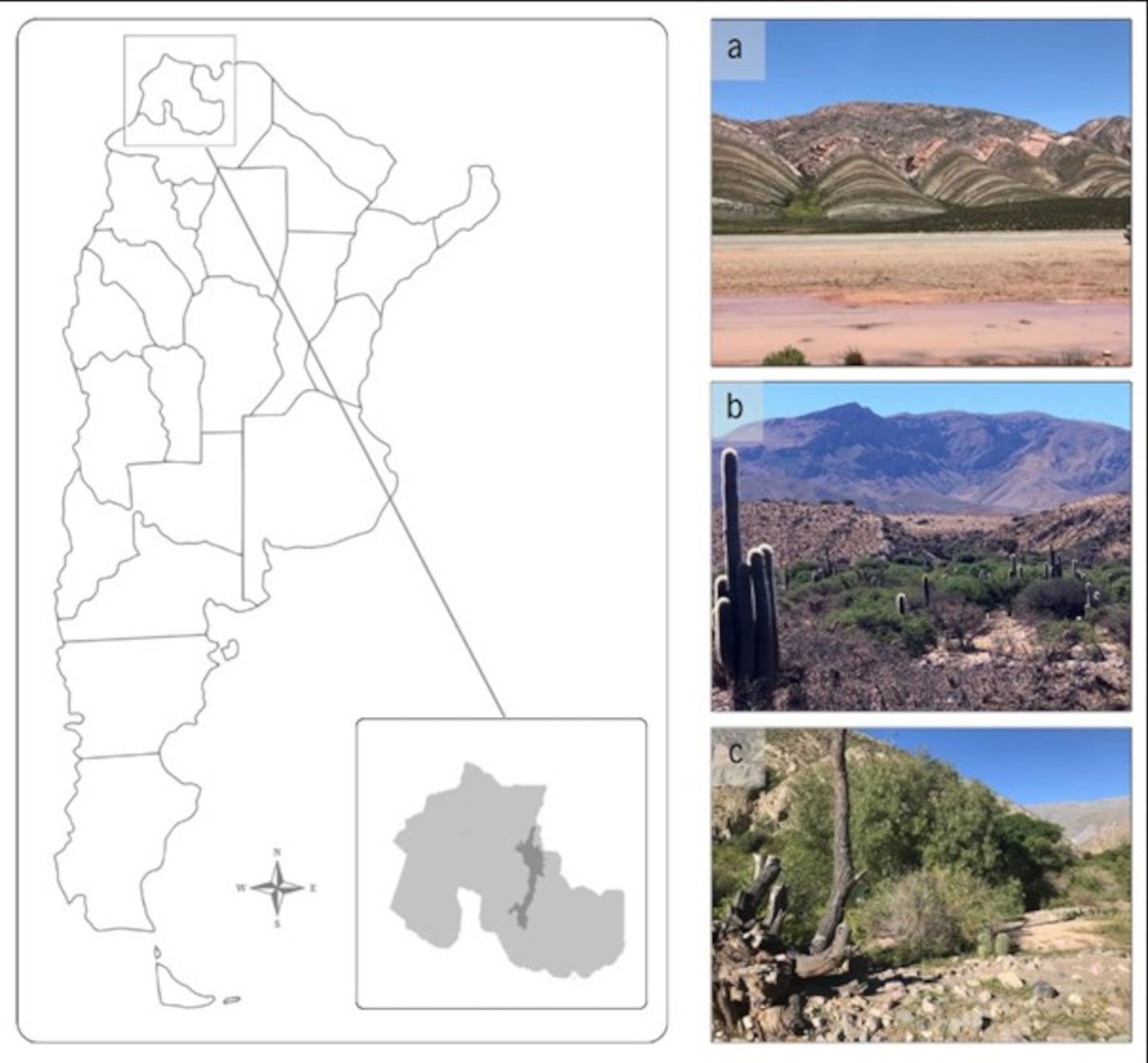
Figure 1. Location of the study area. The map depicts the region corresponding to the Monte Province, Prepuna District, in the province of Jujuy, Argentina. Study sites are located in the following localities: a) Tres Cruces, b) Humahuaca, and c) Tumbaya (Photos by Fernández Salinas, M. L.).
To obtain specimens in good condition for identification, traps were made following Hwang and Turner (2005) (Fig. 2). A modified cone trap, based on a soft drink bottle with a baited target, was constructed. The bottle traps were assembled using two 3 L clear plastic soft drink bottles with a diameter of 11.5 cm, along with a black acrylic container 11 cm measured in diameter and 13 cm in depth. Consisted of 2 parts, the upper collection chamber and the lower bait chamber. The collection chamber was formed from the bottles cut 24 cm and 12 cm from the top respectively, one pushed inside the other (so that the bottle’s spout acts as a funnel and prevents flies from escaping). The bait chamber was made with a black container so the flies were drawn upwards, into the transparent collection chamber. The 2 halves of the trap were push-fitted together and secured by strips of waterproof adhesive tape. To facilitate the entry of flies 4 holes of approximately 0.8 cm in diameter were made around the bait chamber. A 125 cm³ plastic container with the bait was placed at the base of this container. A feeding substrate made of 100 g of cow’s lung was used. A distance of approximately 100 m was maintained between the traps because of the competitive nature of the colonizing species and were separated from the floor as they were hung at a minimum height of 1.5 m to avoid the attack of scavenger mammals. It was placed in a closed recipient which was subjected to a warm temperature between 15 °C and 30 °C, during 60 hours, for sufficient time to decompose. The traps were left in place for 7 consecutive days.
The captured specimens were put in Kahn tubes with 70% alcohol and they were transported to the Institute of Altitude Biology (INBIAL), San Salvador de Jujuy, Jujuy, Argentina.

Figure 2. Design of the bottle necrotrap baited with cow lung.
Flies that presented mites were counted, separated by sex and identified to its most specific level using keys and revisions from Olea and Mariluis (2013), Whitworth (2014), and Mulieri et al. (2014). The flies were photographed “in situ” using a Canon 5D Mark IV camera, 3 extension tubes for macro photography and a Canon 85 mm 1.8 lens illuminated with a Godox AD200 flash and a Godox V860 flash. Afterward, the specimens were sent to the Parasitic Zoonoses Laboratory, National University of Mar del Plata, Mar del Plata, Buenos Aires, Argentina. Each fly was individually examined, and the number of mites per fly and their attachment sites on the host flies were determined. The mites were then removed with the assistance of fine-tipped needles. From selected mite specimens, permanent preparations in Hoyer’s medium were made. The remaining specimens were identified from temporary preparations after being cleared in lactic acid using an open slide technique in order to be observed under the optic microscope (Olympus CX31). Taxonomic identification was done at a genus level using diagnostic keys (Dindal, 1990). Mites were photographed with a Sony Powershot DSC-P200 camera. The photographs were edited with Adobe Photoshop CS.
Table 1
Percentage of prevalence and mean intensity of Myianoetus sp. associated with Compsomyiops fulvicrura, in 3 locations of Jujuy, Argentina.
| Location | Season | Nº of flies with attached mites | Total Nº of flies | Nº of mites | Prevalence (%) | Mean Intensity |
| Tumbaya | Dry | 26 | 661 | 243 | 3.93 | 9.34 |
| Wet | 0 | 85 | 0 | 0 | 0 | |
| Humahuaca | Dry | 40 | 1,517 | 478 | 2.63 | 11.95 |
| Wet | 0 | 205 | 0 | 0 | 0 | |
| Tres Cruces | Dry | 18 | 624 | 156 | 2.88 | 8.83 |
| Wet | 10 | 582 | 276 | 1.71 | 27.3 |
The abundance of flies with attached mites was analyzed using Generalized Linear Models (GLM) through the software InfoStat (Di Rienzo et al., 2020). In the model, the 3 study locations were considered as fixed effects while the seasons were treated as random variables. Variance heterogeneity was adjusted using the VarExp variance function, and models were selected according to Akaike (AIC) and Bayesian (BIC) criteria. Subsequently, a Fisher’s LSD test (α = 0.05) of adjusted means and standard errors was conducted to evaluate differences between locations, following the methods described. Prevalence and mean intensity were calculated as indicated by Bush et al. (1997) and Margolis et al. (1982). Prevalence was calculated as the number of flies infected with phoretic mites, divided by the number of flies examined in a sample, and was expressed as a percentage. The mean intensity of phoresy was defined as the total number of phoretic mites of a particular species found in a sample, divided by the number of host flies.
For further taxonomic studies, voucher species were deposited as slide-mounted specimens in the Entomological Collection “Dr. Lilia Estela Neder”, Institute of Altitude Biology (INBIAL), National University of Jujuy, Jujuy, Argentina (INBIAL C 15000; INBIAL C 15001).
Results
A total of 9,454 Calliphoridae individuals were collected. They spanned 5 genera and 12 species: Calli-
phora vicina (Robineau-Desvoidy), Chlorobrachycoma versicolor (Bigot), Chrysomya albiceps (Wiedemann), Chrysomya megacephala (Fabricius), Cochliomyia mace-llaria (Fabricius), Cochliomya hominiborax (Coquerel), Compsomyiops fulvicrura (Robineau-Desvoidy), Com-psomyiops sp., Lucilia cuprina (Wiedemann), Lucilia sericata (Meigen), Sarconesia chlorogaster (Wiedemann), Sarconesiopsis magellanica (Le Guillou). The most abundant species were C. albiceps and C. fulvicrura with 4,651and 3,674 individuals respectively. C. fulvicrura was the only species that had mites attached to its body (Fig. 3). These mites primarily attached themselves to the thorax and head regions and were identified as deutonymphs of Myianoetus sp. (Figs. 4, 5, 6). The individuals found exhibit morphological similarities to the deutonymphs of Myianoetus muscarum (Linnaeus) (OConnor et al., 2015). However, they differ from this species by possessing dorsal hysterosomal setae of approximately equal length to the exobothridial setae, unlike M. muscarum, where the hysterosomal setae are less than half the length of the exobothridial setae. Given that this characteristic is diagnostic of M. muscarum, we hypothesize that the specimens uncovered in this study may represent a yet undescribed species. Out of the total number of C. fulvicrura individuals, 94 carried phoretic mites (83 females and 11 males), representing a prevalence of 2.56% (Table 1). A total of 1,153 mites were counted, which corresponds to a mean intensity of 12.26 mites/fly (1-89 rank) (Fig. 7). The majority of mites (76%) were found during the dry season in all 3 studied locations. However, in Tres Cruces, mites were also found during the wet season (Table 1).
Table 2
Summary of generalized linear model (GLM) analysis results and model fitting parameters. Significance levels (p values) and variance function parameters, model fitting parameters including number of observations (N), Akaike information criterion (AIC), Bayesian information criterion (BIC), the log probability, the standard deviation (Sigma) and the coefficient of determination (R2) are shown.
| Effects | p-value | Variance function parameters |
| Location | < 0.0001 ** | |
| Season | 0.0105 * | -0.27 (dry) |
| -0.09 (wet) |
Model tuning: N = 6, AIC = 31.83, BIC = 22.68, LogLik = -8.91, Sigma = 4.82, R2 = 0.74
Table 3
Results of the Fisher’s LSD test (α = 0.05): adjusted means and standard errors for the 3 locations under study. Common letters indicate that the means do not differ significantly (p > 0.05).
| Location | Means | SE | |
| Humahuaca | 20.84 | 1.98 | A |
| Tumbaya | 6.84 | 1.98 | B |
| Tres Cruces | 1.16 | 1.98 | C |
The GLM analysis revealed significant differences in the abundance of flies with attached mites among the study locations (p < 0.0001) and a significant effect of seasonality (p = 0.0105) (Table 2).
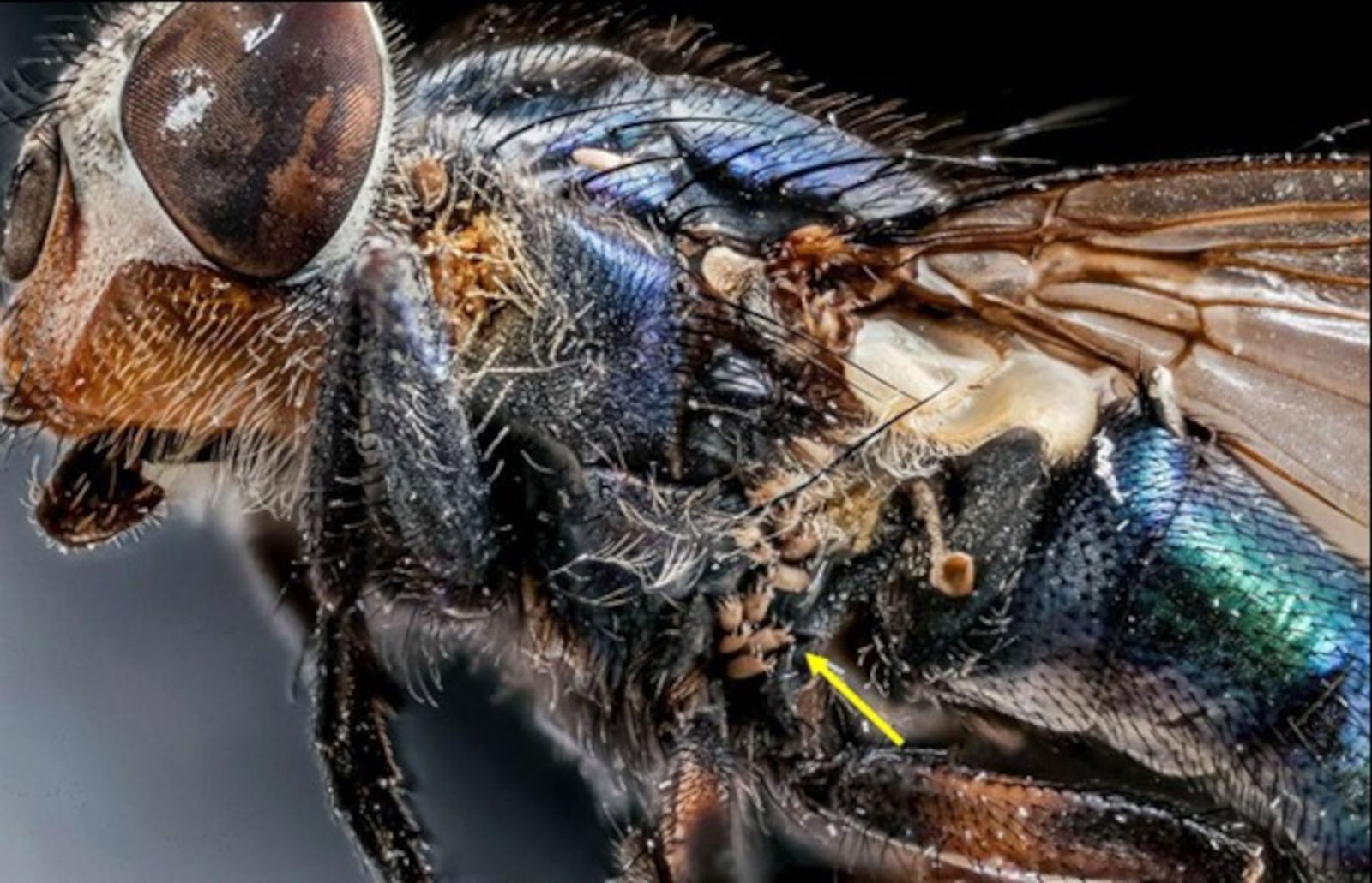
Figure 3. Deutonymphs of Myianoetus sp. (yellow arrow) between the thorax and abdomen of Compsomyiops fulvicrura.
Additionally, subsequent Fisher’s LSD analysis revealed statistically different groups among the study locations. A higher mean abundance of flies with attached mites was observed in Humahuaca, followed by Tumbaya and Tres Cruces (Table 3). It is noteworthy that the highest variance parameter for the dry season (-0.27) compared to the wet season (-0.09) suggests that these differences are primarily attributed to this time of the year, between June and August.

Discussion
The genus Myianoetus comprises more than 40 species widespread throughout the world (OConnor et al., 2015), most known only from deutonymphs phoretic on Diptera. In this work, the association between deutonymphs of Myianoetus sp. with C. fulvicrura is described for the first time. Up to present, there are reports of deutonymphs from the Myianoetus that have been found associated with various Diptera families: Sphaeroceridae (Fain et al., 1980), Muscidae (Centeno & Perotti, 1999; Greenberg & Carpenter 1960; Negm & Alatawi, 2011; Pimsler et al., 2016), Calliphoridae (Greenberg & Carpenter 1960; Miranda & Bermúdez, 2008) and Heleomyzidae (Zamec & Košel, 2014). Evidence obtained from lab experiments further described the phoretic interaction of the hypopi of Myianoetus muscarum with Muscina stabulans Fallen (Diptera: Muscidae), Stomoxys calcitrans Linnaeus (Diptera: Muscidae), Lucilia sericata (Diptera: Calliphoridae) and Musca domestica Linnaeus (Diptera: Muscidae) (Greenberg & Carpenter, 1960). Additionally, in a study carried out in Texas, USA, by Pimsler et al. (2016), a great number of M. muscarum individuals associated with Synthesiomyia nudiseta (Wulp) (Diptera: Muscidae) were collected in 3 human corpses.
Among the Calliphoridae species collected, C. albiceps stood out as the most abundant. However, deutonymphs of Myianoetus sp. were exclusively phoretically associated with C. fulvicrura. The statistical differences observed in the abundances of flies with attached mites among the different studied locations suggest that these were influenced by the dry season. Therefore, the preference for C. fulvicrura could be associated with seasonal variation, as it was more abundant during the dry season, contrasting with C. albiceps, which showed a preference for the wet season. These trends were notable in Tumbaya and Humahuaca, where C. albiceps was the dominant species, while in Tres Cruces, the abundance of this species was very low, with C. fulvicrura being the dominant species in both seasons in that area. Additionally, it is plausible that this choice is related to the chemical attraction of mites to volatile substances released by the puparia of C. fulvicrura, as demonstrated in the studies by Greenberg and Carpenter (1960). These observations were reflected in the prevalence values, which indicated higher values during the dry season in all 3 locations, compared to the wet season.

Figure 5. Dorsal view of Myianoetus sp. (scale = 0.05 mm). The yellow arrow indicates the hysterosomal setae (ex) and exobothridial setae (in).

Figure 6. Dorsal view of legs I and II of Myianoetus sp. (scale = 0.1 mm). The yellow arrow shows the bifurcate empodial claw, characteristic of the genus, present on legs I-III.

Figure 7. Abundance frequency (AF) histogram of Myianoetus sp. deutonymphs associated with Compsomyiops fulvicrura individuals.
The lack of interaction between Myianoetus sp. with other species and its demonstrated affinity with C. fulvicrura suggest that these mites can be phoretically selective in the Prepuna environment. At genus or species level, mites have micro-habitat specific requirements, being excellent specific environmental indicators, offering themselves as potentially one of the most informative pieces of biological trace evidence collected from a crime scene (Perotti & Braig, 2019). This may explain events of corpse location, of relocation, a link to a suspect and a possible connection between a suspect and a victim or a crime scene (Hani et al., 2018; Kamaruzaman et al., 2018; Szeleczl et al., 2018). The specificity and abundance of mites, coupled with the intensity of phoresy, could contribute to estimating more precise post-mortem intervals (PMI) (Miranda & Bermúdez, 2008; Rodrigueiro & Prado, 2004; Russell et al., 2004). In addition, Perotti and Braig (2009) suggested that the presence of a specific phoretic mite (for example Myianoetus sp.) may confirm the presence of its host (for example C. fulvicrura), even when the host is already gone.
Given that mites are a valuable forensic tool, it is crucial to deepen the understanding of the biology and ecology of the species involved. To expand this knowledge, it is necessary to continue registering and investigating new species and their phoretic associations under various climatic and biogeographical conditions.
Acknowledgements
We would like to thank Pablo A. Martínez for his critical analysis and recommendations for our manuscript, Mario A. Linares for the Myianoetus sp.photograph and Ismael Acosta for the C. fulvicrura photograph.
References
Arnaldos, M. I., García, M. D., Romera, E., Presa, J. J., & Luna, A. (2005). Estimation of post-mortem interval in real cases based on experimentally obtained entomological evidence. Forensic Science International, 149, 57–65. https://doi.org/10.1016/j.forsciint.2004.04.087
Barton, P. S., Weaver, H. J., & Manning, A. D. (2014). Contrasting diversity dynamics of phoretic mites and beetles associated with vertebrate carrion. Experimental and Applied Acarology, 63, 1–13. https://doi.org/10.1007/s10493-013-9758-7
Braig, H. R., & Perotti, M. A. (2009). Carcasses and mites. Experimental and Applied Acarology, 49, 45–84. https://doi.org/10.1007/s10493-009-9287-6
Bush, A. O., Lafferty, K. D., Lotz, J. M., & Shostak, A. W. (1997). Parasitology Meets Ecology on Its Own Terms: Margolis et al. Revisited. The Journal of Parasitology, 83, 575–583. https://doi.org/10.2307/3284227
Camerik, A. M. (2010). Phoresy revisited. In M. Sabelis, & J. Bruin (Eds.), Trends in Acarology (pp. 333–336). Dordrecht: Springer. https://doi.org/10.1007/978-90-481-9837-5_53
Catts, E. P., & Goff, M. L. (1992). Forensic entomology in criminal investigations. Annual Review of Entomology, 37, 253–272. https://doi.org/10.1146/annurev.en.37.010192.001345
Centeno, N. D., & Perotti, M. A. (1999). Ácaros vinculados a procesos de descomposición de cadáveres y sus posibles asociaciones foréticas. In Actas y Trabajos de la XIX Reunión Argentina de Ecología, 1999. Tucumán, Argentina.
Di Rienzo J. A., Casanoves, F., Balzarini, M. G., González, L., Tablada, M., & Robledo, C. W. (2020). InfoStat versión 2020. Centro de Transferencia InfoStat, FCA, Universidad Nacional de Córdoba, Argentina.
Dindal, D. L. (1990). Soil biology guide. New York: John Wiley and Sons.
Fain, A., Britt, D. P., & Molyneux, D. H. (1980). Myianoetus copromyzae sp. nov. (Acari, Astigmata, Anoetidae) phoretic on Copromyza atra (Meigen 1830) in Scotland. Journal of Natural History, 14, 401–403. https://doi.org/
10.1080/00222938000770341
Farish, D. J., & Axtell, R. C. (1971). Phoresy redefined and examined in Macrocheles muscaedomesticae (Acarina: Macrochelidae). Acarologia, 13, 16–29.
Greenberg, B., & Carpenter, P. D. (1960). Factors in phoretic association of a mite and fly. Science, 132, 738–739. https://doi.org/10.1126/science.132.3429.738
Hani, M., Thieven, U., & Perotti, M. A. (2018). Soil bulb mites as trace evidence for the location of buried money. Forensic Science International, 292, e25–e30. https://doi.org/10.1016/j.forsciint.2018.09.016
Heo, C. C., Teel, P. D., & OConnor, B. M. (2021). Acari community in association with delayed pig carrion decomposition. Experimental and Applied Acarology, 85, 223–246. https://doi.org/10.1007/s10493-021-00676-6
Hwang, C., & Turner, B. D. (2005). Spatial and temporal variability of necrophagous Diptera from urban to rural areas. Medical and Veterinary Entomology, 19, 379–391. https://doi.org/10.1111/j.1365-2915.2005.00583.x
Kamaruzaman, N. A. C., Mašán, P., Velásquez, Y., González-Medina, A., Lindström, A., Braig, H. R. et al. (2018). Macrocheles species (Acari: Macrochelidae) associated with human corpses in Europe. Experimental and Applied Acarology, 76, 453–471. https://doi.org/10.1007/s10493-018-0321-4
Margolis, L., Esch, G. W., Holmes, J. C., Kuris, A. M., & Schad, G. A. (1982). The use of ecological terms in parasitology (report of an ad hoc committee of the American Society of Parasitologists). Journal of Parasitology, 68, 131–133. https://doi.org/10.2307/3281335
Miranda, R., & Bermúdez, S. (2008). Ácaros (Arachnida: Acari) asociados con moscas Calliphoridae (Diptera: Oestroidea) en tres localidades de Panamá. Revista Colombiana de Entomología, 34, 192–196. https://doi.org/10.25100/socolen.v34i2.9287
Mulieri, P. R., Mariluis, J. C., & Patitucci, L. D. (2014). Calliphoridae. In S. Roig-Juñent, L. E. Claps, & J. J. Morrone (Eds.), Biodiversidad de artrópodos argentinos, Vol. 4 (pp. 463–474). INSUE, Universidad Nacional de Tucumán, San Miguel de Tucumán, Argentina.
Negm, M. W., & Alatawi, F. J. (2011). Four new records of mites (Acari: Astigmata) phoretic on insects in Riyadh, Saudi Arabia. Journal of the Saudi Society of Agricultural Sciences, 10, 95–99. https://doi.org/10.1016/j.jssas.2011.04.001
OConnor, B. M. (1982). Evolutionary ecology of astigmatid mites. Annual Review of Entomology, 27, 385–409. https://doi.org/10.1146/annurev.en.27.010182.002125
OConnor, B. M. (2009). Astigmatid mites (Acari: Sarcoptiformes) of forensic interest. Experimental and Applied Acarology, 49, 125–133. https://doi.org/10.1007/s10493-009-9270-2
OConnor, B. M., Pimsler, M. L., Owings, C. G., & Tomberlin, J. K. (2015). Redescription of Myianoetus muscarum (Acari: Histiostomatidae) associated with human remains in Texas, USA, with designation of a neotype from Western Europe. Journal of Medical. Entomology, 52, 539–550. https://doi.org/10.1093/jme/tjv045
Olea, S. M., & Mariluis, J. C. (2013). The genus Calliphora (Diptera: Calliphoridae) in Argentina, with the first records of C. lopesi Mello 1962. Revista de la Sociedad Entomológica Argentina, 72, 99–104.
Perotti, M. A., & Braig, H. R. (2009). Phoretic mites associated with animal and human decomposition. Experimental and Applied Acarology, 49, 85–124. https://doi.org/10.1007/s10493-009-9280-0
Perotti, M. A., Braig, H. R., & Goff, M. L. (2010). Phoretic mites and carcasses: Acari transported by organisms associated with animal and human decomposition. In J. Amendt, M. Goff, C. Campobasso, & M. Grassberger (Eds.), Current concepts in forensic Entomology (pp. 69–91). Dordrecht: Springer. https://doi.org/10.1007/978-1-4020-9684-6_5
Perotti, M. A., & Braig, H. R. (2019). Acarology in Crimino-Legal Investigations. In J. Byrd, & J. Tomberlin (Eds.), Forensic Entomology, 3rd. Edition (pp. 461–473). Boca Raton: CRC Press. https://doi.org/10.4324/9781351163767-22
Pimsler, M. L., Owings, C. G., Sanford, M. R., OConnor, B. M., Teel, P. D., Mohr, R. M., & Tomberlin, J. K. (2016). Associa-
tion of Myianoetus muscarum (Acari: Histiostomatidae) with Synthesiomyia nudiseta (Wulp) (Diptera: Muscidae) on human remains. Journal of Medical Entomology, 53, 290–295. https://doi.org/10.1093/jme/tjv203
Rai, J., Amendt, J., Bernhardt, V., Pasquerault, T., Lindström, A., & Perotti, M. A. (2020). Mites (Acari) as a relevant tool in trace evidence and postmortem analyses of buried corpses. Journal of Forensic Sciences, 65, 2174–2183. https://doi.org/10.1111/1556-4029.14506
Rodrigueiro, T. S. C., & Prado, A. P. (2004). Macrocheles muscaedomesticae (Acari, Macrochelidae) and a species of Uroseius (Acari, Polyaspididae) phoretic on Musca domestica (Diptera, Muscidae): effects on dispersal and colonization of poultry manure. Iheringia. Série Zoologia, 94, 181–185. https://doi.org/10.1590/S0073-47212004000200011
Russell, D. J., Schulz, M. M., & OConnor, B. M. (2004). Mass occurrence of astigmatid mites on human remains. Abhandlungen und Berichte des Naturkundmuseums Görlitz, 76, 51–56.
Saloña-Bordas, M. I., & Perotti, M. A. (2015). Acarología forense. Ciencia Forense, 12, 91–112.
Szelecz, I., Lösch, S., Seppey, C. V. W., Lara, E., Singer, D., Sorge, F. et al. (2018). Comparative analysis of bones, mites, soil chemistry, nematodes and soil micro-eukaryotes from a suspected homicide to estimate the post-mortem interval. Scientific Reports, 8, 25. https://doi.org/10.1038/s41598-017-18179-z
Whitworth, T. (2014). A revision of the Neotropical species of Lucilia Robineau- Desvoidy (Diptera: Calliphoridae). Zootaxa, 3810, 1–76. https://doi.org/10.11646/zootaxa.3810.
1.1
Zamec, R., & Košel, V. (2014). A new species of mite (Acari: Histiostomatidae) phoretic on Gymnomus caesius (Diptera: Heleomyzidae) from Vlčie Diery cave. Biologia, 69, 916–919. https://doi.org/10.2478/s11756-014-0387-3

Ringtails (Bassariscus astutus) as seed dispersers in an urban gradient under conditions of low human activity due to COVID-19
Joselin Judith Peña-Herrera a, Yury Glebskiy a, b, *, Teresa de Jesús Hernández-Trejo a, Zenón Cano-Santana a
a Universidad Nacional Autónoma de México, Facultad de Ciencias, Departamento de Ecología y Recursos Naturales, Laboratorio de Interacciones y Procesos Ecológicos, Circuito Exterior s/n, Ciudad Universitaria, Coyoacán, 04510 Ciudad de México, Mexico
b Universidad Nacional Autónoma de México, Facultad de Ciencias, Posgrado en Ciencias Biológicas, Circuito Exterior s/n, Ciudad Universitaria, Coyoacán, 04510 Ciudad de México, Mexico
*Corresponding author: agloti@ciencias.unam.mx (Y. Glebskiy)
Received: 14 September 2023; accepted: 6 March 2024
Abstract
Seed dispersal by animals is a key ecosystemic process in many environments; however, it could be compromised or increased in urban environments due to changes in the landscape, the introduction of exotic species, and human activities. This article aims to evaluate the role of ringtails (Bassariscus astutus) as seed dispersers in an urban-natural gradient during low human activity due to the COVID-19 pandemic. Ringtail feces were collected in 3 sampling sites with different levels of urbanization (ranging from 100 to 5% of natural vegetation), and the seeds germinated in germination chambers. Twenty species of plants were dispersed by ringtails, more than reported in previous studies. More seeds were dispersed in natural (7.1 seeds per g) than urbanized (3.2 seeds per g) areas, but diversity and richness were higher in urbanized areas. This suggests that urban environments have a greater diversity, and it could be attributed to the microenvironments created by urban infrastructure and the exotic plants that are established in the area.
Keywords: Endozoochory; Mexico City; Opuntia; REPSA; Zoochory
© 2024 Universidad Nacional Autónoma de México, Instituto de Biología. Este es un artículo Open Access bajo la licencia CC BY-NC-ND
(http://creativecommons.org/licenses/by-nc-nd/4.0/).
Cacomixtles (Bassariscus astutus) como dispersores de semillas en un gradiente urbano bajo condiciones de baja actividad humana por COVID-19
Resumen
La dispersión de semillas por animales es un proceso clave en muchos ecosistemas, pero este se puede ver comprometido o incrementado en ambientes urbanos debido a cambios en el paisaje, introducción de especies exóticas y actividades humanas. El objetivo de este artículo es evaluar el papel del cacomixtle (Bassariscus astutus) como dispersor de semillas en un gradiente urbano-natural durante un periodo de baja actividad humana debido a la pandemia de COVID-19. Se colectaron excretas de cacomixtles en 3 localidades con diferente grado de urbanización (entre 100 y 5% de vegetación natural) y las semillas fueron germinadas en cámaras de germinación. Se registraron 20 especies de plantas dispersadas, más que lo reportado en estudios previos. Más semillas fueron dispersadas en áreas naturales (7.1 semillas por g) que urbanizadas (3.2 semillas por g), pero la riqueza y diversidad fueron mayores en áreas urbanizadas. Ésto sugiere que la diversidad en ambientes urbanos es mayor, lo cual se puede atribuir a los microambientes formados por la infraestructura urbana y las plantas exóticas establecidas en el área.
Palabras clave: Endozoocoria; Ciudad de México; Opuntia; REPSA; Zoocoria
Introduction
Some animals may provide a key ecosystemic service, acting as seed dispersers, which allow many plant species to effectively move their offspring and maintain plant communities across different environments. An example of those animals is the ringtail (Procyonidae: Bassariscus astutus) which is an omnivorous and opportunistic animal that has shown potential to disperse the seeds of a great number of plant species across many ecosystems (Alexander et al., 1994; Rodríguez-Estrella et al., 2000; Rubalcava-Castillo et al., 2020). However, this important service could be diminished in urban ecosystems, where ringtails are very common (Barja & List, 2006; Swanson et al., 2022). Because urban areas offer new sources of food like anthropogenic waste and a variety of exotic plants, ringtails could disperse fewer seeds or seeds of exotic plants. This is an important concern since urban ecosystems are growing fast and thus becoming important areas for the conservation of species and areas on which we rely to obtain ecosystemic services.
Previous studies suggest that seed dispersal is diminished in cities due to a great number of unsuitable habitats (Cheptou et al., 2008) and barriers that obstruct animal movement and thus seed dispersal (Niu et al., 2018). However, animal-plant networks are persistent in cities (Cruz et al., 2013), and plants that rely on animal dispersal tend to have a more successful regeneration of populations than plants that rely on other strategies for dispersal (Niu et al., 2023). At the same time, most studies show that urban ecosystems tend to be more diverse than natural areas due to the great number of exotic species, microenvironments that can host greater plant diversity, and the fact that cities tend to be built in highly diverse locations (Kühn et al., 2004; Wania et al., 2006). Yet all these studies are performed in urban areas with both human activity and urban infrastructure; therefore, the hypothesis that urban areas are diverse due to the exotic plants and microhabitats and not due to “direct-human” seed dispersal (for example, seeds we throw away as garbage) is yet to be proven.
Particularly for the ringtails, Cisneros-Moreno and Martínez-Coronel (2019) found differences in the urban and rural ringtail diets. They report that in urban environments, ringtails consume 11 plant species, and 9 in rural environments. Other studies also show that ringtails commonly consume human-generated waste from trash cans when it is available (Castellanos et al., 2009; Picazo & García-Collazo, 2019). However, all those studies were made under normal human activity, but if it is reduced, the generation of waste could be diminished, affecting the ringtail diet, which in turn could lead to a change in their role as seed dispersers.
Therefore, this article aims to compare the diversity, abundance, and species of seeds dispersed by ringtails in 3 areas with different levels of urbanization during a time of reduced human activity due to the COVID-19 pandemic.
Materials and methods
This study was performed inside the main campus of the Universidad Nacional Autónoma de Mexico, located in Mexico City, Mexico. The campus contains a well-preserved ecological reserve (Reserva Ecológica del Pedregal de San Ángel; henceforth REPSA) and urban areas such as buildings and roads, all of which are surrounded by the Mexico City (Fig. 1). Therefore, a gradient between urban and natural areas can be found in a relatively small area (730 ha; Zambrano et al., 2016) that otherwise shares all environmental characteristics like mean temperature (18.2°C), precipitation (752 mm), original substrate, and vegetation: xerophitic shrubs (Rzedowski, 1954; SMN, 2023).
An important characteristic of this study is that it was performed under lockdown conditions due to the COVID-19 pandemic. Because of the rapid spreading of the virus, most activities on campus were switched to virtual mode; students took lessons from home; maintenance such as cleaning, gardening, and security were kept to a bare minimum; and all research activities had to be done from home, except for some specific cases, such as this study, that required special permission from the university. Those measures were implemented in March 2020 and began to be gradually lifted in the spring of 2022. Under normal conditions, the campus is visited by 166,474 people, and 70,000 vehicles, and 15 tons of waste (excluding gardening products) are generated (Zambrano et al., 2016). However, as a result of the pandemic, human activity on campus such as driving, waste generation and gardening, among others was minimal for 2 years. This gave us the opportunity to study the ringtail seed dispersal in an urban environment without human presence.
The correct identification of ringtail feces is an essential part of this project, since, in our study site, they could be confused with excretes of opossums (Didelphis virginiana). Previous studies suggest that opossums do not use latrines (Aranda, 2000), however, to ensure that latrines are used exclusively by ringtails, we placed camera traps in front of 8 latrines, and animal interactions with those latrines were recorded.

Figure 1. Map of the study location. Blue dots, Faculty (most urbanized area) latrines; red dots, the Institute latrines (semi-urban area); and green dots, the West core (natural area). The lines represent the 178 m around the latrines in which the percentages of the different types of terrain were calculated.
Three areas separated by at least 800 m were chosen to represent the urban-natural gradient: natural, semi-urban, and urban (Fig. 1). The home ranges of this species in the location are small: between 3 and 9.9 ha (Castellanos & List, 2005); therefore, this separation should ensure independence between the treatments. The level of urbanization was based on the percentage of area covered by natural vegetation, altered vegetation, impermeable areas without buildings (mainly roads and parking lots), and buildings found in a 178 m area (Fig. 1, Table 1) around the sampling points (178 m is the radius of the maximum activity area reported for ringtails in this particular location; Castellanos & List, 2005). The natural area (henceforth the West core) is located inside the west core of the REPSA. Vegetation consists mainly of shrubs, and Opuntia cactus is quite common (Cano-Santana, 1994). The semi-urban area (henceforth Institutes) is located around the humanitarian institutes area and consists of a mosaic of spatially located buildings, parking lots, altered vegetation (grass and some cultivated trees, mostly without fruit) and remnants of natural vegetation that surround this area on all sides (Fig. 1, Flores-Morales, 2023). The urban area (henceforth Faculty) is located inside the faculty of sciences and is dominated by tightly packed buildings divided by impermeable areas and gardens. The vegetation is diverse and includes a small amount of native plants such as Opuntia, but mostly consists of grass and introduced trees some of which have fruits that could be consumed by ringtails (Mendoza-Hernández & Cano-Santana, 2009). During the lockdown, gardens were left mostly unattended, and some alimentary plants began to grow (for example, we encountered several tomato plants with ripe fruits). The natural vegetation is located mostly on the edges of this area (Fig. 1).
Table 1
Amount of terrain coverage in the sampling areas. Impermeable areas were considered all areas covered with concrete but without buildings, mainly roads and parking lots.
| Natural vegetation (%) | Altered vegetation (%) | Buildings (%) | Impermeable areas (%) | Total area (ha) | |
| West core | 100 | 0 | 0 | 0 | 34.1 ha |
| Institutes | 49.2 | 24.2 | 7 | 19.6 | 30.7 ha |
| Faculty | 4.9 | 35 | 30.5 | 29.6 | 15.4 ha |
To estimate the number of seeds dispersed by ringtails, we collected excretes from 13 latrines in each location, on January 18th 2022. Since previous studies report that seeds in our study area commonly have dormancy (Glebskiy, 2019), half of each latrine excretes was placed in plastic bags and half in mesh bags (with 1 × 1 mm openings). Both treatments were left in the field (on the soil and without cover) until April 29th 2022 (when the rains and thus the germination period started). The advantage of the plastic bag treatment is that it allows the seeds to experience the temperature changes that are responsible for ending dormancy in most plants and protects the seeds, but limits some other factors like gas exchange and humidity that could potentially contribute to the end of dormancy (Baskin & Baskin, 1998). On the other hand, the mesh bag allows for a better representation of the natural conditions to which seeds are exposed but is susceptible to losing seeds through the mesh and the addition of new seeds from the environment. Both methods were tested.
At the beginning of the rainy season (April 29th 2022) bags were collected and put to germinate in commercial soil (the soil was sterilized by microwaving, and a control with no excretes was used to test the efficiency of sterilization and possible future seed additions) in a germination chamber (25°C, 16 hours of light, and 8 hours of darkness) for 4 months. All plant germinations were recorded and identified to morphospecies; when the plants grew, they were identified to the finest level possible. Species that germinated in the control pot were considered later additions and excluded from the analysis.
Data were analyzed with the R statistical packages: stats (R core team, 2022), dunn.test (Dinno, 2017), fossil (Vavrec, 2011), and vegan (Oksanen et al., 2022). Number of germinated seeds per gram of excrete was calculated. To compare between treatments (3 locations and 2 types of protection bags) Kruskal-Wallis and Dunn tests were performed for the total number of germinated seeds and the number of Opuntia seeds (this was the only species with enough data to analyze independently). A GLIM test (with Poisson distribution) was used to determine if the level of protection (plastic bags = 1, mesh bags = 0) and amount of vegetation (both natural and altered) influenced the amount of total and Opuntia germinated seeds. To compare the richness and diversity of dispersed seeds, we calculated the Shannon diversity and Chao 1 (± 95% confidence interval) richness. The similarity between treatments was measured using the Jaccard and Bray-Curtis indexes.
Results
A total effort of 329 trap nights was performed with 199 independent records (at least 1 hour between sightings) of ringtails, of which 44 times ringtails defecated in the latrine (Fig. 2). Opossums were observed 66 times, and no defecation was observed. At the same time, there were 9 observations of rodents and 7 of birds feeding from the latrines.
A total of 52 bags were recovered from the field (34 plastic, and 18 mesh bags), and were put to germinate. In total, 782 plants of 20 species (Table 2) germinated in this experiment. More seeds per gram of excrete germinated in the mesh bags treatment (U tests; V = 1,225, p < 0.001); however, more Opuntia seeds germinated in the plastic bag treatment (U test; V = 300, p < 0.001; Table 3). The Kruskal-Wallis test showed no differences in the number of germinated seeds between locations in the mesh bags, but there were significant differences for total seed and Opuntia seeds in the plastic bag treatment (p = 0.042 and p = 0.002). According to the Dunn test, there were fewer total seeds in the Faculty area than the West core (p = 0.009) and fewer Opuntia seeds in the Faculty area than the Institutes (p = 0.015) and the West core (p = 0.009).
GLIM analysis showed that both level of protection (-0.818, p < 0.001) and vegetation area (1.279, p < 0.001) are significant predictors for the number of total seeds germinated. For Opuntia seeds, protection (1.674, p < 0.001) and vegetation (3.559, p < 0.001).

Figure 2. a) Ringtail defecating in a latrine; b) a rodent consuming seeds from a latrine; c) a latrine; d) plants germinated from excretes.
We found significant differences in richness (according to Chao1) between the Faculty area and the West core (in plastic bags) and between the Faculty area and Institutes and the West core (in mesh bags; Table 4). The Bray-Curtis dendrogram shows 2 important groups: the mesh bag treatment and the plastic bag (Fig. 3). Jaccard index showed the following results within the same location,Faculty plastic-Faculty mesh: 0.714, Institutes plastic-Institutes mesh: 0.546, West core plastic-West core mesh: 0.571, total plastic-total mesh: 0.65; between locations,plastic bags, Faculty plastic-Institutes plastic: 0.769, Faculty plastic-West core plastic: 0.5, Institutes plastic-West core plastic: 0.643;between locations, mesh bags, Faculty mesh-Institutes mesh: 0.5, Faculty mesh-West core mesh: 0.294, Institutes mesh-West core mesh: 0.333.

Figure 3. Bray-Curtis dendrogram of germination treatments. First letter represents the location, W: west core, I: Institutes, F: Faculty; second letter, the type of bag: M: mesh, P: plastic.
Discussion
The camera trap experiment was designed to prove that the latrines from which we collected excretes belong to ringtails and not opossums since those animals produce very similar feces (Aranda, 2000). Given that we observed 44 events of defecation by ringtails and zero by opossums, it we can conclude that ringtails are the only latrine users. However, at the same time, rodents and birds were seen feeding in those latrines (Fig. 2). The ratio for those visits is 1 visit per 2.8 defecations, and this is important for seed dispersal, since most likely those visitors feed on seeds that are dropped by ringtails and can selectively remove some species. At the same time, it is interesting to consider the trade-off for the rodents that consume seeds from ringtail latrines since they are exposed to predation by the latrine owners. Although it is outside the scope of this research, we consider that the interaction around the latrines is a topic that should be further investigated to better understand the role of these animals as seed dispersers and the interactions that the latrines produce.
The comparison between plastic and mesh bags shows differences between the treatments, especially in the number of seeds that germinated per gram of excrete (Tables 2, 3). This could be attributed to the fact that mesh bags allow the smallest particles to exit the bag, and the total weight of feces diminishes while the number of seeds remains constant. Therefore, the mesh bag treatment is not adequate for estimating the number of seeds per gram of excrete, although data concerning the diversity and richness of seeds is still valid. Given the above and the fact that there were more plastic bag replicas, the data interpretation in this research is based on the plastic bag treatment.
Table 2
Number of seeds per gram of excrete in all treatments for each plant species.
| Species | Common name | Faculty | Institutes | West core | |||
| Plastic | Mesh | Plastic | Mesh | Plastic | Mesh | ||
| Ageratina sp. 1 | Snakeroot | 0.11 | 3.19 | 0.41 | 2.95 | 0.12 | 8.63 |
| Ageratina sp. 2 | Snakeroot | 0.02 | 0.09 | 0.02 | 0 | 0 | 0 |
| Asclepias linaria | Pineneedle milkweed | 0 | 0 | 0 | 0 | 0.13 | 0 |
| Amaranthaceae | 0.33 | 0.19 | 0 | 0 | 0 | 0 | |
| Bidens sp. | Beggarticks | 0 | 0 | 0.02 | 0 | 0.05 | 0.61 |
| Cissus sicyoides | Princess vine | 0 | 0 | 0 | 0 | 0.03 | 0.33 |
| Conyza sp. | Horseweed | 0.07 | 0.22 | 0.26 | 0 | 0 | 0 |
| Drymaria laxiflora | Chickweed | 0.04 | 0.27 | 0.12 | 0.35 | 0.03 | 2.68 |
| Eragrostis sp. | Lovegrass | 0 | 0.09 | 0 | 0 | 0 | 0 |
| Iresine sp. | Bloodleaf | 0 | 0 | 0 | 0 | 0 | 2.04 |
| Opuntia sp. | Prickly pear | 0.23 | 0.98 | 2.23 | 0.59 | 6.36 | 0.24 |
| Solanaceae | 0.03 | 0.27 | 0.08 | 0 | 0.1 | 0.71 | |
| Solanum nigrescens | Slender nightshade | 0.1 | 2.79 | 0.04 | 2.14 | 0.08 | 0 |
| Stevia sp. | Stevia | 0 | 0.09 | 0 | 0 | 0 | 0 |
| Phytolacca icosandra | Tropical pokeweed | 0.46 | 0.15 | 0.25 | 0.22 | 0.08 | 0 |
| Poaceae 1 | 0.02 | 0.39 | 0.12 | 0.07 | 0.13 | 0.17 | |
| Poaceae 2 | 0 | 0 | 0 | 0 | 0 | 0.25 | |
| Unknown sp. 1 | 0.02 | 0 | 0.1 | 0 | 0.05 | 0.33 | |
| Unknown sp. 2 | 0 | 0 | 0 | 0 | 0.05 | 0 | |
| Unknown sp. 3 | 1.72 | 0 | 0 | 0 | 0 | 0 |
Table 3.
Number of Opuntia and total seeds dispersed by ringtails in different environments. Values given in seeds per g of excrete ± S.D.
| Total seeds | Opuntia seeds | |||
| Plastic | Mesh | Plastic | Mesh | |
| West core | 7.13 ± 8.06 | 15.99 ± 13.85 | 6.36 ± 7.58 | 0.24 ± 0.3 |
| Institutes | 3.64 ± 2.87 | 6.33 ± 6.61 | 2.23 ± 2.72 | 0.59 ± 1.33 |
| Faculty | 3.16 ± 7.09 | 8.72 ± 5.51 | 0.23 ± 0.75 | 0.98 ± 2.39 |
| Total | 4.7 ± 6.64 | 10.88 ± 10.26 | 2.96 ± 5.46 | 0.58 ± 1.5 |
GLIM analysis shows a positive relation between the number of seeds dispersed by ringtails and vegetation cover. Therefore, ringtails disperse fewer seeds in urban areas (Table 3); however, diversity and richness tend to be higher in the Faculty, the most urbanized location (Table 4).
Table 4
Richness (Chao1 ± 95% confidence intervals) and diversity (Shannon) of seeds dispersed by ringtails.
| Faculty | Institutes | West core | Total | |||||||||
| Plastic | Mesh | Total | Plastic | Mesh | Total | Plastic | Mesh | Total | Plastic | Mesh | Total | |
| Observed richness | 12 | 12 | 14 | 11 | 6 | 11 | 12 | 10 | 14 | 16 | 17 | 20 |
| Chao1 | 16 ± 2.65 | 14.67 ± 1.85 | 18.5 ± 3.9 | 15 ± 2.65 | 8 ± 1.87 | 17 ± 0 | 12.17 ± 0.34 | 10.25 ± 0.44 | 14.5 ± 0.73 | 16.25 ± 0.44 | 19.67 ± 1.85 | 24.5 ± 3.4 |
| Shannon | 1.45 | 1.839 | 1.889 | 1.273 | 1.434 | 1.466 | 0.564 | 1.758 | 1.122 | 1.403 | 2.041 | 1.779 |
This is consistent with most previous studies that show a greater diversity of seeds in urban settings (Kühn et al., 2004; Wania et al., 2005), and that ringtails consume more plant species in the cities (Cisneros-Moreno & Martínez-Coronel, 2019). At our location, ringtails disperse fewer seeds in urban areas, but their richness and diversity are higher. The novel contribution of this research is that it was performed in an urban area with very little human activity; therefore, the direct effect of human activities such as waste generation and gardening could not explain the differences between treatments. At the same time, all 3 locations share very similar climatic conditions and originally were the same ecosystem. This suggests that differences between treatments are not due to original conditions (although it has been proven in other locations; Kühn et al., 2004). The high diversity of seeds in urbanized areas can be attributed to the great variety of habitats found in an urban area and the exotic species that have already been established there.
Ringtails are common in urban areas, and Castellanos et al. (2009) suggest they prefer disturbed areas over natural ones. This could be due to food availability in urbanized areas, and previous studies show that ringtails have a greater variety of food in urban areas. For example, Cisneros-Moreno and Martínez-Coronel (2019) show that an urban population consumes 36 food items and a rural population registered 28 items. Another advantage that cities offer is infrastructure. Poglayen-Neuwall and Toweill (1988) mention that rocky habitats favor ringtails, and human-made buildings provide a similar habitat. Interestingly, some data suggests that in the absence of humans, sightings of those animals in urban areas increased (Tzintzun-Sánchez, 2022; pers. obs.). This suggests that the benefits ringtails obtain from cities don’t come directly from human activities since, even without our presence, those animals have the benefits of infrastructure and a more diverse diet. However, further studies are needed to fully prove this hypothesis.
Previous studies have reported that fruits are important in the diet of B. astutus; however, the number of different plant species is generally low (13, ~ 9, 10, Alexander et al. [1994], Harrison [2012], and Rodríguez-Estrella et al. [2000], accordingly). In this study, 20 species of seeds were found and it is noteworthy that the cited articles included all vegetal matter in their analysis while this study only considers seeds that germinated. This suggests that the diversity of plants that are consumed in our site is much higher than usual. This could be the result of higher plant diversity in the location, or that ringtails tend to have a more frugivore diet here, this last hypothesis is supported by personal observations of the authors.
Based on the above, it could be concluded that there are several animals that consume the latrine contents, and this interaction could be important for seed dispersal. Ringtails disperse more seeds in natural areas, but their richness is higher in urban areas even in the absence of human activity.
Acknowledgements
We are thankful to M. E. Muñiz-Díaz for facilitating the germination chambers and her advice during this research, to Y. Martínez-Orea for helping with plant identification, to I. Castellanos-Vargas for technical support, and to the SEREPSA working team for facilitating the permission to perform this research. This project was financially supported by PAPIIT grant IN212121 (“El efecto de la urbanización sobre el tlacuache Didelphis virginiana en un matorral xerófilo de la Ciudad de México”), awarded to ZCS.
References
Alexander, L. F., Verts, B. J., & Farrell, T. P. (1994). Diet of ringtails (Bassariscus astutus) in Oregon. Northwestern Naturalist, 75, 97–101. https://doi.org/10.2307/353683131
Aranda, M. (2000). Huellas y otros rastros de los mamíferos grandes y medianos de México. Cuernavaca, Morelos: Instituto de Ecología, A.C./ la Comisión Nacional para el conocimiento y Uso de la Biodiversidad.
Barja, I., & List, R. (2006). Faecal marking behaviour in ringtails (Bassariscus astutus) during the non-breeding period: spatial characteristics of latrines and single faeces. Chemoecology, 16, 219–222. https://doi.org/10.1007/s00049-
006-0352-x
Baskin, C. C., & Baskin, J. M. (1998). Seeds: ecology, biogeography, and, evolution of dormancy and germination. San Diego: Academic Press.
Cano-Santana, Z. (1994). Flujo de energía a través de Sphenarium purpuracens (Orthoptera: Acrididae) y productividad primaria neta aérea en una comunidad xerófila (Ph.D. Thesis). Facultad de Ciencias, Universidad Nacional Autónoma de México. México D.F.
Castellanos, G., García, N., & List, R. (2009). Ecología del cacomixtle (Bassariscus astutus) y la zorra gris (Urocyon cinereoargenteus). In A. Lot, & Z. Cano (Eds.), Biodiversidad del ecosistema del Pedregal de San Ángel (pp. 371–381). Ciudad de Mexico: Secretaria Ejecutiva de la REPSA-UNAM.
Castellanos, G., & List, R. (2005). Área de actividad y uso de hábitat del cacomixtle (Bassariscus astutus) en “El Pedregal de San Ángel”. Revista Mexicana de Mastozoología, 9, 113–122.
Cheptou, P. O., Carrue, O., Rouifed, S., & Cantarel, A. (2008). Rapid evolution of seed dispersal in an urban environment in the weed Crepis sancta. Proceedings of the National Academy of Sciences, 105, 3796–3799. https://doi.org/10.1073/pnas.0708446105
Cisneros-Moreno, C., & Martínez-Coronel, M. (2019). Alimentación del cacomixtle (Bassariscus astutus) en un ambiente urbano y uno agrícola en los valles centrales de Oaxaca. Revista Mexicana de Mastozoología (Nueva Época), 9, 31–43. https://doi.org/10.22201/ie.20074484e.2019.1.1.274
Cruz, J. C., Ramos, J. A., Da Silva, L. P., Tenreiro, P. Q., & Heleno, R. H. (2013). Seed dispersal networks in an urban novel ecosystem. European journal of forest research, 132, 887–897. https://doi.org/10.1007/s10342-013-0722-1
Dinno, A. (2017). dunn.test: Dunn’s Test of Multiple Comparisons Using Rank Sums. R package version 1.3.5, https://CRAN.R-project.org/package=dunn.test
Flores-Morales, I. (2023). Diversidad vegetal y animal de los pedregales remanentes de la Zona de Institutos de Investigaciones en Humanidades de Ciudad Universitaria, Ciudad de México, México (Bachelor’s Thesis). Facultad de Ciencias, UNAM. Mexico City.
Glebskiy, Y. (2019). Efecto del conejo castellano (Sylvilagus floridanus) sobre la comunidad vegetal del Pedregal de San Ángel. (M. Sc. Thesis). Facultad de Ciencias, UNAM. México City.
Harrison, R. L. (2012). Ringtail (Bassariscus astutus) ecology and behavior in central New Mexico, USA. Western North American Naturalist, 72, 495–506. https://doi.org/
10.3398/064.072.0407
Kühn, I., Brandl, R., & Klotz, S. (2004). The flora of German cities is naturally species rich. Evolutionary Ecology Research, 6, 749–764.
Mendoza-Hernández, P. E., & Cano-Santana, Z. (2009). Elementos para la restauración ecológica de pedregales: la rehabilitación de áreas verdes de la Facultad de Ciencias en Ciudad Universitaria. In A. Lot, & Z. Cano-Santana (Eds.), Biodiversidad del ecosistema del Pedregal de San Ángel (pp. 523–532). Ciudad de México: Secretaría Ejecutiva de la REPSA-UNAM.
Niu, H., Rehling, F., Chen, Z., Yue, X., Zhao, H., Wang, X. et al. (2023). Regeneration of urban forests as influenced by fragmentation, seed dispersal mode and the legacy effect of reforestation interventions. Landscape and Urban Planning, 233, 104712. https://doi.org/10.1016/j.landurbplan.2023.104712
Niu, H. Y., Xing, J. J., Zhang, H. M., Wang, D., & Wang, X. R. (2018). Roads limit of seed dispersal and seedling recruitment of Quercus chenii in an urban hillside forest. Urban Forestry & Urban Greening, 30, 307–314. https://doi.org/10.1016/j.ufug.2018.01.023
Oksanen, J., Simpson, G., Blanchet, F., Kindt, R., Legendre, P., Minchin, P. et al. (2022). vegan: Community Ecology Package. R package version 2.6-2, https://CRAN.R-project.org/package=vegan
Picazo, G. E. R. C., & García-Collazo, R. (2019). Comparación de la dieta del cacomixtle norteño, Bassariscus astutus de un bosque templado y un matorral xerófilo, del centro de México. Biocyt: Biología, Ciencia y Tecnología, 12, 834–845. https://doi.org/10.22201/fesi.20072082.2019.12.68527
Poglayen-Neuwall, I., & Toweill, D. E. (1988). Bassariscus astutus. Mammalian Species, 327, 1–8.
R Core Team (2022). R: a language and environment for statistical computing. R Foundation for Statistical Computing, Vienna, Austria. https://www.R-project.org/
Rodríguez-Estrella, R., Moreno, A. R., & Tam, K. G. (2000). Spring diet of the endemic ring-tailed cat (Bassariscus astutus insulicola) population on an island in the Gulf of California, Mexico. Journal of Arid Environments, 44, 241–246. https://doi.org/10.1006/jare.1999.0579
Rubalcava-Castillo, F. A., Sosa-Ramírez, J., Luna-Ruíz, J. J., Valdivia-Flores, A. G., Díaz-Núñez, V., & Íñiguez-Dávalos, L. I. (2020). Endozoochorous dispersal of forest seeds by carnivorous mammals in Sierra Fría, Aguascalientes, Mexico. Ecology and Evolution, 10, 2991-3003. https://doi.org/10.1002/ece3.6113
Rzedowski, J. (1954). Vegetation of Pedregal de San Ángel. Anales de la Escuela Nacional de Ciencias Biológicas, IPN, Mexico, 8, 59 Endozoochorous 129.
SMN (Servicio Meteorológico Nacional). (2023). Normales climatológicas de la estación 00009071 Colonia Educacion (1991-2020). Consulted on 12 September 2023. https://smn.conagua.gob.mx/tools/RESOURCES/Normales_Climatologicas/Normales9120/df/nor9120_09071.TXT
Swanson, A. C., Conn, A., Swanson, J. J., & Brooks, D. M. (2022). Record of an Urban Ringtail (Bassariscus astutus) Outside of its Typical Geographic Range. Urban Naturalist Notes, 9, 1–6.
Tzintzun-Sánchez, C. L. (2022). Efectos de la urbanización en la distribución geográfica y hábitos alimenticios del cacomixtle norteño (Bassariscus astutus) en la Ciudad de México, México (Bachelor’s Thesis). Facultad de Ciencias, UNAM. Ciudad de México.
Vavrek, M. J. (2011). fossil: palaeoecological and palae-
ogeographical analysis tools. Palaeontologia Electronica, 14:1T. http://palaeo-electronica.org/2011_1/238/index.html
Wania, A., Kühn, I., & Klotz, S. (2006). Plant richness patterns in agricultural and urban landscapes in Central Germany —spatial gradients of species richness. Landscape and Urban planning, 75, 97–110. https://doi.org/10.1016/j.landurbplan.
2004.12.006
Zambrano, L., Rodríguez-Palcios, S., Pérez-Escobedo, M., Gil-Alarcón, G. Camarena, P., & Lot, A. (2016). Reserva Ecológica del Pedregal de San Ángel: atlas de riesgos. Ciudad de Mexico: Secretaría Ejecutiva de la REPSA-UNAM.

Don’t count your eggs before they hatch: differential survival of artificial bird nests in an anthropogenically modified landscape in western Mexico
Dallas R. Levey a, b, Ian MacGregor-Fors c, *
a Stanford University, Department of Biology, 327 Campus Drive, Stanford, California, 94305 USA
b Universidad Nacional Autónoma de México, Instituto de Biología, Tercer Circuito s/n, Ciudad Universitaria, Coyoacán, 04510 Mexico City, Mexico
c University of Helsinki, Faculty of Biological and Environmental Sciences, Ecosystems and Environment Research Programme, Niemenkatu 73, FI-15140, Lahti, Finland
*Corresponding author: ian.macgregor@helsinki.fi (I. MacGregor-Fors)
Received: 19 October 2023; accepted: 1 February 2024
Abstract
Native habitat conversion to urban and agricultural areas represents conservation concerns for habitat quality and the breeding success of birds. In tropical areas facing regular deforestation of at-risk habitats, changes may occur to bird and nest predator communities that influence contradictory trends in breeding success. To assess the value of working lands for birds, we placed 100 artificial nests in 5 habitat types of varying human footprint, including a tropical dry forest reserve, a biological research station, croplands, and 2 urban towns. We report a clear decline in survival from the forest to urban towns. Habitat type explained the variation in nest survival probabilities over nest height, elevation, or time of nest exposure. Reducing the structural and compositional contrast of habitat and landscape vegetation between tropical dry forest and working lands represent valuable conservation actions for increasing habitat quality for birds.
Keywords: Croplands; Bird nest predation; Habitat quality; Jalisco; Plasticine eggs; Tropical dry forest; Urbanization
© 2024 Universidad Nacional Autónoma de México, Instituto de Biología. Este es un artículo Open Access bajo la licencia CC BY-NC-ND
(http://creativecommons.org/licenses/by-nc-nd/4.0/).
No cuentes los huevos antes de que eclosionen: supervivencia diferencial de nidos artificiales de aves en un paisaje antropogénicamente modificado en el oeste de México
Resumen
La conversión de hábitats nativos en áreas urbanas y campos agrícolas representa problemas de conservación para la calidad del hábitat y el éxito reproductivo de las aves. La deforestación constante de hábitats en riesgo puede cambiar las comunidades de aves y los depredadores de los nidos, lo que puede influir en su éxito reproductivo. Para evaluar el valor de los hábitats dentro de un paisaje antropogénicamente modificado en el éxito reproductivo de las aves, colocamos 100 nidos artificiales en 5 hábitats con diferentes niveles de actividades humanas, incluyendo una reserva de bosque tropical caducifolio, una estación de investigación biológica, campos agrícolas y 2 pueblos urbanos. Encontramos una clara disminución en la supervivencia de nidos artificiales desde el bosque tropical caducifolio hasta los pueblos urbanos. El tipo de hábitat fue la variable que mejor explicó la variación en las probabilidades de supervivencia de los nidos artificiales en comparación con la altura del nido, la elevación y el tiempo de exposición del nido. Reducir el contraste dentro del paisaje en la estructura de la vegetación entre la reserva y los hábitats dentro del paisaje modificado representan acciones de conservación importantes para aumentar la calidad del hábitat para las aves.
Palabras clave: Campos agrícolas; Depredación de nidos de aves; Calidad de hábitat; Jalisco; Huevos de plastilina; Selva seca tropical; Urbanización
Introduction
Urbanization and the conversion of native habitat to agricultural land represent key factors in the long-term conservation of bird biodiversity (Aronson et al., 2014; Kehoe et al., 2017). In the tropics, urbanization and agriculture have led to the degradation and destruction of native vegetation and the reconfiguration of landscapes, causing stark contrast in habitat complexity between remnant vegetation and agricultural and urban areas that pose risks to bird biodiversity (Filloy et al., 2019; Fischer et al., 2015; Maas et al., 2016). Biodiverse tropical regions suffer some of the highest rates of urbanization and native habitat transformation (Estrada et al., 2020), which represent pressing challenges for the conservation of bird populations.
A key component of bird biodiversity and population monitoring in tropical landscapes with high rates of natural habitat transformation includes the evaluation of breeding ecology (DeGregorio et al., 2016). Reduced vegetative complexity and the exchange of native plants with non-native plants, both common attributes of agricultural and urban areas (Chace & Walsh, 2006), tend to negatively impact bird species with highly sensitive breeding requirements tied to native vegetation (Maas et al., 2016). Vegetation change in the tropics alters biotic —e.g., nest predation pressure and reduction of nest locations— and abiotic conditions —e.g., increased nest exposure, higher temperatures, and brighter conditions—, leading to potential direct and indirect influences on avian breeding ecology in species that depend on native plants and vegetation structure for nesting (Estrada et al., 2002; Rivera-López & MacGregor-Fors, 2016; Tellería & Díaz, 1995; Zuñiga-Palacios et al., 2021). Meanwhile, certain bird species may be positively impacted by or able to acclimate to novel conditions (DeGregorio et al., 2016; Kurucz et al., 2021; Latif et al., 2012), underlining the semi-permeable ecological filter that is applied to nesting birds in human-modified tropical landscapes and the importance of evaluating bird breeding ecology in different types of transformed land (MacGregor-Fors, 2010; MacGregor-Fors et al., 2022).
Nest predation represents a powerful force on bird breeding success and population dynamics (DeGregorio et al., 2016). A consequence of native habitat conversion to more urban or agricultural areas includes changes to nest predator communities, and the ability of bird species to adapt to these changes will ultimately determine whether disturbed areas offer viable habitat for native levels of biodiversity (DeGregorio et al., 2016; Latif et al., 2012). Urban and agricultural areas tend to have lower vegetation cover as forested habitats, leading to different natural predator abundance and nest visibility to predators, representing powerful determinants of breeding success for bird species that use transformed land (López-Flores et al., 2009; Martin, 1993; Zuñiga-Palacios et al., 2021). More disturbed areas may lead to a reduction of nest predation pressure due to the absence of native nest predators that have a low tolerance for human activity (Kurucz et al., 2021; Pretelli et al., 2023). A possible caveat to lower predation pressure from typical native predators in urban areas include birds that are habitat and foraging generalists (Estrada et al., 2002; Martin, 1995; Rivera-López & MacGregor-Fors, 2016), mammals that are attracted to anthropogenic food sources (Fischer et al., 2012), and increased access to nests by people that manipulate and destroy nests and eggs (López-Flores et al., 2009).
To assess the survivorship of bird nests, we placed artificial bird nests in 5 habitat types with increasing degrees of human disturbance and habitat modification, including 1) a tropical dry forest reserve (TDF hereafter), 2) the Chamela Biological Research Station (CBRS) grounds, embedded in the Chamela-Cuixmala Biosphere Reserve, 3) croplands (CL), 4) Careyes (CAR), a small and heavily built-up town, and 5) Emiliano-Zapata (ZAP), a larger town. While a recent meta-analysis questions the efficacy of artificial nest studies in determining nest survival probabilities in urban areas relative to natural nests (Vincze et al., 2017), the feasibility of finding sufficient numbers of natural nests in heavily built-up urban areas (i.e., outside of urban parks and green spaces) makes the use of artificial nests necessary. We controlled for important variables that may influence predation rates, such as nest size and height, to focus on habitat-level variations in nest survivorship and the impacts of urban and agricultural areas in the working landscape. Such landscapes are common in the tropical areas of Mexico (Levey et al., 2023), where existing reserves are surrounded by a working landscape with non-native vegetation that contrasts highly with native areas (Levey & MacGregor-Fors, 2021; Levey et al., 2021; MacGregor-Fors & Schondube, 2011; Vázquez-Reyes et al., 2017). Efforts to evaluate the impacts on breeding ecology in these working tropical landscapes are needed to supplement a thin body of work (Estrada et al., 2002; López-Flores et al., 2009; Zuñiga-Palacios et al., 2021) and determine the risks that urban and agricultural areas present for breeding birds. We expected nest survivorship to be lower in CL, CAR, and ZAP relative to the conserved TDF reserve and the CBRS due to higher exposure of nests and greater visibility for predators due to reduced vegetation complexity and density (Estrada et al., 2002; López-Flores et al., 2009; Zuñiga-Palacios et al., 2021).
Materials and methods
We conducted our study in a landscape between the Chamela-Cuixmala Biosphere Reserve (19°29’57.5” N, 105°02’41.6” W) and the town Emiliano Zapata (19°23’16.6” N, 104°57’50.1” W) in the Municipality La Huerta (population: 23,258; INEGI, 2020) on the Pacific coast of Jalisco, Mexico (Fig. 1). Historically, native vegetation cover in the region consisted primarily of tropical dry forest, which consists of deciduous forest with a mean canopy height of 12 m, a dense understory (Rzedowski, 2006), and strong phenological changes due to highly seasonal rainfall in the region (Durán et al., 2002). Other forest types exist in areas with more regular water availability, including semi-deciduous (mean canopy height of 20 m) and mangrove forests (Durán et al., 2002). After a period of increased human occupation and agricultural expansion from 1950-1970, large cover of tropical dry forest and other native forest types in lower elevation zones were converted to small towns and agricultural lands, linked by paved and unpaved roads, creating a landscape mosaic of native and non-native vegetation types (Maass et al., 2005).
In this landscape, we selected 5 habitat types with varying degrees of urban and agricultural disturbance for artificial nest placement: 1) TDF, with closed canopy cover and dense understory, 2) CBRS, which consists of moderately built-up 1.4 ha area embedded within the Chamela-Cuixmala Biosphere Reserve, 3) CL, consisting of fields of small, herbaceous plants such as maize (Zea mays), squash (Cucurbita spp.), chili pepper (Capsicum spp.), watermelon (Citrullus lanatus), and beans (Phaseolus spp.) located in the southern edge of the study area (Maass et al., 2005), 4) CAR (19°26’36.15” N, 105°1’49.65” W), a small town with heavy built-up cover, and 5) ZAP, a large town with less built-up cover than CAR (Fig. 1). Both elevations (MSL) of the TDF and CBRS sampling areas were slightly higher than the other habitat types. The TDF and CBRS sampling areas are also in closer proximity to each other than the other sampling locations. We included both habitat categories due to the higher human presence at the Biological Station, the noise generated by people and activities at the station, and a higher density of paved roads that could influence the occupancy of bird and mammals that respond positively to increasing human footprint (Rivera-López & MacGregor-Fors, 2016). Potential bird nest predators in the study region included White-throated Magpie-jays and San Blas jays (Calocitta formosa and Cyanocorax sanblasianus), Great-tailed grackles (Quiscalus mexicanus), mammals (e.g., Nasua narica, domestic dogs and cats, rodents, possums, and Procyon lotor), and diverse reptiles.
We used a mixture of plant fibers, twigs, and mud from the nest location to create bird nests in the shape of open plant fiber nest cups large enough to hold both the clay and quail eggs. We created open cup nests since many species in the study area construct nests in similar ways (e.g., Cyanocorax sanblasianus, Peucaea ruficauda, and Turdus rufopalliatus; Mendoza-Rodríguez et al., 2010) and due to the ease of creating such a nest shape. We placed each nest ~ 2 m above ground to control the tendency of nest height placement to affect predation rates (DeGregorio et al., 2016). We placed 1 Japanese Quail (Coturnix japonica) commercial egg and 1 clay egg of similar size for a total of 2 eggs in each nest (Bayne et al., 1997; Estrada et al., 2002). We used clay since it is a malleable material that preserves markings from predation events and has negligible influence on predation rates (Bayne & Hobson, 1999; Bayne et al., 1997). We used commercial quail eggs due to their small size and color speckling that best mimicked natural terrestrial bird eggs relative to domestic chicken eggs and their availability in the study region. We used both a real and clay egg to provide stimulus for a wider range of predators than clay eggs alone and to capture predation event evidence if we could not perceive markings on the quail egg from smaller nest predators (Bayne et al., 1997; Estrada et al., 2002). We used rubber gloves to prevent leaving a human scent when handling nest materials and eggs (Estrada et al., 2002).

Figure 1. Region of study in the state of Jalisco in western Mexico. We placed artificial bird nests at the localities marked with a black dot and text, including ‘Forests’ (tropical dry forest of the Chamela-Cuixmala Biosphere Reserve), ‘Biology station’ (the Chamela Biological Research Station), ‘Cropfields’ (herbaceous crop plots), ‘Careyes’ (a small, heavily built-up town), and ‘Zapata’ (a large, less built-up town). Nest locations within the marked localities by at least 250 m to increase spatial independence.
We placed 20 artificial nests in each of the 5 habitat types for a total of 100 nests. Nests were exposed for a total of 12 days (April 30 – May 11, 2009), and we checked nests at 3-day intervals for a total of 4 nest visits. We considered nests as failed if the eggs were missing or if there were indications of a predation event on either the clay or quail egg, including scratches, bite marks, or perforations. We removed nests with signs of predation from the sample locations. We considered nests successful if there were no markings on either the clay or quail egg.

Figure 2. Survival probability with 95% confidence intervals from the Known Fate analysis in MARK of the artificial nests in the conserved tropical dry forest (TDF in the figure), Chamela Biological Research Station (CBRS), cropland (CL), the town of Careyes (CAR), and the town of Zapata (ZAP).
We used the program MARK (White & Burnham, 1999) to perform a known fate analysis using our nest check interval to calculate the probability of survivorship of each nest (Dinsmore & Dinsmore, 2007), using the covariables nest height (m), elevation (m asl), habitat type, and time of nest exposure to generate the models. We included the nest height variable in analyses despite controlling the height at 2-m to check for potential interactions with other covariates. We included elevation in our models to account for slight elevation differences between nest site locations and the tendency of lower elevation areas to have higher cover of agricultural and urban areas (Maass et al., 2005). We included habitat type to determine the differences between certain habitat types on artificial nest survival. Finally, we included the time of nest exposure since the likelihood of nest survival is tied to the amount of time eggs are exposed to predators (Dinsmore & Dinsmore, 2007). We ranked the models by parsimony using the adjusted Akaike’s Information Criterion for small sample sizes (AICc; Hurvich & Tsai, 1989). We selected the models that best fit our data by calculating the differences in AICc values (ΔAICc) and choosing those with ΔAICc values less than 2 units from the most parsimonious model (Burnham & Anderson, 2002).
Results
We recorded 82 preyed upon nests of 100 total, including 37 (45.1%) instances of bird predation, 30 (36.6%) instances of unknown predation, 10 (12.2%) instances of egg removal or manipulation by humans, 3 (3.7%) instances of rodent predation, and 2 (2.4%) instances of reptile predation. We recorded 18 nests with no predation signs, with the majority remaining in TDF (44.4%), followed by CBRS (27.8%), CL (22.2%), and ZAP (5.6%). No nests placed in CAR survived the observation period. Nest survival probability was 0.38 (95% CI: 0.26-0.48) in TDF, 0.27 (95% CI: 0.17-0.33) in CBRS, 0.25 (95% CI: 0.15-0.35) in CL, 0.06 (95% CI: 0.01-0.13) in ZAP, and 0.0 in CAR (Fig. 2). The most parsimonious model to explain the variation in nest survival probabilities included the lone covariable habitat, followed closely by the combination of habitat and height (Table 1).
Table 1
Model output from the Known Fate analysis in MARK. Covariates used in the models include habitat, nest height (controlled at 2 m above ground level), elevation, and time of nest exposure.
| Model | AICc | ΔAICc | AICc weight | Model likelihood | Parameters | Deviance |
| Habitat | 262.62 | 0.00 | 0.44 | 1.00 | 5 | 252.32 |
| Habitat + height | 263.96 | 1.35 | 0.22 | 0.51 | 6 | 251.55 |
| Habitat + elevation | 264.49 | 1.87 | 0.17 | 0.39 | 6 | 252.08 |
| Habitat + height + elevation | 265.90 | 3.29 | 0.09 | 0.19 | 7 | 251.35 |
| Elevation | 267.21 | 4.59 | 0.04 | 0.10 | 5 | 256.91 |
| Height + elevation | 268.74 | 6.12 | 0.02 | 0.05 | 6 | 256.32 |
| Time of nest exposure | 270.31 | 7.69 | 0.01 | 0.02 | 4 | 262.11 |
| Height | 272.26 | 9.64 | 0 | 0.01 | 5 | 261.96 |
Discussion
The impacts of bird nest predation along habitat disturbance gradients vary depending on the severity of habitat modification and the biotic and abiotic conditions of transformed land (Vincze et al., 2017). Novel biotic and abiotic conditions in urban and agricultural settings heavily contrast with native habitat, representing important influences on bird breeding success and, ultimately, biodiversity conservation (DeGregorio et al., 2016). We report a clear decline in the survival probabilities of artificial bird nests throughout a gradient of urban intensity between a conserved tropical dry forest and the largest town.
TDF, the most conserved habitat in the disturbance gradient, had the highest artificial nest survival probability among all studied habitats. This finding is consistent with other artificial nest studies from the tropical Americas that show greater vegetation cover offers increased survival odds by concealing nests more effectively from predators, both within forests with seasonal leaf cover (Vega-Rivera et al., 2009) and relative to more open areas (Estrada et al., 2002; López-Flores et al., 2009). TDF contains a dense understory of vegetation and a closed canopy with darker lighting, which may be a key factor in the detection of nests by predators (Estrada et al., 2002; Vázquez et al., 2021). While some studies have found that conserved areas either have similar or lower nest survival probabilities than in urban settings due to changes in predator abundance and composition (DeGregorio et al., 2016; Fischer et al., 2012; Zuñiga-Palacios et al., 2021), local factors in this heterogeneous landscape with various habitat types likely favor ample distribution of potential nest predators (e.g., urban birds, domesticated cats, and dogs) in urban areas (Estrada et al., 2002; López-Flores et al., 2009; Rivera-López & MacGregor-Fors, 2016).
Outside of the conserved TDF habitat, CL showed near-equal nest survival probabilities as the CBRS, which were lower than in TDF. Our results indicate that even small (< 2 ha), moderately built-up areas embedded in conserved habitat may increase the likelihood of nest predation to levels found in agricultural land. Synonymous with development is the opening of forest habitat, leading to new abiotic conditions and biotic stimulus that may influence breeding success in birds (Patten & Smith-Patten, 2012; Shochat et al., 2010). In our study area, CBRS has attracted several bird species that are opportunistic omnivores and often associated with open habitats, such as the Great-tailed Grackle (Quiscalus mexicanus; MacGregor-Fors et al., 2009). Also attracted to this habitat and CL are potential nest predators such as the White-nosed Coati (Nasua narica) and Common Raccoon (Procyon lotor), which have been documented to predate bird nests (Estrada et al., 2002; Menezes & Marini, 2017; Robinson et al., 2005). Snakes, which occur at similar compositions inside and outside the reserve, may exhibit increased activity at edge habitats (Chalfoun et al., 2002; Suazo-Ortuño et al., 2008; Vetter et al., 2013). These changes to the nest predator communities in CBRS and CL could have important implications on bird breeding success (DeGregorio et al., 2016), and continued urbanization of these areas may continue to decrease nest survival probabilities to the levels of heavily built-up towns.
The built-up areas along the urbanization gradient in our study had significantly lower nest survival probabilities than the other studied habitats. Urbanization and loss of native vegetation have been shown to negatively influence the survival of bird nests in previous studies (Rivera-López & MacGregor-Fors, 2016; Thorington & Bowman, 2003), and a potential mechanism includes the introduction of novel predation pressures, such as domesticated cats (Patterson et al., 2016), dogs (Zuñiga-Palacios et al., 2021) and humans (López-Flores et al., 2009). While it has been shown that urban areas may increase nest survival and breeding success in birds (Fischer et al., 2012; Kurucz et al., 2021), the urban areas in our study area presented an overwhelming amount of novel predation pressures that are not present in the other studied habitats (Chace & Walsh, 2006; López-Flores et al., 2009), highlighting the importance of evaluating changes in the communities of bird nest predators along habitat disturbance gradients (DeGregorio et al., 2016). Conserving and restoring degraded areas within working landscapes and urban centers through measures such as live fencing, remnant forest preservation, and educational programs on bird breeding ecology may provide vital nesting habitat and increase bird breeding success (Bocz et al., 2017; Zuñiga-Palacios et al., 2021).
Acknowledgements
We thank the Estación de Biología Chamela (Instituto de Biología, UNAM) for granting permission to place artificial nests in the biosphere reserve. We thank Carlos Lara for editing and three anonymous reviewers for comments that enhanced the quality and clarity of the manuscript. We thank Michelle García-Arroyo for creating the study area map. DRL received a Master’s scholarship from Conahcyt (grant number 964233) as part of the Posgrado en Ciencias Biológicas of the Universidad Nacional Autónoma de México.
References
Aronson, M. F. J., La Sorte, F. A., Nilon, C. H., Katti, M., Goddard, M. A., Lepczyk, C. A. et al. (2014). A global analysis of the impacts of urbanization on bird and plant diversity reveals key anthropogenic drivers. Proceedings of the Royal Society B: Biological Sciences, 281, 20133330. https://doi.org/10.1098/rspb.2013.3330
Bayne, E. M., & Hobson, K. A. (1999). Do clay eggs attract predators to artificial nests? Journal of Field Ornithology, 70, 1–7.
Bayne, E. M., Hobson, K. A., & Fargey, P. (1997). Predation on artificial nests in relation to forest type: contrasting the use of quail and plasticine eggs. Ecography, 20, 233–239. https://doi.org/10.1111/j.1600-0587.1997.tb00366.x
Bocz, R., Szép, D., Witz, D., Ronczyk, L., Kurucz, K., & Purger, J. J. (2017). Human disturbances and predation on artificial ground nests across an urban gradient. Animal Biodiversity Conservation, 40, 153–157. https://doi.org/10.32800/abc.2017.40.0153
Burnham, K. P., & Anderson, D. R. (2002). Model selection and multimodel inference. New York: Springer-Verlag.
Chace, J. F., & Walsh, J. J. (2006). Urban effects on native avifauna: a review. Landscape and Urban Planning, 74, 46–69. https://doi.org/10.1016/j.landurbplan.2004.08.007
Chalfoun, A. D., Thompson, F. R., & Ratnaswamy, M. J. (2002). Nest predators and fragmentation: a review and meta-analysis. Conservation Biology, 16, 306–318.
DeGregorio, B. A., Chiavacci, S. J., Benson, T. J., Sperry, J. H., & Weatherhead, P. J. (2016). Nest predators of North American birds: continental patterns and implications. Bioscience, 66, 655–665. https://doi.org/10.1093/biosci/biw071
Dinsmore, S. J., & Dinsmore, J. J., 2007. Modeling avian nest survival in program MARK. Studies in Avian Biology, 34, 73–83.
Durán, E., Balvanera, P., Lott, E., Segura, G., Pérez-Jiménez, A., Islas, Á. et al. (2002). Estructura, composición y dinámica de la vegetación. In F. A. Noguera, J. H. Vega-Rivera, A. N. García-Aldrete, & M. Quesada-Avendaño (Eds.), Historia natural de Chamela (pp. 443–472). México D.F.: Instituto de Biología, Universidad Nacional Autónoma de México.
Estrada, A., Garber, P. A., & Chaudhary, A. (2020). Current and future trends in socio-economic, demographic and governance factors affecting global primate conservation. PeerJ, 8, e9816. https://doi.org/10.7717/peerj.9816
Estrada, A., Rivera, A., & Coates-Estrada, R. (2002). Predation of artificial nests in a fragmented landscape in the tropical region of Los Tuxtlas, Mexico. Biological Conservation, 106, 199–209. https://doi.org/10.1016/S0006-3207(01)00246-4
Filloy, J., Zurita, G. A., & Bellocq, M. I. (2019). Bird diversity in urban ecosystems: the role of the biome and land use along urbanization gradients. Ecosystems, 22, 213–227. https://doi.org/10.1007/s10021-018-0264-y
Fischer, J. D., Cleeton, S. H., Lyons, T. P., & Miller, J. R. (2012). Urbanization and the predation paradox: the role of trophic dynamics in structuring vertebrate communities. Bioscience, 62, 809–818. https://doi.org/10.1525/bio.2012.62.9.6
Fischer, J. D., Schneider, S. C., Ahlers, A. A., & Miller, J. R. (2015). Categorizing wildlife responses to urbanization and conservation implications of terminology. Conservation Biology, 29, 1246–1248. https://doi.org/10.1111/cobi.12451
Hurvich, C. M., & Tsai, C. L. (1989). Regression and time series model selection in small samples. Biometrika, 76, 297–307. https://doi.org/10.1093/biomet/76.2.297
INEGI (Información Estadística y Geográfica). (2020). Censo de población y vivienda 2020. Recovered on 12 May 2021 from: https://www.inegi.org.mx/programas/ccpv/2020/
Kehoe, L., Romero-Muñoz, A., Polaina, E., Estes, L., Kreft, H., & Kuemmerle, T. (2017). Biodiversity at risk under future cropland expansion and intensification. Nature Ecology and Evolution, 1, 1129–1135. https://doi.org/10.1038/s41559-017-0234-3
Kurucz, K., Purger, J. J., & Batáry, P. (2021). Urbanization shapes bird communities and nest survival, but not their food quantity. Global Ecology and Evolution, 26, e01475. https://doi.org/10.1016/j.gecco.2021.e01475
Latif, Q. S., Heath, S. K., & Rotenberry, J. T. (2012). How avian nest site selection responds to predation risk: testing an ‘adaptive peak hypothesis’. Journal of Animal Ecology, 81, 127–138. https://doi.org/10.1111/j.1365-2656.2011.01895.x
Levey, D. R., Estrada, A., Enríquez, P. L., & Navarro-Sigüenza, A. G. (2021). The importance of forest-nonforest transition zones for avian conservation in a vegetation disturbance gradient in the northern Neotropics. Tropical Conservation Science, 14, 1–14. https://doi.org/10.1177/19400829211008087
Levey, D. R., & MacGregor-Fors, I. (2021). Neotropical bird communities in a human-modified landscape recently affected by two major hurricanes. Avian Conservation and Ecology, 16, art9. https://doi.org/10.5751/ACE-01920-160209
Levey, D. R., Patten, M. A., & Estrada, A. (2023). Bird species occupancy trends in southeast Mexico over 1900–2020: accounting for sighting record absences. Journal of Animal Ecology, 92, 606–618. https://doi.org/10.1111/1365-2656.13871
López-Flores, V., MacGregor-Fors, I., & Schondube, J. E. (2009). Artificial nest predation along a Neotropical urban gradient. Landscape and Urban Planning, 92, 90–95. https://doi.org/10.1016/j.landurbplan.2009.03.001
Maas, B., Karp, D. S., Bumrungsri, S., Darras, K., Gonthier, D., Huang, J. C. C. et al. (2016). Bird and bat predation services in tropical forests and agroforestry landscapes. Biological Reviews, 91, 1081–1101. http://doi.wiley.com/10.1111/brv.12211
Maass, J. M., Balvanera, P., Castillo, A., Daily, G. C., Mooney, H. A., Ehrlich, P. et al. (2005). Ecosystem services of tropical dry forests: insights from long-term ecological and social research on the Pacific coast of Mexico. Ecology and Society, 10, art17. https://doi.org/10.5751/es-01219-100117
MacGregor-Fors, I. (2010). How to measure the urban-wildland ecotone: redefining ‘peri-urban’ areas. Ecological Research, 25, 883–887. https://doi.org/10.1007/s11284-010-0717-z
MacGregor-Fors, I., García-Arroyo, M., & Quesada, J. (2022). Keys to the city: an integrative conceptual framework on avian urban filtering. Journal of Urban Ecology, 8, juac026. https://doi.org/10.1093/jue/juac026
MacGregor-Fors, I., & Schondube, J. E. (2011). Use of tropical dry forests and agricultural areas by Neotropical bird communities. Biotropica, 43, 365–370. http://doi.wiley.com/10.1111/j.1744-7429.2010.00709.x
MacGregor-Fors, I., Vázquez, L., Vega-Rivera, J. H., & Schondube, J. E. (2009). Non-exotic invasion of Great-tailed Grackles (Quiscalus mexicanus) in a tropical dry forest reserve. Aredea, 97, 367–369. https://doi.org/10.5253/078.097.0312
Martin, T. E. (1993). Nest predation among vegetation layers and habitat types: revising the dogmas. American Naturalist, 141, 897–913. https://doi.org/10.1086/285515
Martin, T. E. (1995). Avian life history evolution in relation to nest sites, nest predation, and food. Ecological Monographs, 65, 101–127. https://doi.org/10.2307/2937160
Mendoza-Rodríguez, V., Vega-Rivera, J. H., Medina-Montaño, I., & Campos-Cerda, F. (2010). Response of birds in tropical deciduous forest to Brown-headed Cowbirds (Molothrus ater). The Southwestern Naturalist, 55, 390–393. https://doi.org/10.1894/MH-46.1
Menezes, J. C. T., & Marini, M. Â. (2017). Predators of bird nests in the Neotropics: a review. Journal of Field Ornithology, 88, 99–114. https://doi.org/10.1111/jofo.12203
Patterson, L., Kalle, R., & Downs, C. (2016). Predation of artificial bird nests in suburban gardens of KwaZulu-Natal, South Africa. Urban Ecosystems, 19, 615–630. http://dx.doi.org/10.1007/s11252-016-0526-4
Pretelli, M. G., Cavalli, M., Chiaradia, N. M., Cardoni, A., & Isacch, J. P. (2023). Location matters: survival of artificial nests is higher in small grassland patches and near the patch edge. Ibis, 165, 111–124. https://doi.org/10.1111/ibi.13128
Rivera-López, A., & MacGregor-Fors, I. (2016). Urban predation:
a case study assessing artificial nest survival in a Neotro-
pical city. Urban Ecosystems, 19, 649–655. http://dx.doi.org/10.1007/s11252-015-0523-z
Robinson, W. D., Styrsky, J. N., & Brawn, J. D. (2005). Are artificial bird nests effective surrogates for estimating predation on real bird nests? A test with tropical birds. Auk, 122, 843–852. https://doi.org/10.1093/auk/122.3.843
Rzedowski, J. (2006). Vegetación de México. Edicion digital. Comisión Nacional para el Conocimiento y Uso de la Biodiversidad. México, Ciudad de México. https://www.biodiversidad.gob.mx/publicaciones/librosDig/pdf/VegetacionMxPort.pdf
Suazo-Ortuño, I., Alvarado-Díaz, M., & Martínez-Ramos, M. (2008). Effects of conversion of dry tropical forest to agricultural mosaic on herpetofaunal assemblages. Conservation Biology, 22, 362-374. https://doi.org/10.1111/
j.1523-1739.2008.00883.x
Shochat, E., Lerman, S. B., Anderies, J. M., Warren, P. S., Faeth, S. H., & Nilon, C. H. (2010). Invasion, competition, and biodiversity loss in urban ecosystems. Bioscience, 60, 199–208. https://doi.org/10.1525/bio.2010.60.3.6
Tellería, J. L., & Díaz, M. (1995). Avian nest predation in a large natural gap of the Amazonian rainforest. Journal of Field Ornithology, 66, 343–351.
Thorington, K. K., & Bowman, R. (2003). Predation rate on artificial nests increases with human housing density in suburban habitats. Ecography, 26, 188–196. https://doi.org/10.1034/j.1600-0587.2003.03351.x
Vázquez-Reyes, L. D., Arizmendi, M. C., Godínez-Álvarez, O. H., & Navarro-Sigüenza, A. G. (2017). Directional effects of biotic homogenization of bird communities in Mexican seasonal forests. Ornithological Applications, 119, 275–288. https://doi.org/10.1650/CONDOR-16-116.1
Vazquez, M. S., Zamora-Nasca, L. B., Rodríguez-Cabal, M. A., & Amico, G. C., 2021. Interactive effects of habitat attributes and predator identity explain avian nest predation patterns. Emu – Austral Ornithology, 121, 250–260. https://doi.org/10.1080/01584197.2021.1928519
Vega-Rivera, J. H., Medina-Montaño, I., Rappole, J. & Campos-Cerda, F. (2009). Testing the importance of nest concealment: does timing matter? Journal of Field Ornithology, 80, 303–307. https://doi.org/10.1111/j.1557-9263.2009.00234.x
Vetter, D., Rücker, G., & Storch, I. (2013). A meta-analysis of tropical forest edge effects on bird nest predation risk: edge effects in avian nest predation. Biological Conservation, 159, 382–395. https://doi.org/10.1016/j.biocon.2012.12.023
Vincze, E., Seress, G., Lagisz, M., Nakagawa, S., Dingemanse, N. J., & Sprau, P. (2017). Does urbanization affect predation of bird nests? a meta-analysis. Frontiers in Ecology and Evolution, 5, 29. https://doi.org/10.3389/fevo.2017.00029
White, G. C., & Burnham, K. P. (1999). Program MARK: survival estimation from populations of marked animals. Bird Study, 46 (Suppl.), S120–S139. https://doi.org/10.1080/00063659909477239
Zuñiga-Palacios, J., Corcuera, P., & Almazán-Núñez, R. C. (2021). Living fences decrease the edge effect on nest predation in a tropical dry forest landscape: evidence from an experiment using artificial nests. Agroforestry Systems, 95, 547–558. https://doi.org/10.1007/s10457-021-00603-z

Ephemeral and intermittent xeroriparian systems arekeystone habitats for bird communities during thenon-breeding season in a Mexican semiarid landscape
Mónica E. Riojas-López a, Eric Mellink b, *, Moisés Montes-Olivares b
a Universidad de Guadalajara, Centro Universitario de Ciencias Biológicas y Agropecuarias, Departamento de Ecología, C. Ramón Padilla Sánchez Núm. 2100, 45100 Zapopan, Jalisco, Mexico
b Centro de Investigación Científica y de Educación Superior de Ensenada, Departamento de Biología de la Conservación, Carretera Ensenada-Tijuana Núm. 3918, Zona Playitas, 22860 Ensenada, Baja California, Mexico
*Corresponding author: emellink@cicese.mx (E. Mellink)
Received: 23 October 2023; accepted: 9 April 2024
Abstract
Intermittent and ephemeral xeroriparian systems cover less than 1% of continental North America and are critical for wildlife in arid and semi-arid areas but are understudied and absent from conservation plans. We report the diversity of birds in 3 xeroriparian systems of the Mexican Altiplano during the non-breeding season and the habitat variables that influence them. Of the 48 documented species in this study, we have recorded 15 only in these systems, throughout our long-time research in the region. Bird communities were positively influenced by minimum and maximum height of shrubs and trees and negatively by canopy cover. The communities were grouped in one gradient from lower richness in rocky, entrenched streams, with closed canopy and little herbaceous vegetation, to greater richness in wide, open streams, with abundant herbaceous plants, and in a second gradient, from insectivorous to granivorous birds. Our study covered habitats not considered in other similar studies in Mexico and revealed that at the landscape level, ephemeral and intermittent xeroriparian systems could play a crucial role in conservation given that the systems studied covered approximately 0.1% of the area but hosted 20% of the region’s land bird species and, among migrants, especially Spring migrants.
Keywords: Arid lands; Semiarid lands; Llanos de Ojuelos; Anthropized landscapes; Migratory birds
© 2024 Universidad Nacional Autónoma de México, Instituto de Biología. Este es un artículo Open Access bajo la licencia CC BY-NC-ND
(http://creativecommons.org/licenses/by-nc-nd/4.0/).
Los sistemas xeroribereños efímeros e intermitentes son hábitats clave para comunidades de aves en la temporada no reproductiva en un paisaje semiárido mexicano
Resumen
Los hábitats xeroribereños intermitentes y efímeros cubren menos de 1% de la superficie continental de Norteamérica y son críticos para la fauna silvestre de zonas áridas y semiáridas, pero están poco estudiados y ausentes de planes de conservación. Reportamos la diversidad de aves en 3 sistemas xeroribereños del Altiplano Mexicano durante la temporada no reproductiva y las variables del hábitat que influyen. De 48 especies documentadas, hemos registrado 15 solo en sistemas xiroribereños en muchos años de investigación en la región. Arbustos y árboles más altos tuvieron influencia positiva en la comunidad de aves, mientras que doseles cerrados la tuvieron negativamente. Las comunidades se agruparon de menor riqueza en arroyos rocosos y encañonados con dosel cerrado y poca vegetación herbácea, a mayor riqueza en arroyos amplios y abiertos con abundantes herbáceas, y en un segundo gradiente, de aves insectívoras a granívoras. Nuestro estudio cubrió hábitats no considerados en otros trabajos similares en México y reveló que a nivel de paisaje, los sistemas xeroribereños efímeros e intermitentes podrían ser importantes en la conservación: los sistemas estudiados cubrían aproximadamente 0.1% del área, pero albergaron 20% de las especies de aves terrestres de la región, y entre especies migrantes, especialmente las de primavera.
Palabras clave: Zonas áridas; Zonas semiáridas; Llanos de Ojuelos; Paisajes antropizados; Aves migratorias
Introduction
Riparian systems are plant communities that develop as a result of perennial, intermittent, or ephemeral surface or subsurface water (Krueper, 1993). These systems are one of the rarest habitats in North America and cover less than 5% of the continental land mass (Krueper, 2000). Despite their rarity, throughout the world, riparian systems are extremely important because of their disproportionate contribution, relative to area, for biodiversity conservation (Arizmendi et al., 2008; Carlisle et al., 2009; Hinojosa-Huerta et al., 2013; Kirkpatrick et al., 2009; Knopf, 1985; Krueper 1993, 1996, 2000; Seymour & Simmons, 2008; Skagen et al., 1998; Wilson in Knopf et al., 1988). They also contribute to enhance connectivity in fragmented landscapes particularly for resident and non-migrating birds (Şekercioǧlu et al., 2015).
Dryland riparian systems are known as xeroriparian, and whether the streams that originate them are perennial, or non-perennial, they are notoriously different from the surrounding landscape. In the western United States, in the 1980s they covered < 1% of the land (Knopf et al., 1988). However, they are very important for wildlife in semiarid and arid regions, and support much of the biotic diversity in semiarid and arid southwestern USA (Sánchez-Montoya et al., 2017; Szaro & Jakle, 1985), sometimes having bird population densities and species diversity as much as 5 to 10 times those of nearby desert non-riparian systems (Johnson & Haight, 1985; Levick et al., 2008). In these regions, migrating birds depend on water, habitat, and food that are restricted spatially and temporally (Carlisle et al., 2009). Up to 70% of all bird species use riparian systems in drylands at some point in their life cycle (Krueper, 1996), and > 60% of the neotropical migratory bird species use them either as stopover areas or as breeding habitats (Kirkpatrick et al., 2009; Krueper, 1993; Skagen et al., 1998).
Although non-perennial streams are the most widespread flowing-water ecosystem throughout the world (Datry et al., 2017), ecological studies on xeroriparian systems had focused mostly on permanent streams (Hinojosa-Huerta et al., 2013; Neate-Clegg et al., 2021; Szaro & Jakle, 1985). Overall, riparian systems created and maintained by intermittent and ephemeral streams are understudied and the scientific literature on their ecological role is very limited (Datry et al., 2017; Levick et al., 2008; McDonough et al., 2011; Sánchez-Montoya et al., 2017). Not only are they understudied, but they also are poorly considered in conservation planning. For example, intermittent and ephemeral streams are recognized in California´s “Riparian Bird Conservation Plan” (Riparian Habitat Joint Venture, 2004), but only perennial ones are included in its actions. Such neglect of largely intermittent or ephemeral riparian systems can lead to serious shortcomings in conserving biodiversity.
Xeroriparian systems are important not only for biodiversity, but the water in them has been a coveted commodity for human survival and productive activities, and, in consequence, they have suffered extreme, widespread modification. As a result, within the past 100 years an estimated 95% of lowland riparian habitat in western North America has been altered, degraded, or destroyed (Krueper, 2000). In arid and semiarid regions where water is naturally scarce, livestock and agricultural demands for it result in riparian systems being affected with particular severity (Patten et al., 2018). Mexico´s arid and semiarid Central Altiplano is no exception, and its riparian systems have been transformed by their water being diverted for human needs with no consideration for the conservation of wildlife (Mellink & Riojas-López, 2005).
Published information on non-urban xeroriparian systems is scarce, and for Mexico, it is even scarcer. The only 3 articles in the scientific literature that we have found on birds in xeroriparian systems in Mexico focus on perennial systems (Arizmendi et al., 2008; Hinojosa-Huerta et al., 2013; Pérez-Amezola et al., 2020). Three highly relevant nationwide biodiversity conservation sources surprisingly do not mention riparian systems: 1) A 1998 listing of Mexico´s natural protected areas (Conabio, 1998); 2) the extensive treatise on the use and conservation of the terrestrial ecosystems of Mexico (Challenger, 1998); and 3) the 3 volume, 1,739 pages, Estado de Mexico´s biodiversity and its conservation threats (Conabio, 2008). This suggests that in addition to being understudied, the importance of riparian systems in Mexico has not been fully appreciated.
One of the least studied landscape components of the southern Mexican Altiplano, including the Llanos de Ojuelos, are xeroriparian systems. This region is strongly anthropized and natural habitats have been greatly affected by agriculture and livestock, including the riparian systems in it. Currently, those riparian systems in the region that have not disappeared because of water channelization and damming, are subject to browsing and trampling by livestock, and by the extraction of wood, sand, gravel, and water. However, the remaining xeroriparian systems in the southern part of this Altiplano, even in their impacted form, continue to provide habitat for wildlife (Riojas-López & Mellink, 2019; Riojas-López et al., 2019).
Birds that use xeroriparian systems in the southern part of the Altiplano are little known, and the limited knowledge about them had so far derived from occasional observations only (for example, in Riojas-López & Mellink, 2019). As pointed out in the literature, intermittent and ephemeral xeroriparian systems are keystone habitats for biodiversity, although their role in Mexico has not been assessed. This keystone role can be expected to be especially important in a country like Mexico where arid and semiarid conditions cover half of its territory (Challenger, 1998). This information void precludes the design of pertinent and timely conservation plans for these habitats and the wildlife that uses them. Hence, in this study we aimed at documenting the birds that use xeroriparian systems in the highly anthropized southern part of the Altiplano, and the habitat characteristics that drive their assemblages during the non-breeding season. We studied 3 xeroriparian systems during the non-breeding bird season, with 2 objectives: 1) document the species richness, abundance and their temporal variation, and 2) determine the relationship between bird species richness and abundance and vegetation characteristics. In the context of an alarming decline of bird populations in North America (Rosenberg et al., 2019), studies like this are needed as a baseline to monitor the trends of bird populations that depend on the persistence of xeroriparian systems. The urgency of this need is increased because of the ongoing climate change in which drier and hotter regimes are predicted.
Materials and methods
The study was carried out in the Llanos de Ojuelos, at the convergence of the states of Jalisco, Zacatecas, Aguascalientes, San Luis Potosí and Guanajuato (Fig. 1). This area is a semi-arid tableland at 1,900-2,600 m altitude with a geomorphology of low mountains and valleys (Nieto-Samaniego et al., 2005). Three climatic seasons occur: dry cold (November-February), dry hot (April-May), and rainy (June to September); March and October are intermediate (Mellink et al., 2016), with an average annual temperature at the Ojuelos de Jalisco, Jalisco, meteorological station (1988-2008) of 15 °C, annual rainfall of 681 mm, and tank evaporation higher than precipitation all months of the year. The area has endorreic drainage, and rainwater flows through ephemeral streams or, in some cases, as sheet flows and collects in seasonal pools or is stored in cattle watering tanks and dams. Historically, springs were common, but the majority have disappeared (Mellink & Riojas-López, 2005).
The natural vegetation of the region is composed of grasslands (42.6% of the region’s surface), xerophilous shrublands (15.66%) and stands of dwarf oaks (Quercus spp.; 4.61%). Grasses of the genera Bouteloua, Aristida, Lycurus, and Mulhenbergia are the most common components of grasslands. Catclaws (Mimosa spp.), silver dalea (Dalea bicolor), leatherstem (Jatropha dioica), huizache (Vachellia spp.), arborescent nopales (Opuntia spp.), Peruvian pepper tree (Schinus molle), and yucca (Yucca spp.) form the shrub and arborescent layers (Harker et al., 2008; MER-L & EM pers. obs.).
Livestock and agriculture are the main productive activities in the Llanos de Ojuelos and have transformed the region´s landscape since the arrival of Spanish conquerors 450 ~ 500 years ago (Mellink & Riojas-López, 2020). Currently, approximately 35.5% of the surface of the municipalities of Ojuelos de Jalisco, Jalisco, and Pinos, Zacatecas is devoted to rain-fed farming of mostly corn, beans and fruit-oriented nopal orchards, while sheep, goats, cows, and horses graze and browse throughout the region (Pers. obs.).

Figure 1. The Llanos de Ojuelos region, southern Mexican Altiplano, indicating the 3 xeroriparian systems where bird communities were studied during the 2019-2020 non-breeding season (in white lettering), reference localities (in green upper/lowercase), and states (in green small caps).
This study was performed in 3 independent and geographically separated xeroriparian systems (localities), through visual surveying of birds during the 2019-2020 non-breeding season (Fig. 1). The localities were selected based on them being safe, accessible, and independent of each other (i.e., that their channels were not connected), and that the owners allowed us to work in them. In each system, we established 3 survey sections along the stream, with different characteristics. These xeroriparian systems, from north to south, were: La Laborcilla (Table 1). Its stream is ephemeral and flows southeast from the low mountain range that stretches between La Montesa and El Nigromante, in the municipality of Pinos. It has a straight riverbed (Sinuosity Index [SI], sensu Rosgen, 1994, < 1.1) and its slope is 8.4%. Boulders cover most of the streambed. The ground in the area adjacent to stream is mostly rocky and covered by shrubland whose major components are junipers (Juniperus deppeana), dwarf oaks, central Mexico yucca, and huisaches. The range is used for the raising of sheep and goats, along with a few cattle. Rancho Santoyo (Table 2). This is a slow-flowing straight stream (SI < 1.1), on sandy and tepetate streambed and low slope (2.4%), with permanent water in parts of it, provided by a permanent spring. The surroundings are overgrazed grassland with huisaches, and shrubland with arboreal nopales, huisaches, and pepper trees. The range is used to raise fighting-bull cattle. La Colorada (Table 3). Draining south from the Mesa del Toro, near Ojuelos, the sandy and tepetate streambed of this system is sinuous (SI = 1.1-1.3), with an overall slope of 2.3%. Its surroundings are of grasslands, some overgrazed and some in good condition, with some huisaches and shrubby nopales, and farmland. The range is used mostly for the raising of fine horses, while the nearby farmland is used to grow beans and chilies.
Table 1
Morphological characteristics and vegetation composition, based on the most common tree and shrub species of different sections of the xeroriparian system of La Laborcilla, in the Llanos de Ojuelos, southern part of the Mexican Altiplano, whose birds were studied during the 2019-2020 non-breeding season. Streambed values are mean ± standard error.
| Section | Coordinates | Streambed | Description | |
| Lat./Long. | Width (m) | Depth (m) | ||
| Upper | 22°5’32”-101°43’33” | 25.8 ± 2.2 | 10.2 ± 2.2 | A deep ravine with dwarf oaks (Quercus spp.) and junipers (Juniperus deppeana), with dispersed maguey (Agave sp.) and sotol plants (Dasylirion spp.). |
| Middle | 22°5’26”-101°43’27” | 26.1 ± 0.5 | 10.6 ± 1.0 | A deep ravine, but here the dominant treelike form were junipers and huizaches (Vachellia spp.), with dispersed maguey and sotol plants. |
| Lower | 22°5’17”-101°43’4” | 25.0 ± 3.9 | 2.4 ± 0.5 | A shallow ravine whose main arboreal component were junipers, with interspersed yuccas (Yucca spp.), and a shrub layer composed of dispersed leatherstem (Jatropha dioica), jimmyweed (Isocoma spp.), and catclaws (Mimosa spp.). |
We surveyed the birds monthly from September 2019 to March 2020, covering the entire non-breeding season: the migratory seasons of Autumn and Spring, as well as the Winter in-between. Birds were identified and counted for 3 consecutive days at each study system, once per month. Bird inventorying was carried out for 2 hours in the afternoon ending at sunset and 2 hours the following morning starting at sunrise, as these are the periods of highest bird activity. Bird nomenclature and taxonomic arrangement follows Chesser et al. (2023).
Table 2
Morphological characteristics and vegetation composition, based on the most common tree and shrub species of different sections of the xeroriparian system of Rancho Santoyo, in the Llanos de Ojuelos, southern part of the Mexican Altiplano, whose birds were studied during the 2019-2020 non-breeding season. Streambed values are mean ± standard error.
| Section | Coordinates | Streambed | Description | |
| Lat./Long. | Width (m) | Depth (m) | ||
| Upper | 21°55’1”-101°47’32” | 50.9 ± 2.5 | 3.8 ± 0.3 | A relatively wide and moderately deep riverbead, densely vegetated with tall willows (Salix bonplandiana), cottonwoods (Populus fremontii) in addition to pepper trees (Schinus molle) and huizaches, interspersed with patches of ragwort (Senecio spp.). |
| Middle | 21°55’10”-101°47’31” | 38.0 ± 2.6 | 1.7 ± 0.5 | A wide and shallow part of the riverbed, covered by peppertrees and ragwort. |
| Lower | 21°55’40”-101°47’25” | 12.4 ± 1.5 | 0.7 ± 0.5 | A very thin and shallow canal, flanked by large peppertrees, with huisaches, and some catclaw and low nopales (Opuntia spp.). |
Table 3
Morphological characteristics and vegetation composition, based on the most common tree and shrub species of different sections of the xeroriparian system of La Colorada, in the Llanos de Ojuelos, southern part of the Mexican Altiplano, whose birds were studied during the 2019-2020 non-breeding season. Streambed values are mean ± standard error.
| Section | Coordinates | Streambed | Description | |
| Lat./Long. | Width (m) | Depth (m) | ||
| Upper | 21°47’48”-101°38’18” | 36.1 ± 5.9 | 4.3 ± 0.9 | A deep canyon in which the most notorious trees were dwarf oaks, with dispersed catclaws and sotol, as the most abundant shrubs. |
| Middle | 21°47’30”-101°37’34” | 75 ± 5.7 | 6.3 ± 0.8 | Semi-open deep riverbed dominated by pepper trees, with some dispersed huisaches, arborescent nopales, and willows; the most notorious shrubs were ragworts. |
| Lower | 21°47’5”-101°36’51” | 61.0 ± 8.3 | 7.0 ± 2.2 | A semi-open riverbed in which the most notorious trees were pepper trees and arborescent nopales, with some huisaches. The most visible shrubs were catclaws, some sedges and some shrubby nopales. |
Three survey stations were established in each of the 3 sections within each xeroriparian system, 40 m apart from each other and each consisting of one survey point in the center of the riverbed and 1 at the edge of the riparian habitat, looking at it. These 2 survey points allowed us to record birds that prefer the outer canopy as well as those that prefer the understory. One “day” of observation consisted of an afternoon and the following morning. We randomized the order in which the survey points were surveyed in such a way that each section was surveyed on 1 day in the first place, on 1 day in the second place, and on 1 day in the third place. For example, on day 1 survey order could be B1 [section B, station 1], A2, C3; on day 2 C1, B2, A1; and on day 3: A3, C2, B3. In some cases, riverbed survey points became darker sooner in the afternoon and lighter in the morning. Therefore, the riverbed points were surveyed before their corresponding outside station in the afternoon, and after it in the morning. Within a survey month, the same randomization was applied to the 3 xeroriparian systems, but a new randomization was performed every month. Survey order of xeroriparian systems followed logistic considerations and varied between months.
Birds at each survey point were identified and counted with 8×40 binoculars in a circle with a 20-m radius for 10 min (Brand et al., 2008; Merrit & Bateman, 2012). We did not include the birds that were observed outside or flying over the riparian system. As the best proxy of each species’ abundance in any given station we selected the highest count among the 4 counts carried out on a visit: riverbed and outside survey points, afternoon, and morning counts (Merrit & Bateman, 2012). For each section, the monthly estimate of abundance for each species was the sum of the 3 stations’ maximum values. Trophic guild and residency status of each bird species were obtained from the “The Birds of the World” series of monographs (https://birdsoftheworld.org/bow/home).
Additional to bird surveys, we measured vegetation attributes that according to the literature are important for birds (Brand et al., 2008; Powell & Steidl, 2015; Rotenberry, 1985; Wiens & Rotenberry, 1981). On 1 visit, we identified the dominant plants and measured the minimum and maximum height of shrubs and of trees. On each survey period, we determined herb cover of the ground, herb vertical density, and canopy cover. Herb cover of the ground in the region grows explosively as a result of Summer rains and dries after maturation. We used a simple scoring of 3 levels of ground cover by herbs: completely bare or nearly so, medium cover, and completely covered, or nearly so based on visual appreciation.
Herb vertical density was calculated with a 30-cm wide board divided into bands every 25 cm in height until 100 cm (0-25, 25-50, 50-75 and 75-100 cm). This board was placed 10 m away from each internal survey point in 4 directions, 2 parallel and 2 perpendicular to the streambed, and the percentage of visual obstruction in each band as seen from the center point was recorded (Hays et al., 1981).
Canopy cover was determined by foliage cover in 4 photographs of the canopy with an inclination of 30° from the vertical, at all streambed points. Two photographs were taken along the stream axis and 2 perpendicular to it, 1 to each side. The percentage of obstruction of the vegetation in each photograph was calculated counting number of pixels with and without vegetation using Photoshop ver. 2017.
Through an information-theoretic approach (Burnham & Anderson, 2002), we tested the effect of xeroriparian system and season (fixed effects) on richness, overall abundance, and abundance of the bird species that summed more than 10 individuals. Poisson distribution was used, and survey section was included as a random effect. We selected the best model with Akaike Information Criterion for small samples (AICc), applying the principle of parsimony when differences in AICc values were < 2.5 (Burnham & Anderson, 2002). Whenever we refer to a “best model” it implies that it was either the best or the most parsimonious model. We also used the same approach to explore the influence of vegetation attributes on the same bird variables. Before running the models, we obtained correlations between habitat variables and averaged those that were correlated > 0.85 and reviewed the new correlation values. This procedure was used to prevent any important variable for the birds from going unnoticed by not being part of the best model as a result of the variance that it would explain being partially accounted for by another, highly correlated variable which was included in such model. The final list of explanatory habitat variables included density of herbs, visual obstruction at 0-0.25 cm, 25-75 cm and 75-100 cm, minimum height of shrubs, minimum height of trees, mean and maximum height of shrubs and trees averaged, and canopy cover. Modeling was performed using pgirmess and lme4 libraries in R 3.3.1, through RStudio Ver. 1.2.5019.
Averaged vegetation characteristics were compared between systems through analyses of variance, followed by post-hoc Tuckey tests if statistical differences were detected (p ≤ 0.05). Similarity between systems was calculated through Jaccard´s index. We arranged study sections through Principal Components Analysis (PCA) based on their birds, both on binary data (species presence/absence) and on their abundance. These analyses were done using PAST 4.03 (https://folk.universitetetioslo.no/ohammer/past).
Results
During our surveys we identified 48 species of birds, in addition to some individuals that were identified only at genus or family level, but which likely belonged to 1 of the identified species (Supplementary material 1, 2). The identified species included 30 resident and 18 migratory bird species. Twelve additional species were recorded using xeroriparian systems, but outside our surveys. The total count during surveys was 932 individuals. Spizella passerina was the most abundant species with 149 individuals (16% of total abundance). Five other species contributed between 5 and 10% of the total abundance: Corthylio calendula, Setophaga coronata, Zenaida asiatica, Psaltriparus minimus, and Aphelocoma woodhouseii (Supplementary material 2).

Figure 2. Overall abundance (number of individuals) of bird guilds in the Llanos de Ojuelos region, southern Mexican Altiplano, during the 2019-2020 non-breeding season in 3 xeroriparian systems.

Figure 3. Monthly abundance of all birds and birds of resident species that included survey month as part of best models exploring the influence of locality (xeroriparian system) and month, during the 2019-2020 non-breeding season in 3 xeroriparian systems in the Llanos de Ojuelos, southern Mexican Altiplano.

Figure 4. Monthly abundance of birds of migrant species that included survey month as part of best models exploring the influence of locality (xeroriparian system) and month, during the 2019-2020 non-breeding season in 3 xeroriparian systems in the Llanos de Ojuelos, southern Mexican Altiplano.
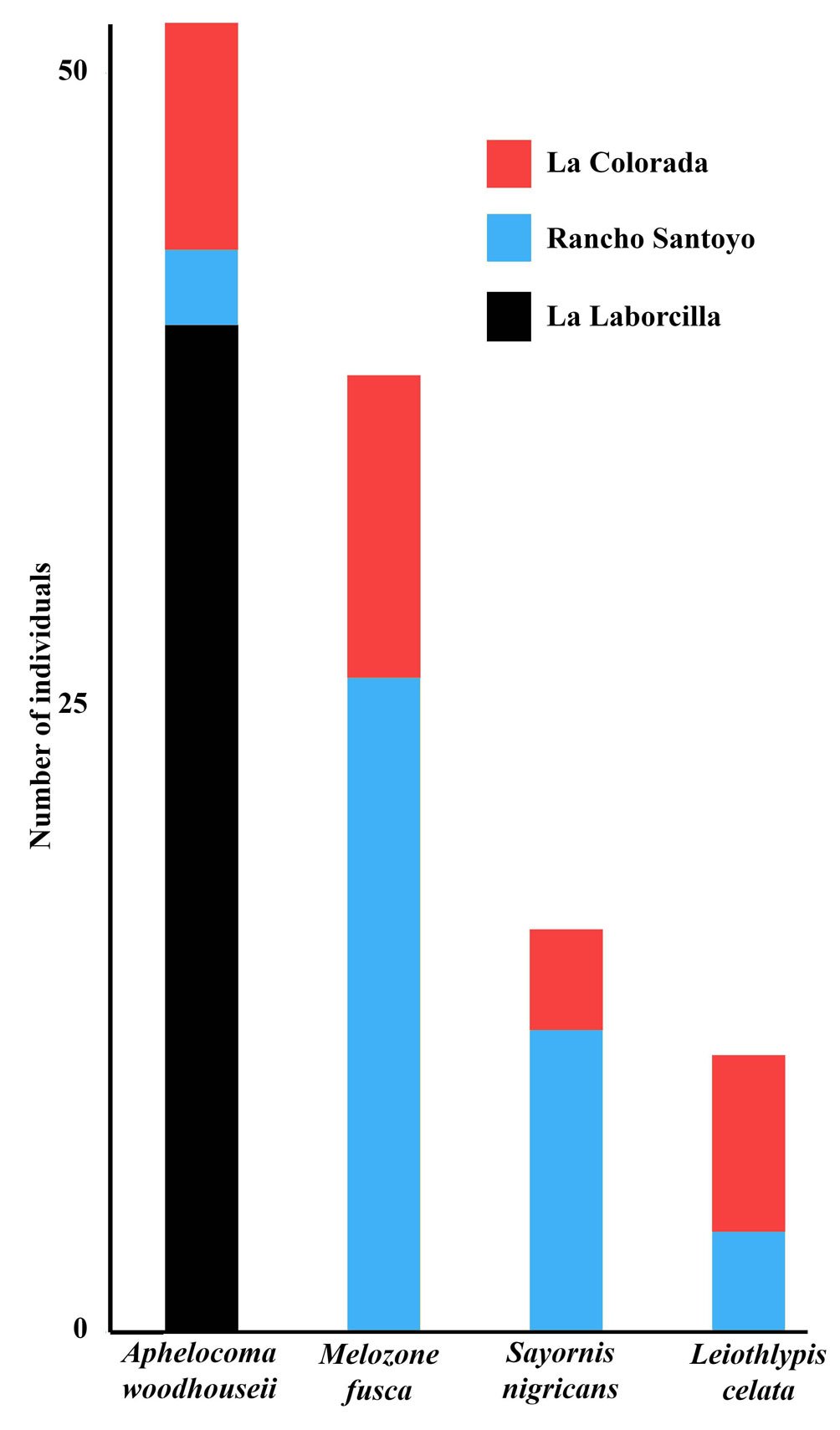
Figure 5. Total abundance of species that had location as part of the best model exploring the influence of locality and survey month, during the 2019-2020 non-breeding season in each of 3 xeroriparian systems in the Llanos de Ojuelos, southern Mexican Altiplano.
La Laborcilla had a total bird count of 213 individuals (162 of 13 resident/breeding species, 48 of 8 migrant species, and 3 of 2 unidentified species), Rancho Santoyo had 353 (197/22, 149/11, and 7/3), and La Colorada, 366 (228/27, 128/16, and 10/3). Most individuals counted were of resident species or of 1 Summer (breeding) resident species (Myiarchus cinerascens),while migrants were a smaller component of the community (Fig. 2). For species richness, the best model did not include locality nor month. The best model explaining overall bird abundance included month (Supplementary material 3), but not locality. Abundance increased from Autumn (September) to Spring (March) with some differences between guilds. Insectivore migrants increased in number into the Winter and then decreased, while granivore migrants began to arrive in December and increased until March (Fig. 2). In all these cases the month of survey was part of the best model, as it was of 11 bird species (Figs. 3, 4; Supplementary material 3). Locality was part of the best model explaining abundance in 4 cases out of 27, all of them individual species (Fig. 5; Supplementary material 3). Aphelocoma woodhouseii and Leiothlypis celata were the only 2 species whose best model included both locality and moth, while the best models for the other species did not include either variable (Supplementary material 3).

Figure 6. Total abundance of birds in different trophic guilds in 3 xeroriparian systems and 3 sections within each, during the 2019-2020 non-breeding season in the Llanos de Ojuelos, southern Mexican Altiplano. Numbers on the circles indicate richness and total abundance, while numbers on the side of the dendrograph indicate similarity between xeroriparian systems, Bird assemblages in Rancho Santoyo and La Colorada were more similar between them than to La Laborcilla (Fig. 6). In PCA graphs, the 3 sections at La Laborcilla grouped closer to each other than those of the other systems. The sections within each system grouped discreetly when binary data was used (Fig. 7 top), but groups overlapped when based on abundance (Fig. 7 bottom). The 3 systems studied differed in the resident/breeding vs. migrant composition of the communities, and sections within systems were also different (Fig. 6). Whereas Rancho Santoyo had a higher proportion of insectivore migrants than the other locations, La Colorada had a higher count of granivore migrants, and La Laborcilla had proportionally more individuals of resident species (Myiarchus cinerascens did not occur in La Laborcilla). In neither case did such patterns occur in the 3 sections of the corresponding system, but only in 2 of Rancho Santoyo’s sections and in 1 and partially in another at La Colorada.

Figure 7. Principal Component arrangement of 3 study sections in each of 3 xeroriparian systems based on their bird composition during the 2019-2020 non-breeding season in the Llanos de Ojuelos, southern Mexican Altiplano. The upper figure is based on binary data (presence/absence of species), and the lower figure, on bird abundance. Ellipses were drawn around the 3 sections of each system by hand. The legends “Up”, “Md”, and “Lw” indicate the upper, middle and lower sections of each system.
The attributes of the plant communities were different between xeroriparian systems (Table 4). La Laborcilla had significantly less ground covered by herbs, whereas Rancho Santoyo and La Colorada were not different in this aspect. La Colorada had significantly denser vegetation from 0 to 75 cm above the ground than the 2 other systems, but visual obstruction at 75-100 cm was not different between the 3 systems. The tallest shrubs and highest trees were significantly taller in Rancho Santoyo than in La Laborcilla, whereas La Colorada was not different from either, and average height both shrubs and trees was significantly greater at Rancho Santoyo than at La Laborcilla, with La Colorada being in between and statistically different from either. Canopy cover was not different between systems. Study sections were all peculiar within the systems, but only in some cases were sections significantly different (Supplementary material 4). Despite slight differences, visual obstruction at the 4 heights assessed was highest in September and October, and then decreased towards their lowest values in March (Fig. 8).
At least 1 habitat attribute was part of the best bird model in all but 3 cases (Tables 5-7), the 3 of them resident species: Zenaida asiatica, Thryomanes bewickii, and Phainopepla nitens. In all cases in which canopy cover was part of the best model, it had a negative effect on bird richness or abundance, while herb density and visual obstruction at 25-75 cm had a negative effect in most of the best models that included them (Tables 5-7). In contrast, visual obstruction at 75-100 cm and mean/maximum height of shrubs/trees had a positive effect.
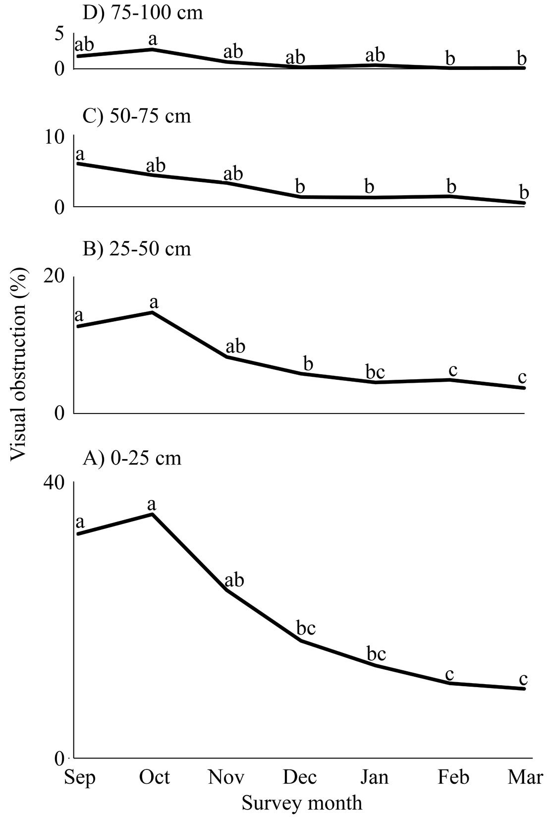
Figure 8. Mean visual obstruction in 4 25-cm vertical layers, between 0 and 100 cm above the ground across 3 sections in each of 3 xeroriparian systems studied during the 2019-2020 non-breeding season in the Llanos de Ojuelos, southern Mexican Altiplano. To reflect the spatial arrangement of the information, the panels are arranged bottom to top. The height stratum to which each graph corresponds is indicated on the graph. Points on each graph with the same letter are not statistically different (p < 0.05).
Discussion
The lack of studies about the role of ephemeral and intermittent xeroriparian systems as key habitats for biodiversity conservation and potential provision of ecological services severely impairs the capability of designing and implementing timely and informed conservation actions. In this study we generated a basic understanding about the composition of bird assemblages in 3 Mexican xeroriparian systems and the habitat attributes that influence them. Our study is particularly pertinent as the results of only 3 other research projects on birds in Mexican xeroriparian systems have been published (Arizmendi et al., 2008; Hinojosa-Huerta et al., 2013; Pérez-Amezola et al., 2020), none of them including ephemeral systems.
The 48 terrestrial species that we recorded represent 20% of all potential terrestrial native birds of the area, excluding swifts (family Apodidae) (based on Howell and Webb [1995]). This is relevant considering that xeroriparian systems, in general, occupy around 5% of the total land surface in western North America (Krueper, 2000), and that those we studied covered approximately 0.1% of the area in which they are located (by delineating them in Google Earth and measuring their area as well as that of the displayed image). According to Partners of Flight (2023) Campylorhynchus brunneicapillus, Spizella atrogularis, Selasphorus rufus/sasin, and Cardellina pusilla have conservation problems, while Accipiter striatus and A. cooperii are protected by Mexican law (Semarnat, 2010). The importance of xeroriparian systems in the region studied is enhanced by the fact that some otherwise woodland bird species largely depend on them, and we have not documented them in any other xeric habitats of the region (Mellink et al., 2016, 2017; Riojas-López & Mellink, 2019; Riojas-López et al., 2019).
Table 4
Vegetation attributes of 3 xeroriparian systems in the Llanos de Ojuelos, southern part of the Mexican Plateau, 2019-2020. Values are estimate ± standard error, except on maximum and minimum heights. Values of any variable with different literal were significantly different (p ≤ 0.05) according to an ANOVA + Tukey post hoc tests. Superscript “ns” indicates that the means were not significantly different.
| Site/section | Herb | Visual obstruction (%) | Hight of shrubs (m) | Height of trees (m) | Canopy | |||||||
| density (1-4) | 0-25 cm | 25-50 cm | 50-75 cm | 75-100 cm | Max | Min | Mean | Max | Min | Mean | cover (%) | |
| La Laborcilla | 1.53 ± 0.38b | 12.00 ± 4.27b | 4.22 ± 2.58b | 0.89 ± 1.06b | 0.40 ± 0.55ns | 2.63 ± 0.32b | 0.23 ± 0.10ns | 0.63 ± 0.01c | 8.37 ± 0.27b | 0.73 ± 0.26ns | 3.58 ± 0.26c | 40.40 ± 8.82ns |
| Rancho Santoyo | 2.52 ± 0.88a | 13.60 ± 16.7b | 3.03 ± 4.75b | 0.85 ± 2.38b | 0.83 ± 2.27ns | 3.55 ± 0.49a | 0.31 ± 0.08ns | 1.41 ± 0.31a | 14.65 ± 3.04a | 1.20 ± 0.44ns | 4.79 ± 0.89a | 39.50 ± 16.83ns |
| La Colorada | 2.70 ± 0.95a | 35.98 ± 17.06a | 16.04 ± 10.83a | 6.40 ± 6.32a | 1.59 ± 2.48ns | 3.14 ±0.76ab | 0.22 ± 0.06ns | 1.21 ± 0.44b | 10.36 ± 3.55ab | 0.87 ± 0.19ns | 4.54 ± 0.54b | 45.48 ±29.86ns |
These species can be considered locally xeroriparian-dependent. They are Accipiter striatus, A. cooperii, Empidonax difficilis occidentalis, Pitangus sulphuratus, Empidonax wrightii, Corthylio calendula, Turdus migratorius, Setophaga coronata, Setophaga townsendi, Piranga ludoviciana, Bubo virginianus, Sphyrapicus varius, and Cardinalis cardinalis. This was also the case of Pipilo maculatus and P. chlorurus, otherwise species of thick shrublands. The system with more xeroriparian-dependent species was La Colorada (9 species) followed by Santoyo (7) and La Laborcilla (6). However, Santoyo had more riparian-dependent individuals (139) than La Colorada (78) and La Laborcilla (45), Setophaga coronata and Corthylio calendula being the most abundant species (Supplementary material 2).
Table 5
Sign of the effects of habitat features on the bird community variables in 3 study sections in each of 3 xeroriparian systems studied during the 2019-2020 non-breeding season in the Llanos de Ojuelos, southern Mexican Altiplano. The only data indicated are that of variables included in the best or more parsimonious model under an information-theoretic approach. Blank cells are of variables not included in such models. Min. indicates minimum, and Max., maximum. Variables with correlation coefficients > 0.85 were merged before the analysis. The intercept is not shown. Actual data is presented in Supplementary material 5.
| Bird community variable | Herb | Visual obstruction (%) | Shrub Min. | Tree Min. | Shrub-tree | Canopy | ||
| Density (1-4) | 0-0.25 cm | 25-75 cm | 75-100 cm | Height (m) | Height (m) | Min./Max. (m) | Cover (%) | |
| Richness | + | – | ||||||
| Abundance | ||||||||
| Overall | – | – | + | – | ||||
| All resident species | – | – | – | |||||
| All migrants | – | + | + | |||||
| Migrant insectivorous birds | – | + | – | |||||
| Migrant granivorous birds | – | + | – |
Table 6
Sign of the effects of habitat features on the abundance of resident species of birds in 3 study sections in each of 3 xeroriparian systems studied during the 2019-2020 non-breeding season in the Llanos de Ojuelos, southern Mexican Altiplano. The only data indicated are that of variables included in the best or more parsimonious model, under an information-theoretic approach. Blank cells are of variables not included in such models. Min. indicates minimum, and Max., maximum. Variables with correlation coefficients > 0.85 were merged before the analysis. The intercept is not shown. Actual data is presented in Supplementary material 5.
| Bird response variable | Herb | Visual obstruction (%) | Shrub Min. | Tree Min. | Shrub-tree | Canopy | ||
| Density (1-4) | 0-0.25 cm | 25-75 cm | 75-100 cm | Height (m) | Height (m) | Min./Max. (m) | Cover (%) | |
| Zenaida asiatica | ||||||||
| Melanerpes aurifrons | – | |||||||
| Sayornis nigricans | + | |||||||
| Aphelocoma woodhouseii | – | – | ||||||
| Psaltriparus minimus | – | + | – | – | ||||
| Phainopepla nitens | ||||||||
| Thryomanes bewickii | ||||||||
| Mimus polyglottos | + | |||||||
| Spinus psaltria | + | + | + | – | ||||
| Spizella passerina | – | – | – | |||||
| Melozone fusca | + | |||||||
| Pipilo maculatus | – | + | – |
Table 7
Sign of the effects of habitat features on the abundance of migratory birds in 3 study sections in each of 3 xeroriparian systems studied during the 2019-2020 non-breeding season in the Llanos de Ojuelos, southern Mexican Altiplano. The only data indicated are that of variables included in the best or more parsimonious model, under an information-theoretic approach. Blank cells are of variables not included in such models. Min. indicates minimum, and Max., maximum. Variables with correlation coefficients > 0.85 were merged before the analysis. The intercept is not shown. Actual data is presented in Supplementary material 5.
| Bird response variable | Herb | Visual obstruction (%) | Shrub Min. | Tree Min. | Shrub-tree | Canopy | ||
| Density (1-4) | 0-0.25 cm | 25-75 cm | 75-100 cm | Height (m) | Height (m) | Min./Max. (m) | Cover (%) | |
| Empidonax wrightii | + | |||||||
| Corthylio calendula | – | + | ||||||
| Troglodytes aedon | + | |||||||
| Turdus migratorius | – | – | + | – | ||||
| Melospiza lincolnii | – | – | + | – | ||||
| Spizella pallida | – | + | – | + | – | |||
| Leiothlypis celata | + | |||||||
| Setophaga coronata | – | |||||||
| Cardellina pusilla | + |
Resident species increased their abundance from December through March (Figs. 2, 3), a pattern that could have been driven by 3 processes, not necessarily mutually exclusive: 1) resident species that might breed in xeroriparian habitats disperse to feed in other habitats in the region after nesting, might have begun to congregate for the upcoming breeding season, which would make the different habitats complementary (Dunning et al., 1992); 2) species like the P. maculatus might become more detectable as breeding-associated territoriality and courting behaviors develop; 3) migrating individuals of northern populations of species that locally remain resident might pass through the region in the Spring (perhaps S. passerina; Fig. 4).
The increase in abundance of the resident species as the season progressed was combined with the addition of migratory species in their northbound Winter-Spring migration. The pattern observed in our study is similar to that in the lower Colorado River in southwestern Arizona, where more birds migrate during the Spring than during the Autumn and suggests that some species migrate via different routes and/or use different habitats during the latter (Carlisle et al., 2009). According to our data, the region is part of the Spring migration route, but not, or less so, of the Autumn route.
Birds assemble differently in response to habitat characteristics (Wiens & Rotenberry, 1981), although bird-habitat relationships are complex (Strong & Bock, 1990). In our study, habitat characteristics were part of the best model in 78% of the cases (Tables 5-7). Three habitat variables more consistently affected bird assemblages and species. The first was that the averaged minimum and maximum height of shrubs and trees influenced birds positively, which conforms with general known principles in bird ecology (Brand et al., 2008; MacArthur & MacArthur, 1961; Merrit & Bateman, 2012; Rockwell & Stephen, 2018), and with findings in other xeroriparian systems (Brand et al., 2008). The second was that closed canopies had a negative effect. Closed canopies have been found to influence birds negatively by reducing light at ground level resulting in a less developed herb and shrub community (Beedy, 1981). The third case was that herb vertical density at 25-75 cm had also a negative effect. But this is a spurious outcome that resulted from the dense herb layer at the beginning of the study (Fig. 8), when bird abundance variables were lower, while the circannual process of herbs drying and decaying in the late Autumn and early Winter causes low herb cover coinciding with the increase in bird abundance (Figs. 2, 3).
The bird assemblages of the xeroriparian systems studied not only were different from each other, but also varied internally, between sections (Figs. 6, 7). The arrangement of the 9 sections according to their species presence/absence in axis 1, explaining 33% of the variance, follows a clear gradient (Fig. 7 top). On the left side are sections with steep, narrow, and rocky ravines with large boulders, dominated by oaks and junipers that form a close canopy with little understory herbaceous vegetation. On the right, wide and open pebbled washes, dominated by a more heterogeneous tree community composed of peppertrees, arborescent nopales, and huisaches, with a well-developed herbaceous layer. The bird communities responded to this gradient with increasing richness and abundance from left to right.
In the same graph, axis 2 follows a gradient from a well-developed shrub community and abundant litter and wetter soil to no or scarce shrubs with a dense herbaceous layer and drier ground. This gradient apparently drives the food resources available to birds, as suggested by the preponderant bird guilds in the different sections (Fig. 6): insects in its lower end to seeds in the upper end. Overall, La Colorada with the most heterogeneous sections, vegetation-wise, had also the richest bird assemblage, while La Laborcilla, with the most homogenous sections, had the poorest one, with Rancho Santoyo intermediate in both attributes (Table 4; Fig. 6; Supplementary material 5). Using bird abundance instead of binary information rearranged the PCA graph layout (Fig. 7 lower) because of the effect of species that were widespread and abundant, but without losing a resemblance to the species presence/absence PCA.
Vertical structure is important for birds, but floristic composition can also influence their diversity (Fleishman et al., 2003; Rotenberry, 1985). For example, oaks are of little attraction to most birds (Powell & Steidl, 2015), and their dominance at La Laborcilla and the upper section of La Colorada coincided with the lower richness and abundance of their bird assemblages (Fig. 6; Supplementary material 2). Rancho Santoyo supported more xeroriparian-dependent individuals, mostly of Setophaga coronata and Corthylio calendula, both small insectivorous birds. The middle and upper sections where these 2 species thrived had large cottonwoods (Populus fremontii) and willows (Salix bonplandiana). In contrast, in the middle section of La Colorada, which also had tall trees but were peppertrees and arborescent nopales, these 2 bird species were much less abundant.
Each of the systems studied had a distinct signature given by one species or dominant bird guild(s), although such signature was largely due to the assemblages in the individual sections (Fig. 6). The signature species at Laborcilla was Aphelocoma woodhouseii, whose primary habitat includes oak and juniper forests, where it typically feeds on juniper berries in the Autumn and Winter (Fig. 5; Cornell Lab of Ornithology, 2019). Although the upper Colorada section grouped with La Laborcilla, with which it shared oaks, lacked junipers and was not used by Aphelocoma woodhouseii. Their close PCA grouping rather resulted from their shared poor bird assemblages. Rancho Santoyo can be identified with migrant insectivorous birds and La Colorada with migrant granivorous birds, in concordance with the explanation on the PCA arrangement provided above.
The lower proportion and abundance of migratory insectivorous birds and absence of granivorous birds at La Laborcilla might have been caused by its less developed understory vegetation and enclosed canyon conditions. In contrast, Rancho Santoyo´s upper and middle section provided the best habitat for insectivore migrants. This system was exuberant in herb and shrub foliage, likely as a result of the longer presence of ground humidity, but had also plenty of sunny spots; and the system bordered open rangeland, providing lengthy, sharp borders, especially in its upper and middle sections. Granivore migrants were a small component of the communities we documented, and they were present almost exclusively in La Colorada´s middle section. This site had an open canopy and combined taller shrubs with denser and taller herbs than in the other sections of the same and the 2 other systems, providing higher habitat heterogeneity and, likely, more seeds. A more developed herb-shrub stratum at 0-75 cm at La Colorada than at other sites provided good escape cover adjacent to open patches that provided seeds (Table 4; Supplementary material 4).
As our data exhibit, habitats associated with non-perennial xeroriparian streams are far from uniform, not only between systems but also within them. At a landscape level they are clearly keystone structures, at least for the birds but surely for other groups as well, both collectively and individually. The 3 systems studied by us cover about 55 ha, roughly 0.1% of the area in which they occur. However, they supported 20% of the potential species of terrestrial birds of the region, including 15 that we have recorded only in such riparian habitat. Our data exhibit that in addition to their importance for resident species, some ephemeral and intermittent xeroriparian habitat in the southern part of the Mexican Altiplano are important for northbound Spring migrating birds.
Our study is a first approximation to the ecological role of xeroriparian systems in the region. However, many issues, like their importance as nesting habitat, provision of food, climatic protection, interaction with adjacent and farther away habitats, among others, remain to be studied. Nevertheless, if these xeroriparian habitats disappear, regional biodiversity would be impacted. Not only 1 or a few, but many or all xeroriparian systems, and their different sections in the region studied by us should be targeted for conservation management. Xeroriparian systems have long been considered important elements of the landscape and their conservation needs recognized. However, such consideration, and the actions derived from it, usually focus on perennial streams with their lush arboreal communities. This focus is biased and excludes an important part of xeroriparian habitat: that created by ephemeral and intermittent streams. Despite their low consideration in research and in conservation agendas, as our study and a few others have demonstrated, ephemeral and intermittent xeroriparian habitat can play a crucial role in arid and semiarid lands (Johnson & Haight, 1985; Levick et al., 2008; Sánchez-Montoya et al., 2017; Szaro & Jakle, 1985). Despite covering less than 0.1% of the region´s area, in our study they supported 20% of all terrestrial species that we documented in the region (Mellink et al., 2016, 2017; Riojas-López & Mellink, 2019; Riojas-López et al., 2019), while those that we documented only in xeroriparian systems account for 9% of all species documented. A scenario of ecological importance of non-perennial xeroriparian systems and research and management neglect are likely to occur in many other arid and semiarid regions of the world. Hence, it might be time to join forces and impulse a global agenda for their conservation, which is now especially pertinent in view of the ongoing climate change in which drier and hotter regimes are predicted.
Acknowledgements
Jaime Luévano Esparza, David H. Almanzor, Santiago Cortés, and Marco A. Carrasco assisted during field work. Access and research permission were granted kindly by owners Family Santoyo (Rancho Santoyo) and Enrique Campos (La Laborcilla), and ranch manager Melquíades Contreras (La Colorada). Ezequiel Martínez and Margarita Chávez provided logistic support. Two anonymous reviewers provided extensive and valuable comments. Our greatest appreciation to all of them. Financial support was provided by the Centro de Investigación Científica y de Educación Superior de Ensenada (CICESE), the Universidad de Guadalajara, and the first two authors´ personal funds. The Consejo Nacional de Humanidades, Ciencias y Tecnologías supported MM-O through a M.Sc. scholarship.
References
Arizmendi, M. D., Dávila, P., Estrada, A., Figueroa, E., Márquez-Valdelamar, L., Lira, R. et al. (2008). Riparian mesquite bushes are important for bird conservation in tropical arid Mexico. Journal of Arid Environments, 72,1146–1163. https://doi.org/10.1016/j.jaridenv.2007.12.017
Beedy, E. C. (1981). Bird communities and forest structure in the Sierra Nevada of California. Condor, 83,97–105. https://doi.org/10.2307/1367415
Brand, L. A., White, G. C., & Noon, B. R. (2008). Factors influencing species richness and community composition of breeding birds in a desert riparian corridor. Condor, 110,199–210. https://doi.org/10.1525/cond.2008.8421
Burnham, K. P., & Anderson, D. R. (2002). Model selection and multimodel inference: A practical information-theoretic approach. 2nd Ed. New York: Springer-Verlag.
Carlisle, J. D., Skagen, S. K., Kus, B. E., Van Riper III, C., Paxtons, K. L., & Kelly, J. F. (2009). Landbird migration in the American West: recent progress and future research directions. Condor, 111,211–225. https://doi.org/10.1525/cond.2009.080096
Challenger, A. (1998). Utilización y conservación de los ecosistemas terrestres de México. México D.F.: Comisión Nacional para el Conocimiento y Uso de la Biodiversidad, Instituto de Biología (UNAM), and Agrupación Sierra Madre.
Chesser, R. T., Billerman, S. M., Burns, K. J., Cicero, C., J. L. Dunn, J. L., Hernández-Baños, B. E. et al. (2023). Check-list of North American Birds (online). American Ornithological Society. Retrieved on March 14th, 2024 from: https://checklist.americanornithology.org/taxa/
Conabio (Comisión Nacional para el Conocimiento y Uso de la Biodiversidad). (1998). La diversidad biológica de México: estudio de país. México D.F.: Comisión Nacional para el Conocimiento y Uso de la Biodiversidad.
Conabio (Comisión Nacional para el Conocimiento y Uso de la Biodiversidad). (2008). Capital natural de México, vol. I: Conocimiento actual de la biodiversidad. México D.F.: Comisión Nacional para el Conocimiento y Uso de la Biodiversidad.
Cornell Lab of Ornithology (2019). Woodhouse´s Scrub-Jay. Retrieved on June 7th, 2023 from: https://www.allaboutbirds.org/guide/Woodhouses_Scrub-Jay/lifehistory#
Datry, T., Bonada, N., & Boulton, A. J. (2017). Conclusions: recent advances and future prospects in the ecology and management of intermittent rivers and ephemeral streams. In T. Datry, N. Bonada, & A. J. Boulton (Eds.), Intermittent rivers and ephemeral streams: ecology and management (pp. 563–584). San Diego, CA: Academic Press.
Dunning, J. B., Danielson, B. J., & Pulliam, H. R. (1992). Ecological processes that affect populations in complex landscapes. Oikos, 65,169–175. https://doi.org/10.2307/3544901
Fleishman, E., McDonal, N., Nally, R. M., Murphy, D. D., Walters, J., & Floyd, T. (2003). Effects of floristics, physiognomy and non-native vegetation on riparian bird communities in a Mojave Desert watershed. Journal of Animal Ecology, 72, 484–490. https://doi.org/10.1046/j.1365-2656.2003.00718.x
Harker, M., García R., L. A., & Riojas-López, M. E. (2008). Composición florística de cuatro hábitats en el rancho Las Papas de Arriba, municipio de Ojuelos de Jalisco, Jalisco, México. Acta Botanica Mexicana, 85,1–29.
Hays, R. L., Summers, C., & Seitz, W. L. (1981). Estimating wildlife habitat variables. Washington DC: U.S. Fish and Wildlife Service.
Hinojosa-Huerta, O., Soto-Montoya, E., Gómez-Sapiens, M., Calvo-Fonseca, A., Guzmán-Olachea, R., Butrón-Méndez, J. et al. (2013). The birds of the Ciénega de Santa Clara, a wetland of international importance within the Colorado River delta. Ecological Engineering, 59,61–73. https://doi.org/10.1016/j.ecoleng.2013.03.005
Johnson, R. R., & Haight, L. T. (1985). Avian use of xeroriparian ecosystems in the North American warm deserts. In R. R. Johnson, C. D. Ziebell, D. R. Patton, P. F. Ffolliott, P. F., & R. H. Hamre (Tech. Coords.), Riparian ecosystems and their management: reconciling conflicting uses (pp. 156–160). General Technical Report RM-GTR-120. Fort Collins, CO: U.S. Department of Agriculture, Forest Service, Rocky Mountain Forest and Range Experiment Station.
Kirkpatrick, C., Conway, C., & LaRoche, D. (2009). Surface water depletion and riparian birds. Tucson, Arizona: Arizona Cooperative Fish and Wildlife Research Unit.
Knopf, F. L. (1985). Significance of riparian vegetation to breeding birds across an altitudinal cline. In R. R. Johnson, C. D. Ziebell, D. R. Patton, P. F. Ffolliott, & R. H. Hamre (Tech. Coords.), Riparian ecosystems and their management: reconciling conflicting uses (pp. 105–111). General Technical Report RM-GTR-120. Fort Collins, CO: U.S. Department of Agriculture, Forest Service, Rocky Mountain Forest and Range Experiment Station.
Knopf, F. L., Johnson, R. R., Rich, T., Samson, F. B., & Szaro, R. C., 1988. Conservation of riparian ecosystems in the United States. Wilson Bulletin, 100,272–284. http://www.jstor.org/stable/4162566
Krueper, D. J. (1993). Effects of land use practices on western riparian ecosystems. In D. M. Finch, & P. W. Stangel (Eds.), Status and management of neotropical migratory birds (pp. 321–330). General Technical Report RM-229. Fort Collins, CO: U.S. Department of Agriculture, Forest Service, Rocky Mountain Forest and Range Experiment Station.
Krueper, D. J. (1996). Effects of livestock management on southwestern riparian ecosystems. In D. W. Shaw, & D. M. Finch (Tec. Coords.), Desired future conditions for Southwestern riparian ecosystems: bringing interests and concerns together (pp. 281–301). General Technical Report RM-GTR-272. Fort Collins, CO: U.S. Department of Agriculture, Forest Service, Rocky Mountain Forest and Range Experiment Station.
Krueper, D. J. (2000). Conservation priorities in naturally fragmented and human-altered riparian habitats of the arid West. In R. Bonney, D. N. Pachley, R. J. Cooper, & L. Nioes (Eds.), Strategies for bird conservation: the partners in flight planning process (pp. 88–90). USDA Forest Service Proceedings RMRS-P-16. Ogden, Utah, U.S.A.: Rocky Mountain Research Station.
Levick, L., Fonseca, J, Goodrich, D., Hernández, M., Semmens, D., Stromberg, J. et al. (2008). The ecological and hydrological significance of ephemeral and intermittent streams in the arid and semi-arid American southwest. Washington D.C.: Office of Research and Development, U.S. Environmental Protection Agency.
MacArthur R. H., & MacArthur, J. W. (1961). On bird species diversity. Ecology, 423,594–598. https://doi.org/10.2307/1932254
McDonough, O. T., Hosen, J. D., & Palmer, M. A. (2011). Temporary streams: the hydrology, geography, and ecology of non-perennially flowing waters. In H. S. Elliot, & L. E. Martin (Eds.), River ecosystems: dynamics, management and conservation (pp. 259–289). Hauppauge, N.Y.: Nova Science.
Mellink, E., & Riojas-López, M. E. (2020). Livestock and grassland interrelationship along five centuries of ranching the semiarid grasslands on the southern highlands of the Mexican Altiplano. Elementa Science of the Anthropocene, 8, 20. https://doi.org/10.1525/elementa.416
Mellink, E., Riojas-López, M. E., & Giraudoux, P. (2016). A neglected opportunity for bird conservation: the value of a perennial, semiarid agroecosystem in the Llanos de Ojuelos, central Mexico. Journal of Arid Environments, 124,1–9. https://doi.org/10.1016/j.jaridenv.2015.07.005
Mellink E., Riojas-López, M. E., & Cárdenas-García, M. (2017). Biodiversity conservation in an anthropized landscape: Trees, not patch size drive bird community composition in a low-input agroecosystem. Plos One, 12, e0179438. https://doi.org/10.1371/journal.pone.0179438
Merritt, D. M., & Bateman, H. L. (2012). Linking stream flow and groundwater to avian habitat in a desert riparian system. Ecological Applications, 22, 1973–1988. https://doi.org/10.1890/12-0303.1
Neate-Clegg, M. H. C., Horns, J. J., Buchert, M., Pope, T. L., Norvell, R., Parrish, J. R. et al. (2021). The effects of climate change and fluctuations on the riparian bird communities of the arid Intermountain West. Animal Conservation, 25,325–341. https://doi.org/10.1111/acv.12755
Nieto-Samaniego, Á. F., Alaniz-Ávarez, S. A., & Camprubí, A. (2005). La Mesa Central de México: estratigrafía, estructura y evolución tectónica cenozoica. Boletín de la Sociedad Geológica Mexicana, 57, 285–318. https://doi.org/10.18268/bsgm2005v57n3a3
Partners in Flight Databases. (2023). Retrieved on July 13th,
2023 from: https://pif.birdconservancy.org/avian-conserva
tion-assessment-database-scores/
Patten, D. T., Carothers, S. W., Johnson, R. R., & Hamre, R. H. (2018). Development of the science of riparian ecology in the semi-arid western United States. In R. R. Johnson, S. W. Carothers, D. M. Finch, K. J. Kingsley, & J. T. Stanley (Tech. Eds.), Riparian research and management: past, present, future, Volume 1 (pp. 1–16). General Technical Report RM-GTR-373. Fort Collins, CO: U.S. Department of Agriculture, Forest Service, Rocky Mountain Forest and Range Experiment Station.
Pérez-Amezola, M. C., Gatica-Colima, A. B. M. Cuevas-Ortalejo, D. M., Martínez-Calderas, J. M., & Vital-García, C. (2020). Riparian biota of the Protected Area of Flora and Fauna Santa Elena canyon, Mexico. Revista Bio Ciencias, 7, e798. https://doi.org/10.15741/revbio.07.e798
Powell, B. F., & Steidl, R. J. (2015). Influence of vegetation on montane riparian bird communities in the sky islands of Arizona, USA. Southwestern Naturalist 60,65–71. https://doi.org/10.1894/MCG-09.1
Riojas-López, M. E., & Mellink, E. (2019). Registros relevantes de aves en el sur del Altiplano Mexicano. Huitzil, 20, e-513. https://doi.org/10.28947/hrmo.2019.20.2.457
Riojas-López, M. E., Mellink, E., & Almanzor-Rojas, D.H. (2019). Estado del conocimiento de los carnívoros nativos (Mammalia) en un paisaje antropizado del Altiplano Mexi-
cano: el caso de Los Llanos de Ojuelos. Revista Mexicana de Biodiversidad, 90,e902669. https://doi.org/10.22201/ib.
20078706e.2019.90.2669
Riparian Habitat Joint Venture (2004). The riparian bird conser-
vation plan: a strategy for reversing the decline of riparian associated birds in California. Ver. 2.0. Retrieved on September
28th, 2021 from: https://web.archive.org/web/2018072200
1457id_/http://www.prbo.org/calpif/pdfs/riparian_v-2.pdf
Rockwell, S. M., & Stephens, J. L. (2018). Habitat selection of riparian birds at restoration sites along the Trinity River, California. Restoration Ecology, 26,767–777. https://doi.org/10.1111/rec.12624
Rosenberg, K. V, Dokter, A. M., Blancher, P. J., Sauer, J. R., Smith, A. C., Smith, P. A. et al. (2019). Decline of the North American avifauna. Science, 366,120–124. https://doi.org/10.1126/science.aaw1313
Rosgen, D. A. (1994). A classification of natural rivers. Catena, 22,169–199. https://doi.org/10.1016/0341-8162(94)90001-9
Rotenberry, J. T. (1985). The role of habitat in avian community composition: physiognomy or floristics? Oecologia, 67,213– 217. https://doi.org/10.1007/BF00384286
Sánchez-Montoya, M. M., Moleón, M., Sánchez-Zapata, J.A., & Escoriza, D. (2017). The biota of intermittent and ephemeral rivers: amphibians, reptiles, birds, and mammals. In T. Datry, N. Bonada, & A. J. Boulton (Eds.), Intermittent rivers and ephemeral streams: ecology and management (pp. 299–322). San Diego, CA: Academic Press.
Şekercioǧlu, C. H., Loarie, S. R., Oviedo-Brenes, F., Mendenhall, C. D., Daily, G. C., & Ehrlich, P. R. (2015). Tropical countryside riparian corridors provide critical habitat and connectivity for seed-dispersing forest birds in a fragmented landscape. Journal of Ornithology, 156,343–353. https://doi.org/10.1007/s10336-015-1299-x
Semarnat (Secretaría del Medio Ambiente y Recursos Naturales). (2010). Norma Oficial Mexicana NOM-059-SEMARNAT-2010, Protección ambiental – Especies nativas de México de flora y fauna silvestres – Categorías de riesgo y especificaciones para su inclusión, exclusión o cambio – Lista de especies en riesgo. Diario Oficial de la Federación. 30 de diciembre de 2010, Segunda Sección, México.
Seymour, C. L., & Simmons, R. E. (2008). Can severely fragmented patches of riparian vegetation still be important for arid-land bird diversity? Journal of Arid Environments, 72,2275–2281. https://doi.org/10.1016/j.jaridenv.2008.07.014
Skagen, S. K., Melcher, C. P., Howe, W. H., & Knopf, F. L. (1998). Comparative use of riparian corridors and oases by migrating birds in southeast Arizona. Conservation Biology, 12,896–909. https://doi.org/10.1111/j.1523-1739.1998.96384.x
Strong, T. R., & Bock, C. E. (1990). Bird species distribution patterns in riparian habitats in southeastern Arizona. Condor, 92,866–885. https://doi.org/10.2307/1368723
Szaro, R. C., & Jakle, M. D. (1985). Avian use of a desert riparian island and its adjacent scrub habitat. Condor, 87,511–519. https://doi.org/10.2307/1367948
Wiens, J. A., & Rotenberry, J. T. (1981). Habitat associations and community structure of birds in shrubsteppe environments. Ecological Monographs, 51,21–41. https://doi.org/10.2307/
2937305

Perfil de leucocitos como biomarcador hematológicoen poblaciones de la salamandra de arroyo Ambystoma ordinarium
Carolina González-Pardo a, Ireri Suazo-Ortuño a, *, Cinthya Mendoza-Almeralla b, David Tafolla-Venegas c, Yurixhi Maldonado-López a y Esperanza Meléndez-Herrera a
a Universidad Michoacana de San Nicolás de Hidalgo, Instituto de Investigaciones sobre los Recursos Naturales, Avenida San Juanito Itzícuaro s/n, Nueva Esperanza, 58330 Morelia, Michoacán, México
b Universidad Autonóma del Estado de Hidalgo, Instituto de Ciencias Básicas e Ingeniería, Centro de Investigaciones Biológicas, Laboratorio de Ecología de Poblaciones, Km 4.5 carretera Pachuca-Tulancingo, 42184 Mineral de La Reforma, Hidalgo, México
c Universidad Michoacana de San Nicolás de Hidalgo, Facultad de Biología, Edificio R, Ciudad Universitaria, 58030 Morelia, Michoacán, México
*Autor de correspondencia: ireri.suazo@umich.mx (I. Suazo-Ortuño)
Recibido: 7 agosto 2023; aceptado: 22 febrero 2024
Resumen
La evaluación del perfil de leucocitos como biomarcador hematológico en las poblaciones de anfibios es cada vez más común en estudios ecológicos en especies amenazadas o en declive. En este estudio evaluamos y comparamos el perfil de leucocitos y el índice neutrófilos/linfocitos (N/L) en frotis de sangre periférica de Ambystoma ordinarium en 3 tipos de hábitats: conservados, urbanizados y agrícolas. Consideramos al perfil leucocitario como un endpoint inmunológico, ya que nos puede proporcionar información sobre la respuesta inmunológica del organismo. De acuerdo con los resultados encontrados, en los individuos de A. ordinarium de los sitios urbanizados y agrícolas se detectaron aumentos en las proporciones de eosinófilos, basófilos y monocitos, y una disminución en las proporciones de linfocitos. Asimismo, en los individuos de los sitios urbanizados y agrícolas se detectaron aumentos en el número de neutrófilos banda, además se reporta por primera vez el hallazgo de células plasmáticas en la sangre de esta especie. En general, los perfiles de leucocitos de los individuos de A. ordinarium en los sitios urbanizados y agrícolas observados en este estudio, podrían interpretarse como respuestas fisiológicas a la perturbación ambiental.
Palabras clave: Hábitats perturbados; Respuesta inmunitaria; Índice N/L; Neutrófilos banda; Células plasmáticas; Achoque michoacano
© 2024 Universidad Nacional Autónoma de México, Instituto de Biología. Este es un artículo Open Access bajo la licencia CC BY-NC-ND
(http://creativecommons.org/licenses/by-nc-nd/4.0/).
Leukocyte profile as hematologic biomarker in populations of the mountain salamander, Ambystoma ordinarium
Abstract
Assessing the leukocyte profile as a hematological biomarker is now frequently used in ecological studies of threatened or declining species. In this study, we evaluated and compared leukocytes profile and neutrophils/lymphocytes (N/L) ratio in peripheral blood smears of the salamander Ambystoma ordinarium in 3 types of habitats: urbanized, agricultural, and conserved. We considered leukocyte profiles as an immunological endpoint, since it can provide information about the immunological response. Results indicated that A. ordinarium individuals from the urbanized and agricultural sites presented higher proportions of neutrophils, eosinophils, basophils and monocytes and a decrease in the proportions of lymphocytes. Agricultural habitats presented higher N/L ratios. Likewise, in the individuals of urbanized and agricultural sites an increase was registered in the number of neutrophils with a band nucleus, in addition, the finding of plasma cells in the blood of this species is reported for the first time. In general, leukocyte profiles of A. ordinarium individuals in urbanized and agricultural sites observed in this study suggest that these profiles can be interpreted as physiological responses to environmental disturbance.
Keywords: Disturbed habitats; Immune response; N/L ratio; Band neutrophils; Plasma cells; Achoque michoacano
Introducción
En la actualidad, una de las preocupaciones más importantes en la conservación de vida silvestre es la pérdida y disminución global de las especies de anfibios (Alvarado, 2021). Los cambios en los hábitats asociados a las actividades antropogénicas y las enfermedades infecciosas representan las principales amenazas (Wake y Vredenburg, 2008). Sin embargo, científicos en todo el mundo, consideran que no existe una sola causa potencial, sino que éstos y otros factores pueden actuar mediante sinergias contribuyendo en la disminución de sus poblaciones (Lips et al., 2005; Stuart et al., 2004).
Los anfibios, pueden ser más vulnerables a los cambios en sus hábitats en comparación con el resto de los vertebrados, por 2 razones principales: poseen una piel delgada y porosa que es permeable al agua, y son organismos ectotermos, por lo que dependen de su entorno para conservar su temperatura (Duellman y Trueb, 1994). Por estos motivos, la evaluación del estado de salud de las poblaciones de anfibios es cada vez más común en estudios ecológicos en especies amenazadas o en declive (Barriga-Vallejo et al., 2015; Das y Mahapatra, 2014; Shutler y Marcogliese, 2011). Los perfiles de leucocitos han sido evaluados con mayor frecuencia porque proporcionan información sobre el estado inmunológico y permiten detectar cambios fisiológicos y patológicos tempranos en los individuos, sobretodo, estudios recientes han comenzado a incorporarlos como biomarcadores para evaluar la salud de los individuos y de su ambiente (Barni et al., 2007; Cabagna et al., 2005; Davis et al., 2010; Salinas et al., 2015, 2019).
Los leucocitos (linfocitos, neutrófilos, eosinófilos, basófilos y monocitos) son células sanguíneas que forman parte del sistema inmunitario, desempeñando funciones cruciales en la defensa contra infecciones y enfermedades (Thrall, 2004). De esta forma, los leucocitos en sangre pueden aumentar rápidamente en una infección, por ejemplo, aumentos en las proporciones de eosinófilos se han asociado con infecciones parasitarias (Davis y Golladay, 2019; Ramírez-Hernández et al., 2019) y en evidencia reciente, se han reportado aumentos en las frecuencias de linfocitos maduros e inmaduros (Salinas et al., 2019). El perfil de leucocitos también ha sido evaluado con éxito como indicador de estrés en poblaciones en ambientes perturbados y alteraciones morfológicas como el aumento de neutrófilos sin segmentación nuclear se han relacionado con ambientes contaminados con desechos urbanos y agrícolas (Barni et al., 2007; Cabagna et al., 2005; Ramírez-Hernández et al., 2019; Romanova y Romanova, 2003).
En México, habitan 14 especies del género Ambystoma (Ramírez-Bautista et al., 2023) y se ha estudiado el perfil de leucocitos en algunas especies como biomarcador de inflamación y estrés asociado a perturbaciones antropogénicas (Barriga-Vallejo et al., 2015; Ramírez-Hernández et al., 2019). La salamandra de arroyo Ambystoma ordinarium se distribuye en el noreste de Michoacán y se encuentra catalogada como en peligro de extinción por la IUCN (2024), y como especie protegida por el gobierno de México (Semarnat, 2010). Particularmente, en varios sitios del área de distribución de esta especie existe un fuerte impacto sobre los arroyos que habita debido a presiones de urbanización, actividades agrícolas y ganaderas (Soto-Rojas, 2012). Considerando el contexto en el que se encuentra esta especie, es importante monitorear sus poblaciones, sobre todo las que están sujetas a la continua perturbación de sus hábitats. Por lo tanto, el objetivo de este estudio fue evaluar y comparar los perfiles de leucocitos como biomarcador hematológico en poblaciones de A. ordinarium de hábitats con diferentes grados de perturbación: conservados, urbanizados y agrícolas.
Materiales y métodos
Se realizaron 2 visitas, la primera en noviembre de 2020 y la segunda en marzo de 2021 a 9 sitios con arroyos habitados por A. ordinarium condiferentes grados de perturbación en Michoacán (fig. 1).Los sitios 1, 2 y 3 se encuentran en zonas conservadas en los municipios de Charo, Morelia y Zinápecuaro. En estos sitios, la vegetación está representada por bosque de pino y pino-encino y no se encuentran afectados por la urbanización, cultivos ni zonas de pastoreo.
Los sitios 4, 5 y 6 son urbanizados y se localizan en la Ciudad de Morelia, la cual tiene una extensión de 1,333 km2 y presenta más de 500,000 habitantes (Magaña-Martínez y Reyes Camacho, 2012; tabla 1, fig. 1). Cada sitio se encuentra a una distancia mínima de 3 km uno con respecto a otro, por lo que corresponden a 3 poblaciones independientes de acuerdo a la poca vagilidad de la especie reportada por Montes-Calderón et al. (2011). Se consideraron los sitios como perturbados debido a: 1) la presencia de construcciones urbanas (López- Granados et al., 2008; Magaña-Martínez y Reyes Camacho, 2012), 2) el vertimiento de aguas contaminadas con fertilizantes y pesticidas (López- Granados et al., 2008) y 3) se encuentran a menos de 1 km de avenidas principales de la ciudad de Morelia (Téllez-Ramírez, 2012).
Los sitios 7, 8 y 9 se encuentran en zonas agrícolas en los municipios de Queréndaro, Indaparapeo y Zinapécuaro (fig. 1). Estos sitios presentan arroyos permanentes con escasa vegetación ribereña y se consideran perturbados porque durante el muestreo de este estudio, estaban rodeados de cultivos de maíz y potreros, y no presentaban vegetación de bosque de pino y pino-encino.
En cada arroyo se realizó una búsqueda intensiva de los ejemplares mediante la técnica de inspección por encuentro visual (VES) (Crump y Scott, 1994). Una vez localizados, se capturaron con red de mano y se colocaron en recipientes con agua de su medio para evitar su desecación. Inmediatamente, en el sitio de colecta, se manipuló a cada ejemplar con guantes estériles y se obtuvo una gota de sangre periférica de un pequeño corte de una de las branquias, llevando a cabo el procedimiento sin sacrificar a los individuos. La gota de sangre se colocó en el extremo de un portaobjetos limpio y con ayuda de un segundo, el cual se colocó en un ángulo de 45° por delante de la gota, se lo hizo retroceder hasta tocar la gota, luego se deslizó ejerciendo una presión suave y firme hacia delante. Cada frotis sanguíneo se secó a temperatura ambiente por 3 min y se fijó con metanol. Al final del procedimiento todos los organismos se liberaron en sus respectivos arroyos de origen. El manejo de las salamandras y las muestras se realizó con el permiso de colecta científica número SGPA/DGVS/13339/19 otorgado por la Semarnat.
Los frotis sanguíneos fueron llevados al laboratorio de Parasitología de la Universidad Michoacana de San Nicolás de Hidalgo (UMSNH) y se cubrieron con el colorante no diluido de Wright, dejándose reposar durante 5 min. Posteriormente, se les agregó solución buffer de Wright gota a gota, hasta que apareció una película metálica sobre la muestra, después se dejaron reposar por 5 min. Finalmente, los frotis fueron lavados con agua destilada, hasta que el colorante se lavó y se dejaron secar.

Figura 1. Mapa de la ubicación de los sitios de estudio de A. ordinarium en algunos municipios de Michoacán. 1. 5.7 km al este de Jaripeo, 2. Agua Zarca, 3. 8.9 km al oeste de Bocaneo, 4. Puente campestre, 5. Filtros viejos, 6. Río Chiquito, 7. 14 km al sur de Queréndaro, 8. 0.75 km al sur de Ziróndaro, 9. 10.86 km al sureste del Municipio de Queréndaro.
Tabla 1
Datos de colecta de Ambystoma ordinarium. Se muestra el nombre, las coordenadas y la categoría de los sitios de colecta y el número y talla de los organismos colectados.
| Número y nombre de sitio | Coordenadas | Categoría del sitio | Individuos colectados en invierno 2020 | Individuos colectados en primavera 2021 | Longitud LHC en mm |
| 1. 5.7 km al este de Jaripeo | 19°40’28.3” N, 101°01’44.9” O | Conservado | 4 | 3 | 74 a 77 |
| 2. Agua Zarca | 19°34’28.9” N, 101°07’28.2” O | Conservado | 3 | 13 | 66 a 77 |
| 3. 8.9 km al oeste de Bocaneo | 19°50’28.6” N, 100°43’55.1” O | Conservado | 0 | 13 | 67 a 88 |
| 4. Puente campestre | 19°40’31.3” N, 101°09’27.5′′ O | Urbanizado | 3 | 3 | 79 a 98 |
| 5. Filtros Viejos | 19°40’01.0” N, 101°08’36” O | Urbanizado | 5 | 8 | 77 a 91 |
| 6. Río Chiquito | 19°36’38.2” N, 101°07’26.8” O | Urbanizado | 7 | 5 | 81 a 101 |
| 7. 14 km al sur de Queréndaro | 19°41’05.2” N, 100°52’31.2” O | Agricola | 5 | 11 | 75 a 94 |
| 8. 0.75 km al sur de Ziróndaro | 19°42’58.4” N, 100°54’59.6” O | Agricola | 9 | 8 | 67 a 118 |
| 9. 10.86 km al sureste del Municipio de Queréndaro | 19°45’25.4” N, 100°50’33.9” O | Agricola | 4 | 5 | 82 a 111 |
Cada frotis se observó al microscopio óptico con el aumento 400x y se efectuó el recuento diferencial de leucocitos en movimiento zigzag. Las células fueron contadas por una sola persona para evitar la variabilidad en las observaciones considerando las características morfológicas descritas por Thrall (2004), Hadji-Azimi et al. (1987) y Salinas et al. (2017). Siguiendo a Davis et al. (2008), en cada frotis sanguíneo se contaron 100 células, determinándose las proporciones relativas de los 5 tipos de leucocitos y el índice N/L propuesto como indicador de respuesta al estrés. Para la evaluación morfológica de los leucocitos, durante el recuento diferencial, se contaron los leucocitos con cambios en la coloración y presencia de manifestaciones morfológicas en el citoplasma; además, se evaluó la segmentación nuclear de los neutrófilos (neutrófilos banda, identificados por la falta de segmentación en el núcleo).
Para comparar las proporciones y la morfología de cada tipo de leucocito y los índices N/L de los individuos de A. ordinarium entre los sitios conservados, urbanizados y agrícolas, se utilizaron modelos lineales generalizados mixtos (GLM), con error de distribución Poisson debido a que las variables de respuesta son conteos. Los análisis estadísticos se realizaron en R versión 4.2.0 (R Core Team, 2022) y se usó el paquete ggplot2 versión 3.4.1 (Wickham et al., 2016) para la realización de figuras.
Resultados
Se recolectaron 109 individuos de Ambystoma ordinarium en los 3 sitios, 36 en conservados, 31 en urbanizados y 42 en los agrícolas (tabla 1), 40 ejemplares se obtuvieron en invierno de 2020 y 69 en primavera de 2021. El promedio de la longitud total de los ejemplares fue de 82.44 mm (mínima 66-118 máxima) y de acuerdo con las tallas reportadas por Anderson y Worthington (1971), todos los individuos recolectados fueron adultos metamórficos (tabla 1).
Los promedios en las proporciones de los 5 tipos de leucocitos y el índice N/L de los individuos de A. ordinarium para los sitios conservados, urbanizados y agrícolas se presentan en la tabla 2. Las proporciones de linfocitos mostraron diferencias significativas entre los sitios. Se detectaron disminuciones en las proporciones de estas células en individuos de los sitios urbanizados y agrícolas en comparación con los individuos de los hábitats conservados (fig. 2). No se detectaron diferencias en las proporciones de neutrófilos y los índices N/L entre los sitios (tabla 2). Por último, las proporciones de eosinófilos, basófilos y monocitos mostraron diferencias significativas entre los sitios (tabla 2). Se detectaron aumentos en las proporciones de estas células en individuos de los sitios urbanizados y agrícolas con respecto a los individuos de los sitios conservados (fig. 2).

Figura 2. Gráfica de cajas y alambres que muestra las diferencias en las proporciones de leucocitos entre los hábitats urbanizados, agrícolas y conservados. Las letras representan las diferencias de medias entre grupos de acuerdo al GLM.
Los linfocitos, fueron los leucocitos de menor tamaño, la mayoría de éstos se caracterizaron por ser células redondas con un núcleo central que ocupó la mayor parte del citoplasma basófilo (fig. 3). En los frotis sanguíneos de 2 individuos de los hábitas agrícolas se observaron células plasmáticas, caracterizadas por un núcleo excéntrico, citoplasma abundante con aumento en la basofília y abundantes inclusiones globulares y hialinas (fig. 3).
Tabla 2
Promedios relativos de los leucocitos e índices N/L (±error estándar) en individuos adultos de Ambystoma ordinarium entre hábitats conservados, urbanizados y agrícolas.
| Variable de respuesta | Hábitats conservados | Hábitats urbanizados | Hábitats agrícolas | gl | c2 | p |
| Linfocitos | 83.1 (± 0.51) | 72.8 (± 1.20) | 74.5 (± 0.93) | 2 | 27.84 | < 0.001 |
| Neutrófilos | 8.4 (± 0.69) | 8.9 (± 0.95) | 9.6 (± 0.97) | 2 | 2.84 | 0.095 |
| Eosinófilos | 3.9 (± 0.38) | 8.3 (± 1.53) | 9.0 (± 0.84) | 2 | 88.37 | < 0.001 |
| Basófilos | 2.7 (± 0.42) | 4.9 (± 0.68) | 4.5 (± 0.52) | 2 | 26.66 | < 0.001 |
| Monocitos | 1.7 (± 0.43) | 4.9 (± 1.24) | 2.2 (± 0.39) | 2 | 63.26 | < 0.001 |
| Neutrófilos banda | 1.5 (± 0.24) | 3.1 (± 0.60) | 3.8 (± 0.48) | 2 | 42.27 | <0.001 |
| Índice N/L | 0.10 (± 0.00) | 0.10 (± 0.011) | 0.13 (± 0.01) | 2 | 0.17 | 0.698 |
Los neutrófilos se caracterizaron por ser células redondas irregulares que pueden o no presentar finos gránulos en el citoplasma, su núcleo violeta puede no presentar segmentaciones (neutrófilos banda, fig. 3) ó ser segmentados de 2 a 5 lóbulos (fig. 3). En relación con la comparación de la segmentación nuclear de los neutrófilos entre los sitios, se encontraron variaciones significativas, detectándose incrementos en las proporciones de neutrófilos banda en individuos de los sitios urbanizados y agrícolas con respecto a los individuos de los sitios conservados (fig. 3).
Los eosinófilos fueron células con abundantes gránulos rosados cubriendo el citoplasma, presentan un núcleo violeta generalmente bilobulado (fig. 3) y en pocas ocasiones se observó unilobulado y trilobulado. Con respecto de la morfología de los basófilos, éstos se caracterizaron por ser células redondas u ovaladas con abundantes gránulos púrpuras en el citoplasma que, por lo general, cubren el núcleo redondo o bilobulado (fig. 3). Por último, los monocitos fueron los leucocitos de mayor tamaño, son células redondas con núcleo en forma de riñón o herradura y citoplasma abundante (fig. 3). No se observaron variaciones morfológicas en eosinófilos, basófilos y monocitos.
Discusión
Se evaluaron los perfiles de leucocitos en frotis de sangre de 109 individuos adultos de la salamandra Ambystoma ordinarium, de los cuales 37 se recolectaron en hábitats conservados, 30 en hábitats urbanizados y 42 en hábitats agrícolas. La morfología y coloración de los 5 tipos de leucocitos concuerdan con lo reportado para otras especies de anuros y caudados (Cabagna et al., 2005; Hadji-Azimi et al., 1987; Salinas et al., 2017). Los linfocitos fueron los leucocitos más abundantes, detectándose disminuciones en sus proporciones en individuos de A. ordinarium de los sitios urbanizados y agrícolas considerados como perturbados. En estudios recientes, la disminución de los linfocitos en sangre se ha documentado en especies de anfibios como respuesta a factores estresantes como infecciones y hábitats contaminados con pesticidas, debido a que el aumento en las hormonas del estrés (glucocorticoides) puede inducir la salida de estas células de la sangre a los tejidos linfoides (en anfibios, hígado y bazo) (Davis et al., 2008; Waye et al., 2019). En contraste, los neutrófilos por ser las principales células encargadas del ataque a agentes infecciosos son estimulados a proliferar para migrar a los sitios de inflamación. La disminución en las proporciones de los linfocitos se ha relacionado con el aumento en las proporciones de los neutrófilos (índice N/L) como biomarcador de estrés (Davis et al., 2010). En este estudio, no se detectaron variaciones significativas en las proporciones de neutrófilos y en los índices N/L promedio. En estudios previos en poblaciones silvestres de salamandras del género Ambystoma y otras especies de anfibios, se han reportado índices N/L promedio cercanos a 0.40 (Cabagna et al., 2005; Davis y Durso, 2009; Shutler et al., 2009). Sin embargo, a diferencia de nuestro estudio, Ramírez-Hernández et al. (2019) reportaron para esta especie un índice N/L promedio de 1.5. y 0.9 en hábitats perturbados y conservados, respectivamente. Las diferencias entre ambos resultados podrían deberse a que el tamaño de muestra utilizado por Ramírez-Hernández et al. (2019) fue pequeño en comparación con el tamaño de muestra utilizado en nuestro estudio. Además, nuestros resultados pueden indicar que otros factores no contabilizados están influyendo en las respuestas de estas células en los individuos muestreados. Un factor que aumenta el índice linfocitos y neutrófilos en anfibios es la infección por Batrachochytrium dendrobatidis (Bd; Davis et al., 2010; Savage et al., 2016). Recientemente, se reportó la presencia del hongo quitridio en las mismas poblaciones de A. ordinarium analizadas en este estudio (Mendoza-Almeralla et al., 2023). Los niveles de infección por Bd reportados fueron de entre 112 a 1,856 equivalentes zoosporas genómicas (EZG´s) en 2 sitios conservados; mientras que en los sitios perturbados, el grado de infección fue de 21 a 4,338 EZG´s, ésto sugiere que hay mayor grado de infección en lugares perturbados. Por lo que es importante saber si el número de neutrófilos y linfocitos es afectado por la infección del quitridio.

Figura 3. Leucocitos en frotis de sangre periférica de A. ordinarium. A) Linfocito, B) neutrófilo segmentado, C) neutrófilo banda, D) eosinófilo, E) basófilo, D) monocito, vista a 100X, G) célula plasmática con núcleo excéntrico y citoplasma abundante, vista a 40X.
Por otro lado, se detectaron incrementos de neutrófilos banda en individuos de los sitios perturbados con respecto a los sitios conservados. En procesos inflamatorios, los neutrófilos son impulsados a proliferar y para compensar esta demanda, la médula ósea libera en la sangre células inmaduras (neutrófilos banda) (Davis y Golladay, 2019). En anfibios existe evidencia de incrementos en las proporciones de estas células como respuesta inflamatoria contra fertilizantes y pesticidas (Mann et al., 2009; Romanova et al., 2022). Pese a que en este estudio no evaluamos la presencia de estos contaminantes químicos en el agua, en los sitios urbanizados seleccionados aquí, se han reportado descargas de aguas contaminadas con fertilizantes y pesticidas (López-Granados et al., 2008), y en los sitios agrícolas es probable que el uso de estos agroquímicos sea habitual y su dispersión fuera de estas áreas pueda llegar hasta los arroyos donde habita esta especie. Los incrementos detectados en las proporciones de eosinófilos, basófilos y monocitos en los individuos de los sitios urbanizados y agrícolas también se pueden asociar con la presencia de estos contaminantes químicos en sus hábitats. En algunos estudios en anfibios se han reportado incrementos en las proporciones de eosinófilos en sitios contaminados por pesticidas por su capacidad de reaccionar a antígenos ambientales (Attademo et al., 2014; Romanova y Romanova, 2003). Con respecto a los monocitos, el aumento de estas células podría relacionarse con el incremento de la fagocitosis de desechos tisulares, puesto que, de acuerdo con algunos autores la exposición prolongada a contaminantes químicos aumenta la necrosis tisular (Zhelev, 2007). El papel de los basófilos en las respuestas inmunitarias de los anfibios no es claro (Allender y Fry, 2008), sin embargo, al igual que en otros grupos de vertebrados parecen desempeñar un papel importante en la inflamación (Claver y Quaglia, 2009).
Los estudios realizados por varios investigadores han revelado que los anfibios son capaces de generar una respuesta inmunitaria a antígenos complejos asociados con patógenos y antígenos ambientales (Grogan et al., 2018; Savage y Zamudio, 2011; Zhelev, 2007). Los linfocitos (células T y B), ante la presencia de antígenos son responsables de activar la inmunidad mediada por células específicas de patógenos (células T citotóxicas o auxiliares) y la inmunidad humoral (células plasmáticas secretoras de anticuerpos específicos) (Grogan et al., 2018). El hallazgo de células plasmáticas en la sangre de los individuos de los sitios agrícolas podría atribuirse a la especificidad de la respuesta inmune humoral a antígenos tóxicos presentes en el ambiente. En un estudio previo, Zhelev (2007) reportó aumentos de estas células en individuos de Rana ridibunda en hábitats con contaminación industrial. El hallazgo de estas células es interesante, porque casi no hay datos en la literatura sobre su presencia y apariencia en la sangre de los anfibios. Aunque no podemos asegurar que se trate de este tipo de células, estos datos sin duda sientan las bases para desarrollar estudios bioquímicos e inmunológicos futuros.
En anfibios se ha documentado la función antipara-
sitaria de los eosinófilos en infecciones con nemátodos y tremátodos (Belden y Kiesecker, 2005; Davis y Golladay, 2019; Kiesecker, 2002; Rohr et al., 2008). Particularmente, Ramírez-Hernández et al. (2019) reportaron aumentos en las cargas parasitarias en poblaciones de A. ordinarium por 2 especies de tremátodos, Gorgoderina attenuata y Ochetosoma sp.,y 2 especies de nemátodos Cosmocercoides sp.y Hedruris siredonis en hábitats perturbados, siendo uno de estos hábitats correspondiente al sitio Río Chiquito de este estudio. Adicionalmente, Mendoza-Almeralla et al. (2023) reportaron la infección por el nemátodo del género Capillaria en el sitio Filtros viejos. Por lo tanto, los incrementos de eosinófilos detectados en los individuos de estos sitios, podrían relacionarse con la presencia de mayor prevalencia de infecciones parásitarias.
Finalmente, los perfiles de leucocitos de los individuos de A. ordinarium en este estudio proporcionan parámetros hematológicos de comparación entre distintas poblaciones. De acuerdo con nuestros resultados, la evaluación de los perfiles de leucocitos es uno de los métodos más simples y menos invasivos. Los cambios en sus valores, especialmente en las poblaciones de hábitats perturbados, pueden utilizarse con éxito en evaluaciones futuras para detectar cambios fisiológicos y patológicos tempranos en los individuos y puede ser una señal de advertencia de degradación ambiental. Sin embargo, es importante reiterar que interpretar las proporciones de los leucocitos puede ser complicado, debido a que los leucocitos pueden responder a diversos factores (Barni et al., 2007; Cabagna et al., 2005; Romanova y Romanova, 2003; Shutler y Marcogliese, 2011; Shutler et al., 2009). Por ello es necesario llevar a cabo estudios complementarios sobre enfermedades infecciosas, calidad del agua, niveles de hormonas de estrés, presencia de pesticidas o metales pesados, entre otros, que permitan relacionar y estudiar la respuesta de los leucocitos en las poblaciones de esta especie y otras especies de anfibios con los diversos factores o contextos en los que se encuentran estas especies.
Agradecimientos
Este estudio fue parte del proyecto “Descifrando el microbioma de la piel en ajolotes y las consecuencias de la interacción huésped microbioma sobre una enfermedad letal emergente” de la Secretaría de Educación Pública/Consejo Nacional de Humanidades, Ciencias y Tecnologías Ciencias de Frontera. FORDECYT-PRONACES/373914/2020. Los resultados de este estudio forman parte de la tesis de maestría del autor principal, bajo la dirección de ISO y CMA. CGP agradece el apoyo financiero del Programa Nacional de Becas de SEP/Conahcyt.
Referencias
Allender, M. C. y Fry, M. M. (2008). Amphibian hematology. Veterinary Clinics of North America: Exotic Animal Practice, 11, 463–480. https://doi.org/10.1016/j.cvex.2008.03.006
Alvarado, J. G. A. (2021). Anfibios en peligro: amenazas y estrategias efectivas de conservación. Biocenosis, 32, 3–45. https://doi.org/10.22458/rb.v32i1.3552
Anderson, J. D. y Worthington, R. D. (1971). The life history of the Mexican salamander Ambystoma ordinarium Taylor. Herpetologica, 27, 165–176.
Attademo, A. M., Peltzer, P. M., Lajmanovich, R. C., Cabagna-Zenklusen, M. C., Junges, C. M. y Basso, A. (2014). Biological endpoints, enzyme activities, and blood cell parameters in two anuran tadpole species in rice agroecosystems of mid-eastern Argentina. Environmental Monitoring and Assessment, 186, 635–649. https://doi.org/10.1007/s10661-013-3404-z
Barni, S., Boncompagni, E., Grosso, A., Bertone, V., Freitas, I., Fasola, M. et al. (2007). Evaluation of Rana snk esculenta blood cell response to chemical stressors in the environment during the larval and adult phases. Aquatic Toxicology, 81, 45–54. https://doi.org/10.1016/j.aquatox.2006.10.012
Barriga-Vallejo, C., Hernández-Gallegos, O., Von-Herbing, I. H., López-Moreno, A. E., Ruiz-Gómez, M. D. L., Granados-González, G. et al. (2015). Assessing population health of the Toluca Axolotl Ambystoma rivulare (Taylor, 1940) from México using leukocyte profiles. Herpetological Conservation and Biology, 10, 592–601.
Belden, L. K. y Kiesecker, J. M. (2005). Glucocorticosteroid hormone treatment of larval treefrogs increases infection by Alaria sp. trematode cercariae. Journal of Parasitology, 91, 686–688. https://doi.org/10.1645/GE-397R.
Cabagna, M. C., Lajmanovich, R. C., Stringhini, G., Sánchez-Hernández, J. C. y Peltzer, P. M. (2005). Hematological parameters of health status in the common toad Bufo arenarum in agroecosystems of Santa Fe Province, Argentina. Applied Herpetology, 2, 373–380. https://doi.org/10.1163/157075405774483085
Claver, J. A. y Quaglia, A. I. (2009). Comparative morphology, development, and function of blood cells in nonmammalian vertebrates. Journal of Exotic Pet Medicine, 18, 7–97. https://doi.org/10.1053/j.jepm.2009.04.006
Crump, M. L. y Scott, N. Y. (1994). Visual encounter surveys. En W. Heyer, M. A. Donnelley, R. A. Mcdiarmid, L. C. Hayek. y M. C. Foster (Eds.), Measuring and monitoring biological diversity: standard methods for amphibians (pp. 84–92). Washington D.C.: Smithsonian Institution.
Das, M. y Mahapatra, P. K. (2014). Hematology of wild caught Dubois’s tree frog Polypedates teraiensis, Dubois, 1986 (Anura: Rhacophoridae). The Scientific World Journal, 491415, 7. https://doi.org/10.1155/2014/491415
Davis, A. K. y Durso, A. M. (2009). White blood cell differentials of northern cricket frogs (Acris c. crepitans) with a compilation of published values from other amphibians. Herpetologica, 65, 260–267. https://doi.org/10.1655/08-052R1.1
Davis, A. K. y Golladay, C. (2019). A survey of leukocyte profiles of red-backed salamanders from Mountain Lake, Virginia, and associations with host parasite types. Comparative Clinical Pathology, 28, 1743–1750. https://doi.org/10.1007/s00580-019-03015-9
Davis, A. K., Maney, D. L. y Maerz, J. C. (2008). The use of leukocyte profiles to measure stress in vertebrates: a review for ecologists. Functional Ecology, 22, 760–772. https://doi.org/10.1645/GE-397R
Davis, A. K., Keel, M. K., Ferreira, A. y Maerz, J. C. (2010). Effects of chytridiomycosis on circulating white blood cell distribu-
tions of bullfrog larvae (Rana catesbeiana). Comparative Clinical Pathology, 19, 49–55. 10.1007/s00580-009-0914-8
Duellman, W. E. y L. Trueb. (1994). The biology of amphibians. Baltimore, Maryland: Johns Hopkins University Press.
Grogan, L. F., Robert, J., Berger, L., Skerratt, L. F., Scheele, B. C., Castley, J. G. et al. (2018). Review of the amphibian immune response to chytridiomycosis, and future directions. Frontiers in Immunology, 9, 2536. https://doi.org/10.3389/fimmu.2018.02536
Hadji-Azimi, I., Coosemans, V. y Canicatti, C. (1987). Atlas of Xenopus laevis laevis hematology. Developmental and Comparative Immunology, 11, 807–874.
IUCN. (2020). Ambystoma ordinarium. The IUCN Red List of Threatened Species. Recuperado el 01 junio, 2024 de: https://www.iucnredlist.org/es/species/59066/161153310
Kiesecker, J. M. (2002). Synergism between trematode infection and pesticide exposure: a link to amphibian deformities in nature? Proceedings of the National Academy of Sciences, 99, 9900–9904. https://doi.org/10.1073/pnas.152098899
Lips K. R., Burrowes, P. A., Mendelson, J. R. y Parra-Olea, G. (2005). Amphibian population declines in Latin America: a synthesis. Biotropica, 37, 222–226. https://doi.org/10.1111/j.1744-7429.2005.00029.x
López-Granados, E., Mendoza-Cantú, M., Bocco, G. y Espinosa-Bravo, M. (2008). Patrones de degradacion ambiental en la Cuenca del Lago de Cuitzeo, Michoacán. Una perspectiva espacial. Centro de Investigaciones en Ecosistemas, UNAM/Morelia, Michoacán, Instituto de Geografía, UNAM/ Dirección General de Investigación de Ordenamiento Ecológico y Conservación de los Ecosistemas, INIFAP.
Magaña-Martínez, H. M. y Reyes-Camacho, E. (2012). Parque lineal ecológico los filtros viejos en Morelia, Mich. (Tesina). Facultad Arquitectura, Universidad Michoacana de San Nicolás de Hidalgo. Morelia, Michoacán.
Mann, R. M., Hyne, R. V., Choung, C. B. y Wilson, S. P. (2009). Amphibians and agricultural chemicals: review of the risks in a complex environment. Environmental Pollution, 157, 2903–2927. https://doi.org/10.1016/j.envpol.2009.05.015
Mendoza-Almeralla, C., Tafolla-Venegas, D., González-Pardo,
C. y Suazo- Ortuño, I. (2023). Primer registro de infección por Batrachochytrium dendrobatidis y por el nemátodo del género Capillaria y la ausencia de infección por Ribeiroia ondatrae en Ambystoma ordinarium. Revista Latinoamericana de Herpetología, 6, e615-05. https://doi.org/10.22201/fc.25942158e.2023.4.615
Montes-Calderón, A. M., Alvarado-Díaz, J. y Suazo-Ortuño, I. (2011). Abundancia, actividad espacial y crecimiento de Ambystoma ordinarium Taylor 1940 (Caudata: Ambys-
tomatidae) en Michoacán, México. Revista Biológicas, 13, 50–53.
Ramírez-Bautista, A., Torres-Hernández, L. A., Cruz-Elizalde, R., Berriozabal-Islas, C., Hernández-Salinas, U., Wilson, L. D. et al. (2023). An updated list of the Mexican herpetofauna: with a summary of historical and contemporary studies. Zookeys, 1166, 287. https://doi.org/10.3897/zookeys.1166.86986
Ramírez-Hernández, G., Suazo-Ortuño, I., Alvarado-Díaz, J., Escalera-Vázquez, L. H., Maldonado-López, Y. y Tafolla-Venegas, D. (2019). Effects of habitat disturbance on parasite infection and stress of the endangered Mexican stream salamander Ambystoma ordinarium. Salamandra, 55, 160–172.
R Core Team. (2022). R: A language and environment for statistical computing. R Foundation for Statistical Computing, Vienna, Austria. Recuperado el 01 junio, 2023 de: https://www.R-project.org/
Rohr, J. R., Schotthoefer, A. M., Raffel, T. R., Carrick, H. J., Halstead, N., Hoverman, J. T. et al. (2008). Agrochemicals in-
crease trematode infections in a declining amphibian species. Nature, 455, 1235–1239. https://doi.org/10.1038/nature07281
Romanova, E. B. y Romanova, O. Y. (2003). Peculiarities of leukocytic formula of peripheral blood of green frogs under conditions of anthropogenic load. Journal of Evolutionary Biochemistry and Physiology, 39, 480–484. https://doi.org/10.1023/B:JOEY.0000010246.27310.85
Romanova, E. B., Stolyarova, I. A., Bakiev, A. G. y Gorelov, R. A. (2022). The leukocyte blood composition of Emys orbicularis and Mauremys caspica (Reptilia: Testudines: Emydidae, Geoemydidae) at syntopy. Biology Bulletin, 49, 1923–193. https://doi.org/10.35885/1684-7318-2022-1-79-93
Salinas, Z. A., Salas, N. E., Baraquet, M. y Martino, A. L. (2015). Biomarcadores hematológicos del sapo común Bufo (Rhinella) arenarum en ecosistemas alterados de la provincia de Córdoba. Acta Toxicológica Argentina, 23, 25–35.
Salinas, Z. A., Baraquet, M., Grenat, P. R., Martino, A. L. y Salas, N. E. (2017). Morphology and size of blood cells of Rhinella arenarum (Hensel, 1867) as environmental health assessment in disturbed aquatic ecosystem from central Argentina. Environmental Science and Pollution Research, 24, 24907–24915.
Salinas, Z. A., Babini, M. S., Grenat, P. R., Biolé, F. G., Martino, A. L. y Salas, N. E. (2019). Effect of parasitism of Lernaea cyprinacea on tadpoles of the invasive species Lithobates catesbeianus. Heliyon, 5, 6. https://doi.org/10.1016/j.heliyon.
2019.e01834
Savage, A. E. y Zamudio, K. R. (2011). MHC genotypes associate with resistance to a frog-killing fungus. Proceedings of the National Academy of Sciences, 108, 16705–16710. https://doi.org/10.1073/pnas.1106893108
Savage, A. E., Terrell, K. A., Gratwicke, B., Mattheus, N. M., Augustine, L. y Fleischer, R. C. (2016). Reduced immune function predicts disease susceptibility in frogs infected with a deadly fungal pathogen. Conservation Physiology, 4, cow011. https://doi.org/10.1093/conphys/cow011
Semarnat (Secretaría del Medio Ambiente y Recursos Naturales). (2010). Norma Oficial Mexicana NOM-059-SEMARNAT-2010, Protección ambiental – Especies nativas de México de flora y fauna silvestres – Categorías de riesgo y especificaciones para su inclusión, exclusión o cambio – Lista de especies en riesgo. Diario Oficial de la Federación. 30 de diciembre de 2010, Segunda Sección, México.
Shutler, D. y Marcogliese, D. J. (2011). Leukocyte profiles of northern leopard frogs, Lithobates pipiens, exposed to pesticides and hematozoa in agricultural wetlands. Copeia, 2, 301–307. https://doi.org/10.1643/CP-10-065
Shutler, D., Smith, T. G. y Robinson, S. R. (2009). Relationships between leukocytes and Hepatozoon spp. in green frogs, Rana clamitans. Journal of Wildlife Diseases, 45, 67–72. https://doi.org/10.7589/0090-3558-45.1.67
Soto Rojas, C. (2012). Uso y selección del microhábitat de la salamandra de montaña Ambystoma ordinarium (Tesis de maestría). Universidad Michoacana de San Nicolás de Hidalgo, Morelia, Michoacán.
Stuart, S. N., Chanson, J. S., Cox, N. A., Young, B. E., Rodrigues, A. S., Fischman, D. L. et al. (2004). Status and trends of amphibian declines and extinctions worldwide. Science, 306, 1783-1786. https://doi.org/10.1126/science.1103538
Tellez-Ramirez, K. L. (2012). Programa de revitalización del Área Natural Protegida de los Filtros Viejos. Monografía para obtener el título de arquitecto. Universidad Vasco de Quiroga, Morelia, Michoacán.
Thrall, M. A. (2004). Hematology of reptiles. EnD. B. Baker, T. C. Campbell, D. DeNicola, M. J. Fettman, E. D. Lassen, A. Rebar et al. (Eds.), Veterinary hematology and Clinical Chemistry: text and clinical case presentations. Philadelphia: Lippincott Williams y Wilkins.
Wake, D. B. y Vredenburg, V. T. (2008). Are we in the midst
of the sixth mass extinction? A view from the world of amphibians. Proceedings of the National Academy of
Sciences, 105, 11466–11473. https://doi.org/10.1073/pnas.
0801921105
Waye, H. L., Dolan, P. C. y Hernández, A. (2019). White blood cell profiles in long-term captive and recently captured eastern tiger salamanders (Ambystoma tigrinum). Copeia, 107, 138–143. https://doi.org/10.1643/CP-18-126
Wickham, H., Chang, W. y Wickham, M. H. (2016). Package ‘ggplot2’. Create elegant data visualizations using the grammar of graphics, Version 2, 1–189.
Zhelev, Z. M. (2007). Investigation on the blood differential formula in Rana ridibunda (Anura, Amphibia) from the Area of the Maritsa-Iztok 1 Steam Power Plant. Acta Zoologica Bulgarica, 59, 181–190.

Estructura comunitaria de bivalvos (Mollusca: Bivalvia) asociados a macroalgas intermareales de Guerrero, México
Fernando Arriola-Álvarez a, Luis Gabriel Aguilar-Estrada a, *, Lucía Álvarez-Castillo b,
Ivette Ruiz-Boijseauneau a y Dení Rodríguez a
a Universidad Nacional Autónoma de México, Facultad de Ciencias, Laboratorio de Ficología (Biodiversidad Marina), Circuito Exterior s./n., Coyoacán, 04510 Ciudad de México, México
b Universidad Nacional Autónoma de México, Facultad de Ciencias, Posgrado en Ciencias del Mar y Limnología, Ciudad Universitaria, Coyoacán, 04510 Ciudad de México, México
*Autor para correspondencia: lgae@ciencias.unam.mx (L.G. Aguilar-Estrada)
Recibido: 7 julio 2022; aceptado: 11 septiembre 2024
Resumen
Las macroalgas intermareales proporcionan alimento y refugio para diferentes organismos. El objetivo de este trabajo fue analizar los bivalvos asociados a macroalgas. Se realizaron muestreos en enero, mayo, julio y noviembre de 2014, se recolectaron manualmente 72 muestras de macroalgas y sus bivalvos asociados dentro de cuadros de 400 cm2 en 2 localidades de Guerrero: playas El Palmar y Las Gatas. La estructura comunitaria de los bivalvos se determinó a partir de la riqueza específica, composición, abundancia, distribución e índices comunitarios: diversidad de Shannon, equidad de Pielou y dominancia de Simpson. Cada especie de macroalga (59 spp.) se asoció con la propuesta de grupos morfofuncionales. Se analizó la cobertura de macroalgas, abundancia de bivalvos y sedimento retenido. Del total de individuos (873), se reconocieron 17 especies de bivalvos. El índice de Shannon fue de 2.15 bits/individuo. Los bivalvos se asociaron a 3 grupos morfofuncionales de macroalgas. La abundancia de bivalvos y los sedimentos retenidos disminuyeron por mes, mientras que la abundancia, cobertura y sedimentos disminuyeron al aumentar el nivel de marea. Estudios como este proporcionan información importante para el conocimiento de la diversidad costera, en este caso de una zona turística en Guerrero.
Palabras clave: Malacofauna; Pacífico tropical mexicano; Riqueza específica; Sedimentos
© 2024 Universidad Nacional Autónoma de México, Instituto de Biología. Este es un artículo Open Access bajo la licencia CC BY-NC-ND
(http://creativecommons.org/licenses/by-nc-nd/4.0/).
Community structure of bivalves (Mollusca: Bivalvia) associated with intertidal macroalgae of Guerrero, Mexico
Abstract
Intertidal macroalgae provide food and shelter for different organisms. The objective of this work was to analyze the bivalves associated with macroalgae. Sampling was carried out in January, May, July, and November 2014, 72 samples of macroalgae and their associated bivalves were manually collected within 400 cm2 in 2 locations in Guerrero: El Palmar and Las Gatas beaches. The community structure of bivalves was determined from specific richness, composition, abundance, distribution, and community indices: Shannon diversity, Pielou evenness and Simpson dominance. Each macroalgal species (59 spp.) was associated with proposed morphofunctional groups. Macroalgal cover, bivalve abundance and retained sediment were analyzed. Of the total number of individuals (873), 17 bivalve species were recognized. The Shannon index was 2.15 bits/individual. Bivalves were associated with 3 morphofunctional groups of macroalgae. Bivalve abundance and retained sediment decreased by month, while abundance, cover, and sediment decreased with increasing tide level. Studies like this provide important information for understanding coastal diversity, in this case of a tourist area in Guerrero.
Keywords: Malacofauna; Tropical Mexican Pacific; Species richness; Sediments
Introducción
En el Pacífico tropical mexicano se han descrito 2 patrones principales de circulación de corrientes oceánicas: primavera (marzo-abril) y otoño (septiembre-octubre), que generan variaciones espacio-temporales como las temporadas de lluvias y secas o fenómenos climatológicos (Baumgartner y Christensen, 1985; Pérez, 2013; Vega et al., 2008; Wyrtki, 1966). La zona intermareal rocosa es un sitio de transición entre los ambientes terrestre y marino, la cual se encuentra sujeta a cambios constantes de las variables ambientales como la oscilación de la marea, la intensidad lumínica, el viento, las variaciones en la salinidad y la temperatura (Salazar-Vallejo y González, 1990; Vassallo et al.,2014); ésto genera un hábitat heterogéneo con diversos microambientes en donde varios grupos de organismos pueden desarrollarse (Flores-Garza etal., 2011, 2014). Los organismos más frecuentes en esta zona son las macroalgas (Lee, 2008), mismas que proporcionan refugio y alimento para numerosos grupos de invertebrados (García-Robledo et al.,2008; Jover-Capote y Diez, 2017; Moreno, 1995; Steneck y Watling, 1982; Yang et al., 2007). Las macroalgas son un ambiente espacialmente heterogéneo, lo que hace posible que puedan albergar distintos grupos de invertebrados a lo largo del tiempo (Benedetti-Cecchi et al., 2001; Olabarria y Chapman, 2001). Los anfípodos, poliquetos y moluscos son los grupos más importantes al interior de la comunidad de macroalgas, ya que representan 70% de la abundancia en éstas (Aguilera, 2011; Colman, 1940).
Dentro del phylum Mollusca, los bivalvos son la segunda clase más representativa (Gosling, 2015). En la zona intermareal pueden vivir adheridos a diversos sustratos como rocas, arena o macroalgas (García-Cubas y Reguero, 2007). Algunos organismos que conforman la clase Bivalvia son sésiles y tienen diferentes estrategias en cuanto a sus tipos de alimentación: suspensívoros o detritívoros (Coan y Valentich-Scott, 2006). Además, generan redes de mucus para atrapar las partículas que flotan en la columna de agua (Jorgensen, 1996; Ward et al., 1998), por lo que desempeñan papeles ecológicos importantes en los cuerpos de agua; por sus hábitos de vida, son un grupo de especial interés en los estudios ecológicos (Lozada, 2015; Vega et al., 2008).
En general, los trabajos sobre moluscos en México son numerosos. En el de Sánchez (2014) se mencionó que existen alrededor de 47 contribuciones tomando en cuenta las costas del Atlántico y del Pacífico. En Guerrero se cuenta con alrededor de 30 estudios malacológicos (Gama, 2019), los cuales en su mayoría se han orientado a conocer la riqueza y composición de especies (Flores, 2004; Flores-Rodríguez et al., 2012; Lesser, 1984; López-Rojas et al., 2017). Gran parte (70%) de los trabajos en este estado se han realizado en el área de Acapulco y se han analizado distintos aspectos de la comunidad de moluscos, incluyendo a los bivalvos (Barba-Marino et al., 2010; Castro-Mondragón et al.,2016; Flores-Garza et al., 2010, 2011, 2012, 2014; Flores-Rodríguez et al.,2003; Galeana-Rebolledo et al., 2012, 2018; Garcés, 2011; Kuk-Dzul et al.,2019; Torreblanca, 2010; Torreblanca-Ramírez et al., 2012; Valdés-González etal.,2004; Villegas-Maldonado et al., 2007; Villalpando, 1986).
En la parte norte de Guerrero, que incluye Ixtapa-Zihuatanejo, se han realizado estudios ecológicos y sobre ciclos reproductivos de moluscos (Baqueiro, 1979; Flores-Rodríguez et al.,2007; Salcedo-Martínez et al.,1988), o sobre especies de importancia comercial como el de Cerros-Cornelio et al. (2021), quienes mencionaron 24 especies de moluscos, de las cuales 13 son de la clase Bivalvia. Por su parte, en la costa sur de Guerrero existen 9 trabajos malacológicos; Flores-Garza et al. (2007) analizaron la densidad de Plicopurpura columellaris (Lamarck, 1816) y su malacofauna asociada, reportando 34 especies de moluscos, de las cuales 7 fueron bivalvos.
Entre los estudios realizados en las costas de Guerrero, resalta el de Salcedo-Martínez et al. (1988) por ser el primero sobre la relación entre las macroalgas e invertebrados de Zihuatanejo, donde los moluscos, en especial la clase Gastropoda, fueron el componente mayoritario (38.72%). Existen algunos trabajos sobre la asociación alga-molusco en Ixtapa-Zihuatanejo (Aguilar-Estrada et al., 2017, 2022; Cisneros, 2016; Gama-Kwick et al., 2021; Quiroz-González et al., 2020); sin embargo, dichos estudios están enfocados a otras clases de moluscos (gasterópodos y quitones); por lo que, el conocimiento sobre la relación de las macroalgas y bivalvos es escaso. La presente contribución tiene como objetivo aportar conocimiento de la estructura comunitaria de los moluscos bivalvos asociados a macroalgas, en un ciclo anual en la zona intermareal rocosa de Ixtapa-Zihuatanejo en Guerrero.
Materiales y métodos
Se realizaron 4 salidas de campo durante enero, mayo, julio y noviembre de 2014 a Ixtapa-Zihuatanejo, Guerrero, con el propósito de observar los posibles cambios de la estructura comunitaria de los bivalvos asociados a las macroalgas en la zona. Las comunidades de macroalgas se recolectaron en la zona intermareal rocosa en 2 localidades: playa El Palmar en Ixtapa (17°39’0.4” N, 101°36’2.79” O) y el pretil de playa Las Gatas, al interior de la bahía de Zihuatanejo (17°37’22.07” N, 101°33’4.85” O) (fig. 1A). La recolección de ejemplares se realizó con un permiso otorgado por la Secretaría de Agricultura, Ganadería, Desarrollo Rural, Pesca y Alimentación (SAGARPA) (Registro Nacional de Pesca y Acuacultura -DF00000208).
Playa El Palmar es un sitio expuesto, se encuentra frente al complejo turístico Ixtapa y la playa está formada por litoral rocoso y arenoso, tiene una longitud de 2.7 km. Este lugar consta de un relieve heterogéneo, compuesto por riscos y morros de diferente tamaño y forma irregular, la zona intermareal rocosa tiene una amplitud aproximada de 2 m (Aguilar, 2017). En esta playa se han descrito patrones con una circulación del agua dominante hacia el norte a lo largo de la zona, por lo que el oleaje es intenso en la parte norte (Trasviña y Andrade, 2002) (fig. 1B).
Playa Las Gatas es un sitio protegido porque se localiza al interior de la bahía de Zihuatanejo; tiene una extensión de 350 m y se compone principalmente de arenas, fragmentos de coral y rocas (Cisneros, 2016; López, 1993). Paralelo a la línea de costa se encuentra el “pretil”, que es un conglomerado de rocas apiladas, irregulares y de tamaños variables (Aguilar, 2017; Cisneros, 2016; Urbano, 2004). La zona intermareal tiene una amplitud aproximada de 1 m (López, 1993). La presencia de este conglomerado hace que el oleaje sea menor al interior de la playa (Aguilar, 2017) (fig. 1C).
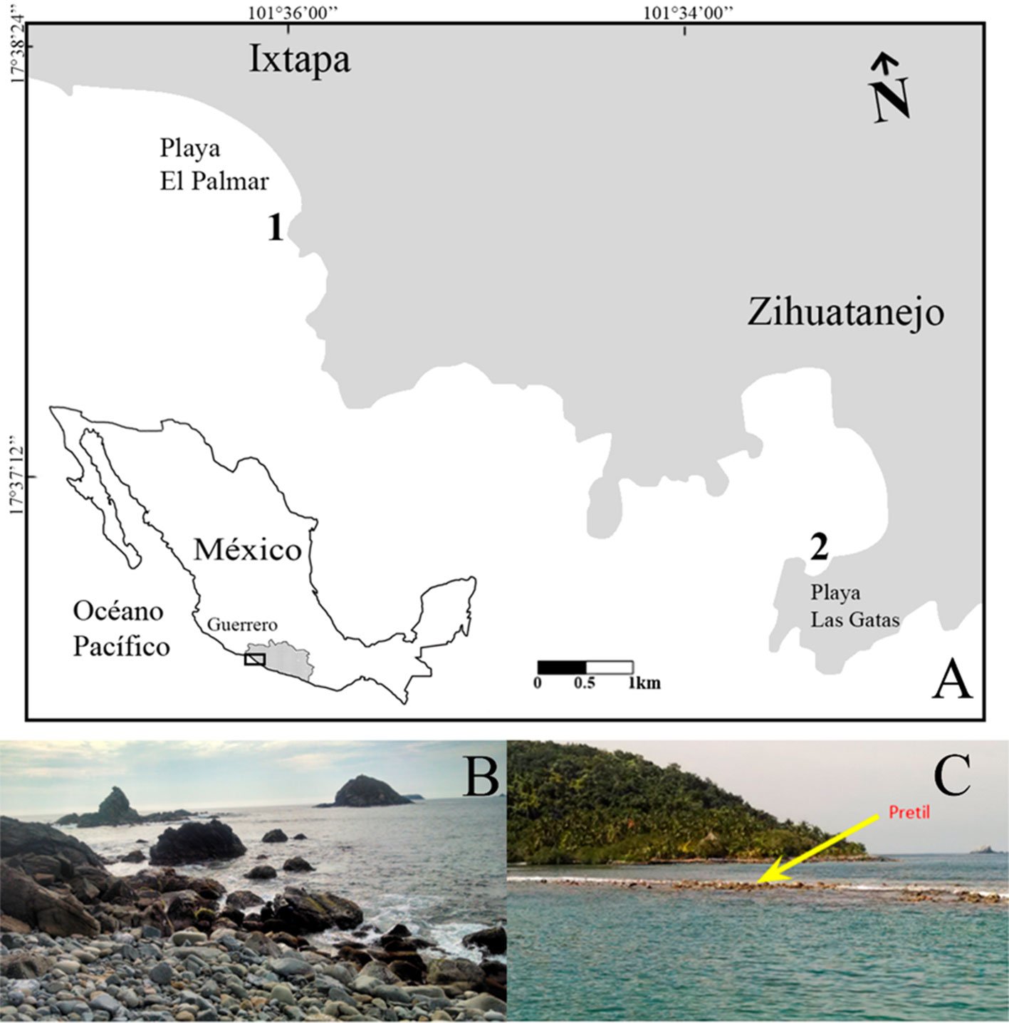
Figura 1. A, Ubicación de la zona de estudio en Ixtapa-Zihuatanejo; B, playa El Palmar; C, playa Las Gatas.
En cada localidad, 3 muestras de macroalgas se recolectaron manualmente de forma aleatoria con una espátula (Bakus, 2007), dentro de cuadros de 20 × 20 cm (0.04 m2) por cada nivel de marea: intermareal bajo (3), medio (3) y alto (3); en total, se obtuvieron 72 muestras provenientes de 36 cuadros en playa Las Gatas y de 36 cuadros en playa El Palmar. Las muestras de las comunidades de macroalgas y moluscos asociados se preservaron en una mezcla de formaldehído al 4% con agua de mar, neutralizada con borato de sodio y glicerina; después se trasladaron al Laboratorio de Ficología (Biodiversidad Marina) de la Facultad de Ciencias de la Universidad Nacional Autónoma de México (UNAM).
En el laboratorio, se calculó la cobertura de cada especie de macroalga en cm2 al colocar cada muestra sobre un área delimitada de 20 × 20 cm. Para su identificación taxonómica se tomaron en cuenta las características morfológicas externas, como tipo de talo y tipo de ramificación, e internas a partir de cortes anatómicos transversales de ejes, frondas y, de estar presentes, de estructuras reproductivas; los especímenes y cortes fueron observados bajo microscopios estereoscópico y óptico (Zeiss). La identificación taxonómica de los ejemplares de macroalgas se realizó utilizando literatura especializada para macroalgas del océano Pacífico (Abbott, 1999; Abbott y Hollenberg, 1976; Dawson, 1949, 1953, 1954, 1960, 1961, 1963; Dawson y Beaudette, 1959; Rodríguez et al.,2008; Taylor, 1945). La actualización de la nomenclatura se hizo a partir de la base de datos de Algaebase (Guiry y Guiry, 2024) y, con base en ella, se elaboró una lista sistemática de las especies de macroalgas. De cada comunidad de macroalgas se separó el sedimento retenido por las algas después de la medición de la cobertura para cada especie y se midió su peso húmedo con una balanza digital, modelo OBI.
De cada muestra, se extrajeron de forma manual todos los moluscos de la clase Bivalvia. Los ejemplares con concha y parte blanda (vivos) fueron identificados al nivel taxonómico más bajo posible, género o especie, dependiendo del estado de conservación de cada ejemplar, a partir de la observación de las características morfológicas de la concha, con apoyo de un microscopio estereoscópico. La identificación taxonómica de las especies se hizo con literatura malacológica especializada para la zona del océano Pacífico oriental (Coan et al., 2000; Keen, 1971). Se elaboró una lista sistemática con base en la propuesta de Bouchet et al. (2010) para los niveles suprafamiliares y la actualización de nomenclatura se realizó a partir de la base de datos de World Register of Marine Species (WORMS) para género y especie (Horton et al., 2024).
Los ejemplares de moluscos y macroalgas recolectados fueron depositados en la colección “Invertebrados asociados a macroalgas”, en proceso de registro, con número de inventario para bivalvos (INV-1531 a INV-1638) del Laboratorio de Ficología (Biodiversidad Marina) de la Facultad de Ciencias, UNAM y las macroalgas se depositaron en la colección del Herbario de la Facultad de Ciencias (FCME) con número de catálogo (PTM-10534 a PTM-10558; PTM-10577 a PTM-10604; PTM-10613 a PTM-10630; PTM-10640 a PTM-10648).
Se elaboró una curva de acumulación de las especies de bivalvos asociados a macroalgas recolectadas en las localidades de estudio, con la finalidad de conocer la cantidad de especies que faltaría encontrar y recolectar en dichas localidades. Con los datos de riqueza de especies (S) y abundancia de bivalvos (N) de ejemplares vivos (concha y parte blanda), se estimaron los índices de Shannon (H´) y de diversidad máxima (H’ max) para cada fecha de muestreo, ya que éstos corresponden a los miembros de la comunidad en el momento de muestreo (Aguilar-Estrada et al., 2014); H´ fue expresado en bits/individuo (Magurran, 2004). Se calculó el índice de equidad de Pielou (J´) y el índice de dominancia de Simpson (D) (Moreno, 2001). Estos índices permiten hacer comparaciones cuantitativas y cualitativas entre estudios o zonas ya que se han utilizado como referente mínimo para describir la estructura comunitaria de un lugar (Aguilar-Estrada et al., 2014).
Para evaluar la normalidad de los datos de abundancia de bivalvos y de los índices de diversidad se realizaron pruebas de Shapiro-Wilk (W) (Siegel, 1990). Posteriormente, se realizaron pruebas de Levene (F) para comprobar la homogeneidad de varianzas para los datos no normales y prueba de Bartlett para los datos con distribución normal (Bartlett, 1937; Levene, 1960). Los índices de diversidad de Shannon fueron analizados usando una prueba de “t de student” para evaluar si existían diferencias estadísticamente significativas entre los meses de muestreo. Estos análisis se realizaron utilizando la paquetería Vegan Versión 2.5-6 (Oksanen et al., 2019) en el programa R Studio 2023.12.0+369 (R Core Team, 2023).
Los datos de abundancia de bivalvos no fueron normales de acuerdo con las pruebas de normalidad, por ello, se realizaron análisis de estadística no paramétrica en el software PRIMER v6 + add on Permanova (PRIMER-E Ltd., Plymouth, UK) (Anderson et al., 2008; Clarke y Gorley, 2006). Los datos fueron transformados con 4√ y con ellos se calculó una matriz de similitud a partir del índice de Bray-Curtis. A partir de dicha matriz, se realizó un análisis de escalamiento multidimensional no métrico (nMDS) con la finalidad de observar la distribución de las abundancias de bivalvos en el área de estudio. Se incluyó la abundancia de las especies dominantes en forma de vectores azules superpuestos en el gráfico nMDS para facilitar la interpretación de las abundancias de especies dominantes en las distintas localidades y niveles de marea, donde el círculo azul representa la variación de la abundancia. Las especies dominantes que se seleccionaron en este análisis son las que estuvieron presentes en todas las muestras con abundancias mayores a la media.
Además, se realizaron análisis de varianza permutacionales (Permanova) para determinar si existían diferencias significativas en la abundancia de bivalvos (variable dependiente) con respecto a los factores utilizados: localidad con 2 niveles (El Palmar y Las Gatas), nivel de marea con 3 niveles (alto, medio y bajo) y mes de muestreo con 4 niveles (enero, mayo, julio y noviembre). En los análisis de Permanova se utilizaron 999 permutaciones de los residuos bajo un modelo reducido. Posteriormente, para los factores donde se obtuvieron diferencias significativas, se realizaron comparaciones de pares para identificar los niveles que eran diferentes estadísticamente (Anderson et al., 2008).
Utilizando las variables numéricas, se realizaron regresiones lineales múltiples con el software SPSS Statistics v20, para evaluar el efecto de la cobertura de macroalgas y los sedimentos retenidos (variables independientes) en la abundancia de bivalvos (variable dependiente) en las playas El Palmar y Las Gatas, en los diferentes niveles de marea y en los meses de muestreo.
Por último, se determinó el grupo morfofuncional (GMF): filamentosas (Fil), foliosas (Fol), foliosas corticadas (Foc), filamentosas corticadas (Fic), coriáceas (Cor), calcáreas articuladas (Cal) para cada especie de macroalgas, con base en la propuesta de Steneck y Dethier (1994) y se asociaron con las especies de bivalvos recolectadas.
Resultados
Riqueza y composición de moluscos. En 60 de las 72 muestras recolectadas se encontraron bivalvos, 35 muestras pertenecientes a playa El Palmar y 25 a playa Las Gatas. Se obtuvieron un total de 873 individuos de la clase Bivalvia. Se identificaron 17 especies (fig. 2) agrupadas en 2 subclases, 8 órdenes, 10 familias y 15 géneros. Del total de especies recolectadas, 2 de ellas Parvilucina approximata (Dall, 1901) y Pinna rugosa G. B. Sowerby I, 1835, encontradas en playa El Palmar y playa Las Gatas, respectivamente, no se incluyeron en los análisis de estructura comunitaria, dado que solo se recolectó la concha. Se obtuvieron 13 especies en playa El Palmar y 9 en playa Las Gatas. Las familias Carditidae y Mytilidae fueron las mejor representadas con 3 (18%) y 5 (30%) especies, respectivamente.
En ambas localidades, las especies más abundantes fueron: Brachidontes adamsianus (Dunker, 1857), Leiosolenus aristatus (Dillwyn, 1817) e Isognomon janus Carpenter, 1857, con 376, 205 y 124 individuos, respectivamente, lo cual representó 91% del total de individuos. Brachidontes adamsianus obtuvo la mayor abundancia en El Palmar a lo largo del ciclo anual, con el valor más elevado (161 individuos) en enero. En Las Gatas, Leiosolenus aristatus fue la especie con la mayor abundanciacon 140 individuos en enero; sin embargo, la especie más abundante fue B. adamsianus a lo largo de los otros meses de muestreo. Mientras que las especies menos abundantes fueron: Sphenia fragilis (H. Adams & A. Adams, 1854) con 2 individuos en enero y mayo en El Palmar y 1 individuo en noviembre en Las Gatas, Crassinella ecuadoriana Olsson, 1961 con 2 individuos en mayo y julio en El Palmar, Linucula declivis (Hinds, 1843) con 2 individuos en julio y noviembre en Las Gatas, Mya sp. y Mytilus edulis Linnaeus, 1758 con 1 individuo en enero en El Palmar (tabla 1).
Tabla 1
Abundancia de las especies de bivalvos recolectadas en las localidades de estudio por mes de muestreo. El arreglo sistemático sigue la propuesta de Horton et al. (2024).
| Especie | Playa El Palmar | Playa Las Gatas | |||||||
| ene | may | jul | nov | ene | may | jul | nov | Total | |
| Subclase Protobranchia | |||||||||
| Orden Nuculida | |||||||||
| Familia Nuculidae | |||||||||
| Linucula declivis | – | – | – | – | – | – | 1 | 1 | 2 |
| Subclase Autobranchia | |||||||||
| Orden Mytilida | |||||||||
| Familia Mytilidae | |||||||||
| Brachidontes adamsianus | 161 | 43 | 18 | 14 | 41 | 9 | 34 | 56 | 376 |
| Brachidontes semilaevis | 4 | – | – | 1 | – | – | – | – | 5 |
| Leiosolenus aristatus | 2 | 30 | 1 | 6 | 140 | 7 | 5 | 14 | 205 |
| Modiolus capax | 1 | 2 | 1 | 1 | – | – | – | – | 5 |
| Mytilus edulis | 1 | – | – | – | – | – | – | – | 1 |
| Orden Arcida | |||||||||
| Familia Arcidae | |||||||||
| Acar rostae | – | – | – | – | – | – | 1 | 3 | 4 |
| Orden Ostreida | |||||||||
| Familia Pteriidae | |||||||||
| Isognomon janus | 51 | 32 | 8 | 5 | 2 | – | 10 | 16 | 124 |
| Familia Pinnidae | |||||||||
| Pinna rugosa | – | – | – | – | – | – | 3 | – | 3 |
| Orden Lucinida | |||||||||
| Familia Lucinidae | |||||||||
| Parvilucina approximata | 1 | – | – | – | – | – | – | – | 1 |
| Orden Carditida | |||||||||
| Familia Carditidae | |||||||||
| Carditamera affinis | 5 | 2 | – | – | 1 | – | – | 1 | 9 |
| Carditamera radiata | – | 3 | 1 | – | 3 | – | 3 | 5 | 15 |
| Cardites grayi | – | 1 | 3 | – | – | – | – | – | 4 |
| Familia Crassatellidae | |||||||||
| Crassinella ecuadoriana | – | 1 | 1 | – | – | – | – | – | 2 |
| Orden Venerida | |||||||||
| Familia Chamidae | |||||||||
| Chama coralloides | 3 | 2 | 1 | – | – | – | – | 7 | 13 |
| Orden Myida | |||||||||
| Familia Myidae | |||||||||
| Mya sp. | 1 | – | – | – | – | – | – | – | 1 |
| Sphenia fragilis | 1 | 1 | – | – | – | – | – | 1 | 3 |
| Total | 231 | 117 | 34 | 27 | 187 | 16 | 57 | 104 | 773 |
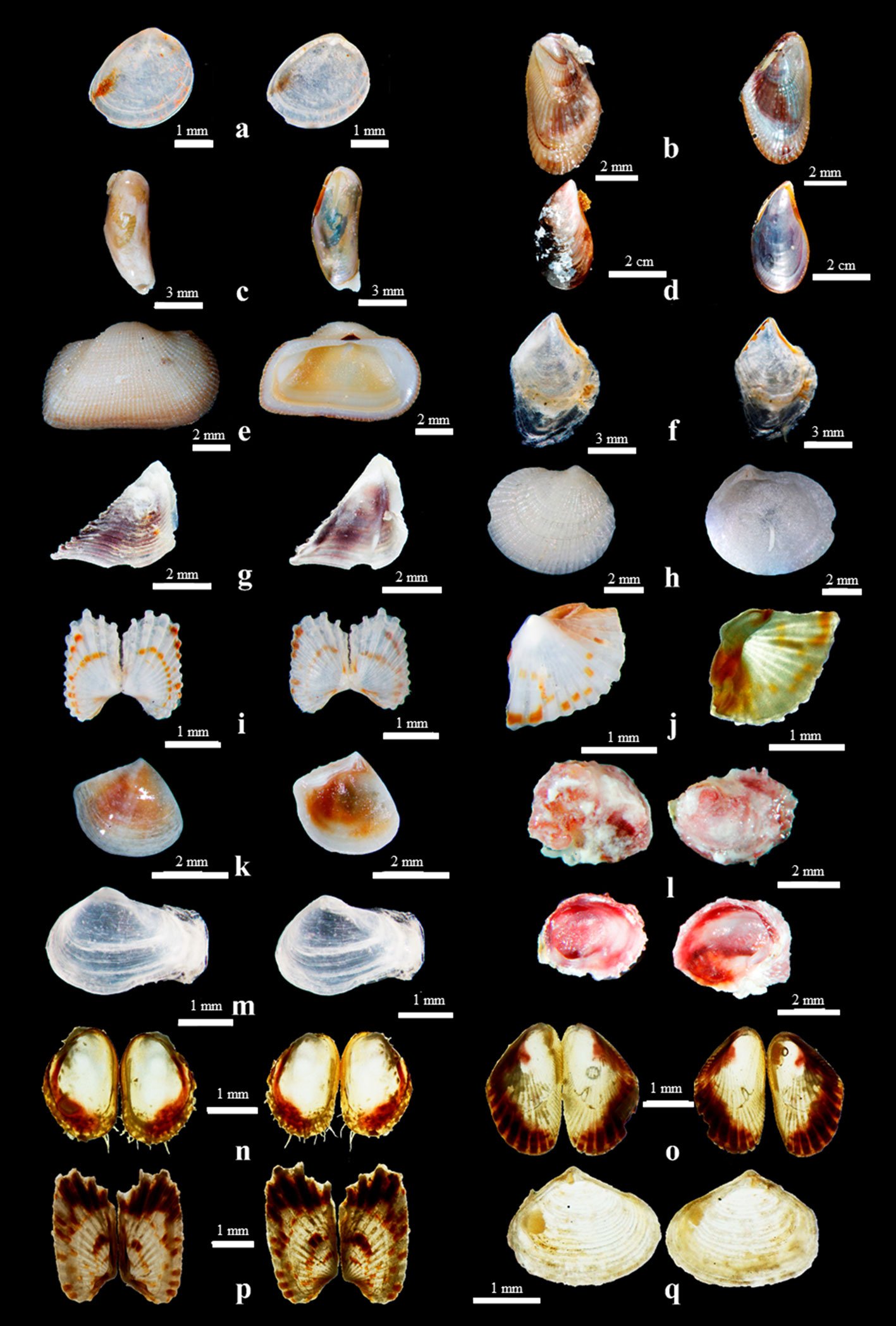
Figura 2. Especies de bivalvos asociadas a macroalgas recolectadas en Ixtapa-Zihuatanejo, Guerrero, en vista dorsal y ventral. a, Linucula declivis;b, Brachidontes adamsianus;c, Leiosolenus aristatus; d, Mytilus edulis; e, Acar rostae; f, Isognomon janus;g, Pinna rugosa; h, Parvilucina approximata; i, Carditamera radiata; j, Cardites grayi; k, Crassinella ecuadoriana; l, Chama coralloides;m, Sphenia fragilis; n, Modiolus capax;o, Brachidontes semilaevis;p, Carditamera affinis;q, Mya sp.
La riqueza de especies con relación al ciclo anual fue de 13 especies en playa El Palmar, variando entre 5 (noviembre) y 10 especies (enero) a lo largo de los meses, mientras que en playa Las Gatas se obtuvieron 9 especies, con una variación de 2 (mayo) y 9 (noviembre) especies (tabla 1). La curva de acumulación de especies mostró un comportamiento asintótico en El Palmar, mientras que Las Gatas no mostró una tendencia a ser asintótica (fig. 3).
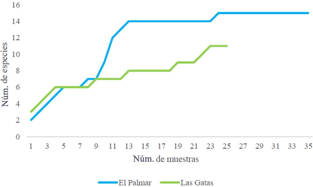
Figura 3. Curva de acumulación de especies de bivalvos registrados en las localidades de estudio. Línea azul: playa El Palmar, línea verde: playa Las Gatas.
En playa El Palmar el nivel intermareal bajo obtuvo el mayor número de especies (13) y el menor número de especies se presentó tanto en el nivel intermareal medio como en el alto (7); mientras que en playa Las Gatas, se presentó el mayor número de especies en el nivel intermareal medio (10) y el nivel alto tuvo el menor número de especies (5). Las especies que se presentaron en ambas localidades en los 3 niveles de la zona intermareal fueron Brachidontes adamsianus, Leiosolenus aristatus e Isognomon janus.
En El Palmar se registraron valores del índice de diversidad de Shannon que fluctuaron entre 1.30 y 2.15 bits/individuo, mientras que en Las Gatas este índice varió entre 0.98 y 2.09 bits/individuo (tabla 2). En general, el índice de equidad de Pielou presentó valores mayores a 0.60 en playa El Palmar, excepto en enero, mientras que en playa Las Gatas se observó que los valores fueron bajos en enero y mayo, y mayores a 0.60 en julio y noviembre. Las pruebas de “t de student”para el índice de diversidad de Shannon entre los meses de muestreo, indicaron diferencias significativas entre todos ellos (p ≤ 0.05) en El Palmar, y Las Gatas (tabla 3).
Tabla 2
Índices comunitarios calculados para las especies recolectadas en playa El Palmar y playa Las Gatas. N = número de individuos, H’= Índice de Shannon, J’= equidad de Pielou y λ = dominancia de Simpson. Los valores máximos y mínimos por localidad para el índice de Shannon (H´) se marcan con negritas.
| Playa El Palmar | Playa Las Gatas | |||||||
| Mes | N | H’ | J’ | λ | N | H’ | J’ | λ |
| Enero | 230 | 1.30 | 0.48 | 0.54 | 187 | 0.99 | 0.41 | 0.60 |
| Mayo | 117 | 2.15 | 0.81 | 0.27 | 16 | 0.98 | 0.41 | 0.50 |
| Julio | 34 | 2.03 | 0.77 | 0.34 | 54 | 1.63 | 0.68 | 0.44 |
| noviembre | 27 | 1.77 | 0.67 | 0.35 | 104 | 2.09 | 0.87 | 0.33 |
En el análisis de escalamiento multidimensional no métrico (nMDS), a partir de los valores de abundancia de las especies de bivalvos, se observó que las muestras se separan en 3 grupos: un primer grupo dominado por estaciones pertenecientes a playa El Palmar (P), un segundo grupo principalmente con estaciones de playa Las Gatas (G) y uno tercero con estaciones de ambas localidades que probablemente se separa por la dominancia de la especie Brachidontes adamsianus (fig. 4). El vector indica la dirección a través del plano de ordenación en la cual aumentan los valores de abundancia de las especies dominantes, la longitud de la línea indica la cantidad de variación total de cada especie, entonces, si toda la variación se explicara, la línea azul alcanzaría el círculo azul.
Tabla 3
Resultado de la prueba de “t de student”para evaluar diferencias significativas del índice de Shannon entre los meses de muestreo por localidad.
| Playa El Palmar | Playa Las Gatas | |||||||
| Meses | H´ | t | p | gl | H´ | t | p | gl |
| enero vs. mayo | 1.30/2.15 | -0.009 | 324 | 1 | 0.99/0.98 | 0.009 | 169 | 1 |
| mayo vs. julio | 2.15/2.03 | 0.0004 | 142 | 0.98/1.63 | -19.84 | 4 | ||
| julio vs. noviembre | 2.03/1.17 | 0.023 | 60 | 1.63/2.09 | -3.18 | 94 |
El análisis de Permanova reveló que la composición de bivalvos difiere significativamente entre las diferentes localidades muestreadas (pseudo-F = 5.2373, p = 0.001). No hubo diferencias estadísticamente significativas para los meses de muestreo (pseudo-F=1.431, p = 0.147) y el nivel de marea (pseudo-F = 1.19, p = 0.309) (tabla 4).
Tabla 4
Resultado de los análisis de Permanova para los factores de localidad, mes de muestreo y nivel de marea. GL: Grados de libertad, ms: media suma de cuadrados, perm: permutaciones, * = valores significativos.
| Factor | GL | ms | Pseudo-F | p (perm) |
| Localidad | 1 | 7,844.9 | 5.2373 | 0.001* |
| Res | 57 | 1,497.9 | ||
| Total | 58 | |||
| Mes | 3 | 2,249.9 | 1.431 | 0.147 |
| Res | 55 | 1,572.3 | ||
| Total | 58 | |||
| Nivel de marea | 2 | 1,915 | 1.1996 | 0.309 |
| Res | 56 | 1,596.3 | ||
| Total | 58 |
Riqueza y composición de macroalgas. Se encontró un total de 3 phyla, 3 clases, 5 subclases, 14 órdenes, 20 familias, 33 géneros y 59 especies de macroalgas; de las cuales, a cada localidad le pertenecen 37 especies. De las 59 especies totales, 11 fueron Chlorophyta (18%), 42 Rhodophyta (70%) y 7 Heterokontophyta-Phaeophyceae (11%). Entre ambas localidades se compartieron 16 especies. Las familias con mayor número de especies fueron Rhodomelaceae con 12 especies, Corallinaceae con 10 y Ceramiaceae y Dictyotaceae con 5 especies cada una (tabla 5).
Asociación entre grupos morfofuncionales y moluscos. Las macroalgas se clasificaron en 6 grupos morfofuncionales: algas filamentosas, foliosas, foliosas corticadas, filamentosas corticadas, coriáceas y calcáreas articuladas (tabla 5). Los grupos dominantes en las 2 localidades fueron las algas filamentosas, filamentosas corticadas y las calcáreas articuladas. En playa El Palmar se presentó una mayor riqueza de especies (14) de bivalvos al interior de las comunidades algales que contenían el grupo de algas calcáreas articuladas. En playa Las Gatas, los grupos morfofuncionales que presentaron mayor cantidad de especies fueron las algas filamentosas, filamentosas corticadas y las calcáreas articuladas con 10 especies cada uno (tabla 6).
Cobertura de macroalgas, abundancia de moluscos y sedimentos retenidos. La regresión lineal por localidad indicó que para playa El Palmar hay una correlación baja con 24% entre los componentes: cobertura de macroalgas, abundancia de bivalvos y peso de sedimento húmedo; sin embargo, se observó una relación moderada entre los sedimentos retenidos por las macroalgas y la abundancia de bivalvos (R = 0.55 y R2 = 0.24). Para playa Las Gatas la regresión lineal múltiple indicó una correlación baja con 10% entre los factores y una relación moderada entre la cobertura de macroalgas y la abundancia de bivalvos (R = 0.42 y R2 = 0.10). La cobertura de macroalgas, abundancia de bivalvos y los sedimentos retenidos varió según la localidad (fig. 5A-C), mes de muestreo (fig. 5D-F) y nivel de marea (fig. 5G-I). En El Palmar la regresión lineal mostró una relación directamente proporcional entre la abundancia de bivalvos y la cobertura de macroalgas. Los valores más altos de cobertura de macroalgas (0.89 m2) se relacionaron con los valores más altos de abundancia de bivalvos.
Con respecto al mes de muestreo, las regresiones lineales múltiples indicaron una correlación alta con 98% (R = 0.99 y R2 = 0.98), entre la cantidad de sedimento retenido y la abundancia de bivalvos. La regresión lineal múltiple sugirió que la abundancia de bivalvos disminuyó a lo largo del ciclo anual, donde enero presentó la mayor abundancia (de 187-230 individuos) y noviembre la menor (27 individuos). La relación de la abundancia de bivalvos con el peso húmedo de sedimento tuvo un comportamiento parecido, disminuyendo conforme al ciclo anual: en las muestras de enero se reportó mayor sedimento retenido (0.56 kg), mientras que en julio se encontraron menos sedimentos retenidos (0.17 kg).

Figura 4. Análisis de escalamiento multidimensional no métrico (nMDS) de las especies de bivalvos recolectadas en las localidades de estudio. Las líneas azules (vectores) indican las especies abundantes y frecuentes (dominantes). El círculo azul representa la variación de las abundancias.
Tabla 5
Especies de macroalgas asociadas a bivalvos, para cada localidad y grupo morfofuncional. Se marca con * la especie de macroalga presente en la localidad. Localidad: playa El Palmar (P), playa Las Gatas (G). Grupos morfofuncionales de macroalgas: filamentosas (Fil), foliosas (Fol), foliosas corticadas (Foc), filamentosas corticadas (Fic), coriáceas (Cor), calcáreas articuladas (Cal). Especies de bivalvos: 1) Linucula declivis, 2) Brachidontes adamsianus, 3) Brachidontes semilaevis, 4) Leiosolenus aristatus, 5) Modiolus capax, 6) Mytilus edulis, 7) Acar rostae, 8) Isognomon janus, 9) Carditamera affinis, 10) Carditamera radiata, 11) Cardites grayi, 12) Crassinella ecuadoriana, 13) Chama coralloides, 14) Mya sp., 15) Sphenia fragilis,16) Pinna rugosa, 17) Parvilucina approximata.
| Especies | Grupo morfofuncional | Especies de bivalvos | |
| P | G | ||
| Chlorophyta | |||
| Ulvales | |||
| Ulvaceae | |||
| Ulva californica Wille, 1899 | Fol | * | – |
| Ulva intestinalis Linnaeus, 1753 | Fol | – | 2, 4, 13 |
| Ulva linza Linnaeus, 1753 | Fol | – | 2, 4, 13 |
| Bryopsidales | |||
| Bryopsidaceae | |||
| Bryopsis pennata var. minor J. Agardh, 1887 | Fil | – | 2, 4, 8 |
| Caulerpaceae | |||
| Caulerpa chemnitzia (Esper) J.V. Lamouroux, 1809 | Fil | 2, 4, 8, 10, 17 | 1, 2, 4, 7, 8, 9, 10, 15 |
| Caulerpa sertularioides (S.G. Gmelin) M. Howe, 1905 | Fil | 2, 4, 8, 10, 17 | 1, 2, 4, 7-10, 15 |
| Halimedaceae | |||
| Halimeda discoidea Decaisne, 1842 | Cal | 2, 10, 17 | – |
| Cladophorales | |||
| Cladophoraceae | |||
| Chaetomorpha antennina (Bory) Kützing, 1847 | Fil | 2, 3, 7, 8-13 | 4, 7, 8, 11, 13 |
| Cladophora sp. | Fil | 2, 4, 5, 8, 9 | – |
| Cladophora graminea Collins, 1909 | Fil | – | 16 |
| Cladophora microcladioides Collins, 1909 | Fil | 2, 4, 5, 8, 9 | – |
| Rhodophyta | |||
| Gigartinales | |||
| Cystocloniaceae | |||
| Hypnea pannosa J. Agardh, 1847 | Fic | 2-6, 8-15 | 2, 4, 8-10, 16 |
| Hypnea spinella (C. Agardh) Kützing, 1847 | Fic | 2-6, 8-15, 17 | 2, 4, 8-10, 16 |
| Hypnea johnstonii Setchell y N. L. Gardner, 1924 | Fic | – | 1, 2, 4, 7-10, 16 |
| Phyllophoraceae | |||
| Ahnfeltiopsis gigartinoides (J. Agardh) P. C. Silva y DeCew, 1992 | Fic | 8 | – |
| Gymnogongrus johnstonii (Setchell y N. L. Gardner) E.Y. Dawson, 1961 | Fic | 2, 8 | – |
| Ceramiales | |||
| Ceramiaceae | |||
| Centroceras clavulatum (C. Agardh) Montagne, 1846 | Fil | 2-5, 8 | 2, 4, 10, 15 |
| Tabla 5. Continúa | |||
| Especies | Grupo morfofuncional | Especies de bivalvos | |
| P | G | ||
| Ceramium sp. | Fil | – | 1, 2, 4, 7, 8, 10, 13, 16 |
| Ceramium camouii E. Y. Dawson, 1944 | Fil | – | 1, 2, 4, 7, 8, 10, 13, 16 |
| Ceramium zacae Setchell y N. L. Gardner, 1937 | Fil | – | 1, 2, 4, 7, 8, 10, 13, 16 |
| Gayliella flaccida (HarveyyKützing) T.O. McIvory y L.J. Cho, 2008 | Fic | – | 2, 4, 7, 8, 11 |
| Delesseriaceae | |||
| Taenioma perpusillum (J. Agardh) J. Agardh, 1863 | Fil | – | 4, 16 |
| Rhodomelaceae | |||
| Chondria sp. | Fic | * | * |
| Herposiphonia secunda (C. Agardh) Ambronn, 1880 | Fic | 8 | 2, 4, 8, 10 |
| Herposiphonia tenella (C. Agardh) Ambronn, 1880 | Fic | 7 | – |
| Melanothamnus simplex (Hollenberg) Díaz-Tapia y Maggs, 2017 | Fic | 2, 8 | – |
| Melanothamnus sphaerocarpus (Borgesen) Díaz.Tapioa y Maggs, 2017 | Fic | – | 2, 4, 8 |
| Polysiphonia mollis J. D. Hooker y Harvey, 1847 | Fic | * | 2, 4, 8, 15 |
| Polysiphonia nathanielii Hollenberg, 1958 | Fic | – | 2, 4, 8, 15 |
| Polysiphonia subtilissima Montagne, 1840 | Fic | – | 2, 4, 8, 15 |
| Eutrichosiphonia confusa (Hollenberg) Savoie y G.W. Saunders, 2019 | Fic | – | 2, 4, 8 |
| Laurencia sp. | Fic | 2, 8, | 2, 7, 8, 13 |
| Laurencia hancockii E.Y. Dawson, 1944 | Fic | 2, 8 | – |
| Laurencia subcorymbosa E.Y. Dawson, 1963 | Fic | 2, 8 | – |
| Rhodymeniales | |||
| Rhodymeniaceae | |||
| Tayloriella dictyurus (J. Agardh) Kylin, 1956 | Fil | 2, 8 | – |
| Lomentariaceae | |||
| Ceratodictyon tenue (Setchell y N. L. Gardner) J.N. Norris, 2014 | Fil | – | 2, 4, 8 |
| Corallinales | |||
| Corallinaceae | |||
| Amphiroa beauvoisii J.V. Lamouroux, 1816 | Cal | 2-15, 17 | 1, 2, 4, 7-14, 16 |
| Amphiroa misakiensis Yendo, 1902 | Cal | 2-15 | 1, 2, 4, 7-14, 16 |
| Amphiroa rigida J.V. Lamouroux, 1816 | Cal | 2-15 | 1, 2, 4, 7-14, 16 |
| Amphiroa subcylindrica E.Y. Dawson, 1953 | Cal | 2-15 | – |
| Jania capillacea Harvey, 1853 | Cal | – | 2, 4, 7-10, 15, 16 |
| Jania subpinnata E.Y. Dawson, 1953 | Cal | 2, 4, 5, 8, 9, 12, 14 | 2, 4, 7-10, 15, 16 |
| Jania tenella (Kützing) Grunow, 1874 | Cal | 2, 4, 5, 8, 9, 12, 14 | 2, 4, 7-10, 15, 16 |
| Jania tenella var. tenella | Cal | 2, 4, 5, 8, 9, 12, 14 | – |
| Gelidiales | |||
| Gelidiaceae | |||
| Gelidiella acerosa (Forsskal) Feldmann y Hamel, 1934 | Fic | – | 2, 7, 8 |
| Gelidium mcnabbianum (E.Y. Dawson) B. Santelices, 1998 | Fic | – | 2, 4, 7-11 |
| Gelidium pusillum (Stackhouse) Le Jolis, 1863 | Fic | 2, 4, 5, 8, 12, 14 | 2, 4, 7-11 |
| Pterocladiaceae | |||
| Pterocladiella caloglossoides (M. Howe) Santelices, 1998 | Fic | – | 2, 4, 7, 8, 15 |
| Gracilariales | |||
| Gracilariaceae | |||
| Gracilaria sp. | Fic | 2, 8, 12, 14 | – |
| Halymeniales | |||
| Halymeniaceae | |||
| Grateloupia huertana Mateo-Cid, Mendoza-González y Gavio, 2005 | Fic | – | 4, 8 |
| Grateloupia versicolor (J. Agardh) J. Agardh, 1847 | Fic | 2, 4, 8 | – |
| Heterokontophyta-Phaeophyceae | |||
| Ectocarpales | |||
| Scytosiphonaceae | |||
| Chnoospora minima Papenfuss, 1956 | Fic | * | – |
| Fucales | |||
| Sargassaceae | |||
| Sargassum liebmannii Agardh, 1847 | Cor | 2, 4, 5, 7, 8, 10-13, 15, 17 | – |
| Dictyotales | |||
| Dictyotaceae | |||
| Dictyota sp. | Foc | – | * |
| Dictyota dichotoma (Hudson) J.V. Lamouroux, 1809 | Foc | 2, 4, 5, 8 | – |
| Lobophora variegata (J.V.Lamouroux)Womersley ex E.C.Oliveira, 1977 | Fic | 8 | – |
| Padina mexicana var. erecta Avila-Ortiz, 2003 | Foc | 2, 4, 5, 8, 9 | – |
| Padina ramonribae Avila-Ortiz, Pedroche y Díaz-Martínez, 2016 | Foc | 2, 4, 5, 8, 9 | – |
La regresión lineal por nivel de marea indicó una correlación significativa con 100% (R = 1 y R2 = 1), es decir, la cobertura de algas y el sedimento retenido están relacionados con la abundancia de bivalvos en los diferentes niveles de marea. El nivel del intermareal bajo presentó los valores más elevados de cobertura de macroalgas con 0.61 m2 (fig. 5G), mayor abundancia de moluscos con 275 individuos (fig. 5H) y mayor cantidad de sedimentos con 0.69 kg (fig. 5I). En el intermareal alto se registraron los valores más bajos de abundancia de bivalvos con 230 individuos (fig. 5H), cobertura de algas con 0.52 m2 (fig. 5G) y peso húmedo de sedimentos con 0.30 kg (fig. 5I), es decir, conforme se asciende en el intermareal, estas variables disminuyen.
Tabla 6
Asociación de las especies de bivalvos con los grupos morfofuncionales propuestos por Steneck y Dethier (1994). Grupos morfofuncionales de macroalgas: filamentosas (Fil), foliosas (Fol), foliosas corticadas (Foc), filamentosas corticadas (Fic), coriáceas (Cor), calcáreas articuladas (Cal). × = Presencia de la especie.
| Familia | Especie | Playa El Palmar | Playa Las Gatas | ||||||||||
| Fil | Fol | Foc | Fic | Cor | Cal | Fil | Fol | Foc | Fic | Cor | Cal | ||
| Nuculidae | L. declivis | – | – | – | – | – | – | × | – | – | × | – | × |
| Mytilidae | B. adamsianus | × | – | × | × | × | × | × | × | – | × | – | × |
| B. semilaevis | × | – | – | × | – | × | – | – | – | – | – | – | |
| L. aristatus | × | – | × | × | × | × | × | × | – | × | – | × | |
| M. capax | × | – | × | × | × | × | – | – | – | – | – | – | |
| M. edulis | – | – | – | × | – | × | – | – | – | – | – | – | |
| Arcidae | A. rostae | × | – | – | – | × | × | × | – | – | × | – | × |
| Pteriidae | I. janus | × | – | × | × | × | × | × | – | – | × | – | × |
| Pinnidae | P. rugosa | – | – | – | – | – | – | × | – | – | × | – | × |
| Lucinidae | P. approximata | × | – | – | × | × | × | – | – | – | – | – | – |
| Carditidae | C. affinis | × | – | × | × | – | × | × | – | – | × | – | × |
| C. radiata | × | – | – | × | × | × | × | – | – | × | – | × | |
| C. grayi | × | – | – | × | × | × | × | – | – | × | – | × | |
| Crassatellidae | C. ecuadoriana | × | – | – | × | × | × | – | – | – | – | – | – |
| Chamidae | C. coralloides | × | – | – | × | × | × | × | × | – | × | – | × |
| Myidae | Mya sp. | – | – | – | × | – | × | – | – | – | – | – | – |
| S. fragilis | – | – | – | × | × | × | × | – | – | × | – | × | |
| Total | 12 | 0 | 5 | 14 | 11 | 15 | 11 | 3 | 0 | 11 | 0 | 11 |
Discusión
Riqueza y composición de moluscos. De las 17 especies encontradas en el presente estudio, 16 ya habían sido observadas para el Pacífico tropical mexicano, específicamente para Ixtapa-Zihuatanejo en sustratos rocosos y arenosos (Flores-Rodríguez et al., 2007, 2012; Lesser, 1984; López-Rojas et al.,2017; Lozada, 2010; Sánchez, 2014), excepto Mytilus edulis que es un nuevo registro para Guerrero. Esta especie fue encontrada en playa El Palmar, asociada a los géneros de macroalgas Amphiroa e Hypnea. Dicha especie había sido registrada para el océano Pacífico desde las costas del Ártico, Canadá, EUA, hasta Cabo San Lucas, México, al interior del golfo de California en San Luquitas y Santa Rosalía, y para el Pacífico tropical mexicano en isla Socorro, por lo que su distribución se amplía hacia el sur, a Guerrero en ambientes litorales asociados a las comunidades de macroalgas (Cadena-Cárdenas et al., 2009; Fitch, 1953; Shaw et al., 1988). La ampliación de la distribución de esta especie puede deberse al movimiento de la corriente de California como ha sido reportado para bivalvos (Schulien et al., 2020), gasterópodos y escafópodos que ampliaron su distribución desde la provincia Californiana hacia la Panámica donde se señala la confluencia de especies de moluscos entre ambas provincias (Landa-Jaime y Arciniega-Flores 1998; Ríos-Jara et al., 2003; Gama-Kwick et al., 2021). Otra de las razones por la cual M. edulis amplió su distribución al sur podría ser por el fenómeno de El Niño que proporciona condiciones ambientales para que las especies que habitan en sitios templados y subtropicales se desplacen a sitios tropicales (Díaz y Ortlieb, 1993; Paredes et al., 1998; Velez y Zeballos, 1985).

Figura 5. Variación de cobertura de macroalgas, abundancia de bivalvos y sedimento retenido por localidades (A, B y C), mes de muestreo (D, E y F) y nivel de la zona intermareal (G, H e I). Verde = macroalgas, amarillo = bivalvos, rojo = sedimento retenido.
La familia mejor representada fue Mytilidae con 5 especies: Brachidontes adamsianus, B. semilaevis, Leiosolenus aristatus, Modiolus capax y Mytilus edulis (tabla 1), dichas especies coinciden con lo registrado por Flores-Garza et al.(2014), Galeana-Rebolledo et al.(2012) y Garcés (2011) en Acapulco, así como por López-Rojas et al. (2017) en diferentes localidades en Guerrero. Mytilidae también ha sido la familia mejor representada en otras localidades de Zihuatanejo (muelle municipal), donde se han observado 8 especies (Guzmán, 2022), así como en otras regiones tropicales como Brasil, donde esta familia también fue la mejor representada con 5 especies (Santos et al., 2020).
Una mayor riqueza de especies de la familia Mytilidae en Ixtapa-Zihuatanejo podría explicarse debido a la frecuencia y rápido asentamiento de larvas de bivalvos, ya que son organismos que están en constante reproducción a lo largo del año (Seed, 1969a). Suchanek (1978) mencionó que los miembros de la familia Mytilidae tienden a colonizar rápidamente los espacios disponibles en la zona intermareal rocosa, familia que se ha adaptado a distintos hábitats (Keen, 1971), gracias a su rápido aumento de talla y posterior asentamiento de larvas (Ceccherelli y Rossi, 1984). También se ha mencionado que los organismos de dicha familia pueden producir fibras de biso, por lo que son capaces de anclarse y permanecer en sustratos en los que otras familias de bivalvos no pueden, como rocas, arenas u otros organismos (Keen, 1971; Stella et al.,2010).
En general, se encontró una mayor riqueza de especies en El Palmar, valores que pueden explicarse debido a la heterogeneidad ambiental de una playa expuesta con oleaje intenso como dicho sitio (Morales et al., 2008). Se ha mencionado que la riqueza de especies de bivalvos es mayor en zonas expuestas en donde las olas impactan directamente, por su parte, las zonas protegidas o de menor oleaje presentan menor riqueza específica (Flores-Garza et al., 2014; Flores-Rodríguez et al., 2012; Valdés-González et al., 2004).
En El Palmar, se encontraron valores elevados para la riqueza de especies de bivalvos (17 spp.) respecto de lo encontrado en Las Gatas, lo anterior también se ha observado para otras clases de moluscos como los gasterópodos y poliplacóforos asociados a comunidades de macroalgas en playa El Palmar (Aguilar, 2017). También en esta playa se encontró menor cantidad de sedimentos retenidos por las macroalgas (fig. 5C). El Palmar está conformada por rocas de diferentes tamaños, que pueden moverse conforme se dan los cambios en el oleaje y la marea, lo que le confiere un alto dinamismo que no permite la acumulación de sedimentos (Gibbons, 1988), tal como se observó en el presente estudio. Dichas características ayudan a que se conformen una amplia gama de ambientes que pueden ser colonizados, donde se esperaría una mayor riqueza de especies como se observó para los bivalvos de El Palmar (Benedetti-Cecchi, 2001).
Como se ha mencionado anteriormente, playa Las Gatas es un sitio protegido, por esta razón es un lugar de baja energía, con características poco favorables para el establecimiento de especies de bivalvos de manera muy similar a los estudios realizados en otras zonas de Guerrero (Flores-Garza et al., 2014; Flores-Rodríguez et al., 2012; Valdés-González et al., 2004). Las fluctuaciones observadas entre ambas playas de la riqueza de especies, también podrían deberse a otro tipo de características presentes en algunas familias de bivalvos que no tienen hábitos epifaunales como los que se adhieren a las macroalgas y que presentan hábitos de vida semiinfaunales o infaunales (Garcés, 2011), por lo que estas especies podrían encontrarse en otros sitios, posiblemente en zonas más profundas en la zona submareal, o de igual forma, las especies de bivalvos se pueden ver afectadas por la contaminación al incorporar en sus tejidos bacterias patógenas (Gosling, 2015), que es común de una zona turística como Ixtapa-Zihuatanejo (IMTA, 2010; UNAM, 2013). Lo anterior podría explicar las fluctuaciones en la riqueza de especies de bivalvos observadas en Zihuatanejo.
Los valores de riqueza de especies no variaron considerablemente en las localidades estudiadas a lo largo del año. La riqueza de especies de bivalvos en un ciclo anual puede ser constante, ya que la mayoría de las especies (70%) de bivalvos del presente trabajo son generalmente inmóviles o sedentarias. Lo anterior hace que sus poblaciones se mantengan con pocos cambios con respecto a su riqueza de especies debido a sus patrones de reproducción anuales o bianuales (Baqueiro y Masso, 1988; Flores-Rodríguez et al., 2012; Seed, 1969a).
La especie más abundante en el presente trabajo fue B. adamsianus (Mytilidae). Esta especie ha sido registrada como la más abundante en otras localidades de Zihuatanejo (Guzmán, 2022). En particular, las familias Chamidae y Mytilidae se han registrado como las más abundantes para Guerrero; por su parte, la especie Isognomon janus Carpenter, 1857 (Isognomonidae) también ha presentado un gran número de organismos (Guzmán, 2022; López-Rojas et al. 2017). Las bajas abundancias de los bivalvos encontrados en este trabajo pueden estar dadas por el tipo de hábitos de vida de dichos moluscos. Por ejemplo, el género Sphenia tienen un hábito endolítico (Esqueda-González et al., 2014; Garcés, 2011; Guzmán, 2022), por lo que sería poco probable encontrarlos dentro de las comunidades de macroalgas, ya que es común encontrarlos incrustados en agujeros preexistentes de rocas, fragmentos de madera, incluso otros materiales como las conchas de moluscos, así como entre colonias de briozoos (Coan, 1999). El Permanova mostró que existen diferencias significativas entre localidades, esto puede deberse a que playa Las Gatas es considerada como un sitio protegido y playa El Palmar como un sitio expuesto, esto representó diferencias en abundancia y riqueza de especies, que pueden deberse a los requerimientos medioambientales propios de cada una de las especies de bivalvos como: sustrato, alimento, salinidad o temperatura (Borges et al., 2014; Galeana-Rebolledo et al., 2012; Seed 1969a).
En playa El Palmar, la curva de acumulación de especies fue asintótica, lo que sugiere que se encontró a la mayoría de los bivalvos asociados a macroalgas de esta localidad. Mientras que, en playa Las Gatas, la curva de acumulación de especies no fue asintótica. La cantidad de especies recolectadas en un sitio está relacionada con el esfuerzo de muestreo (Moreno, 2001). Por lo que el menor número de muestras en donde se encontraron bivalvos en playa Las Gatas (25), en comparación con las de playa El Palmar (35), podría explicarse por este hecho. Se ha mencionado que una curva de acumulación de especies en muy raras ocasiones llega a ser asintótica, ya que siempre habrá especies que no se recolecten o durante los muestreos pueden encontrarse especies raras, lo que puede estar determinado por el sitio de muestreo, temporada del año, tipo de sustrato, entre otras variables (Jiménez-Valverde y Hortal, 2003).
Además, otra de las razones para que la curva de acumulación de especies no haya sido asintótica para Las Gatas, podría deberse a que, en ambas localidades, las muestras de bivalvos fueron obtenidas de comunidades de macroalgas, que es un sustrato muy específico y es distinto a las rocas y arena que componen la zona intermareal que corresponden a los sustratos que se han estudiado en la mayoría de los distintos trabajos malacológicos de Guerrero. Por lo anterior, el inventario podría estar incompleto; sin embargo, es una buena aproximación de la biodiversidad de las especies de bivalvos asociadas a comunidades de macroalgas de la zona norte de Guerrero en Ixtapa-Zihuatanejo. Para tener una curva de acumulación de especies asintótica se recomienda muestrear todos los sustratos posibles y de esta forma, obtener casi todas las especies de bivalvos de la zona.
Se encontraron cambios con respecto a la abundancia de bivalvos asociados a macroalgas a lo largo del año, fluctuaciones que pudieran estar relacionadas con sus patrones reproductivos, lo que podría explicar la disminución en la abundancia de bivalvos en los meses cálidos (mayo y julio) y un aumento en la cantidad de individuos en los meses fríos (enero y noviembre). Los cambios en la abundancia de bivalvos se han estudiado en trabajos sobre reproducción de diferentes especies de moluscos (Baqueiro y Aldana, 2000, 2003). Algunas de las especies de bivalvos que han sido utilizadas en estudios reproductivos o sobre ciclos gonádicos son: Chione undatella (G. B. Sowerby I, 1835), Megapitaria aurantiaca (G. B. Sowerby I, 1831) (Veneridae), Brachidontes rodriguezii (d’Orbigny, 1842), Mytilus edulis y Mytilus chilensis Hupé, 1854 (Mytilidae), así como Anadara tuberculosa (G. B. Sowerby I, 1833) (Arcidae), tanto en México como otros países de Sudamérica. Dichos estudios destacan que los bivalvos se reproducen continuamente a lo largo del año y se ha mencionado que el momento del desove comprende desde la primavera hasta el otoño con temperaturas por encima de los 25 °C; se ha observado que las larvas se instalan en octubre y noviembre, con una metamorfosis de 15 a 25 días, dichas larvas permanecen adheridas a las algas de noviembre a mayo, en donde llevan a cabo su metamorfosis (Aguillón, 2011; Baqueiro y Masso, 1988; García-Domínguez et al., 2008; Hernández-Moreno et al., 2020; Oyarzún et al., 2011; Seed, 1969a; Torroglosa, 2015). Solo se encontró a Mytilus edulis como especie de importancia comercial para el presente trabajo. En especies que no se les ha considerado importantes para la industria pesquera, es muy poco lo que se conoce acerca de sus hábitos reproductivos (Aguilar, 2017).
Las 3 especies más abundantes del presente trabajo son epifaunales de hábitos filtradores por suspensión (García-Cubas, 1981), Isognomon janus (Isognomonidae) habita en la zona intermareal hasta profundidades de 20 m, Leiosolenus aristatus (Mytilidae)puede encontrarse desde el litoral hasta los 300 m sobre rocas u otros bivalvos (Coan y Valentich-Scott, 2012) y Brachidontes adamsianus (Mytilidae)habita sobre grietas de rocas grandes en zonas expuestas (Landa-Jaime et al., 2013). Las especies que no pertenecen a las familias Isognomonidae y Mytilidae, en general, son organismos infaunales de hábitos filtradores por suspensión, a excepción de la familia Myidae que son infaunales perforadores de hábitos filtradores por suspensión (García-Cubas, 1981; Coan, 1999).
Los bivalvos están presentes en diferentes lugares al interior de la zona intermareal rocosa y hay especies que tienen preferencia por algún sitio a lo largo de dicha zona (Román-Contreras et al.,1991; Sibaja-Cordero y Vargas-Zamora, 2006; Suchanek, 1978). En el presente estudio se observó un incremento en la abundancia y riqueza en los niveles intermareales medio y bajo. Este mismo patrón se ha observado en otras especies de moluscos como gasterópodos y poliplacóforos de Zihuatanejo (Aguilar, 2017; Gama-Kwick et al., 2021).
El índice de diversidad de Shannon obtenido en este trabajo fue bajo, menor a 2.16 bits/individuo para ambos sitios de muestreo, en comparación con otros trabajos sobre bivalvos asociados a macroalgas para Zihuatanejo, como el de Guzmán (2022), donde se encontraron valores de 3.41 bits/individuo en el muelle municipal. Flores-Garza et al.(2014), en su estudio en Acapulco, presentaron valores de 3.65 bits/individuo y Galeana-Rebolledo et al.(2012) reportaron valores de 3.64 bits/individuo. Las diferencias con respecto al índice de diversidad de Shannon pueden deberse a la baja riqueza de especies encontrada en Ixtapa-Zihuatanejo, respecto de otras localidades del Pacífico tropical mexicano, donde se han registrado valores superiores a 17 especies; Reguero y García-Cubas (1989) encontraron 53 especies de bivalvos para Nayarit, y Esqueda-González et al. (2014) reportaron 89 especies de bivalvos para Sinaloa. Lo anterior también puede relacionarse con los altos valores de abundancia de ciertas especies, como es el caso de Brachidontes adamsianus. Ésto también se ve reflejado en los valores calculados del índice de dominancia de Simpson, el cual dio como resultado valores moderados, ya que la abundancia de las especies de bivalvos no es homogénea a lo largo de la zona intermareal rocosa en ambas localidades del presente estudio.
Garcés (2011), describió valores similares del índice de diversidad de Shannon para especies de bivalvos en sustratos rocosos en Acapulco (2.41 bits/individuo) y mencionó que éstos varían según el tipo de sustrato, ya que la riqueza de especies fue mayor en sustratos arenosos que en sustratos rocosos, lo que ocasiona que en estos sustratos, los valores disminuyan.
En el nMDS se observan 3 agrupaciones: una con muestras de la localidad de playa El Palmar, otra con estaciones de playa Las Gatas y la tercera con estaciones de ambas localidades, donde solamente hubo presencia de la especie Brachidontes adamsianus (tabla 1). Dicha especie es una de las más comunes en varias localidades de Jalisco, Oaxaca y Guerrero, por lo que sus valores de abundancia en Ixtapa-Zihuatanejo concuerdan con lo encontrado en otras contribuciones (Castro-Mondragón et al., 2016; Galeana-Rebolledo et al., 2012; Garcés, 2011; Holguín-Quiñones y González-Pedraza 1989; Landa-Jaime et al., 2013; López-Rojas et al., 2017; Torreblanca-Ramírez et al., 2012).
Asociación entre grupos morfofuncionales y moluscos. Los bivalvos recolectados tuvieron una mayor presencia en el grupo morfofuncional de algas filamentosas en ambas localidades, este mismo resultado se observó en muelle municipal en Zihuatanejo por Guzmán (2022) para los bivalvos asociados a macroalgas. Lo anterior puede verse favorecido porque este grupo de algas proporciona refugio ante el oleaje y la desecación, de igual forma tienen un papel fundamental en el asentamiento de las larvas de bivalvos, ya que son utilizadas como un sitio para evitar la competencia entre estadios juveniles y adultos (Dobretsov, 1999; Seed, 1969a).
Las larvas de la familia Mytilidae son atraídas hacia los filamentos de algas rojas de los géneros Ceramium y Polysiphonia, en donde llevan a cabo su metamorfosis (Seed, 1969a), ambos géneros fueron encontrados en el presente trabajo. Las especies de bivalvos de la familia Mytilidae también se encontraron junto con otros géneros de macroalgas como: Bryopsis, Caulerpa, Chaetomorpha y Cladophora (Chlorophyta), dichos géneros también se han relacionado a comunidades de bivalvos en el Caribe colombiano (Quirós-Rodríguez y Campos, 2013). Los géneros Gayliella, Herposiphonia, Taenioma y Tayloriella (Rhodophyta) también se han observado junto a especies de bivalvos, en particular el género Tayloriella se ha encontrado vinculado a 9 diferentes especies de bivalvos en el muelle municipal en Zihuatanejo (Guzmán, 2022). Aun cuando es poco lo que se conoce sobre las asociaciones de bivalvos con macroalgas, es posible sugerir que las larvas de las otras familias de bivalvos encontradas en el presente trabajo (Arcidae, Carditidae, Crassatellidae, Chamidae, Myidae y Pteriidae) puedan tener un comportamiento similar al de Mytilidae y, por esta razón, se podría reconocer su presencia en las comunidades de macroalgas.
La asociación de las especies de bivalvos (B. adamsianus, B. semilaevis, L. aristatus, M. capax, M. edulis, A. rostae, I. janus, C. affinis, C. radiata, C. grayi, C. ecuadoriana, C. coralloides, Mya sp. y S. fragilis) con el grupo de algas filamentosas corticadas fue explicado para especies del género Gigartina porSeed (1969a), quien afirmó que este tipo de algas proporciona una mayor protección y partículas de sedimento retenido (alimento), comparado con las algas filamentosas. En el presente trabajo se encontraron especies de los géneros Ceratodyction, Gelidiella, Gelidium, Gracilaria e Hypnea, que podrían tener una relación similar a la dada por las especies de Gigartina, ya que comparten el mismo grupo morfofuncional propuesto por Steneck y Dethier (1994).
Todas las especies de bivalvos se asociaron al grupo de algas calcáreas articuladas. Las especies del género Corallina proporcionan condiciones ambientales adecuadas para los bivalvos como: refugio, captación de partículas y cantidad de CaCO3 (Seed, 1969a). De esta forma, los bivalvos son capaces de alcanzar tallas mayores en menor tiempo (Seed, 1969a, b). Probablemente, la cantidad de CaCO3 obtenida del ambiente por las macroalgas, queda disponible para que los bivalvos la aprovechen, una vez que las macroalgas mueren. En el presente trabajo, se observó a las especies de algas calcáreas articuladas de los géneros Amphiroa, Halimeda y Jania asociadas a las especies de bivalvos son muy similares a las del género Corallina y comparten el mismo grupo morfofuncional, por lo que podrían funcionar de la misma forma al ser algas que pueden fijar CaCO3 y ser una fuente de aprovechamiento para otros organismos; estas algas calcáreas son la fuente principal de carbonatos marinos (Feely et al., 2004).
Cobertura de macroalgas, abundancia de moluscos y sedimento retenido. La cobertura de macroalgas, abundancia de bivalvos y sedimento retenido disminuyeron conforme se aumentó el nivel del intermareal, los valores más elevados para dichas variables se observaron en el nivel del intermareal bajo (fig. 5G-I). Los resultados de la regresión lineal múltiple sustentan lo anterior, ya que se encontró una relación entre la cobertura de macroalgas y abundancia de bivalvos. Lo anterior podría explicarse por las características del terreno (emersión), debido a que, en un ambiente cambiante como la zona intermareal rocosa, las macroalgas quedan expuestas a una mayor radiación solar en el nivel alto. Por lo tanto, al haber menos céspedes algales (Huovinen et al., 2006), la retención de sedimento es baja, estos 2 factores influyen en las necesidades de cada especie de bivalvo, lo que determina la supervivencia de estos moluscos en esta zona (Airoldi, 2003; Rosenberg, 1977).
Renaud et al. (1997) encontraron una relación entre la abundancia de macroalgas con respecto al sedimento, donde la cobertura de macroalgas era sistemáticamente mayor en las zonas con baja cantidad de sedimentos y un aumento notable en la abundancia de macroalgas se observó después de la remoción de sedimentos. Esto se relaciona con lo encontrado en el presente trabajo, donde se observó una menor cobertura de macroalgas asociada a valores elevados de sedimento. Con respecto de los bivalvos, Forster y Zettler (2004) observaron que la biomasa de Mya arenaria Linnaeus, 1758 se redujo con la presencia de sedimentos finos, lo que podría sugerir que en playa Las Gatas existe una menor abundancia de bivalvos (Airoldi, 2003).
El sedimento en las comunidades de macroalgas queda retenido ya que se acumula en los espacios que hay entre los talos; las cantidades de sedimento acumuladas pueden estar determinadas por la complejidad estructural del alga y las condiciones del medio (García, 2009). La variación en la tasa de sedimentación podría ser un factor de alteración y estrés sobre las comunidades de macroalgas, lo que ocasiona que la tasa de crecimiento algal se vea reducida por la falta de incidencia de luz. Por ello, la fauna que ahí se establece, como las especies de bivalvos, también es menor, ya que una gran cantidad de sedimentos retenidos provoca que los organismos puedan sofocarse y el reclutamiento larval se vea reducido (Airoldi, 2003; Rosenberg, 1977). La clase Bivalvia tiene una preferencia por sustratos arenosos, rocosos, lodosos y fangosos, sin embargo, cuando los sitios no tienen corrientes fuertes y la acumulación de sedimento es alta, la abundancia de bivalvos baja drásticamente (Gosling, 2015).
Las larvas de bivalvos se instalan sobre las algas, donde permanecen adheridas a ellas y llevan a cabo su metamorfosis entre 15 y 25 días; en este lapso, los céspedes algales les proporcionan alimento por el sedimento que retienen y protección contra depredadores y factores abióticos. Posteriormente, los bivalvos juveniles migran fuera de las algas ya que han alcanzado una talla óptima o las algas ya no les brindan suficientes recursos, y llegan a otro sitio que será el definitivo para llevar a cabo el resto de su ciclo de vida (Seed, 1969a, 1969b; Suchanek, 1978).
Olafsson (1986) encontró una relación significativa entre la abundancia de bivalvos y el sedimento, estos resultados son consistentes con lo encontrado en el presente estudio en Ixtapa-Zihuatanejo. Sin embargo, Vázquez (2009) en playa Las Gatas no encontró relación entre la riqueza de especies y el sedimento retenido. Por su parte, en playa El Palmar, que es una zona expuesta, una posible explicación para la relación entre abundancia de bivalvos y sedimento es debido al tipo de hábitos de vida de la mayoría de las especies encontradas en el presente trabajo, ya que la mayoría de ellas son epifaunales o infaunales con hábitos filtradores suspensívoros. La erosión del sustrato rocoso por la acción de las olas y por el movimiento de los sedimentos puede generar heterogeneidad ambiental (Airoldi, 2003). La mezcla constante del agua provee mayor humedad, así como nutrientes al suspender los sedimentos, lo que ocasiona una mayor supervivencia de los organismos, lo que explicaría la relación entre abundancia y sedimento (Gama-Kwick et al., 2021).
Las condiciones de playa El Palmar con un oleaje intenso (Morales et al., 2008), no permite la retención de sedimentos, su baja cantidad podría influir en la composición de las macroalgas. Por lo tanto, la composición de los invertebrados al interior de éstos puede ser muy particular en esta localidad (Gama-Kwick et al., 2021), lo que puede incrementar su diversidad (Chemello y Milazzo, 2002; Prathep et al., 2003). En contraste, playa Las Gatas es un sitio protegido con un oleaje de baja energía y alta cantidad de sedimentos, por lo que su comunidad de macroalgas y bivalvos puede ser menos diversa, abundante y compleja. Lo anterior es similar a lo encontrado en trabajos de la zona para otras clases de moluscos como gasterópodos y poliplacóforos (Aguilar, 2017).
Las comunidades de macroalgas pueden funcionar como sustrato de captura de las larvas desde la columna de agua (Aguilar, 2017). Dichos sitios constituyen zonas de crianza en parte o en todo el ciclo de vida de los bivalvos, ya que proporcionan protección y alimento (Seed, 1969a, b), que está determinado por los sedimentos que las macroalgas retienen.
El presente trabajo aporta resultados que contribuyen al conocimiento de la biodiversidad marina, en especial de los bivalvos asociados a la ficoflora del Pacífico tropical mexicano. Los esfuerzos posteriores deberían centrarse en explorar la biodiversidad de los invertebrados sobre sustratos diferentes en el litoral rocoso, posiblemente utilizando metodologías similares a las del presente estudio con la finalidad de generar comparaciones. En los estudios futuros se debe profundizar en el conocimiento de la distribución geográfica de Mytilus edulis y así corroborar los resultados de este trabajo. Se debe promover el estudio de las interacciones ecológicas, ya que muchas especies de moluscos son impactadas por diferentes factores tanto bióticos, como la depredación o la epibiosis (Aguilar-Estrada et al., 2022; García-Ibáñez et al., 2014; Quiroz-González et al., 2020), así como por distintas condiciones abióticas como circulación del agua, temperatura, pH, régimen de mareas y sedimento (López et al., 2017, 2023). Por ello, es fundamental realizar más investigaciones enfocadas hacia el estudio de la variación espacio-temporal de los organismos en periodos distintos a un ciclo anual en diferentes localidades de México, con el objetivo de sentar las bases pertinentes para su conservación y posterior manejo ante el incremento del desarrollo de infraestructuras turísticas/urbanas en zonas como Guerrero, que pueden tener un efecto desfavorable sobre las comunidades intermareales a largo plazo (Zamorano y Leyte-Morales, 2009).
Agradecimientos
Al proyecto DGAPA-PAPIIT, UNAM (IN220714), al Registro Nacional de Pesca y Acuacultura por el permiso para la recolección de material biológico (DF00000208). A Norma López por el préstamo de las instalaciones de la UMDI-Zihuatanejo, a Carlos Candelaria por su apoyo técnico en campo y a Isabel Bieler, por su apoyo en la toma de las fotografías de los ejemplares para
este estudio.
Referencias
Abbott, I. A. (1999). Marine red algae of the Hawaiian Island. Honolulu, Hawaii: Bishop Museum Press.
Abbott, I. A. y Hollenberg, G. J. (1976). Marine algae of California. Stanford, California: Sanford University Press.
Aguilar, L. G. (2017). Estructura comunitaria de los moluscos (gasterópodos pateliformes y poliplacóforos) asociados a los ensambles macroalgales en el intermareal rocoso de Ixtapa-Zihuatanejo, Guerrero, México (Tesis de maestría). Facultad de Ciencias, Universidad Nacional Autónoma de México. Ciudad de México.
Aguilar-Estrada, L. G., Ortigosa, D., Urbano, B. y Reguero, M. (2014). Análisis histórico de los gasterópodos de la laguna arrecifal de Isla Verde, Veracruz, México. Revista Mexicana de Biodiversidad, 85, 502–512. https://doi.org/10.7550/rmb.
33802
Aguilar-Estrada, L. G., Ruiz-Boijseauneau, I. y Rodríguez, D. (2017). Estadios juveniles de las especies de gasterópodos pateliformes y de poliplacóforos (Mollusca) asociados a macroalgas intermareales de Guerrero, México. Revista Mexicana de Biodiversidad, 88, 280–299. https://doi.org/10.1016/j.rmb.2017.03.021
Aguilar-Estrada, L. G., Quiroz-González, N., Ruiz-Boijseauneau, I., Álvarez-Castillo, L. y Rodríguez, D. (2022). Algal epibiont species on Chiton articulatus (Mollusca: Polyplacophora) from a rocky intertidal coast from the Mexican Tropical Pacific. Revista Mexicana de Biodiversidad, 93, e934163. https://doi.org/10.22201/ib.20078706e.2022.93.4163
Aguilera, M. A. (2011). The functional roles of herbivores in the rocky intertidal systems in Chile: A review of food preferences and consumptive effects. Revista Chilena de Historia Natural, 84, 241–261.
Aguillón, A. (2011). Variación espacio-temporal del recluta-
miento en Mollusca y Echinodermata en bahía de La Paz, Baja California Sur, México (Tesis de maestría). Ciudad de México: Centro Interdisciplinario de Ciencias Marinas, Instituto Politécnico Nacional.
Airoldi, L. (2003). The effects of sedimentation on rocky coast assemblages. Oceanography and Marine Biology an Annual Review, 41, 167–171.
Anderson, M., Gorley, R. y Clarke, K. (2008). Permanova+ for PRIMER: guide to software and statistical methods, PRIMER-E, Plymouth.
Bakus, G. J. (2007). Quantitative analysis of marine biological communities: field biology and environmental. Hoboken, New Jersey: John Wiley and Sons Inc.
Baqueiro, E. (1979). Sobre la distribución de Megapitaria aurantiaca (Sowerby), M. squalida (Sowerby) y Dosinia ponderosa (Gray) en relación a la granulometría del sedimento (Bivalvia: Veneridae). Anales del Centro de Ciencias del Mar y Limnología, Universidad Nacional Autónoma de México, 6, 25–32.
Baqueiro, E. y Aldana, D. (2000). A review of reproductive patterns of bivalve mollusks from Mexico. Bulletin of Marine Science, 66, 13–27.
Baqueiro, E. y Aldana, D. (2003). Patrones en la biología poblacional de moluscos de importancia comercial en México. Revista de Biología Tropical, 51, 97–107.
Baqueiro, E. y Masso, J. A. (1988). Variaciones poblacionales y reproducción de dos poblaciones de Chione undatella (Sowerby, 1835) bajo diferentes regímenes de pesca en la bahía de La Paz, BCS México. Ciencia Pesquera, 6, 51–67.
Barba-Marino, F., Flores-Rodríguez, P., Flores-Garza, R., García-Ibáñez, S. y Arana-Salvador, D. G. (2010). Biodiversidad y zonificación de la comunidad de moluscos, que habita el sustrato rocoso en dos sitios con distinta acción del oleaje, en la Isla “La Roqueta”, Acapulco, Guerrero, México. En L. J. Rangel, J. Gamboa, S. L. Arriaga y W. M. Contreras (Eds.), Perspectiva en malacología mexicana (pp. 44–56). Villahermosa: Universidad Juárez Autónoma de Tabasco.
Bartlett, M.S. (1937). Properties of sufficiency and statistical test. Proceedings of the Royal Society A, 160, 268–282. https://doi.org/10.1098/rspa.1937.0109
Baumgartner, T. R. y Christensen, N. (1985). Coupling of the Gulf of California to large-scale interannual climatic variability. Journal of Marine Research, 43, 825–848.
Benedetti-Cecchi, L. (2001). Variability in abundance of algae and invertebrates at different spatial scales on rocky sea shores. Marine Ecology Progress Series, 215, 79–92.
Benedetti-Cecchi, L., Rindi, F., Bertocci, I., Bulleri, F. y Cinelli, F. (2001). Spatial variation in development of epibenthic assemblages in a coastal lagoon. Estuarine, Coastal and
Shelf Science, 52, 659–668. https://doi.org/10.1006/ecss.20
01.0775
Borges, L., Merckelbach, L. M., Sampaio, Í. y Cragg, S. M. (2014). Diversity, environmental requirements, and biogeography of bivalve wood-borers (Teredinidae) in European coastal waters. Frontiers in Zoology, 11, 1–13. https://doi.org/10.1186/1742-9994-11-13
Bouchet, P., Rocroi, J. P., Bieler, R., Carter, J. G. y Coan, E. V. (2010). Nomenclator of bivalve families with a classification of bivalve families. Malacologia, 52, 1–185. https://doi.org/
10.4002/040.052.0201
Cadena-Cárdenas, L., Méndez-Rodríguez, L., Zenteno-Savín, T., García-Hernández, J. y Acosta-Vargas, B. (2009). Heavy metal levels in marine mollusks from areas with, or without, mining activities along the Gulf of California, Mexico. Archives of Environmental Contamination and Toxicology, 57, 96–102. https://doi.org/10.1007/s00244-008-9236-0
Castro-Mondragón, H., Flores-Garza, R., Valdez-González, A., Flores-Rodríguez, P., García-Ibáñez, S. y Rosas-Acevedo, J. L. (2016). Diversidad, especies de mayor importancia y composición de tallas de los moluscos en la pesca ribereña en Acapulco, Guerrero, México. Acta Universitaria, 26, 24–34. https://doi.org/10.15174/au.2016.1025.
Ceccherelli, V. U. y Rossi, R. (1984). Settlement, growth and production of the mussel Mytilus galloprovincialis. Marine Ecology Progress Series, 16, 173–184.
Cerros-Cornelio, J. C., Flores-Garza, R., Landa-Jaime, V., García-Ibáñez, S., Rosas-Guerrero, V., Flores-Rodríguez, P. et al. (2021). Composición de especies e ingreso económico por la pesca ribereña de moluscos en la Costa Grande de Guerrero México. Revista Bio Ciencias, 8, e1054. https://doi.org/10.15741/revbio.08.e1054
Chemello, R. y Milazzo, M. (2002). Effect of algal architecture on associated fauna: some evidence from phytal molluscs. Marine Biology, 140, 981–990. https://doi.org/10.1007/s00
227–002–0777–x
Cisneros, F. (2016). Estructura comunitaria de gasterópodos asociados a macroalgas en el litoral rocoso de Ixtapa-Zihuatanejo, Guerrero, México (Tesis). Facultad de Ciencias,
Universidad Nacional Autónoma de México. Ciudad de México.
Clarke K. R. y Gorley, R. N. (2006) PRIMER v6: User Manual/Tutorial. PRIMER-E Ltd, Plymouth, Reino Unido.
Coan, E. V. (1999). The eastern Pacific species of Sphenia (Bivalvia: Myidae). Nautilus-Sanibel, 113, 103–120. https://doi.org/10.5962/bhl.part.2019
Coan, E. V., Scott, P. V. y Bernard, F. R. (2000). Bivalve seashells of western North America. Santa Bárbara, California: Santa Barbara Museum of Natural History Monographs.
Coan, E. V. y Valentich-Scott, P. (2006). Marine Bivalvia. En C. F. Sturm, T. A. Pearce y A. Valdés (Eds.), The mollusks: a guide to their study, collection, and preservation (pp. 339–349). Pittsburgh, Pennsylvania: American Malacological Society.
Coan E.V. y Valentich-Scott P. (2012). Bivalve seashells of tropical West America. Marine bivalve mollusks from Baja California to Peru. Santa Barbara: Santa Barbara Museum of Natural History Monographs.
Colman, J. (1940). On the faunas inhabiting intertidal seaweeds. Journal of the Marine Biological Association of the United Kingdom, 24, 129–183. https://doi.org/10.1017/S0025315400054503
Dawson, E. Y. (1949). Resultados preliminares de un reco-
nocimiento de las algas marinas de la costa del pacífico de México. Revista de la Sociedad Mexicana de Historia Natural, 9, 215–255.
Dawson, E. Y. (1953). Marine red algae of Pacific Mexico. Part 1. Bangiales to Corallinaceae subf. Corallinoidae. Allan Hancock Pacific Expedition, 17, 1–239.
Dawson, E. Y. (1954). Marine red algae of Pacific Mexico. Part 2. Cryptonemiales (cont.). Allan Hancock Pacific Expedition, 17, 241–397.
Dawson, E. Y. (1960). Marine red algae of Pacific Mexico. Part 3. Cryptonemiales, Corallinaceae subf. Melobesioidae. Pacific Naturalist, 2, 3–125.
Dawson, E. Y. (1961). Marine red algae of Pacific Mexico. Part 4. Gigartinales. Pacific Naturalist, 2, 191–343.
Dawson, E. Y. (1963). Marine red algae of Pacific Mexico part 8. Ceramiales: Dasyaceae, Rhodomelaceae. Nova Hedwigia, 6, 401–481.
Dawson, E. Y. y Beaudette, P. T. (1959). Field notes from the 1959 Eastern Pacific Cruise of the Stella Polaris. Pacific Naturalist, 1, 1–24.
Díaz, A. y Ortlieb, L. (1993). El fenómeno “El Niño” y los moluscos de la costa peruana. Bulletin de l’Institut Français d’Études Andines, 22, 159–177.
Dobretsov, S. V. (1999). Effects of macroalgae and biofilm on settlement of blue mussel (Mytilus edulis l.) larvae, Bio-
fouling, 14, 153–165. https://doi.org/10.1080/089270199093
78406
Esqueda-González, M., Ríos-Jara, E., Galván-Villa, C. M. y Rodríguez-Zaragoza, F. A. (2014). Species composition, richness, and distribution of marine bivalve molluscs in Bahía de Mazatlán, México. Zookeys, 399, 43–69. https://doi.org/10.3897/zookeys.399.6256
Feely, R. A., Sabine, C. L., Lee, K., Berelson, W., Kleypas, J., Fabry, V. J. et al. (2004). Impact of anthropogenic CO2 on the CaCO3 system in the oceans. Science, 305, 362–366. https://doi.org/10.1126/science.1097329
Fitch, J. E. (1953). Common marine bivalves of California. Sacramento, California: California Department of Fish and Game.
Flores, P. (2004). Estructura de la comunidad de moluscos del mesolitoral superior en las playas de facie rocosa del estado de Guerrero, México (Tesis doctoral). Facultad de Ciencias Biológicas, Universidad Autónoma de Nuevo León. San Nicolás de los Garza.
Flores-Garza, R., Flores-Rodríguez, P., García-Ibáñez, S. y Valdés-González, A. (2007). Demografía del caracol Plicopurpura pansa (Neotaenioglossa: Muricidae) y constitución de la comunidad malacológica asociada en Guerrero, México. Revista de Biología Tropical, 55, 867–878.
Flores-Garza, R., García-Ibáñez, S., Flores-Rodríguez, P., Torreblanca-Ramírez, C., Galeana-Rebolledo, L., Valdés-González, A. et al. (2012). Commercially important marine mollusks for human consumption in Acapulco, México. Natural Resources, 3, 11–17. http://dx.doi.org/10.4236/nr.20
12.31003
Flores-Garza, R., López-Rojas, V., Flores-Rodríguez, P. y Ramírez, C. T. (2014). Diversity, distribution, and composition of the Bivalvia class on the rocky intertidal zone of marine priority region 32, Mexico. Open Journal of Ecology, 4, 961–973 https://doi.org/10.4236/oje.2014.415080
Flores-Garza, R., Torreblanca-Ramírez, C., Flores-Rodríguez, P., García-Ibáñez, S. y Galeana-Rebolledo, L. (2010). Riqueza y análisis de la comunidad malacológica en el mesolitoral rocoso de la playa Tlacopanocha, Acapulco, Guerrero. En L. J. Rangel, J. Gamboa, S. L. Arriaga y W. M. Contreras (Eds.), Perspectiva en malacología mexicana (pp. 125–138). Villahermosa: Universidad Juárez Autónoma de Tabasco.
Flores-Garza, R., Torreblanca-Ramírez, C., Flores-Rodríguez, P., García-Ibáñez, S., Galeana-Rebolledo, L., Valdés-González, A. et al. (2011). Mollusc community from a rocky intertidal zone in Acapulco, Mexico. Biodiversity, 12, 144–153. https://doi.org/10.1080/14888386.2011.625520
Flores-Rodríguez, P., Flores-Garza, R., García-Ibáñez, S. y Valdés-González, A. (2003). Riqueza y diversidad de la malacofauna del mesolitoral rocoso de la Isla la Roqueta, Acapulco, Guerrero, México. Ciencia, Revista de Investigación Científica, 11, 5–14.
Flores-Rodríguez, P., Flores-Garza, R., García-Ibáñez, S. y Valdés-González, A. (2007). Variación en la diversidad malacológica del mesolitoral rocoso en Playa Troncones, La Unión, Guerrero, México. Revista Mexicana de Biodiversidad, 78, 33–40. https://doi.org/10.22201/ib.20078706e.2007.002.298
Flores-Rodríguez, P., Flores-Garza, R., García-Ibáñez, S., Valdés-González, A., Violante-González, J., Santiago, C. E. et al. (2012). Mollusk species richness on the rocky shores of the state of Guerrero, Mexico, as affected by rains and their geographical distribution. Natural Resources, 3, 248–260. http://dx.doi.org/10.4236/nr.2012.34032
Forster, S. y Zettler, M. L. (2004). The capacity of the filter-feeding bivalve Mya arenaria L. to affect water transport in sandy beds. Marine Biology, 144, 1183–1189. https://doi.org/10.1007/s00227-003-1278-2
Galeana-Rebolledo, L., Flores-Garza, R., Torreblanca-Ramírez, C., García-Ibáñez, S., Flores-Rodríguez, P. y López-Rojas, V. I. (2012). Biocenosis de Bivalvia y Polyplacophora del intermareal rocoso en playa Tlacopanocha, Acapulco, Guerrero, México. Latin American Journal of Aquatic Research, 40, 943–954. http://dx.doi.org/10.3856/vol40-
issue4-fulltext-11
Galeana-Rebolledo, L., Flores-Garza, R., Violante-González, J., Flores-Rodríguez, P., García-Ibáñez, S., Landa-Jaime, V. et al. (2018). Socioeconomic aspects for coastal mollusk commercial fishing in Costa Chica, Guerrero, México. Natural Resources, 9, 229–241. https://doi.org/10.4236/nr.
2018.96015
García-Domínguez, F. A., Haro-Hernández, D., García-Cuellar, Á., Villalejo-Fuerte, M. y Rodríguez-Astudillo, S. (2008). Ciclo reproductivo de Anadara tuberculosa (Sowerby, 1833) (Arcidae) en Bahía Magdalena, México. Revista de Biología Marina y Oceanografía, 43, 143–152. http://dx.doi.org/10.4067/S0718-19572008000100015.
Gama, N. (2019). Aspectos ecológicos de la comunidad de gasterópodos (Mollusca: Gastropoda) asociados a ensambles macroalgales en el intermareal rocoso de Ixtapa Zihuatanejo, Guerrero, México (Tesis). Facultad de Ciencias, Universidad Nacional Autónoma de México. Ciudad de México.
Gama-Kwick, N., Aguilar-Estrada, L. G., Quiroz-González, N. y Ruiz-Boijseuneau, I. (2021). Nuevos registros de gasterópodos (Mollusca) asociados a macroalgas inter-
mareales de Guerrero, México. Revista Mexicana de Biodiversidad, 92, 1–18. http://dx.doi.org/10.22201/ib.200
78706e.2021.92.3441
Garcés, J. L. (2011). Micromoluscos bivalvos de la Bahía de Acapulco Guerrero, México: composición específica y diversidad (Tesis). Facultad de Ciencias, Universidad Nacional Autónoma de México. Ciudad de México.
García, M. (2009). Estructura comunitaria de la fauna asociada a algas submareales en tres sitios contrastantes en Zihuatanejo, Guerrero (Tesis de maestría). Facultad de Ciencias, Universidad Nacional Autónoma de México. Ciudad de México.
García-Cubas, A. (1981). Moluscos de un sistema lagunar tropical en el sur del Golfo de México (Laguna de Términos, Campeche). Publicaciones especiales-Instituto de Ciencias del Mar y Limnología, 5, 1–379.
García-Cubas, A. y Reguero, M. (2007). Catálogo ilustrado de moluscos bivalvos del Golfo de México y Mar Caribe. Ciudad de México: Instituto de Ciencias del Mar y Limnología, Universidad Nacional Autónoma de México.
García-Ibáñez, S., Flores-Rodríguez, P., Navarro, J. T. N., Garza, R. F. y Moreno, I. E. B. (2014). Respuesta del carnívoro Plicopurpura pansa (Mollusca: Gastropoda) y el herbívoro Chiton articulatus (Mollusca: Polyplacophora) a factores ambientales en Acapulco, México. CienciaUAT, 8, 11–21.
García-Robledo, E., Corzo, A., van Bergeijk, S. y Yúfera, M. (2008). Impacto de las acumulaciones de macroalgas en la comunidad biológica intermareal. Revista de la Sociedad Gaditana de Historia Natural, 8, 115–137.
Gibbons, M. J. (1988). The impact of sediment accumulation, relative habitat complexity and elevation on rocky shore meiofauna. Journal of Experimental Marine Biology Ecology, 122, 225–241. https://doi.org/10.1016/0022-0981(88)90125-6
Gosling, E. (2015). Marine bivalve molluscs. Chichester, West Sussex: John Wiley y Sons.
Guiry, M. D. y Guiry, G. M. (2024). AlgaeBase. National University of Ireland, Galway. Recuperado el 12 enero, 2024 de: http://www.algaebase.org
Guzmán, A. R. (2022). Estructura comunitaria de bivalvos asociados a macroalgas en el litoral rocoso de Muelle Municipal, Zihuatanejo, Guerrero, México (Tesis). Facultad de Ciencias. Universidad Nacional Autónoma de México. Ciudad de México
Hernández-Moreno, E. P., Romo-Piñera, A. K., Fernández-Rivera Melo, F. J., Aguilar-Cruz, C. A., Reyes-Bonilla, H. y López-Vivas, J. M. (2020). Reproductive Study of Megapitaria aurantiaca (Sowerby, 1831) (Bivalvia: Veneridae) in Puerto Libertad, Sonora, Mexico. Journal of Shellfish Research, 39, 441–447.
Holguín-Quiñones, O. E. y González-Pedraza, A. C. (1989). Moluscos de la franja costera del estado de Oaxaca, México. México D.F.: Dirección de Bibliotecas y Publicaciones, Instituto Politécnico Nacional.
Horton, T., Kroh, A., Ahyong, S., Bailly, N., Boyko, C. B. y Brandão, S. N. (2024. World Register of Marine Species. Recuperado el 14 de marzo, 2024: http://www.marinespecies.org
Huovinen, P., Gómez, I. y Lovengreen, C. (2006). A five-year study of solar ultraviolet radiation in Southern Chile (39° S): Potential impact on physiology of coastal marine algae? Photochemistry and Photobiology, 82, 515–522. https://doi.org/10.1562/2005-07-05-RA-601
IMTA (Instituto Mexicano de Tecnología del Agua). (2010). Estudio de clasificación de la Bahía de Ixtapa-Zihuata-
nejo. No. FON-CNA-2004-02-016. Informe final. Comisión Nacional del Agua.
Jiménez-Valverde, A. y Hortal, J. (2003). Las curvas de acumulación de especies y la necesidad de evaluar la calidad de los inventarios biológicos. Revista Ibérica de Aracnología, 8, 151–161.
Jorgensen, C. B. (1996). Bivalve filter feeding revisited. Marine Ecology Progress Series, 142, 287–302.
Jover-Capote, A. y Diez, Y. L. (2017). Abundancia de moluscos en mantos de macroalgas del mesolitoral rocoso en la costa suroriental de Cuba. Amici Molluscarum, 25, 27–43.
Keen, A. M. (1971). Sea shells of Tropical West America Marine mollusks from Baja California to Peru. Standford, California: Stanford University Press.
Kuk-Dzul, J. G., Padilla, J. G., Torreblanca, C., Flores, R., Flores, P. y Muñiz, X. I. (2019). Structure of molluscan communities in shallow subtidal rocky bottoms of Acapulco, Mexico. Turkish Journal of Zoology, 43, 465–479.
Landa-Jaime, V. y Arciniega-Flores, J. (1998). Macromoluscos bentónicos de fondos blandos de la plataforma continental de Jalisco y Colima, México. Ciencias Marinas, 24, 155–l67.
Landa-Jaime, V., Michel-Morfín, E., Arciniega-Flores, J., Castillo-Vargasmachuca, S. y Saucedo-Lozano, M. (2013). Moluscos asociados al arrecife coralino de Tenacatita, Jalisco, en el Pacífico central mexicano. Revista Mexicana de Biodiversidad, 84, 1121–1136. https://doi.org/10.7550/rmb.32994
Lee, R. E. (2008). Basic characteristics of the algae. En R. E. Lee (Ed.), Phycology (pp. 3-29). Nueva York: Cambridge University Press.
Lesser, H. (1984). Prospección sistemática y ecológica de los moluscos bentónicos de la plataforma continental del estado de Guerrero, México (Tesis). Facultad de Ciencias, Universidad Nacional Autónoma de México. Ciudad de México.
Levene, H. (1960) Robust tests for equality of variances. En I. Olkin (Ed.), Contributions to probability and statistics (278–292). Palo Alto, California: Standford University Press.
López, N. A., (1993). Caracterización de la ficoflora sublitoral de Acapulco y Zihuatanejo, Gro. (Tesis). Facultad de Cien-
cias, Universidad Nacional Autónoma de México. Ciudad de México.
López, N., Candelaria, C. y Ramírez-García, P. (2023). Assessment of macroalgae coverage in a scarcely studied deep rocky reef in the tropical eastern Mexican Pacific. Latin American Journal of Aquatic Research, 51, 23–33. https://doi.org/10.3856/vol51-issue1-fulltext-2920
López, N., Candelaria, C., Ramírez-García, P. y Rodríguez, D. (2017). The structure of tropical turf-forming algae assemblages. Zihuatanejo Bay, México. Latin American Journal of Aquatic Research, 45, 329–340 http://dx.doi.org/10.3856/vol45-issue2-fulltext-9
López-Rojas, V. I., Flores-Garza, R., Flores-Rodríguez, P., Torreblanca-Ramírez, C. y García-Ibáñez, S. (2017). La clase Bivalvia en sitios rocosos de las Regiones Marinas Prioritarias en Guerrero, México: riqueza de especies, abundancia y distribución. Hidrobiológica, 27, 69–86.
Lozada, O. (2010). Actualización sistemática de los bivalvos de la Colección Malacológica Dr. Antonio García-Cubas del Instituto de Ciencias del Mar y Limnología (Tesis). Facultad de Ciencias, Universidad Nacional Autónoma de México. Ciudad de México.
Lozada, O. (2015). Presencia de metales pesados en Isogno-
mon alatus (Gmelin, 1791) de la laguna Tampamachoco, Veracruz (Tesis de maestría). Facultad de Ciencias Bio-
lógicas y Agropecuarias, Universidad Veracruzana. Tuxpan, Veracruz.
Magurran, A. E. (2004). Measuring biological diversity. Malden, Massachusetts: Blackwell Publishing.
Morales, R., Vélez, H., Mejía, A. Ramírez, I., Izurierta, J. y Saldaña, P. (2008). Hidrodinámica de la Bahía de Zihuata-
nejo. XXIII Congreso Latinoamericano de Hidráulica, 2 al 6 de septiembre de 2008, Cartagena de Indias, Colombia.
Moreno, C. A. (1995). Macroalgae as a refuge from predation for recruits of the mussel Choromytilus chorus (Molina, 1782) in southern Chile. Journal of Experimental Marine Biology and Ecology, 191, 181–193.
Moreno, C. E. (2001). Métodos para medir la biodiversidad. Zaragoza, España: M&T–Manuales y Tesis SEA.
Oksanen, J., Guillaume-Blanchet, F., Friendly, M., Kindt, R. Legendre, P., McGlinn, D. et al. (2019). Vegan: community ecology package. R package versión 2.5-6. https://CRAN.R-project.org/package=vegan
Olabarria, C. y Chapman, M. G. (2001). Comparison of patterns of spatial variation of microgastropods between two contrasting intertidal habitats. Marine Ecology Progress Series, 220, 201–211. https://doi.org/doi:10.3354/meps220201
Olafsson, E. B. (1986). Density dependence in suspension-feeding and deposit-feeding populations of the bivalve Macoma balthica: a field experiment. Journal of Animal Ecology, 55, 517–526. https://doi.org/10.2307/4735
Oyarzún, P. A., Toro, J. E., Jaramillo, R., Guiñez, R., Briones, C. y Astorga, M. (2011). Ciclo gonadal del chorito Mytilus chilensis (Bivalvia: Mytilidae) en dos localidades del sur de Chile. Latin American Journal of Aquatic Research, 39, 512–525.
Paredes, C., Tarazona, J., Canahuire, E., Romero, L., Cornejo, O. y Cardoso, F. (1998). Presencia de moluscos tropicales de la provincia panameña en la costa central del Perú y su relación con los eventos “El Niño”. Revista Peruana de Biología, 5, 123–128. https://doi.org/10.15381/rpb.v5i2.8330
Pérez, L. M. (2013). Descripción espacio-temporal de la temperatura superficial del mar en el Pacífico Sur Mexicano de 1996-2009 (Tesis). Universidad del Mar. Puerto Ángel, Oaxaca.
Prathep, A., Marrs, R. H. y Norton, T. A. (2003). Spatial and temporal variations in sediment accumulation in an algal turf and their impact on associated fauna. Marine Biology, 142, 381–390. https://doi.org/10.1007/s00227–002–0940–4
Quirós-Rodríguez, J. y Campos, N. H. (2013). Moluscos asociados a ensamblajes macroalgales en el litoral rocoso de Córdoba, Caribe colombiano. Boletín de Investigaciones Marinas y Costeras, 42, 101–120.
Quiroz-González, N., Aguilar-Estrada, L. G., Ruiz-Boijseauneau, I. y Rodríguez, D. (2020). Biodiversidad de algas epizoicas en el Pacífico tropical mexicano. Acta Botanica Mexicana, 127, 1-22. https://doi.org/10.21829/abm127.2020.1645
R Core Team (2020). R: A language and environment for statistical computing. R Foundation for Statistical Computing, Vienna, Austria. https://www.R-project.org/
Reguero, M., y García-Cubas, A. (1989). Moluscos de la plataforma continental de Nayarit: sistemática y ecología (cuatro campañas oceanográficas). Anales del Instituto de Ciencias del Mar y Limnología, 16, 33–58.
Renaud, P. E., Riggs, S. R., Ambrose Jr, W. G., Schmid, K. y Snyder, S. W. (1997). Biological-geological interactions: storm effects on macroalgal communities mediated by sediment characteristics and distribution. Continental Shelf Research, 17, 37–56. https://doi.org/10.1016/0278-43
43(96)00019-2
Ríos-Jara, E., López-Uriarte, E., Pérez-Peña, M. y Juárez-Carrillo, E. (2003). Nuevos registros de escafópodos para las costas de Jalisco y Colima, México. Hidrobiológica, 13, 167–170.
Rodríguez, D., López, N. y González-González, J. (2008). Gelidiales (Rhodophyta) en las costas del Pacífico mexicano con énfasis en las especies tropicales. En A. Sentíes y K. M. Dreckmann (Eds.), Monografías ficológicas, Vol. 3 (pp. 27–74). Ciudad de México: Universidad Autónoma Metropolitana.
Román-Contreras, R., Cruz-Abrego, F. M. e Ibáñez-Aguirre, A. L. (1991). Observaciones ecológicas de los moluscos de la zona intermareal rocosa de la Bahía de Chamela, Jalisco, México. Anales del Instituto de Biología, Universidad Nacional Autónoma de México, Serie Zoología, 62, 17–31.
Rosenberg, R. (1977). Effects of dredging operations on estuarine benthic macrofauna. Marine Ecology Progress Series, 62, 185–202.
Salazar-Vallejo, S. I. y González, E. (1990). Ecología costera en la región de La Mancha, Veracruz. La Ciencia y el Hombre, 6,101–120.
Salcedo-Martínez, S., Green, G., Gamboa-Contreras, A. y Gómez,
P. (1988). Inventario de macroalgas y macroinvertebrados bénticos, presentes en áreas rocosas de la región de Zihuatanejo, Guerrero, México. Anales del Instituto de Ciencias del Mar y Limnología, Universidad Nacional Autónoma de México, 15, 73–95.
Sánchez, M. (2014). Base de datos de los moluscos presentes en la colección biológica de la Secretaría de Marina-Armada de México (Tesis). Facultad de Ciencias, Universidad Nacional Autónoma de México. Ciudad de México.
Santos, L., Souza, J., Lima, S. y Guimarães, C. (2020). Diversity of bivalve mollusks associated with macroalgae on the continental shelf in the states of Alagoas, Sergipe and Bahia, Northeastern Brazil. Zoological Studies, 59, e58. https://doi.org/10.6620/ZS.2020.59-58
Schulien, J. A., Adams, J. y Felis, J. (2020). Pacific continental shelf environmental assessment (PaCSEA): characterization of seasonal water masses within the Northern California current system using airborne remote sensing off Northern California, Oregon, and Washington, 2011–2012. Camarillo, California: US Department of the Interior, Bureau of Ocean Energy Management/ Pacific OCS Region/ OCS Study BOEM.
Seed, R. (1969a). The ecology of Mytilus edulis L. (Lamellibranchiata) on exposed rocky shores. Oecologia, 3, 277–316. https://doi.org/10.1007/BF00390380
Seed, R. (1969b). The ecology of Mytilus edulis L. (Lamelli-
branchiata) on exposed rocky shores: II. Growth and mortality. Oecologia, 3, 317–350. https://www.jstor.org/stable
/4214550
Shaw, W. N., Hassler, T. J. y Moran, D. P. (1988). California sea mussel and bay mussel: species profiles. Life histories and environmental requirements of coastal fishes and invertebrates (Pacific Southwest). Washington D.C.: Fish and Wildlife Service.
Sibaja-Cordero, J. A. y Vargas-Zamora, J. A. (2006). Zonación vertical de epifauna y algas en litorales rocosos del Golfo de Nicoya, Costa Rica. Revista de Biología Tropical, 54, 49–67.
Siegel, S. (1990). Estadística no paramétrica: aplicada a las ciencias de la conducta. Ciudad de México: Trillas.
Stella, C., Vijayalakshmi, S. y Siva, J. (2010). Two new records of bivalve species of Mytilidae family from Palk Bay and Mandapam area-south-east coast of India. Global Journal of Environmental Research, 4, 40–42.
Steneck, R. S. y Dethier, M. N. (1994). A functional group approach to the structure of algal-dominated communities. Oikos, 69, 476–498. https://doi.org/10.2307/3545860
Steneck, R. S. y Watling, L. (1982). Feeding capabilities and limitation of herbivorous molluscs: a functional group approach. Marine Biology, 68, 299–319. https://doi.org/10.
1007/BF00409596
Suchanek, T. H. (1978). The ecology of Mytilus edulis L. in exposed rocky intertidal communities. Journal of Experimental Marine Biology and Ecology, 31, 105–120. https://doi.org/10.1016/0022-0981(78)90139-9
Taylor, W. R. (1945). Pacific marine algae of the Allan Hancock Expeditions to the Galapagos Islands. Allan Hancock Pacific Expeditions, 12, 1–528.
Torreblanca, C. (2010). Análisis de la diversidad y estructura de la comunidad de moluscos del mesolitoral rocoso de Acapulco, Guerrero (Tesis).Unidad Académica de Ecología Marina, Universidad Autónoma de Guerrero. Acapulco de Juárez.
Torreblanca-Ramírez, C., Flores-Garza, R., Flores-Rodríguez, P., García-Ibáñez, S. y Galeana-Rebolledo, L. (2012). Riqueza, composición y diversidad de la comunidad de moluscos asociada al sustrato rocoso intermareal de playa Parque de la Reina, Acapulco, México. Revista de Biología Marina y Oceanografía, 47, 283–294. http://dx.doi.org/10.4067/S0718-19572012000200010
Torroglosa, M. E. (2015). Biología reproductiva y crecimiento de Brachidontes rodriguezii (d´Orbign 1846) en sustratos duros artificiales en playas arenosas de la provincia de Buenos Aires (Tesis doctoral). Facultad de Ciencias Exactas y Naturales, Universidad de Buenos Aires. Argentina.
Trasviña, A. y Andrade, C. A. (2002). La circulación costera del Pacifico Tropical Oriental, con énfasis en la Alberca Cálida Mexicana (ACM). En Corcas (Eds.), Circulación oceánica y climatología tropical en México y Colombia (pp. 9–37). Bogotá: Consejo Nacional de Acreditación-Ministerio de Educación.
UNAM (Universidad Nacional Autónoma de México) (2013). Laguna Las Salinas Zihuatanejo. Proyecto ejecutivo UNAM 1989-1994 basado en plano base FONATUR-SCT. Universidad Nacional Autónoma de México, México. Recuperado el 14 enero, 2024 de https://mmacreactive.wordpress.com/
Urbano, B. (2004). Estructura comunitaria de gasterópodos de Zihuatanejo, Guerrero (Tesis). Facultad de Ciencias, Universidad Nacional Autónoma de México. Ciudad de México.
Valdés-González, A., Flores-Rodríguez, P., Flores-Garza, R. y García-Ibáñez, S. (2004). Molluscan communities of the rocky intertidal zone at two sites with different wave action on Isla La Roqueta, Acapulco, Guerrero, Mexico. Journal of Shellfish Research, 23, 875–880.
Vassallo, A., Dávila, Y., Luviano, N., Deneb-Amozurrutia, S., Vital, X. G., Conejeros, C. A. et al. (2014). Inventario de invertebrados de la zona rocosa intermareal de Montepío, Veracruz, México. Revista Mexicana de Biodiversidad, 85, 349–362. https://doi.org/10.7550/rmb.42628
Vázquez, P. (2009). Efecto del sedimento retenido en la estructura de los ensambles algales submareales (Tesis). Facultad de Ciencias, Universidad Nacional Autónoma de México. Ciudad de México.
Vega, C., Olabarria, C. y Carballo, J. L. (2008). Variación espacio-temporal de moluscos y macroalgas en sustratos rocosos intermareales en la bahía de Mazatlán. Ciencia y Mar, 34, 3–16.
Velez, J. y Zeballos, J. (1985). Ampliación de la distribución de algunos peces e invertebrados durante el fenómeno “El Niño” 1982–1983. En W. Arntz, A. Landa y J. Tarazona (Eds.), “El Niño” su impacto en la fauna marina (pp. 173– 180). Callao, Perú: Boletín del Instituto del Mar del Perú.
Villalpando, E. (1986). Diversidad y zonación de moluscos de facie rocosa Isla Roqueta, Acapulco, Gro. (Tesis). Facultad de Ciencias, Universidad Nacional Autónoma de México. Ciudad de México.
Villegas-Maldonado, S., Neri-García, E., Flores-Garza, R., García-Ibáñez, S., Flores Rodríguez, P. y Arana-Salvador, D. G. (2007). Datos preliminares de la diversidad de moluscos para el consumo humano que se expenden en Acapulco, Guerrero. En E. Ríos-Jara, M. C. Esqueda-González y C. M Galván-Villa (Eds.), Estudios sobre la malacología y conquiliología en México (pp. 57-59). Guadalajara: Universidad de Guadalajara.
Ward, J. E., Sanford, L. P., Newell, R. I. E. y MacDonald, B. A. (1998). A new explanation of particle capture in suspension-feeding bivalve molluscs. Limnology and Oceanography, 43, 741–752.
Wyrtki, K. 1966. Oceanography of the eastern equatorial Pacific Ocean. Oceanography and marine biology: an annual review, 4, 33–68.
Yang, J. L., Satuito, C. G., Bao, W. Y. y Kitamura, H. (2007). Larval settlement and metamorphosis of the mussel Mytilus galloprovincialis on different macroalgae. Marine Biology, 152, 1121–1132. https://doi.org/10.1007/s00227-007-0759-0
Zamorano, P. y Leyte-Morales, G. E. (2009). Equinodermos asociados a formaciones arrecifales en Zihuatanejo y Acapulco, Guerrero, México. Boletín de Investigaciones Marinas y Costeras-INVEMAR, 38, 7–28.

Decreased movements of adult female mule deer during winter in arid southwestern North America
Louis C. Bender a, Jon C. Boren b, Shad Cox c, Erik Joaquín Torres-Romero d, e, *
a New Mexico State University, Department of Extension Animal Sciences and Natural Resources, PO Box 30003 MSC 3AE, Las Cruces, New Mexico 88003, USA
b New Mexico State University, Cooperative Extension Service, PO Box 30003 MSC 3AE, Las Cruces, New Mexico 88003, USA
c New Mexico State University, Corona Range and Livestock Research Center, PO Box 392, Corona, New Mexico 88318, USA
d Universidad Politécnica de Puebla, Ingeniería en Biotecnología, Tercer Carril del Ejido, Serrano s/n, San Mateo Cuanalá, Juan C. Bonilla, 72640 Puebla, Mexico
e Tecnológico Nacional de México campus Zacapoaxtla, Subdirección de Investigación y Posgrado, División de Biología, Carretera Acuaco-Zacapoaxtla Km. 8, Col. Totoltepec, 73680 Zacapoaxtla, Puebla, Mexico
*Corresponding author: ejtr23@hotmail.com (E.J. Torres-Romero)
Received: 9 April 2024; accepted: 26 August 2024
Abstract
Deer in northern temperate environments show behavioral and physiological adaptations to conserve energy during winter, including decreased movements. Whether these behaviors persist in warmer temperate environments such as the arid Southwest has received little consideration. We compared daily movements as estimated by continuous-time movement models and minimum subdaily (4 h) straight-line movements of adult female mule deer between winter and spring-autumn seasons in south-central New Mexico. Deer moved less during winter daily (2.90 vs. 4.34 km/d) and subdaily (302 vs. 409 m). Similarly, for deer for which movement data for successive seasons were available, movements between successive seasons were less during the winter (daily = -1.05 km/d; subdaily = -91 m) than the following or preceding spring-autumn. Our results support conservation of decreased movements during winter in the less extreme winters of the arid Southwest. Because some proximate stimuli (i.e., deep snow, very cold temperatures) associated with energy conservation behaviors are lacking in the arid Southwest, our results further support low forage quality and availability being the primary drivers of this behavior.
Keywords: Energy conservation; Movements; Mule deer; New Mexico
© 2024 Universidad Nacional Autónoma de México, Instituto de Biología. Este es un artículo Open Access bajo la licencia CC BY-NC-ND
(http://creativecommons.org/licenses/by-nc-nd/4.0/).
Disminución de los movimientos de las hembras adultas de venado bura durante el invierno en el árido suroeste de América del Norte
Resumen
Los ciervos en entornos templados del norte muestran adaptaciones de comportamiento y fisiológicas para conservar energía durante el invierno, incluyendo una disminución en sus movimientos. Se ha explorado poco si estos comportamientos persisten en ambientes templados más cálidos, como el suroeste árido. Comparamos los movimientos diarios, mediante modelos de movimiento continuo y movimientos mínimos en línea recta subdiarios (4 horas) de hembras adultas de venado bura entre las estaciones de invierno y primavera-otoño en el centro-sur de Nuevo México. Los ciervos se movieron menos durante el invierno, tanto diario (2.90 vs. 4.34 km/día) como subdiario (302 vs. 409 m). Además, para ciervos con datos de movimiento en estaciones sucesivas, los movimientos en invierno fueron menores (diarios = -1.05 km/día, subdiarios = -91 m) en comparación con la primavera-otoño previa o siguiente. Nuestros resultados respaldan la disminución de los movimientos durante el invierno en los inviernos menos extremos del suroeste árido. Dado que algunos estímulos inmediatos (por ejemplo, nieve profunda, temperaturas muy frías) asociados con comportamientos de conservación de energía están ausentes en el suroeste árido, es evidente que nuestros resultados apoyan que la baja calidad y disponibilidad de forraje son los principales factores que impulsan este comportamiento.
Palabras clave: Conservación de energía; Movimientos; Venado bura; Nuevo México
Introduction
Deer in northern temperate environments of North America employ a complex energy conservation strategy during winter, incorporating multiple behavioral and physiological adaptations, including reducing activity (i.e., movements) and limiting feeding while relying on endogenous reserves (Alldredge et al., 1974; Short, 1981; Verme & Ullrey, 1984); growing a highly insulative pelage (Jacobsen, 1980); limiting vascular circulation to the extremities (Parker & Robbins, 1984); and lowering metabolic rate to slow the rate of loss of body reserves (Short, 1981; Silver et al., 1971; Verme & Ullrey, 1984). This strategy is considered primarily an adaptation to conserve energy in response to low forage availability and quality, as well as increased costs of movement associated with snow (Short, 1981; Verme & Ullrey, 1984). Conserving energy by minimizing radiant and convective heat loss was also believed to drive other behaviors such as yarding under dense conifer forest canopies (Marchinton & Hirth, 1984). While initially thought to be a response to extreme cold (Marchinton & Hirth, 1984), yarding likely relates to decreased costs of movement because of reduced snow depths as the presumed temperature-moderating influence of forest canopy (i.e., thermal cover) has been shown to have no real effect on deer condition (Cook et al., 1998; Freddy, 1984). Many of the behavioral aspects (at least) of the winter energy conservation strategy are not invariant, however, and can be affected by proximate stimuli. For example, both movements and feeding periods are reduced less if winter conditions are less severe (Bartmann & Bowden, 1984; Verme & Ullrey, 1984).
Whether these energy conservation behaviors persist in warmer temperate ranges such as the arid southwestern USA and Mexico has received little consideration. In the arid Southwest, deer similarly experience winter seasonality in terms of temperature and precipitation differences (Krausman et al., 1990; McKinney, 2003; Marshal et al., 2008), which affects forage availability and quality (Kemp, 1983; Krausman et al., 1990; McKinney, 2003; Short, 1981). Consequently, mule deer lose most of their endogenous reserves over winter (Bender et al., 2012; Bender & Hoenes, 2017). However, snow is relatively rare and short-lived in much of the arid Southwest, and winter temperatures are higher than in northern environments (Table 1). Therefore, aside from decreased forage availability and quality, many of the potential proximate stimuli (i.e., deep snow, very cold temperatures) associated with energy conservation behaviors are lacking in the arid Southwest. Moreover, because winter is less extreme in terms of minimum temperatures and particularly snowfall, availability of forage may also be less limiting, although forage quality constraints are similarly severe (Bender, 2020; Kemp, 1983; Krausman et al., 1990; McKinney et al., 2003). Consequently, behavioral responses associated with the winter energy conservation strategy may be less pronounced or absent in the arid Southwest.
Table 1
Long-term range of monthly mean high and low temperatures (oC) and monthly snowfall (cm) during Dec.-Feb. and Mar.-Nov. at the Corona Range and Livestock Research Center (CRLRC), Corona, New Mexico USA, and the Cusino Wildlife Research Station, Shingleton, Michigan USA. Cusino was selected as a comparison because of the volume and depth of deer nutritional, physiological, and behavioral research conducted there (Verme & Ullrey, 1984). Also presented are the range of conditions on the CRLRC study area for 2005-2008 study period.
| Months | Climatic variable | CRLRC | Cusino | Study |
| Dec.-Feb. | Mean high temperatures | 6.7-8.9 | -2.8- -1.7 | 6.4-13.0 |
| Mean low temperatures | -5.6- -4.4 | -11.7- -8.3 | -6.3- -1.9 | |
| Mean snow accumulations | 13-23 | 69-109 | 7.3-17.1 | |
| Mar.-Nov. | Mean high temperatures | 11.7-28.3 | 1.7-22.8 | 14.2-29.1 |
| Mean low temperatures | -1.1-13.3 | -6.7-13.3 | -0.5-13.8 | |
| Mean snow accumulations | 0-13 | 0-48 | 0-5.1 |
If energy conservation behaviors are maintained in the arid Southwest, mule deer (Odocoileus hemionus) should move less during the winter, conserving body reserves in the face of lower quality and less abundant forage even if the impacts of winter weather are less severe on forage availability and costs of movement. Thus, our goal was to contrast short-term movements between winter and spring-autumn seasons for adult female mule deer in a Chihuahuan desert-short grass prairie habitat in New Mexico, USA to determine whether deer reduce movements during winter as predicted by the winter energy conservation strategy. Specifically, we compared minimum daily and subdaily movement distances of adult female mule deer between winter and spring-autumn.
Materials and methods
Our study was conducted on the Corona Range and Livestock Research Center (CRLRC; 34°15’36” N, 105°24’36” W), an 11,290-ha ranch owned and operated by New Mexico State University and located approximately 22.5 km east of Corona, New Mexico (Fig. 1). CRLRC has an average elevation of 1,900 m asl; mean annual precipitation is 40 cm, 87% of which occurs in the Mar.-Nov. period. Snowfall totals < 74 cm annually. Climate of the CRLRC shows distinct seasonality, although the magnitude of seasonal differences in winter is less than seen in northern temperate deer habitats (Table 1).
Topography of the CRLRC is mostly rolling. Vegetation includes perennial grassland, with scattered sparse to dense pinyon (Pinus edulis) and one-seed juniper (Juniperus monosperma) woodlands and a few shrublands. Free water was abundant and comparably available in both winter and spring-autumn seasons because of numerous permanent water developments, ≥ 1 of which were present within or adjacent to annual home ranges of study deer (Fig. 1). Deer on the CRLRC do not migrate between distinct summer and winter ranges.
We captured and collared ≥ 2.5-year-old female mule deer with GPS/VHF radio-collars (Advanced Telemetry Solution, Asanti, Minnesota, USA) programmed to record a position fix every 4 h, early-December 2005-2007, and April, 2006-2007, as part of a larger study of mule deer ecology including other VHF-only radio-collared individuals (Bender et al., 2011, 2013). Deer were captured using a helicopter by aerial net-gunning or darting with 1.5-1.8 mg of carfentanil citrate and 50-75 mg of xylazine hydrochloride per deer. We aged deer as yearling or adult by tooth wear and replacement (Robinette et al., 1957), determined lactation status (Bender et al., 2011), and treated deer with antibiotics, vitamin E/selenium, vitamin B, and an 8-way Clostridium bacterin to help alleviate capture stress. Following processing, immobilants were antagonized with naltrexone and tolazoline.
We defined seasons as winter = Dec-Feb and spring-autumn = Mar-Nov. These seasons corresponded with both typical seasonal and phenological patterns on the CRLRC and the Chihuahuan desert-short grass prairie habitats of the arid Southwest in general, as well as important periods in the annual cycle of female mule deer in the arid Southwest (Bender et al., 2011, 2012). We estimated daily movements using continuous-time movement modeling (see Fleming et al., 2014, 2016), using the Speed/Distance analysis in ctmmweb (https://ctmm.shinyapps.io/ctmmweb/) (Calabrese et al., 2016, 2021). We used only locations with 3D fixes and DOP < 2, as these had an accuracy of < 3 m in our study area. We also determined minimum subdaily movements, defined as the straight-line distance moved between successive 4 h locations, and calculated seasonal means for each deer.
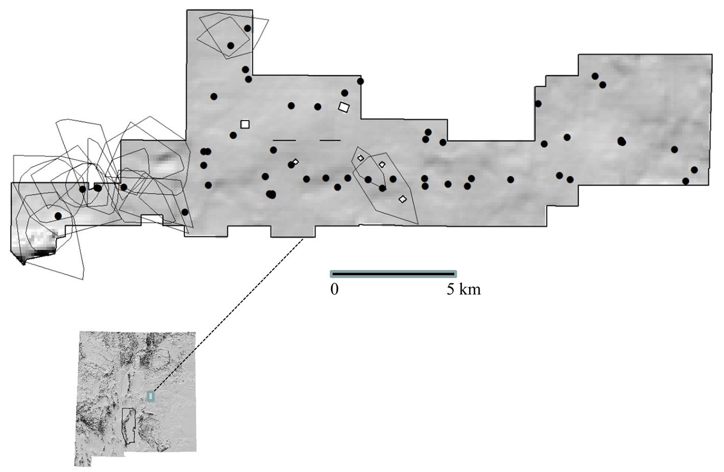
Figure 1. Topographic hillshade showing locations of annual home ranges of adult female mule deer (Bender et al., 2013), and locations of permanent water sources on the Corona Range and Livestock Research Center (CRLRC), east-central New
Mexico, USA.
We compared movement distances (km from continuous-time movement models [ctmms]; m between successive subdaily locations) between seasons using PROC GLIMMIX in SAS 9.4 (SAS, 1988), using individual deer as a random effect. We also compared mean daily and subdaily movements between successive seasons for individual deer for which we had both winter and subsequent spring-autumn data, or spring-autumn and subsequent winter data, available. We determined mean seasonal differences in movement distances for each successive time period for each individual, and used bootstrapping with N = 1,000 iterations to determine the probability that mean movement distances differed seasonally for this subset of data (see Efron & Tibshirani, 1993).
Additionally, because lactating females enter winter in poorer condition than do dry females and condition subsequently converges between the 2 classes over winter (including on the CRLRC; Bender & Hoenes, 2017), lactation status might affect desire or need to forage and thus movements of deer. However, because deer condition was very low on CRLRC during our study (i.e., lactating females were able to accrue only ≤ 5.7% percent body fat annually at the annual peak in late autumn; Bender et al., 2011, 2013), our GPS/VHF collared sample contained ≤ 2 lactating females each year, and thus we were unable to meaningfully include lactation status in our analyses. Consequently, we explored any potential effect of lactation status on movements by determining the percentile movement distances of lactating females relative to the frequency distribution of dry female movement distances to determine whether lactating females were closer to the mean or extremes of the range of dry females.
Lastly, because our GPS collared sample comprised a limited proportion of the overall radio-collared sample, we compared annual, spring-autumn, and winter home range sizes (Bender et al. 2013; N = 18-27 collared females annually) to see whether movements of our GPS sample were representative of radio-collared deer in general, comprised of N = 18-27 VHF-only collared adult females for each season (Bender et al., 2011, 2013). For this we compared annual and seasonal home range sizes of the 2 classes (GPS/VHF and VHF-only) using PROC GLM (SAS, 1988), specifically testing the year × class interaction. We visually located all deer (i.e., both GPS/VHF and VHF-only) via ground tracking of VHF signals a minimum of once per week with additional location emphasis on spring-autumn locations, and mapped locations using the Geographic Information System software package ArcGIS 10.0 (Environmental Systems Research Institute, Redlands, California, USA) (Bender et al., 2011, 2013). We constructed 95% minimum convex polygon (MCP) annual and seasonal home ranges after determining the minimum number of locations to adequately estimate seasonal home range size by plotting size as a function of number of locations (Bender et al. 2013; Kie et al. 1996). For this comparison we used only VHF visual locations of GPS/VHF collared deer so that both GPS/VHF and VHF-only samples were comprised of comparable data.
Results
We collected GPS movement data for 37 seasonal ranges (Table 2), winter 2005-6 through winter 2007-8, from 6-10 GPS/VHF collared adult females annually (mean = 336 and 472 locations per deer for winter and spring-autumn ranges, respectively). For all deer, the OUF-anisotropic movement model provided the best fit (i.e., AICc < 2 vs. all other models) of deer movements. The OUF-anisotropic movement model is the most general of ctmms, and includes a home range, correlated positions, correlated velocities, and movements varying by direction (Calabrese et al., 2021; Fleming et al., 2014).
Table 2
Mean distance moved by adult female mule deer during winter (Dec.-Feb.) and spring-autumn (Mar.-Nov.) seasons as estimated by continuous-time movement modeling (daily) and subdaily straight line movements between successive 4 h locations (subdaily) on the Corona Range and Livestock Research Center, east-central New Mexico, 2005-2007.
| Daily (km) | Subdaily (m) | |||||
| Season | Distance | SE | N | Distance | SE | N |
| Winter | 2.90 | 0.24 | 24 | 302 | 19 | 24 |
| Spring-Autumn | 4.34 | 0.43 | 13 | 409 | 44 | 13 |
Deer moved less during the winter (Table 2) for both daily ctmms (F1,20 = 6.0; p = 0.024) and minimum subdaily straight-line distances (F1,20 = 4.8; p = 0.041); in both cases the magnitude of differences varied among individual deer (t15 < -2.72; p < 0.016). Similarly, for deer for which movement data for successive seasons were available, movements between successive seasons were always less during the winter season (p (winter < spring-autumn) = 1.000) than the following or preceding spring-autumn season (Table 3).
Additionally, movement distances of lactating females (mean = 42nd percentile; range = 34-55th percentile) were always closer to the average than the extremes of the frequency distribution of movement distances of dry females for each period. Last, neither annual, spring-autumn, or winter home MCP range sizes (N = 7-16 per period) differed between GPS/VHF and VHF-only collared deer (F5,39 ≤ 0.94; p ≥ 0.599).
Discussion
Despite much less snow and warmer winter temperatures, mule deer females moved less during winter regardless of movement period (i.e., daily, subdaily), supporting the maintenance of this energy conservation behavior in mule deer in the arid Southwest (Verme & Ullrey, 1984). Because deep snow cover and very cold temperatures are typically lacking in the arid Southwest, our results further support low forage quality and availability being the primary drivers of this behavior in deer (Verme & Ullrey, 1984; see below). This latter was reflected by the poor nutritional condition of lactating adult females in the study area (i.e., <5.7% body fat annually at the annual peak in late autumn; Bender et al., 2011, 2013), and in the arid Southwest in general (Bender et al., 2007, 2011, 2012; Bender, 2020), as well as the significant losses in condition seen over winter (Bender & Hoenes, 2017; Hoenes, 2008), despite mule deer likely requiring lower quality forage than white-tailed deer (O. virginianus) (Staudenmaier et al., 2022).
While lack of deep snow cover may result in relative forage availability being less impacted during winter in the arid Southwest, senesced forages are still of very low quality, similar to northern environments (Kemp, 1983; Krausman et al., 1990; McKinney, 2003). Low forage quality in winter was reflected in the condition dynamics of deer on the CRLRC; for example, dry females lost on average 32% of body fat reserves and 38% of rump body condition score over winter (L. Bender, unpublished data), even though their condition in late autumn-early winter was already low relative to other southwestern populations (Bender et al., 2007, 2011, 2012). The nutritional condition of deer is driven primarily by forage quality (Bender, 2020; National Research Council, 2007; Tollefson et al., 2010; Verme & Ullrey, 1984; Wakeling & Bender, 2003), illustrating that deer in the arid Southwest face similar constraints in terms of limited nutrient gains from forage intake as do deer in northern environments during winter.
Table 3
Mean movement distances (x) and mean differences (D) in mean distance moved daily as predicted by continuous-time movement modeling (daily) and subdaily straight line movements between successive 4 h locations (subdaily) of adult female mule deer for which movement data for successive seasons were available between winter (Dec.-Feb.) and spring-autumn (Mar.-Nov.) on the Corona Range and Livestock Research Center, east-central New Mexico, 2005-2007. p = Probability that seasonal differences differ from 0; N = number of seasonal comparisons.
| Period | x Summer | x Winter | D | 90% CI | p | N |
| Subdaily | 400.2 | 309.6 | -90.6 m | -123- -63 | 1.000 | 20 |
| Daily | 4.21 | 3.16 | -1.05 km | -1.53- -0.63 | 1.000 | 20 |
Deer in northern environments do face additional energetic challenges associated with persistent snow cover, which can limit forage availability (by making location and acquisition of food more difficult; Hovey & Harstad, 1992), diet quality (due to reduced forage quality and availability; McKinney, 2003; Osborn & Jenks, 1998), and increase loss of endogenous reserves (because of increased costs of moving through snow; Bunnell et al., 1990; Mattfeld, 1973). However, while deer in the arid Southwest are less influenced by snow-depth related challenges, northern deer do not face the lack of free water experienced by most deer populations in arid environments because of persistent snow cover in northern environments. Lack of water can present an energetic cost to deer in the arid Southwest, as mule deer may increase movement distances to access water (Heffelfinger, 2006), and winter is much drier than spring-autumn in Chihuahuan desert and short-grass prairie habitats of the arid Southwest (e.g., 87% of precipitation occurs during spring-autumn on the CRLRC).
Because of permanent water developments, water was comparably available seasonally on the CRLRC; water developments were accessible from all deer home ranges, so mule deer did not need to alter their movements in response to seasonal changes in availability of water. Hence, need or preference for free water likely had a negligible effect on deer movements on the CRLRC, unless presence of temporary sources (ephemeral pools, etc.) during the summer monsoon reduce deer movements during spring-autumn because of increased availability. Thus, despite water being effectively controlled in our study, deer still showed less movements during winter. This again supports decreased movements during winter being most influenced by the lack of energetic benefit from seeking and foraging on low quality senesced forage.
Cold temperatures are often thought to influence the winter conservation strategy, despite demonstrated lack of benefit of thermal cover in winter to deer (Cook et al., 1998; Freddy, 1984), the pronounced effect of solar radiation on warming deer (Cook et al., 1998; Parker & Gillingham, 1990; Parker & Robbins, 1984), and deer movements and tolerance of exposure to cold (including bedding in the open) except during the most extreme conditions when high quality forage is available (Moen, 1968; Verme & Ullrey, 1984). Mule deer possess a low thermal critical zone (ca. -20 oC) and show greater tolerance of cold than do white-tailed deer, including a lower metabolic rate response to decreasing temperatures (Mautz et al., 1985; Parker & Robbins, 1984). Hence, they are less affected by even extreme cold, which is seldom the case in the arid Southwest where mean low temperatures seldom approach their lower thermal tolerance (Table 1). Conversely, the upper thermal critical level of mule deer in winter pelage (5 ºC; Mautz et al., 1985) is lower than average high temperatures during winter on our study area (6.7-8.9 ºC; Table 1) and much of the arid Southwest. This would require active metabolic activity or behaviors (e.g., panting, etc.) by mule deer to cool themselves, or possibly limiting movements and bedding under shade (although the energetic benefits of the latter are questionable; Cook et al., 1998). Consequently, if temperature affected movements during the winter in our study area, deer would be more likely to decrease movements because of heat stress, not cold stress.
Lastly, while at least one behavioral aspect of the winter energy conservation strategy is seen in mule deer in the arid Southwest, to what degree other adaptations are conserved is unknown. Mule deer in the arid Southwest do develop a highly insulative pelage in winter (Heffelfinger, 2006), but the extent that they may decrease metabolic rate or regulate vascular circulation to the extremities (or need to, in light of the more moderate temperatures) is unknown. Additionally, while lactating females showed a tendency to move less relative to dry females on the CRLRC, whether this is typical is unknown because of our small sample of lactating females. However, given that most females on CRLRC were in poorer condition than females elsewhere in the arid Southwest (Bender et al., 2007, 2011, 2012; Bender & Hoenes, 2017), if very low condition (such as results from lactation) increases movements during winter, this increase would likely have been seen in all CRLRC females regardless of lactation status. Moreover, GPS/VHF and VHF-only collared females showed similar movements (as indexed by home range sizes) seasonally and annually on CRLRC, indicating that movements of GPS/VHF collared females reflected females in general. Although small sample sizes (3-4) precluded including lactation status as an interactive term in the contrast of GPS/VHF and VHF-only collared females, for all females lactation status had no effect on annual or seasonal home range sizes (p ≥ 0.599).
Acknowledgments
Support for this project was provided by the U.S. Forest Service-Rocky Mountain Research Station and the New Mexico State University Cooperative Extension Service and Agricultural Experimental Station. All activities were in accordance with NMSU IACUC Permit No. 2005-023. E.J.T.-R. was supported by a postdoctoral fellowship from Consejo Nacional de Humanidades, Ciencias y Tecnologías (Conahcyt-Mexico).
References
Alldredge, A. W., Lipscomb, J.F., & Whicker, F.W. (1974). Forage intake rates of mule deer estimated with fallout
cesium-137. The Journal of Wildlife Management, 38, 508–516. https://doi.org/10.2307/3800882
Bartmann, R. M., & Bowden, D. C. (1984). Predicting mule deer mortality from weather data in Colorado. Wildlife Society Bulletin, 12, 246–248. https://doi.org/10.1002/jwmg.956
Bender, L. C. (2020). Elk, deer, and pinyon-juniper: needs, what works, and what doesn’t. In K. Malcolm, B. Dykstra, K. Johnson, D. Lightfoot, E. Muldavin, & M. Ramsey (Compilers), Symposium proceedings on piñon-juniper habitats: status and management for wildlife – 2016. Proceedings RMRS-P-77. Fort Collins, Colorado: U.S. Forest Service, Rocky Mountain Research Station.
Bender, L. C., & Hoenes, B. D. (2017). Costs of lactation to body condition and future reproduction of free-ranging mule deer Odocoileus hemionus (Cervidae). Mammalia, 81, 329–338. https://doi.org/10.1515/mammalia-2015-0143
Bender, L. C., Lomas, L. A., & Browning, J. (2007). Condition, survival, and cause-specific mortality of mule deer in northcentral New Mexico. Journal of Wildlife Management, 71, 1118–1124. https://doi.org/10.2193/2006-226
Bender, L. C., Boren, J. C., Halbritter, H., & Cox, S. (2011). Condition, survival, and productivity of mule deer in semiarid grassland-woodland in east-central New Mexico. Human-Wildlife Interactions, 5, 276–286. https://doi.org/10.26077/60n0-ks48
Bender, L. C., Hoenes, B. D., & Rodden, C. L. (2012). Factors influencing survival of desert mule deer in the greater San Andres Mountains, New Mexico. Human-Wildlife Interactions, 6, 245–260. https://doi.org/10.26077/h5bg-1829
Bender, L. C., Boren, J. C., Halbritter, H., & Cox, S. (2013). Effects of site characteristics, pinyon-juniper control, and precipitation on habitat quality for mule deer on the Corona Range and Livestock Research Center. Human-Wildlife Interactions, 7, 47–59. https://digitalcommons.usu.edu/hwi/vol7/iss1/5
Bunnell, F. L., Hovey, F. W., McNay, R. S., & Parker, K. L. (1990). Forest cover, snow conditions, and black-tailed deer sinking depths. Canadian Journal of Zoology, 68, 2403–2408. https://doi.org/10.1139/z90-333
Calabrese, J. M., Fleming, C. H., & Gurarie, E. (2016). ctmm: an R package for analyzing animal relocation data as a continuous-time stochastic process. Methods in Ecology and Evolution, 7, 1124–1132. https://doi.org/10.1111/2041-210X.12559
Calabrese, J. M., Fleming, C. H., Noonan, M. J., & Dong, X. (2021). ctmmweb: a graphical user interface for autocorrelation-informed home range estimation. Wildlife Society Bulletin, 45, 162–169. https://doi.org/10.1002/wsb.1154
Cook, J. G., Irwin, L. L., Bryant, L. D., Riggs, R. A., & Thomas, J. W. (1998). Relations of forest cover and condition of elk: a test of the thermal cover hypothesis in summer and winter. Wildlife Monographs, 141, 1–61.
Efron, B., & Tibshirani, R. J. (1993). An introduction to the bootstrap. New York: Chapman & Hall.
Fleming, C. H., Fagan, W. F., Mueller, T., Olson, K. A., Leimgruber, P., & Calabrese, J. M. (2014). From fine-scale foraging to home ranges: a semivariance approach to identifying movement modes across spatiotemporal scales. American Naturalist, 183, E154–E167. http://doi.org/10.1086/675504
Fleming, C. H., Fagan, W. F., Mueller, T., Olson, K. A., Leimgruber, P., & Calabrese, J. M. (2016). Estimating where and how animals travel: an optimal framework for path reconstruction from autocorrelated tracking data. Ecology, 97, 576–582. https://doi.org/10.1890/15-1607.1
Freddy, D. J. (1984). Quantifying capacity of winter ranges to support deer – evaluation of thermal cover used by deer. Denver, CO: Wildlife Research Report, Colorado Division of Wildlife, USA.
Heffelfinger, J. (2006). Deer of the Southwest: a complete guide to the natural history, biology, and management of Southwestern mule deer and white-tailed deer. Texas A&M University, College Station, Texas.
Hoenes, B. D. (2008). Identification of factors limiting desert mule deer populations in the greater San Andres Mountains of southcentral New Mexico (Thesis). New Mexico State University, Las Cruces.
Hovey, F. W., & Harestad, A. S. (1992). Estimating effects of snow on shrub availability for black-tailed deer in southwestern British Columbia. Wildlife Society Bulletin, 20, 308–313.
Jacobsen, N. K. (1980). Differences of thermal properties of white-tailed deer pelage between seasons and body regions. Journal of Thermal Biology, 5, 151–158. https://doi.org/10.1016/0306-4565(80)90014-5
Kemp, P. R. (1983). Phenological patterns of Chihuahuan desert plants in relation to the timing of water availability. Journal of Ecology, 71, 427–436.
Kie, J. G., Baldwin, J. A., & Evans, C. J. (1996). CALHOME: a program for estimating animal home ranges. Wildlife Society Bulletin, 24, 342–344.
Krausman, P. R., Ordway, L. L., Whiting, F. M., & Brown, W. H. (1990). Nutritional composition of desert mule deer forage in the Picacho Mountains, Arizona. Desert Plants, 10, 32–34.
Marchinton, R. L., & Hirth, D. H. (1984). Behavior. In L. K. Halls (Ed.), White-tailed deer ecology and management. Pennsylvania: Stackpole Books.
Marshal, J. P., Krausman, P. R., & Bleich, V. C. (2008). Body condition of mule deer in the Sonoran Desert is related to rainfall. Southwestern Naturalist, 53, 311–318. https://doi.org/10.1894/CJ-143.1
Mattfeld, G. F. (1973). The effect of snow on the energy expenditure of walking white-tailed deer. In Transactions of the 30th Northeast Fish and Wildlife Conference, Dover, Vermont, Spring, April 1973.
Mautz, W. W., Pekins, P. J., & Warren, J. A. (1985). Cold temperature effects on metabolic rates of white-tailed, mule, and black-tailed deer in winter coat. In P. F. Fennessy, & K. R. Orew (Eds.), The biology of deer. Royal Society of New Zealand Bulletin, 22, 453–457.
McKinney, T. (2003). Precipitation, weather, and mule deer. In J. C. Jr. deVos, M. R. Conover, & N. E. Headrick (Eds.), Mule deer conservation. Issues and management strategies. Logan, Utah: Jack H. Berryman Press.
Moen, A. N. (1968). Energy exchange of white-tailed deer, western Minnesota. Ecology, 49, 676–682. https://doi.org/10.2307/1935531
National Research Council (US). (2007). Committee on Nutrient Requirements of Small Ruminants. Nutrient requirements of small ruminants: sheep, goats, cervids, and New World camelids. Washington D.C.: National Academy Press.
Osborn, R. G., & Jenks, J. A. (1998). Assessing dietary quality of white-tailed deer using fecal indices: effects of supplemental feeding and area. Journal of Mammalogy, 79, 437–447. https://doi.org/10.2307/1382974
Parker, K. L., & Robbins, C. T. (1984). Thermoregulation in mule deer and elk. Canadian Journal of Zoology, 62, 1409–1422. https://doi.org/10.1139/z84-202
Parker, K. L., & Gillingham, M. P. (1990). Estimates of critical thermal environments for mule deer. Journal of Range Management, 43, 73–81. http://doi.org/10.2307/3899126
Robinette, W. L., Jones, D. A., Rogers, G., & Gashwiler, J. S. (1957). Notes on tooth development and wear for Rocky Mountain mule deer. Journal of Wildlife Management, 21, 134–153. https://doi.org/10.2307/3797579
SAS. (1988). SAS/STAT user’s guide. SAS Institute Incorporated, Cary, North Carolina.
Short, H. L. (1981). Nutrition and metabolism. In O. C. Wallmo, R. E. McCabe, & L. R. Jahn (Eds.), Mule and black-tailed deer of North America. Lincoln: University of Nebraska Press.
Silver, H., Holter, J. B., Colovox, N. F., & Hayes, H. H. (1971). Effect of falling temperature on heat production in fasting white-tailed deer. Journal of Wildlife Management, 35, 37–46.
Staudenmaier, A. R., Shipley, L. A., Camp, M. J., Forbey, J. S., Hagerman, A. E., Brandt, A. E. et al. (2022). Mule deer do more with less: comparing their nutritional requirements and tolerances with white-tailed deer. Journal of Mammalogy, 103, 178–195. https://doi.org/10.1093/jmammal/gyab116
Tollefson, T. N., Shipley, L. A., Myers, W. L., Keisler, D. H., & Dasgupta, N. (2010). Influence of summer-autumn nutrition on body condition and reproduction in lactating mule deer. Journal of Wildlife Management, 74, 974–986. https://doi.org/10.2193/2008-529
Verme, L. J., & Ullrey, D. E. (1984). Physiology and nutrition. In L. K. Halls (Ed.), White-tailed deer: Ecology and management. Harrisburg, Pennsylvania: Stackpole Books.
Wakeling, B. F., & Bender, L. C. (2003). Influence of nutrition on mule deer biology and ecology. In J. C. Jr. deVos, M. R. Conover, & N. E. Headrick (Eds.), Mule deer conservation. Issues and management strategies. Logan, Utah: Jack H. Berryman Press.

Impacts of disturbance on ant (Hymenoptera:Formicidae) food preferences and dominance in a Mexican temperate forest.
Meghan I. Zolá-Rodríguez a, Mariana Cuautle b, *, Marco Daniel Rodríguez-Flores c, Citlalli Castillo-Guevara b
a Akumal Monkey Sanctuary & Rescued Animals, Camino a Uxuxubi s/n Predio Santa Pilar Lote 16, 77776 Akumal, Quintana Roo, Mexico
b Universidad Autónoma de Tlaxcala, Centro de Investigación en Ciencias Biológicas, Km 10.5 Carretera Tlaxcala-San Martín Texmelucan, 90120 San Felipe Ixtacuixtla, Tlaxcala, Mexico
c Blue Marlin Conservation (Conservation Diver), Sunset Beach Gili Air, Gili Indah, Pemenang, North Lombok Regency, West Nusa Tenggara 83355, Indonesia
*Corresponding author: mcuautle2004@gmail.com (M. Cuautle)
Received: 26 June 2024; accepted: 27 August 2024
Abstract
This study examines the impact of disturbance on the food preferences and dominance of an ant community in a temperate ecosystem in Mexico. The study focused on 2 types of vegetation: native oak forest and induced grassland (disturbed vegetation). Observations were conducted to record the food elements carried by ants to their nests. These data were analyzed using x2 tests. Tuna and honey baits were placed near the nests to record the presence of ants in 5-minute periods. We used a binomial model to determine whether the probability of finding an ant foraging at the baits was affected by vegetation type, bait type, and/or ant species. Additional baits were used to determine the ant dominance indices. T-tests and ANOVAs were used to compare dominance indices between vegetation types, baits, and ant species. No significant differences were observed in food preferences between vegetations. However, some species showed a preference for honey (i.e., carbohydrates), which could be limited in ground-level environments. Ants showed a submissive behavior in both vegetation types. This research shows that ants could optimize their nutrient intake, enabling them to survive efficiently even when facing disturbances, instead of increasing dominance.
Keywords: Ant nest; Dominance index; Feeding habits; Compensation hypothesis; Carbohydrates; Proteins
© 2024 Universidad Nacional Autónoma de México, Instituto de Biología. Este es un artículo Open Access bajo la licencia CC BY-NC-ND
(http://creativecommons.org/licenses/by-nc-nd/4.0/).
Impacto del disturbio en las preferencias alimentarias y dominancia de las hormigas (Hymenoptera: Formicidae) en un bosque templado de México
Resumen
Este estudio examina el impacto del disturbio en las preferencias alimentarias y dominancia de una comunidad de hormigas en un ecosistema templado en México, en bosque de encino nativo y pastizal inducido (vegetación perturbada). Se registraron los alimentos transportados por las hormigas a sus nidos. Estos datos fueron analizados utilizando pruebas de x2. Se colocaron cebos de atún y miel cerca de los nidos para registrar la presencia de hormigas. Utilizamos un modelo binomial para determinar si la probabilidad de encontrar una hormiga en los cebos se veía afectada por la vegetación, cebo o especie de hormiga. Los índices de dominancia se determinaron usando cebos. Se emplearon pruebas t y Anova para comparar los índices de dominancia entre tipos de vegetación, cebos y especies de hormigas. No hubo diferencias significativas en las preferencias alimentarias entre tipos de vegetación, pero algunas especies mostraron una preferencia por la miel (carbohidratos), que podría ser un recurso limitado a nivel del suelo. Las hormigas mostraron un comportamiento sumiso en ambos tipos de vegetación. Esta investigación muestra que las hormigas podrían optimizar su ingesta de nutrientes, permitiéndoles sobrevivir bajo condiciones de disturbio, en lugar de aumentar su dominancia.
Palabras clave:Nidos de hormigas; Índice de dominancia; Hábitos alimenticios; Hipótesis de compensación; Carbohidratos; Proteínas
Introduction
Land use change stands as one of the primary factors contributing to global change and its adverse effects on biodiversity (Ellis et al., 2010; Foley et al., 2005; Sala et al., 2000). Land use change has reduced biodiversity through the loss, modification, and fragmentation of habitats; degradation of soil and water; and overexploitation of native species (Foley et al., 2005), and its effects depend strongly on the type, severity, frequency and timing of disturbance (Foley et al., 2005; White & Jentsch, 2001). Ants are one of the most dominant insects both ecologically and numerically (Rico-Gray & Oliveira, 2007; Schultheiss et al., 2022; Toro et al., 2012) that participate in different ecological processes —e.g., nutrient recycling, soil formation, decomposition, seed dispersion (Toro et al., 2012). Ants are model organisms to study the effect of disturbance because they respond to environmental change (Agosti et al., 2000; Andersen, 2000). It is often observed that disturbances favor behaviorally dominant ants, including invasive species. Vonshak and Gordon (2015), observed that native ant richness was highest in natural habitats, and alien species richness was highest in urban habitats, along an urban-rural gradient in the San Francisco Bay area. Nevertheless, the specific effect will depend on factors like the type of disturbance, including fires, floodings, or even treefall gaps (Cerdá et al., 2013). Hoffman and Andersen (2003) studied the response of ant functional groups to disturbance finding that the dominant Dolichoderinae and “hot climate specialists” tend to be favoured by low levels of disturbance. The opportunist and generalized Myrmicinae have wide habitat tolerances but are sensitive to competitive interactions, while “cryptic species” and “specialist predators” are highly sensitive to disturbance.
Feeding habits and foraging strategies represent vital life history traits among ants, playing a significant role in their ecological dynamics. These traits are contingent upon the availability of resources within their respective habitats (Andersen, 2000; Davidson, 2005), and the ensuing competition for those resources (Arnan et al., 2012). The feeding habits of ants play a pivotal role in determining their ecological function within the ecosystem (Spotti et al., 2015). However, despite their significance, the food habits and preferences of ants remain relatively understudied and represent one of the least understood aspects of their biology (Houdria et al., 2015).
The effects of disturbance (e.g., land use change) on ant feeding habits (especially foraging strategies) have not been studied in depth (Castillo-Guevara et al., 2019; Hernández-Flores et al., 2016; Radnan et al., 2018), and the way ants respond to habitat complexity can provide clues as to how ants could respond to disturbance. When the external disturbing factors are of high intensity (natural-fires or anthropogenic-deforestation), the disturbances can initiate a directional regression manifested as gradual or rapid simplification of the horizontal and vertical structure of a community, leading to the replacement of complex communities by a simpler one (Łaska, 2001). The level of habitat complexity can influence ant foraging patterns. For instance, higher complexity may decrease interspecific interactions and ant recruitment or minimize the trade-off between resource discovery and dominance (Parr & Gibb, 2012).
Examining the effect of soil surface complexity on food exploitation in the context of change from grassland to shrubland in Australia, Radnan et al. (2018) discovered that substrate complexity (wood debris, leaf litter, or no substrate) influenced the discovery time, ant size, and monopolization index of tuna and honey baits within testing arenas. However, at a larger scale of vegetation type, the effect was not observed. Similarly, Castillo-Guevara et al. (2019) found that the dominance level was similar in natural oak vegetation in comparison to an agricultural area in a temperate community; however, ant foraging strategies differed between the 2 communities.
Competition has been regarded as the primary factor influencing the structure of ant communities (Cerdá et al., 2013). Through the use of aggressive strategies, ants exert influence on the spatial distribution, abundance, and behavior of other ants. These strategies encompass a range of tactics, including the deployment of repellent chemicals and the establishment of territories (Cerdá et al., 2013). Moreover, ants can establish interspecific dominance hierarchies primarily based on variations in food collection behavior and aggressiveness. While there are various proposals for categorizing such hierarchies, the classification proposed by Vepsäläinen and Pisarski (1982) and Savolainen et al. (1989), as described by Cerdá et al. (2013), is considered the most well-defined hierarchical system from an ecological perspective. This classification system is founded on the aggressive behavior of ants and its impact on other ant species, and includes 3 categories: the dominant, subdominant and subordinate category. Dominant species exhibit highly aggressive behavior, exhibit numerical predominance over other species, fiercely defend their territories, and establish mutual exclusivity within their ecological communities. Subdominant species, while not actively defending territories, display a remarkable propensity for aggressively safeguarding their food resources (Cerdá et al., 2013). Lastly, subordinate species, characterized by small colonies devoid of recruitment systems, employ strategies to avoid physical confrontations with other colonies and species. Nonetheless, they exhibit a strong commitment to defending their nests against potential threats (Cerdá et al., 2013). Different foraging strategies, such as the subordinate species’ ability to discover resources before dominant species (dominance-discovery trade-off, Fellers, 1987) or their capacity to forage across a broader temperature range compared to dominant species —dominance-thermal tolerance trade-off (Fellers, 1989), can contribute to the coexistence of ants within a community.
The present study focuses on the analysis of ant feeding habits and dominance hierarchy in response to land use change within a temperate ecosystem located in central Mexico. A habitat with the native oak forest vegetation (complex habitat), was compared to a nearby area where the land use had been altered to induced grassland (simplified habitat). The study hypothesized: i) it is expected that in the oak forest, food items transported to the nest will be more varied than in the induced grassland. This variation at the species level is also anticipated due to the change in land use. The conversion from a complex habitat (oak forest) to a simplified habitat (induced grassland) will likely provide fewer resources variety for the ants; ii) it is expected that as a result of the disturbance in the induced grassland, ants will be more generalized in low heterogeneous habitats due to the dominance of generalist ant species. Additionally, the arrival times at the baits will be shorter due to the absence of leaf litter; iii) a lower dominance index is expected in the induced grassland than in the oak forest, due to the presence of subdominant species and the modification of the dominance hierarchy system by the land use change.
Materials and methods
The study was conducted within “Flor del Bosque” State Park, located in the municipality of Amozoc de Mota, in the state of Puebla. The coordinates of this protected reserve are 19°00’00”-19°01’50” N, 98°20’35”-98°20’53” W. The State Park encompasses an area of 664.03 hectares, characterized by altitudes ranging from 2,225 to 2,400 m asl. The annual average temperature in this region fluctuates between 14 °C and 16 °C, with the majority of rainfall occurring during the summer months, contributing to an average annual precipitation of 750 to 950 mm. It is important to note that the park experiences a distinct dry season lasting approximately 6 months, from November to April, as reported by Costes et al. (2006). The native vegetation of the reserve primarily consists of oak forest [Quercus castanea (Née), Q. laurina (Bonpl.), Q. laeta (Liebm.) (Fagaceae)]. However, human disturbances have led to the presence of induced grassland areas and, to a lesser extent, eucalyptus plantations [Eucalyptus spp. L´Hér) (Myrtaceae)] within the park, as documented by Costes et al. (2006). Given that the disturbed vegetation within the reserve primarily consisted of induced grassland, our research aimed to establish a meaningful comparison between native and altered vegetation.
Ant communities were surveyed once a month during specific periods (April, August and October 2015, and January to March 2016). The survey methodology involved the establishment of 6 transect plots (400 m × 20 m), with 3 plots located in the oak forest and 3 in the induced grassland. The spatial distribution of these transects can be observed in Figure 1. To locate ant nests, the transects were traversed, and various substrates such as leaf litter, stones, trunks, and branches were lifted and examined. Additionally, a total of 5 tuna baits and 5 honey baits were placed along the transects at 10 m intervals to attract ants and to follow them to locate their nest. The nests found during the survey were georeferenced for accurate spatial documentation. A 5-minute observation period was designated for each nest, wherein all food items transported by the ants to their nests were recorded. These observations were conducted between 9:00 a.m. and 3:00 p.m. on the sampling days. Each recorded item was subsequently categorized into one of the following groups: 1) plant elements, encompassing any component of plants except for seeds, 2) seeds, and 3) arthropods. After each observation period, 2 bait samples, enclosed within Petri dishes, were positioned in close proximity to the nests (approximately 10 cm), maintaining a distance of approximately 5 centimeters from each other. Various studies exploring the feeding habits, preferences, and foraging strategies of ants have employed diverse bait types. Typically, these baits consist of carbohydrates such as honey and other sources representing proteins such as tuna (Houdria et al., 2015; Lynch et al., 1980; Spotti et al., 2015; Trigos-Peral et al., 2016). The bait materials employed in the study consisted of honey and tuna, which were consistently provided in a standardized amount of one tablespoon, equivalent to approximately 5 grams. To quantify the number of individual ants on each type of food resource, we placed baits and observed them for 5 min. Ants responded very quickly to the baits; therefore, the observation time was limited to 5 min. Within this duration, the number of individuals was recorded for each bait type. After the observation periods, 1 to 3 ants were collected from each nest using a vacuum cleaner or tweezers and then preserved in Eppendorf tubes containing 70% ethanol. In the laboratory, the ants were separated, mounted, and identified to the genus level using the key by Mackay and Mackay (1989). In certain instances, the species identification was feasible by comparing the collected specimens with those present in the Entomological Collection of the Universidad de las Américas Puebla (UDLAP).
To analyze the food preferences of the ant community, we considered 3 factors. First, we determined whether the number of foragers carrying plants, seeds, or arthropods to the nest differed between the whole ant communities of each vegetation type or among ant species. We used the appropriate contingency tables and chi-square tests for such comparisons. Second, we determined whether the presence of foragers at each bait during each minute of the 5-minute period was influenced by vegetation type, bait type (honey or tuna), ant species or interactions among these factors. We used a binomial model to evaluate this response variable, with “ant presence” coded as 1 and “absence” as 0. To select the most relevant explanatory variables, we employed a stepwise forward approach. We began with the simplest model and successively added each response variable. The significance of adding each variable was assessed using an x2 test, comparing the previous model with the new model. If a variable was found to be statistically significant, it was retained in the model. Otherwise, it was removed, and we proceeded with the next explanatory variable. This stepwise procedure allowed us to build the final model with the most significant factors explaining the presence of foragers at each bait. No overdispersion was detected in the selected model. Post-hoc analyses were conducted when significant differences were detected. The statistical analysis of data was performed using R software (R Core Team, 2022).
We evaluated the dominance hierarchy of the ants in each vegetation type (oak forest and induced grassland), ant species, and bait types using the same transects as for the detection of the nests (Fig. 1), during October 2015 and January, February and March (2016). At each transect, 9 sampling points were established on the ground, spaced 10 m apart. Each sampling point consisted of a pair of Petri dishes with baits: one with honey and one with tuna, placed less than 5 cm apart. This resulted in a total of 540 baits (5 replicates × 6 transects × 9 sampling points × 2 baits; 2 samplings in February). These types of baits have been widely used for ant dominance hierarchy studies (Dáttilo et al., 2014; Parr & Gibb, 2012; Trigos-Peral et al., 2016).
For the first 3 sets of bait, we recorded the arrival times of the ants during a one-hour observation period. Most of the ant species were identified in the field. For the ants that were not identified, a few individuals (2 to 3 specimens) were collected. In the case of the remaining 6 sets of bait, they were filled with water. Ants that fell onto the Petri dish after 2 h were collected. The presence of water did not deter the ants from visiting, but it allowed us to determine which ants had been attracted to the baits. The baits were placed and retrieved from different transects in the field between 9:00 a.m. and 5:00 p.m. The order of the transects was changed on different sampling days to mitigate the potential impact of the time of day. Ant specimens collected from the baits were preserved in 70% ethanol and transported to the laboratory for further identification.

Figure 1. Localization of the transects used in the study zone (mapped by Luna F.).
We chose numerical dominance to assess the dominance hierarchy of the ants —i.e., ordering of ant species based on their numerical or behavioral dominance by vegetation types (Andersen, 1992; Cerdá et al., 1997; Stuble et al., 2017), ant species and bait type. As numerical and behavioral dominance are highly correlated, this method has been well-established and documented in the ant literature (Dáttilo et al., 2014; Dejean & Corbara, 2003; Parr, 2008; Parr & Gibb, 2012; Santini et al., 2007). This method indicates which species are consistently present at the baits, and which ones dominate the baits numerically and thus monopolize them (Parr, 2008). We represented numerical dominance using the numerical dominance index (DI) for each morphospecies calculated by the formula: DI = (Di)/(Di + Si), where, Di is the number of baits monopolized by the species of ant i, and Si is the number of baits that the species of ant i used but did not monopolize. Baits were considered to be monopolized when more than 5 individuals (workers and/or soldiers) of the same morphospecies were using the resource without the presence of other morphospecies. This measure (more than 5 individuals) takes into consideration that in temperate climates, ants are less abundant, and recruitment is considered weaker than in tropical environments where the index has been widely more (Santini et al., 2007). Therefore, dominant morphospecies are those that find and monopolize a larger proportion of the food resources in a given environment. The value of the index ranges from 0 (completely submissive species) to 1 (totally dominant species) and is similar to the “monopolization index” used in other studies (Dáttilo et al., 2014; Fellers, 1987; Parr & Gibb, 2012; Santini, et al., 2007). In this study, ant species with a DI lower than 0.5 were classified as submissive.
The arrival times of the ants were compared using survival curves using the survival package of the R Software program. The one-hour and 2-hour baits were used to calculate the ID of the ant species. To compare the ID between vegetation and bait types, t-tests were performed. To compare the DI between ant species, a one-way ANOVA test was performed after applying a square root transformation to meet the normality requirements. These analyses were performed using the program STATVIEW 5.0 (Abacus Concepts Inc., 1996).
Results
Fourteen morphospecies of ants were recorded in this study belonging to 11 ant genera (Table 1). For the analysis of the results from the nests and the baits placed near them, 2 morphospecies of Pheidole were identified. However, due to the low number of records for each morphospecies across different vegetation types, Pheidole sp. 1 and Pheidole sp. 2 were combined for the analysis. In the oak forest, 2 out of 19 records corresponded to Pheidole sp. 1, and in the grassland, 4 out of 15 records corresponded to Pheidole sp. 2. Since Pheidole species often share similar feeding habits and are functionally similar (Agosti, 2000; Andersen, 2000), these 2 morphospecies were grouped to increase statistical power, and the analysis was conducted at the genus level. In contrast, another Pheidole species, Pheidole sp. 3, was recorded in the baits used to determine the DI and was analyzed independently due to its different context of occurrence. The rest of the analyses were conducted at the species level.
In the case of the nests, we found 9 morphospecies distributed among 34 nests, 19 of these were located in the oak forest and 18 in the induced grassland (Table 2). No significant differences were observed in the types of food elements those individual ants transported to their nest when comparing different vegetation types (x2 = 2.13, df = 2, p = 0.34). In the oak forest considering all ant species, there were no significant differences in the number of individuals carrying elements from different categories (x2 = 0.03, df = 1, p = 0.86) (Fig. 2). Of the genera of ants observed carrying food elements to their nests, only 2 genera were observed with a single type of food resource: Prenolepis imparis (Say) only carried arthropods and Dorymyrmex insanus (Buckley) only seeds.
Table 1
List of ant species recorded in this study in “Flor del Bosque” State Park in Puebla, Mexico.
| Formicidae/Subfamily/Ant species | |||
| Formicidae Latreille, 1809 | |||
| Dolichoderinae Forel, 1878 | |||
| Leptomyrmecini Emery, 1913 | |||
| Dorymyrmex Mayr, 1866 | |||
| Dorymyrmex insanus (Buckley, 1866) | |||
| Linepithema Mayr, 1866 | |||
| Linepithema dispertitum (Forel, 1885) | |||
| Dorylinae Leach, 1815 | |||
| Dorylini Ashmead, 1905 | |||
| Labidus Jurine, 1807 | |||
| Labidus coecus Latreille, 1802 | |||
| Formicinae Latreille, 1809 | |||
| Camponotini Forel, 1878 | |||
| Camponotus Mayr,1861 | |||
| Camponotus rubrithorax Forel, 1899 | |||
| Lasiini Ashmead, 1905 | |||
| Nylanderia Emery, 1906 | |||
| Nylanderia austroccidua Trager, 1984 | |||
| Prenolepis Mayr, 1861 | |||
| Prenolepis imparis Say, 1836 | |||
| Myrmicinae Lepeletier, 1835 | |||
| Attini Smith, 1858 | |||
| Pheidole Westwood, 1839 | |||
| Pheidole sp. 1 | |||
| Pheidole sp. 2 | |||
| Pheidole sp. 3 | |||
| Crematogastrini Forel, 1893 | |||
| Temnothorax Mayr, 1861 | |||
| Temnothorax augusti Baroni Urbani, 1978 | |||
| Pogonomyrmecini Ward, Brady, Fisher & Schultz, 2014 | |||
| Pogonomyrmex Mayr, 1868 | |||
| Pogonomyrmex barbatus (Smith, F., 1858) | |||
| Solenopsidini Forel, 1893 | |||
| Monomorium Mayr, 1855 | |||
| Monomorium ebenium Forel, 1891 | |||
| Pseudomyrmecinae, Smith, M.R., 1952 | |||
| Pseudomyrmecini Smith, 1952 | |||
| Pseudomyrmex Lund, 1831 | |||
| Pseudomyrmex pallidus Smith, F., 1855 |
Conversely, ants of the genus Pheidole spp. carried a greater quantity of plant elements compared to the other categories (x2 = 10.4, df = 2, p = 0.006); only 2 of these individuals were observed carrying arthropods, and none were recorded carrying seeds. No significant differences were found for D. insanus (x2 = 2, df = 2, p = 0.37), P. barbatus (x2 = 1.6, df = 2, p = 0.450), nor P. imparis (x2 = 4, df = 2, p = 0.135) among the 3 food categories. Only P. barbatus carried all 3 types of food (Fig. 2).
Considering all ant species, there were no significant differences in the number of individuals carrying different food elements in the induced grassland (x2 = 0.66, df = 1, p = 0.41, Fig. 2). Among the observed ant species that transported food types to their nests, P. barbatus was found to carry both plant elements and seeds. Additionally, Dorymyrmex insanus and Pheidole spp. were observed carrying food from all 3 categories (Fig. 2). Pheidole spp. (x2 = 10.33, df = 2, p = 0.006) and P. barbatus (x2 < 30.33, df = 2, p < 0.001), carried a higher number of plant elements. For D. insanus no significant differences were found in the number of elements of each type (x2 < 3.77, df = 2, p = 0.15) (Fig. 2).

Figure 2. Number of individuals of the different ant species recorded carrying any food resource to their nest. DORY: Dorymyrmex insanus, PHEI: Pheidole spp., POGO: Pogonomyrmex barbatus, PREN: Prenolepis impairs.
In the induced grassland, 5 ant species were attracted to both types of baits, and 1 species was found in the tuna baits. In the oak area, 5 ant species were observed in both types of baits, and 1 species was attracted to the honey bait (Fig. 3). The probability of presence of a forager during a given minute of the observation period depended on the vegetation type (x2= 8.73, df = 1, p = 0.03), the ant species (x2= 59.64, df = 7, p < 0.001), the interaction between the ant species and the bait (x2= 57.96, df = 8, p < 0.001), and the interaction between the vegetation type, the ant species, and the bait (x2= 26.12, df = 7, p < 0.001). The Tukey contrast test for the vegetation*species*bait interaction showed (Z > 3.83, p < 0.042) that the presence of Linepithema dispertitum (Forel) on the honey bait, in the oak forest, was more likely than the presence of Pheidole spp. on either the tuna or honey bait in the oak forest, Pheidole spp. on the honey bait in the induced grassland, and P. impairs on the honey bait in the oak forest (Fig. 3). The probability of Camponothus rubrithorax (Forel) being present on the honey bait in the induced grassland, was greater than that of D. insanus in either the tuna or honey bait in the induced grassland, Pheidole spp. on either the tuna or honey bait in the oak forest, as well as its presence in the honey bait in the induced grassland and P. imparis in the honey bait in the oak forest (Fig. 3). The probability that P. barbatus was present on the honey bait in the induced grassland, was greater than the presence of Pheidole spp. in either the tuna or honey bait and P. imparis in the honey bait in the oak forest (Fig. 3). Finally, the presence of Pheidole spp. on the tuna bait was more likely than its presence on the honey bait in the induced grassland (Fig. 3).
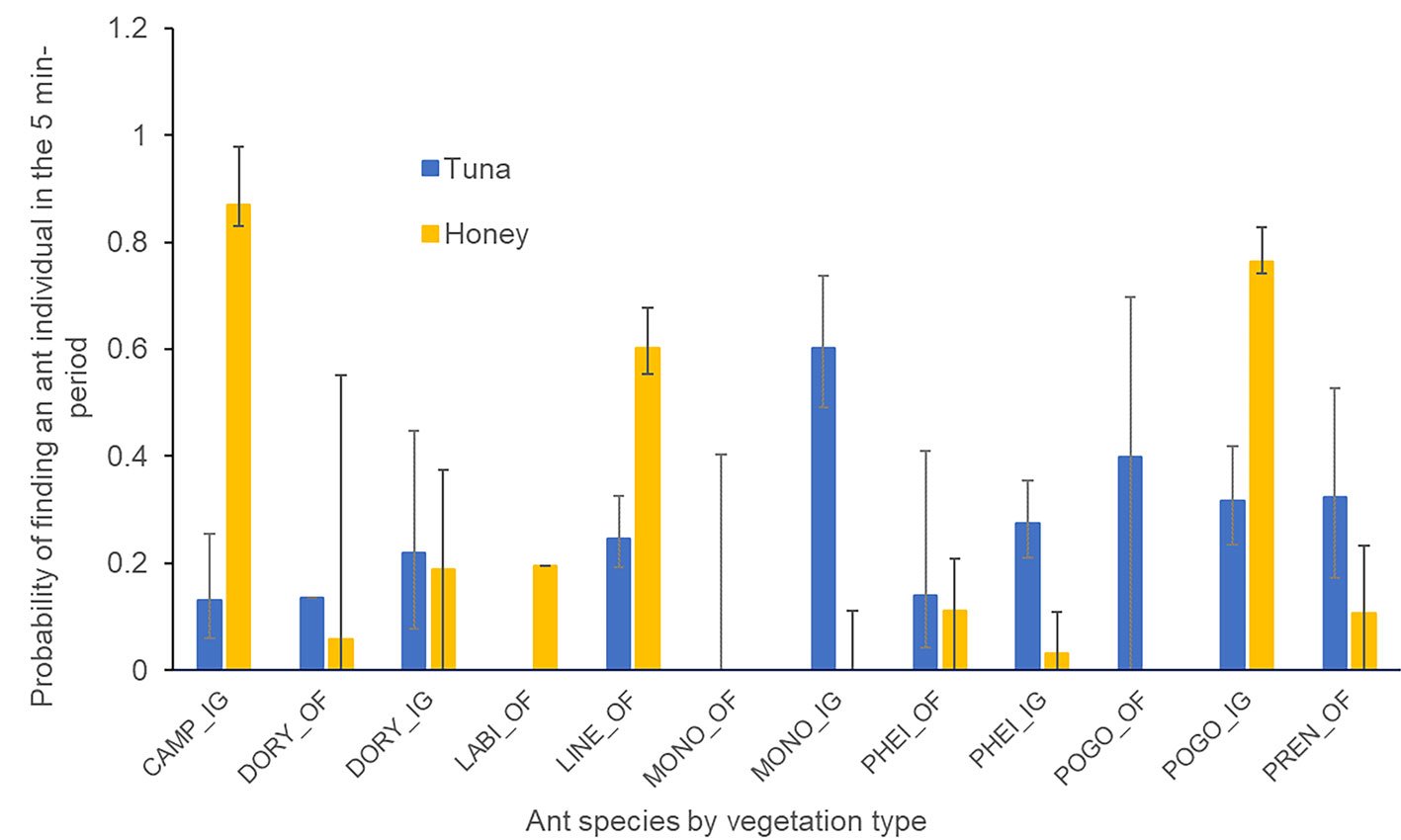
Figure 3. Probability of finding an ant forager on the honey or tuna baits at the nest of the different ant species registered in the Oak Forest (OF) and the Induced Grassland (IG) in the 5-minute period. CAMPO: Camponotus rubrithorax, DORY: Dorymyrmex insanus, LABI: Labidus coecus, LINE: Linepithema dispertitum, MONO: Monomorium ebenium, PHEI: Pheidole spp., POGO: Pogonomyrmex barbatus, PREN: Prenolepis imparis.

Figure 4. Survival curves depicting the arrival times of ant foragers on the baits (tuna or honey) during a one-hour observation.
No significant differences were found in the arrival times among ant species.
No significant differences were found in the arrival times between the vegetation types (x2 = 0.4, df = 1, p = 0.5). Moreover, no significant differences were found in the arrival times among the different ant species (x2 = 7.6, df = 7, p = 0.4) or the type of bait (x2 = 0.01, df = 1, p = 0.9; Fig. 4).
In the dominance index baits 12 ant morphospecies were recorded and different ant morphospecies were recorded in each of the vegetation types (Table 3). When comparing the average dominance index (DI) by vegetation type (mean ± SE, n; oak forest DI = 0.372 ± 0.071, 33; induced grassland DI = 0.251 ± 0.052, 44), was not statistically different (t= 1.091; df = 75; p = 0.2787), which would suggest a submissive behavior in both types of vegetation. Average dominance index by ant species indicates that M. ebenium, P. imparis and Pheidole sp. 3 behave as submissive in both vegetation types (t = 0.590, df = 20, p = 0.5617; t = -0.237, df = 10, p = 0.8171; t = -0.315, df = 11, p = 0.7590, respectively) (Table 4). It was not possible to compare the DI between vegetation types for Temnothorax sp., T. augusti, C. rubrithorax, N. austroccidua, L. dispertitum, D. insanus or P. pallidus, because they were only present in one of the vegetation types (Table 4).
The average dominance index for each ant species was low suggesting that all of them displayed submissive behaviors (F8,68 = 1.949, p = 0.06). Nylanderia austroccidua and L. dispertitum had the highest dominance indices, although it should be noted that N. austroccidua only had one record and L. dispertitum had 3 records. Additionally, Monomorium ebenium showed a tendency to behave as dominant (Table 4).
When comparing the mean dominance index by bait type, no significant differences were found (t = 1.023, df = 110, p = 0.3088; mean ± SE, n; tuna = 0.382 ± 0.060, 55; honey = 0.295 ± 0.053, 57). This indicates that ants exhibited submissive behavior in both types of bait.
According to the average dominance index per ant species in relation to the bait type, Pheidole sp. 3, P. imparis, M. ebeninum, C. rubrithorax, and D. insanus exhibited a submissive behavior in both types of baits (t = 0.888, df = 13, p = 0.3907; t= 0.988, df = 15, p = 0.3388; t = 0.189, df = 32, p = 0.8513; t = -0.918, df = 24, p = 0.3675, t = 2.390, df = 5, p = 0.0624, respectively) (Table 5) and L. dispertitum exhibited a dominant behavior in both types of baits (t = 0.421, df = 3, p = 0.7021).
Temnothorax sp. and P. pallidus were not compared statistically due to the low incidence registered; nonetheless, they presented a submissive behavior index in both types of bait. Neither T. augusti nor N. austroccidua were included in this analysis, as they were only present on the honey bait. In none of the species was there a difference in behavior between the baits.
Table 2
Number of nests found in the oak forest and the induced grassland.
| Species | Oak forest | Induced grassland |
| Camponotus rubrithorax | 0 | 3 |
| Dorymyrmex insanus | 4 | 6 |
| Labidus coecus | 1 | 0 |
| Linepithema dispertitum | 2 | 0 |
| Pheidole spp. | 7 | 6 |
| Pogonomyrmex barbatus | 1 | 2 |
| Prenolepis imparis | 3 | 0 |
| Monomorium ebenium | 1 | 1 |
Discussion
This study found that certain ant species (e.g., C. rubrithorax, L. dispertitum, P. barbatus) exhibited a preference for honey within specific vegetation types when compared to the rest of the ant community. The compensation hypothesis (Davidson, 2005; Kaspari & Yanoviak, 2001) predicts that the attractiveness of a nutrient to an organism is higher the more limiting it is. It is possible that this result is related to the fact that sugar is generally less available on the ground strata than protein (Kaspari & Yanoviak, 2001; Kaspari et al., 2012).
However, when considering the overall community level, no noticeable food preferences were found between the ant communities in the oak forest and the induced grassland vegetation. This lack of preference was evident both in the items carried to their nests and the resources provided on the baits. There were no significant differences in arrival times at the baits between vegetation types. This similarity can be attributed to ants experiencing soil-level heterogeneity similarly in both oak forests and induced grasslands (see below).
The ant communities in both habitats were composed of ant species displaying submissive behavior. This characteristic could be attributed to stress factors such as low temperatures in the oak forest and disturbances in the induced grassland, which potentially reduce ant competition. In the oak forest, low temperatures may favor the presence of cold climate specialists that can forage at low temperatures without the need to display a dominant behavior. In the induced grassland, disturbances may favor the presence of generalist species that take advantage of the absence of dominant species such as the dominant Dolichoderinae (see below). This study emphasizes the significance of ant species’ response to their environment and their adaptability in dealing with disturbances.
Our findings do not provide support for vegetation-scale disparities in food preferences, first and second hypotheses, which proposed greater differences in the food items being carried to the nest in the oak forest and reduced food preferences in the induced grassland. There were no differences between vegetation types in the number of seeds, plants, or arthropods taken by the ant foragers to their nests. Similarly, there was not a preference for a specific food bait (honey or tuna) between the oak forest and induced grassland ant communities. These findings are consistent with previous studies conducted by Radnan et al. (2018) and Castillo-Guevara et al. (2019), which did not identify differences in food preferences or foraging strategies between natural and disturbed vegetation at the community level. However, our observations did reveal that certain ant species exhibited preferences for specific types of food, within particular vegetation types, in accordance with the first hypothesis and second hypothesis but at the species level, which proposed an influence of ant species on food preferences. The specific preferences of these ant species are discussed in detail below.
Table 3
Visit frequency (i.e., number of foragers) per species in each vegetation type and functional groups they belong to (Andersen, 2000). GM = Generalized Myrmicinae, CCS = cold climate specialist, SC = subordinate Camponotini, TCS = tropical climate specialist, O = opportunist.
| Subfamily | Specie | Funtional group | Oak forest | Induced grassland |
| Myrmicinae | Monomorium ebenium | GM | 753 | 167 |
| Myrmicinae | Pheidole sp. 3 | GM | 14 | 236 |
| Myrmicinae | Temnothorax sp. | CCS | 5 | 0 |
| Myrmicinae | Temnothorax augusti | CCS | 0 | 1 |
| Formicinae | Prenolepis imparis | CCS | 289 | 11 |
| Formicinae | Camponotus rubrithorax | SC | 0 | 351 |
| Formicinae | Nylanderia austroccidua | TCS | 0 | 30 |
| Dolichoderinae | Linepithema dispertitum | CCS | 190 | 0 |
| Dolichoderinae | Dorymyrmex insanus | O | 0 | 26 |
| Pseudomyrmecinae | Pseudomyrmex pallidus | TCS | 0 | 10 |
| Total | 1,251 | 832 |
Table 4
Average numerical dominance index (DI) (mean ± SE, n) per ant morphospecies. (-) Unregistered species.
| Specie | Oak forest | Induced grassland | ID |
| Monomorium ebenium | 0.4 ± 0.1, 13 | 0.3 ± 0.1, 9 | 0.4 ± 0.0, 22 |
| Pheidole sp.3 | 0.2 ± 0.2, 4 | 0.2 ± 0.1, 9 | 0.2 ± 0.1, 13 |
| Temnothorax sp. | 0 ± 0, 3 | – | 0 ± 0, 3 |
| Temnothorax augusti | – | 0, 1 | 0 ± 0, 1 |
| Prenolepis imparis | 0.3 ± 0.1, 10 | 0.5 ± 0.5, 2 | 0.3 ± 0.1, 12 |
| Camponotus rubrithorax | – | 0.1 ± 0.0, 15 | 0.1 ± 0.0, 15 |
| Nylanderia austroccidua | – | 1, 1 | 1, 1 |
| Linepithema dispertitum | 0.7 ± 0.1, 3 | – | 0.7 ± 0.1, 3 |
| Dorymyrmex insanus | – | 0.2 ± 0.1, 4 | 0.3 ± 0.1, 4 |
| Pseudomyrmex pallidus | – | 0 ± 0, 3 | 0 ± 0, 3 |
Pheidole spp., in the induced grassland, were observed carrying a greater quantity of plant elements to their nests in both vegetation types. However, it exhibited a preference for the tuna bait in induced grassland, possibly indicating a supplementary dietary preference. Given the extensive diversity within the Pheidole genus, which encompasses 900 species described worldwide (Wilson, 2003), it is not feasible to categorize them based on a specific food habit and our results suggest that it is omnivorous (Table 6). Nevertheless, these results should be interpreted with caution due to the grouping of species.
Camponotus rubrithorax and P. barbatus, in the induced grassland, as well as L. dispertitum, in the oak forest, were more frequently observed foraging the honey bait compared to other ant species. Camponotus (Mayr) is a genus known for its nectarivorous habits and consumption of other sweet secretions, such as honeydew which coincides with its preference for honey found in the present study (Nettimi & Iyer, 2015). In this study, L. dispertitum predominantly consumed honey, although it is a generalist forager species capable of consuming other types of food as well (Table 5), in the study site it is found exclusively in the oak forest (Cuautle et al., 2016).
Despite Pogonomyrmex (Mayr) has been recognized as a granivorous genus (Pirk & López-de Casenave, 2014), this study provided new insights into the foraging preferences of P. barbatus, revealing a notable inclination towards carbohydrates and plant elements within the induced grassland. Moreover, we even registered individuals transporting arthropods to their nests. These findings (Table 5) strongly indicate that certain species within the Pogonomyrmex genus exhibit a generalist foraging behavior. Other species such as D. insanus, which used resources more intensively in the induced grassland, showed no preference for any of the baits or items taken to the nest, which coincides with the generalist forager behavior, observed in open and disturbed habitats by Cuezzo and Guerrero (2012).
Table 5
Average numerical dominance index (DI) (mean ± SE, n) per ant species in both bait types (tuna, honey). (-) Unregistered species.
| Species | Tuna | Honey |
| Monomorium ebenium | 0.4 ± 0.1, 18 | 0.4 ± 0.1, 16 |
| Pheidole sp.3 | 0.4 ± 0.2, 7 | 0.1 ± 0.1, 8 |
| Temnothorax sp. | 0, 1 | 0 ± 0, 2 |
| Temnothorax augusti | – | 0, 1 |
| Prenolepis imparis | 0.5 ± 0.1, 7 | 0.3 ± 0.1, 10 |
| Camponotus rubrithorax | 0.1 ± 0.0, 14 | 0.2 ± 0.0, 12 |
| Nylanderia austroccidua | – | 1, 1 |
| Linepithema dispertitum | 0.7 ± 0.2, 2 | 0.6 ± 0.3, 3 |
| Dorymirmex insanus | 0.6 ± 0.3, 3 | 0 ± 0, 4 |
| Pseudomyrmex pallidus | 0 ± 0, 3 | 0, 1 |
Table 6
The biology and ecology of the ant genera found in this study, in the Flor del Bosque State Park (Agosti et al., 2000; AntWiki, n.d.).
| Genera | Microhabitat | Food habits |
| Camponotus | Ground nesting, decaying wood and in trees | Generalist foragers |
| Dorymyrmex | ————– | Generalist foragers |
| Linepithema | ————– | Generalist foragers |
| Labidus | Epigeous,bivouacs | Predators (Army ants) |
| Monomorium | ————– | Generalized foragers, harvesters |
| Nylanderia | Nest in leaf litter, soil, or in rotten wood | Generalist foragers |
| Pheidole | Soil or decaying wood | Granivores or omnivores |
| Pogonomyrmex | Ground nesting | Generalist foragers and granivores |
| Prenolepis | ————– | Generalist predators |
| Pseudomyrmex | Mostly arboreal (nesters and foragers), few epigaeic | Generalized predators, visit extrafloral nectaries |
| Temnothorax | Nesting in ground, and under stones, in wood, and in trees | Generalized foragers and parasites |
The previous results (e.g., C. rubrithorax, Pheidole spp., D. insanus) support the reported food habits of specific ant genera. Nonetheless, it is also possible to interpret these results as ants taking nutrients from the baits that are not currently available or that are limited within their community to supplement their diet (Compensation hypothesis) (Davidson, 2005; Kaspari & Yanoviak, 2001). In this study, significant differences in ant species presence on baits were primarily associated with the presence of ant species on honey baits. This finding aligns with the compensation hypothesis (Davidson, 2005; Kaspari & Yanoviak, 2001), which posits that the utility of a resource remains constant across species and varies solely with availability. The hypothesis predicts a singular limiting resource that is locally in shortest supply. Consequently, habitats with relatively high protein availability should attract ants more inclined towards carbohydrates, and vice versa. Previous research has demonstrated that litter ant communities are limited by carbohydrates, whereas ant arboreal communities face protein limitations in tropical regions (Kaspari & Yanoviak, 2001; Kaspari et al., 2012). Although this study was conducted in a temperate environment, the results might be related to the usual scarcity of sugar in the ground strata compared to protein.
Our results do not align with the second hypothesis, which speculated faster arrival times in the induced grassland. We did not find significant differences in arrival times among vegetation types, ant species, or bait types. Ants could be experiencing similar heterogeneities at the soil level between the oak forest and induced grassland. While it is expected that the presence of more litter in the oak forest could hinder ant movement, within the induced grassland, the vegetation morphology itself (long grass species) could be interfering with ant movement. For instance, Hernández-Flores et al. (2016) observed that the foraging performance of P. barbatus was reduced due to the presence of herbaceous vegetation in plots where regeneration after grazing was permitted.
Dominance hierarchy. Disturbance typically favors the presence of generalist and opportunistic species, hence, we expected to find a lower dominance index within the induced grassland (third hypothesis). Nonetheless, we did not find enough evidence to support this hypothesis as we registered ant communities consisted of submissive species in both habitats. Additionally, the ants did not show a tendency to dominate a specific resource, neither at the bait level nor at the species level, suggesting a lack of food preferences. These results are consistent with the findings of Castillo-Guevara et al. (2019), who registered no significant differences in dominance indices between a native oak forest and an altered agricultural land. Moreover, the authors reported intermediate to low values of dominance within the ant communities of each vegetation type. Our findings could be attributed to the presence of other factors that could have overshadowed the role of competition in shaping the organization of ant communities. For example, a review by Parr and Gibb (2012), which encompassed data from 3 continents, indicated that the trade-off between discovery and dominance occurs primarily when parasitoids are present. In environments without parasitoids, species with high discovery abilities tend to also be dominant (Parr & Gibb, 2012). While our study did not specifically assess the discovery-dominance trade-off, the observed lack of differences in arrival times and similar dominance values among the ants suggest that dominance was not a prominent factor in our study sites. It is possible that factors such as low temperatures in the oak forest, or disturbance in the induced grassland, may have played a role in relaxing dominance. According to Andersen (2000), in disturbed vegetation like the induced grassland, it is expected to observe the presence of subdominant ant species that exploit the absence of dominant species from the native vegetation, such as dominant Dolichoderinae. The findings obtained during this study align with this prediction and provide support for it. Notwithstanding, the absence of ants with high dominance indices in the studied communities does not necessarily indicate a complete lack of dominance hierarchy. In each community, the ants can still be ordered based on their DI. For example, in the oak forest, L. dispertitum had the highest DI value (0.7 DI), M. ebenium had an intermediate value (0.4 DI) and Temnothorax spp. had the lowest value (0.0 DI).
Land use change did not seem to influence food preferences or foraging strategies at the community level. However, we observed an effect at species level, indicating that individual ant species exhibited specific food preferences. Carbohydrates could be the limiting resource in the oak forest and the induced grassland litter ant communities, as some ant species showed preference for honey baits. Although competition is typically considered a key factor in understanding food preferences among ants, it is noteworthy that both, the natural oak forest and induced grassland, were predominantly populated by submissive ant species. Therefore, it appears that other factors instead of competition may be playing a role in shaping food preferences within these communities. In conclusion, our study reveals that ant species may exhibit preferences for specific foods, which could be limited in their environment. The ability of ants to respond to available resources enables them to optimize their nutrient intake, as well as adapt and persist under variable conditions, including disturbances. Understanding the distinct dietary preferences and foraging strategies of ant species within functional groups will provide valuable insights into their ecological roles and potential impacts on ecosystem dynamics. Such investigations would enhance our ability to predict the responses of ants to diverse forms of disturbances in an anthropized world.
Acknowledgements
We appreciate the assistance provided by the authorities of “Flor del Bosque” State Park, coordinator Enrique Martínez Romero (M.S.) and director Mario Alberto Romero Guzmán (MVZ). We would also like to thank Florencio Luna Castellanos for his support with the fieldwork. This study was financed by Consejo Nacional de Humanidades Ciencias y Tecnologías (Conahcyt) as part of a grant awarded to Mariana Cuautle (223033).
References
Abacus Concepts Inc. (1996). Abacus Concepts, Stat View Reference. Berkeley, California.
Agosti, D., Majer, J. D., Alonso, L. E., & Schultz, T. R. (2000). Ants: standard methods for measuring and monitoring bio-
diversity. Washington D.C.: Smithsonian Institution Press.
Andersen, A. (2000). A global ecology of rainforest ants: functional groups in relation to environmental stress and disturbance. In D. Agosti, J. D. Majer, L. E. Alonso, & T. R. Schultz (Eds.), Ants: standard methods for measuring and monitoring biodiversity (pp. 25–34). Washington D.C.: Smithsonian Institution Press.
Andersen, A.N. (1992). Regulation of “momentary” diversity by dominant species in exceptionally rich ant communities of the Australian seasonal tropics. The American Naturalist, 40, 401–420. https://www.journals.uchicago.edu/doi/abs/10.
1086/285419
AntWiki (n.d.). Nylanderia. AntWiki. Consulted 8/20/2024
Arnan, X., Cerdá, X., & Retana, J. (2012). Distinctive life traits and distribution along environmental gradients of dominant and subordinate Mediterranean ant species. Oecologia, 170, 489–500. https://doi.org/10.1007/s00442-012-2315-y
Castillo-Guevara, C., Cuautle, M., Lara, C., & Juárez-Juárez, B. (2019). Effect of agricultural land-use change on ant dominance hierarchy and food preferences in a temperate oak forest. PeerJ, 7, e6255. https://peerj.com/articles/6255/
Cerdá, X., Arnan, X., & Retana, J. (2013). Is competition a significant hallmark of ant (Hymenoptera: Formicidae) ecology? Myrmecological News, 18, 131–147. https://doi.org/10.25849/myrmecol.news_018:131
Cerdá, X., Retana, J., & Cros S. (1997). Thermal disruption of transitive hierarchies in Mediterranean ant communities. Journal of Animal Ecology, 66, 363–374.
Costes-Quijano, R., Meza, A. R., Macías-Juárez, A., Berriel-Mastreta, C. A., Cortés-Atilano, B., Martínez-Romero, L. E. et al. (2006). Plan de manejo Parque Ecológico Recreativo General Lázaro Cárdenas “Flor del Bosque”. [Management Plan of the recreative ecological Park “General Lázaro Cárdenas “Flor del Bosque”]. Ciudad de México: Gobierno del Estado de Puebla/ Secretaría de Medio Ambiente y Recursos Naturales.
Cuautle, M., Vergara, C., & Badano, E. (2016). Comparison of ant community diversity and functional group composition associated to land use change in a seasonally dry oak forest. Neotropical Entomology, 45, 170–9. https://doi.org/
10.1155/2012/516058
Cuezzo, F., & Guerrero, R. J. (2012). The Ant Genus Dorymyrmex Mayr (Hymenoptera: Formicidae: Dolicho-
derinae) in Colombia. Psyche, 51605, 1–24. https://doi.org/
10.1155/2012/516058
Dáttilo, W., Díaz-Castelazo, C., & Rico-Gray, V. (2014). Ant dominance hierarchy determines the nested pattern in ant-plant networks. Biological Journal of the Linnean Society, 113, 405–414. https://doi.org/10.1111/bij.12350.
Davidson, D. W. (2005). Ecological stoichiometry of ants in a New World rain forest. Oecologia, 142, 221–231. https://doi.org/10.1007/s00442-004-1722-0
Dejean, A., & Corbara, B. (2003). A review of mosaics of dominant ants in rainforests and plantations. In Y. Basset, V. Novotny, S. E. Miller, & R. L. Kitching (Eds.), Arthropods of tropical forests: spatio-temporal dynamics and resource use in the canopy (pp 341–347). Cambridge: Cambridge University Press.
Ellis, E. C., Goldewijk, K. K., Siebert S., Lightman, D., & Ramankutty, N. (2010). Anthropogenic transformation of
the biomes, 1700 to 2000. Global Ecology and Biogeo-
graphy, 19, 589–606. https://doi.org/10.1111/j.1466-8238.20
10.00540.x
Fellers, J. H. (1987). Interference and exploitation in a guild of Woodland ants. Ecology, 68, 1466–1478. https://doi.org/
10.2307/1939230
Fellers, J. H. (1989). Daily and seasonal activity in woodland
ants. Oecologia, 78, 69–76. https://doi.org/10.1007/BF0037
7199
Foley, J. A., DeFries, R., Asner, G. P., Barford C., Bonan, G., Carpenter, S. R. et al. (2005). Global consequences of land use. Science, 309, 570–574. https://doi/10.1126/science.1111772
Hoffmann, B. D., & Andersen, A. N. (2003). Responses of ants to disturbance in Australia, with particular reference to functional groups. Austral Ecologyl, 28, 444–464. –https://doi.org/10.1046/j.1442-9993.2003.01301.x
Houdria, M., Salas-López, A., Orivel. J., Bluthgen, N., & Menzel, F. (2015). Dietary and temporal niche differentiation in tropical ants – can they explain local ant coexistence? Biotropica, 47,208–217. https://doi.org/10.1111/btp.12184
Hernández-Flores, J., Osorio-Beristain. M., & Martínez-Garza. C. (2016). Ant foraging as an indicator of tropical dry forest restoration. Environmental Entomology, 45, 991–994. https://doi.org/10.1093/ee/nvw054
Kaspari, M., Donoso, D., Lucas, J. A., Zumbusch, T., & Kay, A. D. (2012). Using nutritional ecology to predict community structure: a field test in Neotropical ants. Ecosphere, 3,93. https://doi.org/10.1890/ES12-00136.1
Kaspari, M., & Yanoviak, S. P. (2001). Bait use in tropical litter and canopy ants-evidence of differences in nutrient limitation. Biotropica, 33,207–211. https://doi.org/10.1646/
0006-3606(2001)033[0207:BUITLA]2.0.CO;2
Łaska, G. (2001). The disturbance and vegetation dynamics: a review and an alternative framework. Plant Ecology, 157, 77–99. https://doi.org/10.1023/A:1013760320805
Lynch, J. F., Balinsky, E. C., & Vail, S. G. (1980). Foraging patterns in three sympatric forest ant species, Prenolepis imparis, Paratrechina melanderi and Aphaenogaster rudis (Hymenoptera: Formicidae). Ecological Entomology, 5,353–371. https://doi.org/10.1111/j.1365-2311.1980.tb01160.x
Mackay, W., & Mackay, E. (1989). Clave de los géneros de hormigas en México (Hymenoptera: Formicidae). El Paso, Texas: The University of Texas.
Nettimi, R. P., & Iyer, P. (2015). Patch fidelity in Camponotus compressus ants foraging on honeydew secreted by treehoppers. Current Science, 109, 362–366.
Parr, C. L. (2008). Dominant ants can control assemblage species richness in a South Africa savanna. Journal of Animal Ecology, 77, 1191–1198. https://doi.org/10.1111/j.13
65-2656.2008.01450.x
Parr, L., & Gibb, H. (2012). The discovery-dominance trade-off
is the exception, rather than the rule Journal of Animal
Ecology, 81, 233–241. https://doi.org/10.1111/j.1365-2656.
2011.01899.x
Pirk, G. I., & López-de Casenave, J. (2014). Effect of harvester ants of the genus Pogonomyrmex on the soil seed bank around their nests in the central Monte desert, Argentina. Ecological Entomology, 39, 610–619. https://doi.org/10.1111/een.12140
R Core Team (2022). R: a language and environment for statistical computing. Vienna, Austria: R Foundation
for Statistical Computing. https://www.R-project.org/
Radnan, G. N., Gibb, H., & Eldridge, D. J. (2018). Soil surface complexity has a larger effect on food exploitation by ants than a change from grassland to shrubland. Ecological Entomology, 43, 379–388. https://doi.org/10.1111/een.12510
Rico-Gray, V., & Oliveira, P. S. (2007). The ecology and evolution of ant-plant interactions. Chicago: University of Chicago Press.
Sala, O. E., Chapin, F. S., Armesto, J. J., Berlow, E., Bloomfield, J., Dirzo. R. et al. (2000). Global biodiversity scenarios for the year 2100. Science, 287,1770–1774. https://doi.org/10.1126/science.287.5459.17
Santini, G., Tucci, L., Ottonetti, L., & Frizzi, L. (2007). Competition trade-offs in the organisation of a Medite-
rranean ant assemblage. Ecological Entomology, 32,
319–326. https://doi.org/10.1111/j.1365-2311.2007.00882.x
Savolainen, R., Vepsäläinen, K., & Wuorenrinne, H. (1989). Ant assemblages in the taiga biome: testing the role of territorial wood ants. Oecologia, 81, 481–486. https://doi.org/10.1007/BF00378955

The sounds of love: acoustic repertoire of Andean bear, Tremarctos ornatus (Carnivora: Ursidae), mating in the wild
Adriana Reyes a, b, Nicolás Reyes-Amaya a, b, Ramiro Velazco c, Manuel Meneses c, Andrés Cortés e, Katherine Arenas-Rodríguez d, Edward Rojas e, Ximena Velez-Liendo f, Angela M. Mendoza-Henao a, *
a Instituto de Investigación de Recursos Biológicos Alexander von Humboldt, Centro de Colecciones y Gestión de Especies, Colecciones Biológicas, Carrera 8 No. 15 – 08, 154001 Villa de Leyva, Colombia
b Fundación para la Investigación, Conservación y Protección del Oso Andino (Fundación Wii), Calle 161, 12C-30, 110131 Bogotá, Colombia
c Grupo de monitoreo comunitario Serankwa, Vereda Candela, San Agustín, Huila, Colombia
d Corporación Autónoma Regional del Alto Magdalena, Carrera 1 No. 60-70, Neiva, 41797 Huila, Colombia
e Corporación Autónoma Regional de Cundinamarca, Dirección Recursos Naturales, Calle 24 No. 60-50, Bogotá, Colombia
f University of Oxford, Department of Biology, Wildlife Conservation Research Unit, Recanati-Kaplan Centre, Tubney House Abingdon Road, Tubney, Oxfordshire, OX13 5QL United Kingdom
*Corresponding author: am.mendozah@gmail.com (A.M. Mendoza-Henao)
Received: 14 March 2024; accepted: 11 October 2024
Abstract
Understanding animal behavior is crucial for effective mammal conservation efforts; however, limited knowledge exists regarding the behavioral patterns of many species, particularly in wild conditions. The Andean bear (Tremarctos ornatus) is the only ursid distributed in South America and is categorized as vulnerable to extinction by the IUCN. The information on various aspects of its natural history in wildlife conditions are scarce, including the ethology of its reproduction. In this study, we describe the sound repertoire emitted by T. ornatus during copulation and mating events in their natural habitat. Video recordings obtained from camera traps in Colombia and Bolivia were analyzed to identify and categorize vocalizations. The results revealed 5 distinct types of sounds emitted during copulation events: humm, grunt, whine, and snoar signals. Differences in vocalization patterns were observed between the male and female bears. Comparisons with existing literature suggest similarities with the vocalizations observed for other species. This study contributes valuable information to the understanding of Andean bear behavior and underscores the importance of acoustic communication in conservation efforts for cryptic species.
Keywords: Camera trapping; Colombia; Bolivia; Bioacoustics; Reproductive behaviour
© 2025 Universidad Nacional Autónoma de México, Instituto de Biología. Este es un artículo Open Access bajo la licencia CC BY-NC-ND
(http://creativecommons.org/licenses/by-nc-nd/4.0/).
Sonidos amor-osos: repertorio acústico del oso andino Tremarctos ornatus (Carnivora: Ursidae) durante el apareamiento en vida silvestre
Resumen
Comprender el comportamiento de los animales es crucial para que los esfuerzos de conservación de los mamíferos sean eficaces, pero los conocimientos sobre los patrones de comportamiento de muchas especies, sobre todo en condiciones salvajes, son limitados. El oso andino (Tremarctos ornatus) es el único úrsido distribuido en Sudamérica, categorizado como vulnerable a la extinción por la UICN. La información sobre diversos aspectos de su historia natural en vida silvestre es escasa, incluyendo la etología de su reproducción. En este estudio describimos el repertorio sonoro emitido durante los eventos de cópula y apareamiento por T. ornatus en su hábitat natural. Se analizaron grabaciones de vídeo obtenidas con cámaras trampa en Colombia y Bolivia para identificar y categorizar las vocalizaciones. Los resultados revelan 5 tipos distintos de sonidos emitidos durante los eventos de cópula, incluyendo señales de “humm”, “grunt”, “whine” y “snoar”. Se observaron diferencias en los patrones de vocalización entre machos y hembras. Las comparaciones con la literatura existente sugieren similitudes con las vocalizaciones observadas en otras especies. Este estudio contribuye con información valiosa a la comprensión del comportamiento del oso andino y subraya la importancia de la comunicación acústica en los esfuerzos de conservación de especies crípticas.
Palabras clave: Fototrampeo; Colombia; Bolivia; Bioacústica; Comportamiento reproductivo
Introduction
The study of animal behavior plays a fundamental role in mammalian conservation, as it provides valuable information on the relationships between species and their environment (Berger-Tal et al., 2016). Understanding species behavioral patterns is crucial for designing effective conservation strategies, as it allows scientists to identify and address key factors influencing population dynamics, habitat utilization, and overall ecological balance. A thorough understanding of animal behavior is essential for developing informed and adaptive conservation practices that safeguard species diversity. In many cases, knowledge of the behavior of wild species of large mammals comes from captive conditions (Jayne & See, 2019). Although captivity provides a controlled environment for observation, it can inadvertently influence animal behavior. Captive individuals exhibit altered behaviors as they are subjected to artificial conditions, restricted spaces, and stimuli provided by humans. This can lead to biased results that do not accurately reflect the natural behavior of their wild counterparts. Even so, information on wild conditions is scarce for many species, considering the difficulties in directing encounters without altering individual behavior.
Few studies have focused on the social behavior and vocalizations of ursids (Wemmer et al., 1976). The first studies on this subject were done by Meyer-Holzapfel (1957), who mentioned several calls of different species; Krott and Krott (1962) described the vocalizations of the European brown bear (Ursus arctos, Carnivora: Ursidae), and Jonkel (1970), Jonkel and Cowan (1971) described calls used in agonistic contexts by North American bears, while Negus (1949) in his study of the vertebrate larynx reported that bears are generally silent.
Fortunately, advances in remote sensing technologies have provided us with opportunities to explore animal behavior. The scarcity of information on the ecology of the Andean bear has been changing in recent years owing to the use of tools such as camera traps, which have allowed us to obtain more information about the species, and the recording of various behaviors such as courtship, maternal care, and copulation events has been achieved (Appleton et al., 2018; Castellanos, 2015; Reyes et al., 2018, 2024). The objective of this study was to describe the vocalizations emitted by Andean bears during copulation events in the wild.
Materials and methods
Video records were obtained using camera traps during the copulation of wild bears in 3 locations: 2 in Colombia and 1 in Bolivia (Fig. 1). The first was in the Department of Huila (Colombia): the mating event was recorded by the SERANKWA monitoring group in a Cuddeback camera trap located in the site called “El Rascadero” (1°49’35.06” N, 76°23’35.41” W, WGS84), in the Natural Reserve of the Civil Society La Loma del Toro Pao in the Municipality of San Agustín at 2,410 m asl, the reserve has areas of forest cover in good condition (Parques Nacionales Naturales de Colombia, 2017). The second locality was in the department of Cundinamarca (Colombia): this mating event was recorded by the Corporación Autónoma Regional de Cundinamarca- CAR, Dirección de Recursos Naturales, Grupo de Biodiversidad in 2 camera traps (Bushnell Trophy Cam HD) in the municipality of Guatavita (4°54’0.06” N; 73°44’21.56” W and 4°53’58.65” N, 73°43’40,47” W, WGS84), in the Eastern Cordillera (Anillo Oriental) of the Colombian Andes in the buffer zone of Chingaza Natural Park, which includes Andean and high Andean forests between 2,500 and 3,000 m asl. The third locality is in Tarija department (Bolivia): mating event was recorded in 2 camera traps (Bushnell Trophy Cam HD Aggressor) 15.8 km from Hoyadas Cercado, Cercado Province (21°7’29.10” S, 64°25’16.90” W and 21°14’39.00” S, 64°20’12.90” W, WGS84), between 930 and 3,400 m asl.

Figure 1. Location of study sites. A) El Rascadero, Huila, Colombia; B) Chingaza, Cundinamarca, Colombia; C) Cercado, Tarija, Bolivia. Map by Angela M. Mendoza-Henao.
The videos were manually examined to identify those with vocalizations and, to the extent possible, to assign the signal to the male or female. WAV files were generated from the selected videos. Information on the times of vocal activity was obtained from camera trap metadata. Acoustic parameters were obtained using Raven 1.6.2 (K. Lisa Yang Center for Conservation Bioacoustics): call duration, minimum and maximum frequency were obtained using 5% and 95% values with a window size of 1,024 and a Hann algorithm. The final recordings were deposited in the Colección de Sonidos Ambientales “Mauricio Álvarez-Rebolledo” of the Instituto de Investigación de Recursos Biológicos Alexander von Humboldt of Colombia (IAvH-CSA-37506 to IAvH-CSA-37510). The vocalization parameters were summarized and described for each event.
Results
Vocalizations or sounds were obtained from the 6 copulation events analyzed (3 from Colombia and 3 from Bolivia), with some differences in audio quality due to the camera trap brands and models, and the distance of the individuals from the equipment. During the analysis, we were able to classify 5 different types of sounds according to the shape of the spectrogram (Table 1), following the terminology of vocalization descriptions of other ursids (Peters et al., 2007; Pokrovskaya, 2013).
Regarding the Cundinamarca events in Colombia, mating occurred on September 14, 2021, between 11:36 and 12:33 hrs. (camera 4), and between 14:24 and 15:51 hrs. (camera 5). Acoustic signals were detected in 55 videos from both sites (Fig. 2). All the sounds recorded were presented when the male is on the female, in the videos it is observed how both the male and the female emit different sounds in the process of copulation. In general, all the recorded sounds are of the copulation process. A total of 33 sounds between vocalizations and snorts were emitted by females and 48 by males. For the remaining vocalizations, individual correspondence could not be verified. The bears mostly emitted humm-type vocalizations, which in some cases were preceded or followed by other types of vocalizations. During the time of copulation, both videos and sounds show some moments of aggressiveness of the male towards the female, this is evident in an event where the male bites the neck of the female and she emits a very high-pitched sound (bite-type vocalization, Fig. 2). Table 2 summarizes the main quantified parameters of the signals.
For events in Bolivia, 2 videos from station PI072 included sound information (Fig. 3a). The recorded vocalizations included humm, grunt and whine signals emitted simultaneously by males and females. Snort-type vocalizations were dominant in both the recordings. These recordings provided information on frequencies below 5 kHz, and harmonics up to 10.16 kHz in frequency were detected. Four of the videos from station PI012 included sounds from a single individual in sight (Fig. 3b), recorded at 6:42 am and between 10:37 am and 10:41 am. All signals were humm with 9 – 22 pulses with a dominant frequency at 344.53 ± 54.47 Hz and a second harmonic frequency with the highest energy at 6,488.67 ± 611.07 Hz with frequencies covering a bandwidth of 8,641.99 ± 886.23 Hz. The mean signal duration was 1.035 ± 0.33 s. Finally, a single video from station PI071 from 2022-10-29 includes a series of sounds made by a single individual (sex unknown, Fig. 3c) including humm (dominant frequency of 301.46 Hz and duration of 0.96 s), whine (dominant frequency of 172.2, duration of 3.52 s) and snoar (dominant frequency at 3,200 Hz for 2 signals and 872.1 for the remaining 4, total duration of 0.255 s) type signals.

Figure 2. Spectrograms of the 6 types of Tremarctos ornatus signals emitted during the mating event in Cundinamarca, Colombia.
The mating event in Huila (Colombia) occurred on February 9, 2020, between 08:14 and 13:03 hrs. The second copulation event was recorded at the same site on February 13, 2020, between 14:05 and 17:17 hrs. (56 videos and 49 photographs). The camera had a sound filter above 5 kHz, which limited the availability of data beyond this frequency. Acoustic signals were detected in only 28 of 122 videos. Five videos in the interval between the 2 mating events also had acoustic signals. Owing to the sound quality of the camera and the distance of the pair, the signal was sufficient in only 1 video to extract some spectral parameters (Fig. 4). In this case, the call was probably a 2.196 second humm-type vocalization, with frequencies between 1,125.0 and 1,843.75 Hz (dominant frequency 1,625.00 Hz).
Table 1
Description of the type of acoustic signals of Tremarctos ornatus during courtship and copulation events and spectrogram example of each one (1 second section).

Table 2
Summary of the main signal parameters for mating in Cundinamarca (Colombia). Spectral values are given in Hz and signal duration in seconds. Values for more than 3 signals mean ± standard deviation.
| Type | Sex | N | Dom freq | Min freq | Max freq | Freq bandwidth | Signal duration |
| Bite | F | 2 | 1,679.55 ± 1,888.05 | 301.45 ± 121.83 | 2,045.65 ± 1,979.40 | 1,744.20 ± 1,857.57 | 0.550 ± 0.495 |
| NA | 2 | 344.50 ± 0.00 | 193.80 ± 30.41 | 925.95 ± 700.39 | 732.15 ± 730.79 | 1.650 ± 0.071 | |
| Grunt | M | 8 | 220.70 ± 101.49 | 134.58 ± 104.09 | 613.70 ± 713.54 | 479.13 ± 610.10 | 0.213 ± 0.164 |
| NA | 14 | 196.88 ± 62.55 | 153.81 ± 43.78 | 310.69 ± 117.26 | 156.88 ± 90.36 | 0.407 ± 0.327 | |
| Whine | F | 5 | 516.78 ± 337.73 | 353.14 ± 47.19 | 1,326.44 ± 315.59 | 973.30 ± 309.94 | 0.420 ± 0.409 |
| NA | 41 | 259.45 ± 101.22 | 199.58 ± 73.82 | 638.65 ± 627.49 | 439.06 ± 589.26 | 0.478 ± 0.442 | |
| Humm | F | 25 | 821.70 ± 1,090.34 | 246.35 ± 82.02 | 2,322.15 ± 1,024.95 | 2,075.80 ± 1,002.38 | 2.112 ± 1.568 |
| M | 24 | 434.25 ± 545.76 | 254.81 ± 175.48 | 1,492.98 ± 1,132.87 | 1,238.17 ± 1,059.89 | 1.071 ± 0.765 | |
| NA | 310 | 329.52 ± 224.89 | 229.37 ± 59.32 | 1,149.46 ± 853.06 | 920.10 ± 847.90 | 1.331 ± 0.791 | |
| Snoar | F | 1 | 344.50 | 301.5 | 1,507.30 | 1,205.8 | 1.2 |
| M | 16 | 788.64 ± 1,100.30 | 183.03 ± 172.63 | 1,924.53 ± 1,430.22 | 1,741.50 ± 1,346.52 | 0.275 ± 0.284 | |
| NA | 5 | 1,834.60 ± 1,522.19 | 611.54 ± 532.20 | 3,307.48 ± 1,172.88 | 2,695.94 ± 1,110.42 | 0.240 ± 0.114 |

Figure 3. Mating events and spectrograms of Tremarctos ornatus signals emitted during the mating event in Tarija, Bolivia. a) Camera PI072, b) camera PI012 y c) camera PI071.

Figure 4. Mating events and spectrogram of Tremarctos ornatus signals emitted during the mating event in Huila, Colombia.
Discussion
This study provides the first description of the acoustic mating repertoire of T. ornatus based on quantitative measurements of in-situ vocalizations. In general, for ursids, some descriptions of vocalizations correspond to verbal or onomatopoeia-based descriptions (Pokrovskaya, 2013), which makes it difficult to make rigorous quantitative comparisons between species or between different social contexts of communication. For example, Castellanos et al. (2005) differentiated 6 sound types for 2 T. ornatus individuals in the process of reintroduction. Following Pokrovskaya’s (2013) synonyms of signal types, the sounds named by Castellanos et al. (2005) as guttural (kurrrrr or tuutuctttt) would be analogous to humm-like signals but could also correspond to a signal type called “chuffing” described for other ursids, with differences in structure in comparison to humm signals. Scream-like sounds could be analogous to bite but could also be referring to grunt type signals; short puffs would be analogous to snorts, and whines (eggmmmmmmmm) may be like whine. Given the limited nature of this differentiation and the lack of available recordings, it is impossible to make an assignment or rigorous comparison.
Knowledge of the vocalizations of this species has been restricted to captive conditions, especially from interactions between females and their cubs (Elowson, 1988; Peters et al., 2007). When comparing the available quantitative information, we found similarities in the frequencies of our humm-type signals (821.70 ± 1,090.34 Hz in females, 434.25 ± 545.76 Hz in males and 329.52 ± 224.89 Hz in undetermined cases) with the mother and pup signals termed trill (418 ± 39 Hz for mothers and 375 ± 104 Hz for pups). Grunt-type signals had slightly higher frequencies in our records (220.70 ± 101.49 Hz in females and 196.88 ± 62.55 Hz in indeterminate cases vs. 175 ± 35 Hz for mothers). Whimper-type sounds of cubs (347 ± 181 Hz) were within the frequency range of our records for whine-type signals (516.78 ± 337.73 Hz for females and 259.45 ± 101.22 Hz for indeterminate cases). It should be noted that it would be ideal to make spectrogram comparisons directly for a more detailed comparison, as the dominant frequency alone may not be sufficient for describing and comparing these signals.
In recent information on T. ornatus, Vela-Vargas et al. (2021) mentioned that vocalizations are composed of tonal and atonal elements with ranges from 0.01 to 7 kHz; however, they did not report the source of this statement. Based on the information obtained in the Bolivian camera traps in our study, we can identify harmonics at high frequencies, even up to 12 kHz, and the highest energy of the signals includes a frequency band of 8,641.99 ± 886.23 Hz. In this sense, our work reports a wider use of frequencies by T. ornatus than reported to date. This was made possible by the quality of sound recordings from the camera traps used at these sites, demonstrating that advances in the quality of audio recordings from the equipment can provide useful information on multiple aspects of the biology of these species.
The degree of vocalization of bears varies by species. Herrero (1978) suggested that black bears are more vocal than brown bears, because they inhabit denser vegetation and have restricted visibility. Historically, closed area ursids, such as Andean bears (Tremarctos ornatus), sloth bears (Melursus ursinus), and sun bears (Helarctos malayanus) are considered quite vocal (Laurie & Seidensticker, 1977; Peyton, 1980). Pandas (Ailuropoda melanoleuca) in zoos vocalize during estrus (Kleiman et al., 1979), whereas wild pandas have a repertoire of approximately 11 identifiable sounds (Schaller et al., 1985). Polar bears (Ursus maritimus) vocalize little (Stirling & Derocher, 1990), females and cubs may call each other if separated, or if the female leaves a location and wants the cub to follow. Males snort and snort during intrasexual agonistic behavior but otherwise lack distinctive calls that characterize other carnivores (Wemmer et al., 1976).
Considering the possibility that these signals are also emitted in other social contexts (e.g., during play or in interactions with individuals of the same sex), this study constitutes an important contribution to the knowledge of the reproduction and communication of this species in the wild. Knowledge of acoustic communication could contribute to conservation outcomes if behaviors associated with such communication provide information about a population exposing a conservation problem or if responses to conservation actions are monitored (Teixeira et al., 2018). By identifying and characterizing vocalizations during copulation events, our findings open new opportunities for the use of acoustic data in field sampling. For cryptic species, detection using passive acoustic methods may be an efficient and cost-effective method (Williams et al., 2018), complementing existing methods such as camera trapping. Finally, this work underscores the importance of storing such valuable acoustic recordings in public repositories, as these datasets can serve as a resource for researchers worldwide (Lozano-Florez et al., 2021, Mendoza-Henao et al., 2023). Considering that many camera trap videos may already contain unexplored audio data, encouraging the proper archiving and sharing of these materials could greatly enhance our collective understanding of species behavior and communication, encouraging collaborations and further research on terrestrial mammals like T. ornatus.
Acknowledgments
We would like to thank all the members of the Red de Reservas Naturales de la Sociedad Civil Serankwa, Camilo Augusto Agudelo Perdomo, Director of the CAM and Luis Fernando Sanabria Martínez, Director of the CAR, Directorate of Natural Resources, Biodiversity Group for providing the records for the preparation of this article.
References
Appleton, R. D., Van Horn, R. C., Noyce, K. V., Spady, T. J., Swaisgood, R. R., & Arcese, P. (2018). Phenotypic plasticity in the timing of reproduction in Andean bears. Journal of Zoology, 305, 196–202. https://doi.org/10.1111/jzo.12553
Berger-Tal, O., Blumstein, D. T., Carroll, S. P., Fisher, R. N., Mesnick, S. L., Owen, M. A. et al. (2016). A systematic survey of the integration of animal behavior into conservation. Conservation Biology, 30, 744–753. https://doi.org/10.1111/cobi.12654
Castellanos, A. (2015). Maternal behavior of a female Andean bear in the paramo of Cayambe Coca National Park, Ecuador. International Bear News, 24, 32–33.
Castellanos, A., Altamirano, M., & Tapia, G. (2005). Ecología y comportamiento de osos andinos reintroducidos en la Reserva Biológica Maquipucuna, Ecuador: implicaciones en la conservación. Revista Politécnica, 26, 198–209.
Elowson, A. M. (1988). Mother/cub vocal communication in the captive spectacled bear (Tremarctos ornatus). In Proceedings of the First International Symposium on the Spectacled bear. Chicago, Illinois.
Herrero, S. (1978). A comparison of some features of the evolution ecology and behavior of black and grizzly/brown bears. Carnivore, 1, 7–17.
Jayne, K., & See, A. (2019). Behavioral research on captive animals: scientific and ethical concerns. In K. Herrmann & K. Jayne(Eds.), Animal experimentation: working towards a paradigm change (pp. 517–547). Leiden, Boston: Brill.
Jonkel, C. J. (1970). The behaviour of captured North American bears (with comments on bear management and research). BioScience, 1970, 1145–1147. https://doi.org/10.2307/1295333
Jonkel, C. J. & Cowan, I. M. (1971). The black bear in the spruce-fir forest. Wildlife Monographs, 27, 3–57.
Kleiman, D. G., Karesh, W. B., & Chu, P. R. (1979). Behavioural changes associated with oestrus in the giant panda Ailuropoda melanoleuca with comments on female proceptive behaviour. International Zoo Yearbook, 19, 217–223.
Krott, P. & Krott, G. (1962). Zum Verhalten des Braunbaren (Ursus arctos L. 1758) in den Alpen. Zeitschrift für Tierpsychologie, 20, 160–206.
Laurie, A., & Seidensticker, J. (1977). Behavioural ecology of the sloth bear (Melanursus ursinus). Journal of Zoology, 182, 187–204.
Lozano-Flórez, J., Colón-Piñeiro, Z., & Acevedo-Charry, O. (2021). Un llamado a 528 voces: oportunidades de investigación con los sonidos de los mamíferos colombianos. Caldasia, 43, 404–407. https://doi.org/10.15446/caldasia.v43n2.85006
Mendoza-Henao, A. M., Acevedo-Charry, O., Martínez-Medina, D., Barona-Cortés, E., Córdoba-Córdoba, S., Caycedo-Rosales, P. et al. (2023). Past, present, and future of a tropical sounds collection from Colombia. Bioacoustics, 32, 474–490. https://doi.org/10.1080/09524622.2023.2197868
Meyer-Holzapfel, M. (1957). Das Verhalten der Bären (Ursidae). Handbuch der Zoologie, 10, 1–28.
Negus, V. E. (1949). The evolution of the voice of animals and man. Irish Journal of Medical Science (1926-1967), 24, 85–89.
Parques Nacionales de Colombia. (2017). Resolución No 84 del 30 de junio de 2017 por medio de la cual se registra la Reserva Natural De La Sociedad Civil “La Loma del Toro Pao” Bogotá. Ministerio de Ambiente y Desarrollo Sostenible.
Peters, G., Owen, M., & Rogers, L. (2007). Humming in bears: a peculiar, sustained mammalian vocalization. Acta Theriologica, 52, 379–389.
Peyton, B. (1980). Ecology, distribution, and food habits of spectacled bears, Tremarctos ornatus, in Peru. Journal of Mammalogy, 61, 639–652.
Pokrovskaya, L. (2013). Vocal repertoire of Asiatic black bear (Ursus thibetanus) cubs. Bioacoustics, 22, 229–245. https://doi.org/10.1080/09524622.2013.785023
Reyes, A., Rodríguez, E. D., Reyes‑Amaya, N., Castillo-Navarro, Y., Restrepo, H., Galeano, A. et al. (2018). Estructura y reproducción de la población de la población de osos andinos en el macizo de Chingaza, centro de la cordillera Oriental colombiana. In S. Molina et al. (Eds.), Proceedings of the 25th Conference on Bear Research and Mangement. Quito, International Bear News.
Reyes, A., Rodríguez, D., Rodríguez, D., Castillo-Navarro, Y., Restrepo, H., Pardo, L. et al. (2024). Reproductive aspects of female Andean bears (Tremarctos ornatus) in the Chingaza massif, eastern range of the Colombian Andes. Mammalia, 88, 75–84. https://doi.org/10.1515/mammalia-2022-0112
Schaller, G. B., Hu, J., Pan, W., & Zhu, J. (1985). The giant pandas of Wolong. Chicago: University of Chicago Press.
Stirling, I., & Derocher, A. E. (1990). Factors affecting the evolution and behavioral ecology of the modern bears. Bears, Their Biology and Management, 8, 189–204. https://doi.org/10.2307/3872919
Teixeira de Freitas, S., Zarouchas, D., & Poulis, J. A. (2018). The use of acoustic emission and composite peel tests to detect weak adhesion in composite structures. The Journal of Adhesion, 94, 743–766. https://doi.org/10.1080/00218464.2017.1396975
Vela-Vargas, I. M., Jorgenson, J. P., González-Maya, J. F., & Koprowski, J. L. (2021). Tremarctos ornatus (Carnivora: Ursidae). Mammalian Species, 53, 78–94. https://doi.org/10.1093/mspecies/seab008
Wemmer, C., Ebers, M. V., & Scow, K. (1976). An analysis of the chuffing vocalization in the polar bear (Ursus maritimus). Journal of Zoology, 180, 425–439.
Williams, E., O’Donnell, C. F. J., & Armstrong, D. P. (2018). Cost-benefit analysis of acoustic recorders as a solution to sampling challenges experienced monitoring cryptic species. Ecology and Evolution, 8, 6839–6848. https://doi.org/10.1002/ece3.4199

Variations in beta diversity among plant types with different water dependence in arid palm groves of the Baja California Peninsula
Pedro Garcillan a, *, Jon Rebman b
a Centro de Investigaciones Biológicas del Noroeste, S.C., Av. Instituto Politécnico Nacional Núm. 195, Colonia Playa Palo de Santa Rita Sur, 23096 La Paz, Baja California Sur, Mexico
b San Diego Natural History Museum, P.O. Box 121390, San Diego, CA 92112, USA
*Corresponding author: ppgarcillan@cibnor.mx (P. Garcillan)
Received: 29 October 2023; accepted: 2 October 2024
Abstract
The palm groves of the Baja California Peninsula constitute a semi-isolated network of arid wetlands spanning over 1,000 kilometers. The plant species within them exhibit varying degrees of water adaptation, including 3 types of hydrophytes (aquatic, subaquatic, and tolerant species), and non-hydrophytic or intolerant species. Our objective was to evaluate the effect of different water dependence among these distinct groups on their floristic similarity change between palm groves, relative to the geographical distance separating them. After reviewing scientific literature, we compiled the floristic lists of 25 palm groves across the region, finding 518 species (27 aquatic, 57 subaquatic, 53 tolerant, and 381 intolerant species). We utilized the Sørensen similarity index to estimate similarity in the 4 plant groups and analyzed how similarity changes with respect to the distance between palm groves. Floristic similarity decreased with increasing distance in the 4 plant groups according to a negative exponential model (S = S0·e–bd), with the rate of decrease (b) growing as water dependence of plants decreased (bAquatic = 0.0010, bSubaquatic = 0.0016, bTolerant = 0.0029, bIntolerant = 0.0046). In summary, the aquatic adaptation of plants within the Baja California Peninsula palm groves affects the geographical pattern of beta diversity in these wetlands.
Keywords: Aquatic plants; Arid wetlands; Floristic similarity; Sonoran Desert
© 2025 Universidad Nacional Autónoma de México, Instituto de Biología. Este es un artículo Open Access bajo la licencia CC BY-NC-ND
(http://creativecommons.org/licenses/by-nc-nd/4.0/).
Variación de la diversidad beta entre tipos de plantas con diferente dependencia del agua en los palmares áridos de la península de Baja California
Resumen
Los palmares de la península de Baja California conforman una red semi-aislada de humedales áridos por más de 1,000 km. Las plantas de estos palmares muestran distinto grado de adaptación acuática, incluyendo tres tipos de hidrófitas (acuáticas, subacuáticas y tolerantes) y no hidrófitas o intolerantes. Nuestro objetivo fue evaluar el efecto que diferente grado de especialización acuática entre grupos tiene en su cambio de similitud florística entre palmares respecto a la distancia. Después de revisar la literatura científica, compilamos la relación florística de 25 palmares de la región y encontramos 518 especies (27 acuáticas, 57 subacuáticas, 53 tolerantes y 381 intolerantes). Utilizamos el índice de similitud de Sørensen para estimar la similitud en los 4 grupos y analizamos cómo la similitud cambia en función de la distancia entre palamares. La similitud florística disminuyó en los 4 grupos al aumentar la distancia, según un modelo exponencial negativo (S=S0·e–bd), con tasa de disminución (b) creciente conforme es menor la dependencia del agua (bAcuáticas = 0.0010, bSubacuáticas = 0.0016, bTolerantes = 0.0029, bIntolerantes = 0.0046). En síntesis, la adaptación acuática de las plantas de los palmares de la península de Baja California afecta el patrón geográfico de la diversidad beta en estos humedales.
Palabras clave: Plantas acuáticas; Humedales áridos; Similitud florística; Desierto sonorense
Introduction
Change of species composition and abundance in time and space, i.e., beta diversity, is a fundamental dimension of community dynamics across spatio-temporal scales (Mori et al., 2018). Ecological differences among species can affect how communities change in time and space. Species present in a community can have different levels of adaptation to local habitats and therefore, respond differently to environmental factors and influence how species composition changes among communities (Leibold et al., 2022; Pandit et al., 2009).
Wetlands can be conceptualized in the broad sense as landscape units that, while not being rivers, lakes or seas, constitute spatio-temporal positive hydric anomalies in comparison to their drier surrounding areas, such as oases, vernal pools or marshes (González Bernáldez & Montes, 1989). Frequently, they are identified and characterized using the presence of hydrophytic plants, i.e., those plants that live in water or on saturated soils, at least periodically saturated soils (Lot et al., 2015; Tiner, 1991). Depending on the level of their water requirement to complete their life cycle, plant species in wetlands can be grouped into 3 different types of hydrophytes: aquatic, subaquatic, and tolerant species (Lot et al., 2015). Aquatic plants are ecologically important elements of wetland ecosystems because they provide habitat and food sources for different organisms (Francechini et al., 2020; Gross et al., 2001; Jeppesen et al., 1998; Martín et al., 2005), as well as participate in carbon and nutrient cycles (Carpenter & Lodge, 1986; Xing et al., 2006).
It has been extensively studied how taxonomic composition changes between wetland communities (i.e., beta diversity) and the role that dispersal limitation (e.g., Boughton et al., 2010; Crow, 1993; Flinn et al., 2010; Hájek et al., 2011; Murphy et al., 2019; Santamaría, 2002) and niche processes, as climatic factors, water quality or habitat heterogeneity play on species assemblages in wetland communities (Alahuhta, 2015; Alahuhta et al., 2021; Alahuhta & Heino, 2013; Capers et al., 2010; Fernández-Aláez et al., 2020). However, it has been less analyzed whether different degrees of water adaptation in wetland taxa can generate differences in their spatial beta diversity patterns in response to various processes acting at different spatial scales (Alahuhta, 2015; Chappuis et al., 2012; Zhou et al., 2022). To address this gap, our study aimed to investigate the role of water adaptation of plant species in spatial patterns of wetland plant communities by using beta diversity dynamics as our analytical framework, and arid palm groves in the Baja California Peninsula, Mexico, as our study system of wetlands.
Nekola and White (1999) proposed a conceptual framework for distance decay of biological similarity, where similarity shows a negative relationship with geographical distance. Since then, the variation in distance decay rate of compositional similarity between sites (communities) has been related to multiple factors as climatic gradients, geographical distance, limits to dispersal or niche width (e.g., Garcillán & Ezcurra, 2003; Graco-Roza et al., 2022; Nekola & White, 1999; Soininen et al., 2007), that are categorized in 2 main processes, dispersal processes and species sorting by niche selection (Gómez-Rodríguez & Baselga, 2018). In the first case, increase in spatial distance between 2 sites would reduce the probability of species reaching both sites. In the second case, greater distance would be associated with an increase in environmental differences (niche), due to the assumed spatial autocorrelation of environmental variables (Gómez-Rodríguez & Baselga, 2018).
Floodable palm groves are one of the woody plant assemblages of wetlands described for Mexico by Lot et al. (2015) and are characterized by having palms as the dominant element. One singular type of these floodable palm groves is the palm groves of semi-arid regions of northern Mexico. These systems do not always have permanent surface water, however, palms (Brahea spp., Sabal uresana Trel., and Washingtonia spp.) constitute indicator species of habitats with water saturation (Lot et al., 2015). Particularly, in the Baja California Peninsula, palm groves can be found along its arid lands, from the tropical dry vegetation of the southern tip of the peninsula, which lies on the Tropic of Cancer (23° N – 24° N), to the Mediterranean-type vegetation of northwestern Baja California (30° N – 32.5° N). The palm groves in this region are home to 2 native genera, Brahea and Washingtonia, with 4 species, namely B. armata S. Watson, B. brandegeei (Purpus) H.E. Moore, W. filifera (André) Bary, and W. robusta H. Wendl.; and in many of them the naturalized non-native species, Phoenix dactylifera L.
The plant species composition of any palm grove is mainly driven, as in other wetlands, by dispersal and niche selection processes. However, distinct types of wetland plants could experience these processes differently. More water-dependent plants would need to arrive by long-distance dispersal from other wetlands but would be strongly selected by the wetter conditions of the local palm grove’s habitat. In contrast, less water-dependent plants could arrive from the nearby landscape and be dispersed through a more continuous scenario between palm groves but would be less selected by local wetland habitat.
Our objective was to evaluate the effect of different degrees of aquatic specialization among plant species groups in arid palm groves on the spatial variations of beta diversity within these groups. We hypothesized that the level of water specialization in plant groups influences how their beta diversity changes with the distance between palm groves. We expect that, due to the greater ecological similarity between habitats of palm groves across varying distances compared to the surrounding landscapes, more water-dependent species will exhibit a lower rate of compositional similarity decay over extended distances compared to less water-dependent species.
Materials and methods
We selected as our study system a set of palm groves found along the 1,000 km-long strip of land comprising the tropical Cape Region, and the extratropical Sonoran Desert that runs through the Baja California Peninsula in northwestern Mexico (Fig. 1). We reviewed published studies containing floristic data of palm groves of any of the 4 native palm species of Baja California Peninsula (Brahea armata, B. brandegeei, Washingtonia filifera, and W. robusta), and compiled a database of plant species associated with them through the region. We also added an unpublished species list from floristic fieldwork conducted in 2018, at the palm grove of the Guadalupe Canyon, in the northern Baja California Peninsula (J.P. Rebman, unpublished data). We standardized all of the plant nomenclature following The Plant List (2013) Version 1.1 (www.theplantlist.org) according to Rebman et al. (2016). We established the level of water association of plant species following the categorization established by Lot et al. (2015) and our field observations as aquatic (A), if they complete their life cycle submerged and cannot survive outside of water; subaquatic (S), if they complete their life cycle on the edge of water bodies or saturated soil and can tolerate dry soil only temporarily; and tolerant (T), if they complete most of their life cycle in a dry environment but can be seasonally submerged. All other plant species were classified as non-hydrophytes or intolerants (I). We found data from a total of 48 palm groves and selected the 25 palm sites (Fig. 1; Appendix) that had at least 10 recorded plant species, with at least 1 aquatic species present, and were separated from each other by at least 5 km. Finally, we created a database of species presence/absence per site for each of the 4 plant categories.

Figure 1. Localization of the 25 palm groves included in this study along the Baja California Peninsula, indicating the 3 main ecoregions of the peninsula: Mediterranean, Tropical, and Desert. Refer to the Appendix for details about the palm groves. Map by Danaee Jiménez Guevara.
We aimed to investigate whether plant species in palm groves, with different level of water requirement to complete their life cycle, i.e., different positions on a habitat specialization gradient (Pandit et al., 2009) (aquatic – subaquatic – tolerant – and non-hydrophyte plants), exhibit dissimilar beta diversity patterns. For this purpose, we examined in each plant group the relationship between floristic similarity (i.e., 1 – beta diversity) and spatial distance between palm groves. We estimated floristic similarity between pairs of palm groves for each plant category using Sørensen´s similarity, defined as Sjk = 2a/(2a + b + c), where a is the number of species shared between communities j and k, and b and c are the unique species of communities j and k, respectively. Beta diversity can be defined as the variation of species composition between communities. It can be decomposed in 2 components: spatial turnover, and nestedness. Spatial turnover results from replacement of some species by others caused by environmental sorting or historical constraints, and nestedness, which occurs when smaller communities are subsets of larger communities and are produced by non-random process of species loss (Baselga, 2010). We also estimated the total beta diversity of each plant category for the set of sites, measured as Sørensen´s dissimilarity and its partition on species turnover and nestedness components. Both analyses were done using the R package ‘betapart’ v.1.6 (Baselga et al., 2023). We used the R package ‘geosphere’ v 1.5-18 (Hijmans, 2022) to calculate the geographical distance between palm groves, based on the geographical coordinates of the 25 sites.
To analyze the relationship between similarity in the different plant groups (A, S, T, and I) and the geographical distance, we used the negative exponential decay model, S = S0 × e–bd (Nekola & White, 1999; Whittaker, 1972), where S0 represents the initial similarity, and b, the rate of distance decay of similarity (Nekola & White, 1999). We did this analysis by using the function “decay.model” included in the R package “betapart” v.1.6 (Baselga et al., 2023). In this function, the nonlinear models are fitted using the Levenberg-Marquardt nonlinear least-squares algorithm (Baselga et al., 2023). In each decay model the goodness of fit is computed as pseudo-r2, which represents the proportion of the variation in the dependent variable that the model accounts for, and the significance of the model is estimated from a permutation (1,000) test. Finally, we tested if differences between parameters of distance decay models on the 4 plant groups are significant using the function “zdep” included in R package “betapart” v.1.6 (Baselga et al., 2023; Martín-Devasa et al., 2022). This function assesses whether the parameters of 2 models are significantly different via block-site bootstrap. All the analyses were done with R v.4.2.3 (R Core Team, 2023).
Results
We assembled a database consisting of 27 aquatic species, 57 subaquatic species, 53 tolerant species, and 381 non-hydrophytic species. The 4 types of plants showed similar values of Sørensen beta diversity (aquatics: 0.91, subaquatic species: 0.92, tolerant species: 0.94, and non-hydrophytes: 0.97), and also similar high dominance of their turnover components (aquatics: 91%, subaquatic species: 95%, tolerant species: 95%, and non-hydrophytes: 93%; Fig. 2).

Figure 2. Partitioning of beta diversity, quantified as Sørensen dissimilarity (βSOR), into its turnover and nestedness components for the 4 groups of plants (A: aquatics, S: semiaquatic plants, T: tolerant plants, and I: non-hydrophytes or intolerant plants) within 25 palm groves of the Baja California Peninsula.

Figure 3. Distance decay of floristic similarity (Sørensen index) among palm groves of the Baja California Peninsula for 4 types of plants: aquatics (red), semiaquatic species (blue), tolerant species (gray), and non-hydrophytes (black). Circles represent observed similarity, and lines depict corresponding fitted exponential model (S = S0.e-bd). All 4 models were significant (p = 0.001).
The negative exponential model significantly expressed the change in taxonomic similarity over spatial distance in the 4 types of plants (p = 0.001) (Fig. 3). Explained variance was higher in subaquatic species (pseudo-r2 = 0.38) than in aquatics (pseudo-r2 = 0.11), tolerant hydrophytes (pseudo-r2 = 0.17), and non-hydrophytic plants (pseudo-r2 = 0.19) (Fig. 3). The rate of similarity distance decay increased as water association decreased: aquatics (b = 0.0010), subaquatic species (b = 0.0016), tolerant species (b = 0.0029), and non-hydrophytes (b = 0.0046). If we consider that aquatics, subaquatic species, tolerant species, and non-hydrophytes represent a gradient of water dependence, the rate of similarity distance decay (b) was not significantly different between contiguous groups along this gradient, aquatics vs. subaquatic species (z.dep = 1.59, p = 0.113), subaquatic species vs. tolerant species (z.dep = 1.77, p = 0.077), and tolerant species vs. non-hydrophytes (z.dep = 1.432, p = 0.152) (Fig. 4). However, the rate of distance decay increased significantly between non-contiguous groups along the gradient from more to less water dependency, aquatics vs. tolerant species (z.dep = 2.47, p = 0.013), aquatics vs. non-hydrophytes (z.dep = 3.45, p < 0.001), and subaquatic species vs. non-hydrophytes (z.dep = 2.94, p = 0.003) (Fig. 4).

Figure 4. Comparison of distance decay rates (b) for 4 plant groups recorded in palm groves: aquatics (A), subaquatic plants (S), tolerant plants (T), and non-hydrophytes or intolerant plants (I) across spatial distances between palm groves. The arrow points indicate the direction of increasing b. Significance levels of b differences: (**) p < 0.01, (*) p < 0.05, n.s.: non-significant.
Discussion
Our findings indicate that the 4 plant types of arid palm groves of the Baja California Peninsula (aquatics, subaquatic species, tolerant species, and non-hydrophytes) exhibit a negative relationship between taxonomic similarity and geographical distance, however, this relationship shows differences between plant types. The rate of similarity decay with distance (b) increased as the water dependency of the species group decreased, from aquatics to non-hydrophytes. These results support our hypothesis, that the level of water dependence in different groups of plants of arid palm groves in the Baja California Peninsula affects the change of their beta diversity along the distance.
However, contrary to our expectations the rates of similarity decay between adjacent categories (aquatic – subaquatic, subaquatic – tolerant, and tolerant – non-hydrophyte) were not different, but they did differ between non-adjacent groups (aquatic – tolerant, subaquatic – non-hydrophyte, and aquatic – non-hydrophyte). It appears that spatial variation of beta diversity in different plant groups is related with their level of water dependence. However, it does not occur through 4 differentiated steps, but through an increasing gradient from aquatics to non-hydrophytes.
The increasing rate of decay from aquatics to non-hydrophytic species might be attributed to the varying importance of niche selection within local wetland habitat of palm groves for different types of plants (Alahuhta et al., 2018). Arid palm groves are typically characterized by the presence of water or saturated soils throughout the year, making them an archipelago of wet islands with higher water availability than the sourruonding desertic landscapes (Arriaga et al., 1997; Rodríguez-Estrella, 2004). Consequently, if the wetland environment in palm groves exhibits greater spatio-temporal homogeneity in water availability, plant species that are better adapted to this environment, specifically aquatics and subaquatic species, will likely experience higher positive filtering by this environment than tolerant species and non-hydrophytes. Therefore, this will result in higher similarity in aquatics and subaquatic species between palm groves over longer distances compared to species that are less adapted to wetland habitats (Zhou et al., 2022). In contrast, the composition of tolerant species and non-hydrophytes, being less influenced by local habitat filtering, is likely to owe a higher proportion of their presence to more stochastic processes (e.g., ecological drift; Vellend, 2010), which are associated with shorter dispersal distances from the surrounding landscapes. Tolerant species and non-hydrophytes, contrary to our expectations, showed no significant differences in their rate of beta diversity change across geographic distances. This suggests that, at our scale of analysis, the adaptation of tolerant species to seasonal submergence does not significantly influence their local selection compared to non-hydrophytes. This could be related to the brief duration of seasonal flooding events in our region (Bullock, 2003; Hastings & Turner, 1965). In such a scenario, some level of tolerance to short-term flooding is also present to a certain extent in non-hydrophytic species.
It is widely accepted that low dispersal rates of species can be correlated with low similarity among sites (Mouquet & Loreau, 2003). Consequently, community composition across large geographical regions appears to be driven mainly by dispersal limitation and to a lesser degree by environmental variation (Heino, 2011). Hence, we cannot discount the possibility that aquatic and subaquatic plants may have fewer dispersal limitations compared to more terrestrial plants. This could be attributed to their superior passive dispersal capacity or their dispersal by animals, such as waterbirds, which are strongly associated with wetlands and specifically select for them (Green et al., 2023). Finally, changes in the composition of wetland communities can also result from historical barriers and corridors (Leibold et al., 2010). The complex geological and climatic history of the Baja California region, which has influenced the spatial distribution patterns of numerous species (Dolby et al., 2015), could likewise have affected the spatial distribution of plant taxa among the palm groves.
All 4 categories of palm grove species displayed comparable total beta diversity values, with a notable prevalence of the turnover component. This suggests that beta diversity structure is similar across these groups, primarily driven by species replacement due to environmental selection, competitive interactions, and historical constraints, rather than by substantial loss along an environmental gradient (Baselga, 2010; Leprieur et al., 2011; Qian et al., 2005). Species turnover has been identified as the predominant factor shaping freshwater plant communities (Alahuhta et al., 2017; Murphy et al., 2020). Nonetheless, the prevalence of species turnover compared to nestedness is not confined to wetland communities, as indicated by similar patterns observed in numerous non-hydrophytic species (Soininen et al., 2018).
Our results are consistent with the idea that metacommunities can be composed of 2 general types of species, habitat specialists and habitat generalists, which would be more and less influenced by local environmental processes, respectively (Leibold et al., 2004; Pandit et al., 2009; Szekely & Langenheder, 2014). Hence, patterns of diversity along palm grove communities will differ if we choose water-dependent species (aquatic and subaquatic species), less water-dependent species (tolerant species and non-hydrophytic species), or both. Therefore, design decisions regarding the delimitation criterion of a wetland community under study can influence the outcomes of the community-assembly process and, consequently, affect potential conservation actions (Deane et al., 2016; Fauth et al., 1996).
We are aware that given the importance of niche selection at the local scale of palm groves, the lack of empirical data on habitat heterogeneity among palm groves, especially about temporal water variability (Casanova & Brock, 2000), can be a possible caveat for our results showing aquatics and subaquatics as one “functional” group. However, these results also can be considered a hint in the spatial ecology of these wetlands to initiate further research on these plant groups, which can act as a funtional group. We are certain that including heterogeneity of local wetland habitats could better explain, and maybe differentiate, the beta diversity dynamics of aquatic and subaquatic species (Zhou et al., 2022). It should be noted that our study focuses only on a specific type of wetland, arid palm groves, and not on all wetlands in the region. The palm grove flora compiled in this study contains only 37% of the 56 strictly aquatic plant species reported by Mora-Olivo et al. (2013) for the Baja California Peninsula. Therefore, the patterns we found should be interpreted in the context of palm groves and not necessarily generalized to all other wetland types. Our data come from the compilation of studies conducted to achieve different objectives and employing sampling methods at different spatio-temporal scales. However, we believe that the main geographical patterns captured by these data remain robust enough. Floristic similarity among arid palm groves decreases with increasing distance for all 4 plant groups. The decline is less pronounced in more water-dependent groups, aquatics and subaquatic plants, compared to less water-dependent groups like, tolerant species and non-hydrophytes. Therefore, the aquatic adaptation of plants within the Baja California Peninsula palm groves influences the geographical pattern of beta diversity in these wetlands. It would be interesting to explore if the relation between spatial beta diversity and the level of water dependence of species documented in this study is present in the flora of other types of arid wetlands or in the wetlands of less arid environments.
Acknowledgments
We would like to honor the memory of Aurora Breceda, José Juan Pérez-Navarro, and Ricardo Rodríguez-Estrella (CIBNOR) who, for a long time, studied and loved the oases of the Baja California Peninsula. We are grateful to Christian Silva-Bejarano for his help in developing the database, and to Charlotte González-Abraham and Danaee Jiménez Guevara for their assistance with figures editing and manuscript revision. We greatly appreciate the comments and suggestions from three anonymous reviewers that significantly improved our manuscript.
Appendix. List of the 25 palm groves analyzed in this study, including their geographical coordinates and native palm species. Site numbers correspond to the numeric IDs shown in Figure 1, while letters in the “Sources” column indicate the references used to compile the plant species database for each site. The source for site 1 (h) refers to a species list recorded during fieldwork in 2018 by the second author (J. Rebman), whereas the sources for the remaining sites (a-g) are indicated in the Appendix footnote. Native palm species include Washingtonia filifera (W.f.), W. robusta (W.r.), Brahea armata (B.a.), and B. brandegeei (B.b.).
| Sites | Sources | Locality name | Lat | Lon | W. f. | B. a. | W. r. | B. b. |
| 1 | h | Guadalupe Canyon | 32.1553 | -115.7879 | * | * | ||
| 2 | a | San Miguel | 30.4369 | -115.3577 | * | |||
| 3 | a | El Rincón | 30.3786 | -115.3637 | * | |||
| 4 | b | El Paraíso, upper canyon | 28.5681 | -113.6145 | * | |||
| 5 | b | El Paraíso, lower canyon | 28.5184 | -113.6324 | * | |||
| 6 | c, g | San Ignacio | 27.2967 | -112.8953 | * | |||
| 7 | g | San Joaquín | 27.1833 | -112.8500 | * | |||
| 8 | e, g | Mulegé | 26.8868 | -111.9867 | * | |||
| 9 | d, g | San Miguel Comondú | 26.0327 | -111.8329 | * | |||
| 10 | d | Palmar Las Bebelamas | 25.9500 | -111.6500 | * | |||
| 11 | g | San Javier | 25.8686 | -111.5469 | * | |||
| 12 | d | El Edén | 25.6667 | -111.5500 | * | |||
| 13 | d | Poza del León | 25.3667 | -111.1833 | * | |||
| 14 | d | El Rosario | 25.1500 | -111.2500 | * | |||
| 15 | d | La Ensenada | 25.1333 | -111.0667 | * | |||
| 16 | d | Tepentú | 25.0833 | -111.3167 | * | |||
| 17 | d | Santa María Toris | 24.9000 | -111.0333 | * | |||
| 18 | d | Cantarranas | 24.8500 | -111.0833 | * | |||
| 19 | c, d, g | San Pedro de la Presa | 24.8370 | -111.0771 | * | * | ||
| 20 | c, d | El Pilar | 24.4750 | -111.0083 | * | |||
| 21 | g | Las Pocitas del Vado | 24.4029 | -111.1036 | * | |||
| 22 | c, g | San Bartolo | 23.7361 | -109.8417 | * | * | ||
| 23 | c, g | Punta San Pedro | 23.3913 | -110.2112 | * | * | ||
| 24 | c | Boca de la Sierra | 23.3863 | -109.8199 | * | * | ||
| 25 | f, g | San José del Cabo | 23.0589 | -109.6913 | * | * |
Sources: (a) Franco-Vizcaíno et al. (2007), (b) Wehncke et al. (2012), (c) Arriaga et al. (1997), (d) León-de la Luz & Domínguez-Cadena (2006), (e) Valov (2020), (f) León-de la Luz et al. (1997), (g) Ruiz-Campos et al. (2014).
References
Alahuhta, J. (2015). Geographic patterns of lake macrophyte communities and species richness at regional scale. Journal of Vegetation Science, 26, 564–575. https://doi.org/10.1111/jvs.12261
Alahuhta, J., & Heino, J. (2013). Spatial extent, regional specificity and metacommunity structuring in lake macrophytes. Journal of Biogeography, 40, 1572–1582. https://doi.org/10.1111/jbi.12089
Alahuhta, J., Kosten, S., Akasaka, M., Auderset, D., Azzella, M., Bolpagni, R. et al. (2017). Global variation in the beta diversity of lake macrophytes is driven by environmental heterogeneity rather than latitude. Journal of Biogeography, 44, 1758–1769. https://doi.org/10.1111/jbi.12978
Alahuhta, J., Lindholm, M., Baastrup-Spohr, L., García-Giron, J., Toivanen, M., Heino, J. et al. (2021). Macroecology of macrophytes in the freshwater realm: patterns, mechanisms and implications. Aquatic Botany, 168, 103325. https://doi.org/10.1016/j.aquabot.2020.103325
Alahuhta, J., Lindholm, M., Bove, C. P., Chappuis, E., Clayton, J., De Winton, M. et al. (2018). Global patterns in the metacommunity structuring of lake macrophytes: regional variations and driving factors. Oecologia, 188, 1167–1182. https://doi.org/10.1007/s00442-018-4294-0
Arriaga, L., Díaz, S., Domínguez, R., & León, J. L. (1997). Composición florística y vegetación. In L. Arriaga, & R. Rodríguez-Estrella (Eds.), Los oasis de la península de Baja California (pp. 69–106). La Paz, B.C.S.: CIBNOR
Baselga, A. (2010). Partitioning the turnover and nestedness components of beta diversity. Global Ecology and Biogeography, 19, 134–143. https://doi.org/10.1111/j.1466-8238.2009.00490.x
Baselga, A., Orme, D., Villeger, S., De Bortoli, J., Leprieur, F., Logez, M. et al. (2023). Package ‘betapart’: Partitioning beta diversity into turnover and nestedness compenents v 1.6.
Boughton, E. H., Quintana-Ascencio, P. F., Bohlen, P. J., Jenkins, D. G., & Pickert, R. (2010). Land use and isolation interact to affect wetland plant assemblages. Ecography, 33, 461–470. https://doi.org/10.1111/j.1600-0587.2009.06010.x
Bullock, S. H. (2003). Seasonality, spatial coherence and history of precipitation in a desert region of the Baja California Peninsula. Journal of Arid Environments, 53, 169–182. https://doi.org/10.1006/jare.2002.1040
Capers, R. S., Selsky, R., & Bugbee, G. J. (2010). The relative importance of local conditions and regional processes in structuring aquatic plant communities. Freshwater Biology, 55, 952–966. https://doi.org/10.1111/j.1365-2427.2009.02328.x
Carpenter, S. R., & Lodge, D. M. (1986). Effects of submersed macrophytes on ecosystem processes. Aquatic Botany, 26, 341–370. https://doi.org/10.1016/0304-3770(86)90031-8
Casanova, M. T., & Brock, M. A. (2000). How do depth, duration and frequency of flooding influence the establishment of wetland plant communities? Plant Ecology, 147, 237–250. https://doi.org/10.1023/a:1009875226637
Chappuis, E., Ballesteros, E., & Gacia, E. (2012). Distribution and richness of aquatic plants across Europe and Mediterranean countries: patterns, environmental driving factors and comparison with total plant richness. Journal of Vegetation Science, 23, 985–997. https://doi.org/10.1111/j.1654-1103.2012.01417.x
Crow, G. E. (1993). Species diversity in aquatic angiosperms: latitudinal patterns. Aquatic Botany, 44, 229–258. https://doi.org/10.1016/0304-3770(93)90072-5
Deane, D. C., Fordham, D. A., He, F., & Bradshaw, C. J. A. (2016). Diversity patterns of seasonal wetland plant communities mainly driven by rare terrestrial species. Biodiversity and Conservation, 25, 1569–1585. https://doi.org/10.1007/s10531-016-1139-1
Dolby, G. A., Bennett, S. E., Lira-Noriega, A., Wilder, B. T., & Munguía-Vega, A. (2015). Assessing the geological and climatic forcing of biodiversity and evolution surrounding the Gulf of California. Journal of the Southwest, 57, 391–455. https://doi.org/10.1353/jsw.2015.0005
Fauth, J. E., Bernardo, J., Camara, M., Resetarits, W. J., VanBuskirk, J., & McCollum, S. A. (1996). Simplifying the jargon of community ecology: a conceptual approach. American Naturalist, 147, 282–286. https://doi.org/10.1086/285850
Fernández-Aláez, M., García-Criado, F., García-Girón, J., Santiago, F., & Fernández-Aláez, C. (2020). Environmental heterogeneity drives macrophyte beta diversity patterns in permanent and temporary ponds in an agricultural landscape. Aquatic Sciences, 82, 20 https://doi.org/10.1007/S00027-020-0694-4
Flinn, K. M., Gouhier, T. C., Lechowicz, M. J., & Waterway, M. J. (2010). The role of dispersal in shaping plant community composition of wetlands within an old-growth forest. Journal of Ecology, 98, 1292–1299. https://doi.org/10.1111/j.1365-2745.2010.01708.x
Franceschini, M. C., Murphy, K. J., Moore, I., Kennedy, M. P., Martínez, F. S., Willems, F. et al. (2020). Impacts on freshwater macrophytes produced by small invertebrate herbivores: Afrotropical and Neotropical wetlands compared. Hydrobiologia, 847, 3931–3950. https://doi.org/10.1007/s10750-020-04360-5
Franco-Vizcaíno, E., López-Beltrán, A. C., & Salazar-Ceseña, M. (2007). Water relations and community composition in three blue fan palm oases across the Californian-Sonoran biome transition. The Southwestern Naturalist, 52, 191–200. https://doi.org/10.1894/0038-4909(2007)52[191:WRACCI]2.0.CO;2
Garcillán, P. P., & Ezcurra, E. (2003). Biogeographic regions and b-diversity of woody dryland legumes in the Baja California Peninsula, México. Journal of Vegetation Science, 14, 859–868. https://doi.org/10.1111/j.1654-1103.2003.tb02219.x
Gómez-Rodríguez, C., & Baselga, A. (2018). Variation among European beetle tasa in pattens of distance decay of similarity suggests a major role of dispersal processes. Ecography, 41, 1825–1834. https://doi.org/10.1111/ecog.03693
González-Bernáldez, F., & Montes, C. (1989). Conservación de especies = conservación de ecosistemas. El caso de los humedales. In J. Bellot (Ed.), Jornadas sobre las bases ecológicas para la gestión en ecosistemas terrestres (pp. 249–252), Zaragoza : CIHEAM, (Options Méditerranéennes : Série A. Séminaires Méditerranéens; n. 3). http://om.ciheam.org/om/pdf/a03/CI000544.pdf
Graco-Roza, C., Aarnio, S., Ábrego, N., Acosta, A. T. R., Alahuhta, J., Altaman, J. et al. (2022). Distance decay 2.0 – A global synthesis of taxonomic and functional turnover in ecological communities. Global Ecology and Biogeography, 31, 1399–1421. https://doi.org/10.1111/geb.1351
Green, A. J., Lovas-Kiss, Á., Reynolds, C., Sebastián-González, E., Silva, G. G., van Leeuwen, C. H. A. et al. (2023). Dispersal of aquatic and terrestrial organisms by waterbirds: A review of current knowledge and future priorities. Freshwater Biology, 68, 173–190. https://doi.org/10.1111/fwb.14038
Gross, E. M., Johnson, R. L., & Hairston, N. G. Jr. (2001) Experimental evidence for changes in submersed macrophyte species compo- sition caused by the herbivore Acentria ephemerella (Lepidoptera). Oecologia, 127, 105–114. https://doi.org/10.1007/s004420000568
Hájek, M., Roleček, J., Cottenie, K., Kintrová, K., Horsák, M., Poulíčková, A. et al. (2011). Environmental and spatial controls of biotic assemblages in a discrete semi–terrestrial habitat: comparison of organisms with different dispersal abilities sampled in the same plots. Journal of Biogeography, 38, 1683–1693. https://doi.org/10.1111/j.1365-2699.2011.02503.x
Hastings, J. R. & Turner, R. M. (1965). Seasonal precipitation regimes in Baja California, Mexico. Geografiska Annaler: Series A, Physical Geography, 47, 204–223. https://doi.org/10.1080/04353676.1965.11879720
Heino, J. (2011). A macroecological perspective of diversity patterns in the freshwater realm. Freshwater Biology, 56, 1703–1722. https://doi.org/10.1016/j.aquabot.2020.103325
Hijmans, R. J. (2022). Geosphere: spherical trigonometry. R package version 1.5-18.
Jeppesen, E., Søndergaard, M., & Christoffersen, K. (1998). The structuring role of submerged macrophytes in lakes. Ecological Studies, vol. 131. New York: Springer.
Leibold, M. A., Economo, E. P., & Peres-Neto, P. (2010). Metacommunity phylogenetics: separating the roles of environmental filters and historical biogeography. Ecology Letters, 13, 1290–1299. https://doi.org/10.1111/j.1461-0248.2010.01523.x
Leibold, M. A., Holyoak, M., Mouquet, N., Amarasekare, P., Chase, J. M., Hoopes, M. F. et al. (2004). The metacommunity concept: a framework for multi-scale community ecology. Ecology Letters, 7, 601–613. https://doi.org/10.1111/j.1461-0248.2004.00608.x
Leibold, M. A., Rudolph, J., Blanchet, F. G., Meester, L. D., Gravel, D., Hartig, F. et al. (2022). The internal structure of metacommunities. Oikos, 2022, e08618. https://doi.org/10.1111/oik.08618
León-de la Luz, J. L., & Domínguez-Cadena, R. (2006). Hydrophytes of the oases in the Sierra de la Giganta of Central Baja California Sur, Mexico: floristic composition and conservation status. Journal of Arid Environments, 67, 553–565. https://doi.org/10.1016/j.jaridenv.2006.03.012
León-de la Luz, J. L., Domínguez-Cadena, R., Domínguez, L., & Pérez-Navarro, J. J. (1997). The San José del Cabo oasis: its floristic composition today. SIDA, 17, 599–614.
Leprieur, F., Tedesco, P. A., Hugueny, B., Beauchard, O., Dürr, H. H., Brosse, S. et al. (2011). Partitioning global patterns of freshwater fish beta diversity reveals contrasting signatures of past climate changes. Ecology Letters, 14, 325–334. https://doi.org/10.1111/j.14610248.2011.01589.x
Lot, A., Zepeda, C., & Mora, A. (2015). Vegetación acuática y subacuática de México. In A. Lot (Coord.), Catálogo de la flora y vegetación de los humedales mexicanos (pp. 27–104). México D.F.: UNAM.
Martín, J., Luque-Larena, J. J., & López, P. (2005). Factors affecting escape behavior of Iberian green frogs (Rana perezi). Canadian Journal of Zoology, 83, 1189–1194. https://doi.org/10.1139/z05-114
Martín-Devasa, R., Martínez-Santalla, S., Gómez-Rodríguez, C., Crujeiras, R. M., & Baselga, A. (2022). Comparing distance-decay parameters: a novel test under pairwise dependence. Ecological Informatics, 72, 101894. https://doi.org/10.1016/j.ecoinf.2022.101894
Mora-Olivo, A., Villaseñor, J. L., & Martínez, M. (2013). Las plantas vasculares acuáticas estrictas y su conservación en México. Acta Botanica Mexicana, 103, 27–63. https://doi.org/10.21829/abm103.2013.50
Mori, A. S., Isbell, F., & Seidl, R. (2018). β-diversity, community assembly and ecosystem functioning. Trends in Ecology & Evolution, 33, 549–564. https://doi.org/10.1016/j.tree.2018.04.012
Mouquet, N., & Loreau, M. (2003). Community patterns in source-sink metacommunities. American Naturalist, 162, 544–557. https://doi.org/10.1086/378857
Murphy, K., Carvalho, P., Efremov, A., Tapia-Grimaldo, J., Molina-Navarro, E., Davidson, T. A. et al. (2020). Latitudinal variation in global range-size of aquatic macrophyte species shows evidence for a Rapoport effect. Freshwater Biology, 65, 1622–1640. https://doi.org/10.1111/fwb.13528
Murphy, K., Efremov, A., Davidson, T. A., Molina-Navarro, E., Fidanza, K., Crivelari Betiol, T. C. et al. (2019). World distribution, diversity and endemism of aquatic macrophytes. Aquatic Botany, 158, 103127. https://doi.org/10.1016/j.aquabot.2019.06.006
Nekola., J. C., & White, P. S. (1999). The distance decay of similarity in biogeography and ecology. Journal of Biogeography, 26, 867–878. https://doi.org/10.1046/j.1365-2699.1999.00305.x
Pandit, S. N., Kolasa, J., & Cottenie, K. (2009). Contrasts between habitat generalists and specialists: an empirical extension to the basic metacommunity framework. Ecology, 90, 2253–2262. https://doi.org/10.1890/08-0851.1
Qian, H., Ricklefs, R. E., & White, P. S. (2005). Beta diversity of angiosperms in temperate floras of eastern Asia and eastern North America. Ecology Letters, 8, 15–22. https://doi.org/10.1111/j.1461-0248.2004.00682.x
R Core Team (2023). R: a language and environment for statis-
tical computing. Version 4.2.3. R Foundation for Statistical Computing, Vienna. Available at: https://www.R-project.org
Rebman, J. P., Gibson, J., & Rich, K. ( 2016). Annotated checklist of the vascular plants of Baja California, Mexico. Proceedings of the San Diego Society of Natural History, 45, 1–352.
Rodríguez-Estrella, R. (2004). Los oasis de Baja California Sur: su importancia y conservación. In R. Rodríguez-Estrella, M. Cariño Olvera, & F. Aceves García (Eds.), Reunión de análisis de los oasis de Baja California Sur: importancia y conservación (pp. 1–8). La Paz, México: CIBNOR/ UABCS/ SEMARNAT.
Ruiz-Campos, G., Andreu-Soler, A., Vidal-Abarca, M. R., Delgadillo-Rodríguez, J., Suárez-Alonso, M. L., González-Abraham, C. et al. (2014). Catálogo de humedales dulceacuícolas de Baja California Sur, México. México D.F.: Instituto Nacional de Ecología y Cambio Climático, Secretaría de Medio Ambiente y Recursos Naturales.
Santamaría, L. (2002). Why are most aquatic plants widely distributed? Dispersal, clonal growth and small-scale heterogeneity in a stressful environment. Acta Oecologica, 23, 137–154. https://doi.org/10.1016/S1146-609X(02)01146-3
Soininen, J., Heino, J., & Wang, J. (2018). A meta-analysis of nestedness and turnover components of beta diversity across organisms and ecosystems. Global Ecology and Biogeography, 27, 96–109. https://doi.org/10.1111/geb.12660
Soininen J., MacDonald, R., & Hillebrand, H. (2007). The distance decay of similarity in ecological communities. Ecography, 30, 3–12. https://doi.org/10.1111/j.0906-7590.2007.04817.x
Szekely, A. J., & Langenheder, S. (2014). The importance of species sorting differs between habitat generalists and specialists in bacterial communities. FEMS Microbiology Ecology, 87, 102–112. https://doi.org/10.1111/1574-6941.12195
Tiner, R. (1991). The concept of a hydrophyte for wetland identification. BioScience, 41, 236–247. https://doi.org/10.2307/1311413
Valov, D. (2020). An annotated checklist of the vascular plants of Mulegé, Baja California, Mexico. Madroño, 67, 115–160. https://doi.org/10.3120/0024-9637-67.3.115
Vellend, M. (2010). Conceptual synthesis in community ecology. The Quarterly review of biology, 85, 183–206. https://doi.org/10.1086/652373
Wehncke, E., Rebman, J., López-Medellín, X., & Ezcurra, E. (2012). Sierra de La Libertad: a major transition between two desert regions in Baja California, Mexico. Botanical Sciences, 90, 239–261.
Whittaker, R. H. (1972). Evolution and measurement of species diversity. Taxon, 21, 213–251. https://doi.org/10.2307/1218190
Xing, Y., Xie, P., Yang, H., Wu, A., & Ni, L. (2006) The change of gaseous carbon fluxes following the switch of dominant producers from macrophytes to algae in a shallow subtropical lake of China. Atmospheric Environment, 40, 8034–8043. https://doi.org/10.1016/j.atmosenv.2006.05.033
Zhou, Y., Zhan, Q., Xiao, K., & Yan, X. (2022). Latitudinal gradients of α-and β-diversity of aquatic plant communities across eastern China: Helophytes and hydrophytes show inconsistent patterns. Ecological Indicators, 144, 109457. https://doi.org/10.1016/j.ecolind.2022.109457

La alta variación morfológica de los estadiosinmaduros del nemátodo Gnathostoma sp. Ino está respaldada por información molecular
Miguel Ángel Mosqueda-Cabrera *, Diana Laura Desentis-Pérez y Tania Araceli Padilla-Bejarano
a Centro de Investigación Científica y de Educación Superior de Ensenada, Departamento de Biología de la Conservación, Carretera Tijuana-Ensenada # 3918, Zona Playitas, 22860 Ensenada, Baja California, Mexico
b Universidad Autónoma de Baja California, Facultad de Ciencias, Carretera Transpeninsular # 3917, Colonia Playitas, 22860 Ensenada, Baja California, Mexico
*Corresponding author: arteaga@cicese.mx (M.C. Arteaga)
Received: 28 February 2024; accepted: 01 July 2024
Resumen
Las larvas de tercer estadio avanzado (AdvL3) de Gnathostoma sp. I aisladas de la musculatura de Dormitator latifrons y Rhamdia guatemalensis son morfológica y molecularmente iguales entre sí y se relacionan genéticamente con un juvenil aislado del hígado de Didelphis marsupialis, en la cuenca del río Ostuta, Oaxaca. Asimismo, son diferentes de las 3 especies de Gnathostoma descritas para México por el tamaño del cuerpo, por los ganchos del bulbo cefálico en la fase AdvL3 y por la presencia de un prepucio cuticular en el extremo posterior de un macho juvenil. A través del marcador molecular COI, un análisis de distancias genéticas y la inferencia de la filogenia entre las especies del género, se concluye que Gnathostoma sp. I está estrechamente emparentada, pero taxonómicamente es diferente a G. turgidum y a las otras especies presentes en México y el mundo, aun cuando falta material para establecerla como especie nueva. Por otro lado, con base en características morfológicas se documenta el hallazgo de las AdvL3 de G. lamothei (en Rhambdia guatemalensis y Lontra longicaudis) y la AdvL3 de otra especie no identificada (en R. guatemalensis y Synbranchus marmoratus), pero distinta a las anteriores de acuerdo con evidencias morfológicas y moleculares.
Palabras clave: Gnathostoma spp.; Tercer estadio avanzado; Filogenia; México; Marsupiales
© 2025 Universidad Nacional Autónoma de México, Instituto de Biología. Este es un artículo Open Access bajo la licencia CC BY-NC-ND
(http://creativecommons.org/licenses/by-nc-nd/4.0/).
The high morphological variation found in the immature stages of the nematode Gnathostoma sp. I is not supported by molecular information
Abstract
The third-stage advanced larvae (AdvL3) of Gnathostoma sp. I isolated from the musculature of Dormitator latifrons and Rhamdia guatemalensis are identical to each other morphological and molecularly, and are genetically related to a juvenile isolated from the liver of Didelphis marsupialis, in the Ostuta River basin, Oaxaca. They are different from the 3 species of Gnathostoma described from Mexico by body size and the hooks of the cephalic bulb in the AdvL3 stage, as well as, in the presence of a cuticular pouch at the posterior end of the juvenile male. Through the COI molecular marker, a genetic distance analysis, and phylogenetic inference among the species of the genus, we conclude that Gnathostoma sp. I is closely related to, but distinct from G. turgidum and from other species found in Mexico and worldwide, even though there is not enough material to establish it as a new species. Additionally, based on morphologic characteristics, we documented the discovery of AdvL3 of G. lamothei (in Rhambdia guatemalensis and Lontra longicaudis) and AdvL3 of another unidentified species (in R. guatemalensis and Synbranchus marmoratus), which is distinct to above according to morphologic and molecular evidence.
Keywords: Gnathostoma spp.; Advanced third stage; Phylogeny; Mexico; Marsupials
Introducción
Entre el enorme conjunto de especies de helmintos que se distribuyen en México se encuentra el género Gnathostoma Owen, 1836(Spirurida: Gnathostomatidae) conformado por 12 especies válidas (Almeyda-Artigas, 1991; Bertoni-Ruiz et al., 2005; Miyazaki, 1954). Tres de ellas se distribuyen en México: Gnathostoma binucleatum Almeyda-Artigas, 1991; Gnathostoma turgidum Stossich, 1902 y Gnathostoma lamothei Bertoni-Ruiz, García-Prieto, Osorio-Sarabia y León-Règagnon, 2005 (Gaspar-Navarro et al., 2013). Las especies presentan una alta especificidad hacia mamíferos carnívoros como sus hospederos definitivos; G. binucleatum (Canidae, Felidae, Suidae), G. lamothei (Procyonidae) y G. turgidum (Didelphidae) (Pérez-Álvarez et al., 2008). El hospedero definitivo adquiere la infección al alimentarse de los segundos hospederos intermediarios, peces dulceacuícolas para las 2 primeras especies (Almeyda-Artigas, 1991; Bertoni-Ruiz et al., 2005), ranas y accidentalmente peces para la última (Mosqueda-Cabrera et al., 2009, 2023).
El objetivo de la presente investigación fue describir un morfotipo de Gnathostoma que difiere morfológicamente de las especies conocidas para didélfidos de México, proveniente de una zona no explorada previamente, la cuenca del río Ostuta, Oaxaca.
Materiales y métodos
La cuenca del río Ostuta forma parte de la porción oriente de la región hidrográfica Tehuantepec (RH22). Se localiza en la zona suroriente del estado de Oaxaca, que limita con Chiapas. La laguna Las Garzas (16°17’46” N, 94°27’17” O), es un cuerpo de agua semipermanente, remanente de un antiguo cauce de río ubicado en la región hidrográfica Costa de Chiapas (RH23) en la cuenca del mar Muerto, que colinda al oeste con la cuenca del río Ostuta (Conagua, 2021) y es irrigada por la misma durante lluvias torrenciales (fig. 1).
Esta investigación fue conducida debido al hallazgo fortuito de larvas tercer estadio avanzado (AdvL3) en las heces de la nutria neotropical Lontra longicaudis de la cuenca del río Ostuta, Oaxaca durante abril y mayo de 2018. Posteriormente, durante el 2022 se realizó la búsqueda de larvas de Gnathostoma en peces de este río y en cuerpos de agua asociados a la región hidrográfica (RH23). Para su captura se utilizaron redes de pesca como atarrayas y chinchorros. La musculatura de los peces fue revisada a contraluz entre 2 vidrios y posteriormente digerida con pepsina artificial (16 gr de pepsina, 6 gr de NaCl y 8 ml de HCl en 1 L de agua). La búsqueda de las larvas se realizó con ayuda de un microscopio estereoscópico; fueron fijadas en alcohol etílico al 70% caliente y conservadas en alcohol etílico al 70% frío. Para su estudio fueron transparentadas con lactofenol de Amman y observadas bajo el microscopio compuesto. Todas las medidas se presentan en micras, se especifica el rango y entre paréntesis el promedio seguido de la desviación estándar y el número de observaciones. Los parámetros de la infección fueron calculados de acuerdo con Bush et al. (1997). Se tomaron fotografías con una cámara digital montada a un microscopio óptico y los dibujos fueron realizados con ayuda una cámara clara. La captura y el sacrificio del tlacuache común Didelphis marsupialis fue realizada de acuerdo con Almeyda-Artigas et al. (2010) e identificado por la morfología craneal siguiendo a Gardner (1973). El material de referencia fue depositado en la Colección Nacional de Helmintos (CNHE) del Instituto de Biología, Universidad Nacional Autónoma de México (IB-UNAM). La obtención de los organismos se realizó bajo el permiso de colecta SCPA/DGVS/03184/22 expedido por la Secretaría de Medio Ambiente y Recursos Naturales, México.

Figura 1. Cuenca del río Ostuta, Oaxaca en la región hidrográfica Tehuantepec (RH22). Laguna Las Garzas en la región hidrográfica Costa de Chiapas (RH23). Mapa elaborado por D.L. Desentis Pérez.
La extracción del DNA se llevó a cabo utilizando el kit de extracción DNeasy Blood & Tissue (QIAGEN). Se amplificó la región del segundo espaciador interno transcrito (ITS2) y la subunidad I del citocromo c oxidasa (COI) mediante la reacción en cadena de la polimerasa (PCR por sus siglas en inglés). La amplificación de las secuencias nucleotídicas parciales de los genes mencionados se llevó a cabo a partir de reacciones compuestas por una solución de 8.5 µl de H2O, 3 µl de buffer 5x, 0.2 µl de cada oligonucleótido, 0.1 µl de enzima Taq polimerasa (Bioline) y 3 µl de DNA genómico en un volumen total de 15 µl. La región ITS2 se amplificó con los oligonucleótidos NEWS2 (forward) 5ʼ-TGTGTCGATGAAGAACGCAG-3ʼ e ITS2-RIXO (reverse) 5ʼ-TTCTATGCTTAAATTCAGGGG-3ʼ (Almeyda-Artigas et al., 2000a), con el siguiente perfil térmico: 1 ciclo de 94 °C por 1 min; 5 ciclos de 92 °C por 30 s, 45 °C por 30 s y 72 °C por 1 min; 35 ciclos de 92 °C por 30 s, 53 °C por 30 s y 72 °C por 1 min; elongación final a 72 °C por 4 min. Las secuencias parciales del gen mitocondrial COI se amplificaron con los cocteles de oligonucleótidos previamente preparados según Prosser et al. (2013), utilizando los siguientes oligonucleótidos: NemF1_t15ʼCRACWGTWAATCAYAARAATATTGG3-ʼ, NemF2_t1 5ʼ-ARAGATCTAATCAT
AAAGATATYGG3-ʼ, NemF3_t1 5ʼ-ARAGTTCTAATCATAARGATATTGG-3ʼ (forward) y NemR1_t1 5ʼ-AAACTTCWGGRTGACCAAAAAATCA-3ʼ, NemR2_t1 5ʼ-AWACYTCWGGRTGMCCAAAAAAYCA-3ʼ, NemR3_t1 5ʼAAACCTCWGGATGACCAAAAAATCA-3ʼ (reverse) implementando el siguiente perfil térmico: 1 ciclo de 94 °C por 1 min; 5 ciclos de 94 °C por 40 s, 45 °C por 40 s y 72 °C por 1 min; 35 ciclos de 94 °C por 40 s, 53 °C por 40 s y 72 °C por 1 min; elongación final a 72 °C por 5 min. Los productos de la PCR fueron purificados mediante el kit de purificación QUIAquick PCR (50) (QIAGEN). Las secuencias fueron obtenidas mediante el secuenciador de DNA automatizado ABI Prism 310 en el Laboratorio de Secuenciación Genómica del PABIO-UNAM. En el caso del ITS-2 se usaron los oligonucleótidos: NEWS2 e ITS2-RIXO para la secuenciación, en el caso del COI se usaron los oligonucleótidos M13F (5ʼ-TGTAAAACGACGGCCAGT-3ʼ) y M13R (5ʼ-CAGGAAACAGCTATGAC-3ʼ) (Messing, 1993).
Las secuencias obtenidas se alinearon en el programa MAFFT V7 (en línea) con sus homólogas (COI/ITS2) disponibles en el repositorio GenBank del NCBI (National Center for Biotechnology Information), correspondientes a especies nominales del género Gnathostoma en México y una especie del género Anisakis (A. pegreffi FJ907317/AY603531) como grupo externo: G. binucleatum (AB180103/EU915244), G. lamothei (KF648543), G. turgidum (KT894798/KF648548), G. spinigerum (AB037132/KF648553), G. nipponicum (JQ824059/JN408314), G. hispidum (JQ824056/JQ824057). A partir de los alineamientos múltiples de secuencias se realizó un análisis de distancias genéticas en el programa MEGA X 11.0.13 para establecer la similitud entre las distintas especies utilizando el modelo Kimura 2 parámetros (K2P) de acuerdo con Hebert et al. (2003). El análisis filogenético se realizó con los 2 marcadores moleculares (COI, ITS-2), de manera independiente y posteriormente fueron concatenados con un ajuste manual en el programa Mesquite v. 3.6 (Maddison y Maddison, 2019). La inferencia filogenética se realizó utilizando el criterio de inferencia bayesiana (IB) en el programa MrBayes v. 3.2.1 (Ronquist et al., 2012). Los resultados se ilustraron en un árbol filogenético construido en el programa FigTree v. 1.4.2 (Rambaut, 2006).
Descripción
Gnathostoma sp. I (figs. 2-4)
Juvenil. Bulbo cefálico con ganchos de una sola punta dispuestos en 10 hileras completas, mide 393.6 × 861, de largo y ancho, respectivamente. Dos papilas cervicales laterales, derecha e izquierda, ambas en la décima hilera. Ancho del cuerpo a la altura de la intersección esófago-intestino 1,479.60. Esófago de 14,586.39 de largo × 836.10 de ancho, cubre 58.3% respecto al ancho del cuerpo. Cuatro sacos cervicales se proyectan desde la base del bulbo cefálico, en promedio miden 2,379.69 de largo, 16.31% respecto al largo del esófago. Bursa con pequeñas espinas ventrales en sentido posteroanterior, presenta 4 pares de papilas pedunculadas; 2 pares preanales, un par adanal y 2 pares postanales; además, 4 pares de papilas no pedunculadas; un par preanal, 2 pares adanales y un par postanal. Dos espículas, la derecha 3,267.43 de largo × 142.68 de ancho; la izquierda 949.41 largo × 93.48 de ancho; proporción de 1:3.4; el extremo posterior con cutícula holgada más larga que el cuerpo, similar a un prepucio.
Espinas corporales presentes solo en la región anterior del cuerpo con variaciones en el número de puntas según la región; a, inmediatamente posteriores al bulbo cefálico, con 5-7 puntas son comunes las de 5, más largas (49.06) que anchas (22.08); b, en la región que ocupan las papilas cervicales, de 5-9 puntas son comunes las de 7 y 8, con 61.32 de largo y 31.89 de ancho; c, a la altura de los sacos cervicales, con 5 a 10, más largas (108.24) que anchas (75.80), con una a 3 puntas laterales y tronco central con 3 y 5 puntas; d, a la altura de la intersección esófago-intestino, espinas con 5 a 6 puntas más anchas que largas, 59.04 y 39.36, respectivamente, las puntas laterales generalmente más cortas y con 3 a 4 puntas centrales; e, posterior a la intersección esófago-intestino, cambian drásticamente de forma y tamaño, siendo más largas (59.04) que anchas (34.44) con un par de puntas laterales cortas y de 2 a 3 puntas centrales de igual tamaño; en la parte más posterior de la porción escamada del cuerpo se observa un gradiente donde las puntas centrales de las espinas van ensanchándose y desapareciendo las puntas laterales hasta terminar en espinas de una sola punta.
Datos morfológicos adicionales (basados en la observación directa de especímenes depositados en la CNHE 4739): macho obtenido del estómago de Didelphis marsupialis. Mide 46,000 de largo por 2,182.41 de ancho máximo. Esófago 6,625 por 542.52 de largo y ancho, respectivamente; cubre 14.4% respecto a la longitud del cuerpo. Dos papilas cervicales en 11 (izquierda) y 10 (derecha), sobre las hileras de espinas del cuerpo. Bulbo cefálico 442.80 por 939.72 de largo y ancho, respectivamente, con 9 hileras completas de ganchos con una sola punta de base gruesa y cónica. Extremo posterior con cutícula holgada corrugada y arreglo de las espinas en el cuerpo iguales a la forma juvenil que aquí se describe. Las espinas cubren 61% del cuerpo.
Resumen taxonómico
Hospedero: tlacuache común Didelphis marsupialis Linnaeus, 1758 (Didelphimorphia: Didelphidae).
Sitio de infección: hígado.
Localidad: inmediaciones del río Ostuta, San Francisco Ixhuatán, Oaxaca.
Depósito de especímenes: CNHE 12827.
Comentarios taxonómicos
Para propósitos comparativos, estudiamos especíme-
nes de G. turgidum de D. marsupialis (CNHE 4739) y G. turgidum de D. virginiana (CNHE 4261, 4740, 4736). La presencia de una cutícula holgada en el extremo posterior en la forma juvenil estudiada en este trabajo y su ausencia en el adulto de G. turgidum (CNHE 4739), así como el porcentaje espinado del cuerpo (61% vs. 40%, respectivamente), son las únicas características diferentes entre las especies. La relación entre las espículas del macho, el número de puntas y arreglo de las espinas en el cuerpo no mostraron diferencias entre ambos lotes de material.
Los fragmentos de gen amplificados, ITS-2 (480 pb) y COI (702 pb), se encuentran disponibles en GenBank con números de acceso PQ149238 y PQ143178, respectivamente, y pertenecen al segundo tercio del juvenil de Gnathostoma sp. I

Figura 2. Gnathostoma sp. I parásito de D. marsupialis. a) Espícula derecha y cutícula holgada del extremo posterior; b) patrón de espinación de la bursa con papilas ventrales y laterales.

Figura 3. Extremo posterior de juvenil de Gnathostoma sp. I. (a) Cutícula holgada; b) espícula derecha y papilas de la bursa. Escala de las barras = 200 μm.
Las notables diferencias morfológicas en el tamaño del cuerpo entre las AdvL3 de Gnathostoma aisladas de los peces D. latifrons y las de G. turgidum (tabla 1), así como el tamaño de los ganchos en las 4 hileras del bulbo cefálico, nos condujeron a pensar que pudieran tratarse de especies independientes. El análisis de distancias genéticas de las secuencias (modelo K2P del ITS2) determinó que las AdvL3 obtenidas de D. latifrons y el juvenil obtenido de D. marsupialis son iguales entre sí pero también muy similares a las secuencias de G. turgidum con valores de 0.0043 para el juvenil y 0.0046 para la AdvL3. En cuanto al marcador molecular COI, en el análisis de distancias genéticas de las secuencias registramos una distancia genética de 0.0657 con respecto a las ya mencionadas y la secuencia de G. turgidum. Basados en estos datos, nuestro material podría representar una variante de G. turgidum o una especie cercanamente relacionada a ésta (fig. 5). Sin embargo, y pese a las diferencias morfológicas tan claras entre ambos taxones, preferimos adoptar una posición conservadora y no establecer a las larvas y al juvenil que recuperamos en el río Ostuta, Oaxaca, como una especie independiente hasta contar con una mayor cantidad de evidencias, tanto morfológicas (de hembras y machos adultos) como moleculares.

Figura 4. Arreglo de las espinas en el cuerpo de Gnathostoma sp. I. a) Primeras hileras del cuerpo; b) región de la papila cervical; c) región distal de los sacos cervicales; d) intersección esófago-intestino; e) región final de la superficie espinada. Escala de la barra = 100 μm.
Gnathostoma sp. I (figs. 6, 7)
Larva de tercer estadio avanzado. La siguiente descripción está basada en la observación de 23 larvas. El cuerpo mide 1,149-1,414 (1, 262 ± 90.86; 11) de largo y 94.71-129.77 (105.82 ± 12.59; 11) de ancho; está cubierto totalmente por hileras de espinas transversales, cuyo número oscila entre 180-223 (192.79 ± 11.82; 13). Bulbo cefálico 30.77-85.85 (44.69 ± 14.57; 13) de largo × 65.23-169.24 (91.90 ± 26.72; 13) de ancho; presenta espinas dispuestas en 4 hileras transversales: 27-37 (31.17 ± 2.59; 23), 28-44 (34.39 ± 3.78; 23), 30-44 (37.22 ± 3.42; 23) y 33-46 (41.26 ± 3.75; 23), de la primera a la cuarta, respectivamente. Miden: 4.44-6.22 (5.33 ± 0.68) × 1.77-2.66 (2.28 ± 0.31), 5.33-5.77 (5.64 ± 0.21) × 2.22-2.66 (2.35 ± 0.21), 5.33-6.22 (5.65 ± 0.34) × 2.66-3.55 (3.11 ± 0.26), 4.44-4.88 (4.82 ± 0.17) × 2.66-3.55 (3.11 ± 0.36), largo y ancho de la primera a la cuarta hilera, respectivamente. Cuatro sacos cervicales ocupan de 43.23 a 75.29% (58.99 ± 7.65; n = 10) de la longitud de esófago. El esófago abarca de 32 a 73.81% (40.30 ± 2.60; n = 10) del largo total y 51% de su ancho, a la altura de la intersección esófago-intestino. El poro excretor ventral, se ubica en las hileras 15-21 (18.73 ± 1.60; n = 15). Dos papilas cervicales laterales, la derecha situada en la hilera 9-13 (10.58 ± 1.20; n = 19) y la izquierda en la hilera 9-16 (11.11 ± 1.60; n = 18). Primordio genital ubicado en 65.61 a 69.67% (68.39 ± 0.56; n = 4) del cuerpo. Dos papilas caudales, la derecha anterior al primordio genital de 58.06 a 70.91% (62.82 ± 2.27; n = 11) y la izquierda inmediatamente posterior al primordio genital ubicada en 61.26 a 81.56% (72.85 ± 4.18; n = 11) del extremo anterior del cuerpo, respectivamente.
Tabla 1
Comparación morfométrica entre larvas de tercer estadio avanzado de las 3 especies de Gnathostoma en México. PCi = Papila cervical izquierda, PCd = papila cervical derecha, PE = poro excretor, Ea = ancho del esófago, Ca = ancho del cuerpo, — sin datos.
| Especie referencia | Largo / ancho | PE | Proporción Ea vs. Ca | Cantidad de ganchos en las hileras del bulbo cefálico | ||||
| I | II | III | IV | IV-I | ||||
| G. lamothei | ||||||||
| Gaspar-Navarro et al (2013) a | 3,582.24-5,095.90 (4,487.94) / 236.60-318.24 (288.74) | 20-29 (23.07) | (0.41) | 34-44 (39.33) | 38-47 (43.27) | 40-48 (44.20) | 45-58 (47.33) | (7.13) |
| Cole et al. (2014) b | — | — | — | 36 | 38 | 36 | 36 | 0 |
| Presente estudio c | 1,879.44-1,928.64 (1,906.36) / 245.28-260.76 (253.71) | 20-23 (21.33) | (0.57) | 41-45 (42.33) | 43-45 (44.33) | 46-49 (47.33) | 49-51 (50.00) | (7.67) |
| Presente estudio d | 3,104.52 / 225.66 | 26 | 0.71 | 42 | 47 | 45 | 47 | 5 |
| G. turgidum | ||||||||
| Mosqueda-Cabrera et al. (2009) e | 1,530.00-2,007.40 (1,670.20) / 134.6-160.4 (140.80) | 15-22 (19.7) | 26-34 (30.80) | 29-38 (34.00) | 29-43 (36.70) | 33-42 (39.60) | (8.80) | |
| Díaz-Camacho et al. (2010) f | 1,300-4000 (2,700.00) / — | — | — | (34.00) | (37.00) | (36.00) | (42.00) | (8.00) |
| Cole et al., 2014 g | — | — | — | 32-37 (35.00) | 34-40 (37.40) | 36-41 (38.20) | 42-48 (44.20) | (9.20) |
| Mosqueda-Cabrera et al. (2023) h | 1,544 / 142.3 | 21 | 0.65 | 34 | 36 | 40 | 45 | 11 |
| Gnathostoma sp. I | ||||||||
| Presente estudio i | 1,234.80 / 115.28 | 15 | 0.45, — | 25, 32 | 27, 33 | 28, 36 | 36, 42 | 11, 10 |
| Presente estudio j | 1,149.10-1,413.39 (1,262.7) / 94.71-129.77 (105.82) | 15-21 (18.73) | (0.51) | 27-37 (31.17) | 28-44 (34.39) | 30-44 (37.22) | 33-46 (41.26) | (10.04) |
| G. binucleatum | ||||||||
| Almeyda-Artigas (1991) k | 2,600-5,900 (4,300.00) / — | — 27-37 (30.00) | (0.70) * | 35-44 (38.90) | 38-47 (42.40) | 40-49 (44.70) | 43-52 (48.20) | (9.5) |
| García-Márquez et al. (2009) l | 3,120-3,140 (3,130.00) / — | — (30.00) | — | 36-29 (38.00) | 40-41 (40.00) | 44-46 (45.00) | 44-47 (46.00) | (8.00) |
| Gnathostoma sp. II | ||||||||
| Presente estudio m | 1,919- 1,989 / 137-145 ** | 17-25 (20.33) | (0.66) | 33-37 (34.33) | 35-43 (38.00) | 38-43 (40.67) | 41-47 (44.67) | (10.3) |
a Larvas obtenidas experimentalmente de Lithobates heckscheri, b de una larva obtenida de la musculatura de M. albus,c de 3 larvas encontradas en excretas de L. longicaudis, d de una larva obtenida de la musculatura de Rhamdia guatemalensis, e de 11 larvas obtenidas de la musculatura de R. sweifeli, f de 28 larvas obtenidas del hígado de Didelphis virginiana (S-L3), g de 5 larvas obtenidas de la musculatura de M. albus, h de una larva obtenida de la musculatura de Gobiomorus dormitor,i de 2 larvas obtenidas de la musculatura de Rhamdia guatemalensis, j de 23 larvas obtenidas de la musculatura de Dormitator latifrons, k de 30 larvas obtenidas de la musculatura de Petenia splendida, l de 8 larvas obtenidas de la musculatura de D. latifrons y Sciades guatemalensis, m de 3 larvas 2 obtenidas de la musculatura de S. marmoratus y una de la musculatura de R. guatemalensis. * Datos de Gaspar-Navarro et al. (2013). ** Datos de 2 larvas.

Figura 5. Relaciones filogenéticas entre Gnathostoma sp. I y algunas especies del género Gnathostoma inferidas mediante los marcadores moleculares (COI/ITS-2). Los valores de probabilidad bayesiana se indican en los nodos.
Resumen taxonómico
Localidad: laguna Las Garzas, San Francisco Ixhuatán, Oaxaca.
Hospedero: Dormitator latifrons (Eleotridae).
Otros hospederos: Rhamdia guatemalensis (Heptapteridae).
Sitio de infección: musculatura.
Parámetros de infección: prevalencia 30.6%, intensidad promedio 4.8, abundancia promedio 1.47.
Distribución en el hospedero: 51 larvas en 11 hospederos: 0 (25), 1 (3), 2 (2), 3 (1), 6 (2), 7 (2), 15 (1).
Depósito de especímenes: CNHE 11674.
Comentarios taxonómicos
Las AdvL3 de Gnathostoma sp. Ison similares a las de G. turgidum (Mosqueda-Cabrera et al., 2009, 2023) en la cantidad de ganchos en las hileras del bulbo cefálico y en la ubicación de las papilas cervicales y el poro excretor. Sin embargo, difieren en el tamaño del cuerpo (tabla 1), en la forma de los ganchos de las hileras del bulbo cefálico, ligeramente redondos en los ejemplares que ahora describimos (fig. 7a) vs. rectangulares (fig. 1, Mosqueda-Cabrera et al., 2009, 2023; en ambos fig. 1) en G. turgidum; asimismo, las dimensiones de los ganchos de la segunda y tercera hileras son iguales y mayores que los de la primera y cuarta hileras en el material de la laguna Las Garzas mientras que en G. turgidum los ganchos de la cuarta hilera son menores con respecto a los de las 3 hileras precedentes.
Las AdvL3 de Gnathostoma sp. I se diferencian de las de G. lamothei (Gaspar- Navarro et al., 2013) y G. binucleatum (Almeyda-Artigas, 1991) en el tamaño del cuerpo, ya que son más pequeñas; además, presentan menor cantidad promedio de ganchos en las hileras del bulbo cefálico. Finalmente, la posición del poro excretor se traslapa con la de Gnathostoma sp. II, y es diferente de G. lamothei y G. binucleatum (tabla 1).
Los fragmentos de gen amplificados, ITS-2 (496 pb) y COI (694 pb), se encuentran disponibles en el GenBank con número de acceso PQ149241 y PQ141296, respectivamente.
Los primeros reportes del material que describimos es este trabajo fueron realizados por Almeyda-Artigas et al. (2000a, b). Las secuencias del ITS2 del DNA ribosomal de las AdvL3 obtenidas experimentalmente de D. marsupialis por estos autores fueron nombradas como Gnathostoma sp. III, y de acuerdo con ellos, no fueron distintas a las de G. turgidum, no obstante las diferencias morfológicas observadas ahora.

Figura 6. Gnathostoma sp. I. a) Larva de tercer estadio avanzado; b) ganchos en las hileras del bulbo cefálico; c) extremo anterior del cuerpo. Escala de las barras, a = 200 μm, b y c = 10 μm.
Gnathostoma sp. I (fig. 8)
Larva de tercer estadio temprano. Descripción basada en la observación de 3 larvas envueltas en un quiste. Longitud del cuerpo 494.90-676.20 (563.06 ± 99.36; 3) y 225.40-380.18 (314.56 ± 80.03; 3) del esófago. El esófago cubre el 45.54-73.81% (56.45 ± 15.20; 3) de la longitud del cuerpo. Cuatro sacos cervicales 223.21 (n = 1) ocupan 43.33% del largo del esófago. Bulbo cefálico con 4 hileras transversales de ganchos 29-33 (30.67 ± 2.08; 3), 29-36 (32.33 ± 3.51; 3), 31-38 (35.00 ± 3.61; 3) y 37-45 (39.67 ± 4.62; 3), respectivamente.
Resumen taxonómico
Localidad: laguna Las Garzas, San Francisco Ixhuatán, Oaxaca.
Hospedero: Dormitator latifrons (Eleotridae).
Sitio de infección: musculatura.
Parámetros de infección: prevalencia 2.8%, IP 3.0, AP 0.08.
Depósito de especímenes: CNHE 11826.
Comentarios taxonómicos
Las larvas presentan características propias de tercer estadio temprano (EaL3) por el tamaño del cuerpo (563) y la forma de los ganchos (fig. 8b). Esta fase se desarrolla en copépodos y no existe registro de EaL3 enquistadas en la musculatura de los segundos hospederos intermediarios como las que aquí se documentan. No pudo ser recuperado material molecular de las larvas.

Figura 8. Larva de tercer estadio temprano de Gnathostoma sp. I enquistada en la musculatura de Dormitator latifrons. a) Bulbo cefálico; b) ganchos en las hileras del bulbo cefálico. Escala de la barra = 10 μm.
Gnathostoma lamothei Bertoni-Ruiz, García-Prieto, Osorio-Sarabia y León-Règagnon (2005) (fig. 9)
Larva de tercer estadio avanzado. La siguiente descripción está basada en la observación de 3 larvas. El cuerpo mide 1,879.44-1,928.64 (1,906.36 ± 24.9) de largo y 245.28-260.76 (253.71 ± 7.8) de ancho. Cuatro sacos cervicales se proyectan desde el inicio del cuerpo y cubren 53.83-66.37% (59.32 ± 6.4), con respecto a la longitud del esófago. Cuerpo cubierto totalmente de diminutas espinas dispuestas en hileras transversales de 209-240 (220 ± 17.3). Bulbo cefálico 73.58-85.85 (81.48 ± 6.9) por 176.6-205 (192.61 ± 14.5) de largo y ancho, respectivamente. Bulbo cefálico con espinas dispuestas en 4 hileras transversales, 41-45 (42.33 ± 2.3), 43-45 (44.33 ± 1.2), 46-49 (47.33 ± 1.5) y 49-51 (50.00 ± 1.0), de la primera a la cuarta, respectivamente. Poro excretor ventral entre las hileras 20-23 (21.33 ± 1.5) del cuerpo. Dos papilas cervicales laterales, la izquierda entre las hileras 9-15 (11.33 ± 3.2) y la derecha 10-14 (11.33 ± 2.3; 3) del cuerpo. El esófago ocupa 38.48-42.51% (40.47 ± 2.0) del cuerpo, en promedio abarca 57% del ancho a la altura de la intersección esófago-intestino. Dos papilas caudales laterales, la izquierda a 130-144 (137.33 ± 7.0) hileras del cuerpo y la derecha a 123-149 (136.67 ± 13.1). Primordio genital no observado. Ano subterminal, a 122.64 (n = 1) del extremo posterior.

Figura 9. Larva de tercer estadio avanzado de Gnathostoma lamothei. a) Vista lateral del bulbo cefálico; b) vista lateral del poro excretor; c) vista frontal de la papila cervical; d) intersección esófago-intestino; e) cola. Escala de la barra = 25 μm.
Resumen taxonómico
Localidad: río Ostuta.
Hospedero: excreta de Lontra longicaudis (Mustelidae).
Prevalencia: (1/20) 5.0%.
Otros hospederos: musculatura de Rhamdia guatemalensis (Heptapteridae).
Depósito de especímenes: CNHE 11160.
Comentarios taxonómicos
La AdvL3 de G. lamothei ha sido descrita únicamente con datos morfométricos a partir de hospederos infectados experimentalmente (Gaspar-Navarro et al., 2013). Ha sido identificada en 2 registros, a partir de datos sobre la cantidad de ganchos de una larva obtenida de Monopterus albus de agua abiertas de Florida en EUA (Cole et al., 2014), y el otro con datos moleculares de AdvL3 obtenidas de Gobiomorus dormitor en Tabasco, México (Hernández-Gómez et al., 2010). La presente investigación describe por primera vez a la AdvL3 de G. lamothei a partir de hospederos infectados de manera natural, descripción que coincide con la obtenida de infecciones experimentales (Gaspar-Navarro et al., 2013), pero difiere con la larva de Florida (Cole et al., 2014) por el menor número de ganchos, los datos taxonómicos de esta larva son más parecidos a G. turgidum, pero identificada con marcadores moleculares como G. lamothei (tabla 1). En la presente investigación, no pudo ser recuperado material molecular de las larvas por el método de fijación de las excretas de nutria usando formaldehído.
Gnathostoma sp. II (fig. 10).
Larva de tercer estadio avanzado. Descripción basada en la observación de 3 larvas. Larvas con fluido blastocelómico rojo. Cuerpo 1,918.80-1989.5 × 137.36- 144.72 de largo y ancho, respectivamente. Presenta 197-210 hileras transversales de espinas en todo el cuerpo. Bulbo cefálico 61.32-80.94 (67.86 ± 11.3) × 117.73-116.79 (134.90 ± 27.6), de largo por ancho, respectivamente. Cuatro hileras transversales de ganchos en el bulbo cefálico 33-37 (34.33 ± 2.3; 3), 35-43 (38.00 ± 4.4), 38-43 (40.67 ± 2.5), 41-47 (44.67 ± 3.2), de la primera a la cuarta, respectivamente. Poro excretor ventral entre las 17-25 (20.33 ± 4.2) hileras del cuerpo. Dos papilas cervicales laterales en la porción anterior del cuerpo, la derecha 10-15 (12.00 ± 2.6) y la izquierda 10-16 (12 ± 3.5), en las hileras de espinas del cuerpo. El esófago abarca 34.9-38.5% del total del cuerpo y cubre 58.9-59.3% del ancho del cuerpo, en la intersección esófago-intestino. Presenta 4 sacos cervicales, en promedio cubren 42.1-44.7% del largo del esófago. Primordio genital en 68.0-82.3% del cuerpo. Papilas caudales no observadas. Ano subterminal, a 29.43-34.34 del extremo posterior.
Resumen taxonómico
Localidad: río Ostuta, San Francisco Ixhuatán, Oaxaca.
Hospedero: Synbranchus marmoratus (Symbranchidae)
Otros hospederos: Rhamdia guatemalensis (Heptapteridae).
Sitio de infección: musculatura.
Depósito de especímenes: CNHE 11708, 11709.
Comentarios taxonómicos
Las AdvL3 de Gnathostoma sp. II son diferentes a las de Gnathostoma sp. I descritas en este trabajo, G. turgidum (Mosqueda-Cabrera et al., 2009, 2023), G. lamothei (Gaspar-Navarro et al., 2013)y G. binucleatum (Almeyda-Artigas, 1991) en la forma y tamaño de los ganchos de las 4 hileras del bulbo cefálico; además, presentan ganchos más grandes, tanto en la base como en la hoja; son diferentes a Gnathostoma sp. I y G. turgidum por la mayor cantidad de ganchos en las hileras del bulbo cefálico y por el mayor tamaño del cuerpo (tabla 1); en este aspecto, son más pequeñas que G. binucleatum y G. lamothei, y diferentes a estas especies en la ubicación del poro excretor (tabla 1).
Los fragmentos de gen amplificado ITS-2 (367 pb), se encuentra disponible en el GenBank con número de acceso OR428675 (ITS-2) y pertenece al cuerpo (sin el bulbo cefálico) de una de las AdvL3 (Gnathostoma sp. II) del presente estudio. El análisis molecular y filogenético sugiere que Gnathostoma sp. II representa una especie distinta; no obstante, el escaso material disponible imposibilita erigirla como especie nueva.
Discusión
Los ciclos de vida complejos como el que presentan las especies del género Gnathostoma determinan que su estudio sea fragmentado y no se tenga claridad en muchos aspectos. Esto es importante ya que la gnathostomiasis humana es una enfermedad parasitaria con alta incidencia principalmente en Asia y en Latinoamérica. En México, se ha demostrado que la especie causante de esta parasitosis humana es G. binucleatum (Almeyda-Artigas 1991; Álvarez-Guerrero y Alba-Hurtado, 2007); sin embargo, es necesario conocer con mayor detalle los ciclos de vida de las otras 2 especies distribuidas en el país debido a su potencial zoonótico. Mosqueda-Cabrera et al. (2009) descartaron el papel de los peces como hospederos intermediarios de G. turgidum debido a la falta de hallazgos naturales; sin embargo, recientemente, la AdvL3 de esta especie fue aislada de la musculatura de peces (Gobiomorus dormitor) (Mosqueda-Cabrera et al., 2023), confirmando su potencial zoonótico. Los autores resaltaron la posibilidad de que en los estudios sobre gnatostomosis en peces, las larvas de G. turgidum pasaran desapercibidas por su tamaño y método de búsqueda (observación a contraluz de la musculatura entre 2 vidrios). Este también sería el caso de las larvas Gnathostoma sp. I, colectadas en el río Ostuta, ya que son aún más pequeñas, y solo fueron encontradas usando un microscopio estereoscópico; en consecuencia, es importante valorar la participación de éstas en la gnatostomiasis humana.

Figura 10. Larva de tercer estadio avanzado de Gnathostoma sp. II. a) Vista frontal del bulbo cefálico; b) poro excretor; c) papila cervical; d) intersección esófago-intestino; e) cola. Escala de la barra = 20 μm.
Entre las especies de Gnathostoma, existe un complejo infectando diferentes especies de hospederos muy emparentados filogenéticamente. Se conoce que el mapache (Procyon lotor) es parasitado por 2 especies de Gnathostoma con alta especificidad hospedatoria: G. lamothei asociado a Procyon lotor hernandezii Wagler, 1831 y G. procyonis a la subespecie Procyon lotor lotor Linnaeus, 1758. Las formas adultas de ambas especies son muy parecidas entre sí, con diferencias únicamente en el tamaño de las espículas, el número de puntas de las escamas transversales del cuerpo en la región posterior al bulbo cefálico y a la altura de la papila, así como en la ausencia de escamas en la mitad posterior de cuerpo (presencia de “bosses”) en G. lamothei (Bertoni-Ruiz et al., 2005). Por otra parte, el género Didelphis Linnaeus, 1758 comprende 6 especies de marsupiales que se distribuyen en toda América (Gardner, 1973); entre éstas, D. marsupialis Linnaeus, 1758 es una especie con distribución neotropical y D. virginiana Kerr, 1792 con una neártica (Dias y Perini, 2018); ambas están presentes en México y se han reportado como hospederos definitivos de G. turgidum (Pérez-Álvarez et al., 2008). La evidencia de un complejo de diferentes especies de Gnathostoma en las 2 subespecies de prociónidos sugeriría la hipótesis de que cada especie de marsupial pueda actuar como hospedero definitivo de especies diferentes de Gnathostoma; D. virginiana para G. turgidum y D. marsupialis para el material descrito en este trabajo, ya que ambas especies son muy parecidas entre sí, y sus hospederos están estrechamente relacionados filogenéticamente. No obstante, como se señaló anteriormente, consideramos que es necesario obtener más información de campo y laboratorio para apuntalar esta hipótesis.
Agradecimientos
Agradecemos profundamente la colaboración de Luis García Prieto (CNHE) durante la colecta de peces y helmintos, además, por el préstamo de especímenes y literatura. A Edgar Uriel Montes de Oca y Andrés Velázquez Brito de la CNHE por su valiosa ayuda con los datos moleculares. A Gerardo Torres Carrera por la lectura crítica del manuscrito. Agradecemos el servicio del Laboratorio de Biología Molecular del Instituto de Biología de la UNAM, como parte del Laboratorio Nacional de Biodiversidad, y en particular el apoyo técnico de A. Jiménez-Marín, N. López y L. Márquez.
Referencias
Almeyda-Artigas, R. J. (1991). Hallazgo de Gnathostoma binucleatum n. sp. (Nematoda: Spirurida) en felinos silvestres y el papel de peces dulceacuícolas y oligohalinos como vectores de la gnathostomiasis humana en la cuenca baja del río Papaloapan, Oaxaca-Veracruz, México. Anales del Instituto Ciencias del Mar y Limnología, Universidad Nacional Autónoma de México, 18, 137–155.
Almeyda-Artigas, R. J., Bargues, M. D. y Mas-Coma, S. (2000a). ITS-2 rDNA sequencing of Gnathostoma species (Nematoda) and elucidation of the species causing human gnathostomi-asis in the Americas. Journal of Parasitology, 86, 537–544. https://doi.org/10.1645/0022-3395(2000)086[0537:irsogs]2.0.co;2
Almeyda-Artigas, R. J., Bargues, M. D. y Mas-Coma, S. (2000b). rDNA of Gnathostoma species (Nematoda): ITS-2 microsatellites and 5.8 S gene secondary structure. Research and Reviews in Parasitology, 60, 51–56.
Almeyda-Artigas, R. J., Mosqueda-Cabrera, M. Á. y Sánchez-Núñez, E. (2010). Precocity of Gnathostoma turgidum in naturally infected four-eyed opossum Philander opossum pallidus from Temascal, Oaxaca, Mexico. Parasitology Research, 106, 439–443. https://doi.org/10.1007/s00436-009-1682-8
Álvarez-Guerrero, C. y Alba-Hurtado, F. (2007). Estuarine fish and turtles as intermediate and paratenic hosts of Gnathostoma binucleatum in Nayarit, Mexico. Parasitology Research, 102, 117–122. https://doi.org/10.1007/s00436-007-0738-x
Bertoni-Ruiz, F., García-Prieto, L., Osorio-Sarabia, D. y León-Règagnon, V. (2005). A new species of Gnathostoma (Nematoda: Gnathostomatidae), parasite of Procyon lotor hernandezii from Mexico. Journal of Parasitology, 91, 1143–1149. https://doi.org/10.1645/ge-516r.1
Bush, A. O., Lafferty, K. D., Lotz, J. M. y Shostak, A. W. (1997). Parasitology meets ecology on its own terms: Margolis et al. revisited. The Journal of Parasitology, 83, 575–583.
Cole, R. A., Choudhury, A., Nico, L. G. y Griffin, K. M. (2014). Gnathostoma spinigerum in live Asian swamp eels (Monopterus spp.) from food markets and wild populations, United States. Emerging Infectious Diseases, 20, 634–642. https://doi.org/10.3201/eid2004.131566
Conagua (Comisión Nacional del Agua). (2021). Programa Hídrico Regional 2021-2024. Región Hidrológico-Administrativa XI Frontera Sur. Ciudad de México: Secretaría de Medio Ambiente y Recursos Naturales, Comisión Nacional del Agua.
Dias, C. A. y Perini, F. A. (2018). Biogeography and early emergence of the genus Didelphis (Didelphimorphia, Mammalia). Zoologica Scripta, 47, 645–654.
Díaz-Camacho, S. P., Delgado-Vargas, F., Willms, K., de la Cruz-Otero, M. C., Rendón-Maldonado, J. G., Robert, L. et al. (2010). Intrahepatic growth and maturation of Gnathostoma turgidum in the natural definitive opossum host, Didelphis virginiana. Parasitology International, 59, 338–343. https://doi.org/10.1016/j.parint.2010.04.004
García-Márquez, L. J., Lamothe-Argumedo, R., Osorio-Sarabia, D., García-Prieto, L. y León-Règagnon, V. (2009). Morphological and molecular identification of Gnathostoma binucleatum (Nematoda: Gnathostomatidae) advanced third stage larvae (AdvL3) in the state of Colima, Mexico. Revista Mexicana de Biodiversidad, 80, 867–870. https://doi.org/10.22201/ib.20078706e.2009.003.157
Gardner, A. L. (1973). The systematics of the genus Didelphis (Marsupialia: Didelphidae) in North and Middle America. Special Publications of the Museum Texas Tech University, 4, 1–81.
Gaspar-Navarro, J., Almeyda-Artigas, R. J., Sánchez-Miranda, E., Carranza-Calderón, L. y Mosqueda-Cabrera, M. A. (2013). Description of advanced third-stage larvae of Gnathostoma lamothei Bertoni-Ruiz et al.2005 (Nematoda: Gnathostomatidae) from experimental hosts and contributions to its life cycle. Parasitology Research, 112, 169–175. https://doi.org/10.1007/s00436-012-3122-4
Hebert, P. D., Cywinska, A., Ball, S. L. y DeWaard, J. R. (2003). Biological identifications through DNA barcodes. Proceedings of the Royal Society of London. Series B: Biological Sciences, 270, 313–321. https://doi.org/10.1098/rspb.2002.2218
Hernández-Gómez, R. E., Martínez-Salazar, E. A., López-Jiménez, S. y León-Règagnon, V. (2010). Molecular identification of the advanced third-stage larvae (AdvL3) of Gnathostoma lamothei in Tabasco, Mexico. Parasitology International, 59, 97-99. https://doi.org/10.1016/j.parint.2009.10.008
Maddison, W. P. y Maddison, D. R. (2019). Mesquite: a modular system for evolutionary analysis, version 3.6. 2018.
Messing, J. (1993). M13 cloning vehicles. Their contribution to DNA sequencing. Methods in Molecular Biology, 23, 9–22. https://doi.org/10.1385/0-89603-248-5:9
Miyazaki, I. (1954). Studies on Gnathostoma ocurring in Japan (Nematoda: Gnathostomidae). II. Life history of Gnathostoma and morphological comparison of its larval forms. Kyushu Memoirs of Medical Science, 5, 123–39.
Mosqueda-Cabrera, M. Á., Sánchez-Miranda, E., Carranza-Calderón, L. y Ortiz-Nájera, H. E. (2009). Finding advanced third-stage larvae of Gnathostoma turgidum Stossich, 1902 in Mexico from natural and experimental host and contributions to the life cycle description. Parasitology Research, 104, 1219–1225. https://doi.org/10.1007/s00436-008-1318-4
Mosqueda-Cabrera, M. Á., Desentis-Pérez, D. L., Padilla-Bejarano, T. A. y García-Prieto, L. (2023). Possible zoonotic implications of the discovery of the advanced third stage larva of Gnathostoma turgidum (Spirurida: Gnathostomatidae) in a Mexican fish species. Helminthologia, 60, 112–116. https://doi.org/10.2478/helm-2023-0011
Pérez-Álvarez, Y., García-Prieto, L., Osorio-Sarabia, D., Lamothe-Argumedo, R. y León-Règanon, V. (2008). Present distribution of the genus Gnathostoma (Nematoda: Gnathostomatidae) in México. Zootaxa, 1930, 39–55. https://doi.org/10.11646/zootaxa.1930.1.3
Prosser, S. W., Velarde-Aguilar, M. G., León-Règagnon, V. y Hebert, P. D. (2013). Advancing nematode barcoding: a primer cocktail for the cytochrome c oxidase subunit I gene from vertebrate parasitic nematodes. Molecular Ecology Resources, 13, 1108–1115. https://doi.org/10.1111/1755-0998.12082
Rambaut, A. (2006). Figtree. Tree figure drawing tool. Version 1.4. 2. Institute of Evolutionary Biology.
Ronquist, F., Teslenko, M., Van Der Mark, P., Ayres, D. L., Darling, A., Höhna, S. et al. (2012). MrBayes 3.2: efficient Bayesian phylogenetic inference and model choice across a large model space. Systematic Biology, 61, 539–542. https://doi.org/10.1093/sysbio/sys029

Proximal and underlying geoecological drivers of the current distribution of the volcano rabbit (Romerolagus diazi): new evidence for habitat expansion
Alma Abigail Luna-Gil a, Alejandro Velazquez b, Luis Antonio Garcia-Almaraz a,
Octavio Monroy-Vilchis c, Angel Endara a, *
a Universidad Autónoma del Estado de México, Instituto de Ciencias Agropecuarias y Rurales, “El Cerrillo Piedras Blancas”, Instituto Literario 100, Centro, 50000 Toluca, Estado de México, Mexico
b Universidad Nacional Autónoma de México, Centro de Investigaciones en Geografía Ambiental, Antigua carretera a Pátzcuaro No. 8701, Col. Ex-hacienda de San José de la Huerta, 58190 Morelia, Michoacán, Mexico
c Universidad Autónoma del Estado de México, Centro de Investigación en Ciencias Biológicas Aplicadas, Carretera Toluca-Ixtlahuaca Km. 14.5, 50200 Toluca, Estado de México, Mexico
*Corresponding author: arendaraa@uaemex.mx (A.R. Endara-Agramont)
Received: 20 December 2022; accepted: 10 July 2024
Abstract
The distribution of the endemic endangered volcano rabbit (Romerolagus diazi) has been controversial. We aimed to answer 2 questions: What is the current distribution of the volcano rabbit? and What is the role of geological and biogeographical processes compared to ecological factors in explaining the presence or absence of this species? A geoecological analysis was carried out in areas where the presence or absence of the volcano rabbit was controversial. The method included circular sampling sites of 1,000 m2 with equidistance of 300 m on contour lines at every 100 m; environmental variables and vegetation attributes were measured, and evidence of the volcano rabbit was recorded by counting latrines in 300/m2 per site. Results revealed irrefutable evidence of the presence of the volcano rabbit on the Tláloc Volcano in the Sierra Nevada: a density of 0.047 latrines/m2 and a new distribution area of 1,537 ha were obtained. In contrast, the absence of this species on the Nevado de Toluca Volcano is here proven indisputably. Geological and biogeographical, ecological and human activities, all play a role explaining the presence of the volcano rabbit. Implications for its conservation are discussed in light of the habitat importance comprising other endemic sympatric species.
Keywords: Density; Monte Tláloc; Pinus hartwegii; Romerolagus diazi; Habitat use; Zacatuche
© 2025 Universidad Nacional Autónoma de México, Instituto de Biología. Este es un artículo Open Access bajo la licencia CC BY-NC-ND
(http://creativecommons.org/licenses/by-nc-nd/4.0/).
Impulsores geoecológicos proximales y subyacentes de la distribución actual del conejo de los volcanes (Romerolagus diazi): nueva evidencia de expansión del hábitat
Resumen
La distribución del conejo volcánico endémico, en peligro de extinción (Romerolagus diazi) ha sido controversial. Nuestro objetivo fue responder a 2 preguntas: ¿cuál es la distribución actual del conejo volcánico? y ¿cuál es el papel de los procesos geológicos y biogeográficos frente a los factores ecológicos que explican su presencia o ausencia? Se llevó a cabo un análisis geoecológico en áreas controversiales. El método consistió en sitios de muestreo circulares de 1,000 m2 con una equidistancia de 300 m en curvas de nivel cada 100 m; se midieron variables ambientales y atributos de la vegetación, se registró evidencia del conejo cuantificando letrinas en 300/m2. Los resultados revelaron evidencia irrefutable de la presencia del conejo volcánico en el volcán Tláloc en la Sierra Nevada: se obtuvo una densidad de 0.047 letrinas/m2 y una nueva área de distribución de 1,537 ha. Además, se prueba de manera indiscutible la ausencia de esta especie en el Nevado de Toluca. Las actividades geológicas y biogeográficas, ecológicas y antropogénicas, juegan un papel importante para explicar la presencia del conejo volcánico. Las implicaciones para su conservación se discuten a la luz de la importancia del hábitat que comprende otras especies endémicas simpátricas.
Palabras clave: Densidad; Monte Tláloc; Pinus hartwegii; Romerolagus diazi; Uso de hábitat; Zacatuche
Introduction
Updating the distribution pattern of all endemic and endangered species proves relevant (Smith et al., 2020), and most critically, those that have been controversial, as has been for the volcano rabbit, Romerolagus diazi. Hoth et al. (1987) conducted the most thorough study in this area 35 years ago. Controversial new evidence has contested original findings (Gonzalez et al., 2014; Monroy-Vilchis et al., 2020). The volcano rabbit, locally known as zacatuche, an endangered species (Velázquez & Guerrero, 2019), is the smallest lagomorph and endemic to the central mountains of the Trans-Mexican Volcanic Belt, specifically in the Sierra Chichinautzin and Sierra Nevada which comprises the Popocatépetl and Iztaccíhuatl volcanoes. Its range covers 386 km2 (Velázquez, 1994), though recent studies suggest the area might be larger (Rizo-Aguilar et al., 2015). It is restricted to bunchgrasses (Muhlenbergia spp., Festuca spp.) within forests at elevations of 2,800-4,200 m (Osuna et al., 2021).
Species with a high level of habitat specificity are often associated with ecological factors as proximal drivers to explain their distribution (Ottaviani et al., 2020). Long-term underlying geo-ecological factors (García & Di Marco, 2020), as well as short-term anthropic factors, have also proven to be relevant to explain distribution patterns of endemic and endangered species (López et al., 1996; Uriostegui-Velarde et al., 2018; Velázquez, 1993). This is even more relevant when there are many sympatric endemic species (Fa et al., 1992), so that habitat, rather than one species on its own, must be considered endemic and endangered (Velázquez & Heil, 1996).
The volcano rabbit and its habitat have experienced human-caused and climate change threats (Anderson et al., 2009; Velázquez et al., 2011). Current research on the species has confirmed that dense bunch grassland habitats favor its presence (Hunter & Cresswell, 2015; Rizo-Aguilar et al., 2015; Uriostegui-Velarde et al., 2018). Monroy-Vilchis et al. (2020) recently found that similar dense bunchgrass land habitats are unsuitable. Hence, ecological conditions seem to be only part of the drivers explaining the volcano rabbit distribution pattern. Local surveys of limited scientific outreach have shown that many other areas have been overlooked. These areas may be potentially suitable habitats (Osuna et al., 2021; Velázquez & Guerrero, 2019). To date, the factors that determine the occurrence or absence of the zacatuche at the local and regional level have been a poorly documented aspect.
This research aimed at comparing 2 areas (Monte Tláloc and Nevado de Toluca) with similar ecological habitat characteristics but with different geological histories, where fieldwork in both areas was extensive and the presence of the volcano rabbit has been controversial. The results are discussed, considering their implications for biogeographical conservation contexts.
Materials and methods
Our research took place in areas in a dispute concerning the presence of the volcano rabbit, namely, Sierra Nevada and Nevado de Toluca. Sierra Nevada comprises the Iztaccíhuatl, Popocatépetl, Telapon, and Tláloc volcanoes (Fig. 1). This area was formed around 1.4 Ma to recent (Arce et al., 2003; Espinasa-Pereña and Martín-Del Pozzo, 2006). Nevado de Toluca is one massive structure, locally known as Xinantecatl, that was formed in the Late Pliocene – Holocene around 2.6 Ma to recent (Arce et al., 2003; Astudillo-Sánchez et al., 2017; Table 1). These 2 areas are detached from the Sierra Chichinautzin, where the volcano rabbit has been systematically reported as abundant (García et al., 2018; Rizo-Aguilar et al., 2015; Velázquez, 1993). This is also the case with the Iztaccíhuatl and Popocatépetl volcanoes, where there is well-documented evidence of the volcano rabbit presence. The Telapon Volcano was also thoroughly surveyed recently with no evidence of the volcano rabbit, although Osuna et al. (2020) reported its presence. Our current research focuses on the last 2 controversial areas, namely the Tláloc Volcano (locally known as Monte Tláloc) and the Nevado de Toluca Volcano.
The 2,441 sampling sites were surveyed from April 2017 to November 2020. Out of these places, 634 were from the Tláloc Volcano and 1,807 from the Nevado de Toluca. These sampling sites were located above 3,400 m asl, along contour lines (BOLFOR et al., 2000), with an elevational separation of 100 m (Mayer & Ott, 1991). The sampling sites were circles of 0.1 ha with a 17.86 m radius. Sites were systematically distributed on each curve at a 300 m equidistance. We followed Dauber (1995) to obtain the minimum sampling intensity (0.89% recommended and 1.36% achieved). All sampling sites were located by UTM coordinates and elevation, and data on dominant plant species were recorded. Plant species were identified in situ to genus and species, using taxonomic guides and local knowledge. Each sampling unit was characterized by slope steepness, slope exposure (°), percentage of occupation of the dominant herbaceous and shrub species (calculated in m2), evidence of recent fire (< 1 year), rocky areas (% coverage), if there was any type of road or trail., and other reference data for the sampling site (e.g.,reforestation, extraction, ravine, associated fauna). In addition, all trees were inventoried (≥ 7.5 cm of normal diameter), recording their normal diameter and total height. Evidence of the volcano rabbit was recorded through droppings, direct sightings, and carcasses.
Following Velázquez (1994), the abundance was estimated by latrine counts (group of 30 or more pellets) in a 9.78 m (300 m2) radius within the sampling site. Interpolation was carried out with the Natural Neighbor method (Childs, 2004; Etherington, 2020; Sibson, 1981) to calculate the area occupied by the species in ArcGis Desktop software v. 10.8 (ESRI, 2019).
Following Velázquez and Heil (1996), we conducted Canonical Correlation Analysis (CCA) habitat analyses (CANOCO v. 4.5; ter Braak, 2002) to test habitat affinities among the study areas, where the largest part of the variation could be explained by the environmental and floristic variables. In addition, data on the presence or absence of the volcano rabbit at all the sampling sites were subjected to factorial analysis with the extraction method of principal components with varimax rotation (Kaiser, 1974). We ran this in SPSS Statistics v. 26.0 (IBM Corp., 2019), considering the variables elevation (m asl), exposure and slope (°), top of the trees, soil cover percentages (rock, herbaceous, shrub), fire, habitat, records of Sylvilagus sp. and R. diazi (through latrines), reforestation (management practices), and road proximity. To calculate the elevation range with the highest presence of zacatuche, the Kaiser-Meyer-Olkin suitability measure and Bartlett´s test of sphericity were performed (Bartlett, 1950).
To evaluate habitat preferences, each habitat type was categorized considering the dominant species of each soil cover (herbaceous, shrub, trees); the observed frequency of the latrine number in each habitat was recorded. The Pearson’s chi-square goodness-of-fit test was applied to obtain frequencies. The result of this analysis was repre-
sented following Monroy-Vilchis and Velázquez (2002).
Results
For the Tláloc Volcano, 4 types of habitats were surveyed: pine forest-bunchgrass land (65 sampling sites with volcano rabbit latrines), alder forest (2 sampling sites with latrines), cypress forest (no evidence of the volcano rabbit), and other habitats (no evidence of the volcano rabbit). In contrast, in the Nevado de Toluca, 3 habitats were surveyed: pine forest-bunchgrass land, alder forest, and other habitats (Fig. 2). No evidence of the volcano rabbit was found in the 1,807 sampling sites in the Nevado de Toluca.
Table 1
Geological history of the volcanoes Nevado de Toluca and Tláloc. Source: Macías et al. (1997); Montero (2002); Macías (2005); D´Antonio (2008); García-Tovar (2011); García-Palomo (2015); Weber et al. (2019).
| Tláloc | Nevado de Toluca | |
| Type of volcano | Stratovolcano | Stratovolcano |
| Age | 2.6 million years | 1.8 million years |
| Eruptive activities | 1. 2.6 – 1.15 million years 2. 42,000 and 10,500 years | 1. 1.82 and 1.58 million years 2. 14,000 to 12,500 years |

Figure 1. Area of study: Tláloc and Telapon are in the Sierra Nevada and Nevado de Toluca (both in green color). Present protected areas in Sierra Nevada (Izta-Popo-Zoquiapan National Park) and Nevado de Toluca (both are delineated by dashed lines). The new volcano rabbit distribution area in Tláloc and Telapon is not fully embraced by the Protected Area in Izta-Popo National Park. Map by Luis Antonio García Almaraz.
On the Tláloc, the presence of R. diazi was recorded in 67 of the 634 sites (Fig. 3). Most were on the southwest slope, which covers 1,537 ha of the volcano rabbit habitat in the sampled area. According to the latrine number per surface, the abundance of R. diazi on Tláloc was 0.047 latrines / m2. The elevational distribution ranges between 3,400 and 3,900 m asl, with a higher abundance between 3,700 and 3,800 m asl (p < 0.05, 95% confidence) (Table 2), as well as in sites with evidence of recent burning (25 sampling sites) and reforestation (12 sampling sites).
Table 2
Contrasts between Kaiser-Meyer-Olkin suitability measurement and Bartlett´s sphericity test. Both measurements are consistent with the 3,700-3,800 elevation range as the most suitable one for the presence of the volcano rabbit on Tláloc.
| Kaiser-Meyer-Olkin suitability measurement | 00.626 | |
| Bartlett´s sphericity test | Chi-squared | 948.054 |
| Degrees of freedom | 78 | |
| Level of significance | p < 0.01 |
There was significant variation in the frequency of volcano rabbit latrine among habitats (Fig. 4). The pine forest-bunchgrass land (10% of the total area) and the alder forest (0.16% of the total area) habitats had higher frequency values than expected.
The Principal Component Analysis was the relationships between variables and the influence on each component (Fig. 5). According to this, fire and reforestation variables were positively correlated with each other. This means that the presence of any of these variables in the highland pine forest and the forest bunchgrass land habitat increases the probability of finding R. diazi.
Discussion
Our results demonstrate that ecological conditions are not the only driving factor to explain the present distribution pattern of the volcano rabbit. Here it is documented that the Tláloc and Nevado de Toluca volcanoes share similar ecological characteristics. They also share these with those reported in the Sierra Chichinautzin, Iztaccíhuatl, and Popocatépetl volcanoes. These are places where the volcano rabbit’s presence has been proven indisputably (Velázquez & Guerrero, 2019). In Figure 2, we documented the structural and species composition similarities among habitats on Tláloc and Nevado de Toluca. Velázquez and Heil (1996), as well as Hunter and Cresswell (2015), strongly state that ecological factors were key drivers of the presence of the volcano rabbit. The intensive sampling conducted in this study (as shown in Figure 3) leaves no doubt that high-elevation habitats from these 2 volcanoes are alike ecologically.
The presence of the volcano rabbit on Nevado de Toluca was reported by local farmers. The most academically outstanding evidence of this was given by González et al. (2014) in 1998. However, we assume that this evidence was either erroneous or derived from an introductory exercise that was done in at least 2 attempts (pers. com.), therefore, there were never native populations of R. diazi on Nevado de Toluca. No trace of the current presence of the volcano rabbit was found on Nevado de Toluca despite all the ecological affinities. This result supports the contribution of Hoth et al. (1987) and, more recently, of Murga-Cortés et al. (2020) and Monroy-Vilchis et al. (2020), who conducted photo-trapping and reached the same conclusion.

Figure 2. Ordination diagrams showing habitat affinities among the study areas. The triangle symbols represent plant species, whereas arrows indicate variable locations within the ordination diagram. The top diagram (denoted as A) shows the Tláloc Volcano where the 4 plant communities depicted by their dominant species (here listed) occurred. The bottom diagram (denoted as B) shows the Nevado de Toluca Volcano where 3 out of the 4 plant communities depicted by their dominant species (here listed) occurred. (A) The Tláloc Volcano: 1, pine forest-bunchgrass land: Pinus hartwegii-Senecio cinerarioides-Festuca- Barkleyanthus salicifolius-Lupinus montanus- Agrostis-Calamagrostis. 2, Alder forest: Alnus jorullensis-Roldana platanifolia-Pinus pseudostrobus-Senecio-Salix cana-Acaena elongata-Gnaphalium-Ageratina pazcuarensis-Castilleja pectinata-Trisetum-Abies religiose. 3, Cypress forest: Cupressus lusitanica-Arbutus xalapensis-Cirsium jorullense-Ribes ciliatum-Quercus laurina-Symphoricarpos microphyllus-Rumex acetosella-Ribes microphyllum-Baccharis conferta. 4, Other habitats: Juniperus monticola-Robinsonecio gerberifolius, Cirsium nivale-Roldana angulifolia-Alchemilla procumbens-Senecio toluccanus. Axis eigenvalues l: 1: 0.368, 2: 0.065, 3: 0.044 and 4: 0.035. (B) The Nevado de Toluca Volcano: 1, pine forest-bunchgrass land: Pinus hartwegii-Senecio cinerarioides-Festuca-Barkleyanthus salicifolius-Lupinus montanus-Agrostis-Calamagrostis-Eryngium proteaflorum-Penstemon gentianoides-Senecio tolucanus- Ribes microphyllum-Muhlenbergia. 2, Alder forest: Alnus jorullensis-Roldana platanifolia-Pinus patula-Senecio-Acaena elongata-Castilleja toluccensis- Symphoricarpos microphyllus-Baccharis conferta-Roldana angulifolia-Stipa-Quercus laurina-Trisetum-Abies religiosa. 3, Other habitats: Salix cana-Cupressus lusitanica, Pinus montezumae-Arbutus xalapensis-Buddleja cordata. Axis eigenvalues l: 1: 0.182, 2: 0.060, 3: 0.023 and 4: 0.015.

Figure 3. Abundance and distribution of Romerolagus diazi on Tláloc Volcano (1,537 ha). Colors contrast different vegetation types and areas comprising different volcano rabbit abundances. Low: 0.0026-0.0279 l/m2; medium: 0.0280-0.0532 l/m2; high: 0.0533-0.1921 l/m2. Sampling sites surveyed are denoted by white spots. Map by Luis Antonio García Almaraz.
Our findings let us infer that geological and biogeographical attributes play a role in explaining the absence of the volcano rabbit on Nevado de Toluca. The Tláloc Volcano arose 1.8 million years ago (Osuna et al., 2021) and the Nevado de Toluca arose 2.6 million years ago (García-Palomo et al., 2002). These 2 sites have gone through many volcanic events. Nonetheless, the most recent volcanic activity in the area has only been experienced in the Nevado de Toluca and the Popocatépetl (this volcano is still in a period of activity).

Figure 4. Observed and expected frequencies among habitat types in the Tláloc Volcano. Positive values represent volcano rabbit habitat preference greater than expected, while negative values represent volcano rabbit habitat preference less than expected (CC = 274.87, df = 3, p < 0.05).

Figure 5. Principal component analyses ordination diagram where 63% of the total variance was explained by 3 variables related to the presence of the volcano rabbit, namely: old burning traces, reforestation practices, and herbaceous layer.
Furthermore, recent research using ultraconserved genetic elements among lagomorphs (Cano et al., 2021) demonstrated that the volcano rabbit diversified from its ancestor during the Pliocene/Miocene transition (time scale: 5.33 Ma), while Osuna et al. (2020) estimate that it began its diversification ca. 1.4 Ma (Sierra Nevada and Sierra Chichinautzin). As stated by Montero (2002) and Siebe and Macías (2006), the Sierra Nevada and Nevado de Toluca volcanoes developed during the Pleistocene (time scale: 2.5 ~ 0.1 Ma). During the Late Pleistocene and the Upper Holocene (around 0.01 million years ago), many drastic climatic changes took place. These changes impacted species distribution patterns.
Based upon the present results and those of Cano et al. (2021), we postulate that the populations of R. diazi found refuges in high volcanoes during the ice retreat of the Early Holocene. The volcano rabbit populations were partially depleted on Popocatépetl and totally depleted on Nevado de Toluca because of recurrent eruptions during the transition from the Late Pleistocene to the Upper Holocene (Siebe & Macías, 2006). This is without discarding the urban expansion and overgrazing that occurs in the Nevado de Toluca, as there are human settlements up to 3,500 m asl; human disturbance of habitats advances from the bottom up, reducing and isolating them more. Some of the consequences that can come with rising temperature, as well as changes in precipitation, are the extinction of species and the decline of their populations (Domínguez-Pérez, 2007); areas potentially habitable by the zacatuche tend to be confined to the higher elevation zones.
Romerolagus survives from the late Pleistocene, as its presence was recorded from a tooth belonging to a zacatuche in Valsequillo, Puebla (Cruz-Muñoz et al., 2009), although it remained at the Iztaccíhuatl and Tláloc volcanoes of Sierra Nevada during the Late Holocene. The ecological effects of climate change during the Pleistocene led to the loss or fragmentation of habitats (Koch & Barnosky, 2006), which probably completely extinguished the habitable areas for R. diazi in Valsequillo. Later, during the Northgrippian and Meghalayan Holocene periods, it expanded its present distribution to the Sierra Chichinautzin. This hypothesis is coherent with the theory of island biogeography (MacArthur & Wilson, 1967), which is based on the principle that large, connected islands support greater resilience compared to small, isolated islands. This hypothesis is similar to Luna-Vega (2018), who sustained that Central Mexico has been subject to paleoclimatic, tectonic, and glacier advance and retreat events that have caused contraction, isolation, differentiation, speciation, and range expansion of local species. The Popocatépetl and Iztaccíhuatl volcanoes function as biogeographic islands in the midst of warmer climates and diverse types of vegetation, limiting the migration of the zacatuche. In addition, the Pleistocene-Holocene boundary extinction of megafauna was important in reducing predation or vegetation change associated with the loss of disperser species as it altered the distribution of smaller species such as the zacatuche (Ferrusquía-Villafranca et al., 2010).
The present distribution range of the volcano rabbit includes the Tláloc Volcano in the Sierra Nevada and excludes Nevado de Toluca. Although Tláloc is adjacent to Iztaccíhuatl, one of the larger and potentially better-protected areas of habitat (Hunter & Cresswell, 2015), 35 years ago, periodic visits were made in this area without finding evidence of the volcano rabbit (Hoth et al., 1987). Based on the above, it is possible to deduce that disturbances such as geological events and human activities have occurred in the same way the habitats of the entire range of distribution and the populations only translocate but regionally remain, namely, the populations undergo local distributional shifts but rarely go extinct from an entire region. Geological events, biogeographical processes, ecological conditions, and human activities are all connected to explain the present distribution pattern of this endemic and endangered species. Our results are expected to have positive implications for conservation in the Izta-Popo National Park and especially for the zacatuche populations on Tláloc.
Currently, Romerolagus diazi conservation on the Tláloc Volcano in Sierra Nevada is mainly the result of local actors who have engaged in managing their land favoring the conservation of this emblematic species. Ongoing research on the potential for participatory landscape conservation to engage local actors as allies in conservation tasks is still to be documented (sensu Velázquez et al., 2003). Further research to document if these connected driving forces also explain the distribution of species that are sympatric with the volcano rabbit is yet to be conducted.
Acknowledgments
We would like to acknowledge the local landowners (ejidatarios) for their support and to the Conanp for their approval. Special thanks go to the High Mountain Group students who assisted us with fieldwork. This study was funded by the project Conacyt-Conafor/A3-S-130105, and by the Universidad Nacional Autónoma de México (Dirección General de Asuntos del Personal Académico-UNAM IN105721).
References
Anderson, B., Akçakaya, H., Araújo, M., Fordham, D., Martinez, M., Thuiller, W., & Brook, B. (2009). Dynamics of range margins for metapopulations under climate change. Proceedings of the Royal Society B: Biological Sciences, 276, 1415–1420. https://doi.org/10.1098/rspb.2008.1681
Arce, J. L., Macías, J. L., & Vázquez-Selem, L. (2003). The 10.5 ka Plinian eruption of Nevado de Toluca Volcano, Mexico: Stratigraphy and hazard implications. GSA Bulletin, 115, 230–248. https://doi.org/10.1130/0016-7606(2003)115%3C0230:TKPEON%3E2.0.CO;2
Astudillo-Sanchez, C., Villanueva-Díaz, J., Endara Agramont, A., Nava Bernal, G., & Gómez Albores, M. (2017). Influencia climática en el reclutamiento de Pinus hartwegii Lindl. del ecotono bosque-pastizal alpino en Monte Tláloc, México. Agrociencia, 51, 105–118. https://doi.org/10.35196/rfm.2024.2.209
Bartlett, M. S. (1950). Tests of significance in factor analysis. British Journal of Mathematical and Statistical Psychology, 3, 77–85. https://doi.org/10.1111/j.2044-8317.1950.tb00285.x
BOLFOR, Mostacedo, B., & Fredericksen, T. S. (2000). Manual de métodos básicos de muestreo y análisis en ecología vegetal. Santa Cruz de la Sierra, Bolivia: Editora El País.
Cano-Sánchez, E., Rodríguez-Gómez, F., Ruedas, L.A., Oyama, K., León-Paniagua, L., Mastretta-Yanes, A., & Velázquez, A. (2022). Using ultraconserved elements to unravel lagomorph phylogenetic relationships. Journal of Mammalian Evolution, 29, 395–411. https://doi.org/10.1007/s10914-021-09595-0
Childs, C. (2004). Interpolating surfaces in ArcGIS spatial analyst. ArcUser, July-September, 3235, 32–35.
Cruz-Muñoz, V., Arroyo-Cabrales, J., & Graham, R. W. (2009). Rodents and lagomorphs (Mammalia) from the late-Pleistocene deposits at Valsequillo, Puebla, México. Current Research in the Pleistocene, 26, 147–149.
Dauber, E. (1995). Guía práctica y teórica para el diseño de un inventario forestal de reconocimiento. Santa Cruz de la Sierra: BOLFOR.
Domínguez-Pérez, A. (2007). Efecto del cambio climático en la distribución del conejo endémico de México Romerolagus diazi (Lagomorpha: Leporidae) (Tesis). Ciudad de México: Universidad Nacional Autónoma de México.
Espinasa-Pereña, R., & Martín-Del Pozzo, A. (2006). Morphostratigraphic evolution of Popocatépetl volcano, México, Neogene-Quaternary continental margin volcanism: a perspective from México. Special Paper. Geological Society of America, 402, 101–123. https://doi.org/10.1130/2006.2402%2805%29
Esri Inc (Environmental Systems Research Institute). (2019). ArcMap 10.8. Redlands, CA: Esri Inc. Software.
Etherington, T. R. (2020). Discrete natural neighbour interpolation with uncertainty using cross-validation error-distance fields. Computer Science – PeerJ, 6, e282. https://doi.org/10.7717/peerj-cs.282
Fa, J. E., Romero, F. J., & López, P. (1992). Habitat use by parapatric rabbits in a Mexican high-altitude grassland system. Journal of Applied Ecology, 29, 357–370. https://doi.org/10.2307/2404505
Ferrusquía-Villafranca, I., Arroyo-Cabrales, J., Martínez-Hernández, E., Gama-Castro, J., Ruiz-González, J., Polaco, O. J. et al. (2010). Pleistocene mammals of Mexico: a critical review of regional chronofaunas, climate change response and biogeographic provinciality. Quaternary International, 217, 53–104. https://doi.org/10.1016/j.quaint.2009.11.036
García, F., Campos, M., Guerrero, E., Rizo, A., Brito, G., & Farías, G. (2018). Manual de monitoreo del conejo de los volcanes (Romerolagus diazi): procedimiento para estimar la densidad absoluta mediante conteo de excretas en transectos con parcelas. Ciudad de México: DGCORENA/ DGZVS/ SDS/ CEPANAF, UNAM/ UAEM.
García, R. J., & Di Marco, M. (2020). Drivers and trends in the extinction risk of New Zealand’s endemic birds. Biological Conservation, 249, 108730. https://doi.org/10.1016/j.biocon.2020.108730
García-Palomo, A., Macías, J. L., Arce, J. L., Capra, L., Garduño, V. H., & Espíndola, J. M. (2015). Geology of the Nevado de Toluca Volcano and surrounding areas, Central Mexico. Boulder, Colorado: Geological Society of America.
González, G. J., Rosas, B. V., & Pulido, J. R. (2014). A recent record of the volcano rabbitt (Romerolagus diazi) from the Nevado de Toluca, State of Mexico. Revista Mexicana de Mastozoología (Nueva época), 3, 149–150. https://doi.org/10.22201/ie.20074484e.1998.3.1.89
Hoth, J., Velázquez, A., Romero, F., Leon, L., Aranda, M., & Bell, D. (1987). The volcano rabbit: a shrinking distribution and a threatened habitat. Oryx, 21, 85–91. https://doi.org/10.1017/S0030605300026600
Hunter, H., & Cresswell, W. (2015). Factors affecting the distribution and abundance of the endangered volcano rabbit Romerolagus diazi on the Iztaccíhuatl volcano, Mexico. Oryx, 49, 366–375. https://doi.org/10.1017/S0030605313000525
IBM Corp. (2019). IBM SPSS Statistics for Windows, Version 26.0. Armonk, NY: IBM Corp.
Kaiser, H. F. (1974). An index of factorial simplicity. Psychometrika, 39, 31–36. https://doi.org/10.1007/BF02291575
Koch, P. L., & Barnosky, A. D. (2006). Late Quaternary extinctions: state of the debate. Annual review of ecology, evolution, and systematics, 37, 215–250. https://doi.org/10.1146/annurev.ecolsys.34.011802.132415
López, P., Romero, J., & Velázquez, A. (1996). Las actividades humanas y su impacto en el hábitat del conejo conejo de los volcanes. In A. Velázquez, F. J. Romero & P. López (Eds.), Ecología y conservación del conejo de los volcanes y su hábitat (pp 119–131). México D.F.: Fondo de Cultura Económica.
Luna-Vega, I. (2018). Aplicaciones de la biogeografía histórica a la distribución de las plantas mexicanas. Revista Mexicana de Biodiversidad, 79, 217–241. https://doi.org/10.22201/ib.20078706e.2008.001.523
MacArthur, R. H., & Wilson, E. O. (1967). The Theory of Island Biogeography. Princeton, NJ.: Princeton University Press.
Mayer, H., & Ott, E. (1991). Silviculture in mountain forest-management of protection forest: a silvicultural contribution to landscape ecology and environmental protection, 2nd Ed. Stuttgart, Germany: Gustav Fischer.
Monroy-Vilchis, O., Luna-Gil, A. A., Endara-Agramont, A. R., Zarco-González, M. M., & González-Desales, G. (2020). Nevado de Toluca: habitat for Romerolagus diazi? Animal Biodiversity and Conservation, 43, 115–121. http://dx.doi.org/10.32800/abc.2020.43.0115
Monroy-Vilchis, O., & Velázquez, A. (2002). Distribución regional y abundancia del lince (Lynx rufus escuinape) y el coyote (Canis latrans cagottis) por medio de estaciones olfativas: un enfoque espacial. Ciencia Ergo Sum, 9, 293–300.
Montero, I. A. (2002). Atlas arqueológico de la Alta Montaña Mexicana. Ciudad de México: Semarnat-Conafor.
Murga-Cortés, A., Brito-González, D., Dirzo-Uribe, G., González-Zariñana, B., Rizo-Aguilar, A., & Guerrero, J. A. (2020). Use of mitochondrial DNA from feces to evaluate the range of secretive species: the case of volcano rabbit. Therya Notes, 1, 50–53. http://dx.doi.org/10.12933/therya_notes-20-12
Osuna, F., González, D., de los Monteros, A. E., & Guerrero, J. A. (2020). Phylogeography of the volcano rabbit (Romerolagus diazi): the evolutionary history of a mountain specialist molded by the climatic volcanism interaction in the Central Mexican highlands. Journal of Mammalian Evolution, 27, 745–757. https://doi.org/10.1007/s10914-019-09493-6
Osuna, F., Guevara, R., Martínez-Meyer, E., Alcalá, R., & de los Monteros, A. E. (2021). Factors affecting presence and relative abundance of the endangered volcano rabbit Romerolagus diazi, a habitat specialist. Oryx, 1–10. https://doi.org/10.1017/S0030605320000368
Ottaviani, G., Keppel, G., Götzenberger, L., Harrison, S., Opedal, Ø. H, Conti, L. et al. (2020). Linking plant functional ecology to island biogeography. Trends in Plant Science, 25, 329–339. https://doi.org/10.1016/j.tplants.2019.12.022
Rizo-Aguilar, A., Guerrero, J., Mihart, M., & Romero, A. (2015). Relationship between the abundance of the endangered volcano rabbit (Romerolagus diazi) and vegetation structure in the Sierra Chichinautzin Mountain range, Mexico. Oryx, 49, 360–365. https://doi.org/10.1017/S0030605315000782
Sibson, R. (1981). A brief description of natural neighbor interpolation. In W. John Sons (Eds.). Interpolating multivariate data (pp 21–36). Nueva York: John Wiley & Sons.
Siebe, C., & Macías, J. L. (2006). Volcanic hazards in the Mexico City metropolitan area from eruptions at Popocatépetl, Nevado de Toluca, and Jocotitlán stratovolcanoes and monogenetic scoria cones in the Sierra Chichinautzin Volcanic Field. Special paper. Geological Society of America, 402, 253–277. http://dx.doi.org/10.1130/2004.VHITMC.SP402
Smith, Y. C. E, Smith, D. A. E, Ramesh, T., & Downs, C. T. (2020). Landscape-scale drivers of mammalian species richness and functional diversity in forest patches within a mixed land-use mosaic. Ecological Indicators, 113, 106176. https://doi.org/10.1016/j.ecolind.2020.106176
ter Braak, C. J. F. (2002). CANOCO. Version 4.5. Plant Research International, Wageningen University and Research Centre, Wageningen, The Netherlands.
Uriostegui-Velarde, J. M., González-Romero, A., Pineda, E., Reyna-Hurtado, R., Rizo-Aguilar, A., & Guerrero, J. A. (2018). Configuration of the volcano rabbit (Romerolagus diazi) landscape in the Ajusco-Chichinautzin Mountain Range. Journal of Mammalogy, 99, 263–272. https://doi.org/10.1093/jmammal/gyx174
Velázquez, A., & Guerrero, J. A. (2019) Romerolagus diazi. The IUCN Red List of Threatened Species 2019: e.T19742A45180356.
Velázquez, A. (1993). Man-made and ecological habitat fragmentation: study case of the volcano rabbit (Romerolagus diazi). Zeitschrift fur Saugetierkunde, 58, 54–54.
Velázquez, A. (1994). Distribution and population size of Romerolagus diazi on El Pelado Volcano, México. Journal of Mammalogy, 75, 743–749. https://doi.org/10.2307/1382525
Velázquez, A., Gerardo, B., Romero, F. J., & Pérez, V. A. (2003). A landscape perspective on biodiversity conservation: the case of Central Mexico. Mountain Research and Development, 23, 240–246. https://doi.org/10.1659/0276-4741(2003)023[0240:ALPOBC]2.0.CO;2
Velázquez, A., & Heil, G. W. (1996). Habitat suitability study for the conservation of the volcano rabbit (Romerolagus diazi). Journal of Applied Ecology, 33, 543–554. https://doi.org/10.2307/2404983
Velázquez, A., Larrazábal, A., & Romero, F. J. (2011). Del conocimiento específico a la conservación de todos los niveles de organización biológica. El caso del conejo de los volcanes y los paisajes que denotan su hábitat. Investigación Ambiental, 3, 59–62.
Weber, G., Arce, J. L., Ulianov, A., & Caricchi, L. (2019). A recurrent magmatic pattern on observable timescales prior to plinian eruptions from Nevado de Toluca (Mexico). Journal of Geophysical Research: Solid Earth, 124, 10999–11021. https://doi.org/10.1029/2019JB017640

Isocheles aequimanus (Paguroidea: Diogenidae), un nuevo registro de cangrejo ermitaño en la zona costera de Perú, con observaciones bioecológicas en bancos naturales de Ensis macha
Pedro Miguel Berrú-Paz * y Angelo Nizama-Chapoñan
Instituto del Mar del Perú, Sede Chimbote, Prolongación Los Pinos s/n Nueva Caleta Chimbote, Perú
*Autor para correspondencia: pberru@imarpe.gob.pe (P.M. Berrú-Paz)
Recibido: 25 enero 2024; aceptado: 23 octubre 2024
Resumen
Se identificó por primera vez en la región Ancash y el Perú, el cangrejo ermitaño Isocheles aequimanus (Dana, 1852), recolectado en las áreas de Mar Brava (09°16’57.39” S, 78°30’44.16” O) y Colorado (09°40’02.19” S, 78°19’21.59” O). Se describen sus caracteres taxonómicos y se analiza la asociación que existe con I. aequimanus y 8 conchas de gasterópodos (Nassarius dentifer, Polinices uber, Solatia buccionides, Stramonita biserialis, Thaissella chocolata, Trophon peruvianus, Xanthochorus buxea y Sinum cymba) que utiliza como habitáculo. Se estudiaron 231 ejemplares de I. aequimanus cuyas tallas variaron de 3.19 a 9.21 mm de longitud del escudo, con peso medio de 0.35 g. El 33.6% de los individuos fueron machos y 66.4% hembras. Las conchas de gasterópodos con mayor frecuencia de ocupación fueron N. dentifer con 59.7%, P. uber con 25.5%, S. buccionides con 6.9% y S. biserialis con 5.6%. Isocheles aequimanus se reporta como registro nuevo para las costas de Perú, incrementando el conocimiento de la riqueza específica de cangrejos ermitaños, promoviendo la necesidad de aumentar el esfuerzo en el estudio de la biodiversidad local y nacional, con el fin de cubrir vacíos informativos y establecer conexión geográfica con otros países de la región.
Palabras clave: Isocheles aequimanus; Cangrejo ermitaño; Conchas; Selección de conchas
© 2025 Universidad Nacional Autónoma de México, Instituto de Biología. Este es un artículo Open Access bajo la licencia CC BY-NC-ND
(http://creativecommons.org/licenses/by-nc-nd/4.0/).
Isocheles aequimanus (Paguroidea: Diogenidae), a new record of hermit crab for Peru, with bioecological observations in natural banks of Ensis macha
Abstract
The hermit crab Isocheles aequimanus (Dana, 182), was first identified in the Ancash region of Peru, specifically in the Mar Brava (09°16’57.39” S, 78°30’44.16” W) and Colorado (09°40’02.19” S, 78°19’21.59” W) areas. This study describes its taxonomic characteristics and analyzes the association between I. aequimanus and eight gastropod shells (Nassarius dentifer, Polinices uber, Solatia buccionides, Stramonita biserialis, Thaissella chocolata, Trophon peruvianus, Xanthochorus buxea, and Sinum cymba) used as shelter. Two-hundred and thirty-one specimens of I. aequimanus were analized, ranging in size from 3.19 to 9.21 mm shield length, with an average weight of 0.35 g. Of the analyzed individuals, 33.6% were males and 66.4% were females. The gastropod shells with the highest occupancy frequency were N. dentifer with 59.7%, P. uber with 25.5%, S. buccionides with 6.9%, and S. biserialis with 5.6%. Isocheles aequimanus is reported as a new record from the coasts of Peru, increasing the knowledge of the specific richness of hermit crabs, promoting the need to increase efforts in the study of local and nationalbiodiversity, in order to cover information gaps and establish geographic connections with other countries in the region.
Keywords: Isocheles aequimanus;Hermit crab; Shells; Shell selection
Introducción
Los cangrejos ermitaños de la familia Diogenidae se conocen comúnmente como cangrejos zurdos, por tener el quelípedo izquierdo generalmente más grande que el derecho (Bijukumar y Reshmi, 2018). Esta familia se identifica por no presentar un espacio en la parte basal del tercer maxilípedo (Ingle, 1992). Comprende 429 especies existentes, lo que representa la segunda familia más grande de cangrejos ermitaños marinos, después de Paguridae (McLaughlin et al., 2010). Dentro de esta familia se encuentra el género Isocheles (Stimpson, 1858) caracterizado por presentar los quelípedos iguales o subiguales, con los dactilos abriéndose en un plano generalmente horizontal (McLaughlin, 2003; Sánchez y Campos, 1978).
La forma de alimentarse puede darse captando partículas filtradas por las antenas, rastrillando la superficie de la arena con el tercer maxilípedo o utilizando las quelas para recoger alimento (Wicksten, 2012). Su distribución biogeográfica está restringida a aguas someras de las costas tropicales y subtropicales americanas (Mantelatto et al., 2006).
Vera-Silva y Mantelatto (2022) señalan que existen grandes similitudes entre las especies de este género, por ello, recientemente realizaron una actualización de la clave taxonómica basada en la forma y ornamentación de los quelípedos y del número de dientes ubicados en el segundo artículo de la antena, validando estos caracteres a nivel genético, y como resultado han sido descritas 6 especies en la actualidad: Isocheles aequimanus (Dana, 1852) en Chile, I. pilosus (Holmes, 1900) e I. wurdemanni (Stimpson, 1859) en Estados Unidos, I. pacificus (Bouvier, 1907) en México y Ecuador, I. sawayai (Forest y de Saint Laurent, 1968) en Venezuela y Brasil, e I. ingowehrtmanni (Vera-Silva y Mantelatto, 2022) en Costa Rica. En Perú, Moscoso (2013) reportó la presencia de I. pacificus caracterizándose por la terminación aguda en las puntas de los dedos del quelípedo, sin embargo, esta descripción no es un indicador taxonómico. En este estudio, se describe por vez primera a Isocheles aequimanus (Dana, 1852) para el litoral peruano y se analiza el patrón de ocupación de conchas de gasterópodos, asociadas al banco natural de Ensis macha en el submareal arenoso de las playas de Mar Brava y Colorado en la región Ancash.
Materiales y métodos
Los muestreos biológicos se realizaron en el submareal arenoso en las ensenadas de Mar Brava y Colorado, ubicadas en las provincias de El Santa y Casma, respectivamente, en la región Ancash (fig. 1a, b). Los ejemplares fueron recolectados manualmente en 4 estaciones, empleando como referencia un cuadrante de 1 m2, en el marco de las investigaciones propias que realiza el Laboratorio Costero de IMARPE Chimbote, durante julio del 2023.
Isocheles aequimanus fue identificado considerando principalmente: 1) la región dorsal y la forma del caparazón; 2) la forma y protuberancias en la vista dorsal de la quela izquierda; 3) el número de espinas en el segundo artículo de la antena izquierda en vista dorso mesial; y 4) la isometría de los quelípedos en forma y tamaño. La identificación específica se llevó a cabo utilizando las referencias bibliográficas de McLaughlin (2003), Guzmán (2004), Moscoso (2013) y Vera-Silva y Mantelatto (2022). Los especímenes están depositados en las colecciones del Instituto del Mar del Perú, sede Chimbote con el código IMARPE-LABCH 23-002.
Se registró como medida referencial la longitud del escudo, considerada como la máxima distancia entre el rostro y el borde medio posterior del escudo empleando un estereoscopio y un amplificador de imagen. Los especímenes fueron extraídos de sus conchas y dimensionados en las siguientes variables: longitud del escudo (LE) y peso total húmedo con una balanza analítica de 0.0001 gr de precisión; el sexo se determinó según Lancaster (1988), y con base en la presencia de gonoporos conspicuos en el sector basal (coxa) del tercer par de pereiópodos en las hembras y quinto par de pereiópodos en los machos, además de la presencia de huevos en las hembras.

Figura 1. Estaciones de muestreo del material biológico en las áreas de Mar Brava (a) y Colorado (b). Julio del 2023. Mapa elaborado por P.M. Berrú-Paz.
Con respecto de las conchas de gasterópodos usadas como refugios temporales, éstas fueron identificadas, medidas y pesadas considerando la talla de cada ejemplar de I. aequimanus hospedado en ellas. Las relaciones somatométricas se estimaron para confrontar pares de variables cuantitativas como longitud vs. peso total de I. aequimanus, longitud I. aequimanus vs. longitud de la concha, longitud I. aequimanus vs. peso de la concha, entre otras. El grado de coherencia entre estas variables se midió mediante el coeficiente de correlación de Pearson.
Resultados
Se estudiaron un total de 231 ejemplares de I. aequimanus, con medidas que variaron de 3.19 a 9.21 mm de longitud del escudo y con peso medio de 0.35 g. El 33.6% de los individuos analizados fueron machos y 66.4% hembras, de las cuales 82.2% correspondieron a hembras grávidas (tabla 1).
Tabla 1
Algunas variables biológicas registradas en Isocheles aequimanus en las playas de Mar Brava y Colorado en la región Áncash, julio de 2023.
| Especie | N° | Rango (mm) | Talla (mm) | Peso (gr) | % ♂ | % ♀ | % ♀ ovig. |
| Isocheles aequimanus | 231 | 3.19 – 9.21 | 4.31 | 0.35 | 33.6 | 66.4 | 82.8 |
Tabla 2
Dimensiones de conchas de gasterópodos empleadas como refugio por Isocheles aequimanus en las playas de Mar Brava y Colorado, junio de 2023.
| Especie | N° | Rango (mm) | Talla (mm) | Peso (gr) | % |
| Nassarius dentifer | 138 | 13.1 – 18.91 | 15.7 | 0.4 | 59.74 |
| Polinices uber | 59 | 11.7 – 25.72 | 16.8 | 1.3 | 25.54 |
| Solatia buccinoides | 16 | 15.3 – 24.88 | 18.8 | 0.6 | 6.93 |
| Stramonita biserialis | 13 | 18.7 – 28.63 | 22.8 | 1.8 | 5.63 |
| Thaisella chocolata | 2 | 21.2 – 37.13 | 29.2 | 4.2 | 0.87 |
| Trophon peruvianus | 1 | 31.4 | 31.4 | 1.8 | 0.43 |
| Xanthochorus buxea | 1 | 21.0 | 21.0 | 1.0 | 0.43 |
| Sinun cymba | 1 | 18.4 | 18.4 | 0.9 | 0.43 |
| Total | 231 |

Figura 2. Abundancia porcentual de la comunidad macro-bentónica en las áreas de estudio. Julio 2023.
La comunidad macrobentónica en las áreas de estudio estuvo representada por 27 taxones, de los cuales los crustáceos fueron los más abundantes con 62.25%, seguido por gasterópodos (13.28%), bivalvos (8.95%), poliquetos (3.61%) y otros (11.91%) (fig. 2). Dentro de los crustáceos, I. aequimanus correspondió al 97.3% de la abundancia, mientras que de los gasterópodos, Nassarius dentifer representó 80.8% de abundancia, y destacó la preferencia de I. aequimanus por las conchas de N. dentifer debido a la facilidad con que éstas se encuentran en el entorno.
Se identificaron 8 taxones de conchas de gasterópodos utilizadas como refugio por I. aequimanus, de los cuales N. dentifer (Powys, 1835), Polinices uber (Valenciennes, 1832), Solatia buccionoides (Sowerby, 1832) y Stramonita biserialis (Blainville, 1832) mostraron el mayor porcentaje de ocupación con 59.7, 25.5, 6.9 y 5.6%, respectivamente; mientras que Thaisella chocolata (Duclos, 1832), Trophon peruvianus (Lamarck, 1816), Xanthochorus buxeus (Broderip, 1833) y Sinum cymba (Menke, 1828) fueron los menos representados (tabla 2).
La macrofauna asociada al grupo gasterópoda estuvo representada por 5 especies, con abundancia numérica de 80.8% en N. dentifer, 15.1% en S. buccinoides, 1.7% en S. cymba, 1.4% en X. buxea y 1.0% en A. unifasciata (tabla 3).
Tabla 3
Diversidad de gasterópodos registrados como fauna asociada en las playas de Mar Brava y Colorado, junio de 2023.
| Especie | N° | % |
| Nassarius dentifer | 235 | 80.8 |
| Solatia buccionoides | 44 | 15.1 |
| Sinum cymba | 5 | 1.7 |
| Xantochorus buxea | 4 | 1.4 |
| Alia unifasciata | 3 | 1.0 |
| Total | 291 | 100 |
Diagnosis. Quelípedos de igual forma y tamaño, pilosos, con la superficie de color verde azulado en ejemplares vivos o frescos y anaranjados en individuos preservados con alcohol, presencia de tubérculos de diferentes tamaños distribuidos aleatoriamente (fig. 3).

Figura 3. Ejemplar macho (a) y hembra (b) de Isocheles aequimanus.
Márgenes laterales con espinas curvas de color dorado terminadas en el dedo fijo y móvil (fig. 4a). Segundo y tercer pereiópodo de gran tamaño a comparación del tercero y cuarto que son pequeños. Escudo más largo que ancho, con una coloración moteada entre azul, verde y gris, con presencia de mechones de setas largas y espinas pequeñas, proyecciones laterales terminadas con una espina (fig. 4b). Pedúnculo ocular de color azul grisáceo con pequeñas setas, una banda longitudinal de color marrón, córnea pequeña (fig. 4c). Acículos oculares con 3-4 espinas de color dorado (fig. 4d). Telson asimétrico, piloso, márgenes dorso laterales con espinas (fig. 4e). Urópodo izquierdo más grande que el derecho (fig. 4f).
Tabla 4
Valores medios de talla y peso de Isocheles aequimanus y distintos taxones de concha de gasterópodo habitada.
| Paguridae | Talla (mm) | Peso (gr) | Concha gasterópodo | Talla (mm) | Peso (gr) |
| I. aequimanus | 3.90 | 0.23 | Nassarius dentifer | 15.7 | 0.41 |
| I. aequimanus | 5.17 | 0.57 | Polinices uber | 16.8 | 1.27 |
| I. aequimanus | 4.14 | 0.32 | Solatia buccinoides | 18.7 | 0.67 |
| I. aequimanus | 5.11 | 0.56 | Stramonita biserialis | 22.8 | 1.79 |
| I. aequimanus | 6.88 | 0.39 | Thaisella chocolata | 29.2 | 4.23 |
| I. aequimanus | 4.33 | 0.37 | Trophon peruvianus | 31.4 | 1.76 |
| I. aequimanus | 3.64 | 0.18 | Xantochorus buxea | 21.0 | 0.96 |
| I. aequimanus | 5.73 | 0.34 | Sinum cymba | 18.4 | 0.92 |

Figura 4. Isocheles aequimanus: a) quelípedos, b) escudo, c) pedúnculo ocular, d) acículos oculares, e) telson y f) urópodos.

Figura 5. Indicadores taxonómicos de Isocheles aequimanus: a) quela izquierda con presencia de tubérculos; b) segundo artículo izquierdo de la antena con 6 espinas.
El análisis de los especímenes de Isocheles aequimanus concuerda con las características mencionadas en la redescripción de Vera-Silva y Mantelatto (2022). Como información adicional, I. aequimanus se diferencia de sus congéneres por la distribución de tubérculos en la superficie dorsal de la quela, con 3 filas más prominentes que otras (fig. 5a), y por la presencia de 6-8 espinas en el margen mesial del segundo artículo de la antena (fig. 5b).
Relaciones somatométricas. La correlación entre la talla media de I. aequimanus y las tallas y pesos de las distintas conchas de gasterópodos habitadas, permitió estimar una correlación positiva con valores de r2 de 0.7767 para talla vs. talla y de 0.9774 para talla vs. peso, lo que sugiere que los ejemplares de una talla determinada de I. aequimanus elijen proporcionalmente una talla y peso adecuado de la concha de gasterópodo a ocupar como refugio (tabla 4, fig. 6).

Figura 6. Curvas de correlación entre la talla de Isocheles aequimanus y talla (a) y peso (b) de distintos taxones de conchas de gasterópodos.

Figura 7. Correlación entre las variables talla y peso de Isocheles aequimanus.
Isocheles aequimanus vs. Nassarius dentifer. La correlación talla vs. peso, talla vs. talla y peso vs. peso entre I. aequimanus y concha de N. dentifer registró una asociación de tipo moderada con un coeficiente de correlación de Pearson estimado de 0.492, 0.481 y 0.436 para cada uno de los casos, respectivamente. En el caso de Polinices uber las correlaciones fueron más altas(0.791, 0.862 y 0.798, respectivamente); así como para Solatia buccionides (0.845, 0.630 y 0.770, respectivamente).
Relación longitud-peso. La relación longitud-peso en I. aequimanus permitió encontrar un buen ajuste al modelo potencial, con valores del coeficiente de determinación (r2) de 0.745, un valor de la pendiente “b” de 1.080 que denota un crecimiento alométrico negativo y un valor de la constante “a” de 0.0596 (fig. 7).
Discusión
En el submareal costero de la región Ancash (norte-centro del Perú) fue recolectada, identificada y registrada por primera vez la especie Isocheles aequimanus, como parte de la macrofauna acompañante durante el estudio de un recurso infaunal conocido como “navaja” Ensis macha, sin haber reportes hasta la fecha sobre otros estudios relacionados con su taxonomía y/o biología en el país.
En otros países, I. aequimanus fue revalidada por Guzmán (2004) con ejemplares recolectados en las playas de Iquique y Copiapó en Chile y refiere, además, la descripción de 5 especies del género Isocheles: 2 para el océano Atlántico (I. wurdemanni, I. sawayai) y las otras 3 para el Pacífico e Indopacífico (I. pilosus, I. pacificus, I. aequimanus); considerando a I. pacificus como una variación de I. wurdemani, citada para el Perú por Chirichigno (1970). En una última clave para la identificación de crustáceos decápodos y estomatópodos del Perú (Moscoso, 2013), solo se cita a I. pacificus; mientrasque Vera-Silva y Mantelatto (2023) realizan una revisión taxonómica del género,utilizan datos morfológicos y multigénicos e incluyen a I. ingowehrtmanni como una nueva especie en el Pacífico oriental.
Dentro de los mecanismos de selección y las relaciones interespecíficas entre los pagúridos y la diversidad de gastrópodos, I. aequimanus se encontró habitando 8 conchas distintas de gasterópodos en las playas de Mar Brava y Colorado (fig. 8), con una presencia porcentual de 59.74% para N. dentifer, 25.54% para P. uber, 6.93% para S. buccionoides, 5.63% para S. biserialis, 0.87% para T. chocolata y 0.43% para T. peruvianus, X. buxea y S. cymba. Quiñe et al. (2003) encontraron para la zona de Pisco (sur de Perú), que 94% de la población de Pagurus villosus estuvo habitando la concha de N. gayi; mientras que Iannacone y Alvariño (2005), registraron en la bahía de Ancón (centro de Perú) la preferencia de 3 especies simpátricas de pagúridos (P. villosus, P. edwarsi, P. perlatus) por N. dentifer, lo cual coincide con la preferencia de I. aequimanus en el presente estudio.

Figura 8. Conchas de gasterópodos utilizados como refugio de I. aequimanus: a) Nassarius dentifer; b) Poliniceps uber; c) Solatia buccionoides; d) Stramonita biserialis; e) Thaisella chocolate; f) Trophon peruvianus; g) Xantochorus buxea y h) Sinum cymba.
El uso de conchas empleadas como refugios temporales por los cangrejos ermitaños es de vital importancia para su supervivencia y reproducción, y seguramente existe una coherencia entre el peso y talla del organismo ocupante y el peso y talla de la concha ocupada, que se traduce en el uso óptimo de la energía empleada por el pagúrido. La diversidad de conchas empleadas ha sido relacionada con el crecimiento, reproducción y protección de los depredadores, según Hazlett (1981). Así, conchas livianas y de mayor volumen interno (globosas) han sido relacionadas con un aumento en las tasas de crecimiento y tamaño de puestas (Bertness, 1981), patrón observado para otras especies como Pagurus bernhardus (Elwood et al., 1979). Sin embargo, en el presente estudio se registró un patrón local diferente, se observó una asociación más fuerte entre I. aequimanus y las conchas de N. dentifer, P. uber, S. buccionoides y S. biserialis; por otro lado, se notó una disminución en el grado de ocupación de T. chocolata, T. peruvianus, X. buxeus y S. cymba.

Figura 9. Importancia numérica del grupo gasterópoda en el área de muestreo.
El uso preferencial de I. aequimanus por las distintas conchas de gasterópodos en el presente estudio, contrario a lo sucedido en otras especies de pagúridos, estaría más bien relacionado con la abundancia relativa de cada uno de los taxones de gasterópodos en el área de muestreo, donde se registraron 5 especies en la macrofauna asociada. De éstas, N. dentifer y S. buccinoides presentaron la mayor abundancia numérica con 80.8 y 15.1%, respectivamente (fig. 9), valores muy correlacionados al grado de ocupación de I. aequimanus, estimado en 59.7% para N. dentifer y 25.5% para P. uber (tabla 2).
De los 8 taxones de conchillas de gasterópodos ocupadas por I. aequimanus, 4 se registraron como macrofauna viva, durante el muestreo, lo que supone que las conchas vacías de P. uber, S. biserialis, T. chocolata y T. peruvianus ocupadas por I. aequimanus reflejan un gran dinamismo de interacciones entre individuos de la misma especie y muestran un alto grado de oportunismo al ocupar conchillas con muy baja abundancia numérica, que pudieron ser transportadas desde el borde costero al submareal arenoso y terminar muriendo, muy fuera de su zona de confort.
Isocheles aequimanus constituye un nuevo registro para el litoral costero de Perú, incrementa el conocimiento de la riqueza de cangrejos ermitaños y refleja la necesidad de aumentar el esfuerzo para el estudio de la biodiversidad en general, con el fin de cubrir vacíos informativos y establecer conexión geográfica con otros países de la región.
En las áreas de estudio de Mar Brava y Colorado, I. aequimanus utiliza 8 conchas de gasterópodos como refugios temporales. El uso preferencial de I. aequimanus por las conchas de N. dentifer, está mayormente relacionado por su abundancia relativa en la composición macrobentónica de las áreas estudiadas.
Agradecimientos
Los autores agradecen a Guillermo Guzmán, profesor de Recursos Naturales de la Universidad Nacional Arturo Prat, por sus aportes oportunos y la confirmación en la identificación taxonómica de Isocheles aequimanus.
Referencias
Bertness, M. D. (1981). The influence of shell-type on hermit crab growth rate and clutch size (Decapoda, Anomura). Crustaceana, 40, 197–205. https://doi.org/10.1163/156854081X00598
Bijukumar, A. y Reshmi, R. (2018). Taxonomy of common hermit crabs of India. En A.K. Jaiswar et al. (Eds.), Advances in finfish and shellfish taxonomy (pp. 131–181). Delhi: Narendra Publishing House.
Chirichigno, N. (1970). Lista de crustáceos del Perú (Decapoda y Stomatopoda) con datos de su distribución geográfica. Informe Instituto del Mar del Perú-Callao, Núm. 35. Instituto del Mar del Perú. https://hdl.handle.net/20.500.12958/263
Elwood, R. W., Mclean, A. y Webb, L. (1979). The development of shell preferences by the hermit crab Pagurus bernhardus. Animal Behaviour, 27, 940–946. https://doi.org/10.1016/0003-3472(79)90032-0
Guzmán, G. (2004). Isocheles aequimanus (Dana, 1852) (Decapoda, Anomura, Paguroidea): revalidación para la carcinofauna chilena. Investigaciones Marinas, Valparaíso, 32, 129–132.
Hazlett, B. A. (1981). The behavioral ecology of hermit crabs. Annual Review of Ecology, Evolution, and Systematics, 12, 1–22. https://doi.org/10.1146/annurev.es.12.110181.000245
Iannacone, J. y Alvariño, L. (2005). Morfometría, proporción sexual y selectividad a conchillas de gasterópodos de tres especies simpátricas de cangrejos ermitaños Pagurus (Decapoda. Anomura, Paguridae) en la bahía de Ancón, Lima, Perú. Gayana, 69, 139–143. http://dx.doi.org/10.4067/S0717-65382005000100015
Ingle, R. W. (1992). Hermit crabs of the northeastern Atlantic Ocean and Mediterranean Sea: an illustrated key. London, New York: Chapman y Hall.
Lancaster, I. (1988). Pagurus bernhardus (L.), an introduction to the natural history of hermit crabs. Field Studies, 7, 189–238.
Mantelatto, F. L., Robles, R., Biagi, R. y Felder, D. L. (2006). Molecular analysis of the taxonomic and distributional status for the hermit crab genera Loxopagurus Forest, 1964 and Isocheles Stimpson, 1858 (Decapoda, Anomura, Diogenidae). Zoosystema, 28, 495–506.
McLaughlin, P. A. (2003). Illustrated keys to families and genera of the superfamily Paguroidea (Crustacea: Decapoda: Anomura), with diagnoses of genera of Paguridae. Memoirs of Museum Victoria, 60, 111–144.
McLaughlin, P. A., Komai, T., Lemaitre, R. y Rahayu, D. L. (2010). Annotated checklist of Anomuran decapod crustaceans of the world (exclusive of the Kiwaoidea and families Chirostylidae and Galatheidae of the Galatheoidea) Part I – Lithodoidea, Lomisoidea and Paguroidea. Raffles Bulletin of Zoology Supplement, 23, 5–107.
Moscoso, V. (2013). Clave para identificación de crustáceos decápodos y estomatópodos del Perú. Boletín Instituto Mar Perú, 28, 8–135.
Quiñe, M., Tarazona, J. y Balapatiño, A. (2003). Características de la estructura poblacional de Pagurus villosus (Nicolet, 1849) en Bahía Independencia, Pisco, Perú durante 1999. Libro de Resúmenes XII Reunión Científica ICBAR. UNMSM. Lima, Perú.
Sánchez, H. y Campos, N. (1978). Los cangrejos ermitaños (Crustacea, Anomura, Paguridae) de la costa norte colombiana. Anales del Instituto de Investigaciones Marinas de Punta Betín, 10, 15–62.
Vera-Silva, A. L. y Mantelatto, F. L. (2022). Taxonomic revision of Isocheles Stimpson, 1858 and Loxopagurus Forest, 1964 (Decapoda: Anomura: Diogenidae) using morphological and multigene data, with the description of a new Eastern Pacific species. Journal of Crustacean Biology, 42, 1-25. https://doi.org/10.1093/jcbiol/ruac058
Wicksten, M. K. (2012). Decapod Crustacea of the Californian and Oregonian zoogeographic provinces. Zootaxa, 3371, 1–307. https://doi.org/10.11646/zootaxa.3371.1.1

First report of Aplectana hylambatis (Nematoda: Cosmocercidae) in amphibians from the San Luis province, Argentina
Maria Alejandra Villegas-Ojeda a, b, Guido Fernández-Marinone b, Mariana Jofré b, Cynthya González c, *
a Universidad Nacional de San Luis – Consejo Nacional de Investigaciones Científicas y Técnicas, Almirante Brown 907, 5700 San Luis, Argentina
b Universidad Nacional de San Luis, Facultad de Química, Bioquímica y Farmacia, Área de Biología, Departamento de Biología, Ejército de los Andes 950, segundo piso, 5700 San Luis, Argentina
c Universidad Nacional del Nordeste – Consejo Nacional de Investigaciones Científicas y Técnicas, Centro de Ecología Aplicada del Litoral, Ruta Provincial Nº 5 Km 2,5, 3400 Corrientes, Argentina
*Corresponding author: cynthyaelizabethgonzalez@gmail.com (C. González)
Received: 16 October 2023; accepted: 2 October 2024
Abstract
The studies of helminth parasites in Argentine amphibians have focused on the Dry and Humid Chaco ecoregions; in the Dry Chaco the reports are from the Chaco and Formosa provinces. The aim of this work was to report the first record of Aplectana hylambatis (Baylis, 1927) Travassos, 1931 (Nematoda: Cosmocercidae) from San Luis province and the southernmost record for the Dry Chaco ecoregion. Specimens of Rhinella arenarum (Hensel, 1867) (n = 6), Leptodactylus mystacinus (Burmeister, 1861) (n = 13), and Odontophrynus cf. asper (n = 6) were analyzed. Specimens of A. hylambatis were collected from the large intestine of these hosts and were studied using light and scanning electron microscopy (SEM). In addition, relevant features are described, including the number and arrangement of caudal papillae, and of mamelon-like cuticular protuberances associated to the vulva. The morphological characteristics are compared and discussed in relation to those of specimens collected from other hosts in other localities of the country. The presence of A. hylambatis in localities of the Dry Chaco represents an expansion of the geographic range of this cosmocercid and the first record in L. mystacinus and O. cf. asper from Argentina.
Keywords: Aplectana hylambatis; Bufonidae; Cosmocercidae;Dry Chaco; Leptodactylidae; Odontophrynidae; Parasitic helminths
© 2025 Universidad Nacional Autónoma de México, Instituto de Biología. Este es un artículo Open Access bajo la licencia CC BY-NC-ND
(http://creativecommons.org/licenses/by-nc-nd/4.0/).
Primer reporte de Aplectana hylambatis (Nematoda: Cosmocercidae) en anfibios
de la provincia de San Luis, Argentina
Resumen
Los estudios de helmintos parásitos de anfibios argentinos se han centrado en las ecorregiones del Chaco Seco y Húmedo; en el Chaco Seco los reportes se realizaron en las provincias de Chaco y Formosa. El objetivo de este trabajo fue reportar el primer registro de Aplectana hylambatis (Baylis, 1927) Travassos, 1931 (Nematoda: Cosmocercidae) para la provincia de San Luis y el registro más austral para la ecorregión del Chaco Seco. Se analizaron ejemplares de Rhinella arenarum (Hensel, 1867) (n = 6), Leptodactylus mystacinus (Burmeister, 1861) (n = 13) y Odontophrynus cf. asper (n = 6). Los ejemplares de A. hylambatis fueron colectados del intestino grueso de estos hospedadores y se estudiaron mediante microscopía óptica y electrónica de barrido (MEB). Se describen características relevantes, como el número y disposición de las papilas caudales, y el número y disposición de las protuberancias cuticulares tipo mamelón asociadas a la vulva. Los caracteres morfológicos encontrados se comparan y discuten con los especímenes colectados en otros hospedadores de diferentes localidades del país. La presencia de A. hylambatis en localidades del Chaco Seco representa una ampliación del rango geográfico de este cosmocércido y el primer registro para L. mystacinus y O. cf. asper de Argentina.
Palabras clave: Aplectana hylambatis; Bufonidae; Cosmocercidae; Chaco Seco; Leptodactylidae; Odontophrynidae; Helmintos parásitos
Introduction
In 1927, Baylis described Oxysomatium hylambatis parasitizing the large intestine of Leptopelis aubryi (Duméril, 1856) from Macenta, Guinea, Africa (Baylis, 1927). In that work, the author established a synonymy between the genera Oxysomatium and Aplectana; however, he did not question the validity of the genus Aplectana, stating that it included species without a gubernaculum (called at that time “accessory piece”).
Later, Travassos (1931) published a review of the family Cosmocercidae (Railliet, 1916) Travassos, 1925, where he established that the division between the 2 genera occurs mainly by the female reproductive system, which is prodelphic in the genus Aplectana and amphidelphic in Oxysomatium. In this way, it reproduces the description of the specimens made by Baylis (1927), but places them under the genus Aplectana due to the anterior location of the reproductive system of females.
Over the years, both genera have been studied in numerous works around the world. In some of them, these taxa were considered synonymous (Fotedar, 1960; Gutiérrez, 1945; Harwood, 1930; Hsü & Hoeppli, 1933; Skrjabin, 1910, 1951; Walton, 1940, 1941), whereas in others, they were separated on the basis of the size and shape of gubernaculum and spicules, the presence or absence of lateral alae, the number of cephalic papillae, the position of the vulva, and the stage of the eggs in utero (Bravo-Hollis, 1943), or on the basis of the presence or absence of gubernaculum in males, and prodelphic or amphidelphic condition in females (Ballesteros-Márquez, 1945).
Baker (1980) redescribes A. hylambatis (Baylis, 1927) Travassos, 1931 based on specimens collected from Sclerophrys mauritanica (Schlegel, 1841) (= Bufo mauritanicus), Leptopelis aubryi (Duméril, 1856), and Rhinella achalensis (Cei, 1972) (= Bufo achalensis). Subsequently, Baker and Vaucher (1986) synonymized Oxysomatium bonariensis (Gutiérrez, 1945) collected from Rhinella arenarum (Hensel, 1867) (= Bufo arenarum) in Argentina, and A. pudenda (Masi Pallarés and Maciel, 1974) collected from Rhinella diptycha (Cope, 1862) (= Bufo paracnemis), Rana pacybrachion (Steffen, 1815) (= Leptodactylus latrans), Boana raniceps (Cope, 1862), and Boana punctata (Schneider, 1799) (= Hyla punctata) in Paraguay, with A. hylambatis.
In South America, this cosmocercid has a wide geographic and host range; it was found in Argentina, Ecuador, Guyana, Paraguay, Peru, Brazil, and Uruguay (Campião et al., 2014; González, Hamann et al., 2021). In Argentina it is the nematode species of amphibians with the widest geographic distribution. There are records in 7 provinces, namely Buenos Aires, Córdoba, Corrientes, Chaco, Formosa, Salta, and San Juan, where it has been found parasitizing anurans of the families Bufonidae, Ceratophryidae, Hylidae, Leptodactylidae, Microhylidae, and Odontophrynidae (Draghi et al., 2015; González et al., 2019; González, Hamann et al., 2021).
Rhinella arenarum (Anura: Bufonidae) is distributed in Argentina, Bolivia, Brazil, and Uruguay (Frost, 2023). It is characterized by having terrestrial habits, reproducing in temporary or semi-permanent lentic and lotic environments where it deposits strings of pigmented eggs, and having a generalist diet (Babini et al., 2015; Bionda et al., 2011; de Oliveira et al., 2017; Quiroga et al., 2009). Leptodactylus mystacinus (Burmeister, 1861) (Anura: Leptodactylidae) is distributed in Argentina, Bolivia, Brazil, Paraguay, and Uruguay (Frost, 2023). It is a terrestrial anuran, with fossorial characteristics; it breeds on foam nests built in temporary or semi-permanent lentic and lotic environments, and has a generalist diet (Babini et al., 2015; De-Carvalho et al., 2008; Heyer et al., 2010; López et al., 2005). These amphibian species are categorized as “Not Threatened” according to Vaira et al. (2012) and as “Least Concern” according to IUCN (2023). Finally, the genus Odontophrynus Reinhardt and Lütken, 1862 (Anura: Odontophrynidae), which includes 11 species, is distributed in southern and eastern South America (Frost, 2023). Recently, Argentinean species of this genus were revised by Rosset et al. (2022). These authors synonymized Odontophrynus americanus (Duméril and Bibron, 1841) with O. occidentalis, and established its distribution area, restricted to the center, west and south of the country, in the ecoregions of Monte, Dry Chaco, Patagonian steppe, and in the coastal dunes of the Humid Pampa ecoregion. On the other hand, these authors also proposed to name the cryptic diploid and tetraploid species currently grouped as the Odontophrynus americanus species group, as Odontophrynus asper (Philippi, 1902), with distribution in extensive areas of central and northern Argentina, Uruguay, southern Paraguay, southeastern Brazil, and probably also Bolivia (Rosset et al., 2022).
Studies on parasitic helminths in these 3 hosts, both in the larval and adult stages, refer to descriptions of new species, intraspecific variations, or extensions of host or geographic range (Campião et al., 2014; da Graça, et al., 2017; da Silva et al., 2018; González et al., 2019; González, Duré et al., 2021; González, Hamann et al., 2021; Queiroz et al., 2020; Ramallo et al., 2020). Throughout its geographic range, the helminth fauna of R. arenarum has been studied in Argentina, Brazil, and Uruguay (Campião et al., 2014). Specifically, in Argentina, A. hylambatis has been reported from Buenos Aires and San Juan provinces; Rhabdias elegans Gutiérrez, 1945 from Buenos Aires and Tucumán provinces; Borrellostrongylus platensis Gutiérrez, 1945 (= Parabatrachostrongylus platensis Tantalean and Naupay, 1974) from Buenos Aires province; Oswaldocruzia proencai Ben Slimane and Durette-Desset, 1995, Ophidascaris sp., Aplectana tarija Ramallo, Bursey and Goldberg, 2007, and Cosmocercoides lilloi Ramallo, Bursey and Goldberg, 2007 from Salta province; and Bufonerakis andersoni Baker, 1980 has been found but its locality was not reported (González and Hamann, 2015; González et al., 2019; Ramallo et al., 2020). For L. mystacinus, previous reports about its helminths have been made in Brazil and Paraguay (Campião et al., 2014); so far, no helminths have been found in this amphibian in Argentina. The previous records of helminths that have been made in the country for amphibians of the genus Odontophrynus include the nematodes R. elegans, Cosmocerca podicipinus Baker and Vaucher, 1984, and C. parva Travassos, 1925, and the digeneans Echinostomatidae gen. sp., and Travtrema aff. stenocotyle for O. asper (= O. americanus) from Corrientes province; A. hylambatis and Falcaustra sanjuanensis González, Sanabria and Quiroga, 2013 for O. americanus (= O. occidentalis) from San Juan province, and A. hylambatis for O. lavillai Cei, 1985 from Formosa province (Campião et al., 2014; González, Hamann et al., 2021; Piñeiro-Gómez et al., 2023).
The aim of this work was to report the first record of the cosmocercid A. hylambatis from the province of San Luis, Argentina, in the anurans R. arenarum, L. mystacinus, and O. cf. asper.
Materials and methods
San Luis, Argentina is part of the Dry Chaco ecoregion, and has xerophytic deciduous shrub vegetation with patches of Larrea (Morello et al., 2012). The sampled sites were located on the Central Sierras of San Luis. In the extreme west, these mountain ranges constitute an orographic barrier to humid winds from the east, which causes greater rainfall on the eastern slopes and drier climates to the west (Torrella & Adámoli, 2006). From November 2019 to February 2023, through active sampling techniques of direct visual recording and auditory detection (Vaira et al., 2021), 25 anuran amphibians of 3 species, belonging to 3 families, were captured: R. arenarum (Bufonidae) (n = 6), L. mystacinus (Leptodactylidae) (n = 13), and O. cf. asper (Odontophrynidae) (n = 6) (Table 1). Secretaría de Medio Ambiente, San Luis Province, authorized the capture of the specimens for this study (Resolution N°295-PRN-2022).
All organ systems were examined in the captured specimens, using helminthological techniques according to the criteria of Goater and Goater (2001) and González and Draghi (2021). Nematodes found in the large intestine, were counted, fixed with a hot 10% formalin solution, preserved in 70% alcohol, cleared with Amann’s lactophenol and then, were morphometrically analyzed. Illustrations were made using a Leica DM2500 optical microscope with the aid of a drawing tube. For examination with scanning electron microscope (SEM), nematodes were dehydrated through a series of ethanol and acetone, and critical point-dried using CO2. The specimens were coated with gold-palladium and examined with a JEOL JSM-5800 scanning electron microscope. Measurements along the text are given in micrometers unless otherwise indicated and are presented as the mean ± 1 standard deviation, with the minimum and maximum value in parentheses. Nematodes were deposited in the Helminthological Collection of Museo de la Plata, La Plata, Argentina (MLP-He). The anuran specimens are stored in the Universidad Nacional de San Luis Herpetology Collection (CH-UNSL), San Luis, Argentina.
Results
Of the total amphibians analyzed, 11 were parasitized (total prevalence: 44%). In these, 338 specimens belonging to the species Aplectana hylambatis (Baylis, 1927) Travassos, 1931 (Nematoda, Cosmocercidae) were found (accession numbers: MLP-He 8044, 5 males and 5 females from O. cf. asper; MLP-He 8045, 5 males and 5 females from L. mystacinus; MLP-He 8046, 5 males and 5 females from R. arenarum).
Description
Aplectana hylambatis (Baylis, 1927) Travassos, 1931 [= Oxysomatium bonariensis
Gutiérrez, 1945; = Aplectana pudenda Masi Pallarés and Maciel, 1974]
(Figs. 1-3)
Table 1
Sample size (n), sex (F: females; M: males), collection date and accession numbers for 3 amphibian species from San Luis Province, Argentina.
| Species | n | Sex | Collection data | Accession numbers | ||
| Collection date | Locality-geographical coordinates | Elevation (m asl) | ||||
| Rhinella arenarum | 2 | 1 F; 1 M | November/ 2019 | 33°06’38” S; 66°03’41” W El Trapiche | 1,049 | CH-UNSL 0644 CH-UNSL 0645 |
| 1 | 1 M | October/ 2021 | 33°15’50” S; 66°12’32” W Cruz de Piedra | 887 | CH-UNSL 0646 | |
| 2 | 2 M | October/ 2021 | 33°16’35” S; 66°13’44” W Juana Koslay | 850 | CH-UNSL 0647 | |
| 1 | 1 F | December/ 2022 | 32°35’52” S; 66°06’37” W San Francisco del Monte de Oro | 777 | CH-UNSL 0636 | |
| Leptodactylus mystacinus | 2 | 2 M | November/ 2019 October/ 2021 | 33°16’35” S; 66°13’44” W Juana Koslay | 850 | CH-UNSL 0638 CH-UNSL 0639 |
| 11 | 2 F; 9 M | December/ 2021 January/ 2022 October/ 2022 November/ 2022 February/ 2023 | 33°6’22.6” S; 66°0’14.1” W La Florida | 1,025 | CH-UNSL 0634 CH-UNSL 0637 CH-UNSL 0631 CH-UNSL 0627 CH-UNSL 0630 | |
| Odontophrynus cf. asper | 2 | 2 F | November/ 2019 | 33°11’53” S; 66°07’29” W Estancia Grande | 1,071 | CH-UNSL 0640 |
| 2 | 1 F; 1 M | October/ 2021 November/ 2022 | 33°14’24.7” S; 66°10’46.4” W El Volcán | 954 | CH-UNSL 0635 CH-UNSL 0642 | |
| 2 | 2 M | January/ 2022 February/ 2022 | 33°6’22.6” S; 66°0’14.1” W La Florida | 1,025 | CH-UNSL 0632 CH-UNSL 0643 |
General morphology (based on 82 adult specimens). Small nematodes, cuticle with transverse striations evenly distributed along the body. Lateral alae present in both sexes beginning at the level of the nerve ring and ending at the level of the anus in females and at the level of the first pairs of precloacal papillae in males. Triangular mouth surrounded by 3 lips, 1 dorsal with 2 cephalic papillae, and 2 ventral lips each with a papilla and an amphid (Fig. 1A). Well-differentiated esophageal bulb with chitinous valves. Very visible excretory pore, pre-bulbar and fringed (Fig. 2A). Prodelphic females with a highly developed ovijector (Fig. 2D, E); thin-membrane, morulated eggs and larvated eggs at the level of the vulva. Males with gubernaculum and equal spicules with characteristic articulation. The morphometric characters of males and females collected are provided in Table 2.
Male (based on 40 adult specimens). Specimens with 3 typical groups of caudal papillae present in this species, precloacal, adcloacal, and postcloacal, with a large medial unpaired papilla anterior to the cloaca. In the analyzed specimens, thirteen pairs of caudal papillae were counted with the following arrangement: 4 pairs of ventral precloacal papillae; 5 pairs adcloacal (2 pairs ventrolateral, 3 pairs in anterior lip of the cloaca) and 1 unpaired papilla on anterior lip of the cloaca; 4 pairs of postcloacal papillae (2 pairs ventrolateral at the middle tail; 2 pairs close to its posterior end) (Figs. 1B-D; 2B, C).
Table 2
Morphometric characters (mean ± SD and Min.-Max.) of males and females of Aplectana hylambatis collected in the 3 anuran species from San Luis Province, Argentina.
| San Francisco del Monte de Oro | La Florida | El Volcán | ||||
| Rhinella arenarum | Leptodactylus mystacinus | Odontophrynus cf. asper | ||||
| Males (n = 14) | Females (n = 11) | Males (n = 9) | Females (n = 10) | Males (n = 17) | Females (n = 21) | |
| Total length | 3.65±0.35mm (2.72-4.07) | 4.37±0.36mm (3.55-4.85) | 3.03±0.23mm (2.7-3.4) | 3.53±0.20mm (3.22-3.87) | 4.16±0.21mm (3.73-4.52) | 5.0±0.30mm (4.5-5.4) |
| Greatest width | 176.7±13.9 (145-205) | 217.2±24.6 (185-265) | 153.3±11.7 (135-170) | 1047.5±133.5 (850-1250) | 190.5±19.3 (150-220) | 285.2±32.2 (235-360) |
| Oesophagus length | 478.5±24.5 (415-505) | 596.3±42.6 (490-645) | 452.2±22.3 (405-480) | 520.5±33.5 (455-550) | 502.6±27.5 (450-550) | 528.5±36.7 (430-575) |
| Oesophagus width | 39.7±5.3 (31,2-48) | 50.6±7.9 (33.6-60) | 39.2±8.4 (28.8-57.6) | 37.9±5.15 (31.2-45.6) | 44.3±4.2 (38.7-53.2) | 53.3±4.3 (45.2-61.1) |
| Bulb length | 90.3±7.2 (74.4-98.4) | 114.9±13.4 (84-129.6) | 92±6.23 (84-100.8) | 99.8±9.0 (84-117.6) | 98.9±7.6 (91.77-118.37) | 118.3±8.1 (106.4-113) |
| Bulb width | 96.5±11.5 (72-110.4) | 126.1±12.8 (98.4-148.8) | 88.2±6.5 (76.8-98.4) | 100.8±7.2 (88.8-115.2) | 108±5.7 (99.7-119.7) | 135.4±6.8 (122.3-148.9) |
| Nerve ring* | 258.9±25.5 (205-295) | 284.0±19.3 (245-305) | 236.1±27.3 (200-275) | 267.5±19.0 (245-300) | 257.1±23.9 (200-295) | 260.7±17.3 (240-300) |
| Excretory pore* | 481±36.1 (400-515) | 569.5±51.4 (450-630) | 469.4±19.2 (435-495) | 515.5±32.6 (470-560) | 530.3±43.6 (475-636) | 571.6±32.8 (505-640) |
| Tail length ** | 209.8±17.6 (172.8-235.2) | 258.1±23.0 (210-285) | 156.5±11.4 (144-172.8) | 197±24.5 (150-225) | 227.1±14.3 (205-260) | 247.6±18.7 (210-280) |
| Gubernaculum length | 76.1±8.33 (55.2-88.8) | – | 68.5±6.4 (62.4-84) | – | 85.9±7.1 (73-97) | – |
| Spicules length | 242.4±21.7 (196.8-266.4) | – | 208±18.8 (189.6–244.8) | – | 284.8±23.3 (235-319) | – |
| Vulva* | – | 2.9±0.2mm (2.4-3.25) | – | 2.45±0.15mm (2.25-2.72) | – | 3.32±0.22mm (2.86-3.71) |
| Egg length | – | 90.5±5.4 (81.6-98.4) | – | 84.2±5.1 (74.4-91.2) | – | 105.83±11.9 (61.18-118.37) |
| Egg width | – | 53.2±4.1 (48-60) | – | 50.1±2.6 (48-55.2) | – | 59.4±3.6 (53.2-65.1) |

Figure 1. Aplectana hylambatis parasite of anurans from San Luis province, Argentina. A, Anterior end, apical view; B, male, posterior end, ventral view; C, detail of cloacal region, latero-ventral view; D, detail of paired papillae, latero-ventral view; E-F, female, mamelon-like cuticular, latero-ventral view. Abbreviations: a: amphid; ad: adcloacal papillae; fc: cuticular fringe; up: unpaired papilla; po: postcloacal papillae; pr: precloacal papillae; * cephalic papillae; closed arrows indicate paired papillae. A-D from O. cf. asper; E, F from L. mystacinus.

Figure 2. Aplectana hylambatis parasite of anurans from San Luis province, Argentina. A, Male, anterior end, ventral view; B, male, posterior end, ventral view; C, male, posterior end, lateral view; D, ovijector and 2 mamelon-like cuticular protuberances anterior to the vulva, ventral view; E, ovijector and 2 mamelon-like cuticular protuberances, 1 anterior and 1 posterior to the vulva, ventral view; F, female, posterior end, lateral view; G, gubernaculum, ventral view; H, spicules and gubernaculum, ventral view. Scale: A-D: 200 μm; E: 100 μm; F: 200 μm; G: 50 μm; H: 100 μm). A-C from R. arenarum; D-F from L. mystacinus; G, H from O. cf. asper.
Spicules and gubernaculum did not show morphological variation between specimens collected in different amphibian hosts and localities. Spicules showed the characteristic structure described for the species, long and chitinised, with a capitulum in the proximal end, and a pointed distal end that, when the spicules are outside the body, have a sickle or hockey stick appearance (Fig. 2H). Gubernaculum has an oval shape, chinitised, concave ventrally, with thickened edges, tapering towards the distal end (Fig. 2G).
Female (based on 42 adult specimens). Regarding the mamelon-like cuticular protuberances, most of the specimens analyzed showed between 1 large mamelon or 2 smaller mamelon-like protuberances located on the anterior lip of the vulva. However, in an analyzed specimen collected in L. mystacinus, 2 mamelon-like cuticular protuberances were observed, but with a different disposition than the one previously detailed; in this case, one protuberance was located anterior to the vulva and the other, posterior to it (Figs. 1E, F; 2D-F).
Some specimens collected from R. arenarum (2 couples) and from L. mystacinus (2 couples) were found in copulation (Fig. 3A). In these cases, a detailed examination of these specimens showed that only the right spicule enters the female reproductive system. In it, the distal end presented the typical articulation described in previous works. This articulation is in the elbow of the ovijector. The spicule that remains inside the male reproductive system was fully stretched. Although the specimens were clarified, it was not possible to identify the gubernaculum in the specimens in copulation (Fig. 3B).

Figure 3. Aplectana hylambatis parasite of anurans from San Luis province, Argentina. A, Couples in copulation; B, detail of the arrangement of the spicules at the copulation time. Scale: A: 400 μm; B: 100 μm. A, B from L. mystacinus.
Discussion
The genus Aplectana is characterized by having lateral alae and somatic papillae in both sexes. Males lack plectanes or rosettes at the posterior end. Females have numerous thin-shelled eggs in the uterus and have prodelphic reproductive system (Gibbons, 2010). These characters were easily observable in the specimens studied here. The species of the genus Aplectana are grouped mainly according to the presence or absence of gubernaculum. Other features that distinguish these helminths are the number and arrangement of caudal papillae, and the size and morphology of the gubernaculum and spicules (Baker, 1980; Piñeiro-Gómez et al., 2017).
Morphological characters such as number and arrangement of caudal papillae in males, and mamelon-like cuticular protuberances on the anterior lip of the vulva in females, are presented in Table 3, and compared to those previously found in other hosts and other localities in Argentina. Regarding the number and arrangement of the caudal papillae, the males collected from the 3 host species presented a total of 13 pairs with the formula: 4:5:4+1. Compared with previous studies, only the specimens found in T. typhonius had a lower number of pairs of caudal papillae (12) (Draghi et al., 2015). Thirteen pairs of caudal papillae were also found in P. santafecinus and R. major from Taco Pozo (Table 3); however, their arrangement presented differences (P. santafecinus: 3:5:5; R. major: 4:4:5 vs. 4:5:4 in the present study). Finally, in males collected from other amphibians, a greater number of pairs of cloacal papillae were observed (up to 16 pairs in D. muelleri) (González et al., 2019) (Table 3).
Table 3
Some morphological characters of males and females of Aplectana hylambatis of the present study compared with specimens collected in different hosts in Argentina. n.e. = not specified.
| Total number of pair papillae | Number and arrangement of caudal papillae * | Number of mamelon-like cuticular protuberances | Locality | Reference | |
| Bufonidae | |||||
| Rhinella achalensis | n.e. | n.e. | Córdoba | a | |
| Rhinella arenarum | 15 | 4:5:6+1 | 1-2 | La Plata, Buenos Aires | b |
| Rhinella arenarum | 15 | 4:5:6+1 | 1 | Presidente Sarmiento, San Juan | c |
| Rhinella arenarum | 15 | 4:5:6+1 | 1-2 | La Plata, Buenos Aires | d |
| Rhinella arenarum | 13 | 4:5:4+1 | 1-2 | San Francisco del Monte de Oro, San Luis | Present study |
| Rhinella major | 14 | 4:5:5+1 | 2 | Ingeniero Juárez, Formosa | d |
| Rhinella major | 13 | 4:4:5+1 | 2 | Taco Pozo, Chaco | d |
| Rhinella major | 14 | 4:5:5+1 | 1-2 | Concepción del Bermejo, Chaco | d |
| Rhinella major | 14 | 5:4:5+1 | 1-2 | Las Lomitas, Formosa | d |
| Hylidae | |||||
| Trachycephalus typhonius (Linnaeus, 1758) | 10-11 | 3-4:4:3+1 | n.e | Pirané, Formosa | e |
| Leptodactylidae | |||||
| Leptodactylus bufonius (Boulenger, 1894) | 14 | 5:4:5+1 | 1-2 | Las Lomitas, Formosa | d |
| Leptodactylus bufonius (Boulenger, 1894) | 15 | 4:5:6+1 | 1 | Taco Pozo, Chaco | d |
| Leptodactylus bufonius (Boulenger, 1894) | 14 | 5:4:6+1 | 2-3 | Corrientes, Corrientes | d |
| Leptodactylus mystacinus | 13 | 4:5:4+1 | 1-2 | La Florida, San Luis | Present study |
| Physalaemus santafecinus (Barrio, 1965) | 13 | 3:5:5+1 | 1 | Corrientes, Corrientes | f |
| Microhylidae | |||||
| Dermatonotus muelleri (Boettger, 1885) | 16 | 3:5:8+1 | 1 | Las Lomitas, Formosa | d |
| Odontophrynidae | |||||
| Odontophrynus cf. asper | 13 | 4:5:4+1 | 1-2 | El Volcán, San Luis | Present study |
| O. americanus (= O. occidentalis) | 14 | 4:5:5+1 | 2 | Quebrada de las Flores, San Juan | g |
The mamelon-like cuticular protuberances are structures that were not included in the original description of the species by Baylis (1927); however, subsequent studies have detailed their number and arrangement in specimens collected from different hosts and locations (Baker, 1980; González et al., 2019; Gutiérrez, 1945). In this study, these structures of the females varied between 1 and 2, and were located on the anterior lip of the vulva. This character of the females was like that found in the specimens studied in R. arenarum from La Plata, R. major from Concepción del Bermejo and Las Lomitas, and L. bufonius from Las Lomitas (Table 3) (González et al., 2019). However, one female presented a protuberance posterior to the vulva; and to our knowledge this had not been reported until now. Finally, of all the morphological characters studied, mamelon-like cuticular protuberances varied the most among hosts and localities (González et al., 2019; Gutiérrez, 1945) (Table 3).
In reference to the specimens in copulation, they were found with the typical arrangement of the male coiled by its posterior end to the female at the level of the vulva and forming an angle of approximately 90 degrees between them. In nematode mating, the spicules play an active role in copulation, while the gubernaculum, which is typically not everted during this process, acts as a guide for the spicules and prevents them from piercing the wall of the spicular pouch and cloaca when pressure is exerted on them (Chitwood & Chitwood, 1974).
In the 4 couples studied, it was observed that the right spicule is inserted into the vagina of the female and the articulation of the distal part is curved at the level of the ovijector’s elbow, while the left spicule remains fully elongated in the male without showing the articulation. Regarding this, the spicules serve to keep the vulva and vagina open. In trichostrongylids, the branching of the spicular lamina and the formation of twisted spicules seem to be adapted to this activity; in taxa with unequal spicules, the short spicule opens the vulva and the proximal region of the vagina, while the long one ensures sperm progression (Chitwood & Chitwood, 1974). In reference to the gubernaculum, unfortunately, we could not observe its location in the specimens studied. Thus, it is necessary to find new mating specimens to elucidate the position it occupies during copulation.
Intraspecific variations in parasitic nematodes of amphibians have been recorded for different families such as Molineidae (Skrjabin & Schulz, 1937) Durette-Desset and Chabaud, 1977, Onchocercidae (Leiper, 1911), Pharyngodonidae (Travassos, 1919), and Cosmocercidae (González et al., 2019; Kirillova et al., 2021; Kuzmin et al., 2023; Rhoden & Bolek, 2011; Vhora & Bolek, 2013; Willkiens et al., 2023). Specifically, in A. hylambatis, previous studies carried out in different hosts from different locations of the Neotropical realm showed variations in 2 of the characters studied here, namely number and arrangement of mamelon-like cuticular protuberances and number and arrangement of cloacal papillae, in addition to variations in the total length of individuals of both sexes (Baker, 1980; González et al., 2019; Gutiérrez, 1945; Masi-Pallarés & Maciel, 1974). In this regard, intraspecific variation may be attributed to a number of factors related to the host, such as size, age, physical condition, metabolic rate, and food supply, and factors related to the parasite, such as the time of penetration (first, second or subsequent infection) and the crowding of the specimens, or related to different study techniques, in addition to ecological and geographic factors (Baker, 1980; Chitwood, 1957; Perkins et al., 2011; Vhora & Bolek, 2013).
The studies of helminth parasites of Argentine amphibians have focused on the Dry and Humid Chaco ecoregions; specifically, in the Dry Chaco the reports have been made in the northern provinces of the country, Chaco and Formosa. Until now, the southernmost records in this ecoregion correspond to Concepción del Bermejo in Chaco province (González, Duré et al., 2021; González, Hamann et al., 2021). In this way, the present study expands the knowledge on parasitic helminths from the South American Chaco by providing the southernmost record for the Dry Chaco ecoregion. Furthermore, it represents the first record of A. hylambatis in L. mystacinus and O. cf. asper from Argentina.
Acknowledgments
Financial support was received from Secretaría de Ciencia y Tecnología, Universidad Nacional de San Luis-UNSL (grant number PROICO 02-1520 to M.B.J.), from Universidad Nacional del Nordeste-UNNE (grant number PI21Q001 to C.E.G.), and from CONICET (PIP 11220200101582CO to C.E.G.). M.A. Villegas Ojeda was supported by Doctoral scholarship of CONICET.
References
Babini, M. S., Salas, N. E., de Lourdes-Bionda, C., & Martino, A. L. (2015). Implicaciones de la urbanización en la presencia, distribución y ecología reproductiva de la fauna de anuros de una ciudad del área central de Argentina. Revista Mexicana de Biodiversidad, 86, 188–195. https://doi.org/10.7550/rmb.43684
Baker, M. R. (1980). Revision of Old World species of the genus Aplectana Railliet and Henry, 1916 (Nematoda, Cosmocercidae). Bulletin du Muséum National d’Histoire Naturelle, Paris, Sect., A, 2, 955–998.
Baker, M. R., & Vaucher, C. (1986). Parasitic helminths from Paraguay XII: Aplectana Raillet & Henry, 1916 (Nematoda: Cosmocercoidea) from frogs. Revue Suisse de Zoologie, 93, 607–616.
Ballesteros-Márquez, A. (1945). Revisión de la familia Cosmocercidae Travassos, 1925. Revista Ibérica de Parasi-tología, Tomo extraordinario, 150–180.
Baylis, H. A. (1927). On two new species of Oxysomatium (Nematoda), with some remarks on the genus. Annals and Magazine of Natural History, 19, 279–286.
Bionda, C. L., Lajmanovich, R. C., Salas, N. E., Martino, A. L., & Di Tada, I. E. (2011). Reproductive ecology of the common South American toad Rhinella arenarum (Anura: Bufonidae): reproductive effort, clutch size, fecundity, and mate selection. Journal of Herpetology, 45, 261–264. https://doi.org/10.1670/09-238.1
Bravo-Hollis, L. M. (1943). Dos nuevos nemátodos parásitos de anuros del sur de Puebla. Anales del Instituto de Biologia, Universidad Nacional Autónoma de México, Serie Zoología, 14, 69–79.
Campião, K. M., Morais, D. H., Tavares-Dias O., Aguiar A., Toledo, G. M. et al. (2014). Checklist of helminth parasites of Amphibians from South America. Zootaxa, 3843, 1–93. https://doi.org/10.11646/zootaxa.3843.1
Chitwood, B. G., & Chitwood, M. B. (1974). Introduction to nematology. Baltimore, Maryland: University Park Press.
Chitwood, M. B. (1957). Intraspecific variation in parasitic nematodes. Society of Systematic Zoology, 6, 19–23.
Da Graça, R. J., Oda, F. H., Lima, F. S., Guerra, V., Gambale, P. G., & Takemoto, R. M. (2017). Metazoan endoparasites of 18 anuran species from the mesophytic semideciduous Atlantic Forest in southern Brazil. Journal of Natural History, 51, 705–729. https://doi.org/10.1080/00222933.2017.1296197
Da Silva, I., Pacheco, E. O., da Silva, L. A., Carvalho, P. S., Santana, D. J., & Tavares, L. E. R. (2018). Metazoan parasites of Odontophrynus americanus (Anura: Odontophrynidae) from the Serra da Bodoquena mountain range, Mato Grosso do Sul, Brazil. Herpetology Notes, 11, 343–347.
De-Carvalho, C. B., Freitas, E. B. D., Faria, R. G., Batista, R. D. C., Batista, C. D. C., Coelho, W. A. et al. (2008). História natural de Leptodactylus mystacinus e Leptodactylus fuscus (Anura: Leptodactylidae) no Cerrado do Brasil Central. Biota Neotropica, 8, 105–115. https://doi.org/10.1590/S1676-06032008000300010
De Oliveira, M., de Avila, F. R., & Tozetti, A. M. (2017). Diet of Rhinella arenarum (Anura, Bufonidae) in a coastal habitat in southern Brazil. Herpetology Notes, 10, 507–510.
Draghi, R., Lunaschi, L. I., & Drago, F. B. (2015). First report of helminth parasitizing Trachycephalus typhonius (Anura: Hylidae) from northeastern Argentina. Revista Mexicana de Biodiversidad, 86, 255–261. https://dx.doi.org/10.7550/rmb.47677
Fotedar, D. N. (1960). On a new species of Oxysomatium Railliet and Henry, 1913 and some notes on the genera Oxysomatium and Aplectana. Journal of Helminthology, 34, 141–150. https://doi.org/10.1017/S0022149X00020472
Frost, D. R. (2023). Amphibian species of the World: an online reference. Version 6.1 (12/05/2023). Electronic Database. American Museum of Natural History, New York, USA. https://amphibiansoftheworld.amnh.org/
Gibbons, L. M. (2010). Keys to the nematode parasites of vertebrates. Supplementary volume. London: CAB Inter-national and Natural History Museum.
Goater, T. M., & Goater, C. P. (2001). Ecological monitoring and assessment network (EMAN) protocols for measuring biodiversity: parasites of amphibians and reptiles. Parasitology Module Steering Committee, Parasitology Section. Canadian Society of Zoologists.
González, C. E., & Draghi, R. (2021). Registro de parásitos: protocolos en el campo y laboratorio. In L. Pereyra, E. Etchepare, & M. Vaira (Eds.), Manual de técnicas y protocolos para el relevamiento y estudio de anfibios de Argentina (pp. 267–303). Salta-Jujuy, San Salvador de Jujuy, Jujuy, Argentina: Universidad Nacional de Jujuy.
González, C. E., Duré, M. I., Palomas, Y. S., Schaefer, E. F., Etchepare, E. G., & Acosta, J. L. (2021). Contributions to the knowledge of parasitic nematodes of amphibians from the Dry Chaco ecoregion in Argentina. Cuadernos de Herpetología, 35, 35–42.
González, C. E., Gómez, V. I., & Hamann, M. I. (2019). Morphological variation of Aplectana hylambatis (Nematoda: Cosmocercidae) from different anuran hosts and localities in Argentina. Anais da Academia Brasileira de Ciências, 91, e20171028. https://doi.org/10.1590/0001-3765201920171028
González, C. E., & Hamann, M. I. (2010). First report of nematode parasites of Physalaemus santafecinus (Anura: Leiuperidae) from Corrientes, Argentina. Revista Mexicana de Biodiversidad, 81, 677–687. https://doi.org/10.22201/ib.
20078706e.2010.003.666
González, C. E., & Hamann, M. I. (2015). Checklist of nematode parasites of amphibians from Argentina. Zootaxa, 3980, 451–476. https://doi.org/10.11646/zootaxa.3980.4.1
González, C. E., Hamann, M. I., & Duré, M. I. (2021). Nematodes of amphibians from the South American Chaco: distribution, host specificity and ecological aspects. Diversity, 13, 321. https://doi.org/10.3390/d13070321
González, C. E, Quiroga, L. B., Moreno, D., & Sanabria, E. A. (2013). Primer registro de Aplectana hylambatis (Nematoda, Cosmocercidae) para anfibios de la provincia de San Juan. Cuadernos de Herpetología, 27, 155–159.
Gutiérrez, R. O. (1945). Contribución al conocimiento de los nematodes parásitos de anfibios argentinos (Thesis). Universidad Nacional de La Plata. Buenos Aires. Argentina.
Harwood, P. D. (1930). A new species of Oxysomatium (Nematoda) with some remarks on the genera Oxysomatium and Aplectana, and observations on the life history. The Journal of Parasitology, 17, 61–73. https://doi.org/10.2307/3271435
Heyer, R., Silvano, D., Reichle, S., Lavilla, E., & Di Tada, I. (2010). Leptodactylus mystacinus. The IUCN Red List of Threatened Species 2010. Accessed on 26 June 2023. https://www.iucnredlist.org/species/174251558/101429802
Hsü, H. F., & Hoeppli, R. (1933). On some parasitic nematodes collected in Amoy. Peking Natural History Bulletin, 8, 155–168.
Kirillova, N. Y., Kirillov, A. A., & Chikhlyaev, I. V. (2021). Morphological variability of Oswaldocruzia filiformis (Nematoda: Molineidae) in amphibians from European Russia. In IOP Conference Series: Earth and Environmental Science, 818, 012–018. https://doi.org/10.1088/1755-1315/818/1/012018
Kuzmin, Y., Dmytriieva, I., & Svitin, R. (2023). Icosiella neglecta (Nematoda, Onchocercidae) in Ukraine: occurrence, hosts, morphological and molecular characterisation. Zoodiversity, 57, 75–92. https://doi.org/10.15407/zoo2023.01.075
López, J. A., Peltzer, P., & Lajmanovich, R. C. (2005). Dieta y solapamiento del subnicho trófico de nueve especies de leptodactílidos en el Parque General San Martín (Argentina). Revista Española de Herpetología, 19, 19–31.
Masi-Pallarés, R., & Maciel, S. (1974). Helminthes en batracios del Paraguay (1ra. Parte), con descripción de una nueva especie Aplectana pudenda (Oxyuridae: Cosmocercinae). Revista Paraguaya de Microbiología, 9, 55–60.
Morello, J., Matteucci, S. D., Rodriguez, A. F., Silva, M. E., Mesopotámica, P., & Llana, P. (2012). Ecorregiones y complejos ecosistémicos argentinos. Buenos Aires: Orientación Gráfica Editora.
Perkins, S. L., Martinsen, E. S., & Falk, B. G. (2011). Do molecules matter more than morphology? Promises and pitfalls in parasites. Parasitology, 138, 1664–1674. https://doi.org/10.1017/S0031182011000679
Piñeiro-Gómez, M. D., González, C. E., & Sanabria, E. A. (2017). A new species of Aplectana (Nematoda: Cosmocercidae) parasite of Pleurodema nebulosum (Anura: Leptodactylidae) from the Monte desert, Argentina, with a key to Neotropical species of the genus Aplectana. Zootaxa, 4247, 121–130. https://doi.org/10.11646/zootaxa.4247.2.3
Piñeiro-Gómez, M. D, Sanabria, E., & González, C. (2023). Protozoa and Nematodes Infecting Odontophrynus occidentalis (Anura, Odontophrynidae) from the Monte Desert of Argentina. Zoodiversity, 57, 171–180. https://doi.org/10.15407/zoo2023.02.171
Queiroz, M. S., Pontes, M. R., Neto, M. C., Campião, K. M., & Anjos, L. A. (2020). Helminths of 8 anuran species from a remnant riparian forest in the Cerrado biome, Brazil. Herpetology Notes, 13, 463–478.
Quiroga, L. B., Sanabria, E. A., & Acosta, J. C. (2009). Size-
and sex-dependent variation in diet of Rhinella arenarum (Anura: Bufonidae) in a wetland of San Juan, Argentina. Journal of Herpetology, 43, 311–317. https://doi.org/10.1670/07-117r2.1
Ramallo, G., Bursey, C. R., Goldberg, S. R., Riuz, A. L., & Corbalan, T. M. (2020). Rhabdias elegans (Nematoda: Rhabdiasidae) in the toad, Rhinella arenarum (Hensel, 1867) from Argentina. Annals of Parasitology, 66, 391–396.
Rhoden, H. R., & Bolek, M. G. (2011). Distribution and reproductive strategies of Gyrinicola batrachiensis (Oxyuroidea: Pharyngodonidae) in larvae of eight species of amphibians from Nebraska. The Journal of Parasitology, 97, 629–635. https://doi.org/10.1645/GE-2670.1
Rosset, S. D., Baldo, D., Borteiro, C., Kolenc, F., Cazzaniga, N. J. & Basso, N. G. (2022). Calling frogs by their name: Long-lasting misidentification of tetraploid frogs of the genus Odontophrynus (Anura: Odontophrynidae). Herpe-tological Monographs, 36, 80–98. https://doi.org/10.1655/HERPMONOGRAPHS-D-21-00004
Skrjabin, K. I. (1910). Nematody domashnikh ptits. Kruglye chervi kuritsy, indeiki, tsesarki, pavlina i golubya (Nematodes of domestic birds). Roundworms of Chickens, Turkeys, Guinea-Fowls, Peacocks, and Pigeons). Tipografiya obshchego Donetskogo narodnogo uchilishcha.
Skrjabin, K. I. (1951). Descriptive catalogue of parasitic nematodes. (Russsian text) Vol. II. Moscow: Academy of Sciences of the Soviet Union.
Travassos, L. (1931). Pesquizas helmintólogicas realizadas em Hamburgo. IX. Ensaio monographico da famila Cosmocer-cidae Trav., 1925 (Nematoda). Memórias do Instituto Oswaldo Cruz, 25, 237–298.
Torrella, S. A., & Adámoli. J. (2006). Situación ambiental de la ecorregión del Chaco Seco. La situación ambiental Argentina 2005. Buenos Aires: Fundación Vida Silvestre Argentina.
Vaira, M., Akmentins, M., Attademo, M., Baldo, D., Barrasso, D. A., Barrionuevo, S. et al. (2012). Categorización del estado de conservación de los anfibios de la República Argentina. Cuadernos de Herpetología, 26, 131–159.
Vaira, M., Akmentins, M. S., Gangenova, E., Guzmán, A. E., Lescano, J. N., & Pereyra, L. C. (2021). Relevamiento de la diversidad de anuros. In L. Pereyra, E. Etchepare, & M. Vaira (Eds.), Manual de técnicas y protocolos para el relevamiento y estudio de anfibios de Argentina (pp. 56–71). Salta-Jujuy, San Salvador de Jujuy, Jujuy, Argentina: Universidad Nacional de Jujuy.
Vhora, M. S., & Bolek, M. G. (2013). New host and distribution records for Aplectana hamatospicula (Ascaridida: Cosmo-cercidae) in Gastrophryne olivacea (Anura: Microhylidae) from the Great Plains USA. The Journal of Parasitology, 99, 417–420. https://doi.org/10.1645/12-75.1
Walton, A. C. (1940). Notes on amphibian parasites. Proceedings of the Helminthological Society of Washington, 7, 87–91.
Walton, A. C. (1941). The finer structure of Aplectana hama-tospicula (Nematoda). Proceedings of Helminthological Society of Washington, 8, 18–21.
Willkens, Y., Jesus, R. F., dos Santos Borges, E., Ribeiro, T., Costa-Campos, C. E., dos Santos, J. N. et al. (2023). A new species of Kentropyxia (Nematoda: Molineidae) parasitic in three species of the genus Boana (Anura: Hylidae) from the Eastern Amazon. The Journal of Parasitology, 109, 35–42. https://doi.org/10.1645/22-3

Ixchela azteca (Araneae: Pholcidae), a widespread spider species from Central Mexico: Underestimated diversity or morphological and genetic variation?
Alejandro Valdez-Mondragón *, Samuel Nolasco-Garduño
Centro de Investigaciones Biológicas del Noroeste, S.C., Programa Académico de Planeación Ambiental y Conservación, Laboratorio de Aracnología, Km. 1 Carretera a San Juan de La Costa “El Comitán”, 23205 La Paz, Baja California Sur, Mexico
*Corresponding author: lat_mactans@yahoo.com.mx (A. Valdez-Mondragón)
Received: 11 March 2024; accepted: 29 October 2024
Abstract
We describe the morphological and genetic variation in Ixchela azteca Valdez-Mondragón & Francke (Pholcidae) from central Mexico, based on morphological and DNA barcoding evidence. Species delimitation employing the barcoding locus included 3 methods under the corrected genetic p-distances neighbor-joining (NJ) criteria: 1) Assemble Species by Automatic Partitioning (ASAP), 2) General Mixed Yule Coalescent model (GMYC), and 3) Bayesian Poisson Tree Processes (bPTP). The genetic analyses found a genetic p-distance of 3.5% between 2 populations of I. azteca. The molecular methods and morphology were not congruent in delimiting and recognizing 2 possible different species. Instead, 2 allopatric populations of I. azteca are recognized. Also, an updated taxonomic revision of I. azteca is included. In conclusion, the incongruence between the molecular delimitation methods for species delimitation and the morphological, genetic, ecological, and biogeographic evidence maintain I. azteca as a widespread species across central Mexico, with allopatric populations in temperate and semiarid regions.
Keywords: Species delimitation; Integrative taxonomy; CO1; Ecology; Biogeographic provinces
© 2025 Universidad Nacional Autónoma de México, Instituto de Biología. Este es un artículo Open Access bajo la licencia CC BY-NC-ND
(http://creativecommons.org/licenses/by-nc-nd/4.0/).
Ixchela azteca (Araneae: Pholcidae), una especie de araña ampliamente distribuida en el centro de México: ¿diversidad subestimada o variación morfológica y genética?
Resumen
Describimos la variación morfológica y genética en Ixchela azteca Valdez-Mondragón y Francke (Pholcidae) del centro de México, basado en evidencia morfológica y código de barras de DNA. La delimitación de especies con el locus de código de barras incluyó 3 métodos bajo el criterio de distancias genéticas p corregidas “neighbor-joining” (NJ): 1) “Assemble Species by Automatic Partitioning” (ASAP), 2) “General Mixed Yule Coalescent model” (GMYC), and 3) “Bayesian Poisson Tree Processes” (bPTP). Los análisis genéticos entre 2 poblaciones de I. azteca encontraron una distancia genética p de 3.5%. Los métodos moleculares y morfología no fueron congruentes para delimitar y reconocer 2 posibles especies, pero sí se reconocen 2 poblaciones alopátricas de I. azteca. Adicionalmente, se incluye una revisión taxonómica actualizada de I. azteca.En conclusión, la incongruencia de los métodos de delimitación molecular para la delimitación de especies en combinación con la evidencia morfológica, genética, ecológica y biogeográfica, corrobora a I. azteca como una especie ampliamente extendida en la región central de México, con poblaciones alopátricas en zonas templadas, pero también en regiones semiáridas.
Palabras clave: Delimitación de especies; Taxonomía integrativa; CO1; Ecología; Provincias biogeográficas
Introduction
The spider family Pholcidae is the ninth-largest spider family in the world and the most diverse within the Synspermiata clade (WSC, 2025). Commonly known as cellar spiders or daddy long-legs spiders, Pholcidae is currently composed of 97 genera and 1,901 species (WSC, 2025). This family is among the most diverse and abundant web-building spiders in the world, mainly occurring in tropical and subtropical forests and with a high number of synanthropic and troglobite species (Huber, 2000, 2011, 2018; Valdez-Mondragón, 2010).
The genus Ixchela Huber, 2000 (subfamily Modisiminae) currently contains 22 described species (Valdez-Mondragón, 2013, 2020; Valdez-Mondragón & Francke, 2015; WSC, 2025). The genus is composed of relatively large pholcid spiders mainly distributed in Mexico and Central America. These spiders inhabit temperate climate zones in pine, oak, or pine-oak forests at moderately high elevations (1,000-2,950 m) (Valdez-Mondragón, 2013, 2020; Valdez-Mondragón & Francke, 2015). The monophyly of the genus is supported based on morphological and molecular evidence (CO1+16S), with the genus’ divergence time estimated to have occurred in the late Miocene (Valdez-Mondragón & Francke, 2015).
Although pholcid spiders generally have a relatively uniform and conservative somatic morphology, their genitalia (palps and epigyna) and secondary sexual characters (male chelicerae) are highly informative for morphological identification at species level. These morphological features are a source of important and robust evidence and are commonly used for species delimitation in most groups of spiders (Huber, 2003). Spider genitalia usually show little intraspecific, but conspicuous interspecific variation (Eberhard, 1985; Eberhard et al., 1998). However, in certain groups with highly conservative morphology, or species with a wide geographic distribution, species delimitation and identification require additional diagnostic features to differentiate underestimated species diversity. In contrast, other species of spiders have wide geographic variation and even show intrasexual dimorphism within males or females. In the last 4 decades, research has focused on understanding the variation among individuals, leading sexual variation to be understood as the differences exhibited not only between males and females but also among individuals of the same sex within a species (Andersson, 1994; Barraclough, 1995; Gross, 1996; Huber, 2021).
The mitochondrial cytochrome c oxidase subunit 1 (CO1) DNA barcode gene has emerged as the standard animal barcoding marker for many taxa, including spiders (Astrin et al., 2006; Correa-Ramírez et al., 2010; Graham et al., 2015; Hamilton et al., 2011, 2014, 2016; Hebert, Cywinska et al., 2003; Hebert, Ratnasingham et al., 2003; Hebert et al., 2004; Ortiz & Francke, 2016; Planas & Ribera, 2015; Nolasco & Valdez-Mondragón, 2022a; Tahami et al., 2017). The integrative taxonomy approach is generally accepted as being more effective in the diagnosis, delimitation, and description of species or even to understand the variation in different populations within species.
Ixchela azteca Valdez-Mondragón & Francke, 2015from central Mexico and Ixchela abernathyi (Gertsch, 1971) from northeast Mexico represent the species with the widest distributions in comparison with other species of the genus, mainly in temperate regions. However, Valdez-Mondragón and Francke (2015) reported body size variation for populations of I. azteca from temperate regions, bringing into question if this is merely geographic variation in the same species or is evidence of the presence of different species not yet described. Because of that, morphological and molecular evidence are needed to test if I. azteca has a widespread distribution in temperate and semiarid habitats or represents different species.
In this study, we described based on morphological evidence and DNA barcoding (CO1) the variation of different populations of I. azteca including 3 populations from temperate regions of central Mexico and a population from a semiarid habitat in Guanajuato state, Mexico. In addition, an updated taxonomic revision of I. azteca is included herein, including new records for the species.
Materials and methods
The specimens used in this study are deposited in the Colección Nacional de Arácnidos (CNAN), Instituto de Biología, Universidad Nacional Autónoma de México (IBUNAM), Mexico City; and the Colección Aracnológica (CARCIB), Centro de Investigaciones Biológicas del Noroeste, CIB, La Paz, Baja California Sur, Mexico. The specimens from Guanajuato, Mexico are deposited at the CARCIB. Morphological structures, such as female epigyna and male palps, were dissected in ethanol (80%) and cleared in potassium hydroxide (KOH-10%). Habitus, chelicerae, palps, and epigyna were placed on 96% gel alcohol to facilitate positioning and covered with a thin layer of liquid ethanol (80%) to minimize diffraction during photography. The analyzed morphological structures were female epigyna and male palps, dorsal and ventral habitus, and male chelicerae.
A Zeiss Axiocam 506 color camera attached to a Zeiss AXIO Zoom.V16 stereoscope was used to photograph specimen structures. For measurements, the specimens were observed using a Zeiss Discovery V8 stereoscope. All measurements are in millimeters (mm). The distribution map was generated using QGIS v. 2.18.17 “Las Palmas”. Photographs and a map were edited using Adobe Photoshop CS6. Morphological abbreviations follow Valdez-Mondragón (2013, 2020) and Valdez-Mondragón and Francke (2015). Abbreviations: ALE, anterior lateral eyes; AME, anterior median eyes; E, embolus; FAC, frontal apophysis of chelicerae; MSE, median septum of epigynum; PAB, prolateroventral apophysis of bulb; PLE, posterior lateral eyes; PME, posterior median eyes; PP, pore plates; PR, procursus; SAC, sclerotized apophysis of chelicerae; VPP, ventrobasal protuberance of procursus.
The DNA barcoding locus was obtained from a total of 59 specimens belonging to 19 species of Ixchela previously described by Valdez-Mondragón (2013, 2020) and Valdez-Mondragón and Francke (2015), and combined with available CO1 sequences, including I. azteca and a single outgroup (Physocyclus dugesi Simon) for the genetic p-distances analysis. Species used in the molecular analyses are listed in Supplementary material (S1). Physocyclus dugesi (subfamily Arteminae) was used only to root the tree. The comparison among sequences of I. azteca and the rest of the species’ sequences was to analyze the intra and interspecific genetic variation. For samples of I. azteca,1 sequence (CNAN Ara-0160) from Km 46 highway Toluca-Valle de Bravo, Estado de México (type locality of the species); 2 sequences (CNAN Ara-0158 and Ara-0159) from Cueva del Fraile, Gustavo A. Madero, Mexico City; and 2 sequences (CNAN Ara-0169 and Ara-0170) from Cueva del Diablo, Tepoztlán, Morelos were used for the analysis. Specimens used in this study, including GenBank accession numbers and locality information are listed in S1.
DNA was isolated from legs (1 complete leg per sample), and extractions were performed with a Qiagen DNeasy Tissue Kit following a modified protocol described in Valdez-Mondragón and Francke (2015) and Valdez-Mondragón (2020). DNA fragments corresponding to 658 bp of the mitochondrial cytochrome c oxidase subunit 1 (CO1) gene were amplified using the same primers (LCO1490 and HCO2198) as in Valdez-Mondragón and Francke (2015) and Valdez-Mondragón (2020). Amplifications were carried out using a Veriti 96 Well Thermal Cycler (Applied Biosystems) following the modified protocol of Valdez-Mondragón and Francke (2015) and Valdez-Mondragón (2020). PCR products were checked to analyze length and purity on 1% agarose gels with a marker of 100 bp and purified directly from the QIAquick PCR Purification kit of Qiagen. DNA extraction and PCR amplification were performed at Laboratorio de Biología Molecular, Laboratorio Regional de Biodiversidad y Cultivo de Tejidos Vegetales (LBCTV), Instituto de Biología, Universidad Nacional Autónoma de México (IB-UNAM), Tlaxcala. Bi-directional Sanger sequencing was performed at the Laboratorio de Secuenciación Genómica de la Biodiversidad y la Salud (LANABIO), IB-UNAM, Mexico City. The generated sequences were saved in FASTA format. All newly generated sequences were deposited in GenBank with the accession numbers OR106002-OR106006 (see S1).
Sequences were aligned using the default gap opening penalty of 1.53 in the online MAFFT platform (multiple alignment using fast fourier transform), version 7 (Katoh & Toh, 2008) using the following alignment strategy: auto (FFT-NS-2, FFTNS-I, or L-INS-i; depending on data size). Inspection and editing of sequences and alignments was done using GENEIOUS version 10.2.6 (Kearse et al., 2012) and BioEdit version 7.0.5.3 (Hall, 1999). The matrix obtained from the multiple sequence alignments was then used for subsequent analyses.
To assess species delimitation with the barcoding locus, we first conducted a phenetic analysis with the neighbor joining (NJ) method to visualize the uncorrected p-distances using the program MEGA v. 7.0 (Tamura et al.,2007). We subsequently used the reconstructed NJ tree to carry out analyses with the following 3 methods: 1) Assemble Species by Automatic Partitioning (ASAP) (Puillandre et al., 2021): we ran this analysis on the online platform (https://bioinfo.mnhn.fr/abi/public/asap/) with the parameters suggested by Nolasco and Valdez-Mondragón (2022a); 2) General Mixed Yule Coalescent model (GMYC) (Pons et al., 2006): this analysis was performed using the GMYC web server (https://species.h-its.org/gmyc/); and 3) Bayesian Poisson Tree Processes (bPTP) (Kapli et al., 2017; Zhang et al., 2013): this method was conducted using the web server (https://species.h-its.org/ptp/).
p-distances under neighbor joining (NJ)
The genetic distances tree was reconstructed with MEGA v. 7.0 (Tamura et al.,2007), using the following commands: No. replicates = 1,000, bootstrap support values = 1,000 (significant values ≥ 50%), substitution type = nucleotide, model = p-distance, substitution to include = d: transitions + transversions, rates among sites = gamma distributed with invariant sites (G+I), missing data treatment = pairwise deletion.
Automatic Barcode Gap Discovery (ABGD): this method is implemented to find gaps in genetic divergence, considering that the intraspecific genetic variation is smaller than the interspecific divergences. First, the method generates a prior data partition of the data into putative species (initial partitions, IP). Then, these initial partitions are recursively partitioned until there is no further partitioning of the data (recursive partitions, RP). ABGD analyses were carried out in the online platform (https://bioinfo.mnhn.fr/abi/public/abgd/) using the following options: K2P distances non-corrected, pmin = 0.001, pmax = 0.1, steps = 10, relative gap width (X) = 1, nb bins = 20. Assemble Species by Automatic Partitioning (ASAP): this is an ascending hierarchical clustering method, merging sequences into groups that are successively further merged until all sequences form a single group. A partition is the equivalent to each sequence merge step, then, the software analyzes all partitions and scores the most probable groups on the tree (Puillandre et al., 2021). ASAP analyses were run in the online platform (https://bioinfo.mnhn.fr/abi/public/asap/) using Kimura (K80) distance matrices and configurated with following parameters: substitution model = p-distances, probability = 0.01, best scores = 10, fixed seed value = -. General Mixed Yule Coalescent (GMYC): this species delimitation method applies single (Pons et al., 2006) or multiple (Monaghan et al., 2009) time thresholds to delimit species in a maximum likelihood context, using ultrametric trees (Ortiz & Francke 2016). To generate the ultrametric tree, phylogenetic analyses were carried out in BEAUti and BEAST v.1.10.4 software (Drummond et al., 2012) using a coalescent (constant population) tree prior. Independent log normal clock uncorrelated was applied with its respective evolutionary model and substitution rates. The models of sequence evolution were selected using jModelTest version 2.1.10 using the Akaike information criterion (AIC) (Posada & Buckley, 2004). The models selected for CO1for each partition block were GTR+G+I (1st and 2nd codon positions) and GTR+G (3rd codon position). For the analyses, 40 million iterations were run 5 times, independently. The program Tracer 1.6 (Rambaut & Drummond, 2003) was used to evaluate the convergence values. Tree annotator v. 2.6.0 (BEAST package) was used to construct maximum clade credibility trees, after discarding the first 25% of generations (“burnin”) of the 5 independent runs. Finally, the GMYC method was implemented in the web service (https://species.h-its.org/gmyc/), which uses the original R implementation of the GMYC model (Fujiwasa & Barraclough, 2013). Bayesian Poisson Tree Processes (bPTP): this species delimitation method is similar to GMYC, but it does not use an ultrametric tree as input. This is because the models of speciation rate are implemented directly using the numbers of substitutions calculated from the branch lengths. The Bayesian and maximum likelihood variants were carried out on the online version (https://species.h-its.org/ptp/), with the following options: rooted tree, MCMC = 1,000,000, thinning = 100, burn-in = 0.1, seed = 123. The trees obtained in all analyses were edited with iTOL online version (https://itol.embl.de/) (Letunic & Bork 2021) and Photoshop CS6. We used the congruence integration criteria to delimit species, which is based on the correspondence among the different molecular methods to generate high support for a species hypothesis (DeSalle et al., 2005, Hamilton et al. 2011, Navarro-Rodríguez & Valdez-Mondragón, 2020, 2024; Nolasco & Valdez-Mondragón, 2022a; Valdez-Mondragón, 2020).
The approaches for DNA barcoding tree-based delimitation explicitly use the phylogenetic species concept, where the analysis recognizes a monophyletic cluster by searching differential intra and inter-specific branching patterns (Ortiz & Francke, 2016).
Results
According to the morphology of primary (male palps and female epigyna) and secondary (male chelicerae) sexual structures, the populations of Ixchela azteca showed geographical variation in morphological traits (Fig. 1). The males of the 3 populations have the same shape of the palp (Figs. 1, 8, 9; Valdez-Mondragón & Francke, 2015: Figs. 38, 39); however, there are differences in the shape of the male chelicerae (Figs 1, 4, 6, 7; Valdez-Mondragón & Francke, 2015: Figs. 36, 37, 40) and female epigyna (Figs. 10-13; Valdez-Mondragón & Francke, 2015: Fig. 36). The populations from the temperate region of Cueva del Fraile, Mexico City (CNAN Ara-0158 and Ara-0159), the population from the type locality (Estado de México, CNAN Ara-160), and the population from Cueva de Diablo, Morelos (CNAN Ara-0169 and Ara-0170) have the frontal apophysis of chelicerae (FAC) shorter (Valdez-Mondragón & Francke, 2015: Fig. 40) than the males from the population of the dry region of Guanajuato, which have a longer and conical FAC (Fig. 7). The female epigynum from Guanajuato is square-shaped in ventral view (Fig. 10), whereas in the other 3 populations from temperate region of central Mexico (Mexico City, Estado de México and Morelos) it is more trapezoidal (Valdez-Mondragón & Francke, 2015: Fig. 42). In frontal view, the conical projection in the population from Guanajuato is smaller (Fig. 12) than the one observed in females from central Mexico (Valdez-Mondragón & Francke, 2015: Fig. 44). Finally, females from the 3 populations of the temperate region of central Mexico have a longer and straighter epigynum in lateral view (Valdez-Mondragón & Francke, 2015: Fig. 41) than the population from the dry region of Guanajuato, which have a shorter and curved epigynum (Fig. 13). The dorsal pattern of the carapace is similar between populations of I. azteca,with lateral spots on the carapace and a dark region along the fovea (Fig. 5; Valdez-Mondragón & Francke, 2015: Fig. 35). In comparison with the rest of the species of the genus, I. azteca so far is the only species with morphological variation in the primary (male palps and female epigyna) and secondary (male chelicerae) sexual structures.
The CO1 matrix included 59 terminals (including 1 outgroup) and 601 aligned positions. The uncorrected CO1 average distances between the populations of I. azteca from temperate regions and the dry region of Guanajuato was 3.5% (Table 1), whereas the average genetic distances among the remaining species of Ixchela was 12.1% (Table 1). Bootstrap support for the populations from Guanajuato was 100% (Fig. 1, red branch), whereas the group with the populations from temperate regions in central Mexico had a bootstrap support of 59% (Fig. 1, green branch).
Molecular methods for species delimitation
In the maximum likelihood (ML) phylogram obtained with CO1 (Fig. 2), most of the species assignments based on the current taxonomy were congruent with all species delimitation methods, except for the specimens assigned to I. azteca (Fig. 2). The GMYC model recovered a total of 21 species, and the 2 clades of I. azteca (Fig. 2, green and red branches) were recovered as a single species exclusive of I. azteca CNAN-Ara0169 and Ara0170, which were recognized as a different species (Fig. 2). The ASAP method recognized a total of 18 species, recovering both clades of I. azteca as a single species (Fig. 2). Finally, the bPTP method recovered a total of 25 species of Ixchela under both variants (BI and ML); however, similar to the GMYC analysis, the specimens CNAN-Ara0169 and Ara0170 were recognized as a different species from I. azteca (Fig. 2). The first clade of I. azteca (Fig. 2, green branch)did not receive significant bootstrap support (58%), a result also observed in the NJ analysis, whereas the clade from Guanajuato (Fig. 2, red branch) was supported by a high bootstrap value (100%). The I. azteca samples CNAN-Ara0169 and Ara0170 had a high bootstrap support of 99% for their sister relationship (Fig. 2).
Family Pholcidae C. L. Koch, 1850
Genus Ixchela Huber, 2000
Diagnosis and description. For an updated diagnosis and description of the genus, see Valdez-Mondragón (2013, 2020) and Valdez-Mondragón and Francke (2015).
Taxonomic summary
Type species. Coryssocnemis furcula F. O. Pickard-Cambridge, 1902, by original designation of Huber (2000). Type locality: female holotype from Tecpam, región de los Altos (cerro Tecpam, Departmento Chimaltenango), Guatemala, around 2,300 m, Otto Stoll. Godman & Salvin Coll., in BMNH (F. O. Pickard-Cambridge, 1902; Huber, 1998).
Composition. Twenty-two species. See the World Spider Catalog (2025) for the specific list of species.
Distribution. Ixchela is widely distributed from northeastern Mexico to Nicaragua. Although specimens from Nicaragua were not examined in this work, Huber (2000) examined 1 male of an undescribed species from this country deposited in the Museo Entomológico Nicaraguense (León, Nicaragua).
Ixchela azteca Valdez-Mondragón & Francke, 2015
I. azteca Valdez-Mondragón & Francke, 2015: 29, f. 1-6, 18-44 (Description ♂, ♀).
Figs. 3-13, 16-19
Diagnosis and description. See Valdez-Mondragón and Francke (2015).
Taxonomic summary
Type material. Mexico: Estado de México: ♂ holotype (CNAN T0763) [26 August 2011; A. Valdez, J. Mendoza, D. Barrales, R. Monjaraz, E. Miranda Cols.] from Km 46 highway Toluca-Valle de Bravo (19°15’21.6” N, 100°04’00.8” W; 2,315 m asl) (examined). Paratypes: 1 f# (CNAN T0764); 1 ♀, 3 juv. (CNAN T0765), same data as holotype (examined). See Valdez-Mondragón and Francke (2015) for the complete list of material examined from Estado de México, Guerrero, Mexico City, Michoacán, and Morelos.
Table 1
Average genetic p-distance under NJ among the different species of Ixchela analyzed with CO1. The value in bold indicates the average p-distance between the populations from temperate regions (A) and the population from the dry region in Guanajuato (B) of I. azteca (3.5%) (bold). The average genetic p-distance under NJ between the species of Ixchela was 12.1%.
| Species | 1 | 2 | 3 | 4 | 5 | 6 | 7 | 8 | 9 | 10 | 11 | 12 | 13 | 14 | 15 | 16 | 17 | 18 |
| 1. Ixchela juarezi | ||||||||||||||||||
| 2. Ixchela jalisco | 0.099 | |||||||||||||||||
| 3. Ixchela grix | 0.107 | 0.099 | ||||||||||||||||
| 4. Ixchela abernathyi | 0.110 | 0.109 | 0.118 | |||||||||||||||
| 5. Ixchela tzotzil | 0.105 | 0.118 | 0.107 | 0.110 | ||||||||||||||
| 6. Ixchela pecki | 0.123 | 0.108 | 0.112 | 0.125 | 0.120 | |||||||||||||
| 7. Ixchela azteca A | 0.116 | 0.091 | 0.102 | 0.120 | 0.131 | 0.136 | ||||||||||||
| 8. Ixchela tlayuda | 0.119 | 0.104 | 0.120 | 0.096 | 0.127 | 0.127 | 0.115 | |||||||||||
| 9. Ixchela azteca B | 0.123 | 0.098 | 0.113 | 0.128 | 0.135 | 0.143 | 0.035 | 0.112 | ||||||||||
| 10. Ixchela zapatai | 0.094 | 0.099 | 0.111 | 0.112 | 0.115 | 0.117 | 0.117 | 0.116 | 0.112 | |||||||||
| 11. Ixchela panchovillai | 0.113 | 0.118 | 0.127 | 0.122 | 0.124 | 0.149 | 0.120 | 0.115 | 0.116 | 0.116 | ||||||||
| 12. Ixchela franckei | 0.129 | 0.100 | 0.129 | 0.131 | 0.131 | 0.106 | 0.129 | 0.138 | 0.137 | 0.120 | 0.135 | |||||||
| 13. Ixchela taxco | 0.124 | 0.108 | 0.120 | 0.139 | 0.133 | 0.129 | 0.118 | 0.131 | 0.121 | 0.084 | 0.138 | 0.137 | ||||||
| 14. Ixchela mixe | 0.141 | 0.133 | 0.121 | 0.153 | 0.153 | 0.139 | 0.141 | 0.145 | 0.154 | 0.140 | 0.155 | 0.133 | 0.144 | |||||
| 15. Ixchela huberi | 0.130 | 0.122 | 0.129 | 0.129 | 0.131 | 0.144 | 0.124 | 0.117 | 0.121 | 0.119 | 0.122 | 0.142 | 0.143 | 0.127 | ||||
| 16. Ixchela huasteca | 0.112 | 0.124 | 0.135 | 0.138 | 0.142 | 0.140 | 0.123 | 0.112 | 0.119 | 0.109 | 0.137 | 0.136 | 0.130 | 0.153 | 0.137 | |||
| 17. Ixchela placida | 0.113 | 0.129 | 0.134 | 0.117 | 0.139 | 0.148 | 0.122 | 0.126 | 0.126 | 0.126 | 0.079 | 0.122 | 0.145 | 0.156 | 0.134 | 0.134 | ||
| 18. Ixchela mendozai | 0.111 | 0.082 | 0.105 | 0.076 | 0.116 | 0.116 | 0.106 | 0.084 | 0.107 | 0.099 | 0.120 | 0.122 | 0.123 | 0.131 | 0.120 | 0.115 | 0.127 | |
| 19. Ixchels purepecha | 0.121 | 0.127 | 0.128 | 0.136 | 0.147 | 0.144 | 0.123 | 0.127 | 0.128 | 0.118 | 0.123 | 0.151 | 0.119 | 0.156 | 0.145 | 0.134 | 0.134 | 0.126 |

Figure 1. Neighbor-joining tree constructed with p-distances of the CO1 barcode sequences from different specimens and species of Ixchela. Branch colors indicate species, red and green branches and asterisks represent populations of Ixchela azteca. Male chelicera, male palp, and female epigyna are shown to illustrate the variation at species level and within I. azteca. Numbers on branches indicate bootstrap support values (> 50%).

Figure 2. Maximum likelihood tree of Ixchela constructed with CO1. Bar colors represent putative species in the tree and in the columns, which represent the different species delimitation methods. Red and green branches and asterisks represent populations of Ixchela azteca. Numbers below the columns represent the species recovered in each species delimitation method (not considering Physocyclus dugesi). Numbers above branches represent bootstrap support values for ML (> 50%). Column abbreviations: morphology (M); GMYC with single (SN) and multi (MT) thresholds; ASAP; bPTP with maximum likelihood (ML) and Bayesian inference (BI) variants.

Figures 3-9. Ixchela azteca Valdez-Mondragón & Francke, 2015 from Cortazar, Guanajuato, Mexico. Male: 3-4, habitus, lateral and dorsal views, respectively; 5, carapace and chelicerae, frontal view; 6-7, chelicerae, frontal and left lateral views, respectively; 8-9, left palp, prolateral and retrolateral views, respectively. E: Embolus, PAB: prolateroventral apophysis of bulb, PR: procursus, SAC: sclerotized apophysis of chelicerae, VPP: ventrobasal protuberance of procursus. Scale bars: Figs. 6, 7 = 0.5 mm, Figs. 5, 8, 9 = 1 mm, Figs 3, 4 = 2 mm.
New material examined. Mexico: Guanajuato: 1 ♂, 2 ♀, 2 juv. (CARCIB) [14 October 2021; A. Valdez, A. Juárez, L. Cabrera, S. Nolasco Cols.] from 7.5 km southeast of Cortazar (20°25’31.1” N, 100°54’51.8” W; 2,160 m asl), Municipality Cortazar (night collecting).
Morphological variation. Male specimens from Cueva del Diablo (Morelos, Mexico) and from Gruta de Tziranda were notably smaller than specimens from the type locality and the other localities, including the new specimens from Guanajuato. Female specimens from Grutas de Tziranda (Michoacán, Mexico) and road to Cueva del Fraile (Mexico City, Mexico) were notably smaller than specimens from the other localities, including the new specimens from Guanajuato.

Figures 10-13. Ixchela azteca Valdez-Mondragón & Francke, 2015 from Cortazar, Guanajuato, Mexico. Female epigynum: 10, ventral view; 11, dorsal view; 12, frontal view; 13, left lateral view. MSE: Median septum of epigynum, PP: pore plates. Scale bars: 0.5 mm.
Specimens from Cueva del Diablo have paler coloration on carapace and legs than specimens from other localities. The opisthosomal coloration can vary from grey, pale grey, blue, or pale blue, potentially related to the prey consumed. Males:Cueva del Diablo (Morelos, Mexico) (n= 4), tibia I: 10.87-12.50 (x= 11.74). Cueva del Diablo, La Peña (Estado de México, Mexico) (n= 1): tibia I: 18.12. Cueva de Peña Blanca (Estado de México, Mexico) (n= 2), tibia I: 13.75, 14.00. Gruta de Tziranda (Michoacán, Mexico) (n= 1): tibia I: 11.00. Road to Cueva del Fraile and Cueva del Fraile, respectively (Mexico City, Mexico) (n= 2): tibia I: 9.50, 12.25. 7.5 km southeast of Cortazar (Guanajuato, Mexico) (n= 1): tibia I: 13.63. Females:Cueva del Diablo (Morelos, Mexico) (n= 7): tibia I: 7.50-16.00 (x= 12.77). Km 34 highway Toluca-Zitácuaro (Estado de México, Mexico) (n= 3): tibia I: 6.60-12.5 (x = 9.50). 5 km W of Casahuates (Guerrero, Mexico) (n= 3): tibia I: 9.37-15.25 (x= 11.95). El Naranjo (Michoacán, Mexico) (n= 2): tibia I: 9.50, 11.75. 7 km SE of Ciudad Hidalgo (Michoacán, Mexico) (n= 2): tibia I: 9.7, 11.37. Gruta de Tziranda (Michoacán, Mexico) (n= 4): tibia I: 7.10-10.2 (x= 8.70). Road to Cueva del Fraile (Mexico City, Mexico) (n= 2): tibia I: 10.12, 11.87. 7.5 km southeast of Cortazar (Guanajuato, Mexico) (n = 2): tibia I: 9.87, 11.87 (x = 10.87).

Figures 14-19. Habitat and live specimens of I. azteca. 14-15, Thorny scrub forest at 2,160 m asl. from 7.5 km southeast of Cortazar, Municipality Cortazar, Guanajuato, Mexico (red arrow indicates the microhabitat where the specimens were collected); 16-17, live male specimens; 18-19, live female specimens.
Natural history. Valdez-Mondragón and Francke (2015) reported that the specimens from Estado de México and Guerrero were collected on their sheet webs in oak-pine and pine forests, inside cavities on walls along road-cuts in wet and shaded areas covered with roots. The male collected in the Instituto de Biología, UNAM was walking on a wall inside a classroom. The specimens from Cueva del Fraile, Mexico City, and Gruta de Tziranda, Michoacán were collected on their sheet webs inside the caves, close to the walls. Specimens collected outside the Cueva del Fraile were among boulders in shady moist areas, whereas specimens from Cueva del Diablo, Morelos were collected in the cave entrance and inside the cave, where humidity was c.70% and temperatures cold. These specimens were collected on their sheet webs, and it was very common to find prey remains in their webs, mainly large leafcutter ants of the genus Atta (subfamily Myrmicinae). The specimens from Cortazar, Guanajuato, were collected in a disturbed thorny scrub forest (Figs. 14, 15) with columnar cacti and nopales (Opuntia sp.). These specimens were observed on their sheet webs built among walls of big rocks (Figs. 14, 15 red arrow, 16-19).

Figure 20. Distribution records of I. azteca in the Chihuahuan Desert biogeographic province (Southern Semiarid Elevations ecoregion) and in the Transmexican Volcanic Belt biogeographic province (Temperate Mountains ecoregion). Map by Mayra Cortez Roldán.
Distribution. Mexico: Estado de México, Guanajuato, Guerrero, Mexico City, Michoacán, Morelos (Fig. 20).
Discussion
The evolutionary aspects of morphological variation, including dimorphism and polymorphism within and among sexes, has been widely studied in several animal groups. Also, assessing species boundaries is a central debate in modern systematics, particularly in cases where morphology presents wide variations or lacks information at deep levels. The use of DNA barcoding approaches has been applied in modern systematics in 2 different ways: first, to distinguish among described species (equivalent to species identification or species diagnosis), and second, to discover new species (incorporating species delimitation methods and species descriptions) (DeSalle et al., 2005). In this way, another taxonomic task is to establish the limits between species or identify those species with wide morphological and genetic variation among populations.
Regarding the genus Ixchela,molecular methods for species delimitation have been used in parallel with morphological features to obtain the most robust evidence for species delimitation and diagnoses. Valdez-Mondragón (2020) described I. panchovillai and I. zapatai using 4 molecular species delimitation methods and morphology. All molecular methods were congruent with the morphology of primary and secondary sexual features (male palps, male chelicerae, and female epigyna). However, in the case of I. azteca,despite the population from Guanajuato (Fig. 2, green branch) being genetically divergent from the populations from central Mexico (Fig. 2, red branch) by a p-distance value of 3.5% (Table 1), the molecular species delimitation methods were not congruent with morphology, recovering the 2 clades as a single species. Previous studies on species delimitation in pholcid spiders have usually found congruence between species limits hypothesized a prioribased on morphology and those recovered using mitochondrial markers (Nolasco & Valdez-Mondragón, 2022a; Valdez-Mondragón, 2020). However, similar to I. azteca, morphological variation of sexual structures within the same species has been previously reported in other pholcid spiders. Huber and Pérez-González (2001) reported a case of morphological variation in the female genitalia of 3 species in the genus Ciboneya Huber & Pérez-González, 2001, which even have different female morphs in the same population. Valdez-Mondragón (2010) described discontinuous interspecific variation in the epigyne shape in females of Physocyclus enaulus Crosby, 1926 with 3 distinct morphotypes. Such variation has been observed in insular pholcids as Huber and Acurio (2021) reported for Aymaria conica (Banks, 1902), with wide morphological variation in the female´s genitalia. In the case of I. azteca, the epigyna of the population from Guanajuato is wider and more curved than in the populations from central Mexico, which are longer and less curved. Males of the different I. azteca populations also showmorphological variation, mainly in the chelicerae, a robust and very important feature at species level in the family Pholcidae. Males from Guanajuato have longer apophyses than males from central Mexico.
Pholcid spiders show a great variety of morphological features that allow for delimitation and diagnosis to the species level in most cases. Primary sexual structures such as male palps and female genitalia, as well as secondary sexual structures such as male chelicerae, are important and useful characters for identifying and diagnosing pholcids species (Huber et al., 2018; Nolasco & Valdez-Mondragón, 2022b; Valdez-Mondragón, 2020). However, as Huber and Pérez-González (2001) suggest, it is possible that taxonomists are strongly biased against discovering genitalic variation such as dimorphisms or even polymorphisms, simply because the genitalia have traditionally been used with an overwhelming priority for species delimitation and identification. This is why taxonomic descriptions should (ideally) be based on a large series of specimens to analyze both intra- and inter-specific morphological and genetic variation. This practice also allows us to identify cases of morpho-clines, dimorphisms, or even polymorphisms.
Although the genetic p-distance under CO1 between both populations of I. azteca was 3.5% (Table 1), this mitochondrial marker is susceptible to over- and underestimating diversity in some cases; therefore, the limits interpretation must be considered with caution (Astrin et al., 2006; Ortiz & Francke, 2016). Additional informative mitochondrial (e.g., 16S) or even nuclear (e.g., ITS1, ITS2, or 28S) markers, as well as further morphological evidence, would help to obtain better resolution of species hypotheses (Astrin et al., 2006; Agnarsson, 2010; Navarro-Rodríguez & Valdez-Mondragón, 2020; Nolasco & Valdez-Mondragón, 2022a; Ortiz & Francke, 2016; Planas & Ribera, 2015; Valdez-Mondragón et al., 2019).
For the most part, the natural distribution of the genus Ixchela is in temperate climate zones, principally in pine, oak, or pine-oak forests, between 1,000-2,950 m of elevation (Valdez-Mondragón, 2013). However, species such as Ixchela juarezi Valdez-Mondragón, 2013have been recorded in thorny scrub forest. The population of I. azteca from Cortazar, Guanajuato, was similarly collected in a disturbed thorny scrub forest in the Chihuahuan Desert biogeographic province. Although intensive collecting efforts have targeted low elevations, Ixchela seems to occur only above 1,000 m asl mainly in temperate climate regions (Valdez-Mondragón, 2013, 2020; Valdez-Mondragón & Francke, 2015). Species such as I. juarez and I. azteca that are found in arid and semiarid elevations might represent relict species or populations resulting from vicariant events, and the temperate mountains likely served as a conduit for dispersal. Allopatric populations of I. azteca may be a product of the repeated appearance and disappearance of orographic barriers and habitat fragmentation across a complex landscape formed in response to past orogenic events and climate oscillations, mainly in the Transmexican Volcanic Belt (TVB) biogeographic province (transition zone between the Nearctic and Neotropical regions), as was demonstrated by Valdez-Mondragón and Francke (2015) in the genus Ixchela.
Based on the available evidence, we propose that the allopatric populations of I. azteca assessed herein belong to the same species considering the following: 1) although morphological variation is evident, this variation could be influenced by environmental effects, genetic mutations, developmental perturbations, or even geographic variation as was suggested in other groups by Debat and David (2001); 2) although 2 clades of I. azteca were recovered under ML with a genetic p-distance of 3.5%, the populations from central Mexico present a low bootstrap support value (59%) and 2 subclades were found; 3) incongruence among molecular species delimitation methods was observed with regards to I. azteca, with some methods recovering both clades as a single species; and 4) the population from Guanajuato was collected in a thorny scrub forest (Chihuahuan Desert province-Southern Semiarid Elevations ecoregion), while the rest of the specimens from central Mexico where collected in temperate pine-oak forests (TVB province-Temperate Mountains ecoregion) (Fig. 20). We suggest that the observed morphological and genetic variation might be due to the geographic variation of the species.
In conclusion and considering the suggestions of Carstens et al. (2013), while probing different methods or lines of evidence is necessary for properly implementing species delimitation, it is better to be conservative about species delimitation when the information and results are incongruent to avoid over-splitting species.
Acknowledgments
The first author thanks SEP-Conahcyt for financial support of the project of Basic Science (Ciencia Básica) 2016, No. 282834. We also thank Edmundo González Santillán (curator) and Oscar F. Francke (ex-curator) of the Colección Nacional de Arácnidos (CNAN), Instituto de Biología, UNAM, for providing specimen loans. We are grateful to Laura Márquez Valdelamar for help in the molecular sequencing of the samples, to Brett O. Butler for the English language review of the manuscript, and to the reviewers for their comments and suggestions that improved the manuscript. We thank Carlos Palacios-Cardiel (Technician of the Centro de Investigaciones Biológicas del Noroeste) for his support with storage of the material at the CARCIB. Specimens were collected under the Scientific Collector Permit FAUT-0309 from the Secretaría de Medio Ambiente y Recursos Naturales provided to Alejandro Valdez Mondragón.
References
Agnarsson, I. (2010). The utility of ITS2 in spider phylogenetics: Notes on prior work and an example from Anelosimus. The Journal of Arachnology, 38,377–382. https://doi.org/10.1636/B10-01.1
Andersson, M. (1994). Sexual selection. Princeton, NJ: Princeton University Press.
Astrin, J. J., Huber, B. A., Misof, B., & Klütsch, C. F. C. (2006). Molecular taxonomy in pholcid spiders (Pholcidae: Ara-
neae): evaluation of species identification methods using CO1 and 16S and rRNA. Zoologica Scripta, 35, 441–457. https://doi.org/10.1111/j.1463-6409.2006.00239.x
Barraclough, T. G., Harvey, P. H., & Nee, S. (1995). Sexual selection and taxonomic diversity in passerine birds. Proceedings of the Royal Society of London, Series B, 259, 211–215. https://doi.org/10.1098/rspb.1995.0031
Carstens, B. C., Pelletier, T. A., Reid, N. M., & Satler, J. (2013). How to fail at species delimitation. Molecular Ecology, 22,4369–4383. https://doi.org/10.1111/mec.12413
Correa-Ramírez, M. M., Jiménez, M. L., & García-De León, F. J. (2010). Testing species boundaries in Pardosa sierra (Araneae: Lycosidae). Journal of Arachnology, 38, 538–554. https://doi.org/10.1636/Sh09-15.1
DeSalle, R., Egan, M. G., & Siddall, M. (2005). The unholy trinity: taxonomy, species delimitation and DNA barco-ding. Philosophical Transactions of the Royal Society, London, Ser. B, 360, 1905‒1916. https://doi.org/10.1098/rstb.2005.1722
Debat, V., & David, P. (2001). Mapping phenotypes: canalization, plasticity and developmental stability. Trends in Ecology and Evolution, 16,555‒561. https://doi.org/10.1016/S0169-5347(01)02266-2
Drummond, A. J., Suchard, M. A., Xie, D., Rambaut, A. (2012). Bayesian phylogenetics with BEAUti and the BEAST 1.7. Molecular Biology and Evolution, 29, 1969–1973. https://doi.org/10.1093/molbev/mss075
Eberhard, W. G. (1985). Sexual selection and animal genitalia. Cambridge, MA: Harvard University Press. https://doi.org/10.4159/harvard.9780674330702
Eberhard, W. G., Huber, B. A., Rodríguez, R. L., Briceno, R. D., Salas, I., & Rodríguez, V. (1998). One size fits all? Relationships between the size and degree of variation in genitalia and other body parts in twenty species of insects and spiders. Evolution, 52, 415–431. https://doi.org/10.1111/j.1558-5646.1998.tb01642.x
Fujisawa, T., & Barraclough, T. G. (2013). Delimiting species using single-locus data and the Generalized Mixed Yule Coalescent approach: a revised method and evaluation on simulated data sets. Systematic Biology, 62, 707–724. https://doi.org/10.1093/sysbio/syt033
Graham, M. R., Hendrixson, B. E., Hamilton, C. A., & Bond, J. E. (2015). Miocene extensional tectonics explain ancient patterns of diversification among turret-building tarantulas (Aphonopelma mojave group) in the Mojave and Sonoran deserts. Journal of Biogeography, 42, 1052–1065. https://doi.org/10.1111/jbi.12494
Gross, M. R. (1996). Alternative reproductive strategies and tactics: diversity within sexes. Trends in Ecology &Evolution, 11, 92–98. https://doi.org/10.1016/01695347(96)81050-0
Hall, T. A. (1999). BioEdit: a user-friendly biological sequence alignment editor and analysis program for Windows 95/98/NT. Nucleic Acids Symposium Series, 41, 95–98.
Hamilton, C. A., Formanowicz, D. R., & Bond, J. E. (2011). Species delimitation and phylogeography of Aphonopelma hentzi (Araneae, Mygalomorphae, Theraphosidae): Cryptic diversity in North American tarantulas. Plos One, 6, e26207. https://doi.org/10.1371/journal.pone.0026207
Hamilton, C. A., Hendrixson, B. E., Brewer, M. S., & Bond, J. E. (2014). An evaluation of sampling effects on multiple DNA barcoding methods leads to an integrative approach for delimiting species: A case study of the North American tarantula genus Aphonopelma (Araneae, Mygalomorphae, Theraphosidae). Molecular Phylogenetics and Evolution, 71, 79–93. https://doi.org/10.1016/j.ympev.2013.11.007
Hamilton, C. A., Hendrixson, B. E., & Bond, J. E. (2016). Taxonomic revision of the tarantula genus Aphonopelma Pocock, 1901 (Araneae, Mygalomorphae, Theraphosidae) within the United States. Zookeys, 560, 1–340. https://doi.org/10.3897/zookeys.560.6264
Hebert, C. A., Ball, S. L., & Dewaard, J. R. (2003). Biological identifications through DNA barcodes. Proceedings Bio-logical Sciences, 270,313–321. https://doi.org/10.1098/rspb.2002.2218
Hebert, P. D. N., Ratnasingham, S., DeWaard, J. R. (2003). Barcoding animal life: Cytochrome c oxidase subunit 1 divergences among closely related species. Proceedings of the Royal Society of London, Ser. B, 270, S96–S99. https://doi.org/10.1098/rsbl.2003.0025
Hebert, P. D. N., Penton, E. H., Burns, J. M., Janzen, D. H., & Hallwachs, W. (2004). Ten species in one: DNA barcoding reveals cryptic species in the Neotropical skipper butterfly Astraptes fulgerator. Proceedings of the National Academy of Sciences of the United States of America, 101, 14812‒14817. https://doi.org/10.1073/pnas.0406166101
Huber, B. A. (2000). New World Pholcid Spiders (Araneae: Pholcidae): a revision at generic level. Bulletin of the American Museum of Natural History, 254, 1–348. http://dx.doi.org/10.1206/0003-0090(2000)254<0001:NWPSAP>2.0.CO;2
Huber, B. A. (2003). Rapid evolution and species-specificity of arthropod genitalia: fact or artifact? Organisms Diversity
& Evolution, 3, 63–71. https://doi.org/10.1078/1439-6092-00059
Huber, B. A. (2011). Phylogeny and classification of Pholcidae (Araneae): an update. Journal of Arachnology, 39, 211–222. https://doi.org/10.1636/CA10-57.1
Huber, B. A. (2018). Cave-dwelling pholcid spiders (Araneae, Pholcidae): a review. Subterranean Biology, 26, 1–18. http://doi.org/10.3897/subtbiol.26.26430
Huber, B. A. (2021). Beyond size: sexual dimorphisms in pholcid spiders. Arachnology, 18, 656–677. https://doi.org/10.13156/arac.2020.18.7.656
Huber, B. A., & Pérez G. A. (2001). A new genus of pholcid spiders (Araneae: Pholcidae) endemic to western Cuba, with a case of female genitalic dimorphism. American Museum Novitates, 3329, 1–23. https://doi.org/10.1206/00030082(2001)329<0001:ANGOPS>2.0.CO;2
Kapli, P., Lutteropp, S., Zhang, J., Kobert, K., Pavlidis, P., & Stamatakis, A. (2017). Multi-rate Poisson tree processes for single-locus species delimitation under maximum likelihood and Markov chain Monte Carlo. Bioinformatics, 33, 1630–1638. https://doi.org/10.1093/bioinformatics/btx02
Katoh, K., & Toh, H. (2008). Recent developments in the MAFFT multiple sequence alignment program. MAFFT version 7. Briefings in Bioinformatics, 4, 286–298. https://doi.org/10.1093/bib/bbn013
Kearse, M., Moir, R., Wilson, A., Stones-Havas, S., Cheung, M., & Sturrock, S. (2012). Geneious Basic: an integrated and extendable desktop software platform for the organization and analysis of sequence data. Bioinformatics, 28, 1647–1649. https://doi.org/10.1093/bioinformatics/bts199
Letunic, I., & Bork, P. (2021). Interactive Tree of Life (iTOL) v5: an online tool for phylogenetic tree display and annotation. Nucleic Acids Research, 49, 293–296. https://doi.org/10.1093/nar/gkab301
Monaghan, M. T., Wild, R., Elliot, M., Fujisawa, T., Balke, M., & Inward, D. J. (2009). Accelerated species inventory on Madagascar using coalescent-based models of species delineation. Systematic Biology, 58,298–311. https://doi.org/10.1093/sysbio/syp027
Navarro-Rodríguez, I., & Valdez-Mondragón, A. (2020). Description of a new species of Loxosceles Heineken & Lowe (Araneae, Sicariidae) recluse spiders from Hidalgo, Mexico, under integrative taxonomy: morphological and DNA barcoding data (CO1+ITS2). European Journal of Taxonomy, 704, 1–30. https://doi.org/10.5852/ejt.2020.704
Navarro-Rodríguez, C. I., & Valdez-Mondragón, A. (2024). Violins we see, species we don’t… Species delimitation of the spider genus Loxosceles Heineken & Lowe (Araneae: Sicariidae) from North America using morphological and molecular evidence. Zootaxa, 5428, 527–548. https://doi.org/10.11646/zootaxa.5428.4.4
Nolasco, S., & Valdez-Mondragón, A. (2022a). To be or not to be… Integrative taxonomy and species delimitation in the daddy long-legs spiders of the genus Physocyclus (Araneae, Pholcidae) using DNA barcoding and morphology.
Zookeys, 1135, 93–118. https://doi.org/10.3897/zookeys.1135.94628
Nolasco, S., & Valdez-Mondragón, A. (2022b). Four new species of the spider genus Physocyclus Simon, 1893 (Araneae: Pholcidae) from Mexico, with updated taxonomic identification keys. European Journal of Taxonomy, 813, 173–206. https://doi.org/10.5852/ejt.2022.813.1739
Ortiz, D., & Francke, O. F. (2016). Two DNA barcodes and morphology for multi-method species delimitation in Bonnetina tarantulas (Araneae: Theraphosidae). Molecular Phylogenetics and Evolution, 101, 176‒193. https://doi.org/10.1016/j.ympev.2016.05.003
Planas, E., & Ribera, C. (2015). Description of six new species of Loxosceles (Araneae: Sicariidae) endemic to the Canary Islands and the utility of DNA barcoding for their fast and accurate identification. Zoological Journal of the Linnean Society, 174, 47–73. https://doi.org/10.1111/zoj.12226
Pons, J., Barraclough, T. G., & Gómez-Zurita, J. (2006). Sequence based species delimitation for the DNA taxonomy of undescribed insects. Systematic Biology, 55, 595–609. https://doi.org/10.1080/10635150600852011
Posada, D., & Buckley, T. R. (2004). Model selection and model averaging in phylogenetics: advantages of the AIC and Bayesian approaches over likelihood ratio tests. Systematics Biology, 50, 580–601. https://doi.org/10.1080/10635150490522304
Puillandre, N., Brouillet, S., & Achaz, G. (2021). ASAP.
Assemble species by automatic partitioning. Molecular Ecology Resources, 21, 609–620. https://doi.org/10.1111/1755-0998.13281
Rambaut, A., & Drummond, A. J. (2003). TRACER, MCMC trace analysis tool. Version 1.6. Institute of Evolutionary Biology, University of Edinburgh, Edinburgh, Department of Computer Science, University of Auckland, Auckland.
Ronquist, F., & Huelsenbeck, J. P. (2003). MRBAYES 3: Bayesian phylogenetic inference under mixed models. Bioinformatics, 19, 1572‒1574. https://doi.org/10.1093/bioinformatics/btg180
Tahami, M. S., Zamani, A., Sadeghil, S., & Ribera, C. (2017). A new species of Loxosceles Heineken & Lowe, 1832 (Araneae: Sicariidae) from Iranian caves. Zootaxa, 4318, 377–387. https://doi.org/10.11646/zootaxa.4318.2.10
Tamura, K., Dudley, J., Nei, M., & Kumar, S. (2007). MEGA7: Molecular Evolutionary Genetics Analysis (MEGA) software version 4.0. Molecular Biology and Evolution, 24, 1596–1599. https://doi.org/10.1093/molbev/msm092
Valdez-Mondragón, A. (2010). Revisión taxonómica del género de arañas Physocyclus Simon, 1893 (Araneae: Pholcidae), con la descripción de especies nuevas de México. Revista Ibérica de Aracnología, 18, 3–80.
Valdez-Mondragón, A. (2013). Taxonomic revision of the spider genus Ixchela Huber, 2000 (Araneae: Pholcidae), with description of ten new species from Mexico and Central America. Zootaxa, 3608, 285–327. http://dx.doi.org/10.11646/zootaxa.3608.5.1
Valdez-Mondragón, A. (2020). COI mtDNA barcoding and morphology for species delimitation in the spider genus Ixchela Huber (Araneae: Pholcidae), with the description of two new species from Mexico. Zootaxa, 4747, 54–76. https://doi.org/10.11646/zootaxa.4747.1.2
Valdez-Mondragón, A., & Francke, O. F. (2015). Phylogeny of the spider genus Ixchela Huber, 2000 (Araneae: Pholcidae) based on morphological and molecular evidence (CO1 and 16S), with a hypothesized diversification in the Pleis-
tocene. Zoological Journal of the Linnean Society, 175, 20‒58. https://doi.org/10.1111/zoj.12265
Valdez-Mondragón, A., Navarro-Rodríguez, C. I., Solís-Catalán K. P., Cortez-Roldán, M. R., & Juárez-Sánchez, A. R. (2019). Under an integrative taxonomic approach: the description of a new species of the genus Loxosceles (Araneae, Sicariidae) from Mexico City. Zookeys, 892, 93–133. https://doi.org/10.3897/zookeys.892.39558
World Spider Catalog (WSC). (2025). World Spider Catalog. Version 25.5. Natural History Museum Bern. http://wsc.nmbe.ch
Zhang, J., Kapli, P., Pavlidis, P., & Stamatakis, A. (2013). A general species delimitation method with applications to phylogenetic placements. Bioinformatics, 29, 2869–2876. https://doi.org/10.1093/bioinformatics/btt499

Patrones de riqueza de especies y conservadurismo filogenético del nicho ecológico en la Zona de Transición Mexicana: evidencia y herramientas para su estudio
Viridiana Lizardo a, Adriana Ruggiero b y Juan J. Morrone a, *
a Universidad Nacional Autónoma de México, Facultad de Ciencias, Departamento de Biología Evolutiva, Museo de Zoología “Alfonso L. Herrera”, Circuito Exterior s/n, Ciudad Universitaria, Coyoacán, 04510 Ciudad de México, México
b Universidad Nacional del Comahue, Instituto de Biodiversidad y Medio Ambiente (INIBIOMA – CONICET), Laboratorio Ecotono, Pasaje Gutiérrez 1125, 8400 San Carlos de Bariloche, Argentina
* Autor de correspondencia: morrone@ciencias.unam.mx (J.J. Morrone)
Recibido: 7 julio 2023; aceptado: 19 septiembre 2024
Resumen
Los patrones de riqueza resultan de la superposición geográfica de los nichos ecológicos de múltiples especies. El conservadurismo filogenético del nicho ecológico y la dispersión son procesos esenciales para entender patrones geográficos en la riqueza de especies. Aquí actualizamos la teoría del ensamble biótico en la Zona de Transición Mexicana (ZTM) incorporando al concepto de conservadurismo filogenético de nicho ecológico. La teoría del ensamble biótico de la ZTM recurre al concepto de cenocrón (i.e., conjunto de linajes de una misma afinidad biogeográfica que comparten una misma historia y tiempo de dispersión) para explicar gradientes en la riqueza de especies. Revisamos los fundamentos del conservadurismo filogenético de nicho ecológico, los postulados de la teoría del ensamble biótico de la ZTM y su relación con otras hipótesis propuestas para explicar los gradientes geográficos de riqueza de especies, con el fin de comparar las predicciones que se derivan para la ZTM. Ofrecemos una guía de posibilidades metodológicas para evaluar el conservadurismo filogenético del nicho ecológico aplicando el método comparativo filogenético. Incluimos una breve descripción de las técnicas y software disponibles, cómo ingresar los datos necesarios y otros requisitos para su implementación, y mostramos ejemplos de aplicación en la ZTM.
Palabras clave: Cenocrones; Ecología evolutiva; Método comparativo filogenético; Riqueza de especies; Señal filogenética
© 2025 Universidad Nacional Autónoma de México, Instituto de Biología. Este es un artículo Open Access bajo la licencia CC BY-NC-ND
(http://creativecommons.org/licenses/by-nc-nd/4.0/).
Species richness patterns and phylogenetic ecological niche conservatism in the Mexican Transition Zone: evidence and tools for their study
Abstract
Richness patterns result from the geographic overlap of multiple species’ ecological niches. Phylogenetic niche conservatism and dispersal are essential processes for understanding species richness patterns. We update the theory on the biotic assembly of the Mexican Transition Zone (MTZ) by including the phylogenetic niche conservatism concept. This theory refers to the concept of cenocron (pool of lineages of the same biogeographic affinity, sharing the same history and time of dispersal) to explain species richness gradients. We review the phylogenetic niche conservatism foundations, the statements of the MTZ theory on biotic assembly, and their relationship to other hypotheses proposed to explain geographical richness gradients to compare the predictions derived for the MTZ gradients. We present a guide of methodological possibilities to assess phylogenetic niche conservatism by applying the phylogenetic comparative method. We provide an overview of the available techniques and software, how to input the data and other requisites for their implementation and show examples of their application in the MTZ.
Kewwords: Cenocrons; Evolutionary ecology; Phylogenetic comparative method; Species richness gradients; Phylogenetic signal
Introducción
La variación geográfica de la riqueza de especies muestra patrones geográficos consistentes entre diferentes grupos taxonómicos y regiones geográficas (Rosenzweig, 1995; Worm y Titterson, 2018). Existe consenso sobre la importancia de considerar el nicho ecológico de las especies para explicar los gradientes geográficos en su riqueza. Estos gradientes resultan de la superposición de los nichos ecológicos de las especies y su dinámica a través del tiempo (Pellisier et al., 2018; Pigot et al., 2016). El conservadurismo filogenético de nicho ecológico ha sido propuesto como proceso clave para explicar los patrones de diversificación y la variación espacial en la riqueza de especies a escala global (Cooney et al., 2016; Diniz-Filho, 2023; Hawkins et al., 2006, 2007).
Los gradientes geográficos en la riqueza de especies surgen de la superposición de las distribuciones geográficas de las especies. Dichos gradientes son abstracciones de la realidad que representan la presencia de especies coexistentes en un contexto geográfico y muestran relaciones complejas con el nicho ecológico (Gaston, 2009; Soberón, 2007). Específicamente, la distribución geográfica de las especies está influenciada por su nicho fundamental, definido como el conjunto completo de variables ambientales o escenopoéticas (sensu Hutchinson, 1957) en las cuales los organismos pueden sobrevivir y reproducirse (Soberón, 2007). El nicho fundamental no corresponde exactamente al área de distribución geográfica, dado que aquel es inasequible y solo puede determinarse experimentalmente para cada especie. El área de distribución geográfica de una especie refleja su nicho realizado (sensu Hutchinson, 1957) en un espacio geográfico existente, i.e., es un subconjunto de condiciones de su nicho fundamental luego de considerar el efecto de las interacciones bióticas (Peterson et al., 2011; Soberón y Nakamura, 2009). Aunque el área de distribución cambie, el nicho fundamental tiende a mantenerse a través del tiempo (Wiens y Graham 2005), por lo que especies con relaciones filogenéticas cercanas tienden a tener nichos ecológicos más similares que especies con relaciones filogenéticas más distantes (Wiens y Donoghue, 2004). El conservadurismo filogenético del nicho ecológico fundamental implica que las tolerancias ecológicas de las especies se conservan a través del tiempo evolutivo (Losos, 2008a; Wiens et al., 2010), limitando a los linajes para colonizar áreas ecológicamente contrastantes (Crisp et al., 2009; Wiens et al., 2010), es decir, que existen restricciones a largo plazo que afectan las posibilidades de distribución de las especies (Martínez-Meyer et al., 2004). De esta manera, el nicho fundamental influye sobre las distribuciones geográficas y, en consecuencia, sobre la variación espacial en la riqueza e identidad de las especies coexistentes y sus patrones biogeográficos (Algar et al., 2009; Giehl y Jarenkow, 2012; Wiens, 2011).
Un primer objetivo de nuestro trabajo es discutir la importancia de incorporar el concepto de conservadurismo filogenético del nicho al estudio de los gradientes de riqueza de especies que componen la biota de las montañas mexicanas. Esto representa una actualización de la teoría del ensamble biótico de la Zona de Transición Mexicana (ZTM) propuesta por Halffter (1962, 1964, 1976, 1978, 1987) y Halffter et al. (1995), sintetizada en Halffter y Morrone (2017) y Morrone (2020a), y referida en este trabajo como teoría de la ZTM. Esta teoría propone que la distribución de linajes neárticos y neotropicales en la ZTM está vinculada, tanto con las condiciones climáticas actuales, como con sus distribuciones ancestrales. Esto último se debe a un fenómeno reconocido en la teoría de la ZTM que fue denominado memoria biogeográfica (Lobo, 2007) o inercia ecológica (Halffter y Morrone, 2017), lo cual implica que organismos que comparten un ancestro común tienen alta probabilidad de heredar una misma forma de vida. Por lo tanto, las adaptaciones ecofisiológicas de los ancestros y las condiciones climáticas que existían en el tiempo y área de origen de los ancestros son importantes para explicar los patrones actuales de distribución geográfica de las especies (Lobo, 2024; Martín-Piera et al., 1992).
Halffter et al. (1995) propusieron que una síntesis de los patrones de distribución de la ZTM sería posible si se contara con suficientes datos georreferenciados y una cantidad razonable de información sobre las afinidades biogeográficas para diferentes grupos de especies. Sin embargo, aun contando con esta información, la síntesis resulta compleja debido a la falta de integración entre los términos, métodos y enfoques que comúnmente usan los ecólogos y los biogeógrafos evolutivos (Halffter, 1991; Warren et al., 2014; Wiens, 2011; Wiens y Donoghue, 2004). Aquí proponemos establecer un puente conceptual para la integración de ambas disciplinas relacionando conceptos utilizados por los biogeógrafos evolutivos (i.e., memoria biogeográfica o inercia ecológica) con el concepto equivalente de conservadurismo filogenético de nicho ecológico. Por otra parte, describimos y comparamos las predicciones derivadas de hipótesis alternativas al conservadurismo filogenético de nicho ecológico para explicar los patrones de riqueza y distribución geográfica de especies en la ZTM.
En las últimas décadas se ha avanzado mucho en la integración del conservadurismo filogenético de nicho ecológico con los procesos y mecanismos universales que controlan el ensamble de la riqueza de especies y generan los patrones de diversidad (Pontarp et al., 2019). Sin embargo, aún existen desafíos metodológicos para su estudio (Cooper et al., 2010). Por lo tanto, un segundo objetivo de esta contribución es aportar una lista de posibilidades metodológicas para el estudio del conservadurismo filogenético de nicho ecológico y su relación con los gradientes geográficos en la riqueza de especies en la ZTM desde la perspectiva del método comparativo filogenético (sensu Harvey y Pagel, 1991).
Cabe aclarar que el presente trabajo no representa una revisión exhaustiva de la literatura sobre la relación entre el conservadurismo filogenético de nicho ecológico y los patrones de riqueza de especies. En cambio, nos concentramos en la revisión de trabajos seleccionados como ejemplos útiles para mostrar la importancia de incorporar el concepto de conservadurismo filogenético de nicho ecológico al estudio de los patrones de riqueza y la biogeografía de la ZTM. En este contexto, incluimos los artículos más citados en el campo, revisiones previas y algunos estudios de caso que nos permiten revisar los fundamentos del concepto de nicho ecológico, el conservadurismo filogenético de nicho ecológico y su relación con los procesos que determinan los patrones de diversidad en la ZTM. Finalmente, para complementar nuestra propuesta, incluimos una guía práctica para evaluar el conservadurismo filogenético de nicho ecológico desde la perspectiva del método comparativo filogenético. Además, ofrecemos una breve descripción de técnicas y softwares disponibles, los requisitos para su implementación, cómo incluir características del nicho ecológico en estos estudios y ejemplos de aplicación en la ZTM.
¿Qué es el conservadurismo filogenético de nicho ecológico?
El conservadurismo filogenético de nicho ecológico es la tendencia de las especies a retener características ecológicas ancestrales a través del tiempo (Wiens y Graham, 2005), siendo los nichos más parecidos cuanto mayor sea la relación filogenética debido a la falta de procesos determinísticos que afecten la evolución de sus caracteres (Losos, 2008a). Es decir, el conservadurismo filogenético de nicho ecológico es la retención del nicho ancestral, que se infiere que se encontraba el antecesor del grupo de estudio. El objetivo al estudiar el conservadurismo filogenético de nicho ecológico no es simplemente detectar este fenómeno, pues los nichos ecológicos siempre tendrán algo de conservadurismo (Wiens y Graham, 2005), aunque no en todos los linajes, ni respecto de todas las variables ambientales, temporales o filogenéticas (Cooney et al., 2016; Losos, 2008a; Stigall, 2014). Una discusión profunda sobre la prevalencia de este fenómeno excede el objetivo de este trabajo (ver discusión en Losos [2008a, b] y Wiens [2008]). Aquí presentamos una breve recapitulación de las conclusiones relacionadas con el conservadurismo filogenético de nicho ecológico.
El conservadurismo filogenético de nicho ecológico es un patrón, no un proceso. Por requerir explicaciones causales en lugar de proporcionarlas (Wiens et al., 2010), el conservadurismo filogenético de nicho ecológico representa la impresión de eventos históricos sobre la filogenia (Losos, 2008a). Originalmente, Harvey y Pagel (1991) sugirieron que el conservadurismo filogenético de nicho ecológico es un patrón adaptativo producido por la adyacencia de nichos ecológicos similares. Aun así, la discusión sobre si es un patrón o un proceso ha sido extensa (Crisp y Cook, 2012; Losos, 2008a, b; Wiens, 2008; Wiens y Graham, 2005), principalmente porque el concepto también puede usarse como explicación causal de otros patrones, como el gradiente latitudinal en la riqueza de especies (Wiens y Donoghue, 2004).
El conservadurismo filogenético de nicho ecológico se refiere al nicho ecológico fundamental grinnelliano. La palabra nicho se ha utilizado con múltiples significados (Chase y Leibold, 2004); sin embargo, en el contexto del conservadurismo filogenético de nicho ecológico, se refiere al nicho grinnelliano (Soberón y Nakamura, 2009), que puede ser definido sobre una escala espacial de resolución gruesa a partir de considerar variables escenopoéticas o ambientales de tipo abiótico. El nicho ecológico puede ser caracterizado por su posición, tamaño y forma (Carscadden et al., 2020; Peterson et al., 2011). Vale la pena mencionar que algunas publicaciones evalúan atributos funcionales en el estudio del conservadurismo filogenético del nicho ecológico de las especies (Ackerly, 2009; Losos, 2008a; Starko et al., 2020), lo cual se aproximaría más al nicho eltoniano (Peterson et al., 2011).
El estudio del conservadurismo filogenético de nicho ecológico es un tema muy ligado al modelado de nicho. Por ello, es útil entender las representaciones de los distintos tipos de nichos ecológicos y su relación con la distribución geográfica en el diagrama BAM, que representa una abstracción del espacio geográfico (fig. 1, Soberón y Peterson, 2005). El nicho fundamental (A en la fig. 1) es la región que contiene el conjunto total de condiciones ambientales en que la especie responde con una tasa de incremento poblacional positiva (Soberón, 2007). El subconjunto de condiciones ambientales del nicho fundamental que existen en un espacio geográfico accesible para la especie (M en la fig. 1) en un tiempo dado se denomina nicho existente. El subconjunto de condiciones ambientales del nicho existente que se superponen con condiciones bióticas favorables (B en la fig. 1) se denomina nicho realizado (B ∩ A) y define el área geográfica ocupada por la especie (GO = área ocupada en fig. 1). Los resultados de los ejercicios de modelado de nicho ecológico que aplican un enfoque correlativo generan predicciones en el espacio ambiental que reflejan una situación intermedia entre el nicho fundamental y el nicho existente. Estas predicciones proyectadas en el espacio geográfico representan condiciones de “idoneidad” climática para la presencia de la especie, ésto es, su área geográfica potencial (GO + GI en la fig. 1).
En teoría, el conservadurismo filogenético de nicho ecológico se refiere a los cambios lentos o retención de la posición, tamaño o forma del nicho fundamental a lo largo del tiempo evolutivo, pues los cambios en el nicho realizado pueden deberse a causas ecológicas (e.g., dispersión, interacciones bióticas; Soberón y Nakamura, 2009). Sin embargo, para poner a prueba hipótesis sobre conservadurismo filogenético de nicho ecológico se analizan las distribuciones geográficas de las especies que, en realidad, son un reflejo del nicho realizado (Soberón y Nakamura, 2009).
Los estudios sobre conservadurismo filogenético del nicho ecológico que se centran en las variables climáticas predictoras de la idoneidad de hábitat y la distribución geográfica de una especie se refieren al nicho ecológico fundamental de tipo grinnelliano. A este mismo nos referimos aquí en todas las menciones al nicho, a menos que se indique lo contrario. No obstante, otras publicaciones pueden referirse a dicho nicho como nicho abiótico, nicho climático o nicho ambiental.
Las causas del conservadurismo filogenético de nicho ecológico son procesos micro y macroevolutivos. Los procesos microevolutivos, como la mutación, la dispersión, el flujo génico y la deriva, cambian las frecuencias alélicas, lo que a su vez modifica los caracteres fenotípicos de las especies y su nicho ecológico (Crisp y Cook, 2012). El conservadurismo filogenético de nicho ecológico asume que dichos caracteres cambian lentamente, debido a la falta de variabilidad genética (Wiens y Donoghue, 2004; Wiens y Graham, 2005). La importancia de la dispersión se relaciona con la tendencia de las especies a rastrear las condiciones ambientales adyacentes geográfica y ambientalmente a su nicho (Harvey y Pagel, 1991). Por este motivo, la respuesta principal de una especie ante la modificación de las condiciones ambientales es la dispersión y no la adaptación (Lobo, 2007). Como consecuencia de la dispersión, las poblaciones se aíslan y se modifica el flujo génico, resultando en especiación alopátrida y peripátrida. Finalmente, la deriva es considerada la hipótesis nula del conservadurismo filogenético de nicho ecológico (Crisp y Cook, 2012), dado que bajo condiciones de deriva los cambios observables en atributos del nicho no se deben a fuerzas externas como la adaptación. En este contexto, se asume que un carácter evoluciona siguiendo un modelo de movimiento browniano que resulta en una radiación no adaptativa basada en especiación alopátrida (ver Wiens et al. [2006, 2010] y Crisp y Cook [2012] para una discusión más detallada). Aunque existen otros modelos de evolución de carácter que podrían resultar en conservadurismo filogenético de nicho ecológico, su tratamiento excede los objetivos de nuestro trabajo (ver Cooper et al. [2010] para una discusión). Aquí basta decir que es necesario considerar aquel modelo que se ajuste mejor a los datos e hipótesis asociadas antes de poner a prueba la presencia de conservadurismo filogenético de nicho (Cooper et al., 2010).
El nicho ecológico define el contexto ambiental en que ocurre la evolución de las especies (Holt, 2009). A su vez, la combinación de los factores ambientales y geográficos que lo delimitan (bióticos, abióticos y de movimiento, fig. 1), pueden covariar con cambios macro y microevolutivos. Los factores bióticos y abióticos pueden ser causa de selección, mientras que las condiciones ambientales y barreras geográficas limitan la dispersión, y la especiación por vicarianza está dada por las barreras geográficas (fig. 1).

Figura 1. Modificación del diagrama BAM que representa una abstracción del espacio geográfico (Soberón y Nakamura, 2009). El conjunto A corresponde a la región con las condiciones abióticas adecuadas para la supervivencia y reproducción de la especie, ésto es, su nicho fundamental; el conjunto B corresponde a las regiones donde las interacciones bióticas son favorables; el conjunto M es la región a la que la especie tiene acceso. El área ocupada por la especie es GO, mientras que GI es el área disponible. Los puntos blancos son puntos de presencia y los negros son ausencias verdaderas. Se añaden los procesos claves en la generación de gradientes de riqueza (Pontarp et al., 2019): 1) la deriva ecológica representa la variación estocástica de las tasas de natalidad y muerte de las poblaciones, que afecta la abundancia en el GO; 2) la selección, incluye el efecto de los factores bióticos (B) y abióticos (A) en la supervivencia y reproducción de los individuos; 3) la dispersión está influenciada por la estructura espacial y ambiental del área accesible (M) que permite a los individuos colonizar nuevos territorios; 4) la especiación causada por vicarianza está relacionada con la modificación o creación de barreras geográficas en el área accesible (M).
Por definición, la condición mínima para que ocurra el conservadurismo filogenético de nicho ecológico es que el nicho tiene que ser heredable (Crisp y Cook, 2012). Existen trabajos teóricos que consideran al nicho ecológico como un carácter heredable (Jablonski, 1987), que puede evolucionar por selección natural (Holt y Gaines, 1992). Esto se apoya en que las características del nicho ecológico están definidas por la fisiología de la especie (Kozak y Wiens, 2010), la cual es heredable.
Los patrones y procesos de ensamble biótico en la Zona de Transición Mexicana
La teoría de la ZTM (Halffter, 1962, 1964, 1976, 1978, 1987; Halffter y Morrone, 2017; Halffter et al., 1995; Morrone, 2020a) postula que el gradiente de riqueza en la ZTM es producto de la interacción entre la heterogeneidad de las condiciones climáticas en la zona, su fisiografía y la historia evolutiva de las especies que allí habitan. Esta propuesta se originó con el estudio de la distribución geográfica de escarabajos coprófagos (Coleoptera: Scarabaeidae) de montaña en México y América Central (Halffter, 1964). El desarrollo histórico de estas ideas ha sido recapitulado en otros trabajos (Juárez-Barrera et al., 2020; Morrone, 2015, 2020a), por lo que en esta revisión nos enfocamos en los puntos clave de la teoría y su relación con el nicho ecológico de las especies.
La teoría de la ZTM propone que el ensamble biótico de la ZTM es el resultado de la superposición de biotas temporalmente disyuntas (De Mendonça y Ebach, 2020; Halffter y Morrone, 2017; Morrone, 2020a). Estas biotas son llamadas cenocrones, definidos como grupos de taxones identificables por su origen, que comparten una historia biogeográfica y que se han dispersado sincrónicamente para luego integrarse en la ZTM (Morrone, 2020a, b; Reig, 1981). El resultado de la integración es una horobiota (figura 2A, Reig, 1981), definida como el conjunto de especies que coexisten y diversifican durante un lapso extendido. Los cenocrones son unidades evolutivas que tienen características ecológicas distintivas (fig. 2B; Lobo, 2007). En la ZTM, cada cenocrón tiene una edad y origen (fig. 2A) asignados a partir de su distribución geográfica (fig. 2B), la amplitud del nicho ecológico de cada linaje, la riqueza diferencial de especies de un linaje entre áreas o regiones, y las afinidades filogenéticas de los linajes (Juárez-Barrera et al., 2020). Como resultado, se ha propuesto que los cenocrones de la ZTM se integraron en el siguiente orden (Morrone, 2020a, fig. 2A): 1) la biota Paleoamericana, originada del Jurásico al Cretácico, es la biota holártica original de México; 2) el cenocrón del Altiplano se dispersó desde América del Sur hacia la ZTM en asociación con el Máximo Térmico del Paleoceno-Eoceno; 3) el cenocrón Mesoamericano de Montaña se dispersó desde América del Sur durante el Oligoceno-Mioceno, en relación con una disminución de temperatura; 4) el cenocrón Neártico se dispersó desde América del Norte, entre el Mioceno y el Pleistoceno; y 5) el cenocrón Neotropical Típico se dispersó desde América del Sur durante el Plioceno-Pleistoceno, durante el Gran Intercambio Biótico Americano (Pelegrin et al., 2018).
La teoría de la ZTM hace referencia a las características de los nichos ecológicos de cada cenocrón y su conservación a lo largo del tiempo (tabla 1). En la ZTM existen taxones endémicos restringidos a una región (Neártica o Neotropical) y taxones que han evolucionado in situ luego de su dispersión a la ZTM, algunos de los cuales ahora se encuentran en ambas regiones o en una diferente de la que se originaron. Según la teoría de la ZTM, el tiempo transcurrido desde la dispersión del cenocrón posibilita que los linajes pierdan la inercia ecológica o el conservadurismo filogenético de nicho ecológico, permitiendo así que se dispersen a través de la ZTM (Halffter y Morrone, 2017).
La teoría de la ZTM (Halffter, 1962, 1964, 1976, 1978, 1987; Halffter y Morrone, 2017; Halffter et al., 1995; Morrone, 2020a) propone que los cenocrones más antiguos pierden la inercia ecológica (i.e., lo que equivale a decir que presentan evolución de nicho para adaptarse a nuevas condiciones) o tienen su distribución restringida por dicha inercia (i.e., presentan conservadurismo filogenético de nicho ecológico). Por ejemplo, las especies pertenecientes al cenocrón del Altiplano se dispersaron tempranamente desde el Neotrópico y se adaptaron a ambientes áridos y estacionales en la parte sur de la región Neártica, mientras que las especies del cenocrón Mesoamericano de Montaña se establecieron en zonas húmedas y frías en lo alto de las montañas, a pesar de tener relaciones filogenéticas con especies de tierras bajas y cálidas de América del Sur. Por otro lado, las especies del cenocrón Neártico se restringieron a los picos de las montañas, por conservar su nicho templado, mientras que las especies del cenocrón Neotropical Típico no lograron superan la barrera climática que representan las montañas, debido a que conservaron su nicho especializado en ambientes cálidos y poco variables de las tierras bajas. Aunque existen trabajos que han analizado la asociación entre los cenocrones y sus patrones de distribución (ver Morrone [2020a] para una revisión), todavía existen pocas contribuciones que hayan verificado la relación entre la distribución geográfica de los cenocrones y las predicciones acerca de su nicho ecológico (Lizardo, Escobar et al., 2024; Lizardo, García-Trejo et al., 2024). Esto refuerza la necesidad de propuestas metodológicas que integren enfoques de la ecología y la biogeografía evolutiva para el estudio de los patrones de diversidad en esta área.
El conservadurismo filogenético de nicho ecológico es útil para explicar los patrones de riqueza de especies en la Zona de Transición Mexicana
El nicho ancestral determina las áreas geográficas hacia las cuales las especies que portan los rasgos ancestrales de un clado podrían dispersarse y persistir frente a un cambio climático (Wiens y Donoghue, 2004). Si el nicho ecológico de las especies es heredable y tiende a conservarse, esto producirá una acumulación de especies coexistentes (mayor riqueza de especies) a través del tiempo en aquellas áreas geográficas con condiciones climáticas similares a aquellas de las áreas donde el linaje evolucionó inicialmente. Eventualmente, si un linaje pudiera expandirse a regiones con condiciones climáticas contrastantes, allí se observará una rápida diversificación que resultará en áreas con alta aglomeración filogenética y especies de edad reciente (Qian y Ricklefs, 2016; Qian et al., 2019; Wiens y Donoghue, 2004). La presencia de conservadurismo filogenético de nicho ecológico ha sido documentada para explicar gradientes latitudinales en la riqueza de especies en distintos grupos taxonómicos, como mamíferos (Buckley et al., 2010), aves (Hawkins et al., 2006, 2007), insectos (Chazot et al., 2021; Löwenberg-Neto et al., 2011), helechos (Hernández-Rojas et al., 2021) y angiospermas (Qian et al., 2017, 2018; Yue y Li, 2021).

Figura 2. Desarrollo histórico y características ecológicas de los cenocrones de la Zona de Transición Mexicana. A) Representación diagramática del ensamble biótico de la ZTM, con la incorporación sucesiva de los cenocrones a la biota original (Paleoamericana) y las horobiotas resultantes (modificado de Morrone, 2020a); B) rangos altitudinales, vegetación y región donde se distribuyen los cenocrones de la ZTM (Halffter y Morrone, 2017; Halffter et al., 1995).
Tabla 1
Características de los cenocrones de la Zona de Transición Mexicana y predicciones sobre su nicho ecológico (Halffter y Morrone, 2017; Halffter et al., 1995).
| Cenocrón | Predicciones | |||
| Factores ambientales clave | Amplitud de nicho ecológico | Conservadurismo filogenético de nicho ecológico | Señal filogenética | |
| Altiplano Mexicano | Humedad | Amplio (estacionalidad) | No | Baja |
| Mesoamericano de Montaña | Humedad | Angosto (húmedo) | No | Baja |
| Neártico | Temperatura | Angosto (frío) | Sí | Alta |
| Neotropical Típico | Temperatura | Angosto (cálido) | Sí | Alta |
De acuerdo con Halffter (1962, 1964, 1976, 1978, 1987) y Halffter et al. (1995), la identidad taxonómica de las especies en la ZTM (fig. 3) está dada por su nicho ancestral, el tiempo transcurrido desde su dispersión y su respuesta ante el cambio de las condiciones climáticas. Bajo este marco teórico, el conservadurismo filogenético de nicho ecológico resulta crucial para explicar la composición de especies en la ZTM donde linajes de distintas antigüedades y orígenes han pasado por un intenso desarrollo in situ resultando en una biota compleja (Halffter, 1978, 1987; Halffter et al., 1995). La ZTM representa un escenario afectado por las múltiples fluctuaciones climáticas y cambios topográficos (Mastretta-Yanes et al., 2015), que han mantenido una alta heterogeneidad ambiental e incluye ambientes equivalentes a otros encontrados tanto en la región Neotropical como en la Neártica (fig. 3).
Hipótesis alternativas al conservadurismo filogenético de nicho ecológico: predicciones sobre los patrones de riqueza de especies en la ZTM
La teoría de la ZTM ofrece un contexto útil para analizar la interacción entre factores ecológicos y evolutivos para explicar gradientes geográficos en la diversidad. Sin embargo, se han propuesto otras hipótesis para explicar los gradientes geográficos en la riqueza de especies a escala global que pueden integrarse con la teoría de la ZTM con el fin de comparar predicciones para la riqueza de especies.
Las hipótesis propuestas para explicar los gradientes geográficos en la riqueza de especies pueden agruparse en 3 categorías no excluyentes, según enfaticen el papel de los límites ecológicos, las tasas de diversificación y el tiempo de acumulación. La evidencia sugiere, sin embargo, que ninguno de estos factores aisladamente puede explicar por completo los patrones de diversidad a nivel global, por lo que se sugiere estudiar sus interacciones (Cerezer et al., 2022; Diniz-Filho, 2023; Fine, 2015; Machac, 2020; Pontarp et al., 2019). Desde esta perspectiva integradora, identificamos varias hipótesis que permiten derivar predicciones para la ZTM: fuera de los trópicos (Jablonski et al., 2006), archipiélagos de islas en el cielo (Love et al., 2023), estacionalidad y montañas tropicales (Janzen, 1967), cunas o museos (Stebbins, 1974; Vasconcelos et al., 2022) y tiempo de acumulación de especies (Willis, 1922).

Figura 3. Zona de Transición Mexicana. A) Ubicación geográfica de la ZTM (Morrone et al., 2022) con líneas de nivel cada 300 m, incluye las provincias biogeográficas de Los Altos de Chiapas, Sierra Madre del Sur, Sierra Madre Occidental, Sierra Madre Oriental y Faja Volcánica Transmexicana; B) espacio ambiental que representa la ZTM en comparación con las regiones Neártica y Neotropical, obtenida a través de un análisis de componentes principales aplicado a las 19 variables climáticas de WorldClim V.2 (Fick y Hijmans, 2017). Las dimensiones graficadas explican 80% de la variación ambiental en el área.
Fuera de los trópicos. Afirma que linajes de diferentes edades y orígenes convergen en condiciones ambientales que difieren de su nicho ancestral, debido a una expansión de nicho ecológico seguida por una diversificación lenta (Jablonski et al., 2006; Qian y Ricklefs, 2016). Este patrón originaría gradientes de riqueza de especies “suavizados” (Lobo, 2007), con mayor edad y sobredispersión filogenética de las especies en ambientes contrastantes al nicho ecológico ancestral (Hawkins et al., 2014; Jablonski et al., 2006; Qian y Ricklefs, 2016; Qian et al., 2018). Se ha documentado en plantas (Bryant et al., 2008; Cavender-Bares et al., 2011; Culmsee y Leuschner, 2013; González-Caro et al., 2014; Qian, 2014), algas (Starko et al., 2020), vertebrados (Rolland et al., 2014; Hagen et al., 2021) y opiliones (Benavides et al., 2021). De acuerdo con la teoría de la ZTM, los cenocrones del Altiplano Mexicano y Mesoamericano de Montaña se comportarían de acuerdo con esta explicación: tienen origen tropical y templado, pero se encuentran en zonas ambientales contrastantes (el del Altiplano Mexicano en zonas frías y secas, y el Mesoamericano de Montaña en zonas frías y húmedas, tabla 1). Se ha encontrado que la riqueza de especies de aves de las montañas de México y del subconjunto que pertenece al cenocrón Mesoamericano de Montaña tiene correlaciones débiles con las variables ambientales, como predice esta hipótesis (Lizardo, García-Trejo et al., 2024).
Archipiélagos de islas en el cielo. Se forman por un conjunto de picos de montañas que están rodeados por tierras bajas que limitan la dispersión y su estudio ha ayudado a entender los patrones de diversidad y especiación alopátrida (Love et al., 2023). La ZTM, en especial la Faja Volcánica Transmexicana, se considera un archipiélago de islas en el cielo (Mastretta-Yanes et al., 2015). Esta hipótesis resalta la importancia de los límites ecológicos (Pontarp et al., 2019) y la estabilidad climática (Fine, 2015). Durante las fluctuaciones climáticas del Pleistoceno, los valles de la ZTM han actuado como barreras o puentes impulsando procesos de colonización vertical y horizontal en respuesta a expansiones de nicho, cambios en la distribución geográfica y radiaciones adaptativas (Joaqui et al., 2021). Esto ha resultado en una alta tasa de diversificación (Quintero y Jetz, 2018), alta aglomeración filogenética (Qian et al., 2021), patrones de especiación vicariante explicados por fragmentación de hábitat debido a oscilaciones climáticas (Luna Vega et al., 1999) y estructura filogeográfica intraespecífica (Knowles, 2001).
Esta hipótesis podría asociarse con los patrones de riqueza de especies de los cenocrones Neártico y Mesoamericano de Montaña, cuyas especies se mantienen aisladas en zonas elevadas y frías. El cenocrón del Altiplano Mexicano no está aislado por la altitud, sino que corresponde a islas desérticas rodeadas de bosques. En contraste, el cenocrón Neotropical Típico se mantiene en zonas bajas.
Estacionalidad y montañas tropicales. Destaca la importancia de los límites ecológicos y la estacionalidad climática. Propone que las montañas son barreras fisiológicas más que topográficas (Ghalambor et al., 2006; Janzen, 1967), actuando como barreras severas en los trópicos donde el clima de las tierras bajas y altas contrasta más fuertemente que en zonas templadas. En zonas templadas, la variación estacional es similar al cambio gradual a lo largo del gradiente altitudinal (Muñoz y Bodensteiner, 2019). Es decir, la temporada cálida de zonas templadas o altas puede equipararse a la temporada fría de zonas tropicales. Por lo tanto, en la ZTM la migración estacional podría promover la colonización de los trópicos por linajes templados, que podrían encontrar condiciones favorables en zonas elevadas de las montañas (Winger et al., 2014), como ocurre, por ejemplo, con el cenocrón Neártico. Además, esta hipótesis predice la coexistencia de linajes tropicales y templados en zonas de elevación intermedia (Joaqui et al., 2021). Sin embargo, el patrón de distribución geográfica del cenocrón del Altiplano Mexicano, que involucra linajes de zonas tropicales estables que se dispersan hacia regiones con variación estacional, contradice las predicciones de esta hipótesis.
Cunas o museos. Las áreas de alta diversidad se explican por la alta especiación (cunas) o la baja extinción (museos). Stebbins (1974) propuso que la estabilidad climática y la heterogeneidad ambiental promueven la especiación, aumentando con cambios climáticos abruptos en el tiempo o el espacio (Vasconcelos et al., 2022). En las cunas se produjo una radiación adaptativa como consecuencia de la alta variabilidad ambiental y heterogeneidad espacial, mientras que los museos preservan las especies debido a la uniformidad ambiental (Vasconcelos et al., 2022). Cualquier área puede ser cuna o museo, dependiendo el grupo (Jablonski et al., 2006; Stebbins, 1974) o de las variables del nicho consideradas (Vasconcelos et al., 2022). La distinción entre cunas y museos no abarca la complejidad de los procesos tras los patrones de diversidad ni provee explicaciones causales (Rull, 2020; Vasconcelos et al., 2022). Como metáfora sirve como base para entender otras propuestas, pero los análisis deberían emplear modelos más complejos.
Las tierras bajas de la ZTM son las áreas donde cunas y museos entran en contacto. Con ésto se generan ciclos continuos de radiaciones adaptativas y persistencia de linajes, promoviendo áreas de alta riqueza (Jablonski et al., 2006; Rangel et al., 2018). Por ejemplo, los cenocrones Mesoamericano de Montaña y del Altiplano Mexicano, que tienen especies recientes, coexisten con especies descendientes de linajes neotropicales antiguos. El centro sur de México es citado como un museo por Stebbins (1974), lo que coincide con la presencia del cenocrón Neotropical Típico, el cual incluye algunas especies de linajes antiguos. Por otro lado, las montañas podrían ser cunas donde hubo alta diversificación y ésto podría explicar la presencia de mayor riqueza de especies con origen reciente como se observa, por ejemplo, para el cenocrón Neártico.
Tiempo de acumulación de especies. Propone que la zona de alta riqueza de un grupo coincide con su centro de origen, asumiendo que las tasas de diversificación son estables y que las regiones diversas contienen taxones más antiguos (Machac, 2020). De esta manera, la especiación en el tiempo contribuye al incremento de la riqueza de especies (Rosenzweig, 1995), generándose así una disparidad de la riqueza (Stephens y Wiens, 2003), con más especies en el área ancestral de un grupo. Esta hipótesis supone que la riqueza actual de especies es representativa de las condiciones ambientales presentes en la época de diversificación de un linaje (Stebbins, 1974). Este supuesto ha sido aceptado para explicar la riqueza de especies de grupos tropicales (Stephens y Wiens, 2003). Sin embargo, el área donde evolucionó inicialmente un taxón no determina la riqueza de especies (Cerezer et al., 2022), especialmente considerando las extinciones (Rosenzweig, 1995). Fine (2015) la considera una hipótesis descartada y se ha planteado que el tiempo sería una variable poco explicativa para los patrones de diversidad (Rangel et al., 2018).
La diversidad diferencial de especies de un mismo linaje entre áreas o regiones es uno de los criterios para asignar el origen y la edad de los cenocrones en las propuestas iniciales de Halffter (Juárez-Barrera et al., 2020). A partir de esta hipótesis, se propone que un género con alta riqueza en América del Norte y preferentemente distribuido en ambientes templados y fríos pertenece al cenocrón Neártico, mientras que géneros con mayor riqueza en áreas tropicales de América del Sur pertenecen a los cenocrones Neotropical Típico, del Altiplano Mexicano y Mesoamericano de Montaña.
Guía práctica para evaluar el conservadurismo filogenético del nicho ecológico en la ZTM
La integración del estudio del nicho ecológico de las especies y los métodos filogenéticos comparativos todavía es limitada. Si bien algunos autores han esgrimido fuertes críticas sobre la aplicación del método comparativo filogenético para el análisis de nichos ecológicos (Grandcolas et al., 2011), otros han considerado que esta integración constituye una oportunidad interesante (Evans et al., 2009). El método comparativo filogenético se define como el estudio analítico de especies en un contexto histórico para comprender los mecanismos que generan la diversidad de la vida (Paradis, 2014a). Cuando se realizan comparaciones de atributos a nivel interespecífico, las especies no pueden considerarse como puntos independientes en las pruebas estadísticas debido a que están relacionadas entre sí por su historia evolutiva. Si esto se ignora, se favorece la ocurrencia de un error de tipo I en los análisis estadísticos realizados a nivel interespecífico, esto es, cuando se comparan atributos del nicho ecológico entre diferentes especies (González-Voyer y Von Hardenberg, 2014). Por ello, solo las comparaciones dentro de un contexto filogenético son válidas (Felsenstein, 1985; González-Voyer y Von Hardenberg, 2014; Harvey y Pagel, 1991) y permiten separar la similitud que deriva de una historia evolutiva compartida de aquella que es producto de evolución convergente en respuesta a la variación del ambiente.
Harvey y Pagel (1991) presentaron la primera revisión de los métodos para enfrentar este problema metodológico. Para estos autores, el término “conservadurismo filogenético de nicho ecológico” es una explicación de la similitud ecológica entre especies relacionadas filogenéticamente. Dicho fenómeno es consecuencia de la dispersión de especies preadaptadas a condiciones ambientales no ocupadas (Harvey y Pagel, 1991). Es decir, las especies son capaces de rastrear los ambientes a los que están adaptadas (Ackerly, 2009). La contribución de Harvey y Pagel (1991) sentó las bases teóricas para algunos de los métodos más comunes para evaluar el nicho ecológico.
La propuesta de estudiar el conservadurismo filogenético de nicho ecológico utilizando técnicas de modelado de nicho fue hecha por Peterson et al. (1999). Wiens y Graham (2005) propusieron al conservadurismo filogenético de nicho ecológico como un concepto integrador entre la ecología, la evolución y la biología de la conservación, y proporcionaron recomendaciones generales para su estudio. Este campo de estudio ha florecido con la disponibilidad de datos ambientales, software para modelado de nichos ecológicos (Sillero et al., 2023) y el método comparativo filogenético (Pennell et al., 2014; Revell, 2012). Se han publicado revisiones teóricas (Crisp y Cook, 2012; Losos, 2008a; Pyron et al., 2015; Qian y Ricklefs, 2016; Wiens y Donoghue, 2004; Wiens et al., 2010), metodológicas (Budic y Dormann, 2015; Cooper et al., 2010; Münkemüller et al., 2015; Warren et al., 2008) y de evidencias (Peterson, 2011). A continuación, presentamos una revisión de los métodos para evaluar el conservadurismo filogenético de nicho ecológico, analizando algunos problemas comunes, con énfasis en su relevancia para entender los patrones de riqueza de especies en la ZTM.
¿Qué se requiere para evaluar el conservadurismo filogenético de nicho ecológico?
Al ser un concepto basado en información filogenética, todas las pruebas están basadas en árboles filogenéticos, los cuales tienen que estar resueltos, tener longitud de ramas y ser ultramétricos. Dichos árboles se utilizan para comparar la evolución de los caracteres del nicho fundamental de las especies y dichos caracteres usualmente son medidas de nicho ecológico obtenidos a partir de registros de presencia. La mayoría de los métodos requiere un dato único para representar como un “carácter” el valor de una medida del nicho ecológico para cada especie (ver ejemplos abajo). Es importante contar con estos datos que deben ser de la mejor calidad posible, pero el objetivo final no solo debe ser mapear los caracteres en la filogenia, sino poner a prueba hipótesis ecológicas y evolutivas (Crisp y Cook, 2012).
¿Con qué caracteres se evalúa el conservadurismo filogenético del nicho ecológico?
Valores puntuales. El nicho ecológico es n-dimensional (Hutchinson, 1957) y cada una de sus dimensiones se puede caracterizar por 3 atributos: óptimo, amplitud y posición (Carscadden et al., 2020), cuyo cambio lento caracteriza al conservadurismo filogenético de nicho ecológico (Soberón y Nakamura, 200). El óptimo de un nicho ecológico teóricamente representa el valor (i.e., medido sobre cada una de las dimensiones ambientales) donde las tasas de supervivencia y de reproducción alcanzan sus valores máximos (Carscadden et al., 2020; Pagel, 1999). En la práctica se pueden utilizar medidas de tendencia central (fig. 4A, Lizardo, Escobar et al., 2024; Ringelberg et al., 2024; Schnitzleer et al., 2012) o calcular el centroide a partir de un modelo elipsoidal de nicho ecológico (fig. 4B, Osorio-Olvera et al., 2020). También se ha propuesto utilizar los valores extremos, como intervalos de confianza de 95% alrededor del óptimo, para caracterizar el nicho ecológico, por ser aquellos valores los que en teoría restringen la distribución (fig. 4A, Budic y Dormann, 2015). Se ha sugerido que la amplitud derivada de dichos valores extremos sería más informativa que el óptimo (Carscadden et al., 2020). Finalmente, la posición definida como las condiciones realmente utilizadas por la especie, no es una propiedad de la especie, sino que se relaciona con la distribución de las condiciones ambientales y solo difiere del óptimo cuando una especie se encuentra en condiciones subóptimas (Carscadden et al., 2020). Dado que la posición es un concepto difícil de interpretar y no es intrínseco a la especie, no recomendamos su uso.
Métodos multivariados. El nicho ecológico es n-dimensional (Hutchinson, 1957), por lo que frecuentemente se analiza con estos métodos, en particular el análisis de componentes principales (PCA). Esto es problemático porque los componentes principales representan combinaciones lineales de variables ambientales que son difíciles de interpretar biológicamente, además de promover la sobreparametrización de los modelos de nicho. El uso de caracteres o atributos del nicho obtenidos a partir de PCA suele favorecer la detección errónea de patrones de evolución que siguen modelos “Early burst” (Uyeda et al., 2015), caracterizados por una alta tasa de diversificación inicial seguida por estasis e interpretados usualmente como una radiación adaptativa (Harmon et al., 2010). Ante este problema, se ha sugerido utilizar otros métodos, como la escala no métrica multidimensional (NMDS; Hipp et al., 2018). Sin importar el método de análisis multivariado que se utilice, el valor a utilizar es también el óptimo, representado por la media, la amplitud o valores extremos de alguno de los ejes generados (fig. 4B). Sugerimos emplear los métodos multivariados como herramienta de visualización y analizar individualmente las variables ambientales que se incluirán en estos análisis para asegurar que no estén correlacionadas entre sí y tengan importancia biológica.
Ocupación del nicho predicho. Evans et al. (2009) propusieron utilizar los valores de idoneidad obtenidos del modelado de nicho para cuantificar la ocupación de las dimensiones climáticas y, así, obtener el valor a utilizar en la reconstrucción de carácter ancestral del nicho ecológico. Este método, llamado ocupación del nicho ecológico predicho (Predicted Niche Occupancy; Evans et al., 2009), permite integrar filogenias y los resultados de Maxent (Phillips et al., 2006). Se basa en la distribución de los valores de idoneidad de una especie respecto a los valores de una variable climática (fig. 4C), que son llamados perfiles de ocupación de nicho predicho. Este método obtiene el óptimo a partir del valor asociado a la mayor idoneidad climática y la amplitud, y los valores extremos se obtienen a partir de la distribución de la idoneidad en un intervalo de confianza dado.
Aunque se continúan proponiendo y refinando técnicas de modelado de nicho ecológico y otros criterios para su caracterización (Sillero et al., 2023), aún no existe un protocolo estandarizado para decidir qué medida del nicho ecológico utilizar en los estudios filogenéticos comparativos. Hasta entonces, es crucial definir y justificar explícitamente la decisión de la medida utilizada en cada análisis (Budic y Dormann, 2015).
Aplicación del método comparativo filogenético para evaluar el conservadurismo filogenético de nicho ecológico en la ZTM
No existe un método único para evaluar el conservadurismo filogenético del nicho ecológico. En realidad, son rutas (fig. 5) que surgen a partir de la naturaleza de la pregunta, de los datos y de las decisiones de quien investiga. Estas decisiones deben tomarse con precaución luego de evaluar los supuestos de cada análisis y la biología de los grupos estudiados (Cooper, Thomas y FitzJohn, 2016), no es aconsejable dejarse llevar por la facilidad de implementación de los análisis o la accesibilidad de datos. Las viñetas, tutoriales y el material suplementario de muchos artículos contienen códigos computacionales con instrucciones de análisis que, aunque útiles, rara vez explican cómo interpretar o reportar los resultados o cómo comprobar el ajuste. Además, la mayoría de los tutoriales sobre métodos comparativos filogenéticos está enfocada en la comparación de caracteres morfológicos y omite la complejidad teórica que involucra analizar nichos ecológicos. Sin embargo, la lista aumenta constantemente; existe una lista actualizada con paquetes de R pertinentes para estos análisis (disponible en https://cran.r-project.org/web/views/Phylogenetics.html).
En este trabajo consideramos los aportes de revisiones previas focalizados en la evaluación del conservadurismo filogenético del nicho ecológico, el método comparativo filogenético (Cooper et al., 2010, 2016; Münkemüller et al., 2015), la señal filogenética (Münkemüller et al., 2012) y la integración de nichos abióticos con lo anterior para elaborar una propuesta de aplicación a los estudios de nicho y patrones de diversidad en la ZTM (Budic y Dormann, 2015). A continuación, haremos referencia a aquellas técnicas que consideramos más relevantes en este contexto.

Figura 4. Diversas representaciones del nicho ecológico para evaluar el conservadurismo filogenético de un carácter del nicho. Se comparan 3 especies hipotéticas, con 50% de la distribución de datos resaltado en tonos más oscuros. En A y C, la línea punteada indica el óptimo, es decir, el valor del carácter en evaluación, en B el óptimo se muestra con un punto sólido. A) Distribución normal y unimodal del carácter del nicho, la línea punteada representando la media y el área sombreada delinea la amplitud del nicho, así como los posibles valores extremos; B) análisis de componentes principales basado en puntos de registro; el punto grande indica la media de los valores de los componentes (PC1 y PC2), esquemáticamente así también se obtiene el centroide de un nicho a partir del modelado de elipsoides; C) perfil de ocupación de nicho predicho, donde la idoneidad (obtenida a partir de algún método de modelado como Maxent) se muestra en el eje Y y el valor asociado al carácter del nicho en evaluación en el eje X; la línea punteada indica el valor del carácter donde la idoneidad es máxima.
Señal filogenética. La tendencia de las especies a parecerse más entre sí que lo esperado por el azar se denomina señal filogenética (Blomberg y Garland 2003) y entre sus métricas más populares están λ de Pagel (1999) y K de Blomberg et al. (2003). Estos índices asumen movimiento browniano como hipótesis nula del patrón de evolución de un carácter generado por conservadurismo filogenético de nicho ecológico (Crisp y Cook, 2012; Losos, 2008a; Wiens et al., 2010). Sin embargo, únicamente encontrando una señal filogenética muy cercana a 1 se puede proponer que hay conservadurismo filogenético de nicho ecológico (Cooper et al., 2010). Valores intermedios se pueden obtener por varios procesos (Budic y Dormann, 2015), mientras que la ausencia de señal filogenética podría significar que el nicho ecológico varía aleatoriamente, se encuentra en estasis (Wiens et al., 2010) o varía con una tendencia, es decir, no cumple el supuesto de evolucionar por movimiento browniano sino por Ornstein-Uhlembeck (ambos se describen en la siguiente sección).
Implementación. Se calcula la señal filogenética para cada dimensión del nicho ecológico que sea de interés, utilizando un valor de medida del nicho por terminal (especie) en la filogenia. Se puede utilizar el paquete “phytools” (Revell, 2012) de R (R Core Team, 2021) para calcular K y λ con la función phylosig. K también se calcula con “Kcalc” del paquete “picante” (Kembel et al., 2010). Otros paquetes útiles son “adephylo” (Jombart et al., 2010) para calcular la I de Moran y Cmean de Abouheif y “phylosignal” (Keck et al., 2016) que calcula todos los mencionados. El número de terminales afecta el desempeño del índice de señal filogenética (Münkemüller et al., 2012); para filogenias pequeñas (< 30 terminales, fig. 5) se recomienda utilizar λ o Cmean.
Ejemplo de aplicación. Tomando en cuenta los patrones de variación en la riqueza de especies de distintos cenocrones en la ZTM, se puede medir la señal filogenética en árboles de grupos de especies que han superado las barreras geográficas (e.g., cenocrón del Altiplano Mexicano) vs. aquellos que no lo han hecho (e.g., cenocrones Neártico y Neotropical Típico). Por ejemplo, Lizardo, Escobar et al. (2024) encontraron ausencia de señal filogenética en el nicho térmico de la tribu Phanaeini, un grupo que contiene especies del cenocrón del Altiplano Mexicano.
Ajuste a modelos macroevolutivos. Para discutir los valores de señal filogenética, primero es necesario evaluar el ajuste del carácter a un modelo evolutivo (Cooper et al., 2010), con base en conocimiento biológico y no solo en el ajuste estadístico. Una evolución de carácter ajustada a movimiento browniano es lo que esperaríamos en el caso de existir conservadurismo filogenético de nicho ecológico resultado de evolución por deriva (Crisp y Cook, 2012), es decir, fluctuaciones con dirección y magnitud aleatorias en el nicho ecológico a través del tiempo, de manera que la similitud fenotípica está relacionada con la relación filogenética (Losos, 2008a). Sin embargo, por lo general los datos empíricos tienden a ajustarse más al modelo Orstein-Uhlenbeck (OU), el cual se caracteriza por tener una tendencia (α) a un valor óptimo (o varios) (Cooper, Thomas, Venditti et al., 2016). Este modelo implica que las especies podrían evolucionar para adaptarse a condiciones ambientales específicas y mantenerse dentro de ciertos límites de variación que maximicen su aptitud en ese nicho ecológico particular. Una variación de OU, donde α tiende a infinito, es el modelo White Noise (WN). Este modelo representa variaciones aleatorias en el nicho ecológico, sin patrones deterministas claros que podrían ser el resultado de factores ambientales aleatorios no relacionados directamente con la evolución de una especie. Esto resulta en un cambio muy rápido en los valores de un carácter, independientemente de la estructura filogenética (Münkemüller et al., 2015).
La comparación entre estos 3 modelos es común para proponer deriva (movimiento browniano), selección estabilizadora (OU) o falta de señal filogenética (WN) (Hawkins et al., 2014; López-Estrada et al., 2019; Morinière et al., 2016). Es recomendable usar la comparación entre estos modelos como parte de la respuesta a una pregunta previamente establecida, el mejor ajuste a uno u otro no es concluyente para aceptar o descartar el conservadurismo filogenético de nicho ecológico. En cambio, puede ser un punto de partida para interpretar la señal filogenética ya que en simulaciones se pueden detectar valores espurios de señal filogenética para caracteres que evolucionan siguiendo un modelo OU de un solo óptimo y con fuertes restricciones, o con múltiples óptimos (nichos lábiles) (Münkemüller et al., 2015). Solo si el carácter sigue un modelo de movimiento browniano se puede utilizar el valor de señal filogenética como evidencia parcial de conservadurismo filogenético de nicho ecológico (Cooper, Thomas y FitzJohn, 2016).

Figura 5. Diagrama de flujo con posibles enfoques y rutas metodológicas para analizar la evolución del nicho fundamental. Los rectángulos grises representan análisis, los rombos morados son situaciones donde se tienen que tomar decisiones, los círculos amarillos son datos obtenidos, los hexágonos son los valores de carácter de nicho ecológico que pueden usarse para evaluar el conservadurismo filogenético de nicho ecológico. Las vías no son excluyentes, sino que complementan la evidencia sobre el patrón de cambio en los caracteres del nicho.
El ajuste a modelos OU con parámetros variables es recomendable si la historia evolutiva del grupo en cuestión ha estado sujeta a cambios climáticos o si se sospecha una radiación adaptativa. En estos casos se puede poner a prueba el cambio en regímenes adaptativos (cambios en θ, es decir de óptimo), la variación de la atracción hacia el óptimo (cambios en α) o probar hipótesis específicas sobre regímenes adaptativos.
Implementación. Se calcula el ajuste de los datos que describen cada dimensión del nicho que sea de interés a modelos macroevolutivos, utilizando un valor de medida del nicho por terminal (especie) en la filogenia. Cualquier software que analice caracteres continuos, como son los valores de características ambientales, es válido. En R (R Core Team, 2021), la función fitContinuous del paquete “Geiger” evalúa los modelos mencionados y algunos otros descritos (Harmon et al., 2010; Pagel, 1999). Los paquetes especializados en modelos OU, como “OUwie” y “bayou” (Uyeda y Harmon, 2014), permiten la adición de error estándar obtenido a partir de la estimación del valor de la medida de nicho para cada especie. El paquete “bayou”, basado en estadística bayesiana, permite realizar ajustes a modelos OU variando parámetros con el objetivo de probar hipótesis adaptativas (Uyeda y Harmon, 2014).
Ejemplo de aplicación. La teoría de la ZTM propone la existencia de 4 cenocrones, 2 restringidos por el clima (Neotropical Típico y Neártico) y 2 adaptados a condiciones más frías que las de su nicho ancestral (del Altiplano Mexicano y Mesoamericano de Montaña). Por esto, se espera que los caracteres de taxones neárticos y neotropicales típicos se ajusten al movimiento browniano, mientras que los taxones del Altiplano y mesoamericanos sigan un modelo OU, donde el valor óptimo ha cambiado hacia las características xéricas. Esto se ha observado en las especies de Quercus de México, lo que ha llevado a sugerir que han tenido 2 cambios de óptimo en sus nichos ecológicos en asociación con su diversificación en distintos hábitats del país (Hipp et al., 2018).
Reconstrucción del carácter ancestral. La reconstrucción del nicho ancestral se puede realizar si se analiza como un carácter continuo a partir del modelo de macroevolución seleccionado (Vieites et al., 2009). Estas reconstrucciones se han hecho con modelos de nicho ecológico (Vieites et al., 2009), registros de presencia (Hipp et al., 2018) y curvas de respuesta (Evans et al., 2009). Para reconstruir el estado ancestral de alguna dimensión del nicho ecológico, se requiere un dato único de medida de nicho por cada terminal (especie) en la filogenia. Estas reconstrucciones son muy sensibles al modelo macroevolutivo con el que se construyen y a sus parámetros, pero generalmente se asume movimiento browniano. A pesar de ésto, son herramientas útiles para visualizar el cambio de un carácter a lo largo de la filogenia y, en teoría, podría proyectarse el nicho ancestral sobre variables paleoclimáticas. Sin embargo, la reconstrucción de caracteres es una herramienta exploratoria y de visualización más que un análisis, ya que no ofrecen una medida de evolución o conservación del carácter.
Implementación. El paquete de R (R Core Team, 2021) más comúnmente utilizado es “phytools” (Revell, 2012), el cual incluye varias funciones que reconstruyen caracteres con máxima verosimilitud (fastAnc y anc.ML) y estadística bayesiana MCMC (anc.Bayes). Estas funciones permiten hacer reconstrucciones con movimiento browniano e “Early Burst”, y aunque también pueden hacer reconstrucciones con OU, en este caso es preferible utilizar “bayou” (Uyeda y Harmon, 2014). Se reconstruye a partir de un valor de medida del nicho por terminal (especie) en la filogenia y, en el caso de “bayou”, se puede incluir el error estándar de dicho valor. El resultado se grafica con “phytools” (Revell, 2012), mapeando el carácter sobre la filogenia con un gradiente de color (función contMap) o en un espacio bivariado con la función phylomorphospace. También se puede reconstruir el nicho ancestral con intervalos de confianza, a partir de perfiles de ocupación del nicho predicho (Evans et al., 2009) utilizando “phyloclim” (Heibl y Calenge, 2018). Si la reconstrucción tiene valores realistas e intervalos de confianza razonables, se pueden transferir los valores de los nodos sobre variables paleoclimáticas como las disponibles en el paquete “pastclim” (Leonardi et al., 2023), que contiene intervalos temporales de hasta 800,000 años antes del presente.
Ejemplo de aplicación. Una parte importante de la teoría de la ZTM son las rutas y tiempos de dispersión en relación con eventos climáticos y cambios de topografía. Al tener los valores de nicho ecológico de nodos datados y transferir sobre paleoclimas, se podrían inferir las vías de dispersión que habrían seguido las especies al rastrear el nicho ancestral.
Biogeografía paramétrica. La biogeografía paramétrica modela la historia de las distribuciones geográficas de taxones individuales en un contexto explícitamente filogenético y espacial (Ree y Sanmartín, 2009), identificando eventos como dispersión, extinción, cladogénesis y efecto fundador (Matzke, 2014). Estos métodos permiten estimar el área ancestral, donde el área ocupada por las especies es un carácter discreto definido a priori (Albert y Antonelli, 2017; Jablonski, 1987), lo cual es desventajoso pues solo se puede evaluar el conservadurismo filogenético de nicho ecológico a partir de áreas consideradas como equivalentes a condiciones ambientales (templado vs. tropical).
Existen varios modelos para describir la historia biogeográfica de un linaje. Dos de los más populares son el de cladogénesis-dispersión-extinción (DEC, por sus siglas en inglés; Ree y Smith, 2008; Ree et al., 2005) y el de dispersión-vicarianza (DIVA; Ronquist, 1997). Otro modelo es BayArea (Landis et al., 2013), el cual asume un modelo de tiempo continuo en que los cambios ocurren por dispersión, extinción y cladogénesis (Matzke, 2013). Esta última se da por 4 procesos: simpatría con distribuciones idénticas, simpatría con distribución en subconjunto, vicarianza y especiación por evento fundador. Los procesos anagenéticos que modifican la distribución entre dos eventos de especiación son la dispersión y la extinción. Estos métodos tienen la ventaja de modelar el movimiento y establecimiento de especies en una nueva área geográfica que deja una marca en la filogenia (Hackel y Sanmartín, 2021), lo cual podría ser aplicado al espacio ambiental. Sin embargo, no hemos encontrado publicaciones donde se aplique. Una propuesta cercana modela la dispersión de los linajes fuera del área donde actualmente tienen más riqueza de especies, encontrando que la dispersión fuera de esos “hotspots” de riqueza se asocia con un incremento en la amplitud del nicho ecológico y tasas elevadas de evolución (Skeels y Cardillo, 2017).
Implementación. No se usan características del nicho sino áreas geográficas o zonas climáticas que puedan servir como equivalente (i.e., templado vs. tropical). Como datos de entrada se requiere una filogenia datada y una matriz con la presencia-ausencia de las especies en las áreas de interés. Por limitaciones computacionales, los métodos basados en estadística bayesiana, generalmente, pueden analizar menos de 10 áreas (Landis et al., 2013). Estos análisis se pueden realizar en R (R Core Team, 2021) con el paquete ‘BioGeoBEARS’ (Matzke, 2018), pero actualmente el paquete ha sido retirado del repositorio y carece de mantenimiento, por lo que es recomendable hacerlos con “RevBayes” (Höhna et al., 2016).
Ejemplo de aplicación. Para evaluar el conservadurismo filogenético de nicho ecológico se puede usar la zonación altitudinal como sustituto del clima. Esto fue aplicado para las Passalidae de América, donde hay 2 clados (Passalini y Proculini, Beza-Beza et al., 2021). Se encontró que los clados de distribución restringida son especialistas de las montañas (i.e., con conservadurismo de filogenético de nicho), mientras que aquellos de distribución amplia están en ambientes más variados (i.e., sin conservadurismo filogenético de nicho ecológico) y en tierras bajas de latitudes mayores, lo que puede deberse a condiciones climáticas equivalentes.
Patrones de riqueza de especies y aglomeración filogenética. Una pregunta focal en ecología y biogeografía es si los factores bióticos determinan la estructura de las comunidades y los patrones de riqueza a gran escala (Münkemüller et al., 2020; Qian y Ricklefs, 2016). Para analizar ésto, se compara el patrón de riqueza de especies observado con expectativas nulas. Por ejemplo, un valor de riqueza taxonómica o funcional menor que lo esperado por el azar indica que hay un filtro ambiental, mientras que valores más altos que lo esperado por el azar sugieren competencia por superposición de nicho ecológico (Münkemüller et al., 2020).
Qian y Rickleffs (2016) sugieren que se pueden contrastar los patrones de conservadurismo y convergencia de nicho ecológico a partir de la relación de variables ambientales con la riqueza, la edad y la aglomeración filogenética. Las especies con conservadurismo filogenético de nicho ecológico tienen correlación fuerte con características ambientales, con una edad menor y alta aglomeración filogenética en ambientes que difieren de su nicho ancestral. Cuando hay convergencia, los gradientes se suavizan o invierten (Lobo, 2007), mientras que a mayor edad (Jablonski et al., 2006; Qian et al., 2018) y dispersión filogenética (Hawkins et al., 2014; Qian y Ricklefs, 2016; Qian et al., 2018) los ambientes tienden a diferir del nicho ancestral. Este método tiene la ventaja de utilizar datos de registros de especies o modelos de distribución potencial, pero no se puede llegar a una conclusión general basándose únicamente en patrones de riqueza de especies (Münkemüller et al., 2020). Usando este método, se ha encontrado que la convergencia de nicho ecológico en angiospermas leñosas ocurre sobre gradientes altitudinales de riqueza de especies en ambientes templados a escala global, mientras que el conservadurismo filogenético de nicho ecológico explica gradientes latitudinales de riqueza de especies en ambientes tropicales (Qian y Ricklefs, 2016; Qian et al., 2013, 2020, 2021).
Implementación. Se requiere una gradilla, a la cual se le asignan métricas de diversidad (riqueza de especies, índices de diversidad y diversidad filogenética), valores promedios de edad o longitud de ramas de las especies que contiene y métricas de aglomeración filogenética (e.g., Nearest Taxon Index, Qian y Ricklefs, 2016). Todas estas medidas se pueden obtener con los paquetes “BAT” (Cardoso et al., 2015), “picante” (Heibl y Calenge, 2018) y “phytools” (Revell, 2012) y luego se pueden correlacionar con valores de variables ambientales obtenidos para cada celda.
Ejemplo de aplicación. De acuerdo con Halffter (1964, 1978, 1987) y Halffter et al. (1995), la ZTM es un área donde los nichos ecológicos de especies del Neártico y del Neotrópico convergen, aunque las especies de dispersión más reciente tienen una distribución restringida debido a que sus nichos ecológicos son conservados. Esta hipótesis fue verificada por Lizardo, García-Trejo et al. (2024), quienes clasificaron las especies de aves en cenocrones y evaluaron la correlación de la riqueza de especies, edad, número de nodos y endemismo con variables ambientales. Los resultados indicaron que dichas variables son estadísticamente diferentes entre los cenocrones, apoyando las predicciones de la teoría de la ZTM. Además, las correlaciones de los cenocrones Neártico y Neotropical Típico con el ambiente mostraron un patrón conforme a lo esperado por el conservadurismo filogenético de nicho ecológico. Por el contrario, las correlaciones del total de especies y del cenocrón Mesoamericano de Montaña mostraron el patrón esperado por convergencia de nicho ecológico.
Superposición de nicho. Peterson et al. (1999) evaluaron el grado en que el nicho ecológico de una especie reproduce las características ecológicas de su especie hermana. Warren (2008) propuso métricas basadas en la superposición para determinar si 2 modelos de nicho ecológico son idénticos: D de Schoener e I de Hellinger. Estos coeficientes de asociación miden la similitud ecológica (Legendre y Legendre, 1998), con un valor que va de 0 (sin superposición) a 1 (las distribuciones son idénticas). Este tipo de análisis se hace a través de comparaciones entre pares de especies, por lo que su escala temporal está restringida al tiempo de separación de las especies hermanas. A esta escala, generalmente se llega a la conclusión de que las especies hermanas son más similares de lo esperado por el azar, pero rara vez son idénticas (Warren et al., 2008), recalcando la importancia de la escala temporal en la evaluación del conservadurismo filogenético de nicho ecológico (Losos, 2008a).
En las comparaciones pareadas no se usa necesariamente una filogenia. Sin embargo, Warren et al. (2008) propusieron una metodología para comparar más de 2 especies utilizando una filogenia. La primera aproximación parte de obtener una matriz de disimilitud ecológica basada en nichos ecológicos que se correlaciona con otra matriz de distancias filogenéticas entre todos los pares de especies a través de una prueba de Mantel (usada en Jaquemyn et al., 2024). La segunda consiste en correlacionar el grado de similitud de nicho ecológico con la edad de los nodos en la filogenia. Este último método, llamado correlación de edad-rango (Fitzpatrick y Turelli, 2006) intenta encontrar cambios de nicho ecológico posteriores a la especiación, bajo la hipótesis de que la superposición depende primero de la geografía de la especiación y luego se aleatoriza (Fitzpatrick y Turelli, 2006). Para ésto, se aplica un modelo de regresión linear para medir la magnitud de la asociación (pendiente) entre el nicho ecológico (y) y la edad de separación de pares de especies (x). A partir del valor del intercepto del modelo (el valor donde x cruza el eje y) y la pendiente (que describe la magnitud de la relación entre la edad de separación de pares de especies y su nicho ecológico), es posible interpretar si hubo especiación alopátrida o competencia (Warren et al., 2008) o si existe señal filogenética en la evolución del nicho ecológico (Culumber y Tobler, 2016). Estas múltiples interpretaciones hacen problemático al método y existen métodos más directos para poner a prueba lo anterior. Además, las comparaciones focalizadas en medir la superposición de nicho entre pares de especies no tienen en cuenta la estructura filogenética, a excepción de la correlación de edad-rango.
Implementación. El cálculo de D de Schoener e I de Hellinger está disponible en el paquete “ENMtools” (Warren et al., 2010), con la función env.overlap y en “dismo” (Hijmans et al., 2017), con la función nicheOverlap. En ambos casos se requiere contar con la distribución potencial de las especies a comparar representadas como probabilidades de presencia de las especies (e.g., obtenidas a partir de Maxent (Phillips et al., 2006)), en formato ráster y que coincidan en resolución y extensión. Para realizar un ARC se utiliza el paquete “phyloclim” (Heibl y Calenge, 2018) y se aplican 3 pasos: 1) caracterizar el nicho a partir de los perfiles de ocupación de nicho predicho a partir de las capas con probabilidades obtenidas de Maxent y la capa climática de interés (que coincidan en resolución y extensión) con la función pno; 2) obtener métricas de superposición usando las funciones ya mencionadas, lo que permite generar una matriz de datos; y 3) a partir de la matriz se mide la correlación entre las métricas de superposición y la edad de separación utilizando la función age.range.correlation.
Ejemplo de aplicación. Phanaeus (Coleoptera: Scarabaeidae) es un grupo modelo para el estudio de la biogeografía de la ZTM. Al comparar la similitud de los nichos ecológicos del grupo de especies P. tridens (Moctezuma et al., 2021), se encontró que hay poca superposición entre los nichos ecológicos de especies distribuidas adyacentemente, lo que sugiere poco conservadurismo filogenético de nicho ecológico a nivel del grupo.
Simulaciones. La forma más común de evaluar la eficacia de los métodos comparativos es por medio de simulaciones que proporcionen modelos nulos a comparar con datos reales. Las simulaciones han sido una herramienta poderosa para hacer inferencias evolutivas a partir de filogenias (Paradis, 2014b). Estas simulaciones se hacen bajo los modelos evolutivos previamente mencionados y se pueden ajustar los parámetros de acuerdo con la hipótesis a comprobar, por ejemplo, la evolución de un carácter de nicho ecológico con un valor de señal filogenética determinado (Münkemüller et al., 2015), con hipótesis de cambio de nicho ecológico en ciertos clados o simulando gradientes de riqueza de especies (Pontarp et al., 2019; Uyeda y Harmon, 2014). Por otro lado, es posible crear especies hipotéticas (Leroy et al., 2016), donde los parámetros para generarlas pueden utilizarse como “priors” para evaluar la evolución del carácter por métodos bayesianos (como en “bayou”: Uyeda y Harmon, 2014). Aunque las simulaciones para historias biogeográficas concretas y su integración con modelos de evolución de nicho ecológico no ha sido implementadas para la ZTM, estas simulaciones tienen potencial de ser útiles para medir la eficiencia de los métodos previamente descritos.
Implementación. Con el paquete “ape” (Paradis et al., 2004) se pueden simular caracteres continuos (i.e., características del nicho ecológico) con la función rTraitCont y árboles ultramétricos con la función rcoal. Otro paquete útil es “diversitree” (FitzJohn, 2012), que puede simular caracteres y árboles bajo varios modelos. Para simulaciones más complejas se puede utilizar “bayou” (Uyeda y Harmon, 2014). Hay un paquete dedicado a simular especies virtuales, llamado “virtualspecies” (Leroy et al., 2016) que puede generar distribuciones a partir de curvas de respuestas conocidas.
Ejemplo de aplicación. A partir de los patrones conocidos de vicarianza, se pueden simular filogenias con valores de nicho obtenidos por especies virtuales. Con ésto se obtendrían patrones de riqueza teóricos parecidos a los propuestos por Qian y Ricklefs (2016) para comparar con los empíricos.
Consideraciones finales
La incorporación del concepto de conservadurismo filogenético de nicho ecológico al marco de la teoría de la ZTM renueva el interés por estudiar la estructuración de su diversidad biológica desde una perspectiva integradora entre la ecología y la biogeografía histórica. Actualmente, esta integración se ve favorecida principalmente por dos factores. Por un lado, los cenocrones, postulados por la teoría de la ZTM, pueden considerarse como hipótesis evolutivas y ecológicas a partir de las cuales es posible derivar predicciones sobre los nichos ecológicos de las especies en relación con sus patrones de riqueza y distribución geográfica. En este trabajo, mostramos que la ecología ofrece varias hipótesis acerca de procesos de adaptación ecológica y dispersión para explicar los patrones de riqueza de especies, las que pueden relacionarse con las características de distintos cenocrones en la ZTM. Por otro lado, aunque muchas publicaciones sobre la ZTM donde se menciona el fenómeno del conservadurismo filogenético de nicho ecológico no realizan un análisis formal, en este trabajo mostramos una amplia variedad de posibilidades metodológicas disponibles para abordar el tema desde un enfoque cuantitativo y la aplicación del método comparativo filogenético.
Vincular el conservadurismo filogenético de nicho ecológico con la teoría de la ZTM nos acerca al objetivo de descubrir patrones generales en la naturaleza y establecer conexiones con los procesos subyacentes. No obstante, esta tarea no está exenta de desafíos. El conservadurismo filogenético de nicho ecológico y la riqueza de especies son patrones y ésto complica proponer relaciones causales directas entre ellos. En lugar de explicar un patrón con otro, se ha sugerido la importancia de teorizar sobre procesos y mecanismos (Diniz-Filho, 2023). En este sentido, la teoría de la ZTM enfatiza la importancia de la historia y la geodispersión (i.e., dispersión simultánea de linajes debido a la pérdida de una barrera) para entender el patrón de ensamble de la biodiversidad en la ZTM (Halffter, 1987; Halffter y Morrone, 2017; Morrone, 2020a, b).
La teoría de la ZTM, aunque originalmente propuesta en el contexto de la biogeografía evolutiva, se aproxima a una perspectiva general de la ecología que propone el ensamble de la biodiversidad basado en dispersión y donde la diferenciación de nicho refleja una historia promediada en el tiempo de ambientes selectivos cambiantes, a los cuales los linajes ancestrales estuvieron expuestos durante sus largas historias evolutivas (Hubbell, 2011). El hecho que G. Halffter considerara inadecuado proveer una regionalización biogeográfica “estática” de la ZTM y, en cambio, propusiera considerar faunas “fluidas” en dicha región (ver discusión en Morrone, 2020a) también es consistente con una visión de ensamble de la biodiversidad basada en dispersión. Sin embargo, cabe enfatizar que en la teoría de la ZTM la dispersión es un proceso que ocurre a escala evolutiva (geodispersión), afectando simultáneamente a los distintos linajes que constituyen un cenocrón (Halffter, 1987; Halffter y Morrone, 2017; Morrone, 2020a).
Proponemos estudiar los patrones de riqueza y del conservadurismo filogenético de nicho ecológico en la ZTM teniendo en cuenta la naturaleza de la pregunta específica de investigación, el encuadre teórico de la teoría y la existencia de otras hipótesis que permiten derivar predicciones específicas. En un marco más general, recomendamos consultar las contribuciones de Hubbell (2001) y Diniz-Filho (2023) para una consideración de aspectos filosóficos y conceptuales pertinentes al estudio de los patrones de diversidad. Pontarp et al. (2019) ofrecen un marco teórico mecanístico útil para el estudio de gradientes de diversidad y Münkemüller et al. (2020) discuten prácticas de buen uso al inferir procesos a partir de patrones de riqueza de especies. Para aquellos estudios que consideren específicamente la integración del concepto de conservadurismo filogenético de nicho ecológico, sugerimos escoger métricas apropiadas que tengan en cuenta el trasfondo conceptual y considerar el uso de simulaciones y modelos mecanísticos para entender su relación con los patrones de diversidad. Si el estudio está basado en un grupo taxonómico o en un área geográfica determinada, es conveniente verificar las características de los datos, como la cantidad y calidad y su ajuste a modelos macroevolutivos, priorizando la comprensión de los supuestos y las limitaciones de cada análisis en relación con los datos y la pregunta de investigación.
Agradecimientos
Al Conahcyt por el financiamiento otorgado, así como al Posgrado en Ciencias Biológicas de la Universidad Nacional Autónoma de México, dentro del cual se realizó esta investigación como parte de la tesis doctoral de Viridiana Lizardo. Adriana Ruggiero agradece el financiamiento recibido a través del Programa de Estancias de Investigación (PREI) para su estancia académica en el Museo de Zoología “Alfonso L. Herrera”. Expresamos nuestra gratitud a Enrique Martínez Meyer, Patricia Dolores Dávila Aranda, Luis Antonio Sánchez González, Lázaro Guevara López e Isolda Luna Vega, por proponer el tema que dio origen a este ensayo. También a Isaac Emmanuel Díaz Ortega por las charlas acerca de los métodos. Finalmente, agradecemos a los 2 revisores anónimos y a la editora, Pilar Rodríguez, por los comentarios y sugerencias que enriquecieron y mejoraron este trabajo.
Referencias
Ackerly, D. (2009). Conservatism and diversification of plant functional traits: evolutionary rates versus phylogenetic signal. Proceedings of the National Academy of Sciences, 106, 19699–19706. https://doi.org/10.1073/pnas.0901635106
Albert, J. S. y Antonelli, A. (2017). Society for the Study of Systematic Biology symposium: Frontiers in parametric biogeography. Systematic Biology, 66, 125–127. https://doi.org/10.1093/sysbio/syx036
Algar, A. C., Kerr, J. T. y Currie, D. J. (2009). Evolutionary constraints on regional faunas: Whom, but not how many. Ecology Letters, 12, 57–65. https://doi.org/10.1111/j.1461-0248.2008.01260.x
Benavides, L. R., Pinto-da-Rocha, R. y Giribet, G. (2021). The phylogeny and evolution of the flashiest of the armored harvestmen (Arachnida: Opiliones). Systematic Biology, 70, 648–659. https://doi.org/10.1093/sysbio/syaa080
Beza-Beza, C. F., Jiménez-Ferbans, L. y McKenna, D. D. (2021). Historical biogeography of New World passalid beetles (Coleoptera, Passalidae) reveals Mesoamerican tropical forests as a centre of origin and taxonomic diversification. Journal of Biogeography, 48, 2037–2052. https://doi.org/10.1111/jbi.14134
Blomberg, S. P., Garland, T. e Ives, A. R. (2003). Testing for phylogenetic signal in comparative data: behavioral traits are more labile. Evolution, 57, 717–745. https://doi.org/10.1111/j.0014-3820.2003.tb00285.x
Bryant, J. A., Lamanna, C., Morlon, H., Kerkhoff, A. J., Enquist, B. J. y Green, J. L. (2008). Microbes on mountainsides: Contrasting elevational patterns of bacterial and plant diversity. Proceedings of the National Academy of Sciences, 105, 11505–11511. https://doi.org/10.1073/pnas.0801920105
Buckley, L. B., Davies, T. J., Ackerly, D. D., Kraft, N. J. B., Harrison, S. P., Anacker, B. L. et al. (2010). Phylogeny, niche conservatism and the latitudinal diversity gradient in mammals. Proceedings of the Royal Society B: Biological Sciences, 277, 2131–2138. https://doi.org/10.1098/rspb.2010.0179
Budic, L. y Dormann, C. (2015). Climatic niches in phylogenetic comparative studies: a review of challenges and approaches [Preprint]. BioRxiv, 018796. https://doi.org/10.1101/018796
Cardoso, P., Rigal, F. y Carvalho, J. C. (2015). BAT – Biodiversity Assessment Tools, an R package for the measurement and estimation of alpha and beta taxon, phylogenetic and functional diversity. Methods in Ecology and Evolution, 6, 232–236. https://doi.org/10.1111/2041-210X.12310
Carscadden, K. A., Emery, N. C., Arnillas, C. A., Cadotte, M. W., Afkhami, M. E., Gravel, D. et al. (2020). Niche breadth: Causes and consequences for ecology, evolution, and conservation. The Quarterly Review of Biology, 95, 179–214. https://doi.org/10.1086/710388
Cavender-Bares, J., González-Rodríguez, A., Pahlich, A., Koehler, K. y Deacon, N. (2011). Phylogeography and climatic niche evolution in live oaks (Quercus series Virentes) from the tropics to the temperate zone: Live oak phylogeography and climate adaptation. Journal of Biogeography, 38, 962–981. https://doi.org/10.1111/j.1365-2699.2010.02451.x
Cerezer, F. O., Machac, A., Rangel, T. F. y Dambros, C. S. (2022). Exceptions to the rule: Relative roles of time, diversification rates and regional energy in shaping the inverse latitudinal diversity gradient. Global Ecology and Biogeography, 31, 1794–1809. https://doi.org/10.1111/geb.13559
Chase, J. M. y Leibold, M. A. (2004). Ecological niches: Linking classical and contemporary approaches. Biodiversity and Conservation, 13, 1791–1793. https://doi.org/10.1023/B:BIOC.0000029366.24837.fc
Chazot, N., Condamine, F. L., Dudas, G., Peña, C., Kodandaramaiah, U., Matos-Maraví, P. et al. (2021). Conserved ancestral tropical niche but different continental histories explain the latitudinal diversity gradient in brush-footed butterflies. Nature Communications, 12, 5717. https://doi.org/10.1038/s41467-021-25906-8
Cooney, C. R., Seddon, N. y Tobias, J. A. (2016). Widespread correlations between climatic niche evolution and species diversification in birds. Journal of Animal Ecology, 85, 869–878. https://doi.org/10.1111/1365-2656.12530
Cooper, N., Freckleton, R. P. y Jetz, W. (2010). Phylogenetic conservatism of environmental niches in mammals. Proceedings of the Royal Society B: Biological Sciences, 278, 2384–2391. https://doi.org/10.1098/rspb.2010.2207
Cooper, N., Thomas, G. H. y FitzJohn, R. G. (2016). Shedding light on the ‘dark side’ of phylogenetic comparative methods. Methods in Ecology and Evolution, 7, 693–699. https://doi.org/10.1111/2041-210X.12533
Cooper, N., Thomas, G. H., Venditti, C., Meade, A. y Freckleton, R. P. (2016). A cautionary note on the use of Ornstein Uhlenbeck models in macroevolutionary studies. Biological Journal of the Linnean Society, 118, 64–77. https://doi.org/10.1111/bij.12701
Crisp, M. D., Arroyo, M. T. K. K., Cook, L. G., Gandolfo, M. A., Jordan, G. J., McGlone, M. S. et al. (2009). Phylogenetic biome conservatism on a global scale. Nature, 458, 754–756. https://doi.org/10.1038/nature07764
Crisp, M. D. y Cook, L. G. (2012). Phylogenetic niche conservatism: what are the underlying evolutionary and ecological causes? New Phytologist, 196, 681–694. https://doi.org/10.1111/j.1469-8137.2012.04298.x
Culmsee, H. y Leuschner, C. (2013). Consistent patterns of elevational change in tree taxonomic and phylogenetic diversity across Malesian mountain forests. Journal of Biogeography, 40, 1997–2010. https://doi.org/10.1111/jbi.12138
Culumber, Z. W. y Tobler, M. (2016). Ecological divergence and conservatism: spatiotemporal patterns of niche evolution in a genus of livebearing fishes (Poeciliidae: Xiphophorus). BMC Evolutionary Biology, 16, 44. https://doi.org/10.1186/s12862-016-0593-4
De Mendonça, L. H. y Ebach, M. C. (2020). A review of transition zones in biogeographical classification. Biological Journal of the Linnean Society, 131, 717–736. https://doi.org/10.1093/biolinnean/blaa120
Diniz-Filho, J. A. F. (2023). The macroecological perspective: theories, models and methods. Cham, Suiza: Springer Nature. https://doi.org/10.1007/978-3-031-44611-5
Evans, M. E. K., Smith, S. A., Flynn, R. S. y Donoghue, M. J. (2009). Climate, niche evolution, and diversification of the “bird-cage” evening primroses (Oenothera, sections Anogra and Kleinia). The American Naturalist, 173, 225–240. https://doi.org/10.1086/595757
Felsenstein, J. (1985). Phylogenies and the comparative method. The American Naturalist, 125, 1–15. https://doi.org/10.1086/284325
Fine, P. V. A. (2015). Ecological and evolutionary drivers of geographic variation in species diversity. Annual Review of Ecology, Evolution, and Systematics, 46, 369–392. https://doi.org/10.1146/annurev-ecolsys-112414-054102
FitzJohn, R. G. (2012). Diversitree: comparative phylogenetic analyses of diversification in R: Diversitree. Methods in Ecology and Evolution, 3, 1084–1092. https://doi.org/10.1111/j.2041-210X.2012.00234.x
Fitzpatrick, B. M. y Turelli, M. (2006). The geography of mammalian speciation: Mixed signals from phylogenies and range maps. Evolution, 60, 601–615. https://doi.org/10.1111/j.0014-3820.2006.tb01140.x
Gaston, K. J. (2009). Geographic range limits of species. Proceedings of the Royal Society B: Biological Sciences, 276, 1391–1393. https://doi.org/10.1098/rspb.2009.0100
Ghalambor, C. K., Huey, R. B., Martin, P. R., Tewksbury, J. J. y Wang, G. (2006). Are mountain passes higher in the tropics? Janzen’s hypothesis revisited. Integrative and Comparative Biology, 46, 5–17. https://doi.org/10.1093/ICB/ICJ003
Giehl, E. L. H., y Jarenkow, J. A. (2012). Niche conservatism and the differences in species richness at the transition of tropical and subtropical climates in South America. Ecography, 35, 933–943. https://doi.org/10.1111/j.1600-0587.2011.07430.x
González-Caro, S., Umaña, M. N., Álvarez, E., Stevenson, P. R. y Swenson, N. G. (2014). Phylogenetic alpha and beta diversity in tropical tree assemblages along regional-scale environmental gradients in northwest South America. Journal of Plant Ecology, 7, 145–153. https://doi.org/10.1093/jpe/rtt076
González-Voyer, A. y Von Hardenberg, A. (2014). An introduction to phylogenetic path analysis. In L. Z. Garamszegi (Ed.), Modern phylogenetic comparative methods and their application in evolutionary biology (pp. 201–229). Berlín y Heidelberg: Springer. https://doi.org/10.1007/978-3-662-43550-2_8
Grandcolas, P., Nattier, R., Legendre, F. y Pellens, R. (2011). Mapping extrinsic traits such as extinction risks or modelled bioclimatic niches on phylogenies: Does it make sense at all? Cladistics, 27, 181–185. https://doi.org/10.1111/j.1096-0031.2010.00324.x
Hackel, J. y Sanmartín, I. (2021). Modelling the tempo and mode of lineage dispersal. Trends in Ecology and Evolution, 36, 1102–1112. https://doi.org/10.1016/j.tree.2021.07.007
Hagen, O., Skeels, A., Onstein, R. E., Jetz, W. y Pellissier, L. (2021). Earth history events shaped the evolution of uneven biodiversity across tropical moist forests. Proceedings of the National Academy of Sciences, 118, e2026347118. https://doi.org/10.1073/pnas.2026347118
Halffter, G. (1962). Explicación preliminar de la distribución geográfica de los Scarabaeidae mexicanos. Acta Zoológica Mexicana, 5, 1–17.
Halffter, G. (1964). La entomofauna americana, ideas acerca de su origen y distribución. Folia Entomológica Mexicana, 6, 1–108.
Halffter, G. (1976). Distribución de los insectos en la Zona de Transición Mexicana. Relaciones con la entomofauna de Norteamérica. Folia Entomológica Mexicana, 45, 1–64.
Halffter, G. (1978). Un nuevo patrón de dispersión en la Zona de Transición Mexicana: El mesoamericano de montaña. Folia Entomológica Mexicana, 39, 219–222.
Halffter, G. (1987). Biogeography of the montane entomofauna of Mexico and Central America. Annual Review of Entomology, 32, 95–114. https://doi.org/10.1146/annurev.en.32.010187.000523
Halffter, G. (1991). Historical and ecological factors determining the geographical distribution of beetles (Coleoptera: Scarabaeidae: Scarabaeinae). Folia Entomológica Mexicana, 82, 195–238.
Halffter, G., Favila, M. E. y Arellano, L. (1995). Spatial distribution of three groups of Coleoptera along an altitudinal transect in the Mexican Transition Zone and its biogeographical implications. Elytron, 9, 151–185.
Halffter, G. y Morrone, J. J. (2017). An analytical review of Halffter’s Mexican transition zone, and its relevance for evolutionary biogeography, ecology and biogeographical regionalization. Zootaxa, 4226, 1–46. https://doi.org/10.11646/zootaxa.4226.1.1
Harmon, L. J., Losos, J. B., Jonathan-Davies, T., Gillespie, R. G., Gittleman, J. L., Bryan-Jennings, W. et al. (2010). Early bursts of body size and shape evolution are rare in comparative data. Evolution, 64, 2385–2396. https://doi.org/10.1111/j.15585646.2010.01025.x
Harvey, P. H. y Pagel, M. D. (1991). The comparative method in evolutionary biology. Oxford, UK: Oxford University Press.
Hawkins, B. A., Diniz-Filho, J. A. F., Jaramillo, C. A. y Soeller, S. A. (2006). Post-Eocene climate change, niche conservatism, and the latitudinal diversity gradient of New World birds. Journal of Biogeography, 33, 770–780. https://doi.org/10.1111/j.13652699.2006.01452.x
Hawkins, B. A., Diniz-Filho, J. A. F., Jaramillo, C. A. y Soeller, S. A. (2007). Climate, niche conservatism, and the global bird diversity gradient. The American Naturalist, 170, S16–S27. https://doi.org/10.1086/519009
Hawkins, B. A., Rueda, M., Rangel, T. F., Field, R. y Diniz-Filho, J. A. F. (2014). Community phylogenetics at the biogeographical scale: Cold tolerance, niche conservatism and the structure of North American forests. Journal of Biogeography, 41, 23–38. https://doi.org/10.1111/jbi.12171
Heibl, C. y Calenge, C. (2018). phyloclim: integrating phylogenetics and climatic niche modeling. Disponible en: https://CRAN.Rproject.org/package=phyloclim
Hernández-Rojas, A. C., Kluge, J., Noben, S., Reyes-Chávez, J. D., Krömer, T., Carvajal-Hernández, C. I. et al. (2021). Phylogenetic diversity of ferns reveals different patterns of niche conservatism and habitat filtering between epiphytic and terrestrial assemblages. Frontiers of Biogeography, 13, 1–16. https://doi.org/10.21425/F5FBG50023
Hijmans, R. J., Phillips, S., Leathwick, J., Elith, J. y Hijmans, M. R. J. (2017). Package ‘dismo’. Disponible en: http://cran.rproject.org/web/packages/dismo/index.html.
Hipp, A. L., Manos, P. S., González-Rodríguez, A., Hahn, M., Kaproth, M. et al. (2018). Sympatric parallel diversification of major oak clades in the Americas and the origins of Mexican species diversity. New Phytologist, 217, 439–452. https://doi.org/10.1111/nph.14773
Höhna, S., Landis, M. J., Heath, T. A., Boussau, B., Lartillot, N. et al. (2016). RevBayes: Bayesian phylogenetic inference using graphical models and an interactive model-specification language. Systematic Biology, 65, 726–736. https://doi.org/10.1093/sysbio/syw021
Holt, R. D. (2009). Bringing the Hutchinsonian niche into the 21st century: ecological and evolutionary perspectives. Proceedings of the National Academy of Sciences of the United States of America, 106, 19659–19665. https://doi.org/10.1073/pnas.0905137106
Holt, R. D. y Gaines, M. S. (1992). Analysis of adaptation in heterogeneous landscapes: Implications for the evolution of fundamental niches. Evolutionary Ecology, 6, 433–447. https://doi.org/10.1007/BF02270702
Hubbell, S. P. (2011) The unified neutral theory of biodiversity and biogeography. Princeton, N.J.: Princeton University Press.
Hutchinson, G. E. (1957). Concluding remarks. Quantitative Biology, 22, 415–427. https://doi.org/10.1007/978-3-642-38007-5_26
Jablonski, D. (1987). Heritability at the species level: analysis of geographic ranges of cretaceous mollusks. Science, 238, 360–363. https://doi.org/10.1126/science.238.4825.360
Jablonski, D., Roy, K., y Valentine, J. W. (2006). Out of the tropics: Evolutionary dynamics of the latitudinal diversity gradient. Science, 314, 102–106. https://doi.org/10.1126/science.1130880
Janzen, D. H. (1967). Why mountain passes are higher in the tropics. The American Naturalist, 101, 233–249.
Jacquemyn, H., De Coensel, B., Evans, A., Wang, D. y Merckx, V. S. (2024). The relationship between phylogeny, range size, niche breadth and niche overlap in European orchids (Orchidaceae). Journal of Biogeography, 51, 409-421. https://doi.org/10.1111/jbi.14769
Joaqui, T., Cultid-Medina, C. A., Dáttilo, W. y Escobar, F. (2021). Different dung beetle diversity patterns emerge from overlapping biotas in a large mountain range of the Mexican Transition Zone. Journal of Biogeography, 48, 1284–1295. https://doi.org/10.1111/jbi.14075
Jombart, T., Balloux, F. y Dray, S. (2010). adephylo: new tools for investigating the phylogenetic signal in biological traits. Bioinformatics, 26, 1907–1909. https://doi.org/10.1093/bioinformatics/btq292
Juárez-Barrera, F., Espinosa, D., Morrone, J. J., Escalante, T. y Bueno-Hernández, A. A. (2020). La complejidad biótica de la Zona de Transición Mexicana y la evolución del pensamiento biogeográfico de Gonzalo Halffter. Revista Mexicana de Biodiversidad, 91, e913402. https://doi.org/10.22201/ib.20078706e.2020.91.3402
Keck, F., Rimet, F., Bouchez, A. y Franc, A. (2016). phylosignal: An R package to measure, test, and explore the phylogenetic signal. Ecology and Evolution, 6, 2774–2780. https://doi.org/10.1002/ece3.2051
Kembel, S. W., Cowan, P. D., Helmus, M. R., Cornwell, W. K., Morlon, H., Ackerly, D. D. et al. (2010). Picante: R tools for integrating phylogenies and ecology. Bioinformatics, 26, 1463–1464. https://doi.org/10.1093/bioinformatics/btq166
Knowles, L. L. (2001). Did the Pleistocene glaciations promote divergence? Tests of explicit refugial models in montane grasshoppers. Molecular Ecology, 10, 691–701. https://doi-org.pbidi.unam.mx:2443/10.1046/j.1365-294x.2001.01206.x
Kozak, K. H. y Wiens, J. J. (2010). Accelerated rates of climatic-niche evolution underlie rapid species diversification:
Niche evolution and rapid diversification. Ecology Letters, 13, 1378–1389. https://doi.org/10.1111/j.1461-0248.2010.01530.x
Landis, M. J., Matzke, N. J., Moore, B. R. y Huelsenbeck, J. P. (2013). Bayesian analysis of biogeography when the
number of areas is large. Systematic Biology, 62, 789–804. https://doi.org/10.1093/sysbio/syt040
Legendre, P. & Legendre, L. (1998). Numerical ecology (2nd English Ed). Amsterdam: Elsevier.
Leonardi, M., Hallett, E. Y., Beyer, R., Krapp, M. y Manica, A. (2023). pastclim 1.2: An R package to easily access and use paleoclimatic reconstructions. Ecography, 2023. https://doi.org/10.1111/ecog.06481
Leroy, B., Meynard, C. N., Bellard, C. y Courchamp, F. (2016). Virtualspecies, an R package to generate virtual species distributions. Ecography, 39, 599–607. https://doi.org/10.1111/ecog.01388
Lizardo, V., Escobar, F., Martínez-Meyer, E. y Morrone, J. J. (2024). Adaptive shifts in Phanaeini dung beetles of the Mexican Plateau cenocron in the Mexican Transition Zone. Zoologica Scripta, 53, 1–10. https://doi.org/10.1111/zsc.12656
Lizardo, V., García-Trejo, E. A. y Morrone, J. J. (2024). Niche conservatism and convergence in birds of three cenocrons in the Mexican Transition Zone. PeerJ, 12, 1–27. https://doi.org/10.7717/peerj.16664.
Lobo, J. M. (2007). Los ‘patrones de dispersión’ de la fauna Ibérica de Scarabaeinae (Coleoptera). En M. Zunino y A. Melic (Eds.), Escarabajos, diversidad y conservación biológica. Ensayos en homenaje a Gonzalo Halffter (pp. 159–177). Zaragoza: Sociedad Entomológica Aragonesa, Monografías 3er. Milenio M3M.
Lobo, J. M. (2024). Hotter-is-not-better: a study on the thermal response of a winter active and nocturnal beetle. Journal of Insect Physiology, 153, 104602.
López-Estrada, E. K., Sanmartín, I., García-París, M. y Zaldívar-Riverón, A. (2019). High extinction rates and non-adaptive radiation explains patterns of low diversity and extreme morphological disparity in North American blister beetles (Coleoptera, Meloidae). Molecular Phylogenetics and Evolution, 130, 156–168. https://doi.org/10.1016/j.ympev.2018.09.014
Losos, J. B. (2008a). Phylogenetic niche conservatism, phylogenetic signal and the relationship between phylogenetic relatedness and ecological similarity among species. Ecology Letters, 11, 995–1003. https://doi.org/10.1111/j.1461-0248.2008.01229.x
Losos, J. B. (2008b). Rejoinder to Wiens (2008): Phylogenetic niche conservatism, its occurrence and importance.
Ecology Letters, 11, 1005–1007. https://doi.org/10.1111/j.1461-0248.2008.01232.x
Love, S. J., Schweitzer, J. A., Woolbright, S. A. y Bailey, J. K. (2023). Sky islands are a global tool for predicting the ecological and evolutionary consequences of climate change. Annual Review of Ecology, Evolution, and Systematics, 54, 219–236.
Löwenberg-Neto, P., De Carvalho, C. J. B. y Hawkins, B. A. (2011). Tropical niche conservatism as a historical narrative hypothesis for the Neotropics: a case study using the fly family Muscidae. Journal of Biogeography, 38, 1936–1947. https://doi.org/10.1111/j.1365-2699.2011.02540.x
Luna-Vega, I., Alcántara-Ayala O., Espinosa-Organista D. y Morrone J. J. (1999). Historical relationships of the Mexican cloud forests: A preliminary vicariance model applying parsimony analysis of endemicity to vascular plant taxa. Journal of Biogeography, 26, 1299–1305. https://doi.org/10.1046/j.1365-2699.1999.00361.x
Machac, A. (2020). The dynamics of bird diversity in the New World. Systematic Biology, 69, 1180–1199. https://doi.org/10.1093/SYSBIO/SYAA028
Martín-Piera, F., Veiga, C. M. y Lobo, J. M. (1992). Ecology and biogeography of dung-beetle communities (Coleoptera, Scarabaeoidea) in an Iberian mountain range. Journal of Biogeography, 19, 677–691.
Martínez-Meyer, E., Peterson, A. T. y Hargrove, W. W. (2004). Ecological niches as stable distributional constraints on mammal species, with implications for Pleistocene extinctions and climate change projections for biodiversity. Global Ecology and Biogeography, 13, 305–314. https://doi.org/10.1111/j.1466-822x.2004.00107.x
Mastretta-Yanes, A., Moreno-Letelier, A., Piñero, D., Jorgensen, T. H. y Emerson, B. C. (2015). Biodiversity in the Mexican highlands and the interaction of geology, geography and climate within the Trans-Mexican Volcanic Belt. Journal of Biogeography, 42, 1586–1600. https://doi.org/10.1111/JBI.12546
Matzke, N. J. (2013). Probabilistic historical biogeography: new models for founder-event speciation, imperfect detection, and fossils allow improved accuracy and model-testing. Berkeley: University of California.
Matzke, N. J. (2014). Model selection in historical biogeography reveals that founder-event speciation is a crucial process in island clades. Systematic Biology, 63, 951–970. https://doi.org/10.1093/sysbio/syu056
Matzke, N. J. (2018). nmatzke/BioGeoBEARS: BioGeoBEARS: BioGeography with Bayesian (and likelihood) Evolutionary Analysis with R Scripts (v1.1.1) [Computer software]. Zenodo. https://doi.org/10.5281/ZENODO.1478250
Moctezuma, V., Halffter, G. y Lizardo, V. (2021). The Phanaeus tridens species group (Coleoptera: Scarabaeoidea): A dung beetle group with genital morphological stasis but a changing ecological niche. Acta Entomologica Musei Nationalis Pra-
gae, 61, 447–482. https://doi.org/10.37520/aemnp.2021.025
Morinière, J., Van Dam, M. H., Hawlitschek, O., Bergsten, J., Michat, M. C., Hendrich, L. et al. (2016). Phylogenetic niche conservatism explains an inverse latitudinal diversity gradient in freshwater arthropods. Scientific Reports, 6, 26340.
Morrone, J. J. (2015). Halffter’s Mexican transition zone (1962-2014), cenocrons and evolutionary biogeography. Journal of Zoological Systematics and Evolutionary Research, 53, 249–257. https://doi.org/10.1111/jzs.12098
Morrone, J. J. (2020a). The Mexican Transition Zone: a natural biogeographic laboratory to study biotic assembly. Cham, Suiza: Springer International Publishing. https://doi.org/10.1007/978-3-030-47917-6
Morrone, J. J. (2020b). Biotic assembly in evolutionary biogeography: a case for integrative pluralism. Frontiers of Bio-
geography, 12.4, e48819. https://doi.org/10.21425/F5FBG48819
Münkemüller, T., Boucher, F. C., Thuiller, W. y Lavergne, S. (2015). Phylogenetic niche conservatism – common pitfalls and ways forward. Functional Ecology, 29, 627–639. https://doi.org/10.1111/1365-2435.12388
Münkemüller, T., Gallien, L., Pollock, L. J., Barros, C., Carboni, M., Chalmandrier, L. et al. (2020). Dos and don’ts when inferring assembly rules from diversity patterns. Global Ecology and Biogeography, 29, 1212–1229. https://doi.org/10.1111/geb.13098
Münkemüller, T., Lavergne, S., Bzeznik, B., Dray, S., Jombart, T., Schiffers, K. et al. (2012). How to measure and test phylogenetic signal: how to measure and test phylogenetic signal. Methods in Ecology and Evolution, 3, 743–756. https://doi.org/10.1111/j.2041-210X.2012.00196.x
Muñoz, M. M. y Bodensteiner, B. L. (2019). Janzen’s hypothesis meets the Bogert Effect: Connecting climate variation, thermoregulatory behavior, and rates of physiological evolution. Integrative Organismal Biology, 1, 1–12. https://doi.org/10.1093/IOB/OBY002
Osorio-Olvera, L., Lira-Noriega, A., Soberón, J., Peterson, A. T., Falconi, M., Contreras-Díaz, R. G. et al. (2020). ntbox: an r package with graphical user interface for modelling and evaluating multidimensional ecological niches. Methods in Ecology and Evolution, 11, 1199–1206. https://doi.org/10.1111/2041-210X.13452
Pagel, M. (1999). Inferring the historical patterns of biological evolution. Nature, 401, 877–884. https://doi.org/10.1038/44766
Paradis, E. (2014a). An introduction to the phylogenetic comparative method. En L. Z. Garamszegi (Ed.), Modern phylogenetic comparative methods and their application in evolutionary biology (pp. 3–18). Berlín y Heidelberg: Springer. https://doi.org/10.1007/978-3-662-43550-2_1
Paradis, E. (2014b). Simulation of phylogenetic data. En L. Z. Garamszegi (Ed.), Modern phylogenetic comparative methods and their application in evolutionary biology (pp. 335–350). Berlín y Heidelberg: Springer. https://doi.org/10.1007/978-3-662-43550-2_13
Paradis, E., Claude, J. y Strimmer, K. (2004). APE: analyses of phylogenetics and evolution in R language. Bioinformatics, 20, 289–290. https://doi.org/10.1093/bioinformatics/btg412
Pelegrin, J. S., Gamboa, S., Menéndez, I. y Hernández-Fernández, M. (2018). The great American biotic interchange: a paleoecological review considering Neotropical mammals and birds. Ecosistemas, 27, 5–17. https://doi.org/10.7818/ECOS.1455
Pellissier, V., Barnagaud, J., Kissling, W., Şekercioğlu, Ç. y Svenning, J. (2018). Niche packing and expansion account for species richness–productivity relationships in global bird assemblages. Global Ecology and Biogeography, 27, 604–615. https://doi.org/10.1111/geb.12723
Pennell, M. W., Eastman, J. M., Slater, G. J., Brown, J. W., Uyeda, J. C., FitzJohn, R. G. et al. (2014). geiger v2.0: an expanded suite of methods for fitting macroevolutionary models to phylogenetic trees. Bioinformatics, 30, 2216–2218. https://doi.org/10.1093/bioinformatics/btu181
Peterson, A. T. (2011). Ecological niche conservatism: a time-structured review of evidence: Ecological niche conservatism. Journal of Biogeography, 38, 817–827. https://doi.org/10.1111/j.1365-2699.2010.02456.x
Peterson, A. T., Soberón, J. y Sánchez-Cordero, V. (1999). Conservatism of ecological niches in evolutionary time. Science, 285, 1265–1267. https://doi.org/10.1126/science.285.5431.1265
Peterson, A. T., Soberón, J., Pearson, R. G., Anderson, R. P., Martínez-Meyer, E., Nakamura, M. et al. (2011). Ecological niches and geographic distributions. Princeton University Press. Princeton.
Pigot, A., Trisos, C. y Tobias, J. (2016). Functional traits reveal the expansion and packing of ecological niche space underlying an elevational diversity gradient in passerine birds. Proceedings of the Royal Society B Biological Sciences, 283, 20152013. https://doi.org/10.1098/rspb.2015.2013
Phillips, S. J., Anderson, R. P. y Schapire, R. E. (2006). Maximum entropy modeling of species geographic distributions. Ecological Modelling, 190, 231–259.
Pontarp, M., Bunnefeld, L., Cabral, J. S., Etienne, R. S., Fritz, S. A., Gillespie, R. et al. (2019). The latitudinal diversity gradient: novel understanding through mechanistic eco-evolutionary models. Trends in Ecology and Evolution, 34, 211–223. https://doi.org/10.1016/j.tree.2018.11.009
Pyron, R. A., Costa, G. C., Patten, M. A. y Burbrink, F. T. (2015). Phylogenetic niche conservatism and the evolutionary basis of ecological speciation: Niche conservatism and speciation. Biological Reviews, 90, 1248–1262. https://doi.org/10.1111/brv.12154
Qian, H. (2014). Contrasting relationships between clade age and temperature along latitudinal versus elevational gradients for woody angiosperms in forests of South America. Journal of Vegetation Science, 25, 1208–1215. https://doi.org/10.1111/jvs.12175
Qian, H., Cao, Y., Li, D., Chu, C., Sandel, B. y Wang, X. (2020). Geographic patterns and environmental correlates of phylogenetic relatedness and diversity for freshwater
fish assemblages in North America. Ecography, 43, 1814–1824. https://doi.org/10.1111/ecog.05280
Qian, H., Deng, T., Jin, Y., Mao, L., Zhao, D. y Ricklefs, R. E. (2019). Phylogenetic dispersion and diversity in regional assemblages of seed plants in China. Proceedings of the National Academy of Sciences, 116, 23192–23201. https://doi.org/10.1073/pnas.1822153116
Qian, H., Jin, Y. y Ricklefs, R. E. (2017). Patterns of phylogenetic relatedness of angiosperm woody plants across
biomes and life-history stages. Journal of Biogeography, 44, 1383–1392. https://doi.org/10.1111/jbi.12936
Qian, H. y Ricklefs, R. E. (2016). Out of the tropical lowlands: Latitude versus elevation. Trends in Ecology and Evolution, 31, 738–741. https://doi.org/10.1016/j.tree.2016.07.012
Qian, H., Ricklefs, R. E. y Thuiller, W. (2021). Evolutionary assembly of flowering plants into sky islands. Nature, Ecology and Evolution, 5, 640–646. https://doi.org/10.1038/s41559-021-01423-1
Qian, H., Zhang, J. y Hawkins, B. A. (2018). Mean family age of angiosperm tree communities and its climatic correlates along elevational and latitudinal gradients in eastern North America. Journal of Biogeography, 45, 259–268. https://doi.org/10.1111/jbi.13108
Qian, H., Zhang, Y., Zhang, J. y Wang, X. (2013). Latitudinal gradients in phylogenetic relatedness of angiosperm trees in North America: Phylogenetic structure of angiosperm tree assemblages. Global Ecology and Biogeography, 22, 1183–1191. https://doi.org/10.1111/geb.12069
Quintero, I. y Jetz, W. (2018). Global elevational diversity and diversification of birds. Nature, 555, 246–250. https://doi.org/10.1038/nature25794
R Core Team (2021). R: A language and environment for statistical computing. R Foundation for Statistical Computing, Vienna. https://www.R-project.org/
Rangel, T. F., Edwards, N. R., Holden, P. B., Diniz-Filho, J. A. F., Gosling, W. D., Coelho, M. T. P. et al. (2018). Modeling the ecology and evolution of biodiversity: Biogeographical cradles, museums, and graves. Science, 361, 1–13. https://doi.org/10.1126/science.aar5452
Ree, R. H. y Sanmartín, I. (2009). Prospects and challenges for parametric models in historical biogeographical inference. Journal of Biogeography, 36, 1211–1220. https://doi.org/10.1111/j.1365-2699.2008.02068.x
Ree, R. H. y Smith, S.A. (2008) Maximum likelihood inference of geographic range evolution by dispersal, local extinction, and cladogenesis. Systematic Biology, 57, 4–14
Ree, R. H., Moore, B. R., Webb, C. O. y Donoghue, M. J. (2005) A likelihood framework for inferring the evolution of geographic range on phylogenetic trees. Evolution, 59, 2299–2311
Reig, O.A. (1981) Teoría del origen y desarrollo de la fauna de mamíferos de América del Sur. Mar del Plata: Museo Municipal de Ciencias Naturales Lorenzo Scaglia.
Revell, L. J. (2012). phytools: an R package for phylogenetic comparative biology (and other things): phytools: R package. Methods in Ecology and Evolution, 3, 217–223. https://doi.org/10.1111/j.2041-210X.2011.00169.x
Ringelberg, J. J., Koenen, E. J., Sauter, B., Aebli, A., Rando, J. G., Iganci, J. R. et al. (2023). Precipitation is the main axis of tropical plant phylogenetic turnover across space and time. Science Advances, 9, eade4954. https://doi.org/10.1126/sciadv.ade4954
Rolland, J., Condamine, F. L., Jiguet, F. y Morlon, H. (2014). Faster speciation and reduced extinction in the tropics contribute to the mammalian latitudinal diversity gradient. PLoS Biology, 12, e1001775. https://doi.org/10.1371/journal.pbio.1001775
Ronquist, F. (1997). Dispersal-vicariance analysis: a new approach to the quantification of historical biogeography. Systematic Biology, 45, 195–203.
Rosenzweig, M. L. (1995). Species diversity in space and time. Cambridge, UK: Cambridge University Press. https://doi.org/10.1017/CBO9780511623387
Rull, V. (2020). Neotropical diversification: historical overview and conceptual insights. En V. Rull y A. Carnaval (Eds.) Neotropical diversification: patterns and processes. Cham, Suiza: Fascinating Life Sciences. Springer, https://doi.org/10.1007/978-3-030-31167-4_2
Schnitzler, J., Graham, C. H., Dormann, C. F., Schiffers, K. & Linder, P. H. (2012). Climatic niche evolution and species diversification in the Cape flora, South Africa. Journal of Biogeography, 39, 2201–2211. https://doi.org/10.1111/jbi.12028
Sillero, N., Campos, J. C., Arenas-Castro, S. y Barbosa, A. M. (2023). A curated list of R packages for ecological niche modelling. Ecological Modelling, 476, 110242. https://doi.org/10.1016/j.ecolmodel.2022.110242
Skeels, A. y Cardillo, M. (2017). Environmental niche conservatism explains the accumulation of species richness in Mediterranean-hotspot plant genera: Hotspot niche conservatism. Evolution, 71, 582–594. https://doi.org/10.1111/evo.13179
Soberón, J. M. (2007). Grinnellian and Eltonian niches and geographic distributions of species. Ecology Letters, 10, 1115–1123. https://doi.org/10.1111/j.1461-0248.2007.01107.x
Soberón J. y Peterson, A. T. (2005). Interpretation of models of fundamental ecological niches and species’ distributional areas. Biodiversity Informatics, 2, 1–10. https://doi.org/10.1093/wber/lhm022
Soberón, J. M. y Nakamura, M. (2009). Niches and distributional areas: Concepts, methods, and assumptions. Proceedings of the National Academy of Sciences of the United States of America, 106, 19644–19650. https://doi.org/10.1073/pnas.0901637106
Schnitzler, J., Graham, C. H., Dormann, C. F., Schiffers, K. y Linder, P. H. (2012). Climatic niche evolution and species diversification in the Cape flora, South Africa. Journal of Biogeography, 39, 2201–2211.
Starko, S., Demes, K. W., Neufeld, C. J. y Martone, P. T. (2020). Convergent evolution of niche structure in Northeast Pacific kelp forests. Functional Ecology, 34, 2131–2146. https://doi.org/10.1111/1365-2435.13621
Stebbins, G. L. (1974). Flowering plants: evolution above the species level. Cambridge, MA: Harvard University Press. https://doi.org/10.4159/harvard.9780674864856
Stephens, P. R. y Wiens, J. J. (2003). Explaining species richness from continents to communities: The time-for-speciation effect in emydid turtles. American Naturalist, 161, 112–128. https://doi.org/10.1086/345091
Stigall, A. L. (2014). When and how do species achieve niche stability over long time scales? Ecography, 37, 1123–1132. https://doi.org/10.1111/ECOG.00719
Uyeda, J. C., Caetano, D. S. y Pennell, M. W. (2015). Comparative analysis of principal components can be misleading. Systematic Biology, 64, 677–689. https://doi.org/10.1093/sysbio/syv019
Uyeda, J. C. y Harmon, L. J. (2014). A novel Bayesian method for inferring and interpreting the dynamics of adaptive landscapes from phylogenetic comparative data. Systematic Biology, 63, 902–918. https://doi.org/10.1093/sysbio/syu057
Vasconcelos, T., O’Meara, B. C. y Beaulieu, J. M. (2022). Retiring “cradles” and “museums” of biodiversity. American Naturalist, 199, 194–205. https://doi.org/10.1086/717412
Vieites, D. R., Nieto-Román, S. y Wake, D. B. (2009). Reconstruction of the climate envelopes of salamanders and their evolution through time. Proceedings of the National Academy of Sciences, 106, 19715–19722. https://doi.org/10.1073/pnas.0902956106
Warren, D. L., Cardillo, M., Rosauer, D. F. y Bolnick, D. I. (2014). Mistaking geography for biology: Inferring processes from species distributions. Trends in Ecology and Evolution, 29, 572–580. https://doi.org/10.1016/j.tree.2014.08.003
Warren, D. L., Glor, R. E. y Turelli, M. (2008). Environmental niche equivalency versus conservatism: Quantitative approaches to niche evolution. Evolution, 62, 2868–2883. https://doi.org/10.1111/j.1558-5646.2008.00482.x
Warren, D. L., Glor, R. E. y Turelli, M. (2010). ENMTools: Atoolbox for comparative studies of environmental niche
models. Ecography, 33, 607–611. https://doi.org/10.1111/j.1600-0587.2009.06142.x
Wiens, J. J. (2008). Commentary on Losos (2008): niche conservatism déjà vu. Ecology Letters, 11, 1004–1005. https://doi.org/10.1111/j.1461-0248.2008.01238.x
Wiens, J. J. (2011). The niche, biogeography and species interactions. Philosophical Transactions of the Royal Society B: Biological Sciences, 366, 2336–2350. https://doi.org/10.1098/rstb.2011.0059
Wiens, J. J., Ackerly, D. D., Allen, A. P., Anacker, B. L., Buckley, L. B., Cornell, H. V. et al. (2010). Niche conservatism as an emerging principle in ecology and conservation biology. Ecology Letters, 13, 1310–1324. https://doi.org/10.1111/j.1461-0248.2010.01515.x
Wiens, J. J. y Donoghue, M. J. (2004). Historical biogeography, ecology and species richness. Trends in Ecology and Evolution, 19, 639–644. https://doi.org/10.1016/j.tree.2004.09.011
Wiens, J. J. y Graham, C. H. (2005). Niche conservatism: integrating evolution, ecology, and conservation biology.
Annual Review of Ecology, Evolution, and Systematics, 36, 519–539. https://doi.org/10.1146/annurev.ecolsys.36.102803.095431
Wiens, J. J., Graham, C. H., Moen, D. S., Smith, S. A. y Reeder, T. W. (2006). Evolutionary and ecological causes of the latitudinal diversity gradient in hylid frogs: treefrog trees unearth the roots of high tropical diversity. The American Naturalist, 168, 579–596. https://doi.org/10.1086/507882
Willis, J. C. (1922). Age and area: a study in geographical distribution and origin of species. Cambridge: Cambridge University Press. https://doi.org/10.5962/bhl.title.30741
Winger, B. M., Barker, F. K. y Ree, R. H. (2014). Temperate origins of long-distance seasonal migration in New World songbirds. Proceedings of the National Academy of Sciences of the United States of America, 111, 12115–12120. https://doi.org/10.1073/pnas.1405000111
Worm, B. y Tittensor, D. P. (2018). A theory of global biodiversity (MPB-60). Princeton: Princeton University Press.
Yue, J. y Li, R. (2021). Phylogenetic relatedness of woody angiosperm assemblages and its environmental deter-
minants along a subtropical elevational gradient in China. Plant Diversity, 43, 111–116. https://doi.org/10.1016/j.pld.2020.08.003

Taxonomic revision of four terrestrial isopods (Crustacea: Oniscidea) from Mexico
Ilse E. Segura-Zarzosa a, b, Hortencia Obregón-Barboza c, Gopal Murugan c,
Christopher B. Boyko d, e, Gabino A. Rodriguez-Almaraz a, Humberto García-Velazco f, Alejandro M. Maeda-Martínez c, *
a Universidad Autónoma de Nuevo León, Facultad de Ciencias Biológicas, Avenida Universidad s/n, Ciudad Universitaria, 66455 San Nicolás de los Garza, Nuevo León, Mexico
b Universidad Juárez del Estado de Durango, Facultad de Ciencias Biológicas, Centro de Estudios Ecológicos, Avenida Universidad s/n, Fraccionamiento Filadelfia, 35010 Gómez Palacio, Durango, Mexico
c Centro de Investigaciones Biológicas del Noroeste, S.C., Calle IPN 195, 23096 La Paz, Baja California Sur, Mexico
d American Museum of Natural History, Division of Invertebrate Zoology, Central Park West @79th St., New York, NY 10024, USA
e Hofstra University, Department of Biology, 114 Hofstra University, Hempstead, NY 11549, USA
f Unidad de Educación Media Superior Tecnológica Agropecuaria y Ciencias del Mar, CBTA-198, kilómetro 25.5 carretera Ensenada – La Paz, 22790 Ensenada, Baja California, Mexico
*Corresponding author: almaeda04@cibnor.mx (A.M. Maeda-Martínez)
Received: 18 April 2024; accepted: 22 October 2024
Abstract
As part of a research project on the taxonomy of the woodlice (Oniscidea) of northern Mexico, isopod collections of Mexican academic institutions were examined. For the first time, the main diagnostic morphological traits of 4 native species are documented using SEM micrographs: Alloniscus mirabilis (Stuxberg, 1875) (Alloniscidae) and Littorophiloscia richardsonae (Holmes & Gay, 1909) (Halophilosciidae) from the northern Pacific coast of Baja California, Venezillo apacheus (Mulaik in Mulaik & Mulaik, 1942) (Armadillidae) from northern central Durango, which is also the first record of this species in Mexico, and Porcellio virgatus (Budde-Lund, 1885) (Porcellionidae) from the northeastern states of Nuevo León and Tamaulipas. The first 2 COI haplotypes (mtDNA) for P. virgatus are reported. Bayesian phylogenetic analysis of COI haplotypes placed P. virgatus in a clade with a Porcellio dilatatus haplotype with high support, forming a group with Porcellio scaber.
Keywords: Alloniscidae; Armadillidae; Halophilosciidae; Porcellionidae; Systematics; Taxonomy
© 2025 Universidad Nacional Autónoma de México, Instituto de Biología. Este es un artículo Open Access bajo la licencia CC BY-NC-ND
(http://creativecommons.org/licenses/by-nc-nd/4.0/).
Revisión taxonómica de cuatro isópodos terrestres (Crustacea: Oniscidea) de México
Resumen
Como parte de un proyecto de investigación sobre taxonomía de las cochinillas (Oniscidea) del norte de México se revisaron colecciones de isópodos en instituciones académicas mexicanas. En este trabajo presentamos una relación taxonómica de 4 especies nativas del norte de México y se documentan por primera vez sus características diagnósticas morfológicas principales con micrografías de MEB: Alloniscus mirabilis (Stuxberg, 1875) (Alloniscidae) y Littorophiloscia richardsonae (Holmes y Gay, 1909) (Halophilosciidae) de la costa norte del Pacífico de Baja California, Venezillo apacheus (Mulaik en Mulaik y Mulaik, 1942) (Armadillidae) de Durango, lo cual representa el primer registro de la especie en México, y Porcellio virgatus (Budde-Lund, 1885) (Porcellionidae) de los estados norteños de Nuevo León y Tamaulipas. Reportamos los primeros haplotipos de COI (ADNmt) para P. virgatus. El análisis filogenético Bayesiano de haplotipos COI colocó a P. virgatus en un clado con Porcellio dilatatus con alto soporte formando un grupo con Porcellio scaber.
Palabras clave: Alloniscidae; Armadillidae; Halophilosciidae; Porcellionidae; Sistemática; Taxonomía
Introduction
The Oniscidea (Crustacea: Isopoda) from Mexico have received little attention (Souza-Kury, 2000). The last taxonomic revision of terrestrial isopods from this country was published 64 years ago by Mulaik (1960). Jass and Klausmeier (2004) concluded that 86 oniscidean species belonging to 33 genera and 16 families have been recorded in Mexico; 10 of them are considered as exotic species (Garthwaite & Sassaman, 1985; Garthwaite et al., 1995; Mulaik, 1960; Rodríguez-Almaraz et al., 2014; Segura-Zarzosa et al., 2020; Souza-Kury, 2000; Treviño-Flores & Rodríguez-Almaraz, 2012). For the northern part of Mexico (including the states of Aguascalientes, Baja California, Baja California Sur, Chihuahua, Coahuila, Durango, Guanajuato, Jalisco, Nayarit, Nuevo León, San Luis Potosí, Sinaloa, Sonora, Tamaulipas, and Zacatecas) 7 exotic species and only 28 native species have been recorded in this region (Jass & Klausmeier, 2004; Rodríguez-Almaraz et al., 2014; Segura-Zarzosa et al., 2020, 2022). Surprisingly, states with large geographic areas like Chihuahua, Durango, Guanajuato and Zacatecas do not have any native species registered (Jass & Klausmeier, 2004). As part of a research project on the taxonomy of the oniscideans of northern Mexico, we examined 258 isopod collection lots deposited in 4 academic institutions, from which 11 species, belonging to 8 genera and 5 families, were identified. Out of 1,820 specimens, 1,417 belong to 6 exotic species (see Segura-Zarzosa et al., 2020), and 160 specimens belong to 5 native species. The remaining 243 specimens are still under study. The first native species reported from this study, Venezillo stuckchensis (Mulaik, 1960), is endemic to the Baja California Peninsula, and was already redescribed (Segura-Zarzosa et al., 2022). In the present work we give a taxonomic account of 4 native species: Alloniscus mirabilis (Stuxberg, 1875) (Alloniscidae) and Littorophiloscia richardsonae (Holmes & Gay, 1909) (Halophilosciidae) from the northern Pacific coast of Baja California, and Venezillo apacheus (Mulaik in Mulaik & Mulaik, 1942) (Armadillidae) from Durango, which represents the first record of the species in Mexico. After examination and analysis of molecular data and morphological characteristics, we agree with Schultz’s (1975, 1977, 1982) placement of Porcellionides virgatus (Budde-Lund, 1885) in the genus Porcellio Latreille, 1804. Thus, we report the fourth species, Porcellio virgatus (Budde-Lund, 1885) (Porcellionidae) from the northeastern states of Nuevo León and Tamaulipas with its first 2 identified COI haplotypes (mtDNA).
Materials and methods
The material examined is deposited in 2 scientific collections housed in the Facultad de Ciencias Biológicas, Universidad Juárez del Estado de Durango (UJED), Gómez Palacio, Durango, and Centro de Investigaciones Biológicas del Noroeste, S.C. (CIB), La Paz, Baja California Sur. Only adult specimens were examined and sorted by morphotypes according to the general shape of the cephalothorax, second antennae, pereon, pleon, uropods and pleotelson. Specimens of each morphotype were differentiated as males and females based on sexual dimorphism (Schmidt, 2002). Specimens were examined with a stereomicroscope and a digital caliper (Mitutoyo 700-113, Kawasaki, Japan) was used to record their total lengths (TL). The identity of the material examined was established following morphological descriptions published by Stuxberg (1875), Budde-Lund (1885), Holmes and Gay (1909), Van Name (1936, 1942), Mulaik and Mulaik (1942), Mulaik (1960), Schultz (1975, 1984), and Taiti and Ferrara (1986). The type material of Venezillo apacheus deposited in the Division of Invertebrates, American Museum of Natural History (AMNH) was also examined. Representative specimens of each species were prepared for SEM examination. They were dissected and dehydrated individually in 100% ethanol baths for 24 h and critical-point dried (Samdri-PVT-3B, Tousimis, Rockville, MD, USA), sputter coated with gold (desk II, Denton Vacuum, Moorestown, NJ, USA), and analyzed with a scanning electron microscope (Hitachi S-300N), at CIB.
Table 1
GenBank accession number and origin of COI sequences of Porcellionidae species used in the genetic distance and phylogenetic analyses.
| Species | GenBank | Origin |
| Porcellio virgatus (Tamaulipas) | OK376217 | Mexico |
| P. virgatus (Nuevo León) | OK376218 | Mexico |
| P. dilatatus | KJ814238 | Brazil |
| P. scaber | LC126629 | Japan |
| P. scaber | MF748307 | Canada |
| P. scaber | LC126628 | Japan |
| P. spinicornis | MF748236 | Canada |
| P. laevis | FN824121 | Italy |
| P. laevis | MN689275 | Mexico |
| P. laevis | KJ814239 | Brazil |
| Porcellionides pruinosus | EU364627 | Australia |
| P. pruinosus | MN689284 | Mexico |
| P. pruinosus | MW449533 | Egypt |
| P. myrmecophilus | FN824129 | Italy |
| P. myrmecophilus | FN824131 | Italy |
The classification and order of the families follow Ahyong et al. (2011). The assignation of the species to their respective genera and families follows Schmalfuss and Wolf-Schwenninger (2002), Schmalfuss (2003) and Schmidt and Leistikow (2004). As we mentioned above, we agree with Schultz’s (1975) placement of Porcellionides virgatus in the genus Porcellio. Citations of authorship for species described in Mulaik and Mulaik (1942) are given as “Mulaik in Mulaik and Mulaik, 1942”, rather than “Mulaik and Mulaik, 1942” as is usually seen in publications (e.g., Schmalfuss, 2003; Schultz, 1965). This is because all species in the 1942 paper are listed as being described by “Mulaik” alone, although with no indication of which Mulaik (Stanley or Dorothea) should be so credited.
The taxonomic account includes: name, author, and year of description of the family, genus, species, species synonymy (restricted to Mexican material, except for V. apacheus and P. virgatus where a complete synonymy is provided), diagnosis, and a taxonomic summary including the type locality, distribution in Mexico, general distribution, material examined, and remarks on the material examined. The diagnoses of the species are mainly based on the publications of several authors, which are indicated in each corresponding species account, and are updated according to morphological variations found in the material examined. Types of habitus are based on the eco-morphological categories proposed by Schmalfuss (1984). For each species we present their main diagnostic morphological traits using SEM micrographs. The anatomical terminology used in this work is according to Schmidt (2002, 2003). The section of examined material is organized by state, site, geographical coordinates, collection date, collector’s name, number of males and females examined (with TL range, mean ± 1 sd, between brackets), and catalog code.
Attempts to obtain DNA from specimens of A. mirabilis, L. richardsonae, and P. virgatus were carried out, but useful genetic material was obtained only from specimens of the latter species, from 2 different localities. Genomic DNA was isolated from pereopods using the Gentra Puregene kit (Qiagen). Fragments of COI were amplified with primers 22F (modified primer of LCO1490) (CAA CAA ATC ATA AAG ATA TTG GAA C) and HCO2198 by adopting the cycling conditions of Tizol-Correa et al. (2009). The sequences were edited in DNA Baser 4.5 (www.dnabaser.com) and aligned in Clustal X (Thompson et al., 1997). Genetic distances (uncorrected p-distance) between the 2 P. virgatus sequences and also among the sequences of the porcellionids used in this study (Table 1) were determined in MEGA X (Kumar et al., 2018). The best nucleotide substitution model determined in jModeltest 2.1.10 (Darriba et al., 2012; Guindon & Gascuel, 2003) was used in the Bayesian phylogenetic analysis with MrBayes v3.2 (Ronquist et al., 2012). COI sequences of other species of Porcellionidae were obtained from GenBank (Table 1). The phylogenetic analysis was run for 10 million generations and a consensus tree was generated after eliminating 0.25 of the trees generated during the analysis. The consensus tree was viewed using the program FigTree v1.4.3.
Results
Descriptions
Order Isopoda Latreille, 1817
Suborder Oniscidea Latreille, 1802
Alloniscidae Schmidt, 2003
Alloniscus Dana, 1854
Alloniscus mirabilis (Stuxberg, 1875)
(Fig. 1A-N)
Rhinoryctes mirabilis Stuxberg, 1875, 51-55 (original description).
Alloniscus mirabilis (Stuxberg, 1875).- Schultz, 1984, 155-160; Schmalfuss, 2003, 10; Jass and Klausmeier, 2004, 4, 6, 18.
For a more comprehensive synonymy see Schultz (1984).
Diagnosis. Habitus type runner. Pleon not narrower than pereon. Dorsal surface covered by small tubercles with triangular setae or scales (Fig. 1A, B, M, N). Cephalothorax approximately 1.3 times as wide as long (Fig. 1A, B); frontal shield (lamina frontalis) with medial prominent quadrangular process (Fig. 1B, D); lateral lobes large and conical (Fig. 1B, D). Compound eyes on sides of cephalothorax, each with 17-20 ommatidia (Fig. 1B, C). First antennae 3-jointed, distal article with subapical and apical aesthetascs, basal article longest and broadest (Fig. 1E). Second antennae not reaching pereon-tergite 3 (Fig. 1A), first article short, second approximately 2 times as long as first (Fig. 1A, D), third and fourth subequal, each a little longer than second, fifth approximately 1.5 times longer than fourth (Fig. 1A, F); flagellum 3-jointed, first article little longer than second, third article lanceolate with apical cone, approximately 1.5 times longer than second; complete flagellum approximately 1.2 times longer than fifth article (Fig. 1F, G). Pereon with pereon-tergite 1 approximately 1.5 longer than rest, which are subequal in size (Fig. 1A), proximal-lateral angles produced forward to surround cephalothorax (Fig. 1A, D) up to anterior margin of compound eyes (Fig. 1A, C), pereon-tergites 1-3 with rounded posterolateral margins, pereon-tergites 4-7 produced posteriorly (Fig. 1A), pereopod 1 with transversal antennal brush composed of groove covered by fringed scales on anterior (frontal) side of carpus (Fig. 1H, I), pereopods 1-3 of male with brush of long setae on ventral side of carpus and merus (Fig. 1H), pereopod 7 with pattern of setae similar in males and females (Fig. 1J). Pleon with pleon-tergites 1 and 2 with lateral parts undeveloped, covered at sides by pereon-tergite 7, pleon-tergites 3-5 broadly expanded laterally, lateral margins forming continuous line with lateral margins of pereon-tergites (Fig. 1K, M), pleopod 1 endopodite (copulatory appendage) elongated with tip slightly divergent (Fig. 1K). Pleotelson (pleon-tergite 6) triangular, of same length or shorter than posterior margins of pleon-tergite 5 (Fig. 1M, N), uropod sympodites with wide lobed posterolateral margins, endopodites inserted in internal margin of sympodites bearing group of long setae on apex, exopodites lanceolate (Fig. 1L, N). Sources: Stuxberg (1875) and Schultz (1984).
Taxonomic summary
Type locality. San Pedro, Los Angeles, California, USA (Schultz, 1984; Stuxberg, 1875).
Distribution in Mexico. Only in northwestern Mexico on the Pacific coast of Baja California Sur in Bahía Magdalena, and in Baja California in Isla Cedros (Schultz, 1984), and Bahía San Quintín (this study).
General distribution. From Pacific Grove, Monterey, California, USA in the north, to Bahía Magdalena, Baja California Sur, Mexico in the south (Jass & Klausmeier, 2004; Schultz, 1984).
Material examined. Bahía Falsa, San Quintín, Baja California, Mexico (30°27’14.34” N, 116°00’06.50” W), on a sand beach, 02-12-2006, coll. A. Maeda, 1 male (8.8 mm), 5 females (8.1-9.7, x 8.8 ± 0.63 s.d. mm TL) (CIB-41B).
Remarks
As reported by Stuxberg (1875) for the A. mirabilis type specimens from California, the color of the dorsal side of alcohol-fixed specimens examined exhibited a light brown color with a dorsal medial dark line and lateral light and dark spots. Schultz (1984) reported A. mirabilis from Oxnard, California with 12-13 ommatidia, while our specimens have 17-20 ommatidia.
Armadillidae Brandt in Brandt and Ratzeburg, 1831
Venezillo Verhoeff, 1928
Venezillo apacheus (Mulaik, 1942 in Mulaik & Mulaik, 1942)
(Figs. 2-8)
Cubaris apacheus Mulaik, 1942 in Mulaik and Mulaik, 1942, 8-9 (original description).
Cubaris apachea Mulaik, 1942.- Van Name, 1942, 313.
Cubaris apacheus Mulaik, 1941 [sic].- Mulaik and Mulaik, 1943, 9.
Venezillo (Venezillo) apacheus (Mul.).- Arcangeli, 1957, 119.
Cubaris apacheus Mulaik and Mulaik, 1942.- Boyko, 1997, 7-8.
Venezillo apacheus (Mulaik, 1942).- Leistikow and Wägele, 1999, 46.
Venezillo apacheus (Mulaik & Mulaik, 1942).- Schmalfuss, 2003, 285.

Figure 1. SEM micrographs of adult male Alloniscus mirabilis (Stuxberg, 1875) from Bahía Falsa, San Quintín, Baja California, Mexico. A, Cephalothorax, second antenna and pereon-tergites in dorsal view; B, cephalothorax in dorsal view; C, left compound eye with ommatidia in lateral view; D, cephalothorax in anteroventral view; E, left first antenna in lateral view; F, left second antenna in ventral view; G, flagellum of left second antenna in ventral view; H, left pereopod 1 in medial view; I, carpal brush of left pereopod 1 in medial view; J, left pereopod 7 in medial view (central appendage in the micrograph); K, pleopods 1-5, endopodites (copulatory appendages) of pleopods 1, uropod sympodites with endopodites and exopodites; L, uropod sympodites with endopodites and exopodites in ventral view; M, pleon-tergites 1-5, triangular pleotelson and uropod sympodites with exopodites in dorsal view; N, pleon-tergite 5, and triangular pleotelson with uropod sympodites and exopodites in dorsal view. Scale bars: A = 3 mm; B = 500 μm; C, G = 300 μm; D, F, H, J, K, L, N = 1 mm; E = 100 μm; I = 200 μm; M = 2 mm.

Figure 2. Adults of Venezillo apacheus (Mulaik in Mulaik & Mulaik, 1942) from Gómez Palacio, Durango, Mexico. A, C-F are SEM micrographs; B is a stereo light microscope micrograph. A, Habitus of male in right lateral view; B, habitus of female in left lateral view; C, habitus of male in ventral view; D, cephalothorax and pereon-tergite 1 of male in right anterolateral view; E, external surface of frontal shield of male covered by semi-curved scales with scattered tricorn scales; F, external surface of vertex of cephalothorax of male covered by semi-curved scales with scattered tricorn scales. Scale bars: A-C = 2 mm; D = 1 mm; E = 100 μm; F = 200 μm.
Diagnosis. Habitus type endoantennal conglobator (Fig. 2A, B). Color pale yellowish (alcohol preserved specimens). Dorsal surface with scales and tricorn process inserted in diverse positions (Figs. 2E, F; 3E; 7E, F). Cephalothorax approximately 1/3 longer than wide (Fig. 2A-D); frontal shield (lamina frontalis) with proximal lateral antennal lobes for holding proximal portion of second antenna during conglobation (Fig. 2D), posterior margin expanded, remaining a groove behind frontal shield (Figs. 2B, D; 3A). Compound eyes on sides of cephalothorax, each with 8-9 ommatidia in 2 rows (Fig. 3A-D).

Figure 3. SEM micrographs of adult Venezillo apacheus (Mulaik in Mulaik & Mulaik, 1942) from Gómez Palacio, Durango, Mexico. A, Cephalothorax and pereon-tergite 1 of male in lateral view showing ommatidia of the complex eye; B, left complex eye of male in anterolateral view showing ommatidia; C, right eye of female in lateral view showing ommatidia; D, left eye of female in lateral view; E, frontal shield of male in dorsal view covered with semicircular scales and tricorn scales; F, third article of right first antenna of male with aesthestascs. Scale bars: A, B = 500 µm; C, D, F = 300 µm; E = 100 µm.
First antenna 3-jointed with 13 aesthetascs on distal article (Figs. 2F; 4A), basal article wide and subequal in length as terminal one (Fig. 3A). Second antennae with first article short, second approximately 2 times as long as first, third subequal to second, fourth 1.5 times longer than third, fifth approximately 1.3-1.5 times longer than fourth (Fig. 4B); flagellum 2-jointed, distal article lanceolate, 3 times longer than first, complete flagellum approximately 2/3 of fifth antennal article (Fig. 4B, C). Right and left mandibles with similar pars incisive, lacinia mobilis, and pars molaris (Fig. 5A-D); lateral side of mandibles covered by semi-curved scales with some acute scales (Fig. 5B), pars incisive with 3 round projections, central one largest (Fig. 5C), lacinia mobilis with basal setose lobe (Fig. 5D); second maxilla membranous, laminate, inner lobe smaller, covered by abundant short setae, outer lobe wide, rounded, covered by pubescence; maxilliped palp with 3 articles (Fig. 5E, F). Pereon with pereon-tergite 1 with notch (schisma) along epimeron (Fig. 6A) into which anterior corner of pereon-tergite 2 epimeron fits when animal conglobates; pereon-tergite 2 with large digitiform lobe on anterior ventral side (Fig. 6B); pereon-tergites 3-5 with rounded epimeron (Fig. 2A, B); pereopod 1 with antennal brush composed of groove covered by transversal scales on anterior (frontal) side of carpus, inner side of merus, carpus and propodus with spines; sternite 7 with medial process apically bilobate, covering proximal portion of genital papilla (Fig. 6E, F). Pleon with pleon-tergites (pleon-segments) 1-2 with lateral parts undeveloped and covered at sides by pereon-tergite 7 (Fig. 2A, B); pleon-tergites 3-5 broadly expanded laterally, lateral margins forming continuous line with lateral margins of pereon-tergites (Fig. 2A, B); male genital papilla with lanceolate ventral shield (Fig. 6F); pleopod 1 endopodite (copulatory appendage) elongated with acute apex (Fig. 7A). Pleotelson wide at base, becoming constricted approximately at 3/4 of length, then expanding to truncate caudal margin, dorsomedial surface slightly raised, some specimens with line (somewhat keeled) (Fig. 7A-C); uropod sympodites (uropod protopodites) enlarged and flattened (Fig. 7C), filling space between caudal side of pleon-tergites 5 and lateral side of pleotelson (Fig. 7C, D), exopodites conical and small, inserted on notch in medial margin of sympodites (Fig. 7C, D), endopodites oblong, flat, covered by scales and setae, base covered by basal plate of uropodal sympodite (Fig. 8A-D). Sources: Mulaik in Mulaik and Mulaik (1942) and Van Name (1942).
Taxonomic summary
Type locality. Alice, Brooks County, Texas, USA (Mulaik in Mulaik & Mulaik, 1942).
Type material examined. Holotype male (AMNH 17515) and allotype female (AMNH 17516) with the original label: “Cubaris apacheus M&M, Alice, Brooks Co., Texas, Dec 1939 S-D Mulaik.” Holotype (damaged), ca. 7 mm TL, allotype (partially conglobated), ca. 5 mm TL. Paratypes (AMNH 17517) with the original label: “Cubaris apacheus M&M, Alice, Brooks Co., Texas, Dec 1939 S-D Mulaik.” 12 specimens intact, partly conglobated, mixture of males and females (ca. 4.5-6.5 mm TL), and fragments of 5 specimens.

Figure 4. SEM micrographs of adult Venezillo apacheus (Mulaik in Mulaik & Mulaik, 1942) from Gómez Palacio, Durango, Mexico. A, Left first antenna of male in lateral view; B, right second antenna of female in dorsal view; C, flagellum of right second antenna of female in dorsal view; D, apex of distal article of flagellum of right second antenna of female in dorsal view; E, labrum and clypeus of male in anteroventral view; F, clypeus and frontal shield of female in anterior view. Scale bars: A = 100 µm; B = 500 µm; C = 200 µm; D = 50 µm; E, F = 300 µm.
Mexican material examined. Gómez Palacio, Durango, Mexico, 23-06-1994, coll. A. Bedolla, 1 male (7.0 mm TL), 2 females (7.6-9.7 mm TL) from the garden of a house (UJED-09).
Distribution in Mexico. Known only from Gómez Palacio, Durango. This is the first record of the species in Mexico, and the first record of a native oniscidean species in the state of Durango.
General distribution. Known from Alice, Kerville, Laredo (Mulaik in Mulaik & Mulaik, 1942), and Jim Wells County (Mulaik & Mulaik, 1943), Texas, USA, and Durango, Mexico.
Remarks
The type material examined fits well the description published by Mulaik in Mulaik and Mulaik (1942). The only difference noted between the type material and the Mexican specimens is that the fifth article of the second antenna is approximately 1.3 times longer than the fourth article in the type specimens, while in the Mexican specimens it is approximately 1.5 times longer than the fourth article (Fig. 4B). According to Mulaik in Mulaik and Mulaik (1942) the most similar species to V. apacheus is V. chamberlini (Mulaik in Mulaik & Mulaik, 1942), a oniscidean from Edinburg, Hidalgo County, Texas, USA, that can be differentiated by having 6 ommatidia, pleon-tergite 5 posterior margins visible in dorsal view, and the inner border of the epimeral schisma not visible in lateral view.

Figure 5. SEM micrographs of female Venezillo apacheus (Mulaik in Mulaik & Mulaik, 1942) from Gómez Palacio, Durango, Mexico. A, Left mandible in posterior view; B, left mandible in anterior view; C, pars incisus and lacinia mobilis of left mandible, from A; D, pars incisus, lacinia mobilis, and pars molaris of left mandible, from B; E, left maxilliped in anteroventral view; F, left maxilliped palp with 3 articles in anteroventral view. Scale bars: A, B, E = 500 µm; C, F = 100 µm; D = 200 µm.
Halophilosciidae Verhoeff, 1908 (cf. Schmidt, 2003; Schmidt & Leistikow, 2004)
Littorophiloscia Hatch, 1947
Littorophiloscia richardsonae (Holmes & Gay, 1909)
(Fig. 9A-N)
Philoscia richardsonae Holmes and Gay, 1909, 378-379 (original description).
Philoscia richardsonae Holmes and Gay, 1909.- Mulaik, 1960, 158.
Littorophiloscia richardsonae (Holmes & Gay, 1909).- Leistikow and Wägele, 1999, 18; Souza-Kury, 2000, 245; Schmalfuss, 2003, 133; Jass and Klausmeier, 2004, 3, 10; Taiti and Ferrara, 1986, 1350-1354.
For a more comprehensive synonymy see Taiti and Ferrara (1986).
Diagnosis. Habitus type runner (Fig. 9A). Pleon abruptly narrower than pereon. Color brownish with spots on dorsal and ventral sides of body, pereon-tergites with 3 longitudinal dark lines, 1 medial and 2 lateral. Dorsal surface with short minute scale-spines, margins with line of small spines (Fig. 9B). Cephalothorax 2 times as wide as long (Fig. 9B), vertex convex (Fig. 9D), frontal shield prominent, rounded with posteromedial border concave (supra-antennal line) (Fig. 9D), lateral lobes small, subtriangular (Fig. 9B). Compound eyes at anterolateral sides of cephalothorax, each with 12-15 ommatidia (Fig. 9C). First antennae 3-joined with aesthetascs on distal article, basal article longest, broadest (Fig. 9E). Second antennae long, approximately 1/2 of total length, first article short, second and third 2 times as long as first, fourth 2 times longer than third, fifth 1.5 times longer than fourth (Fig. 9F); flagellum 3-joined, first and third articles subequal, slightly longer than second (Fig. 9G). Pereon with pereon-tergite 1 broadest (Fig. 9A), pereon-tergites 3-7 with rectangular lateral borders, pereopod 1 antennal brush with transversal scales on anterior (frontal) side of carpus (Fig. 9H, I). Pleon with pleon-tergites 3-5 posterolateral margins strongly produced and curved backwards, margins with line of small scale-spines (Fig. 9J, M); male pleopod 1 endopodite (copulatory appendage) elongated with acute apex (Fig. 9J); pleopods 1-5 with triangular exopodites (Fig. 9J). Pleotelson triangular with rounded tip and concave lateral borders, margins with line of small scale-spines (Fig. 9M, N); uropod sympodites as long as wide, complete structure of endopodites approximately 2/3 as long as exopodites, in dorsal view endopodites approximately 1/3 as long as exopodites, with long apical setae, inserted in sympodites before exopodites, exopodites long, subconical, lateral margin nearly straight, medial margin somewhat convex (Fig. 9J, L). Sources: Holmes and Gay (1909), Van Name (1936) and Taiti and Ferrara (1986).

Figure 6. SEM micrographs of male Venezillo apacheus (Mulaik in Mulaik & Mulaik, 1942) from Gómez Palacio, Durango, Mexico. A, Cephalothorax and pereon-tergite 1 with notch (schisma) along epimeron, pereon-tergite 2 with large digitiform lobe on anterior ventral side; B, lateral margins of pereon-tergites 1-4, and left pereopod 2 in ventral view; C, left pereopod 1 in anterior view; D, propodus and dactylus of left pereopod 1 in anterior view; E, sternite 7 with medial bilobate process covering proximal portion of genital papilla in posteroventral view; F, genital papilla with lanceolate ventral shield in posteroventral view. Scale bars: A = 1 mm; B, C = 500 µm; D-F = 200 µm.
Taxonomic summary
Type locality. San Diego, California, USA (Holmes & Gay, 1909).
Material examined. Bahía Falsa, San Quintín, Baja California (30°27’14.34” N, 116°00’06.50” W), on a sand beach, 02-12-2006, coll. A. Maeda, 8 males (4.8-8.3 mm, x 6.9 ± 1.02 s.d. mm TL), 10 females (4.7-8.0 mm, x 6.6 ± 0.94 s.d. mm TL) (CIB-42B).
Distribution in Mexico. Isla Cedros, Baja California (Mulaik, 1960; Taiti & Ferrara, 1986), and Bahía Falsa, San Quintín, Baja California, a new locality record for the species.
General distribution. From northwestern Mexico to Vancouver Island, Canada (Garthwaite et al., 1985; Schmalfuss, 2003; Taiti & Ferrara, 1986).

Figure 7. Adults of Venezillo apacheus (Mulaik in Mulaik & Mulaik, 1942) from Gómez Palacio, Durango, Mexico. A, C, D-F are SEM micrographs; B, is a stereo light microscope micrograph. A, Pleon-tergites 3-5, pleotelson and uropod sympodites of male in posterior view; B, pleon-tergites 1-5, pleotelson and uropod sympodites of male in posterodorsal view; C, pleotelson and uropod sympodites with exopodites of female in posterior view; D, left uropod exopodite in sympodite from C; E, dorsal surface of female pleotelson; F, dorsal surface of pleotelson with semicircular scales and tricorn scales from E. Scale bars: A, C = 500 µm; D = 300 µm; E = 100 µm; F = 50 µm.
Remarks
Taiti and Ferrara (1986) reviewed Littorophiloscia and recognized 15 species, 2 of them recorded in Mexico: L. richardsonae from Baja California and L. tropicalis Taiti and Ferrara, 1986 from Yucatán. Taiti and Ferrara (1986) reported specimens of L. richardsonae up to 7 mm of length with 12 or 13 ommatidia and pereopod 1 with an antennal brush with transversal scales on the anterior (frontal) side of the carpus and propodus; our examined specimens have a mean TL of 6.9 mm for males, 6.6 mm for females, the number of ommatidia varied from 13 to 15, and the antennal brush is only on the carpus (Fig. 9H, I).

Figure 8. SEM micrographs of adults of Venezillo apacheus (Mulaik in Mulaik & Mulaik, 1942) from Gómez Palacio, Durango, Mexico. A, Pleotelson and uropod sympodites with endopodites of male in ventral view; B, pleotelson and uropod sympodites with endopodites of female in ventral view; C, uropod endopodites of male in ventral view; D, uropod endopodites of female in ventral view. Scale bars: A, B = 500 µm; C, D = 100 µm.
Porcellionidae Brandt in Brandt and Ratzeburg, 1831
Porcellio Latreille, 1804
Porcellio virgatus (Budde-Lund, 1885)
(Fig. 10A-L)
Metoponorthus virgatus Budde-Lund, 1879, 4 (nomen nudum).
Metoponorthus virgatus Budde-Lund, 1885, 182 (original description).
Metoponorthus virgatus Budde-Lund, 1885.- Richardson, 1905, 630; Mulaik, 1960, 174.
Porcellionides virgatus (Budde-Lund, 1885).- Van Name, 1936, 241; 1940, 137; 1942, 327; Mulaik and Mulaik, 1942, 7; 1943, 7; Leistikow and Wägele, 1999, 36; Souza-Kury, 2000, 245; Jass and Klausmeier, 2004, 5.
Porcellionides mulaiki Van Name, 1936, 522.- Van Name, 1940, 137.
Porcellio virgatus (Budde-Lund, 1885).- Schultz, 1975, 185-193; 1977, 152; 1982, 2, 5, 6, 20-21.
“Porcellionides” virgatus (Budde-Lund, 1885).- Schmalfuss, 2003: 214.
Diagnosis. Habitus type runner. Color brown, mottled with light spots, 2 light lateral and 1 medial lines. Body surface with small tubercles and rounded tricorn scales (Fig. 10A, B, D, L). Cephalothorax approximately 2 times as wide as long (Fig. 10B), vertex with convex medial part (Fig. 10B), frontal shield with small rounded lateral lobes (Fig. 10B), posterior frontal line forming slightly medial convex margin (Fig. 10B, D), supra antennal line V-shaped absent (Fig. 10D). Compound eyes each with 19-30 ommatidia (Fig. 10C). First antennae 3-joined; basal article longest and broadest, second short, third with subapical and apical aesthetascs (Fig. 10F). Second antennae with first article short, second 2 times as long as first, third subequal to second, fourth 1.5 times longer than third, fifth approximately 1.5 times longer than fourth (Fig. 10G); flagellum 2-joined, proximal article shorter or subequal to distal article, distal article lanceolate with apical cone (Fig. 10H). Maxilliped palp with 3 articles (Fig. 10E). Pereon-tergites 1-7 with a well marked dorsal transverse furrow (Fig. 10A); pereon tergite 1 with projected anterolateral sides not reaching cephalothorax anterior margin, 1.5 times longer than pereon-tergites 2-7 (Fig. 10A); sternite 7 without medial process (Fig. 10I). Pleon not abruptly narrower than pereon (Fig. 10K); pleon-tergites with acute lateral margins posteriorly directed (Fig. 10K); male pleopod 1 endopodites (copulatory appendages) lanceolate (Fig. 10I); pleopods 2-5 with exopodites semi-quadrangular (Fig. 10I). Pleotelson triangular with rounded tip (Fig. 10K, L); uropod sympodites twice as long as wide, as long as exopodites, endopodites thin, lightly flattened, reaching tip of exopodites, exopodites subconical (Fig. 10J). Sources: Budde-Lund (1885), Richardson (1905), Van Name (1936), Mulaik (1960), and Schultz (1982).

Figure 9. SEM micrographs of male Littorophiloscia richardsonae (Holmes & Gay, 1909) from Bahía Falsa, San Quintín, Baja California, Mexico. A, Cephalothorax with right antenna and pereon-tergites 1-6 in dorsal view; B, cephalothorax in dorsal view; C, left compound eye with ommatidia in anterolateral view; D, cephalothorax in anterior view (left second antenna removed); E, left first antenna in anterior view; F, right second antenna in dorsal view; G, flagellum of right second antenna in dorsal view; H, right pereopod 1 in medial view; I, carpus with brush, protopod and dactyl of pereopod 1 in medial view (from H); J, pleon-tergites 1-5 with pleopods, copulative appendages of pleopod endopodites, uropods sympodites with endopodites and exopodites in ventral view; K, endopodites of uropod sympodites in ventral view; L, right uropod sympodite with exopodite in posteroventral view; M, pleon-tergites 2-5, triangular pleotelson and uropod sympodites with endopodites and exopodites in posterodorsal view; N, triangular pleotelson in dorsal view. Scale bars: A = 2 mm; B, G, I = 300 μm; C, E = 100 μm; D, F, H, L, M = 500 μm; J = 1 mm; K, N = 200 μm.

Figure 10. SEM micrographs of male Porcellio virgatus (Budde-Lund, 1885) from San José, Gómez Farías, Tamaulipas, Mexico. A, Cephalothorax and pereon-tergites 1-7 in dorsal view; B, cephalothorax in dorsal view; C, right compound eye in dorsal view; D, cephalothorax, first antennae, clypeus, and labrum in ventral view; E, maxillipeds in ventral view; F, left first antenna with aesthetascs in ventral view; G, second antenna in medial view; H, flagellum of second antenna in medial view; I, posterior part of body showing pereon-tergite 7, pleon-tergites 3-5, and pleopods 1-5 in ventral view; J, left uropod with sympodite, endopodite, and exopodite in ventral view; K, posterior part of body showing pereon-tergite 7, pleon-tergites 1-5, and pleotelson in dorsal view; L, pleon-tergite 5, and triangular pleotelson in dorsal view. Scale bars: A, I, K = 2 mm; B, E, H, J = 500 μm; C = 200 μm; D, L = 300 μm; F = 100 μm; G = 1 mm.
Taxonomic summary
Type locality. New Orleans and Florida, USA (Budde-Lund, 1885).
Material examined. Nuevo León: Cola de Caballo, Santiago (25°26’12.18” N, 100°09’12.68” W), under stones, 06-05-2006, coll. A. Maeda, 2 females (5.4-6.8 mm) (CIB-49B); Parque Chipinque, Km 2, San Pedro Garza García (25°36’38.1” N, 100°21’20.8” W), under stones, 06-05-2006, coll. A. Maeda, 1 male (11.0 mm) (CIB-30B1). Tamaulipas: San José, Gómez Farías (23°05’23.1” N, 99°06’40.1” W), natural zone below stones, 30-07-2006, coll. A. Maeda, 3 males (6.8-9.6 mm, mean 7.9 ± 1.21 s.d. mm TL), 2 females (7.5-7.6 mm) (CIB-09B).
Haplotypic identity. COI haplotypes were obtained from a specimen from Chipinque, Nuevo León (GenBank accession number OK376218), and a specimen from San José, Tamaulipas (GenBank accession number OK376217). The genetic distance between these haplotypes is 2.5% (Table 2). Prior to this study there was no record of DNA sequences for Porcellionides virgatus/Porcellio virgatus in GenBank. The Bayesian analysis placed these haplotypes in a well supported clade within the genus Porcellio with high support rather than with species in the genus Porcellionides (Fig. 11).
Distribution in Mexico. Santiago and San Pedro Garza García, Nuevo León, and San José, Tamaulipas. Mulaik (1960) reported Porcellio virgatus (as Porcellionides virgatus) from Villagrán, Tamaulipas, and Tepic, Nayarit.
Table 2
Genetic p-distance (%) among COI sequences (623 bp) of Porcellionidae species used in the phylogenetic analysis.
| Species | 1 | 2 | 3 | 4 | 5 | 6 | 7 | 8 | 9 | 10 | 11 | 12 | 13 | 14 | 15 | 16 | 17 | |
| 1 | Porcellio virgatus Tamaulipas | |||||||||||||||||
| 2 | P. virgatus Nuevo León | 2.57 | ||||||||||||||||
| 3 | P. dilatatus KJ814238 | 17.17 | 17.34 | |||||||||||||||
| 4 | P. scaber LC126629 | 15.57 | 15.57 | 16.69 | ||||||||||||||
| 5 | P. scaber MF748307 | 16.21 | 16.21 | 17.01 | 2.89 | |||||||||||||
| 6 | P. scaber LC126628 | 16.53 | 16.53 | 16.85 | 2.57 | 1.93 | ||||||||||||
| 7 | P. spinicornis MF748236 | 18.14 | 18.30 | 20.55 | 17.34 | 17.66 | 18.14 | |||||||||||
| 8 | P. laevis FN824121 | 17.66 | 17.82 | 18.78 | 18.62 | 18.62 | 19.10 | 15.25 | ||||||||||
| 9 | P. laevis MN689275 | 19.26 | 19.10 | 19.74 | 18.78 | 18.78 | 19.42 | 18.62 | 13.00 | |||||||||
| 10 | P. laevis KJ814239 | 19.58 | 19.42 | 20.55 | 19.26 | 19.26 | 19.90 | 18.94 | 13.16 | 3.21 | ||||||||
| 11 | Porcellionides pruinosus EU364627 | 19.42 | 19.74 | 21.67 | 18.62 | 18.62 | 18.30 | 18.30 | 15.89 | 16.05 | 16.05 | |||||||
| 12 | P. pruinosus MN689284 | 19.58 | 19.90 | 21.51 | 18.46 | 18.46 | 18.14 | 18.14 | 15.73 | 15.89 | 15.89 | 0.16 | ||||||
| 13 | P. pruinosus MW449533 | 19.74 | 20.06 | 21.35 | 18.30 | 18.30 | 17.98 | 17.98 | 15.57 | 16.05 | 16.05 | 0.32 | 0.16 | |||||
| 14 | P. myrmecophilus FN824129 | 21.03 | 20.87 | 21.35 | 19.10 | 18.30 | 18.78 | 18.62 | 18.30 | 18.78 | 18.62 | 17.50 | 17.34 | 17.17 | ||||
| 15 | P. myrmecophilus FN824131 | 21.19 | 21.03 | 21.51 | 19.26 | 18.46 | 18.94 | 18.78 | 18.46 | 18.94 | 18.78 | 17.66 | 17.50 | 17.34 | 0.16 | |||
| 16 | Periclimenes rathbunae KX090114 | 23.49 | 24.14 | 23.82 | 23.33 | 23.33 | 23.65 | 21.21 | 22.02 | 19.90 | 21.86 | 22.02 | 22.19 | 22.35 | 21.04 | 21.21 | ||
| 17 | P. imperator GQ415636* | 22.79 | 22.63 | 22.47 | 20.87 | 21.35 | 21.51 | 22.63 | 21.03 | 20.06 | 21.35 | 22.47 | 22.63 | 22.79 | 21.51 | 21.67 | 15.82 |

Figure 11. Bayesian consensus tree of phylogenetic relationships of Porcellio virgatus (Budde-Lund, 1885) COI haplotypes from Nuevo León and Tamaulipas, Mexico, with selected GenBank haplotypes of Porcellionides and Porcellio species. GenBank sequences of palaemonids Periclimenes imperator Bruce, 1967 (= Zenopontonia rex [Kemp, 1922]) (DecaNet eds., 2024), and Periclimenes rathbunae Schmitt, 1924 were used as outgroup.
General distribution. Budde-Lund (1885), Van Name (1936), Mulaik and Mulaik (1942, 1943), and Mulaik (1960) reported the species (as Porcellionides virgatus)from the USA in Florida, Louisiana, Mississippi and Texas. Schultz (1982) reported Porcellio virgatus from North Carolina and Georgia, USA.
Remarks
The species has been cited as belonging to Metoponorthus Budde-Lund, 1879(Mulaik, 1960; Richardson, 1905), and to Porcellionides (the senior synonym, see Schmalfuss & Ferrara, 1978) (Jass & Klausmeier, 2004; Leistikow & Wägele, 1999; Souza-Kury, 2000; Van Name, 1936, 1940, 1942). Schmalfuss (2003) listed it as “Porcellionides” virgatus, indicating that the species does not belong to this genus. Schultz (1975, 1977, 1982) was the first carcinologist to recognize the species as Porcellio virgatus from Georgia and North Carolina, USA. The morphological similarity between Porcellio and Porcellionides has been, to date, an issue in recognizing them as separate genera (Dimitriou et al., 2018; Mattern, 2003; Mulaik, 1960; Schmalfuss & Ferrara, 1978; Van Name, 1936). Dimitriou et al. (2018) analysed 2 mitochondrial and 3 nuclear genes and found evidence against the monophyly of both Porcellionidae and Porcellio. The genetic distances they found were considerably high between Porcellionidae genera; e.g. for COI the variation was between 16.9-50.3% (Dimitriou et al., 2018). Mattern (2003) applied small subunit rRNA analyses to study the molecular phylogeny of Oniscidea and found that the genera Porcellio and Porcellionides are not monophyletic groups. He reported that Porcellio scaber Latreille, 1804 is more closely related to Porcellionides sexfaciatus Budde-Lund, 1885 than to Porcellio spinicornis Say, 1818, the latter branching as the sister group of Porcellionides pruinosus (Brandt, 1833). However, considering Mattern’s (2003: Fig. 2) molecular phylogenies, it can be concluded that Porcellio scaber and Porcellionides pruinosus represent 2 different lineages. Herein, we report the first COI haplotypes of the species obtained from specimens from Tamaulipas and Nuevo León. Our molecular analysis is not intended as a revision of the phylogenetic systematics of the group but rather to provide the first information on the molecular identity and the generic placement of these species. The results showed that the genetic distance of our haplotypes is larger when compared with haplotypes of Porcellionides (19.40 to 21.19%) than with haplotypes of Porcellio (15.57 to 19.58%) (Table 2). Besides, the Bayesian analysis placed our haplotypes in a clade with a specimen of Porcellio dilatatus Brandt in Brandt and Ratzeburg, 1831 haplotype with high nodal support, forming a group with Porcellio scaber (Fig. 11). Our specimens fit the diagnostic morphological features of the genus Porcellio proposed by Schmalfuss and Ferrara (1978): 2 pairs of pseudotracheae, unable to conglobate, pereon tergite 1 with caudally concave epimera, eyes with more than 20 ommatidea. The typical supra antennal line V-shape showed by most species of Porcellionides (Schmalfuss & Ferrara, 1978) is absent in our specimens (Fig. 10D) and in specimens examined by Van Name (1936, Fig. 135). Our specimens have the pereon-tergites 1-7 with a well marked dorsal transverse furrow (Fig. 10A), as figured for Porcellionides virgatus by Van Name (1936, Fig. 135). Mulaik (1960) recorded specimens of P. virgatus from Nayarit and Tamaulipas with 21 ommatidia and 10 mm TL. The specimens examined herein have 6.8-11.00 mm TL for males and 5.4-7.6 mm TL for females, with 19-30 ommatidia. The molecular data and morphological characteristics mentioned support Schultz’s assignation of the species as Porcellio virgatus.
Discussion
According to Schultz (1984), 3 Alloniscus species are recognized in North America, A. perconvexus Dana, 1854, known from Laguna Beach, California, USA to Vancouver Island, British Columbia, Canada; A. mirabilis recorded from Magdalena Bay, Mexico to the Pacific Grove, California; and A. thalassophilus Rioja, 1963 known from Isla de Ixtapan, Zihuatanejo, Guerrero, Mexico. The presence of Alloniscus in Mexico was first recorded by Mulaik (1960) who reported A. perconvexus based on specimens from Bahía Magdalena, Baja California Sur, and Isla Cedros and Bahía San Quintín, Baja California. Schultz (1984) mentioned that A. mirabilis and A. perconvexus are similar species, but can be separated by the uropod sympodite which is larger in A. mirabilis resulting in a broadened, extended posterolateral margin (Schultz, 1984, Fig. 3B, H) (Fig. 1L-N), and by the cephalothorax anterolateral lobes, which are well developed and extending far beyond the eyes in A. mirabilis (Schultz, 1984, Fig. 3D, E) (Fig. 1B, D), but small and well defined in A. perconvexus (Schultz, 1984, Fig. 1D). Schultz (1984) argued that Mulaik’s (1960) A. perconvexus illustrations actually represented A. mirabilis. We disagree with Schultz’s (1984) statement because the uropod sympodite illustrated by Mulaik (1960, Fig. 175) shows a straight posterolateral margin typical of A. perconvexus as also figured by Schultz (1984, Fig. 2B), while A. mirabilis has a wide-lobed posterolateral margin (Schultz, 1984, Fig. 3B, H) (Fig. 1L-N). Thus, we agree with Jass and Klausmeier (2004) that these 2 species are native to the northwest Mexican Pacific coast. As with all Mexican oniscideans, the populations of these similar species deserve more detailed morphological and genetic studies, including examination of material from their type localities.
The record of V. apacheus, formerly known only from Texas, USA, increases the number of species of Venezillo in Mexico from 18 (Jass & Klausmeier, 2004; Schmalfuss, 2003) to 19. Venezillo tanneri (Mulaik in Mulaik & Mulaik, 1942) also has been recorded in both USA (Texas) and Mexico (Nuevo León) (Mulaik & Mulaik, 1942; Schultz, 1965). In the southern USA Venezillo arizonicus (Mulaik in Mulaik & Mulaik, 1942) has also been recorded from Robles, Nogales, Olberg and Rock Springs, Arizona, and V. chamberlini (Mulaik in Mulaik & Mulaik, 1942) from Edinburg, Texas; both species are likely also inhabiting northern Mexico (Mulaik, 1960).
The genus Littorophiloscia is not well known in Mexico. Taiti and Ferrara (1986) recognized the presence of L. richardsonae from Baja California and L. tropicalis Taiti and Ferrara, 1986 from the Yucatán. In this study, L. richardsonae was recorded as co-occurring with A. mirabilis on a sand beach of Bahía Falsa in San Quintín, Baja California, sharing a habitat under marine macroalgae.
In Mexico, the genus Porcellio is now represented by the exotic P. laevis and P. scaber, and the putative natives P. scabriusculus Mulaik, 1960 (Jass & Klausmeier, 2004; Schmalfuss, 2003; Segura-Zarzosa et al., 2020), and P. virgatus (this study). Mulaik (1960) described and figured P. scabriusculus as very different from P. virgatus, with 9 ommatidea and spinous tubercles on the dorsal side of the cephalotorax, pereion terguites, and pleon terguites (except the pleotelson). Schmalfuss (2003) suggested that P. scabriusculus is probably not a member of the genus Porcellio. Mulaik (1960) mentioned his decision to keep Porcellionides saussurei (Dollfus, 1896) (a species known from Córdova, and San Luis Potosí, Mexico) in this genus until the Porcellio–Porcellionides complex is clarified. As mentioned above, these morphologically similar genera are not monophyletic groups (Dimitriou et al., 2018; Mattern, 2003) and delimiting them is an important unsolved problem that limits the understanding of the systematics of the species involved.
Acknowledgments
We thank an anonymous reviewer and Fernando Álvarez for helpful corrections to improve this article. Ariel A. Cruz Villacorta, Laboratorio de Microscopía Electrónica, CIB, provided expert assistance in the production of SEM images, and Gerardo Rafael Hernández García, Departamento de Extensión y Divulgación Científica, CIB edited the SEM plates and cladogram. Ilse E. Segura-Zarzosa received a doctoral fellowship from Consejo Nacional de Ciencia y Tecnología (No. 551538).
References
Ahyong, S. T., Lowry, J. K., Alonso, M., Bamber, R. N., Boxshall, G. A., Castro, P. et al. (2011). Subphylum Crustacea Brünnich, 1772. In Z. Q. Zhang (Ed.), Animal biodiversity: an outline of higher-level classification and survey of taxonomic richness. Zootaxa, 3148, 165–191. http://dx.doi.org/10.11646/zootaxa.3148.1.33
Arcangeli, A. (1957). I generi Diploexochus, Venezillo, Paramardillo [sic] (crostacei isopodi terrestri). Bollettino dell’Istituto e Museo di Zoologia dell’Università di Torino (1955-56), 5, 101–142.
Boyko, C. B. (1997). Catalog of recent type specimens in the Department of Invertebrates, American Museum of Natural History. IV. Crustacea: Isopoda. American Museum Novitates, 3217, 1–39.
Brandt, J. F., & Ratzeburg, J. C. T. (1831). Isopoda. Gleichfüßler. In Medizinische Zoologie oder getreue Darstellung und Beschreibung der Thiere die in der Arzneimittellehre in Betracht kommen, in systematischer Folge herausgegeben, 2, 70–84.
Brandt, J. F. (1833). Conspectus monographiae crustaceorum oniscidorum Latreillii. Bulletin de la Société Impériale des naturalistes de Moscou, 6, 171–193.
Bruce, A. J. (1967). Notes on some Indo-Pacific Pontoniinae III-IX. Descriptions of some new genera and species from the western Indian Ocean and the South China Sea. Zoologische Verhandelingen, 87, 1–73.
Budde-Lund, G. (1879). Prospectus generum specierumque Crustaceorum Isopodum Terrestrium. Copenhagen. 10 pp.
Budde-Lund, G. (1885). Crustacea Isopoda terrestria per familias et genera et species descripta. Copenhagen: Nielsen & Lydiche. https://doi.org/10.5962/bhl.title.109769
Dana, J. (1854). Catalogue and descriptions of Crustacea collected in California by Dr. John L. LeConte. Proceedings of the Academy of Natural Sciences of Philadelphia, 7, 175–177.
Darriba, D., Taboada, G. L., Doallo, R., & Posada, D. (2012). jModelTest2: more models, new heuristics and parallel computing. Nature Methods, 9, 772. https://doi.org/10.1038/nmeth.2109
DecaNet eds. (2024). DecaNet. Zenopontonia rex (Kemp, 1922). Accessed through: World Register of Marine Species. https://www.marinespecies.org/aphia.php?p=taxdetails&id=871470
Dimitriou, A. C., Taiti, S., Schmalfuss, H., & Sfenthourakis, S. (2018). A molecular phylogeny of Porcellionidae (Isopoda, Oniscidea) reveals inconsistencies with present taxonomy. In E. Hornung, S. Taiti, & K. Szlavecz (Eds.), Isopods in a changing World. Zookeys, 801, 163–176. https://doi.org/10.3897/zookeys.801.23566
Dollfus, A. (1896). Sur les Crustacés Isopodes terrestres du Mexique. Bulletin de la Societe Zoologique de France, 21, 46–49. https://doi.org/10.5962/bhl.part.18717
Garthwaite, R. L., Hochberg, F. G., & Sassaman, C. (1985). The occurrence and distribution of terrestrial isopods (Oniscoidea) on Santa Cruz Island with preliminary data for the other California islands. Bulletin of Southern California Academy of Sciences, 84, 23–37.
Garthwaite, R. L., Lawson, R., & Sassaman, C. (1995). Population genetics of Armadillidium vulgare in Europe and North America. Crustacean Issues, 9, 145–199.
Garthwaite, R., & Sassaman, C. (1985). Porcellionides floria, new species, from North America: provinciality in the cosmopolitan isopod Porcellionides pruinosus (Brandt). Journal of Crustacean Biology, 5, 539–555. https://doi.org/10.2307/1547923
Guindon, S., & Gascuel, O. (2003). A simple, fast, and accurate algorithm to estimate large phylogenies by maximum likelihood. Systematic Biology, 52, 696–704. https://doi.org/10.1080/10635150390235520
Hatch, M. (1947). The Chelifera and Isopoda of Washington and adjacent regions. University of Washington Publications in Biology, 10, 155–274.
Holmes S. J., & Gay, M. E. (1909). Four new species of isopods from the coast of California. United Proceedings of the United States National Museum, 36, 375–379. https://doi.org/10.5479/si.00963801.36-1670.375
Jass, J., & Klausmeier, B. (2004). Terrestrial isopod (Crustacea: Isopoda) atlas for Mexico. Milwaukee Public Museum Contributions in Biology and Geology, 100, 1–77.
Kemp, S. (1922). Notes on Crustacea Decapoda in the Indian Museum, XV. Pontoniinae. Records of the Indian Museum, 24, 113–288.
Kumar, S., Stecher, G., Li, M., Knyaz, C., & Tamura, K. (2018). MEGA X: Molecular evolutionary genetics across computing platforms. Molecular Biology and Evolution, 35, 1547–1549. https://doi:10.1093/molbev/msy096
Latreille, P. A. (1802). Histoire naturelle générale et particulière, des crustacés et des insectes. Vol. 3. F. Dufart,Paris.
https://www.biodiversitylibrary.org/page/24884921
Latreille, P. A. (1804). Histoire naturelle generale et particulière, des crustacés et des insectes. Vol. 7. F. Dufart, Paris.
https://www.biodiversitylibrary.org/page/24882991
Latreille, P. A. (1817). Les crustacés, les arachnides et les insectes. Vol. 3. Le règne animal distribuè d’après son organisation, pour servir de base a l’histoire naturelle des animaux et d’introduction a l’anatomie compare. Deterville, Paris.
Leistikow, A., & Wägele, J. W. (1999). Checklist of the terrestrial isopods of the new world (Crustacea, Isopoda, Oniscidea). Revista Brasileira de Zoologia, 16, 1–72. https://doi.org/10.1590/s0101-81751999000100001
Mattern, D. (2003). New aspects in the phylogeny of the Oniscidea inferred from molecular data. In S. Sfenthourakis, P. B. De Auraujo, E. Hornung, H. Schmalfuss, S. Taiti, & K. Szlávecz (Eds.), The biology of terrestrial isopods V, Crustaceana Monographs, 2 (pp. 23–37). Koninklijke Brill NV, Leiden.
Mulaik, S. (1960). Contribución al conocimiento de los isópodos terrestres de México (Isopoda, Oniscoidea). Revista de la Sociedad Mexicana de Historia Natural, 21, 79–292. https://doi.org/10.18268/bsgm2009v61n2a15
Mulaik, S., & Mulaik, D. (1942). New species and records of American terrestrial isopods. Bulletin of the University of Utah, 32, 1–11.
Mulaik, S., & Mulaik, D. (1943). New Texas terrestrial isopods with notes on other species. Bulletin of the University of Utah, 34, 1–15.
Richardson, H. (1905). A monograph on the isopods of North America. Bulletin of the United States National Museum, 54, 1–727. https://doi.org/10.5479/si.03629236.54.i
Rioja, E. (1963) [1964]. Estudios carcinológicos XXXVI. Descripción y algunos datos morfológicos de Alloniscus thalassophilus n. sp. (Isopoda, Oniscidae) del piso supralitoral de las costas mexicanas del Pacífico. Anales del Instituto de Biología, Universidad Nacional Autónoma de México, 34, 285–306.
Rodríguez-Almaraz, G. A., Ortega-Vidales, V., & Treviño-Flores, J. A. (2014). Macrocrustáceos del Parque Nacional Cumbres de Monterrey, México: distribución y estado de conservación. Revista Mexicana de Biodiversidad, 85, 276–293. https://doi.org/10.7550/rmb.34967v
Ronquist, F., Teslenko, M., van der Mark, P., Ayres, D. L., Darling, A., Höhna, S. et al. (2012). MrBayes 3.2: efficient Bayesian phylogenetic inference and model choice across a large model space. Systematic Biology, 61, 539–542.
https://doi.org/10.1093/sysbio/sys029
Say, T. (1818). An account of the Crustacea of the United States (concluded). Journal of the Academy of Natural Sciences of Philadelphia, 1, 423–441.
Schmalfuss, H. (1984). Eco-morphological strategies in terrestrial isopods. Symposia of the Zoological Society of London, 53, 49–63.
Schmalfuss, H. (2003). World catalog of terrestrial isopods (Isopoda: Oniscidea). Stuttgarter Beiträge zur Naturkunde, Serie A, 654, 1–341.
Schmalfuss, H., & Ferrara, F. (1978). Terrestrial isopods from West Africa. Part 2: Families Tylidae, Ligiidae, Trichoniscidae, Styloniscidae, Rhyscotidae, Halophilosciidae, Philosciidae, Platyarthridae, Trachelipidae, Porcellionidae, Armadillidiidae. Monitore Zoologico Italiano. N. S. Supplemento, XI, 15–97. https://doi.org/10.1080/03749444.1978.10736575
Schmalfuss, H., & Wolf-Schwenninger, K. (2002). A bibliography of terrestrial isopods (Crustacea: Isopoda: Oniscidea). Stuttgarter Beiträge zur Naturkunde, Serie A (Biologie), 639, 1–120. https://doi.org/10.18476/sbna.v9.a3
Schmidt, C. (2002). Contribution to the phylogenetic system of the Crinocheta (Crustacea, Isopoda). Part 1. (Olibrinidae to Scyphacidae s. str.). Mitteilungenausdem Museum für Naturkunde in Berlin, Zoologische Reihe, 78, 275–352. https://doi.org/10.1002/mmnz.4850780207
Schmidt, C. (2003). Contribution to the phylogenetic system of the Crinocheta (Crustacea, Isopoda). Part 2. (Oniscoidea to Armadillidiidae). Mitteilungenausdem Museum für Naturkunde in Berlin, Zoologische Reihe, 79, 3–179.
https://doi.org/10.1002/mmnz.20030790102
Schmidt, C., & Leistikow, A. (2004). Catalogue of genera of the terrestrial Isopoda (Crustacea: Isopoda: Oniscidea). Steenstrupia, 28, 1–118.
Schmitt, W. L. (1924). The macruran, anomuran and stomatopod Crustacea. Bijdragen tot de kennis der fauna van Curaçao. Resultaten eener reis van Dr. C.J. van der Horst in 1920. Bijdragen tot de Dierkunde, 23, 61–81.
Schultz, G. A. (1965). Terrestrial isopods from caves and mines in Texas and northern Mexico with a description of Venezillo tanneri (Mulaik and Mulaik) allotype. The Texas Journal of Science, 17, 101–109.
Schultz, G. A. (1975). Terrestrial isopod crustaceans from coastal sites in Georgia. Bulletin of the Georgia Academy of Science, 34, 185–194.
Schultz, G. A. (1977). Terrestrial isopod crustaceans (Onisco-idea) from SI. Catherines Island, Georgia. Georgia Journal of Science, 35, 151–158.
Schultz, G. A. (1982). Terrestrial isopods (Crustacea: Isopoda: Oniscoidea) from North Carolina. Brimleyana, 8, 1–26.
Schultz, G. A. (1984). Four species of Alloniscus Dana, 1854, from the west coast of North America and Hawaii (Isopoda, Oniscoidea). Crustaceana, 47, 149–167.
Segura-Zarzosa, I. E., Rodríguez-Almaraz, G. A., Obregón-Barboza, H., Murugan, G., Treviño-Flores, J. A., & Maeda-Martínez, A. M. (2020). New records of exotic species of Oniscidea (Crustacea: Isopoda) from northern Mexico. Revista Mexicana de Biodiversidad, 91, e913098. https://doi.org/10.22201/ib.20078706e.2020.91.3098
Segura-Zarzosa, I. E., Maeda-Martínez, A. M., Murugan, G. & Obregón-Barboza, H. (2022). Redescription of Venezillo stuckchensis (Crustacea: Oniscidea: Armadillidae), a terrestrial isopod from the Baja California Peninsula, Mexico. Revista Mexicana de Biodiversidad, 93, e934028. https://doi.org/10.22201/ib.20078706e.2022.93.4028
Souza-Kury, L. (2000). Oniscidea. In J. E. L. Bousequets, E. G. Soriano, & N. Papavero (Eds.), Biodiversidad, taxonomía y biogeografía de artrópodos de México: hacia una síntesis de su conocimiento, Vol. II (pp. 239–246). Ciudad de México: Universidad Nacional Autónoma de México.
Stuxberg, A. (1875). Om Nord-Amerikas Oniscider. Ofversigt af kongliga Vetenskaps Akademiens Förhandlingar (Stockholm), 2, 43–64.
Taiti, S., & Ferrara, F. (1986). Taxonomic revision of the genus Littorophiloscia Hatch, 1947 (Crustacea, Isopoda, Oniscidea) with description of six new species. Journal of Natural History, 20, 1347–1380. https://doi.org/10.1080/00222938600770911
Thompson, J. D., Gibson, T. J., Plewniak, F., Jeanmougin, F., & Higgins, D. G. (1997). The CLUSTAL_X windows interface: flexible strategies for multiple sequence alignment aided by quality analysis tools. Nucleic Acids Research, 25, 4876–4882. https://doi.org/10.1093/nar/25.24.4876
Tizol-Correa, R., Maeda-Martínez A. M., Weekers, P. H. H., Torrentera, L., & Murugan, G. (2009). Biodiversity of the brine shrimp Artemia from tropical salterns in southern México and Cuba. Current Science, 96, 81–87. https://doi.org/10.1651/s-2691.1
Treviño-Flores, J. A., & Rodríguez-Almaraz, G. (2012). Primeros registros de Porcellio laevis y Porcellio scaber (Crustacea: Oniscidea) del noreste de México. In M. López-Mejía, & L. M. Mejía-Ortiz (Eds.), La carcinología en México: el legado del Dr. Alejandro Villalobos 30 años después (pp. 13–21). Universidad de Quintana Roo. Cozumel, Quintana Roo, Mexico.
Van Name, W. G. (1936). The American land and freshwater isopod Crustacea. Bulletin of the American Museum of Natural History, LXXI, 1–535.
Van Name, W. G. (1940). A supplement to the American land and fresh-water isopod Crustacea. Bulletin of the American Museum of Natural History, LXXVII, 109–142.
Van Name, W. G. (1942). A second supplement to the American land and fresh-water isopod Crustacea. Bulletin of the American Museum of Natural History, LVIII, 299–329.
Verhoeff, K. W. (1908). Uber Isopoden. 12. Aufsatz. Nene oniscoidea aus Mittel und Südeuropa und zur Klärung einiger bekannter Formen. Archiv für Naturgeschichte, 74, 163–198.
Verhoeff, K. W. (1928). Über einige Isopoden der Zoologischen Staatssammlung in München. Zoologischer Anzeiger, 76, 25–36, 113–123.

Composición de la flora vascular, delimitacióny estado de conservación de lomas del cerro Ochiputur (Trujillo, Perú): alcances para la identificación y gestión de ecosistemas desérticos
Norton Cuba-Melly *
Universidad Científica del Sur, Facultad de Ciencias Ambientales, Panamericana Sur Km. 19, Villa El Salvador, Lima, Perú
*Autor para correspondencia: nortoncuba92@gmail.com (N. Cuba-Melly)
Recibido: 8 diciembre 2023; aceptado: 17 septiembre 2024
Resumen
El desierto costero sudamericano es un ambiente de extrema aridez que recibe agua en forma de neblina oceánica y precipitaciones discontinuas provistas por El Niño-Oscilación del Sur (ENSO por sus siglas en inglés). Sus particulares condiciones climáticas y geográficas son refugio de especies de flora, y fauna altamente especializada, que además de poseer un alto grado de endemismo se encuentran amenazadas por actividades humanas. Los objetivos del presente estudio fueron: proponer una delimitación del ecosistema de lomas en una localidad del norte del Perú conocida como cerro Ochiputur usando herramientas de teledetección y el análisis del Índice de Vegetación Diferencial Normalizado (o NDVI por su acrónimo en inglés), y efectuar una línea base de flora vascular e identificar impulsores de cambio en el área de estudio. El análisis NDVI permitió estimar la cobertura vegetal del ecosistema, aunque aún presenta limitaciones, asimismo, se evidencia la influencia del ENSO sobre la cobertura vegetal y el avance de actividades antrópicas perjudiciales. Se registraron 134 especies de plantas vasculares distribuidas en 3 unidades del paisaje del ecosistema de lomas. Finalmente, se discute una conexión entre el desierto y ecosistemas altoandinos, y la eficiencia de la teledetección en la delimitación de ecosistemas desérticos.
Palabras clave: Desierto costero; Impulsores de cambio; Inventarios florísticos; La Libertad; Teledetección
© 2025 Universidad Nacional Autónoma de México, Instituto de Biología. Este es un artículo Open Access bajo la licencia CC BY-NC-ND
(http://creativecommons.org/licenses/by-nc-nd/4.0/).
Composition of vascular flora, delimitation and state of conservation of lomas of Ochiputur mountain (Trujillo, Peru): a scope for the identification and management of desert ecosystems
Abstract
The South American coastal desert is an extremely arid environment that receives water in the form of ocean mist and discontinuous precipitation provided by the El Niño-Southern Oscillation (ENSO). Its particular climatic and geographical conditions are a refuge for highly specialized flora and fauna species, which in addition to having a high degree of endemism are threatened by human activities. The objectives of the present study were: to propose a delimitation of the lomas ecosystem in a locality in northern Peru known as Ochiputur mountain using remote sensing tools and the analysis of the Normalized Differential Vegetation Index (NDVI), and to carry out a vascular flora baseline and identify drivers of change in the area of study. The NDVI analysis allowed us to estimate the vegetation cover of the ecosystem, although it still has limitations. Likewise, the influence of ENSO on the vegetation cover and the advance of harmful anthropic activities is evident. We recorded 134 species of vascular plants distributed in 3 landscape units of the lomas ecosystem. Finally, a connection between the desert and high Andean ecosystems, and the efficiency of remote sensing in the delimitation of desert ecosystems, were discussed.
Keywords: Coastal desert; Drivers of change; Floristic inventories; La Libertad; Remote sensing
Introducción
Los desiertos alrededor del mundo son biomas singulares que abarcan vastas extensiones de la superficie terrestre, caracterizados por sus condiciones de extrema aridez, escasez de precipitaciones y se pueden clasificar, según su zona climática, como: subtropicales, polares, invernales y costeros fríos (Smith y Pettorelli, 2020). Estos parajes de apariencia inhóspita pueden desplegar altas tasas de endemismo debido a procesos adaptativos de la biocenosis, como respuesta a sus condiciones ambientales extremas, por lo que representan refugios de diversidad para especies de distribución restringida y amenazada (Brito y Pleguezuelos, 2020). Los desiertos costeros fríos son particularmente diferentes a los que se encuentran al interior de los continentes, ya que poseen temperaturas promedio más estables y una alta humedad relativa como consecuencia de su proximidad a corrientes de aguas frías, producto de la surgencia de aguas marinas y a una fuerte subsidencia atmosférica que da origen a anticiclones (DellaSalla y Goldstein, 2020; Laity, 2009). Durante el invierno austral, los desiertos costeros fríos reciben aportes de agua temporal y espacialmente variables, donde destacan principalmente: la presencia de nubes de estratocúmulos que puede producir ligera precipitación o garúas, el ingreso de niebla advectiva proveniente del océano transportada por el anticiclón y el desarrollo de niebla orográfica que se forma con el enfriamiento del aire al encontrarse con diversas formaciones geográficas en el litoral de la costa, ambos tipos de neblina se pueden condensar en forma de garúa o formar gotas de rocío al encontrarse con una superficie más fría (Cereceda et al., 2002; Eckardt et al., 2013). Asimismo, la formación de una capa de inversión térmica reduce la evaporación del agua del suelo y el impacto de la radiación solar, promoviendo condiciones favorables para el desarrollo de la vida en el desierto. Dentro de los desiertos costeros fríos, también conocidos como desiertos de niebla, se destacan el desierto peruano-chileno en Sudamérica y el desierto de Namib en el sur de África (Smith y Pettorelli, 2020).
El desierto peruano-chileno forma un estrecho cinturón hiperárido en gran parte de la costa de Sudamérica, interrumpido brevemente por valles y humedales que se originan dentro de la cuenca hidrográfica del Pacífico (modificado de Dillon et al., 2003). Las condiciones ambientales del desierto costero sudamericano se encuentran principalmente influenciadas por la Cordillera de los Andes, la corriente fría de Humboldt y el anticiclón del Pacífico sur (Garreaud et al., 2010; Hartley y Chong, 2002). Estos factores climáticos y geográficos originan una marcada estacionalidad; en los meses de junio a octubre, con el ingreso de niebla oceánica al continente, se constituye una época húmeda, que es testigo de un auge en la composición de flora y fauna del desierto, así como del recubrimiento del suelo por vegetación predominantemente herbácea, mientras que a inicios de noviembre, con el aumento de la temperatura y la exposición solar que inhibe la condensación de la humedad atmosférica, comienza una época seca, donde la vegetación culmina su ciclo de vida o entra en estado de latencia, devolviéndole al paisaje desértico su aspecto estéril; sin embargo, existen especies perennes que continúan su ciclo de floración a lo largo del verano como arbustos, subarbustos, tillandsias, cactus, hierbas perennes y árboles (Cornejo-Badillo et al., 2023; Cuba-Melly y Odar, 2018; Rundel et al., 1991; Velarde, 1945). De igual forma, los componentes bióticos de este desierto se encuentran influenciados por la oscilación del sur El Niño (o ENSO, su acrónimo en inglés), un evento cíclico, pero no periódico, que en su fase positiva suministra precipitaciones extraordinarias en los meses del verano austral desencadenando un incremento sustancial en la extensión de la cobertura vegetal y la producción primaria, así como una alteración en el ciclo fenológico de las especies (Dillon y Rundel, 1990; Tovar et al., 2018; Vining et al., 2022). Este ecosistema desértico es conocido como lomas en Perú u oasis de neblina en Chile y sus nombres usualmente coinciden con la provincia en la que se encuentran ubicadas o la elevación natural que más predomine en el terreno, conocidas localmente como cerros.
La flora de lomas es el grupo más estudiado en la literatura científica para este ecosistema, debido a ello, existen múltiples inventarios florísticos, especialmente para Perú (Dillon et al., 2011; Gonzáles et al., 2023; Lleellish et al., 2015; Weberbauer, 1945; Whaley et al., 2019). De igual forma, se han realizado esfuerzos denodados a escala local que contribuyen al conocimiento colectivo de la flora de lomas, principalmente en el centro y sur del país (Cuba-Melly y Odar, 2018; Leiva et al., 2008; Montesinos-Tubée y Mondragón, 2020; Quipuscoa et al., 2016; Trinidad et al., 2012), por el contrario, en el norte, existe un gran vacío de información para la mayor parte de localidades, con excepción de lomas del cerro Campana (Leiva et al., 2014; Sagástegui et al., 1988; Weberbauer, 1945). Asimismo, aún se desconoce la extensión total de las localidades donde se desarrollan las formaciones de lomas en el desierto peruano, siendo solamente las más conocidas las que se encuentran representadas en el mapa nacional de ecosistemas de Perú (MINAM, 2019). Sin embargo, el uso reciente de herramientas de teledetección ha expuesto que la superficie de lomas se encuentra subestimada (Moat et al., 2021). La ausencia de una delimitación concreta y de conocimiento sobre la composición florística de lomas ha profundizado el desinterés por su conservación, provocando el avance de actividades socioeconómicas con impactos negativos sobre el ecosistema como el cambio de uso de suelo para la agricultura, la minería no metálica, la expansión urbana, la ganadería intensiva, el establecimiento de granjas avícolas y la depredación de flora y fauna, entre las más comunes (Alonso y Solórzano, 2021; Pollack et al., 2020). Estas alteraciones en sistemas naturales son denominadas también como impulsores de cambio, que son factores naturales o inducidos por el hombre que producen modificaciones en la biodiversidad y procesos ecosistémicos (Ferrier et al., 2016; MA, 2005).
En la región La Libertad, en el norte del Perú, se han identificado hasta la fecha solo 7 formaciones de lomas: cerro Cabezón, cerro Campana, cerro Prieto, cerro Cabras, cerro Ochiputur, cerro Negro y Virú, de la más septentrional a la más austral, respectivamente (Dillon et al., 2011). El cerro Ochiputur se destaca por su imponente elevación de 1,000 m snm, que se puede observar desde la ciudad de Trujillo, capital de la región. A pesar de su cercanía, son exiguas las publicaciones científicas sobre flora y fauna que nos permiten valorar su diversidad biológica y evaluar su estado de conservación. Desde 1940 y hasta finales de 1990, personajes ilustres de la botánica peruana realizaron expediciones florísticas en lomas del cerro Ochiputur, dentro de los que destacan Nicolás Angulo, Abundio Sagástegui, Arnaldo López, Octavio Velarde, Michael Dillon y José Mostacero, sus colecciones fueron incorporadas al Herbarium Truxillense (HUT) (Sagástegui et al., 1988); lamentablemente estos hallazgos nunca fueron publicados. Rundel et al. (1991) menciona brevemente la presencia de 100 especies de flora vascular para esta localidad, sin brindar una lista formal, citando el trabajo de Sagástegui et al. (1988), no obstante, esta publicación enfoca sus resultados en brindar un análisis del clima, suelo y composición florística solamente del cerro Campana, por lo que no ha sido posible corroborar esta información. Finalmente, el último estudio florístico realizado en el cerro Ochiputur fue realizado por Corcuera (2017), quien reportó un total de 34 especies.
Ante la ausencia de conocimiento en la que se encuentra el ecosistema de lomas del cerro Ochiputur, el presente estudio busca revalorar el esfuerzo realizado por diversos botánicos en el siglo XX y generar nueva información sobre la composición de flora vascular del área de estudio. Asimismo, explora el concepto actual de lomas, propone una metodología para la delimitación del ecosistema e identifica impulsores de cambio con la finalidad de mejorar la gestión de ecosistemas desérticos y evitar el avance de actividades perjudiciales para la biodiversidad.
Materiales y métodos
El ecosistema de lomas del cerro Ochiputur se encuentra ubicado en el distrito de Salaverry, provincia de Trujillo, región de La Libertad, Perú (UTM Zona 17 L 726254 9094206). La única vía de acceso asfaltada que se encuentra cerca al área de estudio es la carretera Panamericana Norte a la altura del km 551. Geológicamente, la zona abarca mantos arenosos conformados por la acumulación de arenas cuarzosas transportadas por el viento (depósito eólico no consolidado) formando dunas y pampas amplias hasta llegar a montañas constituidas por afloramientos de rocas ígneas intrusivas como la granodiorita y el granito (INGEMMET, 2016), cuya elevación máxima es conocida localmente como cerro Ochiputur, Chiputur o Apu Leo. Anualmente recibe visitantes, sin embargo, no cuenta con señalización, rutas establecidas para el turismo o hitos que denoten la existencia del ecosistema. El área de estudio cuenta con la presencia parcial de 2 sitios arqueológicos: El área IX-X Cerro Alto Salaverry y Cerro Ochiputur que reporta restos del periodo Formativo Tardío de la cultura Salinar (MINCUL, 2001a) y el área VIII Quebrada La Mina que reporta evidencias arqueológicas correspondientes a periodos Lítico-Paijanense, Formativo Temprano y Medio-Cupisnique, Formativo Tardío-Salinar y Estados Regionales Tardíos-Chimú (MINCUL, 2001b). En dirección oeste y suroeste, entre la llanura desértica y las dunas se han constituido campos agrícolas, irrigados por el canal del proyecto especial Chavimochic (PECH), zonas urbanas, la planta de tratamiento de aguas residuales (PTAR) de Trujillo y torres de alta tensión que cruzan líneas de transmisión de energía eléctrica de 220 kV, administrados por la Red de Energía del Perú, S.A. (fig. 1)

Figura 1. Mapa del área de estudio.
El ecosistema de lomas del cerro Ochiputur fue reconocido como Ecosistema Frágil (EF) por el Servicio Nacional Forestal y de Fauna Silvestre (Serfor), quien las define como “áreas de alto valor de conservación por su biodiversidad y los servicios ambientales que brindan, y son altamente vulnerables a consecuencia de las actividades antrópicas que se desarrollan en ellas o en su entorno”, y se rigen en un marco normativo distinto al de las Áreas Naturales Protegidas (MINAGRI, 2020). Dentro de esta área se conservan 883.75 ha que circunscriben solamente el macizo rocoso y sus quebradas (SERFOR, 2018a). Su altitud oscila entre 396 y 1,112 m snm. La ficha técnica de campo elaborada para este reconocimiento registra un total de 12 especies de flora, 10 de aves, 1 de mamífero y 1 de reptil. La evaluación fue realizada en una sola visita de campo, el 17 de agosto de 2016. Asimismo, la delimitación de la cobertura vegetal se realizó con base en una interpretación visual, obtenida mediante el análisis NDVI de una imagen satelital LANDSAT 8 OLI/TIRS, con fecha 04 de agosto de 2014 y corregida con observaciones en campo. Finalmente, reporta la presencia de residuos sólidos y expansión urbana (SERFOR, 2018b).
Para entender el concepto actual de lomas y proponer una delimitación es necesario realizar una distinción en la terminología, entre el ámbito geomorfológico y el ecológico. En el ámbito geomorfológico, loma o lomada es una elevación natural del terreno menor a 300 metros de altura desde su base y con inclinación de laderas promedio superior a 16% (Villota, 2005). En el ámbito ecológico, lomas es un ecosistema que se desarrolla en el bioma del desierto costero sudamericano, donde las condiciones climáticas del invierno austral permiten el desarrollo de vegetación estacional y predominantemente herbácea, con la presencia de otras formas de crecimiento perenne en menor proporción, en altitudes que van desde 0 hasta 1,000 m snm (Dillon, 2003; MINAM, 2019; Rauh, 1985; Rundel et al., 1991). Se propone evitar el uso de años ENSO positivos para la delimitación de ecosistemas de lomas debido a que son eventos no periódicos, en los que ocurren precipitaciones extraordinarias que distorsionan la temporalidad y cobertura del ecosistema (Tovar et al., 2018; Vining et al., 2022). No obstante, su análisis en el presente estudio resulta de interés para evaluar los patrones de distribución y cobertura de la vegetación que implica este evento sobre el ecosistema de lomas.
Se evaluaron imágenes satelitales Landsat 8 OLI/TIRS C2 L1 (path:9, row:66) procedentes de los años 2013 a 2022 extraídas de forma gratuita del Servicio Geológico de los Estados Unidos (o USGS por su acrónimo en inglés). El satélite Landsat 8 tiene disponibilidad de imágenes desde su fecha de lanzamiento en el año 2013, su intermitencia es de 16 días y la resolución espacial de sus imágenes es de 30 × 30 m (USGS, 2022). Se escogieron imágenes que tuvieran porcentaje de nubosidad menor a 15% entre los meses de agosto y septiembre para años regulares, por ser los meses que mejor evidencian el desarrollo de vegetación en época húmeda. Para el evento ENSO del 2017 se utilizó el mes de abril, por ser mes que mejor reflejó el desarrollo de vegetación para este evento. Se hizo un preprocesamiento de las imágenes con el complemento SCP del software QGIS, con el que se ejecutó una corrección atmosférica DOS1 y se empleó la herramienta Pansharpening para obtener una resolución espacial de 15 × 15 m.
Para estimar la extensión de la cobertura vegetal del ecosistema se utilizó el software QGIS con el que se efectuó el cálculo del índice de vegetación diferencial normalizado (o NDVI por su acrónimo en inglés), el cual es adimensional y tiene un rango de valores que van de -1 a 1 (Weier y Herring, 2000). El NDVI se calcula aplicando la siguiente fórmula:

Esta métrica estándar para superficies terrestres se basa en el principio de que la actividad fotosintética de las plantas absorbe la luz roja y refleja la luz infrarroja en las plantas sanas (Pettorelli et al., 2005). Cuando ocurren procesos fotosintéticos al incrementar o disminuir la clorofila en las plantas, una serie temporal del NDVI expone una tendencia positiva cuando el desarrollo es óptimo o negativa cuando el suelo se encuentre desprovisto de vegetación o presente cuerpos de agua (Lepage et al., 2023). El NDVI como índice espectral de vegetación es utilizado en ecosistemas desérticos debido a su alta sensibilidad, que permite evidenciar un contraste entre la presencia y ausencia de vegetación (Chávez et al., 2019).
Después de realizar algunos ensayos, se decidió delimitar la vegetación de lomas con valores de NDVI mayores a 0.15, que coincide con el valor umbral utilizado por Chávez et al. (2019) y Moat et al. (2021) para este ecosistema.
Establecimiento de línea base de flora vascular. El presente estudio con fines de investigación científica de flora silvestre fue autorizado por la Resolución de Dirección General Núm. 342- 2018-MINAGRI-SERFOR- DGGSPFFS, emitida por la autoridad nacional competente en materia de flora y fauna silvestre. Se realizaron recolectas libres de plantas vasculares entre septiembre de 2018 y diciembre de 2019 para abarcar la época seca y húmeda. Las colecciones botánicas fueron depositadas en el Herbarium Truxillense (HUT). Actualmente, el EF lomas de cerro Ochiputur solo incluye el macizo rocoso y sus quebradas, por lo que también se incluyó el sistema de dunas dentro del estudio. Además, se realizaron visitas entre los años 2014 y 2022, se tomaron anotaciones sobre la flora y el estado del ecosistema. Las especies fueron registradas con imágenes fotográficas y georreferenciadas con un dispositivo GPS GARMIN. Para realizar la línea base también se consultaron las colecciones botánicas, que tuvieran como localidad cerro Ochiputur o Chiputur, en el Herbarium Truxillense (HUT), así como en bases de datos virtuales de los herbarios United States National Herbarium (US) y Field Museum Herbarium (F). Los acrónimos de herbarios se indican según lo establecido por Thiers (2023).
El ordenamiento taxonómico de las especies se realizó utilizando el sistema de clasificación de APG IV (Chase et al., 2016). Para la determinación de especies se emplearon diversos trabajos de sistemática y taxonomía como León et al. (2002), Ostolaza (2014), Peralta et al. (2005), Robinson (1906), Tovar (1993), entre otros. La revisión de los epítetos, nombre de autores y procedencia de las especies (endémica del Perú, nativa o introducida) se realizó usando las bases de datos: GBIF (2023), POWO (2023) y Tropicos (2023). Se consideran como especies nativas a aquellas que son encontradas de forma natural en el continente americano, e introducidas a aquellas que provengan de un continente diferente al americano o sean especies cultivadas.
Identificación de amenazas al ecosistema y estado de conservación actual. Se clasificaron impulsores de cambio según la definición y el modelo conceptual propuesto por Ferrier et al. (2016). Asimismo, se solicitó información al gobierno regional de La Libertad y a la municipalidad provincial de Trujillo sobre el estado de conservación actual de lomas del cerro Ochiputur.
Resultados
Delimitación de lomas del cerro Ochiputur usando herramientas de sistemas de información geográfica (SIG). Se obtuvieron 6 imágenes satelitales con las características propuestas en la metodología para el análisis NDVI correspondientes a los años: 2014, 2016, 2017, 2019, 2021 y 2022 (fig. 2).

Figura 2. Mapa de índice de vegetación diferencial normalizado.
Los valores de NDVI en los arenales que se encuentran entre 0.15 y 0.25 manifiestan el desarrollo de hierbas anuales, perennes, subarbustos y cactus. En esta unidad del paisaje, la vegetación se detecta desde el valor de 0,10; sin embargo, al reducir el umbral a este valor, se dificulta visualizar el contraste de presencia/ausencia de vegetación entre la montaña y los arenales. Igualmente ocurre en áreas donde se despliegan poblaciones de Tillandsia spp. Por otra parte, estos valores para la montaña significan que tiene una cobertura de vegetación escasa o en estrés hídrico, y que no hay suficiente humedad para el desarrollo foliar de arbustos, lo cual ha sido corroborado con observaciones en campo. Cuando los valores de NDVI son mayores a 0.35 indican un mejor desarrollo herbáceo y arbustivo. Se reportan por primera vez tilandsiales en el cerro la Mina y en el cerro Enano, siendo el primero el de mayor extensión. Se encuentran principalmente compuestos por T. latifolia y T. purpurea, en asociación con cactus y arbustos bastante dispersos como: N. arequipensis, H. pacalaensis, L. boerhaviifolium, T. cacalioides y S. spicata. El análisis de NDVI demostró no ser suficientemente sensible para diferenciar la vegetación de lomas en los arenales.
El año 2014 fue el de mejor desarrollo vegetativo con un valor de NDVI que llegó hasta 0.79; a pesar de ello, la vegetación en los arenales tuvo una cobertura casi desapercibida y se encontró solamente cercana a la montaña. Los años 2016, 2019 y 2022 fueron años con escasa cobertura vegetal y valores promedio inferiores a 0.25, coincidiendo con los reportes de campo, en donde la vegetación se encontraba dispersa, con porte bajo y poco o nulo desarrollo foliar en los arbustos. En estos años, una alta exposición solar y una cobertura nubosa que se comenzó a disipar paulatinamente en agosto forzó una transición temprana hacia la época seca, mientras que en el 2014, el verdor se mantuvo hasta octubre-noviembre. En abril de 2017, bajo la influencia de lluvias extraordinarias por un evento ENSO positivo, se manifestó una mayor cobertura vegetal en la quebrada La Mina con un valor máximo de NDVI de 0.75, menor al de 2014. Igualmente, los arenales registraron un revestimiento de herbáceas, esencialmente provisto por T. paronychioides, que se extendió de forma homogénea hasta 320 m snm, en donde comenzó a aumentar la diversidad de especies conforme se aproximaba hacia el macizo rocoso. En la montaña las especies más usuales fueron: P. purpureodisca, N. humifusa, S. arcanum, N. paniculata y Sicyos baderoa Hook. et Arn. En este año, también se observó una formación de vegetación continua del ecosistema de lomas desde el cerro Queneto, en la provincia de Virú hasta el cerro Ochiputur y ésta, a su vez, unía con el matorral andino de La Libertad, lo que no ocurre en años regulares. La vegetación herbácea en los arenales se secó por completo llegando a los meses de invierno, sin embargo, en los años consecutivos, volvió a emerger solamente en la época húmeda, aunque con menor cobertura. El análisis de NDVI también permitió dar cuenta de la ampliación de la frontera agrícola y la urbanización en los arenales entre el año 2014 y 2022.
Composición de la flora vascular. Se registraron un total de 134 especies de plantas vasculares pertenecientes a 43 familias. Las familias con mayor número de especies fueron: Asteraceae (20 spp.), Solanaceae (16 spp.), Malvaceae (9 spp.), Boraginaceae (8 spp.), Cactaceae (7 spp.), Fabaceae (6 spp.) y Poaceae (5 spp.) (figs. 3-9). Se evidencia que un total de 42 especies son endémicas del Perú, lo cual equivale a 31.34% del total de especies evaluadas. La familia Solanaceae contiene la mayor cantidad de endemismos con 9 especies, seguida por las familias Asteraceae (7 spp.) y Malvaceae (4 spp). Las especies nativas fueron 83, mientras que las introducidas 7, es decir, 61.94% y 5.22% del total, respectivamente. Se registraron 19 especies de flora vascular solamente en herbarios, pero no se encontraron en las visitas de campo. Las colecciones de herbarios exhiben muestras del área de estudio comprendidas entre los años 1948-1986 (tabla 1).
Tabla 1
Lista de flora vascular de lomas de cerro Ochiputur. Distribución: NAT (nativa), EN (endémica de Perú), INT (introducida); rf!: registro en campo; *registro solo de herbario.
| Núm. | Familia | Especies | Registro | Distribución |
| 1 | Acanthaceae | Dicliptera peruviana (Lam.) Juss | A. Sagástegui et J. Mostacero 11037 (HUT!) | NAT |
| 2 | Aizoaceae | Tetragonia crystallina L´Hér. | Dillon et al. 4688 (F!) [F barcode 1981589]; N. Cuba-Melly et J. Odar 040 (HUT!), N. Angulo 1993 (HUT!) | NAT |
| 3 | Amaranthaceae | Alternanthera truxillensis Kunth | N. Cuba-Melly et J. Odar 041 (HUT!), A. Sagástegui et J. Mostacero 11036 (HUT!) | NAT |
| 4 | Amaranthaceae | Atriplex rotundifolia Dombey ex Moq. | A. Sagástegui et J. Mostacero 11034 (HUT!) [ F barcode 1934192] | EN |
| 5 | Amaranthaceae | Chenopodium petiolare Kunth | A. Sagástegui et J. Mostacero 11060 (HUT!) [ F barcode 1933652] | NAT |
| 6 | Amaryllidaceae | Ismene amancaes (Ruiz et Pav.) Herb. | N. Cuba-Melly et J. Odar 121 (HUT!) | EN |
| 7 | Amaryllidaceae | Stenomesson sp. | A. Sagástegui et J. Mostacero 11063 (HUT!) [F barcode 1933650]; N. Cuba-Melly et J. Odar 042 (HUT!) | – |
| 8 | Apiaceae | Cyclospermum laciniatum (DC.) Constance | Dillon et al. 4690 (F!) [F barcode 1981587] | NAT |
| 9 | Apocynaceae | Peruviasclepias aliciae (Morillo) Morillo | N. Cuba-Melly et J. Odar 122 (HUT!) | EN |
| 10 | Apocynaceae | Philibertia solanoides Kunth* | A. Sagástegui, A. López et S. López 9148 (HUT!) | NAT |
| Tabla 1. Continúa | ||||
| Núm. | Familia | Especies | Registro | Distribución |
| 11 | Asparagaceae | Anthericum viruense Ravenna | (rf!) | EN |
| 12 | Asparagaceae | Furcraea occidentalis Trel. | (rf!) | NAT |
| 13 | Asteraceae | Acmella alba (L’Hér.) R.K. Jansen | A. Sagástegui, A. López et S. López 9157 (HUT!), A. López 4629 (HUT!) | NAT |
| 14 | Asteraceae | Baccharis spartea Benth. | N. Cuba-Melly et J. Odar 043 (HUT!), N. Angulo 1182 (HUT!) | EN |
| 15 | Asteraceae | Chionopappus benthamii S.F. Blake | N. Cuba-Melly et J. Odar 123 (HUT!) | EN |
| 16 | Asteraceae | Cotula australis (Sieber ex Spreng.) Hook. f. | (rf!) | INT |
| 17 | Asteraceae | Encelia canescens Lam. | Dillon et al. 4684 (F!) [F barcode 1981594] | NAT |
| 18 | Asteraceae | Erigeron bonariensis L. | A. Sagástegui et J. Mostacero 11057 (HUT!) [F barcode 1933624], N. Cuba-Melly et J. Odar 124 (HUT!) | NAT |
| 19 | Asteraceae | Erigeron leptorhizon DC. | A. López et M. Diestra 9168 (HUT!) [F barcode 1934242], N. Angulo et A. López 1184 (HUT!), N. Angulo 1400 (HUT!) | EN |
| 20 | Asteraceae | Gamochaeta subfalcata (Cabrera) Cabrera* | A. Sagástegui et A. López 9161 (HUT!) | NAT |
| 21 | Asteraceae | Lomanthus arnaldii (Cabrera) B.Nord. et Pelser* | N. Angulo 1405 (HUT!) | NAT |
| 22 | Asteraceae | Onoseris odorata (D. Don) Hook. et Arn. | A. López 9150 (HUT!) [F barcode 1934243], N. Angulo 1402 (HUT!) | EN |
| 23 | Asteraceae | Ophryosporus galioides (DC.) R.M.King et H.Rob. | N. Cuba-Melly et J. Odar 125 (HUT!) | EN |
| 24 | Asteraceae | Ophryosporus peruvianus (J.F. Gmel.) R.M. King et H. Rob. | A. Sagástegui et J. Mostacero 11052 (HUT!) [F barcode 1933661] | NAT |
| 25 | Asteraceae | Philoglossa purpureodisca H. Rob. | N. Cuba-Melly et J. Odar 044 (HUT!) | EN |
| 26 | Asteraceae | Sigesbeckia flosculosa L’Hér. | A. López 9163 (HUT!) [ F barcode 1934246] | NAT |
| 27 | Asteraceae | Simsia dombeyana DC.* | N. Angulo et A. López 1181 (HUT!) | NAT |
| 28 | Asteraceae | Sonchus oleraceus L. | Dillon et al. 4692 (F!) [F barcode 1981584] | INT |
| 29 | Asteraceae | Trixis cacalioides (Kunth) D. Don. | N. Cuba-Melly et J. Odar 045 (HUT!); A. Sagástegui et J. Mostacero 11046 (HUT!) (US barcode 3247976), A. Sagástegui et A. López 9164 (HUT!) | NAT |
| 30 | Asteraceae | Verbesina saubinetioides S.F. Blake | A. Sagástegui et J. Mostacero 11049 (HUT!) [F barcode 1933657] | EN |
| 31 | Asteraceae | Villanova oppositifolia Lag. | N. Angulo 1995 (HUT!) | NAT |
| 32 | Asteraceae | Wedelia calycina Rich. | A. Sagástegui et J. Mostacero 11039 (HUT!) [F barcode 1933596]; N. Cuba-Melly et J. Odar 046 (HUT!) | NAT |
| 33 | Begoniaceae | Begonia geraniifolia Hook. | N. Angulo et A. López 830 (HUT!) | EN |
| 34 | Begoniaceae | Begonia tumbezensis Irmsch. | N. Angulo et A. López 829 (HUT!) | NAT |
| 35 | Boraginaceae | Euploca ferreyrae (I.M.Johnst.) M.W.Frohl. et M.W.Chase | A. Sagástegui et J. Mostacero 11051 (HUT!) | EN |
| 36 | Boraginaceae | Heliotropium angiospermum Murray | N. Cuba-Melly et J. Odar 126 (HUT!) | NAT |
| 37 | Boraginaceae | Heliotropium corymbosum Ruiz et Pav. | N. Cuba-Melly et J. Odar 127 (HUT!) | NAT |
| 38 | Boraginaceae | Nama dichotoma (Ruiz et Pav.) Choisy | N. Angulo 1400 (HUT!) | NAT |
| 39 | Boraginaceae | Pectocarya lateriflora (Lam.) DC.* | N. Angulo 1996 (HUT!) | NAT |
| 40 | Boraginaceae | Tiquillia dichotoma (Ruiz et Pav.) Pers. | A. Sagástegui et J. Mostacero 11066 (HUT!) [ F barcode 1933660], N. Cuba-Melly et J. Odar 047 (HUT!), A. Sagástegui et A. López 9139 (HUT!) | EN |
| 41 | Boraginaceae | Tiquilia paronychioides (Phil.) A.T. Richardson | A. Sagástegui et J. Mostacero 11065 (HUT!) [F barcode 1933623] | NAT |
| 42 | Boraginaceae | Varronia macrocephala Desv. * | N. Angulo et A. López 838 (HUT!) | NAT |
| 43 | Brassicaceae | Cremolobus chilensis (Lag. ex DC.) DC. | N. Cuba-Melly et J. Odar 048 (HUT!) | NAT |
| 44 | Bromeliaceae | Puya ferruginea (Ruiz et Pav.) L.B. Sm. | N. Angulo 1128 (HUT!) | NAT |
| 45 | Bromeliaceae | Tillandsia latifolia Meyen | N. Cuba-Melly et J. Odar 049 (HUT!) | NAT |
| 46 | Bromeliaceae | Tillandsia purpurea Ruiz et Pav. | N. Cuba-Melly et J. Odar 050 (HUT!) | NAT |
| 47 | Bromeliaceae | Tillandsia recurvata (L.) L. | N. Cuba-Melly et J. Odar 051 (HUT!) | NAT |
| 48 | Cactaceae | Armatocereus cf. matucanensis Backeb. ex A.W. Hill | (rf!) | EN |
| 49 | Cactaceae | Haageocereus pacalaensis Backeb. | Dillon et al. 4695 (F!) [F barcode 1981581] | EN |
| 50 | Cactaceae | Loxanthocereus trujilloensis F. Ritter | Dillon et al. 4683 (F!) [F barcode 1981593] | EN |
| 51 | Cactaceae | Melocactus peruvianus Vaupel | (rf!) | NAT |
| 52 | Cactaceae | Neoraimondia arequipensis (Meyen) Backeb | (rf!) | EN |
| 53 | Cactaceae | Opuntia ficus-indica (L.) Mill. | (rf!) | INT |
| 54 | Cactaceae | Opuntia quitense F.A.C. Weber | (rf!) | NAT |
| 55 | Calceolariaceae | Calceolaria pinnata L. | (rf!) | NAT |
| 56 | Capparaceae | Beautempsia avicenniifolia (Kunth) Gaudich. | N. Cuba-Melly et J. Odar 052 (HUT!) | NAT |
| 57 | Capparaceae | Capparicordis crotonoides (Kunth) Iltis et Cornejo | A. Sagástegui et J. Mostacero 11038 (HUT!) [F barcode 1934191], N. Angulo et A. López 837 (HUT!) | NAT |
| 58 | Capparaceae | Capparidastrum petiolare (Kunth) Hutch. | (rf!) | NAT |
| 59 | Caprifoliaceae | Valeriana chaerophylloides Sm. * | N. Angulo 1398 (HUT!) | NAT |
| 60 | Caprifoliaceae | Valeriana pinnatifida Ruiz et Pav. | N. Angulo et A. Lopez 833 (HUT!) | EN |
| 61 | Caricaceae | Vasconcellea candicans (A. Gray) A. DC. | (rf!) | NAT |
| 62 | Caryophyllaceae | Drymaria paposana Phil. | A. López 367 (USM!) | NAT |
| 63 | Caryophyllaceae | Stellaria cuspidata Willd. ex D.F.K. Schltdl. | N. Angulo 1988 (HUT!) | NAT |
| 64 | Convolvulaceae | Cuscuta cf. odorata Ruiz et Pav. | N. Cuba-Melly et J. Odar 053 (HUT!) | NAT |
| 65 | Convolvulaceae | Ipomoea dubia Roem. et Schult. | A. Sagástegui et A. López 9166 (HUT!) | NAT |
| 66 | Convolvulaceae | Ipomoea dumetorum Willd. * | N. Angulo 1084 (HUT!) | NAT |
| 67 | Commelinaceae | Commelina fasciculata Ruiz et Pav. | N. Angulo 1814 (HUT!) | NAT |
| 68 | Crassulaceae | Crassula connata (Ruiz et Pav.) A. Berger | (rf!) | NAT |
| 69 | Cucurbitaceae | Apodanthera ferreyrana Mart. Crov. | N. Angulo 1396 (HUT!); N. Cuba-Melly et J. Odar 054 (HUT!) | EN |
| 70 | Cucurbitaceae | Cyclanthera mathewsii Arn. ex A.Gray* | N. Angulo 1394 (HUT!) | NAT |
| 71 | Cucurbitaceae | Sicyos baderoa Hook. et Arn. | N. Angulo 831 (HUT!) | NAT |
| 72 | Ephedraceae | Ephedra americana Humb. et Bonpl. ex Willd. | N. Cuba-Melly et J. Odar 055 (HUT!), N. Angulo et A. López 827 (HUT!) | NAT |
| 73 | Euphorbiaceae | Croton alnifolius Lam. | A. Sagástegui et J. Mostacero 11040 (HUT!) [F barcode 2100149] | NAT |
| 74 | Euphorbiaceae | Euphorbia sp. | N. Cuba-Melly et J. Odar 128 (HUT!), N. Angulo 1188 (HUT!) | – |
| 75 | Euphorbiaceae | Euphorbia viridis (Klotzsch et Garcke) Boiss. | A. Sagástegui et J. Mostacero 11056 (HUT!) [F barcode 2233307], N. Cuba-Melly et J. Odar 056 (HUT!) | NAT |
| 76 | Euphorbiaceae | Ricinus communis L. | (rf!) | INT |
| 77 | Fabaceae | Dalea onobrychis DC.* | N. Angulo 1298 (HUT!) | EN |
| 78 | Fabaceae | Hoffmannseggia prostrata Lagerh. ex DC. | A. Sagástegui, A. López et S. López 9154 (HUT!) | NAT |
| 79 | Fabaceae | Mimosa albida Humb. et Bonpl. ex Willd. * | A. Sagástegui et J. Mostacero 11053 (HUT!) [F barcode 1979234] | NAT |
| 80 | Fabaceae | Tara spinosa (Molina) Britton et Rose | (rf!) | NAT |
| 81 | Fabaceae | Tephrosia cinerea (L.) Pers. * | A. Sagástegui et J. Mostacero 11061 (HUT!) [F barcode 2026934] | NAT |
| 82 | Fabaceae | Vachellia macracantha (Humb. et Bonpl. ex Willd.) Seigler et Ebinger | N. Cuba-Melly et J. Odar 057 (HUT!) | NAT |
| 83 | Geraniaceae | Erodium cicutarium (L.) L’Hér. ex Aiton | N. Angulo 1994 (HUT!) | INT |
| 84 | Geraniaceae | Geranium limae R. Knuth | N. Angulo 1998 (HUT!) | EN |
| 85 | Lamiaceae | Salvia oppositiflora Ruiz et Pav. * | A. Sagástegui et J. Mostacero 11059 (HUT!) [F barcode 1933595] | EN |
| 86 | Loasaceae | Mentzelia scabra Kunth | A. Sagástegui et J. Mostacero 11041 (HUT!) | NAT |
| 87 | Malvaceae | Cristaria multifida (Dombey ex Cav.) Cav. | Dillon et al. 4677 (F!) [F barcode 1981599]; N. Cuba-Melly et J. Odar 058 (HUT!) | EN |
| 88 | Malvaceae | Fuertesimalva chilensis (A. Braun et C.D. Bouché) Fryxell | (rf!) | NAT |
| 89 | Malvaceae | Fuertesimalva limensis (L.) Fryxell | N. Cuba-Melly et J. Odar 129 (HUT!) | NAT |
| 90 | Malvaceae | Fuertesimalva peruviana (L.) Fryxell | Dillon et al. 4691 (F!) [F barcode 1981586] | NAT |
| 91 | Malvaceae | Gaya weberbaueri Ulbr. | N. Angulo et A. López 1412 (HUT!), A. Sagástegui, A. López et S. López 9149 (HUT!) | EN |
| 92 | Malvaceae | Palaua malvifolia Cav. | Dillon et al. 4689 (F!) [F barcode 1981588] | EN |
| 93 | Malvaceae | Palaua rhombifolia Graham | N. Angulo et A. López 1190 (HUT!); N. Cuba-Melly et J. Odar 059 (HUT!) | EN |
| 94 | Malvaceae | Sida jatrophoides L’Hér. | N. Angulo et A. López 1408 (HUT!) | NAT |
| 95 | Malvaceae | Urocarpidium albiflorum Ulbr. | N. Cuba-Melly et J. Odar 060 (HUT!) | NAT |
| 96 | Montiaceae | Calandrinia alba (Ruiz et Pav.) DC. | Dillon et al. 4687 (F!) [F barcode 1981590] | EN |
| 97 | Montiaceae | Cistanthe lingulata (Ruiz et Pav.) Hershk. | Dillon et al. 4686 (F!) [F barcode 1981591] | EN |
| 98 | Montiaceae | Cistanthe paniculata (Ruiz et Pav.) Carolin ex Hershk. | Dillon et al. 4693 (F!) [F barcode 1981583] | EN |
| 99 | Onagraceae | Oenothera arequipensis Munz et I.M. Johnst. | Dillon et al. 4680 (F!) [F barcode 1981597]; N. Cuba-Melly et J. Odar 061 (HUT!), A. Sagástegui 4626 (HUT!) | NAT |
| 100 | Oxalidaceae | Oxalis latifolia Kunth | N. Angulo et A. López 836 (HUT!); N. Cuba-Melly et J. Odar 130 (HUT!) | NAT |
| 101 | Oxalidaceae | Oxalis lomana Diels | (rf!) | EN |
| 102 | Oxalidaceae | Oxalis megalorrhiza Jacq. | Dillon et al. 4682 (F!) [F barcode 1981585] | NAT |
| 103 | Piperaceae | Peperomia inaequalifolia Ruiz et Pav. | N. Angulo 1297 (HUT!); N. Angulo 1395 (HUT!), N. Cuba-Melly et J. Odar 062 (HUT!) | NAT |
| 104 | Piperaceae | Peperomia umbilicata Ruiz et Pav. * | N. Angulo 1311 (HUT!) | EN |
| 105 | Plantaginaceae | Plantago limensis Pers. | N. Cuba-Melly et J. Odar 063 (HUT!) | EN |
| 106 | Poaceae | Aristida adcensionis L.* | A. Sagástegui, A. López et S. López 9159 (HUT!) | NAT |
| 107 | Poaceae | Chloris virgata Sw. | A. Sagástegui, A. López et S. López 9153 (HUT!) | NAT |
| 108 | Poaceae | Eragrostis mexicana (Hornem.) Link | N. Angulo et A. López 1183 (HUT!) | NAT |
| 109 | Poaceae | Paspalum racemosum Lam. | (rf!) | NAT |
| 110 | Poaceae | Rostraria trachyantha (Phil.) Soreng | N. Cuba-Melly et J. Odar 064 (HUT!) | NAT |
| 111 | Polygalaceae | Monnina herbacea DC.* | N. Angulo 1414 (HUT!), N. Angulo et A. López 1177 (HUT!) | NAT |
| 112 | Polygalaceae | Monnina pterocarpa Ruiz et Pav. | N. Cuba-Melly et J. Odar 131 (HUT!); A. Sagástegui et A. López 9156 (HUT!) | NAT |
| 113 | Polypodiaceae | Pleopeltis pycnocarpa (C. Chr.) A. R. Sm. | N. Cuba-Melly et J. Odar 065 (HUT!); A. López 834 (HUT!), A. López 138 (BM barcode 013859443) | NAT |
| 114 | Portulacaceae | Portulaca oleraceae L. | (rf!) | INT |
| 115 | Rhamnaceae | Scutia spicata (Humb. et Bonpl. ex Willd.) Weberb. | N. Cuba-Melly et J. Odar 066 (HUT!) | NAT |
| 116 | Solanaceae | Browallia americana L. | N. Angulo 1185 (HUT!), N. Angulo 1279 (HUT!), A. Sagástegui et J. Mostacero 11054 (HUT!) (F barcode 2110863) | NAT |
| 117 | Solanaceae | Browallia truxillana S. Leiva, Florián et Tantalean | N. Cuba-Melly et J. Odar 067 (HUT!) | EN |
| 118 | Solanaceae | Exodeconus maritimus (Benth.) D’Arcy | (rf!) | NAT |
| 119 | Solanaceae | Exodeconus prostratus (L’Hér.) Raf. * | N. Angulo et A. López 1406 (HUT!) | EN |
| 120 | Solanaceae | Leptoglossis schwenckioides Benth.* | N. Angulo et A. López 1410 (HUT!); A. Sagástegui, A. López et S. López 9160 (HUT!) | EN |
| 121 | Solanaceae | Lycianthes lycioides (L.) Hassl. | N. Angulo 1397 (HUT!) | NAT |
| 122 | Solanaceae | Lycium boerhaviifolium L. f. | N. Angulo 2290 (HUT!) | NAT |
| 123 | Solanaceae | Nicandra john-tyleriana S. Leiva et Pereyra | N. Cuba-Melly et J. Odar 134 (HUT!), N. Angulo et A. López 1407 (HUT!), N. Angulo 1404 (HUT!) | EN |
| 124 | Solanaceae | Nicotiana paniculata L. | A. Sagástegui et J. Mostacero 11055 (HUT!) [F barcode 1933651] | EN |
| 125 | Solanaceae | Nolana gayana (Gaudich.) Koch | A. Sagástegui et J. Mostacero 11031 (HUT!) [F barcode 1933658]; N. Cuba-Melly et J. Odar 068 (HUT!) | EN |
| 126 | Solanaceae | Nolana humifusa (Gouan) I.M. Johnst. | Dillon et al. 4694 (F!) [F barcode 1981582]; A. López 4639 (HUT!) | EN |
| 127 | Solanaceae | Solanum arcanum Peralta | A. Sagástegui et J. Mostacero 11035 (HUT!) [F barcode 1933620], N. Cuba-Melly et J. Odar 134 (HUT!) | EN |
| 128 | Solanaceae | Solanum mochiquense Ochoa | N. Angulo et A. López 835 (HUT!); N. Angulo 1178 (HUT!); N. Cuba-Melly et J. Odar 069 (HUT!), A. López 4628 (HUT!) | EN |
| 129 | Solanaceae | Solanum montanum L. | Dillon et al. 4685 (F!) [F barcode 1981592 (F!)] | NAT |
| 130 | Solanaceae | Solanum multifidum Lam. * | N. Angulo 1296 (HUT!) | NAT |
| 131 | Solanaceae | Solanum pennellii Correll | N. Cuba-Melly et J. Odar 133 (HUT!) | NAT |
| 132 | Tropaeolaceae | Tropaeolum minus L. | N. Angulo 1411 (HUT!) | NAT |
| 133 | Urticaceae | Parietaria debilis G. Forst. | N. Cuba-Melly et J. Odar 135 (HUT!) | INT |
| 134 | Verbenaceae | Lantana scabiosiflora Kunth | A. Sagástegui et J. Mostacero 11048 (HUT!), A. Sagástegui et A. López 9162 (HUT!) | NAT |
Las precipitaciones estacionales que reciben las lomas del cerro Ochiputur tienen influencia en la proliferación de vegetación principalmente en 3 unidades del paisaje: 1) arenales, conformados por depósitos eólicos que se extienden en la parte baja del cerro Ochiputur, entre 240 y 600 m snm. En la época seca, los mantos de arena se perciben como un paraje inhóspito y desprovisto de vegetación con la excepción de la presencia de cactus y tillandsias. Aquí se advierten comunidades dispersas de Haageocereus pacalaensis Backeb. en asociación con Tillandsia latifolia Meyen y Tillandsia purpurea Ruiz et Pav. En años donde la humedad es suficiente, se observa durante el invierno el desarrollo de hierbas anuales y perennes entre julio e inicios de septiembre, tales como: Cistanthe paniculata (Ruiz et Pav.) Carolin ex Hershk., C. lingulata (Ruiz et Pav.) Hershk., Cristaria multifida (Dombey ex Cav.) Cav., Oenothera arequipensis Munz et I.M. Johnst., Palaua malvifolia Cav., Palaua rhombifolia Graham, Nolana humifusa (Gouan) I.M. Johnst., Nolana gayana (Gaudich.) Koch, Chenopodium petiolare Kunth y Tiquilia paronychioides (Phil.) A.T. Richardson. Entre las dunas, la presencia de rocas y cantos rodados brindan refugio a especies como: Plantago limensis Pers., Tillandsia recurvata (L.) L., Ephedra americana Humb. et Bonpl. ex Willd., Atriplex rotundifolia Dombey ex Moq. y Alternanthera truxillensis Kunth, además de las previamente mencionadas. Se registran también subarbustos de Tiquilia dichotoma (Ruiz et Pav.) Pers., que junto con H. pacalaensis, se encuentran formando y estabilizando las dunas a partir de los 350 m snm. Un total de 9 especies están restringidas a los arenales dentro de las que destacan especies de los géneros: Oenothera, Palaua, Cistanthe, Cristaria, Ephedra y Plantago. A lo largo de su gradiente altitudinal no se observan cambios que denoten mayor heterogeneidad en la composición vegetal de los arenales, el factor con mayor impacto en la diversidad para esta unidad de paisaje es la presencia de roquedales que permiten mayor acumulación de humedad; 2) piedemonte, los arenales se ven interrumpidos por la elevación de la montaña, donde existe una gran depresión que forma un espacio interdunal de hasta 20 m de altura. El piedemonte se constituye del ecotono entre las dunas y la montaña, con suelos arenosos que reciben sedimentos de las partes altas, así como material aluvial que se acumulan en la falda de la montaña. Estas características particulares hacen que las especies anuales puedan conservarse por más tiempo y vigor, incluso hasta inicios de la época seca, igualmente sirve de hábitat para arbustos y cactus de mayor tamaño que en la montaña. El piedemonte más extenso se encuentra en la base de la quebrada La Mina donde se encuentran depósitos aluviales de aproximadamente 7 ha entre 380 y 440 m snm. Aquí se establece un matorral disperso con arbustos como: Lycium boerhaviifolium L. f., Capparicordis crotonoides (Kunth) Iltis et Cornejo, Beautempsia avicennifolia (Kunth) Gaudich. y cactus: H. pacalaensis, Melocactus peruvianus Vaupel y Neoraimondia arequipensis (Meyen) Backeb, en menor proporción alberga Encelia canescens Lam., Trixis cacalioides (Kunth) D. Don. y Vachellia macracantha (Humb. et Bonpl. ex Willd.) Seigler et Ebinger. En época húmeda proliferan algunas herbáceas como N. humifusa, T. paronychioides, Exodeconus maritimus (Benth.) D’Arcy, Solanum arcanum Peralta, Fuertesimalva peruviana (L.) Fryxell, Eragrostis mexicana (Hornem.) Link y Chloris virgata Sw., entre las más importantes; 3) montaña, en los meses de invierno, las quebradas, laderas y paredes rocosas del cerro Ochiputur otorgan diversos hábitats para la mayor diversidad de especies, entre 450 y 750 m snm. Las primeras especies en emerger, gracias al ingreso de la niebla en junio, son hierbas perennes, de ciclo histeranto, con órganos de reserva como: Ismene amancaes (Ruiz et Pav.) Herb., Begonia geraniifolia Hook. y Oxalis megalorrhiza Jacq. A continuación, entre los meses de julio-agosto empiezan a florecer la mayor parte de las especies: Apodanthera ferreyrana Mart. Crov., Lycianthes lycioides (L.) Hassl., Valeriana pinnatifida Ruiz et Pav., Peperomia inaequalifolia Ruiz et Pav., Philoglossa purpureodisca H. Rob., Cremolobus chilensis (Lag. ex DC.) DC., Stellaria cuspidata Willd. ex D.F.K. Schltdl., Nicandra john-tyleriana S. Leiva et Pereyra, N. humifusa, entre las más relevantes. En las laderas occidentales se pueden observar poblaciones de Tillandsia latifolia y Puya ferruginea (Ruiz et Pav.) L.B. Sm., entre 500 y 700 m snm, que sirven como refugio para el desarrollo de hierbas perennes y arbustos caducifolios al prevenir la pérdida completa de agua en el suelo, con la llegada del verano. A partir de septiembre-octubre, se inicia la transición hacia la época seca, en esta etapa se puede observar principalmente la floración de Dicliptera peruviana (Lam.) Juss., Puya ferruginea (Ruiz et Pav.) L.B. Sm., Browallia truxillana S. Leiva, Florián et Tantalean y Euphorbia viridis (Klotzsch et Garcke) Boiss. Finalmente, en verano se advierte la floración de Stenomesson sp., V. macracantha, Baccharis spartea Benth., Ophryosporus peruvianus (J.F. Gmel.) R.M. King et H. Rob., C. crotonoides, Scutia spicata (Humb. et Bonpl. ex Schult.) Weberb.y T. cacalioides. La presencia de especies arbóreas de Tara spinosa (Molina) Britton et Rose y Capparidastrum petiolare (Kunth) Hutch. fueron excepcionales dentro del área, restringida en las partes altas de las quebradas por encima de 500 m snm, no excediendo los 5 individuos en conjunto, mientras que, V. macracantha es más común, pero su porte es mayormente arbustivo y solamente arbóreo en la cima de la montaña. En la cumbre, entre 750-1,000 m snm, se pueden observar especies más xerofíticas como M. peruvianus, B. avicennifolia, Wedelia calycina Rich., Verbesina saubinetioides S.F. Blake, H. pacalaensis y Lantana scabiosiflora Kunth, por ser un área menos húmeda debido a la pérdida de la cobertura nubosa provista por la capa de inversión térmica.
La especie Stenomesson flavum (Ruiz et Pav.) Herb. es característica del ecosistema de lomas y su floración en verano es usada como indicador del inicio de la temporada seca (Cuba-Melly y Meerow, 2021), ha sido reportada en diversas ocasiones para lomas de la región Lima (Lleellish et al., 2015; Madrid-Ibarra y Cabanillas-Rodríguez, 2020; Trinidad et al., 2012) y en menor cantidad para la región La Libertad (Leiva et al., 2014). No obstante, una minuciosa evaluación de muestras obtenidas en lomas de cerro Ochiputur y de otras lomas de la región La Libertad [N. Angulo 2052 (HUT!); A. Sagástegui, J. Mostacero et M. Diestra 11011 (HUT!); A. Sagástegui et J. Mostacero 11063 (HUT!) (F! barcode 1933650); M. Dillon, U. Molau et P. Matekaitis 2706 (F! barcode 1912889)] revela que se trata de una especie diferente. Stenomesson flavum presenta un escapo floral de entre 10 y 30 cm de largo, perigonio cilíndrico-tubular de color anaranjado amarillento, el paraperigonio o copa estaminal se encuentra libre (8 mm de largo), culminando en 6 dientes irregulares o bífidos (4 mm de largo) que se intercalan entre los estambres, mientras que Stenomesson sp.(fig. 3C), presenta un escapo de entre 10 y 70 cm de largo, un perigonio cilíndrico-campanulado de color anaranjado rojizo, una copa estaminal membranosa que se encuentra fusionada al perigonio, a excepción del ápice, culminando en 6 dientes truncos de borde irregular (1 mm de largo) que se intercalan entre los estambres. Las características mencionadas pertenecen a la sección Adnata, que incluyen a especies como Stenomesson gasteroides Ravenna, S. cuzcoense (Vargas) Ravennay S. weberbaueri (Vargas) Ravenna (Ravenna, 1988), lamentablemente las especies tipo del herbario personal de Pierfelice Ravenna están presuntamente destruidas (IPNI, 2023). Un aumento en el análisis de las poblaciones en estado silvestre y la tipificación de las especies de la sección Adnata permitirá determinar con mayor certeza a Stenomesson sp. Por la evidencia expuesta, se descarta la presencia de S. flavum para lomas de La Libertad y su distribución geográfica se mantiene para la región de Áncash y Lima (Leiva et al., 2008; Lleellish et al., 2015).
La especie Heliotropium corymbosum Ruiz et Pav. (fig. 4E) fue posicionada como sinónimo de H. arborescens L. por Johnston (1928), aún vigente en herbarios locales y bases de datos como Tropicos, POWO y WFO Plant List. No obstante, el epíteto H. corymbosum fue restablecido con base en la elección del epitipo de H. arborescens, originario de los Andes ecuatorianos, caracterizado por tener un estilo más corto o igual a la cabeza estigmática, un cáliz de lóbulos agudos, hojas más pequeñas con superficie rugosa y venación profundamente impresa, mientras que H. corymbosum, endémica del Perú, presenta un estilo del doble de largo que la cabeza estigmática y sépalos acuminados (Luebert et al., 2010). Más adelante, se incluyó el epíteto H. lanceolatum Ruiz et Pav.como sinónimo de H. corymbosum (Luebert y Hilger, 2014). Cabe destacar que aún falta una revisión más detallada de especies de los géneros Heliotropium y Euploca en ecosistemas áridos del Perú (com. pers. Federico Luebert).

Figura 3. Flora vascular de lomas de cerro Ochiputur parte I. A, Atriplex rotundifolia; B, Ismene amancaes; C, Stenomesson sp.; D, Peruviasclepias aliciae; E, Baccharis spartea (♀); F, Baccharis spartea (♂).
Commelina fasciculata y Commelina hispida fueron descritas por Ruiz y Pavón (1798) de 2 localidades pertenecientes a formaciones de lomas de las regiones de Lima y Arequipa, respectivamente. Ambas especies fueron tipificadas y reducidas a sinonimia de Commelina tuberosa L. por Hassemer (2018a, 2018b, 2019). Commelina tuberosa es una hierba perenne de hábito erecto a decumbente; hojas lanceoladas pubescentes a glabras; inflorescencia en cimas, flores con 3 sépalos hialinos y 3 pétalos deltados a semicirculares, subiguales, unguiculados en la base; estambres fértiles 3: los 2 laterales más largos con anteras oblongas, azules y el central, más corto con una antera sagitada, azul, ascendentes proximalmente; presenta estaminodios amarillos, cruciformes y un estilo filiforme de estigma capitado, curvado hacia arriba en la parte apical; su distribución va desde EUA hasta Argentina (Espejo-Serna et al., 2009; Hurrell et al., 2023).

Figura 4. Flora vascular de lomas de cerro Ochiputur parte II. A, Chionopappus benthamii; B, Ophryosporus peruvianus;C, Philoglossa purpureodisca;D, Euploca ferreyrae;E, Heliotropium corymbosum; F, Tiquillia dichotoma.
No obstante, después de analizar material turgente y herborizado de especímenes del área de estudio y otras formaciones de lomas del centro y sur del país, se debe resaltar que se diferencian de C. tuberosa por ser herbáceas decumbentes; con pétalos ovados de ápice obtuso; 3 estambres fértiles de subiguales, con anteras blancas y oblongas; estaminodios de 2 a 3, ovados, orbiculares o irregulares y un estilo filiforme de estigma trífido. Además, cabe destacar que esta sinonimia se basó en una circunscripción amplia de C. tuberosa propuesta por Hassemer (2018a), Hunt (1994) y Hunt y Arroyo-Leuenberger (2017), que exhibe un análisis morfológico del tamaño, forma e indumento de tallos, hojas y brácteas, sin incluir las características de flores y frutos, es por ello que Hassemer (2019) resalta la necesidad de un estudio morfológico comparativo de aspectos florales, semillas y cariología del grupo C. tuberosa en el continente americano. Por otro lado, el análisis morfológico a los especímenes de formaciones de lomas muestra que C. hispida y C. fasciculata se tratarían de la misma especie al presentar las mismas características en la parte vegetativa y estructura floral, diferenciado solamente por indumentos híspidos en la primera, la cual es una variabilidad común que se puede observar entre individuos de una misma población o de diferentes localidades.

Figura 5. Flora vascular de lomas de cerro Ochiputur parte III. A, Tiquilia paronychioides; B, Tillandsia purpurea; C, Haageocereus pacalaensis; D, Loxanthocereus trujilloensis; E, Opuntia quitensis; F, Valeriana pinnatifida.
Por lo tanto, se propone una sinonimia entre ambas especies. Por haber sido descritas simultáneamente y según el Art. 11.5, y la nota 3 del Art. 11 del código Shenzhen (Turland et al., 2018), se propone priorizar a C. fasciculata. Con base en un mayor uso académico, según la búsqueda de literatura científica indexada en Google Scholar, para ambos epítetos (23 de mayo de 2024), se muestran 134 resultados para C. fasciculata y 16 resultados para C. hispida, asimismo, porque la pubescencia en los indumentos, que van desde glabros hasta híspidos, es variable. Por las razones expuestas, se propone el restablecimiento de la especie Commelina fasciculata Ruiz y Pav. (fig. 6A).

Figura 6. Flora vascular de lomas de cerro Ochiputur parte IV. A, Commelina fasciculata; B, Apodanthera ferreyrana; C, Euphorbia sp.; D, Fuertesimalva chilensis; E, Palaua rhombifolia; F, Urocarpidium albiflorum.
Commelina fasciculata Ruiz et Pav., Fl. Peruv. 1: 44. 1798 – lectotipo (designado por Hassemer, 2018a): Perú. S.d., anónimo s.n. MA-810456! = Commelina hispida Ruiz et Pav., Fl. Peruv. 1: 43. 1798, syn. nov. – lectotipo (designado por Hassemer, 2018b): Perú. Arequipa: Camaná: s.d., H. Ruiz L. et J.A. Pavón J. MA- 810458! ≠ Commelina tuberosa L., Sp. Pl. 1: 41. 1753 – lectotipo (designado por Hunt, 1994) Mexico, s.d., anonymous s.n. LINN-65.8!

Figura 7. Flora vascular de lomas de cerro Ochiputur parte V. A, Oxalis megalorrhiza; B, Peperomia inaequalifolia; C, Paspalum racemosum; D, Monnina pterocarpa; E, Lycium boerhaviifolium; F, Solanum pennellii.
Identificación de impulsores de cambio y estado de conservación actual. Se registraron 7 impulsores de cambio (IC) en lomas de cerro Ochiputur: cambio de uso de suelo por agricultura industrializada, crecimiento demográfico y urbanización, perturbación por vehículos motorizados, contaminación por residuos sólidos, introducción de especies exóticas, turismo no planificado y debilidad en la gobernanza ambiental. El 100% de IC fueron reportados en los arenales. En dirección noroeste y sur de la montaña encontramos la presencia de agricultura industrializada irrigada por el canal del Proyecto Especial Chavimochic (PECH) II Etapa, donde se cultiva principalmente espárrago (Asparagus officinalis L.) protegido por cercos vivos de aromo africano (Vachellia karroo (Hayne) Banfi et Galasso).

Figura 8. Flora vascular de lomas de cerro Ochiputur parte VI. A, Nicandra john-tyleriana; B, Exodeconus maritimus; C, D, arenales; E, F, piedemonte/depósitos aluviales.
A partir del 2014 y con la ampliación de la frontera agrícola, se desplazó la presencia de comunidades de H. pacalaensis, T. latifolia y T. purpurea que se encontraban en las zonas bajas del arenal cercanas a la carretera (fig. 9F). En dirección suroeste se ha establecido un complejo urbano: Urbanización Sol de Trujillo, que continúa en expansión. Entre la planicie arenosa y las dunas se distinguen huellas de vehículos motorizados a causa del uso de cuatrimotos como medio recreativo sin ninguna restricción (fig. 9C).Los residuos sólidos son comunes cercanos a la carretera donde bolsas plásticas se encuentran atrapadas entre las espinas de los cactus (fig. 9D). De igual forma, se observan residuos en la montaña producto del turismo no planificado. Asimismo, se pudo registrar la introducción de la especie Opuntia ficus-indica (L.) Mill. entre los médanos y el piedemonte, sembradas de la partición de cladodios entre cantos rodados y con presencia de botellas plásticas vacías a su alrededor (fig. 9E); en los arenales, los individuos mostraban indicios de estrés hídrico, sin embargo, en el piedemonte se observaron individuos mejor establecidos, lo cual podría ser perjudicial para las poblaciones de la especie nativa Opuntia quitensis F.A.C.Weber.

Figura 9. Flora vascular de lomas de cerro Ochiputur parte VII. A, B, Montaña; C, uso de vehículos motorizados; D, acumulación de residuos sólidos; E, introducción de especies exóticas; F, agricultura en el desierto.
Lomas del cerro Ochiputur cuenta con un reconocimiento como Ecosistema Frágil, cuyos estatutos se rigen por el Decreto Supremo Núm. 007-2020-MINAGRI, no obstante, aún no se ha realizado la ficha técnica de actualización del área, debido a ello, todavía no tiene saneamiento físico-legal, ni está registrada dentro de la Superintendencia de Bienes Estatales hasta la fecha de elaboración del presente estudio. De igual manera, esta categoría de conservación no considera el establecimiento de una zona de amortiguamiento, ni una zonificación temática para el área. Los gobiernos regional y local no cuentan con información biológica ni ordenanzas que ayuden a perpetuar la conservación de este ecosistema. Lomas del cerro Ochiputur se encuentra mencionada brevemente en la Estrategia Regional de Diversidad Biológica de 1999 y 2019-2022, pero no cuenta con planes de manejo, señalización o un sistema de monitoreo y vigilancia. Es debido a ello, que se califica a la gobernanza ambiental para la conservación del área de estudio como débil.
Discusión
La flora vascular de lomas del cerro Ochiputur presenta una alta diversidad que hasta el momento se encontraba subvalorada. Corcuera (2017) y SERFOR (2018b) reportaron 34 y 12 spp., respectivamente, mientras que, el presente estudio obtiene un total de 134 spp. La diferencia se debe a un mayor esfuerzo de muestreo y a los registros encontrados en herbarios locales y virtuales. Estos hallazgos resaltan el importante rol que juegan los herbarios en la conservación de la diversidad biológica (Delves et al., 2023), así como para analizar su presencia, ya sea como novedades, introducción de especies exóticas, extinciones locales, o para evaluar la afectación de su desarrollo fenológico por variabilidad climática (Nualart et al., 2017; Williams et al., 2021). Se reporta una nueva localidad de registro para la especie Peruviasclepias aliciae (Morillo) Morillo (fig. 3D), un arbusto trepador endémico del Perú, cuya distribución es común en zonas áridas de las regiones de Áncash, Cajamarca, La Libertad y Piura (Morillo, 2015), aún se desconoce su importancia ecológica en estos ecosistemas. De igual manera, se reporta por primera vez para el Perú, la especie Gamochaeta subfalcata (Cabrera) Cabrera. [A. Sagástegui et A. López 9161 (HUT!)]. Colectada únicamente en febrero de 1983, un año ENSO positivo. El rango de distribución de esta especie va desde el sur de EUA hasta Sudamérica, con reportes últimamente en Chile y Ecuador, abarcando una gran cantidad de ecosistemas desde 150 hasta 4,100 m snm (Freire et al., 2016, 2022), por lo que su presencia en Perú, no sería inusual.
Lomas de cerro Ochiputur exhibe mayor diversidad de flora vascular que lomas de Ancón (36 spp.), Lomas de Carabayllo (102 spp.), lomas de Villa María del Triunfo (112 spp.) y lomas de Amancaes (51 spp.) (Cano et al., 2001; Trinidad et al., 2012), que actualmente constituyen el Área de Conservación Regional Sistema de Lomas de Lima. Solamente se encuentra detrás de lomas de Atiquipa (230 spp.) y lomas de Yuta (183 spp.) en la región Arequipa (Moat et al., 2021; Quipuscoa et al., 2016), lomas del cerro Campana (151 spp.) en la región de La Libertad (modificado de Leiva et al., 2014) y la Reserva Nacional de Lachay (266 spp.), lomas de Iguanil (166 spp.), y lomas de Asia (152 spp.) en la región de Lima (Arana, 2019), ocupando el séptimo lugar de composición de flora vascular en ecosistema de lomas a nivel nacional, según los estudios realizados hasta la fecha.
Cerca de 70% de la flora de lomas del cerro Ochiputur se comparte con la vertiente occidental de los Andes de la región La Libertad, a consecuencia de la presencia de especies en común como: A. ferreyrana, Tropaeolum minus L., Sida jatrophoides L’Hér., Monnina pterocarpa Ruiz et Pav., Leptoglossis schwenkioides Benth., N. arequipensis, Onoseris odorata (D. Don) Hook. et Arn., Chionopappus benthamii S.F. Blake, entre otras(Beltrán et al., 2017; Leiva et al., 2019). Las lomas del cerro Ochiputur se encuentran conectadas al matorral andino a través de la cuenca del río Carabamba, que se encuentra en su sotavento (MINAM, 2019), lo que podría evidenciar un corredor biológico entre el desierto y ecosistemas altoandinos de la región, cuyas poblaciones se conectan en eventos ENSO positivos como se observó en el año 2017, en concordancia con lo encontrado por Arana (2019), Galán-de Mera et al. (1997), Müller (1985), Rundel et al. (1991), Mostacero et al. (2007) en otras formaciones de lomas. Si bien el uso del análisis NDVI para exponer la cobertura vegetal en eventos ENSO positivos no es útil para la delimitación del ecosistema, por su impredecibilidad y periodicidad variable, resulta apropiado para destacar una vinculación entre el desierto y las vertientes occidentales de la cordillera de los Andes a través de su flora. A pesar de que existen numerosas expediciones botánicas en algunas localidades remotas del matorral andino de la región La Libertad, las publicaciones de estos resultados son aún exiguas y por ende nuestra comprensión sobre la conectividad entre estas áreas geográficas es incipiente.
Las formaciones de lomas han sido largamente consideradas como islas de vegetación (Dillon et al., 2003; Lleellish et al., 2015), brindándoles un aire de misticismo y singularidad dentro de la franja hiperárida del desierto sudamericano. La razón de este sobrenombre se debe a una articulación vertical que se encuentra interrumpida solamente por valles interandinos y humedales, formados por ríos de la cuenca hidrográfica del Pacífico, lo que les brinda a estos espacios una fragmentación, variabilidad florística y endemismos propios de cada localidad (Dillon et al., 2011; Ferreyra, 1983; Weberbauer,1945). Aun cuando este es el caso para algunas formaciones de lomas, como en Chile donde el desierto de Atacama forma una barrera ecogeográfica y el aislamiento ha generado un mayor grado de endemismo, en el sur de Perú las lomas y la precordillera exhiben un mayor nivel de conectividad (Ruhm et al., 2022), lo que se podría acentuar en el centro y norte debido a la aproximación entre la cordillera y el desierto. En consecuencia, lomas del cerro Ochiputur forma parte del grupo de lomas que tiene gran influencia andina, sin dejar de destacar que comparte especies de bosques secos de llanura como: C. crotonoides, B. avicennifolia, V. macracantha (La Torre-Cuadros y Linares-Palomino, 2008) y posee endemismos propios del desierto. En la actualidad, existen propuestas de clasificación para formaciones de lomas de acuerdo a su ubicación geográfica, altitud y composición florística; no obstante, no se ha logrado un consenso debido a la ausencia de información de línea base de un gran porcentaje de localidades (Arana, 2019; Whaley et al., 2019).
El ecosistema de lomas del cerro Ochiputur se encuentra conformado por 3 unidades del paisaje: arenales, piedemonte y montaña, que se encuentran vinculadas de manera indivisible y son influenciados de manera simultánea, mas no equitativa, por la humedad proveniente de la niebla oceánica en el invierno austral y episodios extraordinarios de lluvias provistos por la oscilación del sur El Niño (ENSO). Estas unidades del paisaje, comunes en biomas desérticos se distinguen entre sí por sus factores bióticos y abióticos, por lo que resulta necesario mantener un orden de escala temporal y espacial separado de la restricción de organización ecológica para que nos ayude a comprender mejor su funcionalidad y optimizar su gestión dentro del territorio (Whitford y Duval, 2020). La noción de la incorporación de arenales y piedemonte dentro del ecosistema de lomas se ha perdido en algunas localidades debido a que muchas de ellas han sufrido la disminución de estos espacios frente a la expansión de áreas urbanas, agricultura y otras actividades antrópicas (Cuba-Melly y Odar, 2018; Santa Cruz et al., 2020). Este concepto reducido sobre la conformación de lomas se ve reflejado en la falta de inclusión de los depósitos eólicos dentro del área reconocida como ecosistema frágil por el estado peruano. Siendo la costa, la región natural que aloja a 58% de la población del país, la pérdida de estos espacios podría continuar en aumento (Nieuwland y Mamani, 2017).
Los arenales son la unidad de paisaje con el mayor grado de endemismo y el más susceptible ante los impulsores de cambios identificados en el presente estudio. El agua es el principal agente limitante para el desarrollo de vida en el desierto debido a la cantidad y frecuencia de entrada al ecosistema, es por ello que las tasas de recuperación del suelo en estos biomas son procesos lentos, especialmente en suelos perturbados por actividades humanas que incrementan las probabilidades de desertificación (Belnap, 2003; Lovich y Bainbridge, 1999). Asimismo, los vehículos motorizados producen cambios en la textura y propiedades físicoquímicas del suelo ocasionando una reducción en la densidad, crecimiento y cobertura de la vegetación en los depósitos eólicos (Assaed et al., 2019; Wuerthner, 2020). En consecuencia, es necesario proteger los arenales y aplicar restricciones a la práctica de actividades recreativas y socio-económicas en estos ambientes.
El modelo pulso-reserva es utilizado para explicar cómo las precipitaciones extraordinarias de comportamiento impredecible pueden desencadenar un crecimiento exponencial de la vegetación en ambientes áridos, en el que una porción perece o es consumida, otras se conservan a través de semillas y algunas almacenan energía en raíces o tallos (Noy Meir, 1973; Whitford y Duval, 2020). El presente estudio da cuenta de este paradigma a través del análisis NDVI en imágenes Landsat 8 OLI/TIRS, donde se observa la ausencia de cobertura vegetal en el sistema de dunas entre el 2014 y 2016, mientras que, en abril de 2017 posterior a las precipitaciones por el evento ENSO positivo, se observa un aumento de la cobertura vegetal en los arenales, que se mantuvo en años consecutivos en la época húmeda, pero con menor extensión. Además, se evidencia que en algunos años se pierde la temporalidad por falta de humedad, igualmente, los patrones de distribución de la cobertura vegetal no son homogéneos, ni tienen la misma extensión, ello puede deberse a la variabilidad en las precipitaciones en el marco actual del cambio climático que representan una amenaza para estos ecosistemas (Sotomayor y Jiménez, 2008). La ocurrencia de este fenómeno excede los objetivos del presente proyecto, no obstante, a partir de estos resultados, será necesario incluir otras variables como: características físico-químicas del suelo, la posición de la capa de inversión térmica y la cantidad, y conectividad de las precipitaciones que son clave para entender la respuesta biológica ante aportes de agua al sistema desértico (Caramanica et al., 2018; Nano y Pavey, 2013; Reynolds et al., 2004).
La vegetación en los arenales no se puede observar en su totalidad con el análisis NDVI, inclusive reduciendo el valor del umbral a 0.10, lo que además disminuye la calidad del contraste entre las unidades del paisaje; estos resultados son compatibles con lo encontrado por Chávez et al. (2019) y Moat et al. (2021), por lo que se hace la recomendación de evaluar los arenales por separado. El trabajo de Moat et al. (2021) ejecutó un mapeo de ecosistemas de lomas y tillandsiales en Perú y Chile, usando imágenes satelitales MODIS y análisis NDVI, el cual tuvo resultados similares para la delimitación del ecosistema en la montaña. Sin embargo, solo se registró una pequeña fracción de la vegetación en arenales, la cual fue caracterizada como: “oasis de neblina efímeros que comprenden costras biológicas, prados de líquenes y hierbas que aparecen cada 5-30 años con una duración menor a una semana”, lo cual no es compatible con lo encontrado en el presente estudio. El desarrollo de herbáceas y subarbustos en época húmeda, puede ser anual o interanual, con una cobertura variable, altamente dependiente de las condiciones meteorológicas, tiene una duración de entre 1 y 3 meses y llega a su máxima expresión cuando ocurren eventos ENSO positivos. La incompatibilidad de los resultados puede tener como causal que la resolución espacial de las imágenes MODIS es más baja (250 × 250 m) y a la falta de muestreo en campo, por consiguiente, se recomienda que la teledetección y el análisis NDVI sirvan siempre como un complemento del muestreo de campo para delimitar ecosistemas áridos.
Lomas del cerro Ochiputur cuenta con una categorización de ecosistema frágil desde el año 2018, a pesar de ello, como área prioritaria para la conservación de la biodiversidad ha pasado desapercibida y hoy se encuentra vulnerable ante los impactos de actividades socioeconómicas y expansión urbana. En virtud de su conservación, esperamos que la actualización de su línea base de flora vascular sea un incentivo para tomar medidas para preservar esta área natural y se considera fundamental continuar con el relevamiento de línea base de otras lomas de la región de La Libertad, cuyo conocimiento es aún incipiente. Asimismo, es perentorio incluir a los arenales dentro del área de conservación por su alto grado de endemismo, su baja resiliencia y su vulnerabilidad ante actividades humanas. El presente estudio propone un modelo de trabajo para la identificación y delimitación del ecosistema desértico de lomas que inicia con el mapeo del área a través de la teledetección, el cual permite obtener localidades probables de lomas y una extensión provisional de la cobertura vegetal para el ecosistema, que luego necesita ser complementado con muestreo de campo y la revisión de registros históricos en herbario, e incluye la identificación de impulsores de cambio que puedan ser perjudiciales para el futuro del área. La unificación de estos datos permitirá la priorización de localidades con base en su estado de conservación actual y mejorará la gestión de diversidad biológica de estos ecosistemas. Por último, se enfatiza la necesidad de evaluar conceptualmente la definición de lomas en espacios político-normativos, teniendo en cuenta su límite altitudinal, su posición geográfica, su composición florística, su conexión con ecosistemas altoandinos y las unidades del paisaje que conforman el ecosistema.
Agradecimientos
A Eric Rodríguez y al Herbarium Truxillense (HUT) por su atención y acceso a las colecciones del herbario. A Hamilton Beltrán y Juan José Alegría por su ayuda en la identificación de especies de las familias Asteraceae y Poaceae, respectivamente. A Jael Odar Tavara por su apoyo en las colectas de campo. A Boris Esquerre Ibáñez y Agostina B. Sassone por sus valiosos comentarios para la versión final del manuscrito. A Gustavo Hassemer y Federico Luebert por sus preciadas observaciones para las notas taxonómicas. A Víctor Corcuera Cueva por sus constantes esfuerzos para generar información y promover la conservación del cerro Ochiputur. Esta publicación está dedicada a la memoria de Nicolás Angulo Espino, médico cirujano de profesión, botánico, catedrático y fundador del Herbarium Truxillense (HUT), cuyos registros en lomas de cerro Ochiputur han servido de insumo para el presente trabajo. Su gran aporte a la botánica y a la formación de profesionales trascienden hasta la actualidad.
Referencias
Alonso, C. y Solórzano, R. (2021). Problemática socioambiental de las lomas costeras de Lima: una revisión. Social Innova Sciences, 2, 18–28. https://doi.org/10.58720/sis.v2i2.50
Arana, C. (2019). Ecología y biogeografía de las plantas vasculares de las lomas del Perú Central (Tesis de maestría). Unidad de Posgrado, Facultad de Ciencias Biológicas, Universidad Nacional Mayor de San Marcos, Lima, Perú.
Assaeed, A., Al-Rowaily, S., I. El-Bana, M., Abood, A., Dar, B. y Hegazy, A. (2019). Impact of off-road vehicles on soil and vegetation in a desert rangeland in Saudi Arabia. Saudi Journal of Biological Sciences, 26, 1187–1193. https://doi.org/10.1016/j.sjbs.2018.05.001
Belnap, J. (2003). The world at your feet: desert biological soil crusts. Frontiers in Ecology and the Environment, 1, 181–189.
Beltrán, H., Vadillo, G. y Palomino, F. (2017). Flora y vegetación de la Reserva Nacional de Calipuy, La Libertad. Arnaldoa, 24, 267–288. https://dx.doi.org/10.22497/arnaldoa.241.24111
Brito, J. y Pleguezuelos, J. (2020). Desert biodiversity —world’s hot spots/globally outstanding biodiverse deserts. En M. Goldstein y D. DellaSala (Eds), Encyclopedia of the World’s Biomes, Vol. 2 (pp.10–22). Berlín: Elsevier. https://doi.org/10.1016/B978-0-12-409548-9.11794-4
Cano, A., Arakaki, M., Roque, J., La Torre M. I., Refulio, N. y Arana, C. (2001). Flora vascular en las lomas de Ancón y Carabayllo Lima, Perú durante El Niño 1997-98. En J. Tarazona, W. E. Arntz y E. Castillo de Maruenda (Eds.) El Niño en América Latina: impactos biológicos y sociales (pp. 259–265). Lima: Consejo Nacional de Ciencia y Tecnología.
Caramanica, A., Quilter, J., Huaman, L., Villanueva, F. y Morales, C. (2018). Micro-remains, ENSO, and environmental reconstruction of El Paraíso, Peru, a late preceramic site. Journal of Archeological Science: Reports, 17, 667–677. https://doi.org/10.1016/j.jasrep.2017.11.026
Cereceda, P., Osses, P., Larrain, H., Farı́as, M., Lagos, M., Pinto, R. et al. (2002). Advective, orographic and radiation fog in the Tarapacá region, Chile. Atmospheric Research, 64, 261–271. https://doi.org/10.1016/S0169-8095(02)00097-2
Chase, M., Christenhusz, M., Fay, M., Byng, J., Judd, W., Soltis, D. et al. (2016). An update of the Angiosperm Phylogeny Group classification for the orders and families of flowering plants: APG IV. Botanical Journal of the Linnean Society, 181, 1–20.
Chávez, R., Moreira-Muñoz, A., Galleguillos, M., Olea, M., Aguayo, J., Latín, A. et al. (2019). GIMMS NDVI time series reveal the extent, duration, and intensity of “blooming desert” events in the hyper-arid Atacama Desert, Northern Chile. International Journal of Applied Earth Observation and Geoinformation, 76, 193–203. https://doi.org/10.1016/j.jag.2018.11.013.
Cornejo-Badillo, V., Collazos-Huamán, J., Wong-Sato, A., Cruz-Ledesma, L. y Garzón-Flores, A. (2022). Composición florística y riqueza de la flora vascular de las Lomas de Mangomarca, Lima, Perú, durante el período 2013-2014. Actualidades Biológicas, 45, 1–18. https://doi.org/10.17533/udea.acbi/v45n118a03
Cuba-Melly, N. y Meerow, A. (2021). Proposal to conserve the name Pancratium flavum (Stenomesson flavum) against P. croceum (S. croceum, Clinanthus croceus) (Amaryllidaceae). Taxon, 70, 1136–1137. https://doi.org/10.1002/tax.12581
Cuba-Melly, N. y Odar, J. (2018). Diversidad de flora vascular de las lomas de Granados y posibles amenazas a su conservación, provincia de Huaral, Lima Perú. The Biologist, 16, 237−250. https://doi.org/10.24039/rtb2018162245
Decreto Supremo N° 007-2020-MINAGRI [Ministerio de Agricultura y Riego]. Protocolo de actuación interinstitucional para gestionar y proteger los ecosistemas incluidos en la Lista Sectorial de Ecosistemas Frágiles. Diario Oficial El Peruano, 14 de agosto de 2020.
Delves, J., Albán-Castillo, J., Cano, A., Fernández-Avilés, C., Gagnon, E., Gonzáles, P. et al. (2023). Small and in-country herbaria are vital for accurate plant threat assessments: a case study from Peru. Plants, People, Planet, 166, 1–12. http://dx.doi.org/10.1002/ppp3.10425
Dillon, M., Nakawaka, M. y Leiva, S. (2003). The lomas formations of Coastal Peru: composition and biogeographic history. El Niño in Peru: biology and culture over 10,000 years. Fieldiana: Botany. Chicago, 43, 1–9.
Dillon, M., Leiva, S., Zapata, M., Lezama, P. y Quipuscoa, V. (2011). Catálogo florístico de las lomas peruanas. Arnaldoa, 18, 7–32.
Dillon, M. y Rundel, P. (1990) The botanical response of the Atacama and Peruvian Desert floras to the 1982-83 El Niño event. En PW Glynn (Ed.), Global ecological consequences of the 1982-83 El Niño Southern Oscillation. Amsterdam. Elsevier Oceanographic Series, 52, 487–504.
Eckardt, F., Soderberg, K., Coop, L., Muller, A. Vickery, K., Grandin, R. et al. (2013). The nature of moisture at Gobabeb, in the central Namib Desert. Journal of Arid Environments, 93, 7–19. https://doi.org/10.1016/j.jaridenv.2012.01.011
Espejo-Serna, López-Ferrari A. y Ceja-Romero, J. (2009). Commelinaceae*. En J. Rzedowski y G. Calderón de Rzedowski (Eds.), Flora del Bajío y de regiones adyacentes, fascículo 162 (pp. 1–122). Pátzcuaro, México: Instituto de Ecología, A.C., Centro Regional del Bajío.
Ferreyra, R. (1983). Los tipos de vegetación de la costa peruana. Anales del Jardín Botánico Madrid, 40, 241–256.
Ferrier, S., Ninan, K., Leadley, P., Alkemade, R., Acosta, L., Akçakaya, H. et al. (Eds.). (2016). The methodological assessment report on scenarios and models of biodiversity and ecosystem services. Bonn, Alemania: Secretariat of the Intergovernmental Science-Policy Platform on Biodiversity and Ecosystem Services (IPBES).
Freire, S., Monti, C., Bayón, N., y Giuliano, D. (2022). Nuevos registros del género Gamochaeta (Asteraceae: Gnaphalieae) en Ecuador. Biota colombiana, 23, e201. https://doi.org/10.21068/2539200x.992
Freire, S., Salomón, L., Bayón, N., Baeza, C., Muñoz-Schick, M. y Migoya, M. (2016). Taxonomic revision of the genus Gamochaeta Wedd. (Gnaphalieae, Asteraceae) in Chile. Gayana Botánica, 73, 292–345. https://dx.doi.org/10.4067/S0717-66432016000200292
Galán-De Mera, A., Vicente, J., Lucas-García, J. y Probanza, A. (1997). Phytogeographical sectoring of the Peruvian coast. Global Ecology and Biogeography Letters, 6, 349–367.
Garreaud, R., Molina, A. y Farías, M. (2010). Andean uplift, ocean cooling and Atacama hyperaridity: A climate mode-
ling perspective. Earth and Planetary Science Letters, 292, 39–50. https://doi.org/10.1016/j.epsl.2010.01.017
GBIF. (2023). Global Biodiversity Information Facility. https://www.gbif.org/
Gonzáles, F., Craven, D. y Armesto, J. (2023). Islands in the mist: a systematic review of the coastal lomas of South America. Journal of Arid Environments, 2011, 104942 https://doi.org/10.1016/j.jaridenv.2023.104942
Hartley, A. y Chong, G. (2002). A late Pliocene age for the Atacama Desert: implications for the desertification of western South America. Geology, 30, 43–46.
Hassemer, G. (2018a). Taxonomic and geographic notes on the neotropical Commelina (Commelinaceae). Webbia, 73, 23–53. https://doi.org/10.1080/00837792.2018.1442967
Hassemer, G. (2018b). Typification of five neotropical species of Commelina (Commelinaceae). Phytotaxa, 350, 15–23. https://doi.org/10.11646/phytotaxa.350.1.2
Hassemer, G. (2019). Further advances to the nomenclatural, taxonomic and geographic knowledge of the New World Commelina (Commelinaceae): toward a continental treatment. Phytotaxa, 400, 89–122. https://doi.org/10.11646/PHYTOTAXA.400.3.1
Hunt, D. (1994). Commelinaceae. En G. Davidse, M. Sousa y O. Chatter (Eds.), Flora Mesoamericana. Fascículo 6. Ciudad de México: Missouri Botanical Garden/ Instituto de Biología-UNAM/ The Natural History Museum (London).
Hunt, D. y Arroyo-Leuenberger, S. (2017) Commelinaceae. En A. N. Retana (Ed.) Flora del Valle de Tehuacán-Cuicatlán, Vol. 137. Ciudad de México: Universidad Nacional Autónoma de México.
Hurrell, J., Delucchi, G. y Novara, L. (2023). Flora del valle de Lerma (Salta-Argentina). Commelinaceae Mirbel, nom. cons. Revista de Ciencias Naturales, 1, 22–48.
INGEMMET (Instituto Geológico Minero Metalúrgico). (2016). Mapa Geomorfológico. Geoportal Geocatmin. Recuperado el 15 de agosto, 2023 de https://geocatmin.ingemmet.gob.pe/geocatmin/
Johnston, I. (1928). Studies in the Boraginaceae VII. The South American species of Heliotropium. Contributions from the Gray Herbarium of Harvard University, 81, 3–73.
Laity, J. (2009). Deserts and desert environments. Environmental Systems and Global Change Series, Vol 3. Chichester: Wiley-Blackwell.
La Torre-Cuadros, M. A. y Linares-Palomino, R. (2008). Mapas y clasificación de vegetación en ecosistemas estacionales: un análisis cuantitativo de los bosques secos de Piura. Revista Peruana de Biología, 15, 31–42.
Leiva, S., Rodríguez, E., Pollack, L., Briceño J., Gayoso, G., Chang, L. et al. (2019). Diversidad de flora, fauna y disponibilidad hídrica en el centro poblado Caray, distrito, provincia Virú, Perú. Arnaldoa, 26, 223–276. https://dx.doi.org/10.22497/arnaldoa.261.26110
Leiva, S., Zapata, M., Gayoso, G., Chang, L., Dillon, M. y Quipuscoa, V. (2014). Diversidad florística de la loma Cerro Campana, provincia de Trujillo, Departamento de La Libertad-Perú. Arnaldoa, 21, 187–220.
Leiva, S., Zapata, M., Gayoso G., Lezama, P., Quipuscoa, V. y Dillon, M. (2008). Diversidad florística de la Loma Mongón, Provincia Casma, Departamento Ancash, Perú. Arnaldoa, 15, 45–62.
León, B., Cano, A. y Young, K. (2002). Los helechos de las lomas costeras del Perú. Arnaldoa, 9, 7–42.
Lleellish, M., Odar, J. y Trinidad, H. (2015). Guía de flora de las lomas de lima. Lima: Servicio Nacional Forestal y de Fauna Silvestre.
Lovich, J. y Bainbridge, D. (1999). Anthropogenic degradation of the Southern California Desert ecosystem and prospects for natural recovery and restoration. Environmental Management, 24, 309–326. https://doi.org/10.1007/s002679900235
Luebert, F. y Hilger, H. (2014). Typification of Heliotropium and Tournefortia (Heliotropiaceae) species described by Ruiz and Pavón. Anales Del Jardín Botánico de Madrid, 71, e012. https://doi.org/10.3989/ajbm.2332
Luebert, F., Weigend, M. y Hilger, H. (2010). Epitypification of Heliotropium arborescens L. (Heliotropiaceae). Taxon, 59, 1263–1266. https://doi.org/10.1002/tax.594023
MA (Millennium Assessments). (2005). Ecosystems and human well-being: biodiversity synthesis. Washington D.C.: World Resources Institute.
Madrid-Ibarra, F. M. y Cabanillas-Rodríguez, E. (2020). Diversidad florística de Lomas de Lúcumo, Lima, Perú. Biotempo, 17, 287−299. https://doi.org/10.31381/biotempo.v17i2.3368
MINAGRI (Ministerio de Agricultura y Riego). (2020). Decreto Supremo N° 007-2020-MINAGRI. Protocolo de actuación interinstitucional para gestionar y proteger los ecosistemas incluidos en la lista sectorial de ecosistemas frágiles. Diario Oficial El Peruano del 14 de agosto de 2020. https://www.gob.pe/institucion/midagri/normas-legales/1114524-007-2020-minagri
MINAM (Ministerio del Ambiente). (2019). Mapa de Ecosistemas del Perú: Memoria descriptiva. Recuperado el 18 julio, 2023 de https://cdn.www.gob.pe/uploads/document/file/309735/Memoria_descriptiva_mapa_Nacional_de_Ecosistemas.pdf et https://geoservidor.minam.gob.pe/wp-content/uploads/2019/01/MAPA-NACIONAL-DE-ECOSISTEMAS.zip
MINCUL (Ministerio de Cultura). (2001a). Memoria descriptiva. Zona intangible del Área Cerro Alto Salaverry (Área IX) y Cerro Ochiputur (Área X). MINCUL.
MINCUL (Ministerio de Cultura). (2001b). Memoria descriptiva. Zona intangible del Área Arqueológica: Quebrada La Mina (Área VIII). MINCUL.
Moat, J., Orellana-García, A., Tovar, C., Arakaki, M., Arana, C., Cano, A. et al. (2021). Seeing through the clouds. Mapping desert fog oasis ecosystems using 20 years of MODIS imagery over Peru and Chile. International Journal of Applied Earth Observation and Geoinformation, 103, 1–13. https://doi.org/10.1016/j.jag.2021.102468
Montesinos-Tubée, D. y Mondragón, L. (2020). Registros de flora vascular en los distritos de Bella Unión y Acarí, provincia de Caravelí, departamento de Arequipa, Perú, durante el evento de lluvias del verano de 2020. Chloris Chilensis, 23, 94–117.
Morillo, G. (2015). Aportes al conocimiento de las Gonolobinae Parte III (Apocynaceae, Asclepiadoideae). Pittieria, 39, 191–258.
Mostacero, J., Mejía, F., Zelanda, W. y Medina, C. (2007). Biogeografía del Perú. Trujillo, Perú: Asamblea Nacional de Rectores.
Müller, G. (1985). Zur floristischen Analyse der peruanischen Loma-Vegetation. Flora, 176, 153–165.
Nano, C. y Pavey, C. (2013). Refining the ‘pulse-reserve’ model for arid central Australia: Seasonal rainfall, soil moisture and plant productivity in sand ridge and stony plain habitats of the Simpson Desert. Austral Ecology, 38, 741–753. https://doi.org/10.1111/aec.12036
Nieuwland, B. y Mamani, J. (2017). Las lomas de Lima: enfocando ecosistemas desérticos como espacios abiertos en Lima metropolitana. Espacio y Desarrollo, 29, 109–133. https://doi.org/10.18800/espacioydesarrollo.201701.005
Noy Meir, I. (1973). Desert ecosystems: environment and producers. Annual Review of Ecology and Systematics, 4, 25–51. https://doi.org/10.1146/annurev.es.04.110173.000325
Nualart, N., Ibáñez, N., Soriano, I. y López-Pujol, J. (2017). Assessing the relevance of Herbarium Collections as tools for conservation biology. The Botanical Review, 83, 303–325. https://doi.org/10.1007/s12229-017-9188-z
Ostolaza, C. (2014). Todos los cactus del Perú. Lima: Ministerio del Ambiente.
Peralta, I., Knapp, S. y Spooner, D. (2005). New Species of Wild Tomatoes (Solanum Section Lycopersicon: Solanaceae) from Northern Peru. Systematic Botany, 30, 424–434. https://doi.org/10.1600/0363644054223657
Pettorelli, N., Vik, J., Mysterud, A., Gaillard, J., Tucker, C. y Stenseth, N. (2005). Using the satellite-derived NDVI to assess ecological responses to environmental change. Trends in Ecology and Evolution, 20, 503–510. https://doi.org/10.1016/j.tree.2005.05.011
Pollack, L., Rodríguez, E., Leiva, S., Saldaña, I., Alvítez, E., Briceño, J. et al. (2020). Amenazas y desastres antrópicos frecuentes en el Área de Conservación Privada (ACP) Lomas Cerro Campana (provincias Trujillo y Ascope, región La Libertad, Perú). Arnaldoa, 27, 83–98. https://dx.doi.org/10.22497/arnaldoa.271.27103
POWO (Plants of the World Online). (2023). Royal Botanic Gardens Kew. Recuperado el 20 setiembre, 2023 de https://powo.science.kew.org/
QGIS.org. 2023. QGIS Geographic Information System. QGIS Association. Recuperado de http://www.qgis.org
Quipuscoa, V., Tejada, C., Fernández, C., Durand, K., Pauca, A. y Dillon, M. (2016). Diversidad de plantas vasculares de las Lomas de Yuta, Islay, Arequipa, Perú. Arnaldoa, 23, 517–546. http://doi.org./10.224 97/arnaldoa.232.23207
Rauh, W. (1985). The Peruvian-Chilean desert. En M. Evenary, I. Noy-Meir y D. W. Goodall (Eds.), Ecosystems of the World: hot desert and arid shrublands. Amsterdam: Elsevier.
Ravenna, P. (1988). Studies in the genus Stenomesson (Amaryllidaceae). Onira, 1, 17–21.
Reynolds, J., Kemp, P., Ogle, K. y Jiménez, R. (2004). Modifying the ‘pulse-reserve’ paradigm for deserts of North America: precipitation pulses, soil water, and plant responses. Oecologia, 41, 194–210. https://doi.org/10.1007/s00442-004-1524-4
Robinson, B. (1906). Studies in the Eupatorieae. Proceedings of the American Academy of Arts and Sciences, 42, 3–48.
Ruhm, J., Böhnert, T., Mutke, J., Luebert, F., Montesinos-Tubée, D. y Weigend, M. (2022). Two sides of the same desert: floristic connectivity and isolation along the hyperarid coast and precordillera in Peru and Chile. Frontiers in Ecology and Evolution, 10, 862846. https://doi.org/10.3389/fevo.2022.862846
Ruiz, H. y Pavón, J. (1798). Flora Peruviana et Chilensis, Vol. 1. Madrid: Gabriel de Sancha. https://doi.org/10.5962/bhl.title.814
Rundel, P., Dillon, M., Palma, B., Mooney, H., Gulmon, S. y Ehleringer, J. (1991). The phytogeography and ecology of the coastal Atacama and Peruvian deserts. Aliso, 13, 1–49.
Sagástegui, A., Mostacero, L. y López, S. (1988). Fitoecología del Cerro Campana. Boletín de la Sociedad Botánica de La Libertad, 14, 1–47.
Santa Cruz, L., Cano, A., La Torre, M. I., Campos-de la Cruz, J. y Rodríguez, E. F. (2020). Flora vascular de las Lomas de Mangomarca, San Juan de Lurigancho, Lima-Perú. Arnaldoa, 27, 649−674. http://dx.doi.org/10.22497/arnaldoa.273.27301
SERFOR (Servicio Nacional Forestal y de Fauna Silvestre). (2018a). Lista sectorial de Ecosistemas Frágiles. Recuperado el 04 de mayo, 2023 de https://www.serfor.gob.pe/portal/wp-content/uploads/2018/07/Lista-de-Ecosistemas-Fr%C3%A1giles-19-07-2018.pdf
SERFOR (Servicio Nacional Forestal y de Fauna Silvestre). (2018b). Ficha técnica de campo: Ecosistema frágil Loma Ochiputur. Recuperado el 04 de mayo, 2023 de https://www.serfor.gob.pe/portal/wp-content/uploads/2018/07/01-FTC-Ochiputur.pdf
Sotomayor, D. y Jiménez, P. (2008). Condiciones meteorológicas y dinámica vegetal del ecosistema costero Lomas de Atiquipa (Caravelí-Arequipa) en el sur del Perú. Ecología Aplicada, 7, 1–8.
Smith, J. y Pettorelli, N. (2020). Desert conservation and management: biodiversity loss. En M. Goldstein y D. DellaSala (Eds.), Encyclopedia of the World’s Biomes, Vol. 2 (pp. 193–200). Amsterdam: Elsevier. https://doi.org/10.1016/B978-0-12-409548-9.11917-7
Thiers B. (2023). Index Herbariorum: a global directory of public 22 herbaria and associated staff. Recuperado el 12 de setiembre, 2023 de http://sweetgum.nybg.org/science/ih/.
Tovar, C., Sánchez-Infantas, E. y Teixeira-Roth, V. (2018). Plant community dynamics of lomas fog oasis of Central Peru after the extreme precipitation caused by the 1997-98 El Niño event. Plos One, 13, e0190572. https://doi.org/10.1371/journal.pone.0190572
Tovar, O. (1993). Las gramíneas (Poáceas) del Perú. Ruizia, 13, 1–481.
Trinidad, H., Huamán-Melo, E., Delgado, A. y Cano, A. (2012). Flora vascular de las lomas de Villa María y Amancaes, Lima, Perú. Revista Peruana de Biología, 19, 149–158.
Tropicos. (2023). Missouri Botanical Garden. Recuperado el 20 setiembre, 2023 de https://www.tropicos.org/home
Turland, N., Wiersema, J., Barrie, F., Greuter, W., Hawksworth, D., Herendeen, P. et al. (Eds.). (2018). International Code of Nomenclature for algae, fungi, and plants (Shenzhen Code) adopted by the Nineteenth International Botanical Congress Shenzhen, China, July 2017. Regnum Vegetabile 159. Glashütten: Koeltz Botanical Books. https://doi.org/
10.12705/Code.2018
USGS. (2022). United States Geological Survey. Earth Explorer. Recuperado el 15 de agosto, 2023 de http://earthexplorer.usgs.gov/
Velarde, M. (1945). Estudio sobre la vegetación y flora de las lomas de Lupín. Revista de Ciencias, 47, 665–700.
Villota, H. (2005). Geomorfología aplicada a levantamientos edafológicos y zonificación física de tierras (2a ed.). Bogotá: Instituto Geográfico Agustín Codazzi.
Vining, B., Hillman, A. y Contreras, D. (2022). El Niño
Southern Oscillation and enhanced arid land vegetation productivity in NW South America. Journal of Arid Environments, 198, 104695. https://doi.org/10.1016/j.jaridenv.2021.104695.
Weberbauer, A. (1945). El mundo vegetal de los Andes peruanos. Estudio fitogeográfico. Estación Experimental Agrícola de La Molina. Lima: Ministerio de Agricultura.
Weier, J. y Herring, D. (2000). Measuring vegetation (NDVI y EVI). Disponible en: http://earthobservatory.nasa.gov/Features/MeasuringVegetation/measuring_vegetation_1.php
Whaley, O., Orellana-García, A. y Pecho-Quispe, J. (2019). An annotated checklist to vascular flora of the Ica Region, Peru —with notes on endemic species, habitat, climate and agrobiodiversity. Phytotaxa, 389. https://doi.org/10.11646/phytotaxa.389.1.1
Whitford, W. y Duval, B. (2020). Ecology of desert systems (Second Edition). Londres: Academic Press, Elsevier. https://doi.org/10.1016/C2017-0-02227-9
Wiesman, Z. (2009). Key characteristics of the desert environment, Chapter 3. En Z. Wiesman (Ed.), Desert olive oil cultivation (pp. 31–53). San Diego, CA: Academic Press. https://doi.org/10.1016/B978-0-12-374257-5.00003-8
Williams, T., Schlichting, C. y Holsinger, K. (2021). Herbarium records demonstrate changes in flowering phenology associated with climate change over the past century within the Cape Floristic Region, South Africa. Climate Change Ecology, 1, 1–10. https://doi.org/10.1016/j.ecochg.2021.100006
Wuerthner, G. (2020). Mechanical recreation impacts on desert ecosystems. En M. I. Goldstein y D. A. DellaSala (Eds.), Encyclopedia of the World’s Biomes, Vol. 2 (pp. 230–235). Amsterdam: Elsevier. https://doi.org/10.1016/B978-0-12-409548-9.12111-6

Influencia de los gradientes ambientales en la abundancia de tres especies de renacuajos asociados a charcas permanentes y temporales
Jenny del Carmen Estrada-Montiel a, Liliana Ríos-Rodas b, Judith A. Rangel-Mendoza a, *,
José Rogelio Cedeño-Vázquez c, J. Nicolas Urbina-Cardona d y Claudia Elena Zenteno-Ruiz a
a Universidad Juárez Autónoma de Tabasco, División Académica de Ciencias Biológicas, Carretera Villahermosa-Cárdenas Km 0.5 s/n, entronque a Bosque de Saloya, 86150 Villahermosa, Tabasco, México
b Universidad Popular de la Chontalpa, División de Ciencias Básicas e Ingeniería, Carretera Cárdenas-Huimanguillo Km. 2.5. R/a Paso y Playa, 86500 Cárdenas, Tabasco, México
c El Colegio de la Frontera Sur, Unidad Chetumal, Departamento de Sistemática y Ecología Acuática, Av. Centenario Km 5.5, 77014 Chetumal, Quintana Roo, México
d Pontificia Universidad Javeriana, Facultad de Estudios Ambientales y Rurales, Departamento de Ecología y Territorio, Carretera 7 N 40-62, Bogotá, Colombia
*Autor para correspondencia: judith.rangel@ujat.mx (J.A. Rangel-Mendoza)
Recibido: 20 enero 2023; aceptado: 27 septiembre 2024
Resumen
El objetivo de la investigación fue analizar la influencia de las variables bióticas y abióticas en los gradientes ambientales sobre la abundancia de 3 especies de renacuajos asociados a charcas permanentes y temporales en un arroyo tropical del sureste de México. La búsqueda de los individuos y el registro de variables ambientales se realizaron de marzo a julio de 2021. Se registraron un total de 975 renacuajos de 3 especies: Lithobates vaillanti, Incilius valliceps y Exerodonta bivocata; esta última se encontró exclusivamente en charcas ubicadas en vegetación primaria, concluyendo que es especialista de hábitats conservados. El análisis multivariante de varianza (Permanova), determinó que el tipo de vegetación tuvo un efecto significativo sobre las variables medidas en cada gradiente ambiental (pseudo-F = 3.46, p [perm] = 0.0015). El modelo lineal basado en distancias DistLM sugiere que la abundancia total de los renacuajos es explicada por la temperatura, la salinidad y el pH del agua. Este estudio proporciona información clave sobre cómo los gradientes ambientales influyen en la abundancia de los renacuajos, lo cual es fundamental para la conservación y manejo de organismos especialistas, de escaso conocimiento sobre sus modos reproductivos o que se encuentren en alguna categoría de riesgo.
Palabras claves: Anuros; Arroyo tropical; Tipo de vegetación; Variables abióticas; Variables bióticas
© 2025 Universidad Nacional Autónoma de México, Instituto de Biología. Este es un artículo Open Access bajo la licencia CC BY-NC-ND
(http://creativecommons.org/licenses/by-nc-nd/4.0/).
Environmental variables influencing three tadpole species’ abundance in temporary and permanent ponds
Abstract
The objective of the research was to analyze the influence of the biotic and abiotic variables in environmental gradients on the abundance of 3 tadpole species associated with permanent and temporary ponds in a tropical stream in southeastern Mexico. The search for individuals and the environmental variables records were carried out from March to July 2021. A total of 975 tadpoles of 3 species were recorded: Lithobates vaillanti, Incilius valliceps, and Exerodonta bivocata, and this last species was recorded exclusively in ponds located in primary vegetation, so this anuran is a specialist of conserved habitats. Permutational Multivariate Analysis of Variance (Permanova) determined that vegetation type had a significant effect on the variables recorded in each environmental gradient (pseudo-F = 3.46, p [perm] = 0.0015). Distance-based Linear Model (DistLM) of tadpole assemblage suggests that total tadpole abundance is explained by water temperature, salinity and pH. This study provides key information about how environmental gradients influence tadpole abundance. This is fundamental for the conservation and management of specialist organisms that are poorly known for their reproductive modes or are in some category of risk.
Keywords: Anurans; Tropical stream; Vegetation type; Abiotic variables; Biotic variables
Introducción
El hábitat es un espacio específico que reúne condiciones bióticas y abióticas indispensables para la presencia y distribución de una especie (Delfín-Alfonso et al., 2014), por lo cual, la selección del hábitat por parte de los individuos es crucial para asegurar su supervivencia en cualquiera de sus etapas de desarrollo (Ernst et al., 2012). En especies ovíparas, los adultos son quienes seleccionan el sitio para la puesta de sus huevos y de esta manera el hábitat en donde se desarrollan las crías (Both et al., 2011), algunas características extrínsecas que influyen en la selección del sitio para ovopositar son: 1) la cobertura del dosel, que influye en la regulación de la temperatura del agua; 2) el porcentaje de hojarasca utilizado como refugio y sitio de forrajeo; 3) las propiedades fisicoquímicas del agua como conductividad, pH y oxígeno disuelto, implicadas en el desarrollo de los individuos (Borges-Júnior y Rocha, 2013; Camacho-Rozo y Urbina-Cardona, 2021; Sah y Grafe, 2020; Thomas et al., 2019); 4) el tipo de sustrato, que puede afectar las condiciones microambientales, como la estabilidad, la temperatura y la oxigenación del agua, esenciales para el desarrollo de los huevos y larvas (Wiens, 1972; Melo et al., 2018). Un factor intrínseco que influye en la selección de los sitios de ovoposición es la duración de la metamorfosis, las especies con renacuajos que presentan un ciclo larvario largo seleccionan charcas permanentes, mientras que aquellas que tienen un periodo de metamorfosis corto utilizan charcas temporales (Borges-Júnior y Rocha, 2013; Peltzer y Lajmanovich, 2004).
Los renacuajos son herbívoros especializados, se nutren a través de la filtración de algas adheridas a diferentes sustratos, de plancton y de la materia orgánica presentes en los sedimentos de los cuerpos de agua. De esta manera evitan la eutrofización e intervienen en la dinámica de los nutrientes en los hábitats acuáticos (Jacobson et al., 2019; Mohneke y Rödel, 2009; Ranvestel et al., 2004). A pesar de la importancia ecológica de los renacuajos, la mayoría de los estudios realizados se enfocan en estudiar su ecología y describir la diversidad de anuros en sitios determinados (Leyte-Manrique et al., 2018; Martín-Regalado et al., 2016; Reyna-Bustos et al., 2022; Ríos-Rodas et al., 2020). Para el caso de los renacuajos, las investigaciones incluyen descripciones taxonómicas (Canseco Márquez et al., 2003; Canseco-Márquez y Gutiérrez Mayén, 2010; Kaplan y Heimes, 2015), estudios experimentales para conocer la supervivencia de los renacuajos expuestos a distintas concentraciones de salinidad (Woolrich-Piña et al., 2015, 2017), la tasa de malformaciones por exposición a contaminantes (Aguillón-Gutiérrez y Ramírez-Bautista, 2015), pero se han dejado de lado las investigaciones acerca de la influencia de los gradientes ambientales sobre la selección de las charcas para la ovoposición y el desarrollo de renacuajos.
Los gradientes ambientales se refieren a las variaciones espaciales y temporales en las condiciones abióticas y bióticas que influyen en la estructura y dinámica de las comunidades acuáticas (Ouchi-de Melo et al., 2017; Schalk et al., 2017). En este estudio, consideramos gradientes ambientales que incluyen las variables fisicoquímicas del agua (temperatura, salinidad y pH), la estructura de la vegetación circundante (vegetación primaria, secundaria y recién talada) y las características de las charcas (permanentes y temporales). Por lo cual, el objetivo de la presente investigación fue analizar la influencia de las variables bióticas y abióticas en los gradientes ambientales sobre la abundancia de 3 especies de renacuajos asociados a charcas permanentes y temporales en un arroyo tropical del sureste de México. Nuestra hipótesis indica que las variaciones en los factores bióticos y abióticos, así como los componentes del hábitat a lo largo de los gradientes ambientales, influyen significativamente en la abundancia relativa de las 3 especies de renacuajos en charcas permanentes y temporales del arroyo, y se registra una mayor abundancia de individuos en charcas permanentes debido a las condiciones más estables y favorables para su desarrollo.
Materiales y métodos
El trabajo de campo se realizó en el arroyo La Escalera en el ejido Villa de Guadalupe (17°21’38.23” N, 93°36’30.97” O), que forma parte del Complejo Ecoturístico Agua Selva, en el municipio de Huimanguillo, Tabasco, México (fig. 1). El área se ubica en la zona montañosa de la región fisiográfica Sierra Norte de Chiapas, con 200 a 1,000 m snm (Alejandro-Montiel et al., 2010; Montalvo-Vargas y Castillo-Ramiro, 2018). La temperatura media anual es de 20.6 °C, presenta un clima cálido húmedo (Af), con lluvias todo el año y una precipitación media anual de 3,638 mm, lo cual contribuye a la formación de más de 100 cascadas de aguas cristalinas (algunas permanentes y otras temporales), pozas de formación natural y arroyos permanentes continuos que son aprovechados por la comunidad local para realizar actividades cotidianas y ecoturísticas (Alejandro-Montiel et al., 2010; Carvajal-Hernández et al., 2018; Castillo-Acosta et al., 2019). A lo largo del arroyo se distinguen 3 tipos de ambientes de acuerdo con el tipo y estado de la vegetación circundante: 1) vegetación primaria (VP; fig. 2a), constituida por una selva alta perennifolia con árboles de hasta 45 m de altura como palo mulato (Bursera simaruba), caoba (Swietenia macrophylla), ramón (Brosimun alicastrum), ceiba (Ceiba petandra), zopo (Guatteria anomala), jobo (Spondias mombin) y una gran diversidad de epífitas como orquídeas, helechos y musgos (Palma-López et al., 2019); 2) vegetación secundaria de selva alta perennifolia (VS; fig. 2b), caracterizada por árboles de 10 a 20 m de altura como guarumo (Cecropia obtusifolia), ciruelillo (Trichilia havanensis) y naranjillo (Bernandia interrupta) (Carvajal-Hernández et al., 2018; Palma-López et al., 2011; Rodríguez y Banda, 2016); y 3) vegetación recién talada (VRT; fig. 2c), que se consideró como pequeños fragmentos (2.5 ha aproximadamente) de vegetación secundaria con arbustos menores a 4 m de altura inmersos en espacios abiertos generados por la tala, como resultado de la acción de las comunidades humanas para disponer de terrenos que les permitieran acceder a programas gubernamentales de desarrollo rural (Challenger y Soberano, 2018). De acuerdo con los pobladores, la tala en este sitio ocurrió aproximadamente 2 meses antes de iniciar el trabajo de campo.
Se realizaron muestreos diurnos de 10:00-15:00 h, iniciando la búsqueda en los transectos de menor altitud para evitar pseudoréplicas de individuos arrastrados por la corriente (Strauß et al., 2010); el trabajo de campo se llevó a cabo de marzo a julio de 2021, con un esfuerzo de muestreo de 5 h, por 5 personas durante 2 días, obteniendo un total de 250 horas/hombres para todo el muestreo. Para el registro de los renacuajos se establecieron 5 transectos a lo largo del arroyo, 1 en VP, y 2 en VS y VRT. Cada transecto midió 200 m de largo con un ancho que varió de 10 a 15 m, todos los transectos estuvieron separados por 50 m para asegurar la independencia de los datos, con una separación mínima de 200 m entre cada tipo de vegetación. En cada transecto se localizaron charcas permanentes y temporales. Las permanentes estuvieron conectadas a la corriente del arroyo o con algún tipo de filtración superficial; mientras que las temporales fueron aquellas que se quedan sin agua en la temporada seca y se encuentran separadas del afluente principal (arroyo) por un mínimo de 2 m (Eterovick y Souza, 2003). En cada charca se buscaron renacuajos que comprenden las etapas 24 a la 41, de acuerdo con la escala de Gosner (1960), en ellas aún no hay desarrollo de extremidades y, por lo tanto, no es posible su movimiento entre las charcas (Eterovick y Souza, 2003). Para determinar la abundancia relativa, se contabilizaron visualmente los renacuajos presentes en cada una de las charcas por 5 min.
La identidad taxonómica de los renacuajos se determinó in situ, utilizando las claves dicotómicas de Köhler (2011), Limbaugh y Volpe (1957), Mijares-Urrita (1998), Segura-Solís y Bolaños (2009), los individuos que no fue posible identificar de este modo, se colectaron bajo el permiso con oficio SGPA/DGVS/00962/22. La captura se realizó utilizando redes de inmersión de diferentes dimensiones (21.5 × 17.8 cm; 10 × 8 cm), se separaron por morfoespecie y se colocaron en contenedores de 500 ml, con agua de la charca. Los organismos se trasladaron al laboratorio de la Colección de Anfibios y Reptiles de Tabasco (CART), de la División Académica de Ciencias Biológicas, Universidad Juárez Autónoma de Tabasco para su posterior identificación.
Para definir los gradientes ambientales en el área de estudio, se consideró un conjunto de variables abióticas y bióticas en las charcas permanentes y temporales. Dentro de las variables abióticas se consideró la altitud, la cual se obtuvo con un sistema de geoposicionamiento global (GPS 64S, marca GARMIN); la temperatura, la conductividad, el oxígeno disuelto y la salinidad del agua se midieron con una sonda multiparamétrica Pro-230, marca YSI® Professional Series. Para medir el pH se utilizó un medidor de bolsillo marca pHep®5 de pH/temperatura con resolución 0.01, la profundidad de la hojarasca y de las charcas se midieron con una regla de 30 cm. En cada muestreo y en cada una de las charcas evaluadas se tomaron 3 medidas de las variables antes mencionadas, con el propósito de obtener un promedio para cada charca (Cruz-Ramírez et al., 2018). Posteriormente, se identificó el tipo de sustrato presente en cada una de las charcas: arenoso, limoso, arcilloso (Eterovick y Souza, 2003; Melo et al., 2018).

Figura 1. Área de estudio en la selva alta perennifolia de la Sierra Norte de Chiapas en el municipio de Huimanguillo, Tabasco, México. La figura superior muestra la ubicación del área de estudio dentro de México, la figura intermedia señala en el recuadro azul la ubicación del área de estudio dentro del estado de Tabasco y la figura inferior indica la distribución de los transectos de búsqueda de las charcas sobre el arroyo La Escalera. Mapa elaborado por Josué García León.
Las variables bióticas se calcularon en cada muestreo y en cada una de las charcas evaluadas, por ejemplo, la cobertura del dosel (CD), se midió con un densiómetro esférico cóncavo, para ello se realizaron 4 lecturas con dirección a los puntos cardinales a una altura de 1.30 m sobre el suelo, los valores se promediaron y, posteriormente, se multiplicaron por la constante 1.04 (Lemmon, 1956), dando como resultado el porcentaje de la CD. Además, se consideraron como presentes o ausentes los siguientes componentes del hábitat: rocas, vegetación acuática, pastos, raíces, troncos y corriente del agua (Strauß et al., 2010), así como los organismos acuáticos (peces, gasterópodos y decápodos).
Una vez en el laboratorio, los renacuajos se mantuvieron en acuaterrarios siguiendo las recomendaciones de Poole y Grow (2012), con algunas modificaciones para asegurar la supervivencia de los organismos, como utilizar agua purificada con baja concentración de sales. Los acuaterrarios se oxigenaron con bombas de aire para peceras y plantas acuáticas, como sustrato se utilizó grava para acuario. Los renacuajos se alimentaron cada 48 h con cantidades pequeñas de espinacas previamente desinfectadas; después de 15 min se retiraron los excedentes de mayor tamaño para evitar enfermedades en los organismos (La Marca y Castellanos, 2018). Una vez que los individuos completaron su metamorfosis, fueron identificados a nivel de especie con las claves antes mencionadas; posteriormente, fueron liberados en el sitio de captura. Para el caso exclusivo de Exerodonta bivocata, se colectaron 5 individuos para conservarlos en la CART, se sacrificaron con etanol al 4% y, posteriormente, fueron fijados con formol tamponado (neutro) al 10% por 2 semanas, transcurrido ese tiempo fueron preservados en alcohol etílico al 30% (Cortez et al., 2006).

Figura 2. Vista de los tipos de ambientes presentes en el sitio de estudio en la Sierra Norte de Chiapas, municipio de Huimanguillo Tabasco, México. a) Vegetación primaria de selva alta perennifolia, b) vegetación secundaria, c) vegetación recién talada.
Análisis de datos. El grado de asociación de cada especie con los tipos de vegetación y charcas, se analizó a través de un mapa de calor representado a partir del índice de asociación de Whittaker (Somerfield y Clarke, 2013). El mapa de calor es una herramienta gráfica que se utiliza para representar, en 2 dimensiones, una matriz de datos mediante un gradiente de colores. Cada color representa el valor numérico del índice de Whittaker, con colores que varían desde tonos fríos (como el azul), para indicar valores bajos de asociación de la abundancia de una especie por una charca, hasta tonos cálidos (como el rojo) para valores altos; lo que permite identificar visualmente patrones, agrupaciones o tendencias dentro de los datos, a partir de las abundancias de las especies en cada charca; adicionalmente, se realiza una clasificación, la cual se visualiza como un clúster de agrupamiento entre estos cuerpos de agua. Posteriormente, se aplicó un análisis Permanova para determinar el efecto del tipo de vegetación sobre las variables ambientales (factor fijo con 3 niveles: vegetación primaria, vegetación secundaria y vegetación recién talada), el tipo de charca (factor fijo con 2 niveles: permanente y temporal), la altitud y sus interacciones. Las variables ambientales fueron previamente estandarizadas y convertidas en una matriz de distancias euclidianas. El Permanova se realizó bajo una suma parcial de cuadrados (tipo III) y 9,999 permutaciones de los residuales bajo un modelo reducido (Anderson y Ter-Braak, 2003). Los valores significativos y sus interacciones se analizaron mediante una comparación a posteriori con el estadístico “t de student” y 9,999 permutaciones.
Para ver gráficamente los resultados del Permanova sobre el gradiente ambiental, se realizó un análisis de coordenadas principales (PCoA), donde se representa la asociación de las variables, solo se visualizaron las variables con valores de correlación de Pearson mayores de 0.5 con alguno de los 2 primeros ejes de ordenación. Adicionalmente, se realizó un gráfico de burbujas sobre el PCoA para representar gráfica y descriptivamente la relación entre las variables ambientales con la abundancia total de renacuajos, cuanto más grande fuera la burbuja, mayor sería el número de renacuajos (Clarke y Gorley, 2015).
Las diferencias entre la abundancia total de los renacuajos y por especie se evaluaron utilizando una matriz de abundancia la cual se transformó a raíz cuadrada y posteriormente se generó una matriz de distancias euclidianas; el diseño del Permanova siguió los parámetros descritos anteriormente para las variables ambientales. Finalmente, se realizó un análisis de correlación de Pearson con el fin de determinar la relación lineal entre las variables ambientales y descartar aquellas variables colineales con un coeficiente mayor a 0.7 para análisis posteriores. A fin de seleccionar los modelos que mejor explican la abundancia total de los renacuajos y de cada especie, en función de las variables ambientales, se usó un modelo lineal basando en distancias DistLM (Anderson et al., 2008). El DistLM, es una técnica estadística que permite analizar las relaciones entre una matriz de similitud como variable de respuesta (que en este caso son las abundancias de cada especie convertida en una matriz de distancia euclidiana entre charcas) y un conjunto de variables ambientales predictoras, previamente estandarizadas (que se agrupan a partir de una matriz de distancias euclidianas entre charcas). Se basa en descomponer la varianza de esta matriz de distancias euclidianas de las abundancias (como variable de respuesta) con respecto a las distancias euclidianas de las variables predictoras, permitiendo así identificar qué variables predictoras tienen una influencia sobre la abundancia total y de cada especie de anuro en etapa larval dado el mejor modelo ajustado. Adicionalmente, se empleó el procedimiento de selección de BEST que permite identificar las variables ambientales que mejor explican cambios en la variable de respuesta (la abundancia total y de cada especie) y de esta forma se seleccionaron los modelos con mejor ajuste a partir del criterio de información de Akaike para muestras pequeñas (AICc; McArdle y Anderson, 2001). Todos los análisis se realizaron utilizando el software PRIMER v 7.0.21 y Permanova add-on v 1.04 (Anderson et al., 2008). El uso del AICc enfoca la calidad de cada modelo relativo a los otros dentro de un conjunto de modelos candidatos, permitiendo una comparación basada en la parsimonia y la explicación de la variabilidad de la variable de respuesta, en lugar de usar pruebas de hipótesis individuales; lo que evita la dependencia en valores de p en los análisis de regresión y promueve un enfoque más integral en la selección de modelos (Anderson, 2007; Burnham y Anderson, 2004; Goodenough et al., 2012).
Resultados
Se registraron 975 renacuajos de 3 especies: Lithobates vaillanti, Incilius valliceps y Exerodonta bivocata. Lithobates vaillanti presentó la mayor abundancia con 60.51% de las observaciones, seguida de I. valliceps con 28.41% y E. bivocata con 11.08%. Se contabilizaron un total de 55 charcas, en 40 de ellas se encontraron renacuajos, 25 fueron charcas permanentes y 15 temporales. De acuerdo con el mapa de calor en cada tipo de charca y según el tipo de vegetación, se determinó que no están presentes 2 especies en la misma charca. Exerodonta bivocata fue asociada a charcas permanentes ubicadas en VP, I. valliceps a charcas temporales en VS y L. vaillanti a charcas temporales y permanentes en VS y VRT (fig. 3).

Figura 3. Mapa de calor que representa la asociación de las especies con los diferentes puntos de muestreo en el arroyo La Escalera en la selva alta perennifolia de la Sierra Norte de Chiapas en el municipio de Huimanguillo, Tabasco, México. El color de los pixeles representa el grado de asociación de cada especie con el estado de la vegetación y las charcas permanentes y temporales, donde los colores más cálidos representan el mayor grado de asociación. Las figuras geométricas representan el estado de la vegetación: ● vegetación secundaria; ▲ vegetación recién talada; ■ vegetación primaria. Las figuras con espacios internos sin color indican charcas temporales, mientras que las figuras rellenas de color, charcas permanentes.
El Permanova determinó que el tipo de vegetación tuvo un efecto significativo sobre las variables medidas en cada gradiente ambiental (pseudo-F = 3.46, p [perm] = 0.0015), dicho factor presentó el mayor porcentaje estimado de variación entre todos los factores evaluados (tabla 1). El PCoA muestra en el primer eje que las charcas permanentes en VP presentaron mayor profundidad, salinidad, conductividad y corriente del agua, mientras que las charcas en VS y VRT presentaron mayores valores de profundidad de hojarasca, y presencia de hojarasca y raíces. En el segundo eje, se puede observar que las charcas permanentes y temporales en VRT presentaron un sustrato más limoso, además de gasterópodos, lo que las hace totalmente diferentes a las charcas permanentes y temporales ubicadas en VS y VP (fig. 4a). La relación entre las variables ambientales con la abundancia total de renacuajos fue variada; sin embargo, el gráfico de burbuja muestra que cuando las charcas permanentes y temporales presentaron alta salinidad, conductividad y profundidad, se registró un número bajo de renacuajos (fig. 4b).
Con respecto a la abundancia total de los renacuajos, el Permanova no presentó diferencias entre el estado de la vegetación, el tipo de charca, la altitud o sus interacciones (tabla 2). No obstante, el componente estimado de variación muestra un tamaño del efecto elevado para los residuales (42%), la interacción entre el tipo de la vegetación y la altitud (tamaño del efecto = 19.1%), y la interacción entre el estado de la vegetación con el tipo de charca y la altitud (tamaño del efecto = 19%). El análisis de correlación de Pearson presentó una alta relación lineal entre suelo arenoso y limoso (-0.76), salinidad y conductividad (0.81) y oxígeno disuelto con porcentaje de saturación de oxígeno (0.84), estas variables fueron descartadas en los análisis posteriores. De acuerdo con el AICc, el modelo que mejor explica la abundancia total de los renacuajos en el arroyo incluyó un total de 8 variables predictoras, sin embargo, solo la temperatura del agua, la salinidad y pH son las variables con mayor peso y poder predictivo (AICc = 335.52, R^2 = 0.68, RSS = 17,911) (tabla 3; material suplementario).

Figura 4. a) Ordenación de las charcas muestreadas en el arroyo La Escalera en función de las variables ambientales medidas en la selva alta perennifolia de la Sierra Norte de Chiapas en el municipio de Huimanguillo, Tabasco, México. Las figuras geométricas representan el tipo de la vegetación: ● vegetación secundaria;
▲ vegetación recién talada; ■ vegetación primaria. Las figuras con espacios internos sin color indican charcas temporales, mientras que las figuras rellenas de color, charcas permanentes. b) Ordenación de las charcas muestreadas en el arroyo La Escalera en función de las variables ambientales medidas en la selva alta perennifolia de la Sierra Norte de Chiapas en el municipio de Huimanguillo, Tabasco, México y la abundancia total de los renacuajos. La ubicación de cada círculo representa la distancia euclidiana entre charcas dados los gradientes ambientales y el tamaño de los círculos representa la abundancia total de las 3 especies de renacuajos en cada charca, en donde círculos de menor tamaño representan alrededor de 30 individuos, mientras que el círculo de mayor tamaño representa aproximadamente 300 individuos.
El resultado del Permanova para L. vaillanti sugiere que no existen diferencias estadísticamente significativas entre la abundancia y el tipo de la vegetación, el tipo de charca, la altitud o sus interacciones (tabla 4), pero el componente estimado de variación indica un tamaño del efecto alto a nivel de los residuales (55%), la interacción entre los tipos de vegetación y la altitud (tamaño del efecto = 12.5%) y el estado de la vegetación (tamaño del efecto = 11.9%) (tabla 4). La abundancia de L. vaillanti fue explicada por 7 variables significativas al modelo y las que tuvieron un mayor poder explicativo, en orden descendente, son: la ausencia de corriente en las charcas, la profundidad de la hojarasca, la temperatura del agua de 24ºC y el sustrato limoso (AICc = 328.33, R^2 = 0.70, RSS = 16,542; tabla 3).
La abundancia de I. valliceps varió en función de la interacción entre el tipo de charca y la altitud (pseudo-F = 6.78, p [perm] = 0.0059, tamaño del efecto = 22.3%). También se presentó un componente de variación elevado en la interacción entre el estado de la vegetación, el tipo de charca y la altitud (tamaño del efecto = 26.3%) (tabla 4). La abundancia de I. valliceps fue explicada por un total de 6 variables las cuales fueron: la profundidad de la hojarasca, el sustrato limoso, la presencia de ramas y gasterópodos, la ausencia de corriente en charcas temporales, y el pH de 7.2; pero ninguna de estas variables fue significativa al modelo (AICc = 322.9, R^2 = 0.39, RSS = 15,745; tabla 3).
Por último, el bajo tamaño de la muestra para E. bivocata no permitió analizar la varianza. Sin embargo, se pudo evidenciar que el mayor componente de variación se encontró en los residuales (tamaño del efecto = 37%), seguido por la interacción entre el estado de la vegetación, el tipo de charca, la altitud (tamaño del efecto = 18%) y la interacción entre el tipo de vegetación y la altitud (tamaño del efecto = 12.4%) (tabla 4). La abundancia de E. bivocata estuvo determinada por 5 variables en el mejor modelo ajustado, las que fueron significativas y presentaron mayor poder predictivo son, en orden descendente: la presencia de decápodos, una altitud de 460 m snm, la presencia de corriente en las charcas permanentes, el pH de 7.2 y la temperatura del agua de 22 ºC (AICc = 328.33, R^2 = 0.70, RSS = 16,542; tabla 3).
Discusión
Los resultados de la presente investigación muestran que los renacuajos de L. vaillanti fueron más abundantes con respecto a E. bivocata e I. valliceps; ésto se debe a que la abundancia de los renacuajos está fuertemente influida por el tamaño de la puesta (Vogt, 1997). En el caso de L. vaillanti, se compone de alrededor de 850 huevos (Hernández-Guzmán e Islas-Jesús, 2014), mientras que para I. valliceps,el tamaño de puesta es aproximadamente de 100 huevos (Oliver-López et al., 2009), para E. bivocata se desconoce el número de huevos por puesta; sin embargo, para otras especies de la familia Hylidae se ha reportado que las puestas están conformadas de 9 a 80 huevos (Leonard et al., 1993; Luja-Molina, 2010; Luja-Molina y Rodríguez-Estrella, 2016; Stebbins, 1951). Aunado a lo anterior, las larvas de anfibios son más numerosas que los adultos y por estar confinados en las charcas, el conteo de los individuos es más preciso (Camacho-Rozo y Urbina-Cardona, 2021).
Tabla 1
Resultados del análisis del Permanova con respecto del gradiente ambiental en el arroyo La Escalera.
| Variable | Respuesta | gl | SS | MS | Pseudo-F | p (perm) | Estimación de los coeficientes de variación | Raíz cuadrada del componente de variación estimado |
| Gradiente ambiental (Distancia euclidiana) | Tipo de vegetación (vgt) | 1 | 64.942 | 64.9 | 3.47 | 0.0015 | 6.49 | 2.55 |
| Tipo de charca (char) | 1 | 25.437 | 25.4 | 1.36 | 0.1914 | 0.68 | 0.83 | |
| Altitud (alt) | 2 | 40.228 | 20.1 | 1.07 | 0.3529 | 0.22 | 0.47 | |
| Interacción vgt-char | 1 | 15.822 | 15.8 | 0.84 | 0.5516 | 0.70 | -0.84 | |
| Interacción vgt-alt | 2 | 36.267 | 18.1 | 0.97 | 0.4642 | 0.20 | -0.44 | |
| Interacción char-alt | 2 | 29.811 | 14.9 | 0.80 | 0.6881 | 0.92 | -0.96 | |
| Interacción vgt-char-alt | 1 | 14.717 | 14.7 | 0.79 | 0.614 | 1.94 | -1.39 | |
| Residuales | 43 | 805.18 | 18.7 | 18.73 | 4.33 | |||
| Total | 54 | 1,293.4 |
Tabla 2
Resultados del análisis del Permanova con respecto a la abundancia total de los renacuajos y el gradiente ambiental en el arroyo La Escalera.
| Variable | Respuesta | gl | SS | MS | Pseudo-F | p (perm) | Estimación de los coeficientes de variación | Raíz cuadrada del componente de variación estimado |
| Abundancia total | Tipo de vegetación (vgt) | 1 | 1,287.9 | 1,287.9 | 1.32 | 0.2641 | 43.82 | 6.62 |
| Tipo de charca (char) | 1 | 738.35 | 738.4 | 0.76 | 0.4216 | 24.10 | -4.91 | |
| Altitud (alt) | 2 | 1,931.1 | 965.5 | 0.99 | 0.3994 | 1.62 | -1.27 | |
| Interacción vgt-char | 1 | 41.63 | 41.6 | 0.04 | 0.9629 | 226.62 | -15.05 | |
| Interacción vgt-alt | 2 | 4,597.7 | 2,298.9 | 2.36 | 0.0735 | 442.04 | 21.03 | |
| Interacción char-alt | 2 | 663.55 | 331.8 | 0.34 | 0.8093 | 155.1 | -12.45 | |
| Interacción vgt-char-alt | 1 | 67.502 | 67.5 | 0.07 | 0.9299 | 440.69 | -20.99 | |
| Residuales | 43 | 41,964 | 975.9 | 975.92 | 31.24 | |||
| Total | 54 | 56,767 |
La selección de las charcas por parte de los anuros adultos depende de su distribución espacial y temporal, el esfuerzo reproductivo y de diversos factores bióticos y abióticos que inciden en la dinámica de las poblaciones de renacuajos (Alford, 1999; Duellman y Trueb, 1986; Eterovick y Souza, 2003; Stebbins y Cohen, 1995). De acuerdo con nuestros resultados, la selección de las charcas permanentes y temporales difiere entre las especies estudiadas, en el caso de los renacuajos de L. vaillanti fueron registrados generalmente en charcas permanentes dentro de la VS y VRT; se ha observado que las especies que seleccionan este tipo de charcas es debido a que los renacuajos presentan periodos de desarrollo más largos (Dodd, 1992; Skelly, 1997) y que en el caso de la especie mencionada, se ha registrado un periodo de desarrollo de hasta 5 meses (Hernández-Guzmán e Islas-Jesús, 2014). Además, los adultos de esta especie están fuertemente asociados a charcas permanentes que se forman en los arroyos de la vegetación secundaria y de los potreros adyacentes a la selva (Hernández-Ordóñez et al., 2015; Ríos-Rodas et al., 2020; Urbina-Cardona et al., 2006), las cuales son utilizadas como sitio de forrajeo, reproducción y oviposición (Lee, 1996). Diversos estudios han observado que algunas especies de ranas utilizan tanto charcas permanentes como temporales para llevar a cabo su metamorfosis (Eterovick y Barata, 2006; Melo et al., 2018; Peltzer y Lajmanovich, 2004; Rodrigues et al., 2010), lo cual concuerda con lo observado en nuestro estudio, donde L. vaillanti utilizó ambos tipos de charcas. Incilius valliceps se observó solo en charcas temporales ubicadas en VS, el uso de estas charcas está relacionado con su rápido desarrollo larvario, el cual tiene una duración de 28 días (Aguilar-López, 2018; Volpe, 1957). Se conoce poco sobre la ecología y modo reproductivo de E. bivocata, sin embargo, los resultados muestran que los adultos eligen únicamente charcas permanentes en VP para la oviposición de su progenie durante los meses de mayo y junio; de acuerdo con nuestras observaciones en campo, el desarrollo embrionario de esta especie tiene una duración aproximadamente de 5 semanas. Además, se han registrado renacuajos en noviembre, lo que sugiere que esta especie puede tener más de un pico explosivo de reproducción durante las épocas de seca y lluvia (Comentario personal Ríos-Rodas). Dado estas condiciones, el seleccionar charcas permanentes les permite aumentar la probabilidad de que los renacuajos completen su metamorfosis, ya que presentan menores riesgos de desecación, incluso durante la época de seca (Alford, 1999; Torres-Orozco et al., 2002).
Tabla 3
Modelos mejor ajustados por el número de variables, ordenados de menor a mayor con respecto al número de AICc, dichos modelos explican la abundancia total y la abundancia de cada una de las especies encontradas en el arroyo La Escalera. El modelo mejor ajustado de acuerdo con el valor de AICc se muestra en negritas.
| AICc | R^2 | RSS | Núm. variables | Variables | |
| Abundancia total | 335.52 | 0.68169 | 17911 | 8 | 3,10,12,13,15,16,17,19 |
| 335.64 | 0.66341 | 18939 | 7 | 3,12,13,15-17,19 | |
| 335.86 | 0.66206 | 19015 | 7 | 3,10,12,13,15,16,19 | |
| 336.25 | 0.64173 | 20159 | 6 | 3,12,13,15,16,19 | |
| Lithobates vaillanti (abundancia) | 328.33 | 0.70594 | 16542 | 7 | 2,3,4,7,15,16,20 |
| 328.38 | 0.69024 | 17425 | 6 | 2,3,4,7,15,16 | |
| 328.76 | 0.67235 | 18431 | 5 | 2,3,4,15,16 | |
| 328.89 | 0.67155 | 18476 | 5 | 2,3,7,15,16 | |
| Incilius valliceps (abundancia) | 322.9 | 0.395 | 15745 | 6 | 2,3,7,12,15,17 |
| 324.32 | 0.40991 | 15357 | 7 | 2,3,7,8,12,15,17 | |
| 324.44 | 0.40859 | 15391 | 7 | 1,2,3,7,12,15,17 | |
| 324.99 | 0.40246 | 15550 | 7 | 2,3,7,12,15,17,21 | |
| Exerodonta bivocata (abundancia) | 276.44 | 0.69424 | 6995.3 | 5 | 13,15,16,17,21 |
| 276.48 | 0.70867 | 6665.1 | 6 | 10,13,15,16,17,21 | |
| 276.51 | 0.70853 | 6668.4 | 6 | 8,10,13,15,16,21 | |
| 276.66 | 0.7077 | 6687.3 | 6 | 1,8,13,15,16,21 |
Variables: (1) profundidad de charca; (2) espesor de hojarasca; (3) sustrato limoso; (4) sustrato arcilloso; (5) rocas; (6) hojarasca; (7) ramas; (8) troncos; (9) raíces; (10) algas; (11) peces; (12) gasterópodos; (13) decápodos; (14) mosquitos; (15) agua corriente; (16) temperatura del agua; (17) pH; (18) oxígeno disuelto; (19) salinidad; (20) cobertura de dosel; (21) altitud.
El tipo de vegetación y la temperatura son las variables que caracterizan las charcas en las que fueron registrados los renacuajos de nuestro sitio de estudio. Estas variables, están íntimamente correlacionadas, ya que la variación de la temperatura en las charcas puede ser generada por los cambios en la cobertura de la vegetación circundante (Granados-Sánchez et al., 2006). De acuerdo con nuestros resultados y lo documentado en otros estudios, existen variables que condicionan el uso de las charcas como son: altos valores de la corriente, la profundidad del agua, el oxígeno disuelto, la conductividad y la salinidad, factores que intervienen en la selección de sitios de puestas, desarrollo de huevos y larvas (Borges-Júnior y Rocha, 2013; Eterovick y Sousa, 2003; Kopp y Eterovick, 2006; Strauß et al.,2010; Thomas et al., 2019)
Cada una de las especies de estudio ocupó charcas con características específicas que influyen en el desarrollo y supervivencia de los individuos. Los renacuajos de L. vaillanti utilizaron charcas permanentes y sin corriente durante todos los meses de muestreo, este tipo de charcas mantienen un nivel de agua adecuado aún en época de seca, permitiendo que la abundancia de los renacuajos sea constante a lo largo del tiempo. Incluso se ha observado que algunos anuros pueden ocupar estas charcas por varios meses para completar su desarrollo (Almeida-Gomes et al., 2012; Borgues-Júnior, 2007; Fatorelli et al., 2010). La hojarasca es otra variable importante en las charcas donde se encuentra esta especie, ya que es utilizada como refugio ante la presencia de depredadores (Melo et al., 2018), como son los peces del género Rhamdia, los cuales se encuentran en las mismas charcas que L. vaillanti.
Los renacuajos de I. valliceps se encontraron solo en abril en charcas temporales sin corriente ubicadas exclusivamente en VS. Los adultos de esta especie tienen preferencia por los hábitats que presentan algún tipo de perturbación antropogénica, en los cuales son más abundantes (Cedeño-Vázquez et al., 2006). Además, la selección de las charcas temporales por parte de esta especie se debe a que los adultos son estrictamente terrestres y utilizan las charcas únicamente para la oviposición (Oliver-López et al., 2009). Las charcas seleccionadas por esta especie en nuestro estudio se caracterizaron por un bajo porcentaje de hojarasca y ramas, un sustrato limoso y la ausencia de depredadores. Esta última característica permite un desarrollo larvario relativamente más rápido, ya que al no tener depredadores potenciales invierten más tiempo alimentándose (Aguilar-López. 2018; Eterovick y Sazima, 2000; Peltzer y Lajmanovich, 2004). Además, los valores altos de pH registrados para las charcas son adecuados para su supervivencia, ya que se ha demostrado que un pH ácido menor a 4 afecta el desarrollo de los renacuajos (Freda y Dunson, 1985; Rosenberg y Pierce, 1995; Thabah et al., 2018).
Tabla 4
Resultados del análisis del Permanova con respecto a la abundancia de cada una de las especies de renacuajos y el gradiente ambiental en el arroyo La Escalera.
| Variable | Respuesta | gl | SS | MS | Pseudo-F | p (perm) | Estimación de los coeficientes de variación | Raíz cuadrada del componente de variación estimado |
| Lithobates vaillanti (abundancia) | Tipo de vegetación (vgt) | 1 | 1,770.6 | 1,770.6 | 2.55 | 0.1074 | 150.99 | 12.29 |
| Tipo de charca (char) | 1 | 307.23 | 307.2 | 0.44 | 0.5682 | 39.40 | -6.28 | |
| Altitud (alt) | 2 | 586.14 | 293.1 | 0.42 | 0.6884 | 62.76 | -7.92 | |
| Interacción vgt-char | 1 | 668.79 | 668.8 | 0.96 | 0.3391 | 6.52 | -2.55 | |
| Interacción vgt-alt | 2 | 2,339.2 | 1,169.6 | 1.68 | 0.1954 | 158.36 | 12.58 | |
| Interacción char-alt | 2 | 1,760 | 880.0 | 1.26 | 0.2817 | 44.38 | 6.66 | |
| Interacción vgt-char-alt | 1 | 476.78 | 476.8 | 0.69 | 0.4385 | 106.19 | -10.31 | |
| Residuales | 43 | 29,914 | 695.7 | 695.67 | 26.38 | |||
| Total | 54 | 57,079 | ||||||
| Incilius valliceps (abundancia) | Tipo de vegetación (vgt) | 1 | 76.85 | 76.9 | 0.42 | 0.4541 | 14.86 | -3.85 |
| Tipo de charca (char) | 1 | 106.41 | 106.4 | 0.58 | 0.4479 | 7.73 | -2.78 | |
| Altitud (alt) | 2 | 882.9 | 441.5 | 2.41 | 0.1267 | 40.35 | 6.35 | |
| Interacción vgt-char | 1 | 801.04 | 801.0 | 4.39 | 0.0586 | 150 | 12.25 | |
| Interacción vgt-alt | 2 | 1,506.4 | 753.2 | 4.12 | 0.0494 | 190.65 | 13.81 | |
| Interacción char-alt | 2 | 2,476.6 | 1,238.3 | 6.78 | 0.0059 | 254.19 | 15.94 | |
| Interacción vgt-char-alt | 1 | 801.04 | 801.0 | 4.39 | 0.06 | 300 | 17.32 | |
| Residuales | 43 | 7,853.2 | 182.6 | 182.63 | 13.51 | |||
| Total | 54 | 26,845 | ||||||
| Exerodonta bivocata (abundancia) | Tipo de vegetación (vgt) | 1 | -3.9E-11 | -4E-11 | N.A. | N.A. | 40.14 | -6.33 |
| Tipo de charca (char) | 1 | -2.7E-11 | -3E-11 | N.A. | N.A. | 28.99 | -5.38 | |
| Altitud (alt) | 2 | -1.5E-11 | -8E-12 | N.A. | N.A. | 44.55 | -6.67 | |
| Interacción vgt-char | 1 | -2E-11 | -2E-11 | N.A. | N.A. | 69.32 | -8.33 | |
| Interacción vgt-alt | 2 | -2.9E-11 | -1E-11 | N.A. | N.A. | 95.49 | -9.77 | |
| Interacción char-alt | 2 | -5E-11 | -2E-11 | N.A. | N.A. | 68.82 | -8.30 | |
| Interacción vgt-char-alt | 1 | -2.6E-12 | -3E-12 | N.A. | N.A. | 138.64 | -11.78 | |
| Residuales | 43 | 12,289 | 285.79 | N.A. | N.A. | 285.79 | 16.91 | |
| Total | 54 | 22,933 |
A diferencia de las otras 2 especies de estudio, los renacuajos de E. bivocata solo ocuparon charcas permanentes ubicadas en VP, ésto concuerda con lo reportado por Ríos-Rodas et al. (2020) y Santos-Barrera (2004), quienes observaron a la especie en estado adulto en áreas de vegetación primaria, lo que indica que esta especiesolo se reproduce en sitios conservados. Alford (1999) menciona que los cuerpos de agua permanentes aumentan las probabilidades de que las especies completen su proceso de metamorfosis reduciendo así, el porcentaje de mortalidad. Otra particularidad específica de las charcas en las que se registró E. bivocata es la presencia de corriente; dadas estas condiciones, los renacuajos se registraron en el fondo de la charca, donde la corriente es menor y se encuentran adheridos a las rocas para evitar el arrastre (Thomas et al., 2019). Adicionalmente, E. bivocata necesita charcas que estén rodeadas de vegetación, lo cual permitirá que conserven una temperatura promedio de 22 ºC, en cambio las charcas con una cobertura de dosel abierto pueden ser de 2 a 5 ºC más cálidas, datos que coinciden con lo registrado por Skelly et al. (2002), Werner y Glennemeier (1999). Tomando en cuenta las características necesarias para el desarrollo de este hílido, se puede concluir que es una especie especialista en la selección de charcas para el desarrollo de su progenie.
La presente investigación es la primera que aborda la influencia de las variables ambientales sobre la abundancia de los renacuajos en las charcas presentes de un arroyo tropical en México. Las 3 especies registradas representaron solo una parte de la comunidad de anuros en la zona, las cuales presentan desarrollo indirecto; además, es importante señalar que cada una de las especies habitó exclusivamente un tipo de charca. De acuerdo con nuestros resultados, se acepta la hipótesis de que las charcas permanentes, en general, sí presentaron la mayor abundancia de renacuajos, sin embargo, las charcas permanentes en VP presentaron la menor abundancia de renacuajos, mientras que las charcas permanentes en VRT y VS obtuvieron la mayor abundancia. Las variables que influyeron directamente en la abundancia de las 3 especies de renacuajos fueron el pH, la temperatura y el oxígeno disuelto en el agua, lo que concuerda con nuestra hipótesis propuesta. Para el caso particular de E. bivocata, la presencia de gasterópodos en las charcas influyó en su abundancia, estos organismos pueden ser considerados competidores o depredadores ejerciendo una presión constante en la abundancia de esta especie. Por último, este estudio también reveló la importancia del tipo de vegetación circundante a las charcas; las charcas en VP presentaron condiciones adecuadas para que especies exclusivas de ambientes conservados lleven a cabo su reproducción y desarrollo; mientras que las charcas, rodeadas de VRT fueron aprovechadas por especies generalistas. Dado que la selección de las charcas por parte de los anuros adultos depende del tipo de vegetación y que en la zona de estudio se implementan actividades que modifican la estructura de la vegetación, es necesario continuar con el monitoreo de las especies ante los cambios en la cobertura vegetal y analizar la relación entre los cambios en la configuración del paisaje y la dinámica poblacional de los anuros, en particular, de especies especialistas, de escaso conocimiento en sus modos reproductivos o que se encuentren en alguna categoría de riesgo.
Agradecimientos
Al Conahcyt, por la beca de maestría otorgada al primer autor. A José del Carmen Gerónimo Torres, Perla Chuc, a la comunidad de Villa Guadalupe por el apoyo en cada uno de los recorridos y a los revisores anónimos por su contribución para mejorar significativamente el manuscrito.
Referencias
Aguilar-López, J. L. (2018). Una vida de sapo: obra en seis actos y 28 días. Ciencias, 69, 74–77.
Aguillón-Gutiérrez, D. R. y Ramírez-Bautista, A. (2015). Anomalías frecuentes en una población de Hyila plicata (Anura:Hylidae) expuesta a plomo y fierro durante el desarrollo postembrionario. Biología, Ciencia y Tecnología, 8, 515–529
Alejandro-Montiel, C., Galmiche-Tejeda, Á., Domínguez-Domínguez, M. y Rincón-Ramírez, A. (2010). Cambios en la cubierta forestal del área ecoturística de la reserva Ecológica de Agua Selva, México. Tropical and Subtropical Agroecosystems, 12, 605–617.
Alford, R. A. (1999). Ecology resource use, competition and predation. En R. W. McDiarmid y R. Altig (Eds.), Tadpoles. The biology of anuran larvae (pp. 240–278). Chicago, London: The University of Chicago Press.
Almeida-Gomes, M., Laila, R. C., Hatano, F. H., Sluys, M. y Rocha C. F. D. (2012). Population dynamics of tadpole of Crossodactylus guadichaudii (Anura: Hylodidae) in the Atlantic Rainforest of Ilha Grande, southeastern Brazil. Journal of Natural History, 46, 43–44. https://doi.org/10.1080/00222933.2012.717643
Anderson, D. R. (2007). Model based inference ins the life sciences: a primer on evidence. Nueva York, NY: Springer Nature. https://doi.org/10.1007/978-0-38774075-1
Anderson, M. J. y Ter-Braak, C. J. F. (2003). Permutation tests for multi-factorial analysis of variance. Journal of Statistical Computations and Simulation, 73, 85–113. https://doi.org/10.1080/00949650215733
Anderson, M. J., Gorley, R. N. y Clarke, K. R. (2008). Permanova+ for PRIMER. Guide to software and statistical methods. Plymouth: PRIMER-E: Plymouth. UK.
Both, C., Melo, A. S., Cechin, S. Z. y Hartz, S. M. (2011). Tadpole co-occurrence in ponds: When do guilds and time matter? Acta Oecologica, 37, 140–145. https://doi.org/10.1016/j.actao.2011.01.008
Borges-Júnior, V. T. T. (2007). Ecologia de girinos e adultos de Aplastodiscus eugenioi (Anura: Hyliade) na mata atlántica da Ilha Grande, Angra dos Reis, RJ (Tesis maestría). Instituto de Biologia, Universidade Federal do Rio de Janeiro, Brasil.
Borges-Júnior, V. N. T. y Rocha, C. F. D. (2013). Tropical tadpole assemblages: which factors affect their structure and distribution? Oecologia Australis, 17, 217–228. https://doi.org/10.4257/oeco.2013.1702.04
Burnham, K. P. y Anderson, D. R. (2004). Multimodel inference: understanding AIC and BIC in model selection. Sociological Methods and Research, 33, 261–304. https://doi.org/10.1177/0049124104268644
Camacho-Rozo, C. P. y Urbina-Cardona, N. (2021). Tadpoles inhabiting natural and anthropogenic temporary water bodies: which are the environmental factors that affect the diversity of the assemblages? Frontiers in Environmental Science, 9, 1–11. https://doi.org/10.3389/fenvs.2021.667448
Canseco-Márquez, L. y Gutiérrez-Mayén, M. G. (2010). Anfibios y reptiles del valle de Tehuacán-Cuicatlán. México D.F.: Comisión Nacional para el Conocimiento y Uso de la Biodiversidad.
Canseco-Márquez, L., Gutiérrez-Mayén, M. G. y Mendelson III, J. R. (2003). Distribution and natural history of the hylid frog Hyla xera in the Tehuacán-Cuicatlán Valley, Mexico, with a description of the tadpole. The Southwestern Naturalist, 48, 670–675. http://dx.doi.org/10.
1894/0038-4909(2003)048%3C0670:DANHOT%3E2.0.CO;2
Carvajal-Hernández, C. I., Silva-Mijangos, L., Kessler M. y Lehnert, M. (2018). Adiciones a la pteridoflora de Tabasco, México: la importancia del bosque mesófilo de montaña. Acta Botanica Mexicana, 124, 7–18. https://doi.org/10.21829/abm124.2018.1300
Castillo-Acosta, O., Zavala-Cruz, J., López-López, D. y Almeida-Cerino, C. (2019). El bosque mesófilo de montaña. En La biodiversidad de Tabasco. Estudio de Estado Vol. II. (pp. 21–27). México D.F.: Conabio.
Cedeño-Vázquez, J. R., Calderón-Mandujano, R. R. y Pozo. C. (2006). Anfibios de la región de Calakmul, Campeche, México. Chetumal, Quintana Roo: Conabio/ ECOSUR/ Conanp/ PNUD-GEF/ SHM, A.C.
Challenger, A. y Soberano, J. (2018). Los ecosistemas terrestres. En Capital natural de México, Vol I. Conocimiento actual de la biodiversidad. (pp. 87–108). Ciudad de México: Conabio.
Clarke, K. R. y Gorley, R. N. (2015). Getting started with PRIMER v7. En PRIMER-E: Plymounth (pp 1–18). Zeanland: Massey University Albany Campus.
Cortez, F. C., Suárez-Mayorga, A. M. y López-López, F. J. (2006). Preparación y preservación de material científico. En A. Ángulo, J. V. Rueda-Almonacid, Rodríguez-Mahecha, E. La Marca (Eds.), Técnica de inventario y monitoreo para los anfibios de la región tropical andina. Conservación internacional. Serie manuales de campo Núm. 2 (pp. 173–219). Bogotá D.C.: Panamericana Formas e Impresos, S.A.
Cruz-Ramírez, A. K., Salcedo, M. Á., Sánchez, A. J., Barba-Marcías, E. y Mendoza-Palacios, J. D. (2018). Relationship among physicochemical conditions, chlorophyll‑a concentration, and water level in a tropical river–floodplain system. International Journal of Environmental Science and Technology, 16, 3869–3876. https://doi.org/10.1007/s13762-018-2127-7
Delfín-Alfonso, C. A., Gallina-Tessaro, S. A. y López-González, C. A. (2014). El hábitat: definición, dimensiones y escalas de evaluación para la fauna silvestre. En S. A. Gallina y C. A. López (Eds.), Manual de técnicas para el estudio de la fauna (pp. 285–313). México D.F.: Instituto de Ecología, A.C/ Universidad Autónoma de Querétaro/ INE-Semarnat.
Dodd, C. K. (1992). Biological diversity of a temporary pons herpetofauna in north Florida sandhills. Biodiversity and Conservation, 1, 125–142. https://doi.org/10.1007/BF00695911
Duellman, W. E. y Trueb, L. (1986). Biology of amphibians. New York: McGraw-Hill.
Ernst, T., Keller, A., Landburg, G., Grafe, T. U., Linsenmail, K. E., Mark-Oliver, R. et al. (2012). Common ancestry or environmental trait filters: cross-continental comparisons of trait–habitat relationships in tropical anuran amphibian assemblages. Global Ecology and Biogeography, 21, 704–715. https://doi.org/10.1111/j.1466-8238.2011.00719.x
Eterovick, P. C. y Barata, I. M. (2006). Distribution of tadpoles within and among Brazilian streams: the influence of predators, habitat size and heterogeneity. Herpetologica, 64, 365–377. https://doi.org/10.1655/0018-0831(2006)62[365:DOTWAA]2.0.CO;2
Eterovick, P. C. y Souza, I. B. (2003). Niche occupancy in south-eastern Brazilian tadpole communities in montane-meadow streams. Journal of Tropical Ecology, 19, 439–448. https://doi.org/10.1017/S026646740300347X
Eterovick, P. C. y Sazima I. (2000). Structure of in a montane meadow in southeastern Brazil: effects of seasonality, habitat and predation. Amphibia-Reptilia, 21, 439–461. https://doi.org/10.1163/156853800300059331
Fatorelli, P. C. C., Costa, P. N., Laila, R. C., Almeida-Santos M., Van, S. M. y Rocha, C. F. D. (2010). Description, microhabitat and temporal distribution of the tadpole of Proceratophrys tupinamba Prando and Pombal, 2008. Zootaxa, 2684, 1–23. https://doi.org/10.11646/zootaxa.2684.1.6
Freda, J. y Dunson, W. A. (1985). Field and laboratory studies of ion balance and growth rates of ranid tadpoles chronically exposed to low pH. Copeia, 2, 415–423. https://doi.org/10.2307/1444853
Granados-Sánchez, D., Hernández-García, M. A. y López-Ríos, G. F. (2006). Ecología de las zonas ribereñas. Revista Chapingo. Serie Ciencias Forestales y del Ambiente, 12, 55–69.
Goodenough, A. E., Hart, A. G. y Stafford, R. (2012). Regression with empirical variable selection: description of a new method and application to ecological datasets. Plos One, 7, e34338. https://doi.org/10.1371/journal.pone.0034338
Gosner, K. L. (1960). A simplified table for staging anuran embryos and larvae with notes on identification. Herpetologica, 16, 183–190.
Hernández-Guzmán, J. e Islas-Jesús, R. E. (2014). Malformación en larvas y presencia de helmintos en la rana Lithobates vaillanti (Anura: Ranidae) de Tabasco, México. The Biologist, 12, 407–411.
Hernández-Ordóñez, O., Urbina-Cardona, N. y Martínez-Ramos, M. (2015). Recovery of amphibian and reptile assemblages during old-field succession of tropical rain forests. Biotropica, 47, 377–388. https://doi.org/10.1111/btp.12207
Jacobson, B., Cedeño-Vázquez, J. R., Espinoza-Avalos, J. y González-Solís, D. (2019). The effect of diet on growth and metamorphosis of Triprion petasatus (Anura: Hylidae) tadpoles. Herpetological Conservation and Biology, 14, 308–324.
Köhler, G. (2011). Amphibians of Central America. Offenbach, Alemania: Herpeton Verlag Germany.
Kaplan, M. y Heimes, P. (2015). The tadpole of the Mexican tree frog Charadrahyla taeniopus (Anura: Hylidae). Caldasia, 37, 399–396. https://doi.org/10.15446/caldasia.v37n2.53583
Kopp, K. y Eterovick, P. C. (2006). Factors influencing spatial and temporal structure of frog assemblages at ponds in southeastern Brazil. Journal of Natural History, 40, 29–31. https://doi.org/10.1080/00222930601017403
La Marca, E. y Castellanos, M. (2018). Formula alimenticia para criar renacuajos en cautiverio. Amphibian Ark, 48, 17–18.
Leonard, W. P., Brown, H. A., Jones, L. L. C., McAllister, K. R. y Storm, R. M. (1993). Amphibians of Washington and Oregon. Seatle Audubon Society, Trailside, Series, Washington.
Lee, J. C. (1996). The Amphibians and reptiles of the Yucatán Peninsula. Ithaca, NY: Comstock Publishing.
Leyte-Manrique, A., González-García, R. L. E., Quintero-Díaz, G. E., Alejo-Iturvide, F. y Berriozabal-Islas, C. (2018). Aspectos ecológicos de una comunidad de anuros en un ambiente tropical estacional en Guanajuato, México. Acta Zoológica Mexicana (nueva serie), 34, 1–14. https://doi.org/10.21829/azm.2018.3412138
Lemmon, P. (1956). A spherical densiometer for estimating forest overstory density. Forest Science, 2, 314–320.
Limbaugh, B. A. y Volpe, E. P. (1957). Early development of the gulf coast toad, Bufo valliceps Wiegmann. American Museum Novitates, 1842, 1–32.
Luja-Molina, V. H. (2010). Ecología, demografía y estado de conservación de poblaciones pequeñas y aisladas en oasis de Baja California, Sur, México: el caso de la rana arborícola Pseudacris hypochondriaca curta (Tesis de doctorado). Centro de Investigaciones Biológicas del Noroeste, S.C., México.
Luja-Molina, V. H. y Rodríguez-Estrella, R. (2016). La rana arborícola Pseudacris hypochondriaca curta. Historia natural y conservación de una especie dependiente de los oasis de Baja California Sur. Ciudad de México: Conabio/ CIBNOR.
Martín-Regalado, N., Lavariega, M. C., Gómez-Ugalde, R. M. y Rodríguez-Pérez, C. (2016). Anfibios y reptiles de la sierra de Cuatro Venados, Oaxaca, México. Arxius de Miscel·lània Zoològica, 14, 217–232. https://doi.org/10.32800/amz.2016.14.0217
McArdle, B. H. y Anderson, M. J. (2001). Fitting multivariate models to community data: a comment on distance-bases redundancy analysis. Ecology, 82, 290–297. https://doi.org/10.1890/0012-9658(2001)082[0290:FMMTCD]2.0.CO;2
Melo, L. S. O., Garey, M. V. y Rossa-Feres, D. C. (2018). Looking for a place: How are tadpoles distributed within tropical ponds and streams? Herpetology Notes, 11, 379–386.
Mijares-Urrita, A. (1998). Los renacuajos de los anuros (Amphibia) altoandinos de Venezuela: morfología externa y claves. Revista de Biología Tropical, 46, 119–143. https://dx.doi.org/10.15517/rbt.v46i1.19360
Mohneke, M. y Rödel, M. O. (2009). Declining amphibian populations and possible ecological consequences – a review. Salamandra, 45, 203–2010.
Montalvo-Vargas, R. y Castillo-Ramiro, J. (2018). Estimación de la capacidad de carga turística en Agua Selva (Tabasco, México). Base para la planificación y el desarrollo regional. Estudios y Perspectiva en Turismo, 27, 295–315.
Oliver-López, L., Woolrich-Piña, G. A. y Lemos-Espial, J. A. (2009). La familia Bufonidae en México. Facultad de Estudios Superiores-Iztacala, UNAM/ Comisión Nacional para el Conocimiento y Uso de la Diversidad. México D.F.
Palma-López, D. J., Vázquez, N. C. J., Chable, P. R., Rodríguez, O. L., Mata, Z. E. E., Morales, G. M. A. et al. (2019). Servicios ambientales brindados por los ecosistemas y agroecosistemas en la región de La Chontalpa. En La biodiversidad de Tabasco. Estudio de estado. Vol. III (pp. 297–307). México D.F.: Conabio.
Palma-López, D. J., Vázquez, N. C. J., Mata, Z. E. E., López, C. A., Morales, G. M. A., Chable, P. R. et al. (2011). Zonificación de ecosistemas y agroecosistemas susceptibles de recibir pagos por servicios ambientales en la Chontalpa, Tabasco. Colegio de Postgraduados-Campus Tabasco, Secretaría de Recursos Naturales y Protección Ambiental. Villahermosa, Tabasco, México.
Peltzer, P. M. y Lajmanovich, R. C. (2004). Anuran tadpole assemblages in riparian areas of the Middle Paraná River, Argentina. Biodiversity and Conservation, 13, 1833–1842. https://doi.org/10.1023/B:BIOC.0000035870.36495.fc
Poole, V. A. y Grow S. (2012). Amphibian husbandry resource guide, Edition 2.0. Silver Spring, MD: Association of Zoos and Aquariums.
Ranvestel, A. W., Lips, K. R., Pringle, C. M., Whiles, M. T. y Bixby, R. J. (2004). Neotropical tadpoles influence stream benthos: evidence for the ecological consequences of decline in amphibian populations. Freshwater Biology, 49, 274–285. https://doi.org/10.1111/j.1365-2427.2004.01184.x
Rosenberg, E. A. y Pierce, B. A. (1995). Effect of initial mass on growth and mortality at low pH in tadpoles of Pseudacris clarkii and Bufo valliceps. Journal of Herpetology, 29, 181–185. https://doi.org/10.2307/1564555
Reyna-Bustos, O. F., Huerta-Martínez, F. M. y Muñoz-Arias, A. (2022). Ecología de los anuros de la Sierra de Quila, Jalisco, México: un análisis en dos escalas espaciales. Caldasia, 44, 190–141. https://doi.org/10.15446/caldasia.v44n1.89182
Ríos-Rodas, L., Zenteno-Ruíz, C. E., Pérez-De la Cruz, M., Arriaga-Weiss, S. L., Jiménez-Pérez, N. C. y Bustos-Zagal, M. G. (2020). Anfibios riparios en dos ecosistemas tropicales del sureste de México. Ecosistemas, 29, 1–7. https://doi.org/10.7818/ECOS.2098
Rodríguez, O. L. y Banda, I. H. (2016). El ecoturismo en Agua Selva Tabasco, México: medios de promoción. International Journal of Scientific Managment Tourism, 2, 291–306.
Rodrigues, D. J., Lima, A. P., Magnuusson, W. E. y Costa, F. R. C. (2010). Temporary pond availability and tadpole species composition in Central Amazonia. Herpetologica, 66, 124–130. https://doi.org/10.1655/09-020R2.1
Ouchi-de Melo, L. S., Gonçalves-Souza, T., Varajão-Garey, M. y de Cerqueria, D. (2017). Tadpole species richness within lentic and lotic microhabitats: an interactive influence of environmental and spatial factors. Herpetological Journal, 27, 339–345. https://doi.org/10.1016/S0003-3472(72)80038-1
Sah, H. H. A. y Grafe, U. T. (2020). Larval anuran assemblages in tropical rainforest streams in Borneo. Herpetological Conservation and Biology, 15, 105–117.
Santos-Barrera, G. (2004). Exerodonta bivocata. The IUCN Red List of Threatened Species. E.T55414a11304478. Recuperado el 07 diciembre, 2022 de: https://www.iucnred
list.org/species/55414/11304478
Schalk, C. M., Montaña, C. G., Winemiller, K. O. y Fitzgerald, L. A. (2017). Trophic plasticity, environmental gradients and food-web structure of tropical pond communities. Freshwater Biology, 62, 519–529. https://doi.org/10.1111/fwb.12882
Segura-Solís, S. y Bolaños, F. (2009). Desarrollo embrionario y larva del sapo Incilius aucoinae (Bufonidae) en Golfito, Costa Rica. Revista de Biología Tropical, 57, 291–299.
Skelly, D. K. (1997). Tadpole communities: pond permanence and predation are powerful forces shaping the structure of tadpole communities. American Scientist, 85, 36–45.
Skelly, D. K., Freidenburg, L. K. y Keisecker, J. M. (2002). Forest canopy and the performance of larval amphibians. Ecology, 83, 983–992. https://doi.org/10.1890/0012-9658
(2002)083[0983:FCATPO]2.0.CO;2
Somerfield, P. J. y Clarke, K. R. (2013). Inverse analysis in non-parametric multivariate analyses: Distinguishing groups of associated species which covary coherently across samples. Journal of Experimental Marine Biology and Ecology, 449, 261–273. https://doi.org/10.1016/j.jembe.2013.10.002
Strauß, A. M., Reeve, E., Randrianiaina, R. D., Vences, M. y Glos, J. (2010). The world’s richest tadpole communities show functional redundancy and low functional diversity: ecological data on Madagascar’s stream-dwelling amphibian larvae. BioMed Central, 10, 1–10. http://dx.doi.org/10.1186/1472-6785-10-12
Stebbins, R. C. (1951). Amphibians of Western North America. Berkely, California: University of California, Press.
Stebbins, R. C y Cohen, N. W (1995). A natural history of amphibians. Princeton, New York: Princeton University Prees.
Thabah, C. M., Devi, L. M., Hooroo, R. N. K. y Dey, S. (2018). Morphological alterations in the external gills of some tadpoles in response to ph. Journal of Morphological Sciences, 35, 142–152. https://doi.org/%2010.1055/s-0038-1669476
Thomas, A., Das, S. y Manish, K. (2019). Influence of stream habitat variables on distribution and abundance of tadpoles of the endangered Purple frog Nasikabatrachus sahyadrensis (Anura:Nasikabatrachidae). Journal of Asia-Pacific Biodiversity, 12, 144–151. https://doi.org/10.1016/j.japb.2019.01.009
Torres-Orozco, R. E., Jiménez-Sierra, C. L., Vogt, R. C. y Villarreal-Benitez, J. L. (2002). Neotropical tadpoles: spatial and temporal distribution and habitat in a seasonal lake in Veracruz, México. Phyllomedua, 1, 81–91. https://doi.org/10.11606/issn.2316-9079.v1i2p81-91
Urbina-Cardona, N., Olivares-Pérez, M. y Reynoso, V. H. (2006). Herpetofauna diversity and microenvironment correlates across a pasture-edge-interior ecotone in tropical rainforest fragments in the Los Tuxtlas Biosphere Reserve of Veracruz, Mexico. Biological Conservation, 13, 61–75. https://doi.org/10.1016/j.biocon.2006.03.014
Vogt, R. C. (1997). Las ranas de la Laguna del Zacatal. En E. González-Soriano, R. Dirzo y R. C. Vogt (Eds.), Historia natural de los Tuxtlas (pp. 500–503). México D.F.:
UNAM.
Volpe, E. P. (1957). Embryonic temperature tolerance and rate of development in Bufo valliceps. Physiological Zoology, 30, 164–176. https://doi.org/10.1086/physzool.30.2.30155366
Werner, E. E. y Glennemeier, K. S. (1999). Influence of forest canopy cover on the breeding pond distributions of several Amphibian species. Copeia, 1, 1–12. https://doi.org/
10.2307/1447379
Wiens, J. A. (1972). Anuran habitat selection: early experience and substrate selection in Rana cascadae Tadpoles. Animal Behaviour, 20, 218–220. https://doi.org/10.1016/S
0003-3472(72)80038-1
Woolrich-Piña, G. A., Smith, G. R. y Lemos-Espinal, J. A. (2015). Effects of salinity and density on tadpoles of two anurans from the Río Salado, Puebla, Mexico. Journal of Herpetology, 40, 17–22. https://doi.org/10.1670/13-127
Woolrich-Piña, G. A., Smith, G. R., Benítez-Tadeo, R. A., Lemos-Espinal, J. A. y Morales-Garza, M. (2017). Effects of salinity and density on tadpole of Incilius occidentalis from Oaxaca, México. Copeia, 105, 43–45. https://doi.org/10.1643/CH-16-495

Use of artificial water sources by tapirs in the Maya Forest, Mexico
Fernando M. Contreras-Moreno a, b, *, Khiavett Sánchez-Pinzón c, Daniel Jesús-Espinosa c,
Jose Mauricio Méndez-Tun c, Jesus Lizardo Cruz-Romo d, Pedro Bautista-Ramírez c
a World Wildlife Fund Inc., Av. Insurgentes Sur No. 1216, 03100 Ciudad de México, Mexico
b Universidad Tecnológica de Calakmul, Carretera Xpujil-Dzibalchen Km. 2+260, 24640 Calakmul, Campeche, Mexico
c Grupo de Monitoreo Socioambiental, Calle 27 de febrero No. 127, 86930 Balancán, Tabasco, Mexico
d Espacios Naturales y Desarrollo Sustentable, A.C., Miguel Hidalgo No. 143, Alcaldía Tlalpan, 14090 Ciudad de México, Mexico
*Corresponding author: fernandom28@hotmail.com (F.M. Contreras-Moreno)
Received: 14 April 2024; accepted: 28 October 2024
Abstract
The scarcity of available surface water affects ungulates inhabiting sites where the effects of climate change are more evident, especially for endangered species such as the Central American tapir (Tapirus bairdii). The objective of this study was to estimate tapir water use in artificial water troughs in the Calakmul Biosphere Reserve (CBR), Mexico. Between January 2019 and August 2021, 8 digital camera traps were placed in 8 artificial watering holes. The Photographic Index of Visits (PIV) was obtained, and occupancy (Psi), detectability (p), and activity patterns were calculated, and analyzed. A sampling effort of 4,672 nights/camera, and 289 grouped records of T. bairdii were obtained. The PIV, occupancy, and detectability obtained in the present study were similar to those reported in natural water bodies in the Maya Forest, which supports the idea that the water troughs could temporarily supply maintenance functions for tapirs during the dry season or in periods when water is scarce in the landscape, being this the only source of water available to satisfy their requirements for this resource in the CBR.
Keywords: Climate change; Photo-trapping; Endangered; Drought; Ungulates
© 2025 Universidad Nacional Autónoma de México, Instituto de Biología. Este es un artículo Open Access bajo la licencia CC BY-NC-ND
(http://creativecommons.org/licenses/by-nc-nd/4.0/).
Uso de fuentes de agua artificiales por tapires en la selva Maya, México
Resumen
La falta de agua superficial disponible afecta a los ungulados que habitan sitios en los que los efectos de cambio climático son más evidentes, sobre todo en especies en peligro de extinción como el tapir centroamericano (Tapirus bairdii). El objetivo de este estudio fue analizar el uso que el tapir hace del agua en bebederos artificiales en la Reserva de la Biosfera Calakmul (RBC), México. Entre enero de 2019 y agosto de 2021 se colocaron 8 cámaras trampas digitales en 8 bebederos artificiales. Se obtuvo el índice fotográfico de visita (PIV) y se estimó la ocupación (Psi), la detectabilidad (p) y los patrones de actividad. Con un esfuerzo de muestreo de 4,672 noches/cámara se obtuvieron 289 registros de T. bairdii. El PIV, la ocupación y la detectabilidad obtenidos en el presente estudio fueron similares a lo reportado en cuerpos de agua naturales en la selva Maya; ésto apoya la idea de que los bebederos podrían suplir temporalmente funciones de manutención de los tapires durante la época seca o cuando el agua escasea en el paisaje, esta sería la única fuente de agua disponible para satisfacer sus requerimientos en la RBC.
Palabras clave: Cambio climático; Fototrampeo; Amenazado; Sequía; Ungulados
Introduction
People have been supplying water to wildlife since a century ago in the old West, to mitigate the consequences of its scarcity (Leopold, 1933). The implementation of artificial water troughs for wildlife has been reported as a successful strategy (Epaphras et al., 2008). These have been conceived as a strategy that can contribute to the maintenance of wildlife populations in the short term, allowing access to hydric resources during the dry season (Borges-Zapata et al., 2020; Contreras-Moreno, Jesús-Espinosa, Sánchez et al., 2024; Mandujano-Rodríguez & Hernández-Gómez, 2019a; Pérez-Flores et al., 2021). Water is a limiting factor for large herbivores living in desert environments (Eliades et al., 2022; Krausman et al., 2006; Nagy & Gruchacz, 1994; Villarreal-Espino & Marín, 2005). But also in tropical ecosystems, lack of water is a serious threat to ungulates (Contreras-Moreno & Torres-Ventura, 2018; Contreras-Moreno, Jesús-Espinosa, Cruz-Romo et al., 2024), adding to the long list of threats faced by large herbivores (Ripple et al., 2015).
When water becomes scarce, some mammals change their usual behavior (Pacifici et al., 2015), concentrating on available water sources (Redfern et al., 2003). Although forage can compensate for some of the hydric needs, it is sometimes not sufficient to cover total metabolic functions and thermoregulatory processes (Morgart et al., 2005; Simpson et al., 2011). The Central American tapir (Tapirus bairdii) is the largest terrestrial herbivore in the Neotropics and plays an important role in ecosystems as a seed disperser (Brooks et al., 1997; Contreras-Moreno et al., 2020, 2022). It is estimated that its distribution has been drastically reduced, possibly by up to 50% in the last 30 years (García et al., 2016), largely due to habitat loss, fragmentation, and poaching (Naranjo et al., 2015). Both in Mexico and globally, it is listed as an endangered species according to Mexican environmental laws (Semarnat, 2010: NOM-059-SEMARNAT-2010) and the Red List of Threatened Species of the International Union for Conservation of Nature (García et al., 2016).
The Maya Forest is the largest tropical forest massif in Mesoamérica, located in southeastern Mexico, northern Guatemala, and northeastern Belize, with more than 30,000 km2 under some category of protection (Reyna-Hurtado et al., 2022). This region concentrates the largest population of tapirs in Mexico (Naranjo et al., 2015). In recent years, it has been documented that temperatures in the Yucatán Peninsula have become extremely high and have longer periods (Mardero et al., 2020), which forces wildlife to resort to water sources to thermoregulate (Contreras-Moreno, Jesús-Espinosa, Cruz-Romo et al., 2024; Contreras-Moreno, Jesús-Espinosa, Sánchez et al., 2024; Hidalgo-Mihart et al., 2024). This is accentuated in the Maya Forest where natural water bodies are restricted to “aguadas” (i.e., small ponds that fill with rainwater; Reyna-Hurtado et al., 2022) and “sartenejas” (i.e., hollows that form in rocky soil because of erosion and accumulated rainwater; Delgado-Martínez et al., 2018).
In this region, ungulates may be seriously affected by the effects of climate change, particularly drought (Contreras-Moreno & Torres-Ventura, 2018), as it has been shown that habitat selection of these mammals is strongly influenced by water availability (Pérez-Cortéz et al., 2012; Reyna-Hurtado et al., 2019). This close relationship could be accentuated in the coming years, as an imbalance in precipitation patterns has been recorded throughout the region (Mardero et al., 2020). Droughts are expected to reduce the available surface water and could lead to changes in population dynamics (Reyna-Hurtado et al., 2022), as well as in the behavior of species in the Maya Forest region (Contreras-Moreno & Torres-Ventura, 2018). It has recently been recorded that there is a growing conflict between tapirs and rural producers (farmers, beekeepers). In the Maya Forest, beekeepers put water in the apiaries for the bees to drink, and so that the ants do not climb on the boxes and eat them, however, during the dry season, tapirs enter the apiaries, drink the water and throw the boxes of bees, which causes the annoyance of the people, in the same way when people cultivate trees, tapirs break the young species trees to eat the leaves of (i.e., Bursera simaruba and Brosimum alicastrum), which could increase with the effects of climate change in the Maya Forest region (Pérez-Flores et al., 2021).
In Mexico, the water troughs strategy has been used for decades in northern Mexico, in UMAs (Wildlife Management Units) mostly in semi-desert and xerophytic scrub sites (Mandujano-Rodríguez & Hernández-Gómez, 2019b; Villarreal, 2006). Since 2018 placing water in artificial water troughs in the Maya Forest has been conceived as a measure that can contribute to the maintenance of wildlife populations in the short term, allowing access to hydric resources during the low water season (Contreras-Moreno, Jesús-Espinosa, Cruz-Romo et al., 2024; Contreras-Moreno, Jesús-Espinosa, Sánchez et al., 2024).
This study describes for the first time the supplementation of water in artificial drinking troughs for the Central American tapir. Understanding the functionality of water supply for tapirs in artificial drinking troughs, as well as the patterns of use, would contribute to improve conservation programs (Fulbrigth & Ortega, 2007), therefore the objective of this study was to analyze the use that tapirs make of water in artificial drinking troughs placed in the Maya Forest region of Campeche, in southeastern Mexico.
Materials and methods
The Calakmul Biosphere Reserve (CBR) is located within the Yucatán Peninsula in the southeastern part of the state of Campeche (Fig. 1). It has an area of 728,908.58 ha (Reyna-Hurtado et al., 2022). The CBR has a warm and sub-humid climate (Aw), with a mean annual temperature of 24.6 °C. The maximum altitude is found at Cerro Champerico at 390 m asl and the minimum altitude varies from 100 to 150 m. The dominant vegetation in the area are medium sub-evergreen forests, medium, and low sub-deciduous forests (Martínez & Galindo, 2002; Martínez-Kú et al., 2008).
As part of the efforts made by the CBR in collaboration with the Global Environmental Facility (GEF) Species at Risk Project and World Wildlife Fund (WWF Mexico), to counteract the effects of climate change in the region, artificial water troughs were installed in 2018, establishing a water supply network of about 105 water troughs, of which 42 are located within the core areas of the CBR. The artificial water troughs placed in the CBR correspond to black plastic structures (Rotoplas® brand), with a capacity of 300 L each. The troughs were distributed along the access road to the CBR, with a minimum distance of 2 km between each trough (Fig. 1). The water supply at the beginning of the dry season was generally maintained twice a month (every 15 days); however, as the dry season progressed (became more severe) the supply could even be every 7 days.
Camera-trapping for mammals’ recording has been a widely used and efficient method in southeastern Mexico and particularly for the Calakmul region (Borges-Zapata et al., 2020; Contreras-Moreno, Simá-Pantí, Zúñiga-Morales et al., 2019; Contreras-Moreno et al., 2020, 2021; Delgado-Martínez et al., 2021; Hidalgo-Mihart et al., 2017). Between January 2019″ and August 2021, 8 digital camera traps Bushnell HD119876c (Tropy Cam; Outdoor Operations LLC.), Browning Strike force 850 (Browning Trail Cameras), or Cuddeback IR-20 (Cuddeback IR; Non-Typical Inc.) were placed in 8 artificial water troughs, distributed along the study area (Fig. 1) to detect and perform the analyses related to the presence of tapirs. The study area corresponds to zones adjacent to the road that leads to the archaeological zone of Calakmul (from km 20 to km 47).
The placement site of the camera traps corresponded to the same site where the water troughs were established (Fig. 1). At each site the number of days that they remained active varied depending on the operation of each device, on which the minimum sampling effort was 143 days. The cameras were placed 50 cm above the ground, in trees adjacent to the drinking trough, and were programmed to take photographs 24 hours a day, with 5-second intervals between each picture. A minimum distance of 2 km was maintained between cameras and after the placement of the cameras, they were checked for 3 weeks. In each revision, the photographs were downloaded, which were assigned a registration key. Finally, the proper functioning of the cameras was verified, and the batteries were replaced if necessary. Species identification was performed manually, generating a spreadsheet with the following data: station, camera name, date, time, species, image name, and number of individuals. After obtaining the photographs, a database was constructed using the CamtrapR package in the R 3.4.0 program (Niedballa et al., 2019; R Core Team, 2017).

Figure 1. Map showing the location of the monitored watering places in the Calakmul Biosphere Reserve, Mexico, where the study was carried out. Map by F.M. Contreras-Moreno.
To estimate the Photographic Index of Visit (PIV) the formula: PIV = C/SE*100 trap-days was used, where C = recording events, SE = sampling effort (number of camera traps per monitoring day) and 100 trap-days (standard unit) (Hernández-Pérez et al., 2020). To avoid overestimating the number of individuals recorded we grouped photographs of individuals of the same species recorded in the same site within 24 h periods. When more than 1 individual was recorded in the same picture, it was classified as a single record. Kruskall-Wallis tests were performed to compare species visitation rates by season. A Mann-Whitney test was used to compare records by year (Contreras-Moreno et al., 2020), analyses were performed in R 3.4.0 (R Core Team, 2017).
The activity pattern was evaluated for Central American tapir in the study. To compare the statistical differences between the hours of greatest activity a Kernel density analysis we used the activity and overlap packages in R 3.4. 0. (R Core Team, 2017; Ridout & Linkie, 2009; Rowcliffe, 2016).
The probability of tapir occupancy (Psi) and detection (p) were modeled with standard error (SE) estimates following the methodology proposed by MacKenzie et al. (2006). Fifteen-day capture histories with a total of 22 sampling occasions were created using a single-station occupancy model without covariates using R software (R Core Team, 2019). Models were evaluated using Akaike’s Information Criterion corrected for small sample size (AICc) and Akaike’s weights (w) (Burnham & Anderson, 2002), with 95% confidence intervals.
Results
With a sampling effort of 4,672 camera-trap days, 289 independent tapir records were obtained, and a PIV of 61.21 records/1,000 trap days in artificial water troughs in the CBR (Table 1). Regarding tapir records, highly significant differences were observed when comparing the 3 sampling years (H = 17.78, df = 2, p < 0.001; Fig. 2a), with the use of the troughs in 2019 being significantly higher than in 2020 and 2021. When comparing tapir records between sampling stations, no significant statistical differences were observed (H = 4.73, df = 7, p = 0.69).
Tapir records showed a circular mean obtained at 21:25 h. and an angular dispersion that goes from approximately 20:00 to 21:00 h. Tapirs were found to be mainly nocturnal, with peaks of activity approximately 3 hours after sunset, the number of nocturnal records in contrast was lower (Fig. 3). Tapirs showed an occupancy (Psi) at water troughs of 0.601 and a probability of detection (p) of 0.304 (ES = 0.0688).
Table 1
Independent tapir records and the photographic index of visitation (PIV) for the 3 years of sampling in the Maya Forest, Mexico.
| 2019 | 2020 | 2021 | Total | |||||
| Records | PIV | Records | PIV | Records | PIV | Records | PIV | |
| Tapirus bairdii | 242 | 85.45 | 43 | 31.64 | 1 | 2.08 | 286 | 61.21 |

Figure 2. The independent records obtained from the tapir for the 3 years of sampling in artificial watering holes in the Maya Forest are shown.
Discussion
The water troughs are constantly used by the tapirs, which is demonstrated by the number of records obtained (Table 1). The PIV showed a clear difference in records between sampling years, the number of records in 2019 was notably higher than 2020 and 2021 (Table 1), this could be related to the accumulated precipitation rate that was reflected in 2019, nationally this year presented extreme drought conditions both in intensity and prolongation (Pérez-Flores et al., 2021; SMN, 2019). The year 2019 was one of the most difficult for tapirs (in terms of lack of water) in the Maya Forest region (Fig. 4), as dehydrated tapirs were recorded on roads, entering livestock ranches and apiaries and in some cases the reports referred to dead animals near communities, so it was considered an environmental crisis (Contreras-Moreno et al., 2020).

Figure 3. Graphical representation of tapir activity patterns in the Maya Forest between 2019 and 2020.
Later analyses showed that 2019 was the year in which more cases of dehydrated tapirs were recorded in the Maya Forest; necropsies, although not conclusive, pointed to organ damage due to lack of water (dehydration; Cervantes, 2021). The greater presence of tapirs during 2019 at the watering holes could be due to the need for thermoregulation through water as happened with other ungulates that year (Contreras-Moreno, Jesús-Espinosa, Cruz-Romo et al., 2024), so that tapirs visited the watering holes more frequently to satisfy their water needs (Pérez-Flores et al., 2021). It has been mentioned that, for large species, such as the Central American tapir (Fig. 2), the lack of water can create serious imbalances in their metabolism, since they need between 10 and 15 L of water per day (MacFarlane & Howard, 1972).

Figure 4. Example of a photographic record of Tapirus bairdii collected in the Maya forest, Mexico.
In arid regions, water is a limiting resource for several vertebrate species (McKee et al., 2015). The PIV recorded in the Maya Forest showed a large variation in the number of records per year, our PIV for artificial watering holes was higher (61.21) than that recorded by Delgado-Martínez et al. (2018) in “sartenejas”. Variation in PIV across years is something previously recorded in natural water bodies (“aguadas”) in the Maya Forest (Pérez-Cortez et al., 2012; Reyna-Hurtado et al., 2019). Pérez-Cortez et al. (2012) recorded that the tapir was present in 14 of 15 “aguadas” with an estimated relative abundance of 37.57, in contrast, Reyna-Hurtado et al. (2019) estimated an average relative abundance of 27.6 and added that the values per year exhibited a decreasing trend between sampling periods. The PIV recorded in Maya Forest in troughs was higher than that recorded in Los Chimalapas Forest in Oaxaca where the relative abundance was 6.77 (Lira-Torres et al., 2014).
Reyna-Hurtado et al. (2019) in a multi-year study found that tapir populations in the Calakmul Biosphere Reserve remained stable but decreased slightly, and in parallel, there was a drastic decrease in the availability of water in the “aguadas”, likewise the authors found that the detailed analysis on the visitation rate of each pond provided evidence that tapirs are becoming stressed due to water scarcity and that this may have important consequences at the population and behavioral level. The fact that the PIV recorded in artificial water troughs is higher than that recorded in the natural watering holes supports the idea that water troughs could temporarily supply maintenance functions for tapirs during the dry season in the Maya Forest. Placing water in water troughs in the Maya Forest has been controversial to various groups, recently studies have shown that in addition to the “aguadas” in the Maya Forest there are other natural water bodies, the “sartenejas” (Delgado-Martínez et al., 2018), and that these are of great importance for wildlife, given the constant use of tapirs, it is likely that the artificial water troughs are providing the species with real sustenance, simulating in functions a “sartenejas” (with an average capacity of 100 L; Delgado-Martínez & Mendoza, 2020).
For this study in Maya Forest, the visitation rate of tapirs decreased notably for the last 2 years (2020 and 2021), very similar to that recorded for deer (Odocoileus virginianus, Mazama temama, and M. pandora) in the same period in Maya Forest (Contreras-Moreno, Jesús-Espinosa, Cruz-Romo et al., 2024). Contrary to what has been suggested that herbivores over time recognize water troughs as an alternative water source and resort more to them once they have located them (Berbert & Fagan, 2012). The high availability of water in the natural reservoirs of the Maya Forest for the years 2020 and 2021, could have influenced the decrease in tapir records at the artificial water troughs, as 2020 was a relatively rainy year where the first rains occurred in April (Hernández-Cerda et al., 2021), followed by tropical storm systems in May (Arthur and Bertha); ending with tropical storm Cristóbal (June 1-8) which flooded much of the region (NOAA, 2020), so natural water bodies held water until the middle of 2021 (Contreras-Moreno pers. comm.).
Regarding the estimated values of occupancy (Psi = 0.601) and detection probability (p = 0.304) for T. bairdii in watering holes are like values obtained in other studies in the Maya Forest. Reyna-Hurtado et al. (2019) obtained an occupancy rate of 0.70 and a detection probability of 0.40 in watering holes in the Calakmul Biosphere Reserve. In Belize, Martínez et al. (2021) obtained an occupancy of 0.97 and a detection probability of 0.14 in water bodies and in Guatemala in the Naatchun Dos Lagunas Protected Biotope, García et al. (2019) obtained an occupancy of 1.0 and a detection probability of 0.35. As for the PIV, the values obtained for occupation and detention in drinking troughs are very similar to those obtained in watering holes in the CBR, which corroborates the use that this species makes of these artificial water bodies and their functionality, especially in the dry season or in periods when water is scarce in the landscape, being this the only source of water available to meet their requirements for this resource in the CBR.
The activity pattern of the tapirs during the visits to the water troughs was mainly nocturnal (Fig. 3), something that has been recorded in several studies, particularly the activity peaks between 21:00 and 22:00 are very similar to those recorded in the “aguadas”of the Maya Forest (Sánchez-Pinzón et al., 2020), and in Los Chimalapas forest in Oaxaca by Lira-Torres et al. (2014), in this regard, it has been suggested that tapirs tend to become more nocturnal in response to human disturbance (Naranjo, 2009). The activity schedule of tapirs is not strictly static in the different locations, for example, in El Triunfo Biosphere Reserve tapirs recorded an average tapir mean angular mean at 18:00 (Carbajal-Borges et al., 2014), in Costa Rica that diurnal activity levels represented 20.2% and nocturnal activity 80.4%, coupled with this, during the wet season more diurnal and less nocturnal activity was observed compared to the dry season (Foerster & Vaughan, 2002). Several studies have documented that mammalian prey makes various behavioral adjustments to minimize the risk of predation by their natural predators (Mukherjee & Heithaus, 2013), in some cases noting that hunting may force ungulates to change their visits to watering holes from diurnal to nocturnal, but that the magnitude of this change may be limited by the risk of predation imposed by large nocturnal carnivores (Crosmary et al., 2012).
It was observed that the water troughs, besides allowing access to fresh water, make it possible for individuals from different populations to interact with each other, which could be considered as a site for socialization and predation, which needs a specific approach to understand these behaviors. Likewise, more studies are needed to examine both the consumption patterns of tapirs in all seasons, and ways to improve the efficiency of the current network of water troughs for large species such as tapirs.
The environmental contingency that happened in the Maya Forest in 2019 (Contreras-Moreno, 2020), could be an indicator of the effects that tapirs are suffering from climate change in the Yucatán Peninsula, several models indicate a disruption in precipitation patterns (Mardero et al., 2020) and it is considered that ungulates will be directly affected by these alterations derived from climate change (Contreras-Moreno & Torres-Ventura, 2018). Models suggest that temperature will increase, and precipitation will decrease in the Maya Forest soon (O’Farrill et al., 2014). It has been proposed that water scarcity could lead to increased negative intra- and interspecific interactions between fauna and increased metabolic costs (as animals face the need to move further to find water supplies; Delgado-Martínez et al., 2018). Added to this, the tapir has been identified as one of the species that has increased its level of conflict with people in the Maya Forest because of drought linked to climate change in the region (Pérez-Flores et al., 2021). This is of concern for the species, as climate change is considered a critical amplifier of human-wildlife conflict, as it exacerbates resource scarcity, alters human and animal behaviors and distributions, and increases human-wildlife encounters (Abrahms et al., 2023).
Artificial water troughs could play a key role in mitigating the negative effects of drought on tapirs in the Maya Forest, as they complement the functions of natural water bodies such as “aguadas” and “sartenejas”. However, further research is needed to understand and rule out possible negative effects on tapir populations, as it has been suggested that being artificial structures arbitrarily introduced into a natural system, could lead to alterations in the behavior, ecology, and health of tapirs (i.e., they could act as a focus of zoonosis).
The use of water troughs has been little analyzed in Mexico, however, in some parts of the world such as the arid western USA people have been providing water to wildlife for more than 70 years (Leopold, 1933), and mammals have been reported to respond positively (Mandujano-Rodríguez & Hernández-Gómez, 2019a, b; Borges-Zapata et al., 2020; Contreras-Moreno, Jesús-Espinosa, Cruz-Romo et al., 2024; Contreras-Moreno, Jesús-Espinosa, Sánchez et al., 2024), and within wildlife conservation management units in Mexico it is a common practice (UMA; Gastelum-Mendoza et al., 2014). This study documents for the first time the implementation of artificial drinking troughs for water supply for tapirs, thus providing relevant information for the understanding of new strategies to maintain populations of large species such as the tapir and opens the door for further studies to develop strategies to mitigate the effects of climate change in tropical environments.
Acknowledgements
To the United Nations Development Program (UNDP) project 00092169: “Strengthening the management of the Protected Areas System to improve the conservation of species at risk and their habitats”, implemented by the National Commission of Natural Protected Areas (Conanp) and financed by the Global Environment Facility (GEF). To the colleagues of the Calakmul Biosphere Reserve, who were always willing to support the monitoring project. To the World Wildlife Fund (WWF-Mexico) for the funding granted through the Monitoring of Water Bodies in the Calakmul Biosphere Reserve Program, within the framework of the project “Saving the jaguar: ambassador of America”.
References
Abrahms, B., Carter, N. H., Clark-Wolf, T. J., Gaynor, K. M., Johansson, E., McInturff, A. et al. (2023). Climate change as a global amplifier of human-wildlife conflict. Nature Climate Change, 13, 224–234. https://doi.org/10.1038/s41558-023-01608-5
Berbert, J. M., & Fagan, W. F. (2012). How the interplay between individual spatial memory and landscape persistence can generate population distribution patterns. Ecological Complexity, 12, 1–12. https://doi.org/10.1016/j.ecocom.2012.07.001
Borges-Zapata, J. Y., Contreras-Moreno, F. M., Serrano-MacGregor, I., Sima-Pantí, D. E., Coutiño-Cal, C., Zúñiga-Morales, J. A. et al. (2020). Uso de bebederos artificiales por el sereque centroamericano (Dasyprocta punctata) en la reserva de la biosfera de Calakmul, México. Agro Produc-
tividad, 13, 51–58. https://doi.org/10.32854/agrop.vi0.1575
Brooks, D. M., Bodmer, R. E., & Matola, S. (1997). Tapirs: status survey and conservation action plan. IUCN/SSC Tapir Specialist Group. Gland, Switzerland and Cambridge, UK: UICN.
Burnham, K., & Anderson, D. (2002). Model selection and multimodal inference: a practical information-theoretic approach. London: Springer.
Carbajal-Borges, J. P., Godínez-Gómez, O., & Mendoza, E. (2014). Density, abundance and activity patterns of the endangered Tapirus bairdii in one of its last strongholds in southern Mexico. Tropical Conservation Science, 7, 100–114. https://doi.org/10.1177/194008291400700102
Cervantes, A. (2021). Reporte de prácticas profesionales en la Reserva de la Biosfera Calakmul, Campeche, durante los meses de febrero a agosto de 2019: tapir centromaericano (Tapirus bairdii), estudio de caso (Tesis). Universidad Nacio-
nal Autónoma de México, México D.F.
Contreras-Moreno, F. M. (2020). Crisis de los tapires en Calakmul, un efecto del cambio climático. Revista Hypatia, 53, 10–14.
Contreras-Moreno, F. M., Hidalgo-Mihart, M. G., Reyna-Hurtado, R., López-González, C. A., & Cruz, A. J. D. L. (2021). Seasonal home-range size of the white-tailed deer, Odocoileus virginianus thomasi, in a tropical wetland of southeastern Mexico. Revista Mexicana de Biodiversidad, 92, e923660. https://doi.org/10.22201/ib.20078706e.2021.92.3660
Contreras-Moreno, F. M., Jesús-Espinosa, D., Cruz-Romo, L., Sánchez-Pinzón, K. G., Méndez-Tun, J. M., Pérez-Méndez, F. et al. (2024). Water supply in artificial troughs: a strategy to mitigate the impacts of climate change in the Maya forest. Agro Productividad, 17, 69–77. https://doi.org/10.32854/agrop.v17i4.2647
Contreras-Moreno, F. M., Jesús-Espinosa, D., Sánchez, K., Méndez-Tun, J., & Cruz-Romo, L. (2024). Use of artificial water troughs by deer in the Maya forest, México. Therya, 15, 103–111. https://doi.org/10.12933/therya-24-5947
Contreras-Moreno, F. M., Reyna-Hurtado, R., Méndez-Saint Martin, G., & Simá-Pantí, D. (2022). El tapir, un vecino poco conocido. Therya ixmana, 1, 36–37. https://doi.org/10.12933/therya_ixmana-22-195
Contreras-Moreno, F. M., Sima-Pantí, D. E., Coutiño-Cal, C., & Zúñiga-Morales, J. (2020). Registro del coyote (Carnivora: Canidae) en la Reserva la Biosfera de Calakmul, México. UNED Research Journal, 12, e2890-e2890. https://doi.org/10.22458/urj.v12i1.2890
Contreras-Moreno, F. M., Simá-Pantí, D., Cruz-Romo, L., Méndez-Saint Martin, G., Petrone, S., Jesús-Espinosa, D. et al. (2022). Interacciones de dos mamíferos medianos con el olor del puma en la Reserva de la Biosfera de Calakmul, México. Mammalogy Notes, 7, 286–286. https://doi.org/
10.47603/mano.v7n2.286
Contreras-Moreno, F. M., Simá-Pantí, D., Zúñiga-Morales, J. A., Coutiño-Cal, C., Borges-Zapata, J. Y., & Serrano-MacGregor, I. (2019). Registro fotográfico de un murciélago capturado por Leopardus pardalis (Carnivora: Felidae) en la Reserva de la Biosfera de Calakmul, México. Mammalogy Notes, 5, 6–9. https://doi.org/10.47603/manovol5n2.6-9
Contreras-Moreno, F. M., & Torres-Ventura, Y. (2018). El cambio climático y los ungulados silvestres. Desde el Herbario CICY, 10, 144–150.
Crosmary, W. G., Valeix, M., Fritz, H., Madzikanda, H., & Coté, S. (2012). African ungulates and their drinking problems: hunting and predation risks constrain access to water. Animal Behaviour, 83, 145–153.
Delgado-Martínez, C. M., Alvarado, M. F, Mendoza, E., Flores-Hernández, S., Navarrete, A., Navarrete, E. et al. (2018).
An ignored role of sartenejas to mitigate water shortage hazards for tropical forest vertebrates. Ecology, 99, 758–760. https://doi.org/10.1002/ecy.2078
Delgado-Martínez, C. M., & Mendoza, E. (2020). La importancia de las sartenejas como fuente de agua para la fauna silvestre en la región de Calakmul, Campeche. Biodiversitas, 151, 2–6.
Delgado-Martínez, C. M., Spaan, D., Contreras-Moreno, F. M., Simá-Pantí, D. E., & Mendoza, E. (2021). Spider monkey use of natural and artificial terrestrial water sources in Calakmul, Mexico. Behaviour, 158, 161–175.
Eliades, N. G. H., Astaras, C., Messios, B. V., Vermeer, R., Nicolaou, K., Karmiris, I. et al. (2022). Artificial water troughs use by the mountain ungulate Ovis gmelini ophion (Cyprus Mouflon) at Pafos Forest. Animals, 12, 3060. https://doi.org/10.3390/ani12213060
Epaphras, A. M., Gereta, E., Lejora, I. A., Ole Meing’ataki, G. E., Ng’umbi, G., Kiwango, Y. et al. (2008). Wildlife water utilization and importance of artificial waterholes during dry season at Ruaha National Park, Tanzania. Wetlands Ecology and Management, 16, 183–188. https://doi.org/10.
1007/s11273-007-9065-3
Foerster, C. R., & Vaughan, C. (2002). Home range, habitat use, and activity of Baird’s tapir in Costa Rica1. Biotropica, 34, 423–437.
Fulbright, T. E., & Ortega-Santos, J. A. (2007). Ecología y manejo de venado cola blanca. College Atation, TX: Texas A&M University Press.
García, M. J., Leonardo, R. S., González-Castillo, V. R., Guzmán-Flores, G. D., Jurado, N., Sandoval, M. A. et al. (2019). Primera aproximación al uso de la ocupación del tapir (Tapirella bairdii Gill, 1865) como indicador de la integridad ecológica en la Reserva de la Biosfera Maya, Guatemala. Ciencia, Tecnología y Salud, 6, 120–131. https://doi.org/10.36829/63CTS.v6i2.780
García, M., Jordan, C., O´Farrill, G., Poot, C., Meyer, N., Estrada, R. et al. (2016). Tapirus bairdii, The IUCN Red List of Threatened Species 2016: e.T21471A45173340. https://doi.org/10.2305/IUCN.UK.2016-1.RLTS.T21471A45173340
Gastelum-Mendoza, F. I., Arroyo-Ortega, J. P., & León-López, L. I. (2014). Estimación de la abundancia poblacional de fauna silvestre, mediante el uso de cámaras-trampa. Agro Productividad, 7, 32–36.
Hernández-Cerda, M., Romero, E., & Barrié, C. (2021). Cristóbal, la tormenta tropical del 2020 que dejó precipitaciones atípicas en la Península de Yucatán. Entorno Geográfico, 21, 125–156.
Hernández-Pérez, E. L, Vela, G. C., García-Marmolejo, G., Hidalgo-Mihart, G., Contreras-Moreno, F. M., de la Cruz, A. J. et al. (2020). Relaciones ecológicas entre pecaríes de collar y cerdos asilvestrados en el sur de México: ¿evidencia de la división de nicho? Revista Mexicana de Biodiversidad, 91, e912977. https://doi.org/10.22201/ib20078706e.2020.91.2977
Hidalgo-Mihart, M. G., Contreras-Moreno, F. M., Jesús-de la Cruz, A., Juárez-López, R., de la Cruz, Y. B., Pérez-Solano, L. A. et al. (2017). Inventory of medium-sized and large mammals in the wetlands of Laguna de Términos and Pantanos de Centla, Mexico. Checklist, 13, 711–726. https://doi.org/10.15560/13.6.711
Hidalgo-Mihart, M. G., Jesús-de la Cruz, A., Bravata-de la Cruz, Y., & Contreras-Moreno, F. M. (2024). Activity patterns and use of artificial water ponds by white-tailed deer (Odocoileus virginianus) in western Campeche. Therya, 15, 123–131. https://doi.org/10.12933/therya-24-5705
Krausman, P. R., Rosenstock, S. S., & Cain, J. (2006). Developed waters for wildlife: science, perception, values, and controversy. Wildlife Society Bulletin, 34, 563–569. https://doi.org/10.2193/0091-7648(2006)34[563:DWFWSP]2.0.CO;2
Leopold, A. S. (1933). Game management. New York: Charles Scribner’s Sons.
Lira-Torres, I., Briones-Salas, M., & Sánchez-Rojas, G. (2014). Abundancia relativa, estructura poblacional, preferencia de hábitat y patrones de actividad del tapir centroamericano Tapirus bairdii (Perissodactyla: Tapiridae), en la Selva de Los Chimalapas, Oaxaca, México. Revista de Biología Tropical, 62, 1407–1419. https://doi.org/10.15517/rbt.v62i4.12584
MacFarlane, W. V., & Howard, B. (1972). Comparative water and energy economy of wild and domestic mammals. Symposium of the Zoological Society of London, 31, 261–296.
MacKenzie, D. L., Nichols, J. D., Royle, J., Pollock, K., Bailey, L., & Hines, J. (2006). Occupancy estimation and modeling. Burlington, USA: Academic Press.
Mandujano-Rodríguez, S., & Hernández-Gómez, C. (2019a). Use of artificial drinking containers by collared peccary during the dry season in a semi-arid tropical habitat in Central Mexico. Suiform Soundings, 18, 11–19.
Mandujano-Rodríguez, S., & Hernández-Gómez, C. (2019b). Uso de bebederos artificiales por el venado cola blanca en una UMA extensiva en la Reserva de la Biosfera Tehuacán-Cuicatlán, México. Agro Productividad, 12, 37–42. https://doi.org/10.32854/agrop.v0i0.1406
Mardero, S., Schmook, B., Christman, Z., Metcalfe, S. E., & De la Barreda-Bautista, B. (2020). Recent disruptions in the timing and intensity of precipitation in Calakmul, Mexico. Theoretical and Applied Climatology, 140, 129–144. https://doi.org/10.1007/s00704-019-03068-4
Martínez, E., & Galindo, C. (2002). La vegetación de Calakmul, Campeche, México: clasificación, descripción y distribución. Boletín de la Sociedad Botánica de México, 7, 7–32.
Martínez, W. E., Reyna-Hurtado, R. A., Naranjo, E. J., Thornton, D., Cal, R. N., & Figueroa, O. A. (2021). Occupancy rate and observations of Baird’s tapir (Tapirella bairdii) near waterholes in the Maya forest corridor, Belize. Therya, 12, 37–43. https://doi.org/10.12933/therya-21-969
Martínez-Kú, D. H., Escalona-Segura, G., & Vargas-Contreras, J. (2008). Importancia de las aguadas para los mamíferos de talla mediana y grande en Calakmul, Campeche, México. In C. Lorenzo, E. Espinoza, & J. Ortega (Eds.), Avances en el estudio de los mamíferos II. México D.F.: Asociación Mexicana de Mastozoología A.C.
McKee, C. J., Stewart, K. M., Sedinger, J. S., Bush, A. P., Darby, N. W., Hughson, D. L. et al. (2015). Spatial distributions and resource selection by mule deer in an arid environment: Responses to provision of water. Journal of Arid Environments, 122, 76–84. https://doi.org/10.1016/j.ja
ridenv.2015.06.008
Morgart, J. R., Hervert, J. J., Krausman, P. R., Bright, J. L., & Henry, R. S. (2005). Sonoran pronghorn use of anthropogenic and natural water sources. Wildlife Society Bulletin, 33, 51–60. https://doi.org/10.2193/0091-7648(2005)33[51:SPUOAA]2.0.CO;2
Mukherjee, S., & Heithaus, M. (2013). Dangerous prey and daring predators: a review. Biological Reviews, 88, 550–563. https://doi.org/10.1111/brv.12014
Nagy, K. A., & Gruchacz, M. (1994). Seasonal water and energy metabolism of the desert-dwelling kangaroo rat (Dipodomys merriami). Physiological Zoology, 67, 1461–1478. https://doi.org/10.1086/physzool.67.6.30163907
Naranjo, E. J. (2009). Ecology and conservation of Baird’s tapir in Mexico. Tropical Conservation Science, 2, 140–158. https://doi.org/10.1177/194008290900200203
Naranjo, E. J., Amador-Alcalá, S. A., Falconi-Briones, F. A., & Reyna-Hurtado, R. A. (2015). Distribución, abundancia y amenazas a las poblaciones de tapir centroamericano (Tapirus bairdii) y pecarí de labios blancos (Tayassu pecari) en México. Therya, 6, 227–249. https://doi.org/10.12933/therya-15-246
Niedballa, J. A., Courtiol, A., Sollmann, R., Mathai, J., Wong, S. T., Nguyen T. T. A. et al. (2019). CamtrapR Package. Camera trap data management and preparation of occupancy and spatial capture-recapture Analyses. Methods in Ecology and Evolution, 7, 1457–1462. https://cran.r-project.org/web/packages/camtrapR/camtrapR.pdf
NOAA (Oficina Nacional de Administración Oceánica y Atmosférica). (2020). Hurricane season information. https://www.aoml.noaa.gov/hrd-faq/#hurricane-season
O’Farrill, G., Gauthier-Schampaert, K., Rayfield, B., Bodin, Ö., Calmé, S., & Sengupta, R. (2014). The potential connectivity of waterhole networks and the effectiveness of a protected area under various drought scenarios. Plos One, 9, e95049. https://doi.org/10.1371/journal.pone.0095049
Pacifici, M., Foden, W. B., Visconti, P., Watson, J. E., Butchart, S. H., Kovacs, K. M. et al. (2015). Assessing species vulnerability to climate change. Nature Climate Change, 5, 215–224. https://doi.org/10.1038/nclimate2448
Pérez-Cortez, S., Enríquez, P. L., Sima-Panti, D., Reyna-Hurtado, R., & Naranjo, E. J. (2012). Influencia de la disponibilidad de agua en la presencia y abundancia de Tapirus bairdii en la selva de Calakmul, Campeche, México. Revista Mexicana de Biodiversidad, 83, 753–761. https://doi.org/10.7550/rmb.25095
Pérez-Flores, J., Mardero, S., López-Cen, A., & Contreras-Moreno, F. M. (2021). Human-wildlife conflicts and drought in the greater Calakmul Region, Mexico: implications for tapir conservation. Neotropical Biology and Conservation, 16, 539–563. https://doi.org/10.3897/neotropical.16.e71032
R Core Team. (2017). R: a language and environment for statistical computing. Versión 3.4.3, Vienna, Austria, R Foundation for Statistical Computing. https://www.r-project.org/
Redfern, J. V., Grant, R., Biggs, H., & Getz, W. M. (2003). Surface-water constraints on herbivore foraging in the Kruger National Park, South Africa. Ecology, 84, 2092–2107. https://doi.org/10.1890/01-0625
Reyna-Hurtado, R., García-Anleu, R., García-Vetorazzi, M., Sánchez-Pinzón, K., Slater, K., Contreras-Moreno, F. M. et al. (2022). Aguadas de la selva Maya: santuarios de vida silvestre que unen esfuerzos de conservación internacional. Ciencia Nicolaita, 84, 71–80. https://doi.org/10.35830/cn.
vi84.610
Reyna-Hurtado, R., Sima-Pantí, D., Andrade, M., Padilla, A., Retana-Guaiscon, O., Sánchez-Pinzón, K. et al. (2019). Tapir population patterns under the disappearance of free-standing water. Therya, 10, 353–358. https://doi.org/10.12933/therya-19-902
Ridout, M., & Linkie, M. (2009). Estimating overlap of daily activity patterns from camera trap data. Journal of Agricultural, Biological, and Environmental Statistics, 14, 322–337.
Ripple, W. J., Newsome, T. M., Wolf, C., Dirzo, R., Everatt, K. T., & Galetti, M. (2015). Collapse of the world’s largest herbivores. Science Advance, 1, e1400103. https://doi.org/10.1126/sciadv.1400103
Rowcliffe, M. J. (2016). Activity: animal activity statistics, No. R package version 1.1. https://cran.r-project.org/package=activity
Sánchez-Pinzón, K., Reyna-Hurtado, R., & Meyer, N. F. (2020). Moon light and the activity patterns of Baird’s tapir in the Calakmul region, Southern México. Therya, 11, 137–142. https://doi.org/10.12933/therya-20-654
Semarnat (Secretaría del Medio Ambiente y Recursos Naturales). (2010). Norma Oficial Mexicana NOM-059-SEMARNAT-2010, Protección ambiental – Especies nativas de México de flora y fauna silvestres – Categorías de riesgo y especificaciones para su inclusión, exclusión o cambio – Lista de especies en riesgo. Diario Oficial de la Federación. 30 de diciembre de 2010, Segunda Sección, México.
Simpson, N. O., Stewart, K. M., & Bleich, V. C. (2011). What have we learned about water developments for wildlife? Not enough! California Fish and Game, 97, 190–209.
Villarreal-Espino, O., & Marín, M. (2005). Agua de origen vegetal para el venado cola blanca mexicano. Archivos de Zootecnia, 54, 191–196.

Evaluación de la regeneración natural en bosques templados con cubierta forestal continua en el noroeste de México
Ricardo Martínez-Casas a, José Carlos Monárrez-González b, Juan Torres-Rojo c y Gustavo Perez-Verdin a, *
a Instituto Politécnico Nacional, Centro Interdisciplinario de Investigación para el Desarrollo Integral Regional-Durango, Sigma Núm. 119, Fracc. 20 Noviembre II, 34220 Durango, Durango, México
b Instituto Nacional de Investigaciones Forestales, Agrícolas y Pecuarias, Campo Experimental Valle del Guadiana, Km 4.5 Carr. El Mezquital, 34170 Durango, Durango, México
c Universidad Iberoamericana, Centro Transdisciplinar Universitario para la Sustentabilidad, Prolongación Paseo de Reforma Núm. 880, Lomas de Santa Fe, 01219 Ciudad de México, México
*Autor para correspondencia: guperezv@ipn.mx (G. Perez-Verdin)
Recibido: 9 mayo 2024; aceptado: 7 noviembre 2024
Resumen
La regeneración natural está influida por una interacción entre factores ambientales y genéticos. Se evaluó la regeneración de bosques templados con cubierta forestal continua, sujetos al tratamiento de selección individual en el noroeste de Durango, México. Se establecieron 27 sitios experimentales (1,000 m2) donde se registraron variables dasométricas del arbolado y regeneración natural, diversidad, presencia de ganado y disturbios. En cada sitio, se cuantificó en 2 periodos el número de individuos que cumplen con la condición de regeneración; ésto es, menores a 7.5 cm de diámetro y mayores a 5 cm de altura. Se estimaron los índices de diversidad de Shannon-Wiener, Simpson y Margalef del arbolado adulto y regeneración. Los resultados muestran una dominancia de los géneros Quercus y Pinus. Sin embargo, no existen diferencias significativas en la diversidad de especies entre el arbolado y regeneración. Las variables más significativas que influyen positivamente en la densidad de la regeneración son el índice de diversidad de Simpson y negativamente la conductividad del suelo y la presencia de ganado, entre otros. Este estudio puede contribuir a la gestión forestal con referencias ambientales que aseguren la densidad y la diversidad de la regeneración en los bosques templados de México.
Palabras clave: Cobertura forestal; Cortas de selección; Método diferencias-en-diferencias; Diversidad arbórea; Manejo forestal; Tratamientos silvícolas
© 2025 Universidad Nacional Autónoma de México, Instituto de Biología. Este es un artículo Open Access bajo la licencia CC BY-NC-ND
(http://creativecommons.org/licenses/by-nc-nd/4.0/).
Assessment of natural regeneration in temperate forests under continuous forest cover in northwestern Mexico
Abstract
Natural regeneration is influenced by a complex interaction between environmental and genetic factors. The natural regeneration under continuous cover forestry, subject to the individual selection treatment, was evaluated in temperate forests of northwestern Durango, Mexico. Twenty-seven experimental sites (1,000 m2) were established, where dasometric variables of trees and regeneration, ecological conditions, diversity, and presence of livestock and disturbances were recorded. In each site, the number of individuals that met the regeneration condition, that is, less than 7.5 cm in diameter and taller than 5 cm, was quantified in 2 time periods. The Shannon-Wiener, Simpson, and Margalef diversity indices of the adult trees as well as the regeneration were estimated. Results showed a greater abundance of species of the genus Quercus and Pinus. However, there are no significant differences in the diversity and composition of species between trees and regeneration. The most significant variables that influence the density of natural regeneration are the Simpson diversity index, soil conductivity, and the presence of livestock, among others. This study will contribute to forest management by providing ecological references that ensure the density and diversity of the natural regeneration in temperate forests of Mexico.
Keywords: Forest cover; Selection cutting; Difference-in-differences method; Tree diversity; Forest management; Silvicultural treatments
Introducción
La regeneración natural es el reemplazo de árboles adultos por nuevos individuos a través de semillas o reproducción vegetativa (Crouzeilles et al., 2017). El reemplazo puede ser espontáneo o asistido a través de tratamientos silvícolas y complementarios. Muchos estudios sugieren que la regeneración natural es mejor que el reemplazo mediante plantación; no obstante, frecuentemente se opta por este último debido a la incertidumbre asociada a la regeneración natural, el tiempo requerido para el establecimiento, las posibles variaciones en las condiciones de germinación de la semilla, así como la incertidumbre sobre la disponibilidad de agua y nutrientes en las primeras fases de desarrollo de la planta (Crouzeilles et al., 2020; Torres-Rojo y Velázquez-Martínez, 2023). Sin embargo, la regeneración natural brinda resultados aceptables bajo una supervisión cuidadosa, particularmente en bosques templados multiespecíficos y multietáneos o bien, cuando se aplican tratamientos de regeneración con un alto nivel de protección al renuevo como son las cortas sucesivas y selección (Pensado-Fernández et al., 2014; Latawiec et al., 2016).
El establecimiento de la regeneración natural depende de varios factores bióticos y abióticos. La humedad y fertilidad del suelo, precipitación, temperatura, pendiente, exposición, presencia de incendios y ganado, así como la aplicación de técnicas y tratamientos silvícolas son algunos de ellos (Flores Rodríguez et al., 2021; Leyva-López et al., 2010). Las buenas prácticas de manejo y tratamientos silvícolas permiten enriquecer las condiciones apropiadas para el establecimiento y desarrollo de la regeneración. Algunos ejemplos son las prácticas para reducir el riesgo de incendios, exclusión de pastoreo y el fomento de la diversidad arbórea y de la regeneración, de manera que no se comprometa la presencia de ciertas especies por preferencias comerciales (Crouzeilles et al., 2017; Leyva-López et al., 2010). En particular, se ha documentado que los incendios moderados en bosques templados, a través de quemas controladas propician una mayor regeneración natural (Flores-Rodríguez et al., 2021), mientras que la aplicación de cortas intensivas de regeneración (como el tratamiento de árboles padres) no tiene efectos aparentes en la composición y diversidad de especies (Hernández et al., 2019; Leyva-López et al., 2010).
Las características de la regeneración natural resultado de la aplicación del tratamiento silvícola de selección en bosques templados de México han sido poco estudiadas. Este tratamiento consiste en la remoción individual o de grupos de individuos en cuyos huecos o claros se desarrolla la regeneración, propiciando una cubierta forestal continua (Gustafsson et al., 2020). Los bosques tratados con esta práctica tienen diferentes intensidades de corta acorde a la densidad, calidad del sitio, factores climáticos y tipo de especies. La regeneración se establece en mosaicos o parches con diferentes edades según el área descubierta formando bosquetes incoetáneos (Torres-Rojo y Orois-Sanchez, 2005). El tratamiento silvícola de selección se ha aplicado, desde la década de 1940, en cerca de 50% de la superficie forestal bajo manejo en México y en alrededor de 65% en el estado de Durango (Hernández-Díaz et al., 2008; Moreno-Sánchez y Torres-Rojo, 2010).
A diferencia de otros tratamientos más intensivos (como el de árboles padres o semilleros), la remoción de árboles varía entre 20 y 50% de las existencias volumétricas, causando un menor impacto al bosque. El efecto de este tratamiento se traduce en la formación de bosques irregulares donde la mayoría de los árboles se encuentran en las categorías diamétricas inferiores y pocos adultos en las categorías mayores. Este patrón de crecimiento genera una distribución de frecuencias de tamaño tipo exponencial (J invertida), de tal manera que los excedentes de árboles en cada categoría son removidos en periodos de 10-15 años (Seedre et al., 2018). La remoción de árboles se hace con base en la distribución espacial de los árboles, proporción de especies y las condiciones de terreno (Monárrez-González et al., 2020; Torres-Rojo et al., 2016). Una vez que se remueven los árboles, los que se dejan en pie son los responsables de proporcionar la semilla que formará el nuevo bosque (Torres-Rojo y Orois-Sanchez, 2005). Dado el tamaño del claro que se forma, la poca intensidad de remoción y la baja densidad de plantación, es difícil y costoso establecer una regeneración artificial, por lo que el reinicio del bosque bajo el tratamiento de selección es comúnmente natural.
Para evaluar el éxito de la regeneración natural se utilizan diversos parámetros ecológicos como la densidad, diversidad, vigor y distribución de las plantas (Aguirre-Mendoza et al., 2021; Krebs, 1999). La densidad indica el número de árboles establecidos por unidad de área, mientras que la diversidad se refiere al número y composición de especies presentes en la regeneración. El vigor es una propiedad de las plantas para resistir o adaptarse a posibles disturbios en el entorno. La distribución espacial indica el patrón de ubicación de los árboles que por lo general sigue 3 tipos: agregada, uniforme y aleatoria (Romahn-Hernández et al., 2020). Idealmente, las distribuciones uniformes o aleatorias son más eficientes que la distribución por grupos debido a que la superficie sin renuevo que se forma es menor (Moreno-González et al., 2007).
El estado de Durango tiene una superficie total de aproximadamente 12.3 millones de ha, de las cuales 55% está cubierta por diversos tipos de vegetación y 45% por bosques templados de coníferas y latifoliadas. El área se divide en 13 unidades de manejo, de acuerdo al régimen de manejo forestal, como el método de ordenación, flujo de abastecimiento de productos forestales, composición de especies, etc. (Novo-Fernández et al., 2018). Particularmente, el estudio se desarrolló en la zona noroeste de la entidad, donde existen asociaciones de pino, encino y otras especies de latifoliadas. El objetivo de este trabajo fue evaluar la regeneración natural en bosques con cobertura continua a diferentes niveles de densidad residual. Específicamente, se estimó la diversidad, distribución espacial y densidad de la regeneración natural en áreas con diferentes intensidades de manejo y se evaluó el efecto que tienen variables como la cobertura, volumen, área basal y diversidad de la vegetación arbórea sobre la regeneración natural.
Materiales y métodos
El área de estudio tiene una superficie total de 120,000 ha, en las cuales se identificaron los siguientes ejidos: Los Ojitos, Salpica el Agua, Laguna de la Chaparra, Potrero de Chaidez, Los Altares, Quebrada de Cebollas, El Negro, Las Hacienditas y Salto de Camellones, municipios de Santiago Papasquiaro y Otáez, Durango (fig. 1). El área está cubierta por bosques de pino, encino y una combinación de ambos con otras latifoliadas (González-Elizondo et al., 2012). El clima de la región es templado, subhúmedo, con lluvias moderadas en el verano y parte de diciembre. La precipitación anual varía entre 850 y 1,450 mm, con un promedio ponderado de 910 mm y una temperatura promedio anual de 13.3 °C (Silva-Flores et al., 2014). El terreno es accidentado con elevaciones entre 1,500 y 3,000 m snm y pendientes entre 10 y 60%. En su gran mayoría, los bosques son tratados con el método de selección usando diferentes intensidades de corta que varían entre 20 y 40% del área basal.
Los predios seleccionados forman parte de una red de monitoreo de servicios ecosistémicos en la región establecidos en 2017 y remedidos en el 2023. Además de la regeneración natural, también se monitorean los flujos de agua, la diversidad vegetal, la cosecha de madera, el almacén de carbono, la erosión del suelo y la fauna silvestre. En cada predio, se establecieron 3 sitios experimentales de 1,000 m2 (radio = 17.84 m), con un total de 27 sitios de investigación. La selección y ubicación de estos sitios en cada predio se hizo con base en las características del arbolado, terreno y accesibilidad. En particular, se requirió que esos sitios hubieran sido intervenidos con el tratamiento de selección, que tuvieran diferentes niveles de pendiente y, además, fueran relativamente fáciles de acceder (para el monitoreo y medición de todas las variables que integran el estudio). Se recolectó información dasométrica a nivel de especie/árbol y características de sitio como regeneración, pendiente, exposición, altitud sobre el nivel del mar, entre otras. A cada árbol se le midió la altura, diámetro normal (a 1.30 m de altura), edad y diámetro de copa. Con esta información se estimaron otras variables como el área basal, volumen, biomasa y diversidad de especies. Adicionalmente, se colectaron 3 muestras de suelo, hasta 30 cm de profundidad, para evaluar la conductividad, potencial de hidrógeno (pH), sales solubles, nitrógeno, fósforo, potasio, magnesio y calcio. Los análisis se hicieron conforme a la Norma Oficial Mexicana NOM-021-RECNAT-2000. La estimación de materia orgánica se hizo a través del método de calcinación (Schulte y Hopkins, 1996), en donde las partículas del suelo se sometieron a una temperatura de 105 °C por un periodo de 24 horas. Luego, se depositaron en un desecador de plástico para ser pesadas y, posteriormente, se introdujeron a una mufla a una temperatura de 360 °C por 5 h. El porcentaje de materia orgánica en el suelo se calculó como la diferencia entre el peso inicial y final dividido por el peso de la muestra inicial (Izquierdo-Bautista y Arévalo-Hernández, 2021). Finalmente, en cada sitio se realizaron evaluaciones cualitativas sobre presencia de ganado, afectaciones por incendios y presencia de plagas o enfermedades en los 2 periodos de medición.

Figura 1. Ubicación de los predios participantes en la evaluación de la regeneración natural en el noroeste de Durango, México. Fuente: elaboración propia del autor responsable.
Densidad y distribución espacial de la regeneración. Para fines de este estudio, se definió como regeneración a aquel tipo de vegetación leñosa no arbustiva, cuyo origen haya sido por semilla o vegetativo, con una altura mayor a 5 cm y con diámetro normal menor a 7.5 cm (Cruz-García et al., 2019). Se eligió el método de la parcela T2 (o llamado también método del vecino más cercano o parcela 0) para evaluar la densidad y distribución espacial de la regeneración, por lo que la densidad se expresa como el número de plantas por superficie (número de individuos/ha) mientras que la distribución espacial evalúa la forma en que se distribuye la regeneración en el sitio. Las parcelas T2 son sitios circulares de tamaño desigual, pero sin plantas (de ahí su nombre como parcela 0). Los círculos se convierten en sitios de muestreo al tomar la distancia radial desde el centro hasta el renuevo más cercano. Por tanto, una categoría de parcela 0 de menor superficie significa una mayor cantidad de estos círculos por hectárea y una mayor densidad de la regeneración (Krebs, 1999).
El procedimiento consiste en ubicar el punto central que fue identificado dentro de cada sitio experimental y medir la distancia al individuo (regeneración) más cercano (X) (Cruz-García et al., 2019). Después, se mide la distancia al siguiente individuo más cercano (Z) (fig. 2).
La densidad (D, número de individuos/m2) se estimó con la expresión:

(1)
donde n es número de puntos de control, xi es la distancia al renuevo más cercano X y zj representa la distancia al siguiente árbol más cercano Z (fig. 3a). Con los resultados de la ecuación anterior, el procedimiento requiere probar la hipótesis nula para determinar el tipo de distribución de la regeneración por especie (pinos, encinos y otras especies). Dicha hipótesis se formula para conocer si la regeneración en cada sitio se distribuye de manera aleatoria o tiene otra forma de distribución. Se usó el estadístico de Hines (Hd) para evaluar tal hipótesis, el cual se expresa como:

(2)
En este caso, valores bajos del estadístico Hines (˂ a 1) indican un patrón de distribución uniforme mientras que valores altos (˃ a 1) sugieren una distribución agregada o agrupada.

Figura 2. Método de la parcela T2. El método requiere que el ángulo formado por los individuos X y Z sea mayor a 90° (Krebs, 1999). Como punto de control se eligió el centro de evaluación de la regeneración dentro de los sitios experimentales.

Figura 3. Delimitación de los sitios de muestreo para evaluar la regeneración natural de bosques templados en el noroeste de Durango. a, Delimitación con el método de T2; b, delimitación con un círculo de 25 m2.
El valor encontrado se compara con valores críticos para determinar si la hipótesis nula de que la regeneración se distribuye aleatoriamente es verdadera o no (Krebs, 1999). También, se utilizó un círculo de 2.82 m de radio (área = 25 m2) para contar directamente el número de árboles de cada especie y evaluar su vigor (fig. 3b).
Los tratamientos se definieron por diferentes intensidades de corta del tratamiento silvícola de selección. A cada sitio le fue administrado una intensidad de remoción de acuerdo con las existencias volumétricas, que en promedio fue de 28%. Además, se separaron los sitios con base en la presencia de incendios y ganado vacuno. Con los datos del arbolado y renuevo se procesaron otras variables para estimar los índices de diversidad de Shannon, Margalef y valor de importancia (IVI), con el fin de determinar cambios en la composición de especies entre tratamientos Monárrez-González et al., 2020).
Cambios en la densidad temporal de la regeneración. Con base en los datos de densidad recabados durante la instalación de las parcelas (2017), se reevaluó la densidad en el año 2023 para establecer una línea base y cambios en la densidad de regeneración. Se utilizaron los mismos sitios experimentales y métodos de muestreo, reportando los cambios en la regeneración que se encontraron antes y después del periodo de medición. Se contabilizó el número de árboles por hectárea de cada género.
Se utilizó el método de diferencias en diferencias (DiD) para comparar los cambios observados en la densidad de regeneración en el periodo estudiado. El método compara los efectos de la intensidad de corta después de su implementación a partir de la línea base. Su principal objetivo es estimar los efectos causales de una práctica de manejo a partir de comparaciones transversales de tratamiento-control y estudios de antes y después (Fredriksson y Oliveira, 2019; Stuart et al., 2014). A menudo, estas prácticas no afectan a todos al mismo tiempo y de la misma manera (Lechner, 2011). En este caso, se utilizó el período de inicio en el momento en que se aplicó el tratamiento y el período de finalización al año de la segunda medición.
El método DiD se puede diseñar en una tabla de 2×2, con una tercera fila y columna que muestran la diferencia en tratamiento y tiempo, respectivamente (tabla 1) (Stuart et al., 2014). El tratamiento se refiere a los predios que recibieron el tratamiento de selección en los últimos 5 años (1), mientras que el grupo de control incluye aquellos predios que no fueron intervenidos en ese periodo (0). La muestra resultó en 14 sitios sin tratamiento reciente y 13 con tratamiento (menos de 5 años). Se estableció un periodo de 5 años, que corresponde al lapso de tiempo en que las semillas tienen mayor viabilidad de germinación (Granstrom, 1987) y, en promedio, es el tiempo que la regeneración alcanza una altura de 1.3 m (o la altura a la cual se mide el diámetro normal). Además, se ha observado que las actividades inmediatas de extracción forestal incrementan las posibilidades de germinación al remover el suelo y eliminar la competencia por la luz solar (Li et al., 2022; Sukhbaatar et al., 2019). El efecto tiempo incluye la condición inicial de la regeneración (v) o la situación al inicio del estudio, y la condición final se refiere a la cantidad actual de renuevo en la fecha de evaluación más reciente (w). Todos los cambios en la densidad de regeneración estimados a través de la expresión de la parte inferior derecha de la tabla, se atribuyen a diversos factores que se analizan más adelante. La tabla 1 muestra el diseño de DiD, donde T representa el efecto del tratamiento de selección (T = 1 si recibieron el tratamiento en los últimos 5 años y T = 0 si no recibió el tratamiento), R es el efecto del tiempo (R = 0 representa el inicio de la regeneración, mientras R = 1 es el estado final).

Modificado de Stuart et al. (2014), pag. 169.
Se estimaron los errores estándar y niveles de significancia del método DiD. En este caso, se probó la hipótesis nula en la que el efecto promedio del tratamiento en el número de individuos por hectárea del año 2017 no fue diferente al del año 2023. El efecto promedio del tratamiento (ATET, por sus siglas en inglés) elimina la posible presencia de errores no observables por el tiempo al incluir la condición original de la variable bajo estudio (densidad de regeneración) (Lechner, 2011). Cuando el número de muestras es bajo, algunos autores recomiendan utilizar técnicas de remuestreo (“wild bootstrap”) (Roodman et al., 2019); sin embargo, los resultados a veces son más inciertos que los originales debido a que los intervalos de confianza de los coeficientes de las variables se relajan y son menos precisos. En este estudio, no hubo grandes diferencias en la aplicación de esta técnica, por lo que se optó por utilizar los resultados sin remuestreo.
A fin de probar el efecto del tratamiento en la regeneración natural, se probó un modelo incluyendo variables de control para explicar la relación entre la densidad actual de regeneración (Dreg) y ciertos factores antropogénicos (FA) (como la presencia de incendios y ganado), dasométricos (DT) (altura, área basal, cobertura de copa y volumen), diversidad arbórea (IDV) y, desde luego, el tratamiento (T).

(3)
Algunas de esas variables se integraron por revisión en la literatura como la presencia de ganado (Pensado-Fernández et al., 2014), incendios (Flores-Rodríguez et al., 2022), cobertura de copa (Toledo-Aceves et al., 2009), diversidad vegetal (Leyva-López et al., 2010; Graciano-Ávila et al., 2017; García-García et al., 2019). Otras, fueron incluidas con base en observaciones de campo y experiencias de los autores, como variables dasométricas y propiedades del suelo.
Se utilizó la prueba de Shapiro-Wilk para probar la normalidad de las variables. Particularmente, la variable dependiente regeneración total fue transformada usando el logaritmo natural (ln), cuya prueba de Shapiro-Wilk mostró que, con esta transformación, existe alta probabilidad de que los datos provengan de una distribución normal (z = -0.726, p = 0.766). También, se hizo un análisis de la correlación entre las variables independientes y con la dependiente para detectar posibles asociaciones extremas. Posteriormente, se hizo el análisis de regresión multivariante por pasos (“stepwise”) para evaluar las combinaciones de variables independientes que mayor influencia tienen sobre la densidad de regeneración (variable dependiente). El procedimiento se acompañó de un análisis de datos atípicos con el comando “rstudent” (residuales estandarizados) y descartar valores mayores a 2, que sugieren la presencia de esos datos, así como una prueba de colinealidad usando el factor de inflación de la varianza (FIV) y una prueba de White para evaluar la homocedasticidad del modelo (Tabachnick y Fidell, 2013). Los datos se procesaron con el software Stata®.
Resultados
El área basal residual del arbolado varió desde los 6 hasta 32 m2/ha, lo que representa un gradiente de densidad amplio para estudiar el efecto del tratamiento en el establecimiento de la regeneración natural. Se registraron especies de regeneración natural, pertenecientes a 4 familias: Pinaceae, Fagaceae, Ericaceae, y Cupressaceae y 4 géneros: Pinus, Quercus, Arbutus y Juniperus. Pinaceae fue la familia más representada, y el género Pinus el que tuvo un mayor número de especies. La regeneración también varió desde los 4,896 individuos hasta más de 20,000, lo que demuestra la capacidad de regeneración después del tratamiento (tabla 2).
El tipo de distribución espacial de la regeneración natural fue mayormente uniforme. Esto significa que la distancia entre los renuevos es corta, sistemática y motivada por la presencia de árboles al borde del claro. En menor cantidad, se registró la distribución de tipo aleatoria y agregada (fig. 4).
Se estimaron índices de diversidad para evaluar cambios en la composición de especies, particularmente los índices de Shannon, Margalef, Simpson y valor de importancia para el estrato adulto y la regeneración. La figura 5 indica que no existen diferencias significativas en los 3 índices al comparar la diversidad del arbolado y la de regeneración natural.
Las especies de mayor importancia (IVI) que componen la regeneración natural fueron: Quercus sideroxyla con 32.1%, Juniperus deppeana con 15.4% y Pinus teocote con 11.1%. Por su parte, las especies de mayor importancia que componen el estrato adulto fueron: Pinus cooperi con 21.3%, P. leiophylla con 17.9% y Quercus sideroxyla con 13.1%, las cuales acumulan poco más de 50% del valor de importancia en la zona de estudio. En la categoría de género, se encontró un IVI de la regeneración de 44.9% y 26.7% de Quercus y Pinus, respectivamente. Mientras en el estrato adulto, el género Pinus tuvo un IVI de 54.7% y Quercus de 21.5%.
Utilizando la base de datos del 2017, se evaluó el cambio en la densidad de los árboles al año actual 2023 con el método de diferencias-en-diferencias. Las diferencias en el tratamiento (con y sin tratamiento reciente) y periodo de evaluación (antes y después) fueron significativas para las especies de Pinus spp. y Arbutus spp. El número de árboles promedio de Pinus spp. en los sitios sin tratamiento reciente (> 5 años) en el 2017 fue de 540 individuos/ha, mientras que en el 2023 bajó a 171 individuos/ha. En los sitios con tratamiento, la regeneración de estas especies bajó ligeramente de 1,570 a 1,477 individuos/ha. De manera combinada, la regeneración de todas las especies bajó de 4,914 a 1,771 individuos/ha en los sitios sin tratamiento reciente, pero se incrementó de 4,129 a 6,461 individuos/ha en aquellos con tratamiento. Sin embargo, la diferencia general (DiD) no fue significativa en ningún género. Esto sugiere que la densidad de regeneración no es afectada por el tiempo (antes y después) y el tratamiento (con y sin tratamiento reciente) (tabla 3). Si se compara únicamente el efecto individual del tratamiento en la densidad de la regeneración, todas las especies, excepto las de Quercus, tuvieron significativamente una mayor densidad en los sitios tratados que en los no tratados. Por ello, el efecto del tratamiento se incluyó en el modelo de regresión que se describe a continuación.
El modelo que explica la relación entre la densidad actual de la regeneración y el conjunto de variables independientes tuvo un coeficiente de determinación ajustado de 96.1%, lo que significa que gran parte de la varianza esta correctamente explicada por ese conjunto de variables (F (16, 8) = 38.5, p <0.01). Aquellas con mayor significancia positiva fueron el índice Simpson de diversidad del estrato adulto y el tratamiento, mientras que las variables con signo negativo fueron la conductividad del suelo y presencia de ganado. La prueba de White para evaluar la varianza del modelo reveló que ésta es constante y no existen problemas de heterocedasticidad (χ2 = 25.0, p = 0.406). Ninguna de las variables del modelo ajustado acusó problemas de multicolinealidad (FIV < 10) (tabla 4).
Tabla 2
Caracterización de los sitios experimentales en el análisis de la regeneración natural en el periodo actual en el estado de Durango (n = 27).
| Variable (unidades de medida) | Promedio | Desviación estándar | Mínimo | Máximo |
| Diámetro del arbolado (cm) | 19.4 | 3.7 | 13.6 | 30.1 |
| Área basal (m2/ha) | 21.4 | 5.9 | 9.0 | 32.5 |
| Altura del arbolado (m) | 10.1 | 2.4 | 5.5 | 15.4 |
| Volumen arbolado (m3/ha) | 203.1 | 83.9 | 58.4 | 395.9 |
| Cobertura arbórea (%) | 57.2 | 11.3 | 36.5 | 78.2 |
| Hojarasca (mm) | 17.3 | 5.33 | 8 | 28 |
| Regeneración pino (núm arb/ha) | 800 | 1,327 | 0 | 4,400 |
| Regeneración encino (núm arb/ha) | 2,459 | 3,174 | 0 | 12,400 |
| Regeneración otras spp (núm arb/ha) | 770 | 1,423 | 0 | 5,600 |
| Regeneración total (núm arb/ha) | 4,029 | 4,896 | 0 | 20,400 |
| Tratamiento (sí = 1, no = 0) | 0.48 | 0.51 | 0 | 1 |
| Altitud (m snm) | 2,602 | 171 | 2,318 | 2,936 |
| Pendiente (%) | 17.2 | 11.3 | 2 | 45 |
| Presencia de ganado (sí = 1, no = 0) | 0.67 | 0.48 | 0 | 1 |
| Profundidad materia orgánica (cm) | 1.86 | 0.47 | 1.0 | 3.0 |
| pH | 5.26 | 0.46 | 4.50 | 6.40 |
| Conductividad (µs/cm) | 0.04 | 0.04 | 0.0 | 0.16 |
| Sales solubles (mg/l) | 29.01 | 29.13 | 0.78 | 148.20 |
| Nitrógeno (kg/ha) | 7.97 | 7.23 | 0.56 | 29.68 |
| Fósforo (kg/ha) | 51.62 | 43.46 | 8.40 | 173.60 |
| Potasio (kg/ha) | 38.10 | 6.92 | 22.40 | 56.00 |
| Calcio (kg/ha) | 358.53 | 100.31 | 176.96 | 580.16 |
| Magnesio (kg/ha) | 46.19 | 3.80 | 38.08 | 56.00 |

Figura 4. Tipos de distribución espacial de la regeneración natural en el área de estudio de bosques templados del noroeste de Durango, México. La frecuencia es mayor que el número de sitios debido que se hace por grupos de especies.

Figura 5. Índices de diversidad del arbolado adulto y regeneración natural en bosques templados del noroeste de Durango, México.
Discusión
De acuerdo con los resultados, los géneros Quercus y Pinus dominan la regeneración natural. Zavala-Chávez (2004) sugiere que la dominancia de Quercus podría deberse a la capacidad que tienen las especies de este género para adaptarse y competir bajo métodos de regeneración que involucran pequeños disturbios. En particular, el método de cortas de selección favorece a especies tolerantes y semitolerantes a la sombra (Ortiz-Colín et al., 2017; Shields et al., 2007). Rüger et al. (2007) encontraron que este tipo de tratamiento, aunque ofrece menor producción de madera, favorece mejor el desarrollo de especies tolerantes debido a que el tamaño de los claros no es muy grande. Calva-Soto et al. (2022) y Seedre et al. (2018) también atribuyen la presencia del género Quercus a su forma de reproducción primordial, la cual es en gran parte por reproducción vegetativa, mientras que el género Pinus se reproduce primordialmente por semilla (Luna-Robles et al., 2020). La reproducción por semilla de los pinos generalmente requiere de claros grandes que permitan la entrada de la luz solar para poder germinar. Sin embargo, como se mencionó, los claros dejados por la remoción de los árboles no son suficientemente amplios, por lo que la regeneración de encinos domina en las primeras etapas de la regeneración. Calva-Soto et al. (2022) encontraron densidades similares de regeneración en áreas con tratamiento de corta de selección en la sierra Madre Occidental.
Tabla 3
Prueba de diferencias-en-diferencias para evaluar el efecto del tratamiento de selección en la densidad de regeneración natural de bosques templados en el noroeste de Durango.
| Género | p >|t|* Inicio | p >|t|* Final | CPET** | |||
| Coeficiente | Error est. | t | p >|t| | |||
| Pinus | 0.022 | 0.004 | 275.34 | 615.62 | 0.45 | 0.66 |
| Quercus | 0.297 | 0.279 | 4,666.79 | 3,072.78 | 1.52 | 0.13 |
| Arbutus | 0.019 | 0.031 | -33.45 | 237.32 | 0.14 | 0.89 |
| Prunus | – | 0.035 | 61.54 | 40.08 | 1.54 | 0.13 |
| Juniperus | 0.769 | 0.014 | 504.97 | 318.64 | 1.58 | 0.12 |
| Total | 0.741 | 0.052 | 5,475.19 | 3,334.25 | 1.64 | 0.11 |
* Indican la significancia en la diferencia de la densidad de la regeneración por efecto del tratamiento en cada fase (inicio y final). **El CPET se refiere al coeficiente promedio de la diferencia entre tratamientos. El género Prunus no tuvo registros de regeneración al inicio de la evaluación.
Tabla 4
Relación entre la regeneración natural actual y otras variables en bosques templados del noroeste de Durango (variable dependiente: logaritmo natural de la densidad de regeneración natural, n= 27).
| Variable* | Coef. | Error est. | t | p >|t| | 95% Int. Conf | FIV** | |
| Min | Max | ||||||
| Pendiente | 0.017 | 0.008 | 2.31 | 0.05 | 0.000 | 0.035 | 3.65 |
| Simpson A | 3.620 | 0.561 | 6.46 | 0.00 | 2.328 | 4.913 | 6.48 |
| Hojarasca | 0.022 | 0.013 | 1.75 | 0.12 | -0.007 | 0.051 | 2.22 |
| Ca | -0.005 | 0.001 | -4.92 | 0.01 | -0.008 | -0.003 | 5.24 |
| Humus | 1.045 | 0.297 | 3.51 | 0.01 | 0.359 | 1.731 | 3.35 |
| Presencia de ganado | -0.352 | 0.118 | -2.98 | 0.02 | -0.625 | -0.080 | 5.27 |
| Área basal actual | 0.178 | 0.023 | 7.71 | 0.00 | 0.125 | 0.231 | 9.80 |
| Trat | 2.163 | 0.251 | 8.63 | 0.00 | 1.585 | 2.741 | 8.23 |
| Mat org | 0.709 | 0.194 | 3.65 | 0.01 | 0.261 | 1.157 | 4.23 |
| pH | 1.786 | 0.321 | 5.57 | 0.01 | 1.046 | 2.526 | 9.17 |
| Conductividad eléctrica del suelo | -17.76 | 2.912 | -6.1 | 0.00 | -24.481 | -11.05 | 6.43 |
| Sales del suelo | 0.013 | 0.005 | 2.78 | 0.02 | 0.002 | 0.024 | 7.99 |
| Mg | 0.110 | 0.020 | 5.44 | 0.01 | 0.063 | 0.156 | 3.07 |
| P | 0.007 | 0.002 | 3.21 | 0.01 | 0.002 | 0.013 | 4.68 |
| K | 0.035 | 0.010 | 3.47 | 0.01 | 0.012 | 0.058 | 2.57 |
| Constante | -12.934 | 2.822 | -4.58 | 0.01 | -19.441 | -6.426 |
* Trat, tratamiento de selección (1, con tratamiento; o, sin tratamiento); Simpson A, índice Simpson de estrato adulto. Otras variables están definidas en la tabla 1. **FIV, Factor de inflación de la varianza, es una medida de la multicolinealidad.
Se ha observado que la ocurrencia de incendios moderados afecta positivamente la incidencia de regeneración natural de las especies intolerantes. Flores-Rodríguez et al. (2022) concluyeron que el establecimiento de la regeneración natural de pino, está influenciado por factores como la cobertura del suelo, sotobosque y relieve; después de que el bosque ha sido afectado por incendios forestales. Flores-Rodríguez et al. (2021) encontraron que la densidad de este tipo de especies puede alcanzar hasta 160,000 individuos por hectárea. Los incendios moderados limpian el estrato inferior y favorecen la geminación de las semillas y desarrollo de la planta. En este estudio, el número máximo de plantas fue de 20,400, pero reiterando que la presencia de incendios ha sido baja o nula.
Otro factor importante en el establecimiento y desarrollo de la regeneración es el pastoreo. Los animales pisotean o se alimentan de las yemas vegetativas en proceso de crecimiento, eliminado muchas plantas; por ello, a veces es necesario cercar las áreas en proceso de regeneración. La tabla 4 muestra que existe una relación negativa y significativa entre la presencia de ganado y la regeneración. En promedio, la densidad fue 4.8 veces mayor en las áreas que tuvieron ausencia de ganado. En un resultado similar, Pensado-Fernández et al. (2014) encontraron que en los bosques del Parque Nacional Cofre de Perote, Veracruz, la regeneración natural fue 3.2 veces mayor en las áreas que fueron excluidas del ganado. Otro efecto que tiene la presencia de ganado es la compactación del suelo, lo cual reduce la aireación, infiltración y otras propiedades del suelo como la conductividad eléctrica (Pereira et al., 2022). La tabla 4 muestra también que la regeneración es mayor en suelos con baja conductividad.
Los índices de diversidad mostraron que no existen diferencias significativas en la composición de especies del estrato arbóreo y la regeneración. Esto sugiere que el tratamiento de selección, ésto es, la remoción del arbolado adulto, no tiene efectos de corto plazo en la diversidad de la regeneración por el hecho de que algunas especies son preferibles debido a la buena calidad de su madera. El efecto de la diversidad depende de las condiciones del área y de los tratamientos silvícolas aplicados. García-García et al. (2019) compararon la diversidad del arbolado con el tratamiento de selección y sin tratamiento en bosques templados de Chihuahua. Ellos no encontraron diferencias significativas y sugieren que dicho tratamiento puede mantener la diversidad estructural y de especies. Ortiz-Colin et al. (2017), también en bosques tratados con el método de selección, encontraron mucha similitud en la composición de especies entre el arbolado adulto y la regeneración y, ésta última, fue dominada por especies tolerantes como Quercus spp. En un estudio de los bosques de pino en Oaxaca, Leyva-López et al. (2010) encontraron que la aplicación del tratamiento corta de regeneración de árboles padres, mantiene la misma riqueza de especies. Sin embargo, a diferencia de este trabajo, el mayor IVI de la regeneración lo tuvieron las especies del género Pinus seguido de otras latifoliadas. Pérez-López et al. (2020) encontraron que el método de árboles padres podría mantener la diversidad y estructura del arbolado en bosques poco intervenidos, pero compromete su composición florística original.
Una posible explicación de que el tratamiento silvícola de selección no modifica la composición de especies es que la remoción de árboles no está sujeto a preferencias comerciales, sino a la proporción de especies que existen en el sitio (Monárrez-González et al., 2020). Además, debido al reducido espacio que dejan los árboles removidos, se fomenta el desarrollo vegetativo (retoños) de las especies de Quercus, que son las que dominan en las primeras etapas de la regeneración. Esta forma de reproducción, que se origina de las especies adultas, hace que la diversidad en uno y otro estrato sea similar (Mejstřík et al., 2024). Una práctica común en los bosques de esta región es el “cinchado” de los árboles de Quercus para eliminarlos lentamente, lo cual ocasiona espacios de sombra para las especies tolerantes. Una vez que estos árboles tiran su follaje y pequeñas ramas, se incrementa la luz solar y la reproducción por semilla y el desarrollo de las especies de Pinus empieza a manifestarse.
Además, cuando la diversidad es alta, generalmente hay una menor proporción de especies dominantes y las de menor importancia (IVI) están influenciadas por las prácticas silvícolas, ya que su regeneración, depende de factores que afectan su entorno de crecimiento (Oliver y Larson, 1996). Otros estudios confirman que las especies de los géneros Pinus y Quercus dominan en la regeneración natural de bosques templados. Graciano-Ávila et al. (2017) y Monárrez-González et al. (2020) reportaron altos valores de importancia (IVI) para estos géneros.
Moreno-González et al. (2007) estudiaron el establecimiento de la regeneración natural a través del método modificado de “parcela 0” en bosques de Jalisco. Ellos encontraron que la distribución espacial del renuevo sigue mayoritariamente un patrón de agregación (68%), seguido de aleatorio (11%) y uniforme (2%). A diferencia de ellos, en este estudio se encontró que el tipo de distribución espacial más común fue uniforme (57%), seguido de agregado (22%) y aleatorio (20%). Estas diferencias pueden deberse al tipo de tratamiento que se aplicó; Moreno-González et al. (2007), evaluaron el tratamiento de árboles padre, mientras que en este estudio fue el de selección individual. En el primer caso, la regeneración tiende a agruparse alrededor de los árboles semilleros y, por lo general, los claros son más grandes. Mientras que en el tratamiento de selección, los claros son más pequeños y la semilla proviene de los árboles que están en el borde del claro, generando una distribución más uniforme.
Los sitios tratados con el método de selección tuvieron, con excepción del género Quercus, una mayor densidad de individuos que los no tratados (control). Esto sugiere que las actividades de extracción de la madera, como la remoción del suelo y limpia de residuos, pueden favorecer el establecimiento de la regeneración natural, especialmente a base de semillas. Este resultado coincide con el de Sukhbaatar et al. (2019), quienes en su estudio con Pinus sylvestris L. concluyeron que con el método de cortas selectivas, incluso de otros tratamientos de baja intensidad, la densidad de regeneración incrementó por encima de áreas no tratadas. Ellos atribuyen esta diferencia a la competencia por la luz solar obstaculizada por los árboles grandes y arbustos, los cuales son reducidos o eliminados durante la corta.
Existen otros factores que no fueron considerados en este estudio. La temperatura, cobertura herbácea y arbustiva, el banco de semillas que existe en el suelo antes y después de la aplicación de los tratamientos silvícolas, son algunos de ellos. Aunque no directamente, la precipitación fue considerada utilizando alternantes como la altitud y calidad de sitio. Sitios con mayor altitud generan condiciones para una mayor condensación, humedad (Collados-Lara et al., 2018) y, eventualmente, de calidad de sitio. Sin embargo, ambas no fueron significativas. En estudios futuros, es recomendable incluir datos de precipitación aprovechando la información que se ha reunido en las estaciones climáticas de la región. Es importante también la continuación de este tipo de estudios para analizar cambios futuros en la regeneración y la incorporación de los individuos a categorías superiores en diámetro y altura.
Finalmente, podemos concluir que la cantidad promedio de la regeneración en los sitios estudiados varió desde 4,000 hasta 20,000 individuos por hectárea. No se detectaron diferencias significativas en la composición de especies de la regeneración natural en las condiciones de densidad residual del arbolado que se analizaron, por lo que el tratamiento de selección (cobertura continua) no tiene un efecto en la diversidad de regeneración. El tipo de distribución espacial más común fue uniforme y el género más importante fue Quercus seguido por Pinus. Las variables que más influyen en la densidad de la regeneración natural fueron el índice Simpson de diversidad del estrato adulto, la aplicación del tratamiento (selección), conductividad del suelo y la presencia de ganado. Sin embargo, es necesario considerar otros factores que también influyen en la regeneración, como la precipitación, temperatura, humedad y vegetación arbustiva. Los resultados pueden ayudar a entender el comportamiento de la regeneración natural en un tratamiento que minimiza el impacto en la biodiversidad y funcionamiento del ecosistema forestal.
Agradecimientos
A la Unidad Forestal Santiago Papasquiaro por los apoyos recibidos en la toma de información, especialmente a Fernando Salazar Jiménez y Luis Fernando Salazar Herrera. Al IPN por el financiamiento recibido a través de los proyectos SIP 2023-0326 y 2024-1367.
Referencias
Aguirre-Mendoza, Z., Encarnación-Criollo, A., Aguirre-Mendoza, Z. y Encarnación Criollo, A. (2021). Evaluación de parámetros poblacionales y regeneración natural de Podocarpus oleifolius D. Don (Podocarpaceae) en dos relictos boscosos del sur del Ecuador. Arnaldoa, 28, 199–216. https://doi.org/10.22497/arnaldoa.281.28112
Calva-Soto, K., Pavón, N. P. y Ramírez-Marcial, N. (2022). Banco de semillas de un bosque de encinos de Quercus delgadoana en la zona centro de la Sierra Madre Oriental, México. Acta Botanica Mexicana, 129, e1973.https://doi.org/10.21829/ABM129.2022.1973
Collados-Lara, A. J., Pardo-Igúzquiza, E., Pulido-Velázquez, D. y Jiménez-Sánchez, J. (2018). Precipitation fields in an alpine Mediterranean catchment: inversion of precipitation gradient with elevation or undercatch of snowfall? International Journal of Climatology, 38, 3565–3578. https://doi.org/10.1002/joc.5517
Crouzeilles, R., Beyer, H. L., Monteiro, L. M., Feltran-Barbieri, R., Pessôa, A. C. M., Barros, F. S. M. et al. (2020). Achieving cost-effective landscape-scale forest restoration through targeted natural regeneration. Conservation Letters, 13, e12709. https://doi.org/10.1111/conl.12709
Crouzeilles, R., Ferreira, M. S., Chazdon, R. L., Lindenmayer, D. B., Sansevero, J. B. B., Monteiro, L. et al. (2017). Ecological restoration success is higher for natural regeneration than for active restoration in tropical forests. Science Advances, 3, e1701345. https://doi.org/10.1126/sciadv.1701345
Cruz-García, F., Monárrez-González, J. C. y Pérez-Verdin, G. (2019). Manual para el establecimiento de parcelas de monitoreo de servicios ecosistémicos en bosques templados de pino-encino con manejo forestal. Vidsupra, 11, 36–64.
Flores-Rodríguez, A. G., Flores-Garnica, J. G., González-Eguiarte, D. R. y Ruíz-Guzmán, E. (2021). Regeneración natural de pino y encino bajo diferentes niveles de perturbación por incendios forestales. Revista Mexicana de Ciencias Forestales, 12, 1–23. https://doi.org/10.29298/rmcf.v12i65.776
Flores-Rodríguez, A. G., Flores-Garnica, J. G., González-Eguiarte, D. R., Gallegos-Rodríguez, A., Zarazúa Villaseñor, P., Mena-Munguía, S., Lomelí-Zavala, M. E. y Cadena-Zamudio, D. A. (2022). Variables ambientales que determinan la regeneración natural de pinos en ecosistemas alterados por incendios. Ecología Aplicada, 21, 25–33. https://doi.org/10.21704/rea.v21i1.1872
Fredriksson, A. y Oliveira, G. M. de. (2019). Impact evaluation using Difference-in-Differences. RAUSP Management Journal, 54, 519–532. https://doi.org/10.1108/RAUSP-05-2019-0112
García-García, S. A., Narvaez-Flores, R., Olivas-Garcia, J. M. y Hernández-Salas, J. (2019). Diversidad y estructura vertical del bosque de pino–encino en Guadalupe y Calvo, Chihuahua. Revista Mexicana de Ciencias Forestales, 10, 41–63. https://doi.org/10.29298/rmcf.v10i53.173
González-Elizondo, M. S., González-Elizondo, M., Tena-Flores, J. A., Ruacho-González, L. y López-Enríquez, I. (2012). Vegetación de la sierra madre occidental, México: Una síntesis. Acta Botanica Mexicana, 100, 351–404.
Graciano-Ávila, G., Aguirre-Calderón, Ó. A., Alanís-Rodríguez, E. y Lujan-Soto, J. E. (2017). Composición, estructura y diversidad de especies arbóreas en un bosque templado del Noroeste de México. Ecosistemas y Recursos Agropecuarios, 4, 535–542.
Granstrom, A. (1987). Seed viability of fourteen species during five years of storage in a forest soil. Journal of Ecology,75, 321–331. https://doi.org/10.2307/2260421
Gustafsson, L., Bauhus, J., Asbeck, T., Augustynczik, A. L. D., Basile, M., Frey, J. et al. (2020). Retention as an integrated biodiversity conservation approach for continuous-cover forestry in Europe. Ambio, 49, 85–97. https://doi.org/10.1007/s13280-019-01190-1
Hernández, F. J., Deras-Ávila, A. G., Deras-Ávila, N. I. y Colín, J. G. (2019). Influencia del método de árboles padres en la diversidad de la regeneración de bosques mixtos de Durango, México. Revista Chapingo Serie Ciencias Forestales y del Ambiente, 25, 219–234. https://doi.org/10.5154/r.rchscfa.
2018.09.066
Hernández-Díaz, J. C., Corral-Rivas, J. J., Quiñones-Chávez, A., Bacon-Sobbe, J. R. y Vargas-Larreta, B. (2008). Evaluación del manejo forestal regular e irregular en bosques de la Sierra Madre Occidental. Madera y Bosques, 14, 25–41.
Izquierdo-Bautista, J. y Arévalo-Hernández, J. J. (2021). Determinación del carbono orgánico por el método químico y por calcinación. Ingeniería y Región, 26, 20–28. https://doi.org/10.25054/22161325.2527
Krebs, C. J. (1999). Ecological methodology. Menlo Park, CA: Addison-Wesley Educational, Inc.
Latawiec, A. E., Crouzeilles, R., Brancalion, P. H. S., Rodrigues, R. R., Sansevero, J. B., Santos, J. S. et al. (2016). Natural regeneration and biodiversity: A global meta-analysis and implications for spatial planning. Biotropica, 48, 844–855. https://doi.org/10.1111/btp.12386
Lechner, M. (2011). The estimation of causal effects by difference-in-difference methods. Foundations and Trends® in Econometrics, 4, 165–224. https://doi.org/10.1561/0800000014
Leyva-López, J. C., Velázquez-Martínez, A. y Ángeles-Pérez, G. (2010). Patrones de diversidad de la regeneración natural en rodales mezclados de pinos. Revista Chapingo. Serie Ciencias Forestales y del Ambiente, 16, 227–239.
Li, R., Yan, Q., Xie, J., Wang, J., Zhang, T. y Zhu, J. (2022). Effects of logging on the trade-off between seed and sprout regeneration of dominant woody species in secondary forests of the Natural Forest Protection Project of China. Ecological Processes, 11, 16. https://doi.org/10.1186/s13717-022-00363-3
Luna-Robles, E. O., Cantú-Silva, I. y Yáñez-Díaz, M. I. (2020). Efectos del manejo forestal en la composición y diversidad de la regeneración natural arbórea en bosques de la Sierra Madre Occidental. Polibotánica, 1, 19–30. https://doi.org/10.18387/polibotanica.50.2
Mejstřík, M., Svátek, M., Pollastrini, M., Šrámek, M. y Matula, R. (2024). Differential roles of seed and sprout regeneration in forest diversity and productivity after disturbance. Forest Ecosystems, 11, 100198. https://doi.org/10.1016/j.fecs.2024.100198
Monárrez-González, J. C., González-Elizondo, M. S., Márquez-Linares, M. A., Gutiérrez-Yurrita, P. J. y Pérez-Verdin, G. (2020). Effect of forest management on tree diversity in temperate ecosystem forests in northern Mexico. Plos One, 15, e0233292. https://doi.org/10.1371/journal.pone.0233292
Moreno-González, D. A., Flores-Garnica, J. G. y Benavides-Solorio, J. D. (2007). Evaluación de la regeneración en bosque de pino mediante el método de “parcela cero.” Revista Mexicana de Ciencias Forestales, 32, 79–102. https://doi.org/doi.org/10.29298/rmcf.v15i81.1428
Moreno-Sánchez, R. y Torres-Rojo, J. M. (2010). Decision support systems for forest management in Mexico: their characteristics and context for their creation and evolution. En B. Manos, K. Paparrizos, N. Matsatsinis y J. Papathanasiou (Eds.), Decision support systems in agriculture, food and the environment: trends, applications and advances (pp. 74–100). Hershey, PA, USA: IGI Global.
Novo-Fernández, A., Franks, S., Wehenkel, C., López-Serrano, P. M., Molinier, M. y López-Sánchez, C. A. (2018). Landsat time series analysis for temperate forest cover change detection in the Sierra Madre Occidental, Durango, Mexico. International Journal of Applied Earth Observation and Geoinformation, 73, 230–244. https://doi.org/10.1016/j.jag.2018.06.015
Oliver, C. y Larson, B. (1996). Forest stand dynamics. Update Edition. New York: Mac Graw-Hill, Inc.
Ortiz-Colín, P., Toledo-Aceves, T., López-Barrera, F. y Gerez-Fernández, P. (2017). Can traditional selective logging secure tree regeneration in cloud forest? iForest – Biogeosciences and Forestry, 10, 369–375. https://doi.org/10.3832/ifor1937-009
Pensado-Fernández, J. A., Sánchez-Velásquez, L. R., Pineda-López, M. R. y Díaz-Fleischer, F. (2014). Plantaciones forestales vs. regeneración natural in situ: el caso de los pinos y la rehabilitación en el Parque Nacional Cofre de Perote. Botanical Sciences, 92, 617–622. https://doi.org/10.17129/botsci.109
Pereira, L. C., Balbinot, L., Nnadi, E. O., Mosleh, M. H. y Tonello, K. C. (2022). Effects of Cerrado restoration on seasonal soil hydrological properties and insights on impacts of deforestation and climate change scenarios. Frontiers in Forests and Global Change, 5, 882551. https://doi.org/10.3389/ffgc.2022.882551
Pérez-López, R. I., González-Espinosa, M., Ramírez-Marcial, N. y Toledo-Aceves, T. (2020). Efectos del “método de Desarrollo Silvícola” sobre la diversidad arbórea en bosques húmedos de montaña del norte de Chiapas, México. Revista Mexicana de Biodiversidad, 91, e913326. https://
doi.org/10.22201/ib.20078706e.2020.91.3326
Romahn-Hernández, L. F., Rodríguez-Trejo, D. A., Villanueva-Morales, A., Monterroso-Rivas, A. I. y Pérez-Hernández, M. J. (2020). Rango altitudinal: factor de vigor forestal y determinante en la regeneración natural del oyamel. Entreciencias: Diálogos en la Sociedad del Conocimiento, 8, 1–15. https://www.redalyc.org/journal/4576/457662386014/
Roodman, D., Nielsen, M. Ø., MacKinnon, J. G. y Webb, M. D. (2019). Fast and wild: bootstrap inference in stata using boottest. The Stata Journal, 19, 4–60. https://doi.org/10.1177/1536867X19830877
Rüger, N., Gutiérrez, A., Kissling, W., Armesto, J. J. y Huth, A. (2007). Ecological impacts of different harvesting scenarios for temperate evergreen rain forest in southern Chile —a simulation experiment. Forest Ecology and Management, 252, 52–66. https://doi.org/10.1016/j.foreco.2007.06.020
Schulte, E. E. y Hopkins, B. G. (1996). Estimation of organic matter by weight loss-on-ignition. En F. R. Magdoff (Ed.), Soil organic matter: analysis and interpretation (pp. 21–31). Madison, WI: SSSA Special Publication No. 46.
Seedre, M., Felton, A. y Lindbladh, M. (2018). What is the impact of continuous cover forestry compared to clearcut forestry on stand-level biodiversity in boreal and temperate forests? A systematic review protocol. Environmental Evidence, 7, 28. https://doi.org/10.1186/s13750-018-0138-y
Shields, J. M., Webster, C. R. y Nagel, L. M. (2007). Factors influencing tree species diversity and Betula alleghaniensis establishment in silvicultural openings. Forestry: An International Journal of Forest Research, 80, 293–307. https://doi.org/10.1093/forestry/cpm013
Silva-Flores, R., Pérez-Verdin, G. y Wehenkel, C. (2014). Patterns of tree species diversity in relation to climatic factors in the Sierra Madre Occidental, Mexico. Plos One, 9, e105034. https://doi.org/10.1371/journal.pone.0105034
Stuart, E. A., Huskamp, H. A., Duckworth, K., Simmons, J., Song, Z., Chernew, M. E. et al. (2014). Using propensity scores in difference-in-differences models to estimate the effects of a policy change. Health Services and Outcomes Research Methodology, 14, 166–182. https://doi.org/10.1007/s10742-014-0123-z
Sukhbaatar, G., Baatarbileg, N., Battulga, P., Batsaikhan, G., Khishigjargal, M., Batchuluun, T. et al. (2019). Which selective logging intensity is most suitable for the maintenance of soil properties and the promotion of natural regeneration in highly continental scots pine forests?
Results 19 years after harvest operations in Mongolia. Forests, 10, 141. https://doi.org/10.3390/f10020141
Tabachnick, B. G. y Fidell, L. S. (2013). Using multivariate statistics (4th Ed.). Needham Heights, MA: Pearson Education.
Toledo-Aceves, T., Purata-Velarde, S. y Peters, C. M. (2009). Regeneration of commercial tree species in a logged forest in the Selva Maya, Mexico. Forest Ecology and Management, 258, 2481–2489. https://doi.org/10.1016/j.foreco.2009.08.033
Torres-Rojo, J. M., Moreno-Sánchez, R. y Mendoza-Briseño, M. A. (2016). Sustainable forest management in Mexico. Current Forestry Reports, 2, 93–105. https://doi.org/10.1007/s40725-016-0033-0
Torres-Rojo, J. M. y Orois-Sánchez, S. (2005). A decision support system for optimizing the conversion of rotation forest stands to continuous cover forest stands. Forest Ecology and Management, 207, 109–120. https://doi.org/10.1016/j.foreco.2004.10.021
Torres-Rojo, J. M. y Velázquez-Martínez, A. (2023). Rentabilidad de la regeneración por el método de árboles padre vs regeneración asistida. Madera y Bosques, 29, e2912366. https://doi.org/10.21829/myb.2023.2912366
Zavala-Chávez, F. (2004). Desecación de bellotas y su relación con la viabilidad y germinación en nueve especies de encinos mexicanos. Ciencia Ergo-Sum, 11, 177–185.

Rodriguezia vasquezii (Orchidaceae: Oncidiinae), una adición a la flora peruana
Gerardo A. Salazar a, José D. Edquén b, Jessy P. Arista b, Günter Gerlach c, d, Elmer Yrigoín e, Kely Edquen f, Mabel Enco f, Elí Pariente g, h, Manuel Oliva h y Lidia I. Cabrera a, *
a Universidad Nacional Autónoma de México, Instituto de Biología, Circuito Zona Deportiva s/n, Ciudad Universitaria, 04510 Ciudad de México, México
b Universidad Nacional Toribio Rodríguez de Mendoza de Amazonas, Escuela de Posgrado, Jirón Higos Urco Núm. 342, Barrio de Higos Urco, Chachapoyas, Amazonas, Perú
c Jardín Botánico de Munich-Nymphenburg, Colecciones de Ciencias Naturales del Estado de Baviera, Menzinger Str. 65, 80638 Munich, Alemania
d Universidad Nacional Mayor de San Marcos, Museo de Historia Natural, Avenida Arenales 1256, Jesús María, Lima 14, Perú
e Universidad Nacional de San Martín, Jirón 20 de Abril, Moyobamba 22001, San Martín, Perú
f Universidad Católica Sedes Sapientiae, Jirón Santa Cruz cuadra 4 s.n., Sector Nuevo Edén, Nueva Cajamarca, Rioja, San Martín, Perú
g Universidad Nacional Toribio Rodríguez de Mendoza de Amazonas, Facultad de Ingeniería y Ciencias Agrarias, Herbario KUELAP, Jirón Higos Urco No. 342, Barrio de Higos Urco, Chachapoyas, Amazonas, Perú
h Universidad Nacional Toribio Rodríguez de Mendoza de Amazonas, Instituto de Investigación para el Desarrollo Sustentable de Ceja de Selva, Jirón Higos Urco No. 342, Barrio de Higos Urco, Chachapoyas, Amazonas, Perú
*Autor para correspondencia: lcabrera@ib.unam.mx (L.I. Cabrera)
Recibido: 10 mayo 2024; aceptado: 27 noviembre 2024
Resumen
Se registra por primera vez la presencia en el Perú de Rodriguezia vasquezii, especie conocida previamente solo de Bolivia, a partir de material recolectado recientemente en 2 áreas naturales protegidas (Área de Conservación Privada La Pampa del Burro, departamento de Amazonas y Bosque de Protección Alto Mayo, departamento de San Martín). Se presenta una descripción basada en el material peruano y se ilustra la especie con fotografías a color tomadas en el hábitat y de detalles de su morfología vegetativa y floral. Se exploran sus relaciones filogenéticas mediante un análisis de secuencias de DNA de un marcador nuclear (ITS) y otro de plastidios (un fragmento del gen matK). Su distribución conocida se muestra en un mapa y se contrastan en forma tabular sus diferencias morfológicas con las de especies más cercanamente relacionadas. Se aclara que el holotipo de R. vasquezii está depositado en SEL, no en MO como indicó el protólogo y se reproduce una fotografía de dicho ejemplar y otra de la ilustración original para facilitar futuras comparaciones.
Palabras clave: Andes; Cordillera Oriental; Herbarium Vasquezianum; Holotipo; Rodriguezia pulchra
© 2025 Universidad Nacional Autónoma de México, Instituto de Biología. Este es un artículo Open Access bajo la licencia CC BY-NC-ND
(http://creativecommons.org/licenses/by-nc-nd/4.0/).
Rodriguezia vasquezii (Orchidaceae: Oncidiinae), an addition to the Peruvian flora
Abstract
Rodriguezia vasquezii, previously known only from Bolivia, is recorded for the first time in Peru on the basis of recently collected material in 2 natural protected areas (Área de Conservación Privada La Pampa del Burro, Department of Amazonas and Bosque de Protección Alto Mayo, Department of San Martín). A description based on the Peruvian material is provided, and the species is illustrated with color photographs in habitat and of details of its vegetative and floral morphology. Its phylogenetic relationships are assessed analyzing DNA sequences of a nuclear marker (ITS) and another from plastids (a fragment of the gene matK). A distribution map shows its known distribution, and its morphological differences from closely related species are contrasted in a table. It is clarified that the holotype of R. vasquezii is housed at SEL, not MO as indicated in the protologue, and a photograph of such specimen and another of the original illustration are reproduced to facilitate future comparisons.
Keywords: Andes; Eastern Cordillera; Herbarium Vasquezianum; Holotype; Rodriguezia pulchra
Introducción
El género Rodriguezia Ruiz et Pav. pertenece a la subtribu neotropical Oncidiinae (Orchidaceae, Epidendroideae, Cymbidieae) y consiste en ca. 50 especies de plantas epífitas de talla reducida (5-20 cm) que habitan las ramas más externas y delgadas de las copas de los árboles y con frecuencia colonizan especies cultivadas, como cafetos (Coffea L.), guayabos (Psidium L.; Chase et al., 2009) y jícaros o totumos (Crescentia L.; G. Gerlach, obs. pers.). Se distribuye ampliamente en el neotrópico, incluyendo Centroamérica (Nicaragua, Costa Rica, y Panamá), las islas de Barlovento y Sudamérica, de Venezuela al noreste de Argentina, con una especie disyunta en el sudoeste de México (González-Tamayo, 1975; POWO, 2024). Rodriguezia se distingue de otras Oncidiinae epífitas de ramitas por una combinación de caracteres florales, como el labelo oblanceolado y apicalmente bilobado, con una proyección retrorsa basal secretora de néctar que se acumula en un mentón o tubo formado por los sépalos laterales, que están parcial o completamente connados, así como la columna con antera dorsal y un lóbulo falcado a cada lado de la cavidad estigmática (Chase et al., 2009).
En su catálogo de las angiospermas y gimnospermas de Perú, Brako y Zarucchi (1993) listaron 11 especies de Rodriguezia, incluyendo a R. batemanii Poepp. et Endl., R. caloplectron Rchb.f., R. carnea Lindl., R. chasei Dodson et D.E.Benn., R. ensiformis Ruiz et Pav., R. estradae Dodson, R. fernandezii Dodson et D.E.Benn., R. lanceolata Ruiz et Pav., R. pulchra Løjtnant, R. satipoana Dodson et D.E.Benn., y R. strobelii Garay. Subsecuentemente, Bennett y Christenson (1995) describieron una especie peruana adicional, R. bockiae D.E.Benn. et Christenson (como “bockii”).
Durante el trabajo de campo llevado a cabo por nuestro grupo de investigación, entre agosto de 2021 y diciembre de 2023 en 2 áreas naturales protegidas del norte de Perú, el Área de Conservación Privada La Pampa del Burro y el Bosque de Protección Alto Mayo, fueron registradas varias poblaciones de una orquídea epífita de ramitas cuyas características morfológicas, aunque claramente asignables al género Rodriguezia, no coincidían con ninguna de las especies previamente registradas para el país. Una revisión de la literatura permitió asignarla a Rodriguezia vasquezii Dodson, especie conocida previamente solo de Bolivia (Bock, 1997a; Dodson, 1989; Vásquez et al., 2003b). En el presente trabajo, se documenta a R. vasquezii por primera vez para la flora peruana y se le ilustra con fotografías a color tomadas en el hábitat y de detalles de su morfología vegetativa y floral. También se exploran sus relaciones filogenéticas mediante un análisis de secuencias de DNA de un marcador nuclear (ITS) y otro de plastidios (un fragmento del gen matK), se presenta un mapa de su distribución conocida y se le compara en forma tabular con sus congéneres cercanamente relacionados. Se aclara que el holotipo, indicado en el protólogo como depositado en MO, realmente se encuentra en SEL.
Materiales y métodos
Las 2 áreas naturales protegidas donde se registró la especie se ubican en la vertiente amazónica de la Cordillera Oriental de los Andes, en el norte de Perú (fig. 1).

Figura 1. Distribución conocida de Rodriguezia vasquezii (círculos blancos). Mapa por Elmer Yrigoín.
El Área de Conservación Privada La Pampa del Burro (ACPPB) pertenece al asentamiento Perla del Imaza de la Comunidad Campesina de Yambrasbamba, provincia de Bongará, departamento de Amazonas. Tiene una extensión de 2,776.96 ha y abarca un intervalo altitudinal de 1,750-1,900 m snm (coordenadas aproximadas: 5.58°-5.64° S, 77.91°-77.97° O). Presenta 2 biomas principales, bosque achaparrado o matorral sobre arena blanca y bosque montano húmedo a muy húmedo. Por su parte, el Bosque de Protección Alto Mayo (BPAM) abarca 182,000 ha en la porción noroeste del departamento de San Martín y áreas adyacentes de los departamentos de Amazonas y Loreto, en un intervalo altitudinal de 900 a 4,000 m snm (coordenadas aproximadas: 5.47°-6.18° S, 77.19°-77.76° O). Los biomas principales presentes en el BPAM son el bosque achaparrado sobre arena blanca, bosque montano bajo, bosque pluvial montano y pastizal altoandino o jalca. Ambas áreas protegidas son de gran relevancia para la preservación del hábitat de vertebrados como el mono choro de cola amarilla (Lagothrix flavicauda Humboldt, 1812), el mono nocturno peruano (Aotus miconax Thomas, 1927), el oso de anteojos (Tremarctos ornatus F.G. Cuvier, 1825) y la lechucita bigotona (Xenoglaux loweryi O’Neill et Graves, 1977) (SERNANP, 2019; Shanee et al., 2012). La diversidad vegetal de ambas áreas no ha sido documentada, pero nuestros estudios prospectivos de la riqueza táxica de Orchidaceae en ambas han resultado en el descubrimiento de especies nuevas y nuevos registros para el Perú (e.g., Arista, Hágsater, Santiago, Edquén et al., 2023; Arista, Hágsater, Santiago, Pariente et al., 2023; Edquén et al., 2023, 2024; Salazar et al., 2022).

Figura 2. Rodriguezia vasquezii. A, B, Flores de una planta boliviana sin datos precisos de colecta (Seeger s.n.; fotografía de H.-G. Seeger, cortesía de Botanischer Garten Heidelberg, www.botgart.cos.uni-heidelberg.de); C, D, fotografía y disección floral por K. Senghas de una planta boliviana (S. Leferenz s.n.; BASBG-00123123, cortesía de Herbarien Basel [BAS/BASBG/RENZ] bajo licencia CC-BY 4.0).
La descripción morfológica se basó en material peruano estudiado en fresco, complementado con dibujos y fotografías inéditas de plantas bolivianas cultivadas en Alemania (véase Otros registros; fig. 2) y la literatura (Bock, 1997a; Dodson, 1989). Dos ejemplares de la población del ACPPB y uno del BPAM fueron herborizados y depositados en el Herbario de la Universidad Nacional Toribio Rodríguez de Mendoza de Amazonas (KUELAP). Una planta viva de cada una de esas áreas fue fotografiada in vivo con una cámara digital (figs. 3, 4). Se consultó literatura adicional sobre especies sudamericanas de Rodriguezia para determinar las características morfológicas distintivas de R. vasquezii, principalmente Dodson y Bennett (1989), Bock (1993, 1996, 1997a, b), Dodson (1989, 2004) y Jiménez y Jiménez (2014).

Figura 3. Rodriguezia vasquezii. A, Planta en su hábitat en el puesto de control Venceremos del Bosque de Protección Alto Mayo, Departamento de San Martín, Perú; B, acercamiento de la inflorescencia; C, planta del paraje Río Rojo del Área de Conservación Privada La Pampa del Burro, departamento de Amazonas, Perú; D, acercamiento de una flor; E, fotografía con iluminación al trasluz del tubo formado por los sépalos laterales de una flor, mostrando la presencia de néctar (flecha). Escalas: A, B = 5 cm; C = 3 cm; D, E = 1 cm. Fotografías: Gerardo A. Salazar (A, B, E, de Salazar et al. 10829) y José D. Edquén (C, D, de Arista et al. PA-109).

Figura 4. Rodriguezia vasquezii. A, Planta en floración; B, flor, vista lateral; C, flor, vista dorsal; D, flor, vista frontal; E, disección floral; F, antera, vista lateral (izquierda) y ventral (derecha); G, de izquierda a derecha, columna en vista lateral, dorsal y ventral; H, polinario, vista dorsal (izquierda) y ventral (derecha); I, bráctea floral extendida; J, cápsula antes de la dehiscencia (izquierda) y en plena dehiscencia (derecha). Escalas: A = 5 cm; B-E, J = 1 cm; F, H = 1 mm; G, I = 5 mm. Fotografías: Gerardo A. Salazar (de Salazar et al. 10829).
La identificación del material recolectado se llevó a cabo mediante una revisión de la literatura especializada, incluyendo las descripciones e ilustraciones originales (de existir) de todas las especies sudamericanas de Rodriguezia, así como el examen directo o a través de imágenes digitales de los ejemplares de Rodriguezia disponibles en algunos herbarios peruanos (CUZ, HOXA, KUELAP, USM) y del extranjero (AMES, AMO, BAS, GH, HEID, K, LPB, M, MEXU, MO, NY, QCE, QCNE, SEL, US y W), y la consulta de los registros de tipos disponibles en JSTOR GlobalPlants (https://plants.jstor.org/plants/, acceso 25 de enero, 2024). Cabe resaltar que, pese a una búsqueda llevada a cabo por las curadoras respectivas, no se localizó material tipo de R. vasquezii ni en MO, donde el protólogo indica que fue depositado el holotipo, ni en LPB, donde fue depositado el herbario del colector tras su deceso. Sin embargo, fue posible determinar que el holotipo está ubicado en SEL (fig. 5; véase Comentarios taxonómicos).
Métodos moleculares. Se generaron secuencias de nucleótidos de la región de los espaciadores internos transcritos (ITS) del policistrón ribosomal nuclear, incluyendo el ITS 1, el ITS 2 y el gen 5.8 situado entre ellos, así como un fragmento de 773 pares de bases del gen de plastidios matK, de uno de los ejemplares de la ACPPB (Arista et al. 075). El DNA genómico fue extraído a partir de tejido foliar secado en gel de sílice usando el “Plant DNeasy Mini-kit” (QIAGEN, Hilden, Alemania) de acuerdo con las instrucciones del fabricante. La amplificación de ambos marcadores se llevó a cabo mediante la reacción en cadena de la polimerasa (PCR, por sus siglas en inglés) en reacciones de 25 µL con el “Taq PCR Core Kit” (QIAGEN), agregando 0.25 µl de cada cebador (100 ng/µL), 0.125 µL de polimerasa, 1 µL de una solución acuosa 0.4% de albúmina de suero bovino (BSA) para neutralizar inhibidores potenciales (Kreader, 1996) y, en el caso de la región ITS, 0.5 µL of dimetilsulfóxido (DMSO) para reducir problemas asociados a la estructura secundaria del DNA (Jensen et al., 2010). La región ITS fue amplificada y secuenciada con los cebadores 17SE y 26SE (Sun et al., 1994); para el fragmento de matK se emplearon los cebadores matK-1R_KIM y matK-3F_KIM (Hollingsworth et al., 2011). Las condiciones de la PCR para ambos marcadores consistieron en 2 min de desnaturalización a 94 °C; 28 ciclos con 30 s de desnaturalización a 94 °C, 30 s de hibridación de cebadores a 50 °C y 30 s de extensión a 72 °C; y una extensión final de 7 min a 72 °C. Los productos de la PCR fueron enviados para su secuenciación Sanger al Laboratorio Nacional de Biodiversidad (LaNaBio), Instituto de Biología, Universidad Nacional Autónoma de México. Los cromatogramas fueron editados y ensamblados en Geneious Prime 2023.2.1 (Biomatters Ltd.). Las secuencias fueron depositadas en GenBank (tabla 1).
Análisis filogenético. Las secuencias de ITS y matK de R. vasquezii generadas fueron alineadas visualmente con secuencias de los mismos marcadores de 10 especies adicionales de Rodriguezia descargadas de GenBank (https://www.ncbi.nlm.nih.gov/genbank/; acceso 29 diciembre, 2023) y de Polyotidium huebneri (Mansf.) Garay, esta última incluida para enraizar el árbol a partir de un análisis filogenético previo (Neubig et al., 2012; tabla 1). La reconstrucción filogenética se llevó a cabo bajo el criterio de parsimonia analizando las 2 regiones de DNA concatenadas y usando el programa PAUP* v. 4.0a169 para Microsoft Windows de 64 bits (Swofford, 2023), mediante una búsqueda “branch-and-bound” con adición simple de taxones. El apoyo de las ramas se evaluó con 500 búsquedas de bootstrap bajo las mismas condiciones que el análisis de parsimonia.
Tabla 1
Especies incluidas en el análisis filogenético y números de acceso de las secuencias en GenBank.
| Especie | ITS | matK |
| Polyotidium huebneri (Mansf.) Garay | FJ565458 | FJ563960 |
| Rodriguezia arevaloi Schltr. | FJ565331 | FJ564824 |
| Rodriguezia batemanii Poepp. et Endl. | FJ565491 | FJ564975 |
| Rodriguezia chasei Dodson et D.E.Benn. | FJ565470 | FJ563967 |
| Rodriguezia delcastilloi D.E.Benn. et Christenson | AF350543 | AF350622 |
| Rodriguezia lanceolata Ruiz et Pav. | AF350542 | AF350621 |
| Rodriguezia leeana Rchb.f. | FJ565544 | FJ565027 |
| Rodriguezia lehmannii Rchb.f. | FJ565555 | FJ565040 |
| Rodriguezia pulchra Løjtnant | FJ565476 | FJ564960 |
| Rodriguezia satipoana Dodson et D.E.Benn. | AF350544 | AF350623 |
| Rodriguezia vasquezii Dodson | PP767957 | PP779611 |
| Rodriguezia venusta (Lindl.) Rchb.f. | FJ565318 | FJ564813 |
Resultados
Análisis filogenético. La matriz alineada consistió en 12 taxones y 1,550 caracteres, de los que 777 correspondieron a la región ITS y 773 al fragmento de matK. Un total de 48 caracteres fueron informativos para la parsimonia. El análisis recuperó un solo árbol máximamente parsimonioso (fig. 6), con una longitud de 115 pasos, CI (excluyendo caracteres no informativos) = 0.84 y RI = 0.95. Dentro de Rodriguezia se recuperaron 2 clados principales con fuerte apoyo bootstrap (BP = 100); uno de ellos consiste en una politomía que incluye a R. lanceolata, R. delcastilloi D.E.Benn. et Christenson, R. satipoana, R. venusta (Lindl.) Rchb.f., R. arevaloi Schltr. y R. batemanii. El otro clado principal incluye a R. leeana Rchb.f. como hermana de un agrupamiento con apoyo marginal (BP = 52) consistente en R. lehmannii Rchb.f. y R. vasquezii como hermanas sucesivas del par de especies fuertemente apoyado (BP = 95) formado por R. pulchra y R. chasei.

Figura 5. Holotipo de Rodriguezia vasquezii (Vásquez 112, SEL).
Descripción
Rodriguezia vasquezii Dodson, Icon. Pl. Trop., ser. 2, 4: t. 370. 1989. Tipo: “Bolivia. Cochabamba: Chapare, Río Limatambo, 1,200 m [sin fecha], R. Vásquez 112” (“holotipo: MO”, datos de acuerdo con el protólogo); “Bolivia. Cochabamba: Chapare, km 115 on the way Cochabamba [to] Villa Tunari, 1,160 m, Feb. 1978, R. Vásquez 112” en la etiqueta, holotipo SEL No. 031758 [imagen digital!]) (figs. 2-5, 7).

Figura 6. Único árbol recuperado por el análisis de parsimonia de la región nuclear ribosomal ITS y un fragmento del gen de plastidios matK de 11 especies de Rodriguezia y Polyotidium huebnerii. Los números bajo las ramas indican valores bootstrap. La escala indica el número de cambios en las ramas del árbol.
Hierba epífita de 10-16 cm de altura incluyendo la inflorescencia. Raíces blancas, glabras, 1.0-1.5 mm de diámetro. Seudobulbos estrechamente agrupados, angostamente elipsoides, lateralmente comprimidos, longitudinalmente plurisulcados, 15-20 × 6-7 mm, parcialmente cubiertos por 1-4 vainas conduplicadas, amarillo verdosas, de 5-17 × 4-5 mm, con limbos foliares, éstos verdes, planos, algo suculentos, rígidamente coriáceos, angostamente elípticos a lanceolados, agudos a obtusos y asimétricos en el ápice, con márgenes translúcidos, 18-60 × 11-20 mm, que con el tiempo se pierden y las vainas se tornan escariosas. Hoja 1 en el ápice del seudobulbo, cortamente peciolada, el pecíolo fuertemente conduplicado de 4-5 ×3.0-3.5 mm, limbo como los de las vainas del seudobulbo pero generalmente de mayor tamaño, 55-85 × 22-27 mm. Inflorescencia originada en la base del seudobulbo maduro, arqueado-péndula, hasta 15 cm de largo, con 3-6 flores, éstas simultáneas, dispuestas dísticamente; pedúnculo subterete, verde con difuminación purpúrea, 4-5 cm de largo, ca. 1.5 mm de diámetro, provisto en la base de 2 brácteas fuertemente conduplicadas, verde pálido, translúcidas, agudas, de ca. 8 mm de largo; racimo hasta ca. 10 cm de largo, con el raquis ligeramente en zigzag. Brácteas florales divergentes del raquis ca. 45°, cóncavas, triangulares, agudas, verde pálido, translúcidas, en ocasiones con una ligera difuminación purpúrea, 5-8 × 5.0-5.5 mm. Flores resupinadas, mirando hacia abajo en un ángulo de ca. 45° respecto de la vertical, sépalos blancos, amarillo pálido o amarillo verdoso, el dorsal con algunas manchas y puntos rojo vino en el interior, pétalos blancos a amarillo verdoso con ápice y márgenes blanquecinos con numerosas manchas irregulares rojo vino, labelo blanco a verde pálido en la base, el resto blanco a amarillo verdoso con manchas irregulares y puntos rojo vino en toda la superficie, menos abundantes en la parte central, columna blanca a amarillo pálido con escasos puntos rojo vino, especialmente debajo del estigma y alas amarillas con difuminación rojo vino. Sépalo dorsal cóncavo, obovado, ampliamente redondeado a truncado, 22-24 × 12-13 mm. Sépalos laterales completamente connados en un sinsépalo que en posición original es tubular, formando un tubo nectarífero retrorso, lateralmente comprimido y ligeramente incurvado cerca del ápice, al extenderse el sinsépalo elíptico, subagudo, 23-25 × 13-15 mm. Pétalos recurvados cerca del ápice, obovados, ampliamente redondeados a truncados y someramente emarginados en el ápice, 25-27 × 14-15 mm. Labelo largamente unguiculado, la uña acanalada, angostamente cuneada, 10-11 mm de largo, ca. 3 mm de ancho a la mitad, lámina del labelo pandurada, más amplia y bilobada arriba de la mitad, los lóbulos semiorbiculares, 21-23 mm de largo, 16-18 mm de ancho en la parte más amplia entre los lóbulos extendidos; centro de la lámina con dos pequeñas quillas; base del labelo con una proyección retrorsa, carnosa, sublinear, aguda, que secreta néctar y está envuelta por el tubo formado por el sinsépalo, ca. 12.5 × 3.5 mm. Columna claviforme, 15-16 mm de largo, ca. 1.5 mm de diámetro a la mitad, ca. 5 mm de diámetro en la porción ensanchada cerca del ápice, base provista a cada lado de un borde membranáceo algo prominente, ápice provisto a cada lado de la cavidad estigmática de una aurícula antrorsa, uncinada, algo membranácea, de color broncíneo con difuminación rojo vino, ca. 3 mm de largo, y una prominencia cónica a digitiforme, rojo vino, a cada lado del clinandrio, aproximadamente a la mitad de la antera. Antera 1-locular, semi-elipsoide, algo comprimida lateralmente, redondeada en la parte proximal (hacia la base de la columna), truncada en la parte distal, ca. 5.5. × 2.5 mm. Polinario ca. 4.5 mm de largo, formado por 2 polinios obovoides, amarillos, duros, ventralmente sulcados, ca. 1.5 mm de largo, con estípite tegular, elíptico, atenuado hacia el ápice y terminado en un viscidio oval, café-anaranjado. Rostelo obsoleto. Estigma suborbicular, ca. 3 mm de diámetro. Ovario angostamente obcónico, subterete, ligeramente arqueado, someramente 6-sulcado, 12-20 mm de largo, ca. 1.5 mm de diámetro en la mitad. Cápsula antes de la dehiscencia elipsoide, verde medio con 3 costillas planas, ca. 25 × 15 mm, con pedicelo de ca. 17 mm de largo y ca. 2.5 mm de diámetro a la mitad, al madurar dehiscente a lo largo de las costillas, con los 3 carpelos recurvados exponiendo las placentas y las semillas.
Resumen taxonómico
Distribución. Conocida únicamente de Bolivia (departamentos de Cochabamba y La Paz) y Perú (departamentos de Amazonas y San Martín; fig. 1).
Hábitat. Epífita, en ramitas cubiertas de musgos de árboles pequeños (3-5 m de altura) al borde del bosque montano húmedo y en matorral con palmas, melastomatáceas y Podocarpus sobre arena blanca, a 1,200-1,850 m snm.
Fenología. Floración de agosto a febrero; fructificación, incluyendo cápsulas en plena dehiscencia, observada a fines de noviembre y principios de diciembre.
Material examinado. Perú. Departamento de Amazonas, provincia de Bongará, distrito de Yambrasbamba, Área de Conservación Privada La Pampa del Burro, comunidad Perla del Imaza, Río Rojo, 1,839 m, matorral con dominancia de palmas, Melastomataceae y Podocarpus, 25-VIII-2021, Arista et al. PA-075 (KUELAP-1174!); mismos datos, 1,875 m, Arista et al. PA-109 (KUELAP-1205!). Departamento de San Martín, provincia Rioja, distrito Pardo Miguel Naranjos, Bosque de Protección Alto Mayo, puesto de control del sector Venceremos, vegetación alterada remanente de bosque montano nublado bajo, 1,662 m, epífita, en colonia de unos 6 individuos, en floración y fructificación, 3-XII-2023, Salazar et al. 10829 (KUELAP-3664!).
Otros registros. Bolivia. Sin localidad precisa, planta cultivada en el Jardín Botánico de Heidelberg, octubre 1996, H.-G. Seeger s.n. (fotografías, reproducidas aquí en la fig. 2A, B); departamento de La Paz, planta cultivada en el Jardín Botánico de Heidelberg, 13 octubre 1990, S. Leferenz s.n. (fotografías y dibujo por K. Senghas reproducidas aquí en la fig. 2C, D); departamento de La Paz, área entre Caravani y Bellavista, ca. 1,200 m, colector y fecha no indicados (ilustración de ese ejemplar en Bock, 1997a). Perú. Departamento de San Martín, provincia Rioja, distrito Pardo Miguel Naranjos, Bosque de Protección Alto Mayo, sector Venceremos, 29 enero 2018, Edquén 565, 566 (fotografías KUELAP!).
Comentarios taxonómicos
El material peruano recolectado en el ACPPB y el BPAM coincide morfológicamente con el holotipo (fig. 5) y la descripción e ilustración originales de R. vasquezii (fig. 7), así como con fotografías e ilustraciones hechas de otras plantas bolivianas cultivadas subsecuentemente en Alemania (Bock, 1997a; véase Otros registros; fig. 2). Cabe destacar que una búsqueda del holotipo de R. vasquezii en MO, donde indicó el protólogo que fue depositado, resultó infructuosa y no hay registros de que un ejemplar haya sido ingresado a la colección (Lauren Rogers, in litt. 08 enero, 2024). De igual manera, una búsqueda en el “Herbarium Vasquezianum”, que albergó el material recolectado por Roberto Vásquez durante sus más de 20 años de exploración y estudio taxonómico de las orquídeas bolivianas (Vásquez et al., 2003a), y actualmente depositado en LPB, tampoco permitió localizar un ejemplar de la colección original (Mónica Moraes, in litt. 1 marzo, 2024). Sin embargo, en LPB hay una copia de la ilustración original montada en una hoja de herbario, que porta 2 etiquetas, una tiene la anotación manuscrita “(Holotipo: SEL. Isotipo: MO. VASQ. FAA)”. A partir de dicha información, fue posible corroborar que existe un ejemplar prensado en SEL, el cual constituye el holotipo. Con el fin de facilitar el reconocimiento de la especie, se reproduce aquí una fotografía de dicho ejemplar (fig. 5), además de la ilustración original por Roberto Vásquez (fig. 7). Es importante notar que la información de la recolecta del holotipo indicada en el protólogo difiere parcialmente, tanto de la etiqueta que porta el holotipo, como de las 2 etiquetas de la hoja de herbario con una copia de la ilustración original depositada en LPB. Por ejemplo, mientras el protólogo indica “Río Limatambo”, la localidad señalada en la etiqueta del holotipo es “km 115 on the way Cochabamna [to] Villa Tunari”. Una de las 2 etiquetas de la hoja con la copia de ilustración en LPB indica también “Río Limatambo” mientras que la otra “Villa Tunari”. Por lo tanto, la información contenida en esas varias etiquetas debe considerarse complementaria a la indicada en el protólogo.
Al describir a Rodriguezia vasquezii, Dodson (1989) la comparó con “R. picta Løjtnant”, sin duda por error, pues este nombre no existe y en realidad debió referirse a R. pulchra Løjtnant, la única especie del género descrita por este último autor (Bock, 1996, 1997a; Løjtnant, 1978). Rodriguezia vasquezii se distingue de otras especies andinas del género por la siguiente combinación de caracteres: seudobulbos estrechamente agrupados; vainas del seudobulbo con lámina similar a la de la hoja apical; flores blancas, amarillo verdosas o amarillas con numerosas manchas irregulares y puntos rojo vino en toda la superficie de los pétalos y el labelo; tubo nectarífero del sinsépalo retrorso, ligeramente incurvado cerca del ápice; y lámina del labelo pandurada, con la mitad apical distintamente más amplia que la basal y netamente bilobada. Las características que permiten diferenciar a R. vasquezii de R. chasei, R. leeana, R. lehmannii y R. pulchra, especies presentes en Perú con las que está cercanamente relacionada (fig. 6), se contrastan en la tabla 2.

Figura 7. Ilustración original de Rodriguezia vasquezii por Roberto Vásquez (publicada en Dodson, C. H. [1989]. Rodriguezia vasquezii Dodson. Icones Plantarum Tropicarum, series II, lám. 370. Reproducida con autorización).
La escasez de registros de R. vasquezii parece sugerir que se trata de una especie poco común. Sin embargo, las localidades conocidas en Bolivia y Perú distan entre sí aproximadamente 1,600 kilómetros en línea recta y las áreas intermedias de la Cordillera Oriental de los Andes tienen amplias extensiones de hábitats potencialmente adecuados para esta especie, que en gran medida no han sido exploradas botánicamente (fig. 1). Por otra parte, las plantas de R. vasquezii, como otras orquídeas epífitas de ramitas de la subtribu Oncidiinae, tienen la capacidad de establecerse tanto en árboles nativos como introducidos en áreas sujetas a diferentes grados de disturbio. La talla reducida de las plantas hace difícil localizarlas entre los musgos en las ramas de sus forófitos, pasando fácilmente desapercibidas para colectores no especialistas. Por lo tanto, es probable que la escasez de registros represente una falta de recolecta en la extensa, topográficamente compleja y relativamente inaccesible vertiente amazónica de la Cordillera Oriental de los Andes. Se sugiere la categoría “Datos insuficientes” (DD; UICN, 2019) mientras no haya estudios que evalúen objetivamente el estatus de riesgo de esta especie.
Tabla 2
Comparación de Rodriguezia vasquezii con especies cercanamente relacionadas de acuerdo con el análisis filogenético de la figura 6.
| R. vasquezii | R. chasei | R. leeana | R. lehmannii | R. pulchra | |
| Disposición de los seudobulbos | Estrechamente agrupados | Estrechamente agrupados | Espaciados por segmentos del rizoma | Estrechamente agrupados | Estrechamente agrupados |
| Limbo de las vainas del seudobulbo | Similar al de la hoja apical | Ausente | Similar al de la hoja apical | Ausente | Ausente |
| Hoja apical | Elíptica a lanceolada, plana | Elíptica a lanceolada, plana | Linear-ligulada, conduplicada | Elíptica a lanceolada, plana | Elíptica a lanceolada, plana |
| Coloración de fondo de la flor | Blanco, amarillo-verdoso o amarillo | Blanco hialino con bases de los segmentos difuminadas de lila pálido | Blanco con difuminación café rosáceo pálido | Blanco verdoso a amarillo ocre con difuminación color rojo óxido en el lóbulo apical del labelo (en ocasiones, en todos los segmentos florales) | Blanco verdoso a verde pálido |
| Maculación del perianto | Sépalos inmaculados, pétalos y labelo con manchas y puntos rojo vino | Sépalos y pétalos inmaculados, labelo con manchas rojas en la uña y los márgenes del callo | Todo el perianto inmaculado | Todo el perianto inmaculado | Sépalos inmaculados, pétalos escasa a densamente manchados de rojo vino, labelo blanco con o sin puntos o manchas rojo vino en los 2/3 basales |
| Color del callo | Amarillo pálido | Amarillo pálido | Amarillo pálido | Amarillo intenso | Verde pálido o amarillo pálido |
| Tubo del sinsépalo | Ligeramente incurvado (la porción apical forma un ángulo menor a 15° respecto a la porción basal) | Ligeramente incurvado (la porción apical forma un ángulo menor a 15° respecto a la porción basal) | Fuertemente incurvado (la porción apical forma un ángulo de 90° o más respecto a la porción basal) | Ligeramente incurvado (la porción apical forma un ángulo menor a 15° respecto a la porción basal) | Ligeramente incurvado (la porción apical forma un ángulo menor a 15° respecto a la porción basal) |
| Forma del labelo arriba de la uña | Pandurado | Subrectangular | Trulado | Pandurado | Trulado, con un ligero ensanchamiento a cada lado de la base |
Agradecimientos
Los autores agradecen el apoyo financiero del Fondo Nacional de Desarrollo Científico y Tecnológico del gobierno peruano al proyecto “Diversidad de las Orchidaceae en el bosque montano del Área de Conservación Privada La Pampa del Burro: integrando la taxonomía tradicional y el código de barras de DNA” (contrato Núm. 058-2021-FONDECYT); al Servicio Nacional de Áreas Naturales Protegidas por el Estado (SERNANP) y el Servicio Nacional Forestal y de Fauna Silvestre (SERFOR) del Perú por las autorizaciones para colecta científica (Núm. 006-2018-SERNANP-BPAM-JBPAM y Núm. AUT-IFL-2021-033-SERFOR, respectivamente); a la comunidad de Perla del Imaza por su apoyo para llevar a cabo el trabajo de campo en el Área de Conservación Privada La Pampa del Burro; a Ivonne Paico Vera, Jefa del Bosque de Protección Alto Mayo, por permitir el acceso al área protegida y apoyar la obtención de la autorización de colecta; a Jorge Alcántara, guardaparque del puesto de control Venceremos del Bosque de Protección Alto Mayo, por su apoyo durante el trabajo de campo; a Irene Bock y Olaf Gruss por su ayuda para obtener literatura; a Jay Pfahl y Andreas Franzke (curador del Botanischer Garten Universität Heidelberg) por información sobre fotografías e ilustraciones de R. vasquezii; a Laura Márquez y Nelly López (LaNaBio) por el apoyo técnico para la secuenciación de DNA; a los curadores de AMES, AMO, BAS, CUZ, GH, HEID, HOXA, K, KUELAP, LPB, M, MEXU, MO, NY, QCE, QCNE, SEL, US, USM por las facilidades para acceder a las colecciones a su cargo, especialmente a Lauren Rogers (MO), Mónica Moraes (LPB) y Bruce Holst (SEL) por su ayuda en localización del material tipo de R. vasquezii y la autorización para reproducir la imagen digital del ejemplar en SEL; a Iván Jiménez por la información proporcionada sobre el material de Roberto Vásquez en LPB; a María Isabel Vásquez por la autorización para reproducir la ilustración original de Rodriguezia vasquezii; a Germán Carnevali, Rodolfo Solano y Lourdes Rico por sus sugerencias constructivas a versiones previas del manuscrito. JDE agradece a CONCYTEC – PROCIENCIA, Programa de Doctorado en Ciencias para el Desarrollo Sustentable (contrato Núm. PE501093193-2024-PROCIENCIA-BM). JPA agradece a CONCYTEC-PROCIENCIA, Programa de Doctorado en Ciencias para el Desarrollo Sustentable (contrato Núm. PE501088645-2024-PROCIENCIA-BM).
Referencias
Arista, J. P., Hágsater, E., Santiago, E., Edquén, J. D., Pariente, E., Oliva, M. et al. (2023a). New and noteworthy species of the genus Epidendrum (Orchidaceae, Laeliinae) from the Área de Conservación Privada La Pampa del Burro, Amazonas, Peru. Phytokeys, 227, 43–87. https://doi.org/
10.3897/phytokeys.227.101907
Arista, J. P., Hágsater, E., Santiago, E., Pariente, E., Oliva, M. y Salazar, G. A. (2023b). Epidendrum edquenii (Laeliinae), a new species from montane wet forest of the Área de Conservación Privada La Pampa del Burro, Amazonas, Peru. Lankesteriana, 23, 409–417. http://dx.doi.org/10.15517/lank.v23i2.56342 http://dx.doi.org/10.15517/lank.v23i2.56342
Bennett, D. E. y Christenson, E. (1995). New species of Peruvian Orchidaceae III. Brittonia, 47, 182–209. https://link.springer.com/content/pdf/10.2307/2806958.pdf
Bock, I. (1993). Die Gattung Rodriguezia Ruiz et Pavón, Teil X. Die Orchidee (Hamburg), 44, 175–178.
Bock, I. (1996). Die Gattung Rodriguezia (Teil XIII). Die Orchidee (Hamburg), 47, 236–239.
Bock, I. (1997a). Die Gattung Rodriguezia Ruiz et Pavon (Teil XIV). Die Orchidee (Hamburg), 48, 1–4.
Bock, I. (1997b). Die Gattung Rodriguezia Ruiz et Pavon, Teil XV. Die Orchidee (Hamburg), 48, 151–154.
Brako, L. y Zarucchi, J. (1993). Catálogo de las angiospermas y gimnospermas del Perú. Monographs in Systematic Botany of the Missouri Botanical Garden Vol. 45. Saint Louis: Missouri Botanical Garden Press.
Chase, M. W., Pridgeon, A. M., Veitch, N. y Grayer, R. J. (2009). Rodriguezia. En A. M. Pridgeon, P. J. Cribb, M. W. Chase y F. N. Rasmussen (Eds.), Genera orchidacearum Vol. 5. Epidendroideae Part 2 (pp. 344–347). Oxford: Oxford University Press.
Dodson, C. H. (1989). Rodriguezia vasquezii Dodson. Icones Plantarum Tropicarum, series II, 4,lám. 370. Saint Louis: Missouri Botanical Garden Press.
Dodson, C. H. (2004). Native Ecuadorian orchids. Volume V. Rodriguezia-Zygosepalum. Sarasota: Dodson Publishing.
Dodson, C. H. y Bennett, D. E. (1989). Orchids of Peru. Icones Plantarum Tropicarum series II, 2, láms. 163–165. Saint Louis: Missouri Botanical Garden Press.
Edquén, J. D., Arista, J. P., Damián, A. y Salazar, G. A. (2023). A new species of Liparis section Decumbentes (Orchida-
ceae, Epidendroideae, Malaxidinae) from the Bosque de Protección Alto Mayo, San Martín, Peru. Phytokeys, 224, 89–99. https://doi.org/10.3897/phytokeys.224.98654
Edquén, J. D., Yrigoín, E., Salazar, G. A., Hágsater, E., Santiago, E., Cabrera, L. I. et al. (2024). Los géneros de orquídeas del Bosque de Protección Alto Mayo. Guía ilustrada. Lima: SERNANP/ Conservation International-Perú.
González-Tamayo, R. (1975). Rodriguezia dressleriana, una especie nueva del occidente de México. Orquídea (Mexico City), 4, 232–240.
Hollingsworth, P. M., Graham, S. W. y Little, D. P. (2011). Choosing and using a plant DNA barcode. Plos One, 6, e19254. https://doi.org/10.1371/journal.pone.0019254
Jensen, M. A., Fukushima, M. y Davis, R. W. (2010). DMSO and betaine greatly improve amplification of GC-rich constructs in de novo synthesis. Plos One, 5, e11024. https://doi.org/10.1371/journal.pone.0011024
Jiménez, M. M. y Jiménez, M. M. (2014). Orquídeas de Zamora Chinchipe: ecología y descripción. Tomo I: Epidendroideae I, subtribus Zygopetalinae, Stanhopeinae, Coeliopsidinae, Catasetinae y Oncidinae (en parte). Zamora, Ecuador: Studio Creativo Zamorarte.
Kreader, C. A. (1996). Relief of amplification inhibition in PCR with bovine serum albumin or T4 gene 32 protein. Applied and Environmental Microbiology, 62, 1102–1106. https://journals.asm.org/doi/pdf/10.1128/aem.62.3.1102-1106.1996
Løjtnant, B. (1978). Rodriguezia pulchra, eine neue Orchidee aus Ecuador. Die Orchidee (Hamburg), 29, 9–12.
Neubig, K. M., Whitten, W. M., Williams, N. H., Blanco, M. A., Endara, L., Burleigh, J. G. et al. (2012). Generic recircumscriptions of Oncidiinae (Orchidaceae: Cymbidieae) based on maximum likelihood analysis of combined DNA datasets. Botanical Journal of the Linnean Society, 168, 117–146. https://doi.org/10.1111/j.1095-8339.2011.01194.x
POWO (Plants of the World Online). (2024). Facilitado por los Reales Jardines Botánicos, Kew. Recuperado el 01 mayo, 2024 de http://www.plantsoftheworldonline.org/
Salazar, G. A., Edquén, J. D. y Trujillo, D. (2022). Liparis inaudita (Orchidaceae, Malaxidinae), a new species from the Bosque de Protección Alto Mayo, San Martín, Peru. Botanical Sciences, 100, 506–514. https://doi.org/10.17129/botsci.2999
SERNANP (Servicio Nacional de Áreas Naturales Protegidas por el Estado). (2019). Alto Mayo. Recuperado el 01 mayo, 2024 de: https://www.gob.pe/institucion/sernanp/informes-publicaciones/1834052-bosque-de-proteccion-alto-mayo
Shanee, N., Shanee, S. y Allgas, N. (2012). Expediente técnico que sustenta el reconocimiento. Área de conservación privada “Pampa del Burro – Yambrasbamba”. Neotropical Primate Conservation (NPC) y Sociedad Peruana de Derecho Ambiental (SPDA).
Sun, Y., Skinner, D. Z., Liang, G. H. y Hulbert, S. H. (1994). Phylogenetic analysis of Sorghum and related taxa using internal transcribed spacers of nuclear ribosomal DNA. Theoretical and Applied Genetics, 89, 26–32. https://doi.org/10.1007/BF00226978
Swofford, D. L. (2023). PAUP*. Phylogenetic analysis using parsimony (*and other methods). Version 4. Sunderland: Sinauer Associates. Disponible en https://paup.phylosolutions.com/
UICN (Unión Internacional para la Conservación de la Naturaleza). (2019). Directrices de uso de las Categorías y Criterios de la Lista Roja de la UICN, ver. 14. Preparado por el Comité de Estándares y Peticiones. Recuperado el 01 mayo, 2024 de: https://www.iucnredlist.org/es/resources/redlistguidelines
Vásquez, R., Ibisch, P. L. y Gerkmann, B. (2003a). Diversity of Bolivian Orchidaceae —a challenge for taxonomic, floristic and conservation research. Organism’s Diversity and Evolution, 3, 93–102. https://doi.org/10.1078/1439-6092-00061
Vásquez, R., Ibisch, P. L. y Gerkmann, B. (2003b). Preliminary list of Bolivian orchid species. Organism’s Diversity and Evolution, 3 (Electronic suppl.), 1–14.

Análisis exploratorio de la amplitud ambiental y requerimientos ecológicos para identificar áreas potenciales de muestreo y cultivo de Elionurus muticus (Poaceae) en América del Sur
María Camila Bagliani a, b, Gisela Mariel Via do Pico a, Viviana G. Solis-Neffa a, b y Ercilia María Sara Moreno a, b, *
a Universidad Nacional del Nordeste, Consejo Nacional de Investigaciones Científicas y Técnicas, Instituto de Botánica del Nordeste, Sargento Cabral 2131, c.c. 209, 3400 Corrientes, Argentina
b Universidad Nacional del Nordeste, Facultad de Ciencias Exactas y Naturales y Agrimensura, Av. Libertad 5460, 3400 Corrientes, Argentina
*Autor para correspondencia: em.sara.moreno@exa.unne.edu.ar (E.M.S. Moreno)
Recibido: 23 septiembre 2024; aceptado: 8 enero 2025
Resumen
Elionurus muticus posee un gran potencial industrial y capacidad de producción; no obstante, se carece de información sobre sus requerimientos ecológicos. Aquí analizamos su distribución potencial actual y futura en América del Sur mediante modelado de nicho ecológico para establecer estrategias de muestreo, identificar regiones óptimas de cultivo y evaluar el impacto del cambio climático en su distribución. Se estimó una distribución potencial de 4,573,895.843 km2. Las áreas de mayor probabilidad de presencia fueron el noroeste de la Sabana Uruguaya, Chaco Húmedo, Campos y Malezales, norte de la Sabana Inundada del Paraná, suroeste del Espinal y sureste de la Pampa Húmeda. Las variables bioclimáticas presentaron una mayor amplitud comparadas con las edáficas. La temperatura mínima del mes más frío, la precipitación del mes más cálido y el pH del suelo mostraron el mayor porcentaje de contribución al modelo. En las 12 combinaciones de escenarios futuros analizados, la distribución se mantuvo estable. La mayoría de las variables mostraron intervalos de valores uniformes. El suroeste del Cerrado, oeste de la Sabana Uruguaya, y Campos y Malezales destacaron como áreas altamente potenciales y estables propicias para el muestreo, cultivo y aprovechamiento eficiente de E. muticus en América del Sur.
Palabras clave: Distribución potencial; Cambio climático; Modelado de nicho; Cobertura de suelo
© 2025 Universidad Nacional Autónoma de México, Instituto de Biología. Este es un artículo Open Access bajo la licencia CC BY-NC-ND
(http://creativecommons.org/licenses/by-nc-nd/4.0/).
Exploratory analysis of the environmental amplitude and ecological requirements to identify potential sampling and cultivation areas for Elionurus muticus (Poaceae) in South America
Abstract
Elionurus muticus has a high industrial potential and production capacity. However, information on its ecological requirements is lacking. Here we analyze its current and future potential distribution in South America using ecological niche modelling to establish sampling strategies, identify optimal growing regions, and assess the impact of climate change on its distribution. A potential distribution of 4,573,895.843 km2 was estimated. The areas with the highest probability of occurrence were the northwest of the Uruguayan Savannah, Humid Chaco, Campos and Malezales, north of the Paraná Flooded Savannah, southwest of the Espinal and southeast of the Humid Pampa. The bioclimatic variables showed a greater amplitude compared to the edaphic variables. Minimum temperature of the coldest month, precipitation of the warmest month and soil pH showed the highest percentage contribution to the model. In the 12 combinations of future scenarios analyzed, the distribution remained stable. Most variables showed uniform ranges of values. The southwest of the Cerrado, west of the Uruguayan Savannah, and Campos and Malezales stood out as highly potential and stable areas, suitable for sampling, cultivation and efficient utilization of E. muticus in South America.
Keywords: Potential distribution; Climate change; Niche modeling; Land cover
Introducción
Elionurus muticus (Spreng.) Kuntze (Andropogoneae, Poaceae) es la especie más ampliamente distribuida del género, encontrándose en América, África y Asia. Esta especie constituye un valioso recurso renovable con múltiples aplicaciones. Bajo un manejo adecuado, que generalmente implica el uso del fuego para mejorar la palatabilidad de las hojas, E. muticus puede ser utilizada como forrajera para la alimentación del ganado (Nicola y Rúgolo-de Agrasar, 1987). Además, se han reportado varios usos en la medicina popular (Stuckert, 1904; Tredgold, 1986), así como su potencial como antioxidante natural y fuente de compuestos bioactivos útiles (Dzingirai et al., 2007). Debido a su actividad antibacteriana, antifúngica, citotóxica y antimicrobiana, también se ha sugerido su uso como alternativa a los fungicidas sintéticos en la agroindustria (Cacciabue et al., 2005; Hess et al., 2007; Sabini et al., 2006). Una de las características más interesantes de E. muticus es su potencial como productor de aceites aromáticos, ya que su resina contiene más del 90% de citral, un compuesto con un fuerte aroma cítrico, fácil de extraer (Castro y Ramos, 2003). Por este motivo, se ha propuesto a esta especie como un sucedáneo de la citronela o como una fuente alternativa de extracción de aceite (Fester et al., 1961; Füller et al., 2014; Vidal, 1954). El citral es utilizado como materia prima en la industria farmacéutica para sintetizar iononas, una de las cuales se emplea para la síntesis de vitamina A (Koshima et al., 2006), lo que confiere a esta especie un gran interés para la industria aromática, alimentaria y cosmética (Heydorn et al., 2003; Kolb et al., 2007).
A pesar de su amplia distribución, su capacidad de producción en diferentes agroecosistemas, sus propiedades bioactivas y el potencial productivo de sus aceites esenciales, E. muticus permanece subexplotada. Se carece de información detallada sobre los requerimientos ecológicos y los factores, tanto naturales como antrópicos (usos agropecuarios de la tierra, avance de los cascos urbanos, silvicultura, entre otros), que influyen en su distribución geográfica. Este tipo de información es fundamental para establecer bases que permitan proponer estrategias de muestreo de campo, identificar las regiones más adecuadas para su cultivo, y evaluar el impacto de diferentes escenarios futuros de cambio climático en la distribución de la especie. La distribución espacial y temporal de una especie refleja sus interacciones con el entorno (Brown et al., 1995), influyen sus requisitos ecológicos específicos y su tolerancia a las desviaciones de condiciones óptimas (Hirzel et al., 2002). Las predicciones acerca de la distribución geográfica de las especies pueden basarse en modelos matemáticos que relacionan las observaciones de campo con un conjunto de variables ambientales (Hirzel et al., 2006; Kirkpatrick et al., 1997). Estos factores ambientales pueden afectar de manera diferente la distribución de las especies a distintas escalas espaciales. A escala regional, el clima es el principal factor limitante, mientras que, a escala local, la distribución de los organismos puede estar condicionada por las características geomorfológicas y edáficas (Bray y Curtis, 1957; Hutchinson, 1957; Whittaker, 1956). Entre las múltiples aplicaciones que tienen los modelos de distribución de especies, los análisis de modelado de nicho ecológico (MNE) han sido empleados para analizar la distribución potencial de diversas especies cultivadas, así como para identificar las áreas óptimas para su cultivo y de especies con potencial para el cultivo (Akpoti et al., 2020; d’Eeckenbrugge et al., 2014; Ghehsareh Ardestani et al., 2021; Hao et al., 2012; Hernández et al., 2018; Idohou et al., 2017; Lentz et al., 2008; Nagahama y Bonino, 2020; Plath et al., 2016; Ramírez-Cabral et al., 2016; Ramírez-Gil et al., 2018; Vitali et al., 2015). Los análisis de distribución basados en MNE permiten describir la influencia de las condiciones ambientales actuales en la distribución geográfica real y potencial de las especies (Pulliam, 2000; Soberón y Peterson, 2005). En especies cultivadas, el MNE se ha utilizado para estudiar el impacto de los cambios climáticos sobre su distribución potencial e incluso para comprender cómo los factores antropogénicos, junto con los ambientales, influyen en el nicho ecológico realizado de las especies (Beck, 2013; Jing-Song et al., 2012; Kodis et al., 2018; Lopes et al., 2017; Spooner et al., 2010). Las predicciones espaciales realizadas a partir de los MNE permiten incrementar la eficiencia y reducir los esfuerzos y costes de muestreo en el terreno, mediante la identificación de localidades con altos valores de idoneidad del hábitat. Sobre esta base, es posible hacer predicciones y orientar estrategias de uso sostenible de los recursos naturales (Guisan et al., 2005, 2006).
En este contexto, el presente trabajo se enfocó en el modelado de la distribución potencial, actual y futura de E. muticus en América del Sur. El objetivo principal fue generar un modelo predictivo que identifique las áreas más probables de ocurrencia de la especie, determinar sus requerimientos ecológicos, contribuir a la comprensión del efecto de los cambios climático-ambientales y del uso y cobertura del suelo sobre sus patrones de distribución, y establecer las bases para futuras estrategias de muestreo y uso sostenible de la especie.
Materiales y métodos
El área de modelado espacial (área M) es el espacio geográfico y ambiental donde se ha registrado la presencia de una especie, delimitada en función del conocimiento de su biología y su capacidad de dispersión (Soberón y Peterson, 2005). Para delimitar el área M en este estudio, se utilizaron los registros de presencia de E. muticus en América del Sur y para evitar estimaciones de nicho sesgadas que surgen al tratar como ausencia áreas que son climáticamente adecuadas, pero no están ocupadas debido al aislamiento geográfico o ausencia de registros por falta de recolectas (Oney et al., 2013), se creó un área buffer de 300 km alrededor del conjunto de datos de presencia para toda la especie. Se creó una región buffer de aproximadamente 300 km, abarcando casi la totalidad de la región neotropical de América del Sur, desde 11.33° N hasta 44.51° S y desde 31.44° O hasta 78.98° O, comprendiendo 19,636,747.99 km2. Esta macroregión incluye casi todos los biomas conocidos, abarcando zonas de selvas tropicales y subtropicales húmedas y secas, sabanas y praderas tropicales y subtropicales, praderas y matorrales de montaña. Siguiendo la clasificación de ecorregiones de Olson et al. (2021), el área abarca 102 ecorregiones (fig. 1).

Figura 1. Distribución geográfica actual de Elionurus muticus en las diferentes ecorregiones de América del Sur (definidas según Olson et al., 2001) y puntos de presencia utilizados para el análisis de modelado de nicho ecológico. En línea punteada se indica el área M. Mapa elaborado por M.C. Bagliani y G.M. Via do Pico.
La macroregión se caracteriza por una gran diversidad de relieves, destacando la cordillera de los Andes, que atraviesa de norte a sur el borde occidental. También se observan extensas llanuras, mesetas y numerosas cuencas hidrográficas, algunas de las más grandes del mundo. En cuanto a los climas, los tropicales son dominantes en toda la región intertropical de América del Sur. Los climas ecuatoriales presentan temperaturas y precipitaciones muy estables en la zona ecuatorial; mientras que los climas monzónicos se encuentran a medida que se aleja del ecuador, donde las precipitaciones y las temperaturas pierden regularidad. La región intertropical también incluye climas estacionales de sabana, con una marcada estación seca y otra húmeda, a medida que se degrada la regularidad climática ecuatorial.
Elionurus muticus es una especie herbácea, cespitosa y perenne, ampliamente distribuida en América, desde México hasta la Argentina y Uruguay (Tropicos, 2022; Zuloaga et al., 2012). Esta especie puede formar extensas poblaciones, constituyendo praderas en las regiones medanosas y arenosas de la región semiárida pampeana, donde actúa como un valioso fijador de suelos. Además, es una especie dominante en las sabanas de la Mesopotamia argentina y en los aybales del Chaco semiárido, donde forma espartillares extensos y casi puros, acompañados frecuentemente por leguminosas (Marino et al., 2013). Las plantas pueden alcanzar 1 m de altura y presentan hojas de color verde grisáceo que se enrollan en los extremos durante épocas de sequía, manteniéndose verdes durante todo el año. Sus rizomas son breves y superficiales (Molina et al., 2006). Es una especie monoica, que florece entre octubre y diciembre, y aunque puede propagarse por medio de semillas, la propagación más común es mediante la división de matas (Coelho, 2018). Elionurus muticus exhibe una gran diversidad morfológica, lo que resulta en una compleja taxonomía y una gran cantidad de sinonimias (Zuloaga et al., 2003). Además de esta diversidad morfológica, se ha observado una considerable variación en la composición química de sus aceites esenciales, identificándose, según los componentes presentes, 5 quimiotipos diferentes (Füller, 2013).
Se realizó el modelado de nicho ecológico (MNE) predictivo para evaluar la distribución potencial de E. muticus tanto en el tiempo presente como en escenarios futuros. Se realizaron 2 MNE para el presente, uno utilizando variables bioclimáticas y edáficas, y el otro utilizando únicamente variables bioclimáticas. Este último fue utilizado para la extrapolación a los escenarios climáticos futuros. Se obtuvieron 2,932 puntos de presencia georreferenciados de E. muticus en todo su rango de distribución en América del Sur. Las fuentes incluyeron ejemplares del herbario del Instituto de Botánica del Nordeste (CTES) (94 registros) y las bases de datos Documenta Florae Australis (370 registros, http://www.darwin.edu.ar/iris/), SpeciesLink (580 registros, https://splink.cria.org.br/), GBIF (1,777 registros, https://www.gbif.org/es/) y Tropicos (111 registros, Tropicos.org. Missouri Botanical Garden). Las sinonimias que presenta el taxón fueron incluidas en la búsqueda de puntos de presencia, para lo cual se tuvo como criterio el catálogo de Poaceae del Nuevo Mundo (Zuloaga et al., 2003), en el cual se reconocen 60 sinónimos para la especie, como así también su basónimo. Solo se utilizaron aquellos puntos de presencia que correspondían a registros de herbario. Con la plataforma Wallace (Kass et al., 2018, 2023), habilitada en R ver. 3.3.1 (R Core Team, 2020) se eliminaron los puntos de presencia duplicados y aquellos con una distancia de separación menor a 30 km, lo cual permite evitar la sobreestimación de los modelos por el efecto de la autocorrelación espacial (Peterson y Nakazawa, 2008). Luego del filtrado de los datos, se retuvieron 391 puntos de presencia (material suplementario: tabla S1).
Se descargaron las 19 variables bioclimáticas de la base WorldClim Global Climate GIS version 2.1 (www.worldclim.org) (Fick y Hijmans, 2017; Hijmans et al., 2005, tabla 1) a una resolución espacial de 2.5 arc-min (~ 5 km) y en formato GeoTiff (.tiff). Se obtuvieron 11 variables edáficas de la base ISRIC-World Soil Information database (Hengl et al., 2014, 2017; http://soilgrids1km.isric.org; tabla 1) a una resolución de 250 m y fueron transformadas a una resolución de 2.5 arc-min (~ 5 km). Las capas ambientales fueron cortadas por el área M para la construcción de los modelos de E. muticus, se seleccionaron las variables mediante análisis de componentes principales (ACP) y de correlación de Pearson (≤ 0.8) realizados en R ver. 3.3.1. Dichos análisis se realizaron usando el conjunto de variables bioclimáticas y edáficas por separado. Las variables se seleccionaron en función del número de componentes que, sumados, explican como mínimo 85% de la variabilidad observada y luego se verificó que no se encuentren correlacionadas.
Para evaluar la distribución potencial actual de E. muticus se realizó el MNE utilizando el algoritmo de máxima entropía implementado en MaxEnt v3.4.4 (Phillips et al., 2006, 2017, www.cs.princeton.edu/~schapire/maxent/). Los parámetros utilizados para ejecutar MaxEnt se calibraron utilizando la plataforma Wallace (Kass et al., 2018, 2023) basada en R. Se seleccionó un único conjunto de parámetros para los modelos tanto del presente como del futuro tomando como criterio de elección el valor AICc más bajo, cercano a 0. Basados en estos resultados, se ejecutó MaxEnt utilizando las clases de características (“feature classes”) Linear Quadratic Hinge (LQH), el multiplicador de regularización 1, 10 réplicas, 1,000 iteraciones máximas, 10,000 puntos máximos de “background”, “replicate run type” (“Crossvalidate”) y formato de salida CogLog. Con estos ajustes se obtuvieron los modelos finales transformando los mapas probabilísticos en mapas binarios (presencia 0 – ausencia 1) empleando 10% inferior de los datos de entrenamiento como valor umbral para cada predicción. Los rangos de los valores de probabilidad de presencia considerados bajos fueron 24-48%, medio 48-73% y alto 73-100%. Para la visualización de las predicciones y edición de los mapas se utilizó Quantum GIS 3.4.2 (QGIS Development Team, http://www.qgis.org/). El análisis de la distribución potencial se llevó a cabo con base a las ecorregiones caracterizadas por Olson et al. (2021) para el área de estudio.
Con el fin de obtener una estimación más realista del área de distribución de E. muticus y analizar el impacto del uso de la tierra, se ajustó el mapa del MNE bioclimático y edáfico actual a la información de cobertura y uso del suelo. Para esto se utilizó un mapa de uso y cobertura del suelo derivado de las imágenes de ESRI 2020 Global Land Use Land Cover de Sentinel-2 de la ESA (material suplementario: fig. S1). El mismo consiste en predicciones de uso y cobertura del suelo para 10 clases a lo largo del año 2021 (material suplementario: tabla S2; ESRI 2020 Global Land Use Land Cover; Karra et al., 2021; https://www.arcgis.com/apps/instant/media/index.html?appid=fc92d38533d440078f17678ebc20e8e2). Del total de clases, se excluyeron del mapa las áreas donde la distribución de E. muticus resulta improbable (agua, vegetación inundada, cultivos, área construida, suelo desnudo y nieve/hielo).
Para predecir el impacto del cambio climático en la distribución de E. muticus se realizaron interpolaciones climáticas globales bajo distintos escenarios del Intergovernmental Panel on Climate Change (IPPC) que asumen diferentes incrementos de gases de efecto invernadero. Las capas bioclimáticas de los escenarios futuros fueron extraídas de WorldClim v.2.0 con la misma resolución y formato que los datos para el presente. Se utilizaron 2 modelos de circulación global (MCG), MIROC6 y MRI-ESM2-0, para 2 trayectorias socioeconómicas compartidas (SSP por sus siglas en inglés), 2.6 (mitigación) y 8.5 (pesimista), y 3 períodos (años 2041-2060, 2061-2080 y 2081-2100). Para proyectar los modelos se utilizaron los parámetros del modelo bioclimático de distribución actual con el mejor ajuste estadístico, utilizando el mismo umbral que para los modelos del presente.
Utilizamos el análisis multidimensional de superficies de similitud ambiental (MESS) en Maxent para determinar áreas con condiciones ambientales novedosas. Este análisis nos da la posibilidad de mapear en el espacio geográfico los resultados de la comparación de espacios climáticos (Elith et al., 2010). El análisis MESS representa cuán similar es un punto a un conjunto de puntos de referencia, con respecto a un conjunto de variables predictoras. Los valores MESS negativos indican áreas de extrapolación del modelo en las que el valor de al menos un descriptor ambiental está más allá del rango ambiental cubierto por los registros de solo presencia disponibles. Por el contrario, los valores MESS positivos indican áreas de proyección del modelo en las que los valores de los descriptores ambientales están dentro del rango ambiental cubierto por los registros de solo presencia. El índice MESS se estimó siguiendo el procedimiento descrito por Elith et al. (2010). El análisis arroja 2 resultados: un mapa (MESS), donde las áreas con valores negativos presentan una o más variables fuera del rango presente en los datos de entrenamiento (MNE presente) y otro mapa que muestra la variable más disímil (MoD), es decir, la que está más alejada de su rango de entrenamiento (Elith et al., 2010).
Teniendo en cuenta los puntos de presencia de la especie, se determinó el rango de valores que adopta cada una de las variables empleadas para los distintos MNE, representándolos en gráficos de caja elaborados en R. A su vez, a partir de los gráficos de comportamiento de las variables arrojados por MaxEnt, se determinó el valor óptimo de cada una de las variables en el cual se predice el mayor valor de probabilidad de presencia de la especie.
Tabla 1
Código, descripción y unidad de medida de cada variable bioclimática y edáfica obtenida de las bases WorldClim Global Climate GIS e ISRIC-World Soil Information, respectivamente. Con un asterisco se identifican las variables no correlacionadas y utilizadas para la construcción de los modelos de nicho ecológico de Elionurus muticus. Entre paréntesis se indica la unidad de medida.
| Código de la variable | Descripción |
| BIO 1 | Temperatura media anual (°C) |
| BIO 2 | Rango medio diurno (media mensual [temperatura máxima-temperatura mínima]) (°C) |
| BIO 3 | Isotermalidad (BIO 2 / BIO 7) × (100) (°C) |
| BIO 4 | Rango medio diurno (media mensual (temperatura máxima-temperatura mínima)) (°C) |
| BIO 5* | Temperatura máxima del mes más cálido (°C) |
| BIO 6* | Temperatura mínima del mes más frío (°C) |
| BIO 7 | Rango anual de temperatura (BIO5 – BIO6) (°C) |
| BIO 8 | Temperatura media del trimestre más húmedo (°C) |
| BIO 9 | Temperatura media del trimestre más cálido (°C) |
| BIO 10 | Temperatura media del trimestre más cálido (°C) |
| BIO 11 | Temperatura media del trimestre más frío (°C) |
| BIO 12 | Precipitación anual (mm) |
| BIO 13 | Precipitación del mes más húmedo (mm) |
| BIO 14* | Precipitación del mes más seco (mm) |
| BIO 15* | Estacionalidad en las precipitaciones (coeficiente de variación) |
| BIO 16 | Precipitación del trimestre más húmedo (mm) |
| BIO 17* | Precipitación del cuatrimestre más seco (mm) |
| BIO 18* | Precipitación del mes más cálido (mm) |
| BIO 19* | Precipitación del cuatrimestre más frío (mm) |
| BLDFIE* | Densidad aparente (tierra fina) (kg/m) |
| CECSOL | Capacidad de intercambio catiónico del suelo (cmolc/kg) |
| CLYPPT | Porcentaje en peso de las partículas de arcilla (< 0.0002 mm) (%) |
| CRFVOL* | Porcentaje volumétrico de fragmentos gruesos (> 2 mm) (%) |
| NITRÓGENO (N)* | Suma de nitrógeno Kjeldahl total (amoníaco, nitrógeno orgánico y reducido) y nitrato-nitrito (g/kg) |
| ORCDRC* | Contenido de carbono orgánico del suelo (por mil) |
| PHIHOX* | Índice de pH medido en solución acuosa (pH) |
| SLGWRB* | Grado de suelo sódico (°) |
| SLTPPT* | Porcentaje en peso de las partículas de limo (0.0002 – 0.05 mm) (%) |
| SNDPPT | Porcentaje en peso de las partículas de arena (0.05 – 2 mm) (%) |
| WWP* | Capacidad de agua disponible en el suelo (fracción volumétrica) hasta el punto de marchitamiento (%) |
Resultados
Luego del filtrado y depuración de los datos de presencia, se obtuvo una base de datos de 391 registros para E. muticus en 16 ecorregiones (fig. 1, material suplementario: tabla S1). Se seleccionaron 7 variables bioclimáticas (BIO 5, BIO 6, BIO 14, BIO 15, BIO 17, BIO 18 y BIO 19) y 8 edáficas (BLDFIE, CRFVOL, nitrógeno, ORCDRCl, PHIHOX, SLGWRB, SLTPPT y WWP) no correlacionadas para realizar los MNE (tabla 1).
Los modelos de distribución potencial de E. muticus en el presente mostraron un buen desempeño, con un AUC promedio de 0.82 cuando solo se utilizaron variables bioclimáticas y un AUC de 0.86 cuando se utilizaron tanto variables bioclimáticas como edáficas. El valor de umbral de 10% fue de 0.28 para ambos modelos. La contribución de las variables bioclimáticas y edáficas a los modelos obtenidos se resume en la tabla 2. Las variables con mayor porcentaje de contribución al modelo presente, basado en datos bioclimáticos, fueron la temperatura mínima del mes más frío (BIO 6: 55.1%) y la precipitación del mes más cálido (BIO 18: 24%). Al añadir las variables edáficas, la BIO 6 (27.4%) y BIO 18 (19.4%) continuaron como las variables de mayor contribución al modelo, seguidas por el pH del suelo (19%).
El resultado del MNE para el presente basado en datos bioclimáticos mostró un área de idoneidad de 7,380,279.072 km2, que coincide con los respectivos puntos de presencia de la especie y se extiende ligeramente más allá de los rangos actuales. Las áreas con mayor probabilidad de presencia de la especie incluyeron las ecorregiones del Espinal, Pampas Húmedas, Sabana inundada del Paraná, sudeste del Chaco Seco, oeste de las Yungas del sur de los Andes, oeste de la Sabana Uruguaya, Chaco Húmedo, Campos y Malezales, Bosques húmedos de Araucaria, Bosques Costeros de Serra do Mar, Bosque Atlántico del Alto Paraná, el sur del Cerrado, sur de los Bosques del Interior de Bahía Yungas Bolivianas, el norte de la Cordillera oriental y parte del sureste de las Yungas Peruvianas (fig. 2A). Al incorporar datos edáficos, el MNE mostró una distribución más ajustada, con una reducción de 1,026,891 km2 de las áreas de alta probabilidad de presencia (6,353,387.492 km2), principalmente para las Pampas Húmedas, la Sabana Inundada del Paraná y el Cerrado (fig. 2B, tabla 3).
Tabla 2
Porcentaje de contribución de las variables bioclimáticas, y bioclimáticas más edáficas a los MNE del presente de Elionurus muticus.
| Variable | MNE con variables bioclimáticas | MNE con variables bioclimáticas y edáficas |
| BIO 6 | 55.1 | 27.4 |
| BIO 18 | 24 | 19.4 |
| BIO 14 | 9.5 | 7.8 |
| BIO 5 | 6.9 | 7.4 |
| BIO 15 | 2.1 | 1.2 |
| BIO 19 | 1.8 | 0.7 |
| BIO 17 | 0.6 | 0.4 |
| PHIHOX | – | 19 |
| NITRÓGENO | – | 7.8 |
| WWP | – | 2.1 |
| SLGWRB | – | 2 |
| SLTPPT | – | 2 |
| BLDFIE | – | 1.8 |
| ORCDR | – | 0.6 |
| CRFVOL | – | 0.3 |
Al integrar las capas de cobertura y uso del suelo al MNE realizado con variables bioclimáticas y edáficas, la superficie de áreas con alta probabilidad de presenencia disminuyó notablemente (4,573,895.84 km2) con una diferencia de 2,806,383.23 km2 respecto al modelo realizado solo con variables bioclimáticas y 1,779,491.64 km2 respecto al modelo que integra también variables edáficas (tabla 3). Dicha reducción fue notable en las ecorregiones Pampa Húmeda, Campos y Malezales, Bosques húmedos de Araucaria, Bosques costeros, Bosque Atlántico del Alto Paraná y Sabana Inundada del Paraná. Las áreas de alta probabilidad se restringieron al noroeste de las ecorregiones de la Sabana Uruguaya, el Chaco Húmedo, Campos y Malezales, el norte de la Sabana inundada del Paraná, suroeste del Espinal y sureste de la Pampa Húmeda (fig. 2 C).
Se probaron 12 combinaciones de diferentes escenarios futuros para predecir los cambios en la distribución de E. muticus (material suplementario: figs. S2-S5). En general, la distribución potencial de E. muticus se mantuvo estable y similar a los modelos del presente realizados únicamente con variables bioclimáticas (tabla 3). En los modelos futuros, la temperatura mínima del mes más frío (BIO 6) continuó siendo la variable con mayor contribución a los modelos, seguida por la precipitación del mes más cálido (BIO 18) y la precipitación del mes más seco (BIO 14) (tabla 4). El análisis MESS identificó áreas con condiciones ambientales muy similares entre los escenarios climáticos actuales y futuros (material suplementario: figs. S6, S7). Las áreas de distribución potencial futura proyectadas para Elionurus muticus están asociadas con valores MESS positivos, lo que indica que los resultados de los modelos Maxent tienen una alta confiabilidad. Las proyecciones futuras que mostraron mayor disparidad ambiental (valores MESS negativos) fueron principalmente los escenarios pesimistas del período 2081-2100 para ambos MCG (material suplementario: fig. S6). La temperatura máxima del mes más cálido (BIO 5) y la temperatura mínima del mes más frío (BIO 6) fueron las variables que presentaron valores más disímiles en las proyecciones futuras (material suplementario: fig. S7).
Tabla 3
Superficie potencial predicha (km2) para los modelos de nicho ecológico (MNE) presentes y futuros de Elionurus muticus. MCG: Modelos de circulación global; SSP: trayectorias socioeconómicas compartidas.
| MNE Presente | ||
| Variables climáticas | 7,380,279.07 | |
| Variables climáticas + edáficas | 6,353,387.49 | |
| Variables climáticas + edáficas + uso y cobertura del suelo | 4,573,895.84 | |
| MNE Futuros | ||
| MCG: MIROC | SSP 2.6 (optimista) | SSP 8.5 (pesimista) |
| 2041-2060 | 6,865,148.78 | 6,682,641.73 |
| 2061-2080 | 6,555,047.40 | 6,495,266.01 |
| 2081-2100 | 6,417,607.24 | 6,807,334.46 |
| MCG: MRI-ESM-2-0 | ||
| 2041-2060 | 6,686,153.21 | 6,411,355.26 |
| 2061-2080 | 6,808,911.11 | 6,596,375.60 |
| 2081-2100 | 6,541,573.15 | 6,717,005.20 |

Figura 2. Mapas resultantes del modelado de nicho ecológico de Elionurus muticus en el presente. A, MNE basado en variables bioclimáticas. Los números indican las ecorregiones (definidas según Olson et al. [2001]) en las cuales existe la máxima probabilidad de presencia de la especie: 1, Espinal; 2, Pampas Húmedas; 3, Sabana inundada del Paraná; 4, Chaco Seco; 5, Yungas del sur de los Andes; 6, Sabana Uruguaya; 7, Chaco Húmedo; 8, Campos y Malezales; 9, Bosques húmedos de Araucarias; 10, Bosques Costeros de Serra do Mar; 11, Bosques Atlánticos del Alto Paraná; 12, Cerrado; 13, Bosques del Interior de Bahía; 14, Yungas Bolivianas; 15, Caatinga; 16, Yungas Peruvianas. B, MNE basado en variables bioclimáticas y edáficas. C, MNE basado en variables bioclimáticas y edáficas en combinación con el uso y cobertura de suelo. Mapas elaborados por M.C. Bagliani y G.M. Via do Pico.
En cuanto a la amplitud ambiental en la que E. muticus se encuentra actualmente en América del Sur, se observó que las variables bioclimáticas presentan una mayor amplitud en comparación con las variables edáficas (material suplementario: fig. S8). El grado de suelo sódico (SLGWRB) fue la variable con menor amplitud, seguida del porcentaje volumétrico de fragmentos gruesos (CFRVOL), el nitrógeno y el contenido de carbono orgánico del suelo (ORCDR). Por el contrario, la estacionalidad en las precipitaciones (BIO 15) fue la de mayor amplitud, seguida por la precipitación del mes más seco (BIO 14), la precipitación del cuatrimestre más seco (BIO 17), la temperatura mínima del mes más frío (BIO 6) y la temperatura máxima del mes más cálido (BIO 5).
En los diferentes escenarios futuros, la mayoría de las variables mostraron rangos de valores uniformes (material suplementario: fig. S9), destacándose la temperatura máxima del mes más cálido (BIO 5) y la temperatura mínima del mes más frío (BIO 6), que mostraron una tendencia de aumento en los valores medios entre los escenarios de mitigación y pesimista; mientras que la precipitación del cuatrimestre más frío (BIO 19) mostró un aumento únicamente en el período ESM- SSP 2.6- 2081-2100.
Tabla 4
Valores del umbral de corte, porcentaje de contribución de las variables bioclimáticas y AUC promedio de los MNE futuros de Elionurus muticus para los 2 modelos de circulación global (MCG) utilizados. Modelos: MIROC6 y MRI-ESM2-0 para 2 trayectorias socioeconómicas compartidas (SSP) 2.6 (mitigación) y 8.5 (pesimista) durante 3 períodos (2041-2060, 2061-2080 y 2081-2100). BIO 6: temperatura mínima del mes más frío (°C). BIO 18: precipitación del mes más cálido (mm). BIO 14: precipitación del mes más seco (mm). BIO 5: temperatura máxima del mes más cálido (°C). BIO 15: estacionalidad en las precipitaciones (coeficiente de variación) (mm). BIO 19: precipitación del cuatrimestre más frío (mm). BIO 17: precipitación del cuatrimestre más seco (mm).
| Modelos de Circulación Global (MCG) | Trayectorias socio económicas | Periodo | Umbral 10% | Contribución de variables bioclimáticas (%) | AUC | |
| MIROC 6 | SSP 2.6 (mitigación) | 2041 – 2060 | 0.27 | BIO 6 | 59.90 | 0.81 |
| BIO 18 | 21.30 | |||||
| BIO 14 | 7.70 | |||||
| BIO 5 | 5.70 | |||||
| BIO 19 | 2.40 | |||||
| BIO 15 | 2.00 | |||||
| BIO 17 | 1.10 | |||||
| 2061 – 2080 | 0.27 | BIO 6 | 60.30 | 0.82 | ||
| BIO 18 | 19.14 | |||||
| BIO 14 | 10.60 | |||||
| BIO 5 | 5.50 | |||||
| BIO 15 | 2.00 | |||||
| BIO 17 | 1.20 | |||||
| BIO 19 | 1.00 | |||||
| 2081 – 2100 | 0.30 | BIO 6 | 57.60 | 0.82 | ||
| BIO 18 | 19.90 | |||||
| BIO 14 | 10.20 | |||||
| BIO 5 | 7.50 | |||||
| BIO 15 | 2.00 | |||||
| BIO 19 | 1.80 | |||||
| BIO 17 | 1.00 | |||||
| SSP 8.5 (pesimista) | 2041 – 2060 | 0.30 | BIO 6 | 54.80 | 0.81 | |
| BIO 18 | 21.90 | |||||
| BIO 14 | 10.50 | |||||
| BIO 5 | 6.50 | |||||
| BIO 15 | 3.60 | |||||
| BIO 19 | 2.10 | |||||
| BIO 17 | 0.70 | |||||
| 2061 – 2080 | 0.31 | BIO 6 | 56.40 | 0.82 | ||
| BIO 18 | 20.90 | |||||
| BIO 14 | 10.00 | |||||
| BIO 5 | 6.80 | |||||
| BIO 19 | 2.70 | |||||
| Tabla 4. Continúa | ||||||
| Modelos de Circulación Global (MCG) | Trayectorias socio económicas | Periodo | Umbral 10% | Contribución de variables bioclimáticas (%) | AUC | |
| BIO 15 | 2.40 | |||||
| BIO 17 | 0.70 | |||||
| 2081 – 2100 | 0.27 | BIO 6 | 59.00 | 0.81 | ||
| BIO 18 | 15.60 | |||||
| BIO 14 | 12.20 | |||||
| BIO 5 | 2.50 | |||||
| BIO 19 | 20.50 | |||||
| BIO 15 | 2.20 | |||||
| BIO 17 | 0.80 | |||||
| ESMR 2 | SSP 2.6 (mitigación) | 2041 – 2060 | 0.30 | BIO 6 | 57.60 | 0.81 |
| BIO 18 | 20.00 | |||||
| BIO 14 | 10.80 | |||||
| BIO 5 | 6.50 | |||||
| BIO 15 | 3.20 | |||||
| BIO 19 | 1.30 | |||||
| BIO 17 | 0.70 | |||||
| 2061-2080 | 0.29 | BIO 6 | 59.00 | 0.81 | ||
| BIO 18 | 20.50 | |||||
| BIO 14 | 9.10 | |||||
| BIO 5 | 6.60 | |||||
| BIO 19 | 1.90 | |||||
| BIO 17 | 1.80 | |||||
| BIO 15 | 1.20 | |||||
| 2081 – 2100 | 0.31 | BIO 6 | 58.00 | 0.81 | ||
| BIO 18 | 21.20 | |||||
| BIO 14 | 9.90 | |||||
| BIO 5 | 7.30 | |||||
| BIO 15 | 1.40 | |||||
| BIO 19 | 1.30 | |||||
| BIO 17 | 9.90 | |||||
| SSP 8.5 (pesimista) | 2041 – 2060 | 0.31 | BIO 6 | 60.50 | 0.81 | |
| BIO 18 | 19.40 | |||||
| BIO 14 | 8.00 | |||||
| BIO 5 | 6.50 | |||||
| BIO 15 | 2.30 | |||||
| BIO 17 | 1.90 | |||||
| BIO 19 | 1.60 | |||||
| Tabla 4. Continúa | ||||||
| Modelos de Circulación Global (MCG) | Trayectorias socio económicas | Periodo | Umbral 10% | Contribución de variables bioclimáticas (%) | AUC | |
| 2061 – 2080 | 0.29 | BIO 6 | 57.10 | 0.82 | ||
| BIO 18 | 20.30 | |||||
| BIO 14 | 12.20 | |||||
| BIO 5 | 6.70 | |||||
| BIO 15 | 2.20 | |||||
| BIO 19 | 0.80 | |||||
| BIO 17 | 0.80 | |||||
| 2081 – 2100 | 0.29 | BIO 6 | 55.10 | 0.82 | ||
| BIO 18 | 21.20 | |||||
| BIO 14 | 11.10 | |||||
| BIO 5 | 7.40 | |||||
| BIO 15 | 2.40 | |||||
| BIO 19 | 1.90 | |||||
| BIO 17 | 0.90 |
A partir de los modelos de distribución obtenidos, se determinaron los valores óptimos de las variables no correlacionadas utilizadas para construir los MNE para el presente y el futuro (material suplementario: fig. S10, tabla S3). Estos valores están relacionados con las áreas de mayor aptitud para esta especie y representan las condiciones óptimas en las cuales la especie es capaz de desarrollarse y subsistir en la actualidad. Con respecto a las variables bioclimáticas de temperatura, se observó que las temperaturas extremas, tanto bajas como altas, son muy importantes para la habitabilidad de la especie. El valor óptimo de la temperatura mínima del mes más frío (BIO 6) es de 8.48 ºC, mientras que el de la temperatura máxima del mes más cálido (BIO 5) es de 26.82 ºC. Las variables de precipitación indican preferencia por una baja estacionalidad en las precipitaciones (BIO 15) y un amplio rango de los valores óptimos en las demás variables de precipitación (BIO 14, BIO 17, BIO 18 y BIO 19). En cuanto a las variables edáficas, se evidenciaron preferencias por suelos con pH ácido (5.55), con valores cercanos a cero de nitrógeno (0) y sodio (SLGWRB = 0), con un porcentaje de disponibilidad de agua del 18.50% (WWP), aproximadamente un 50% de partículas de limo (SLTPPT), alto grado de compactación (BLDFIE = 1,232 kg/m3), pobres en contenido orgánico (ORCDR = 1.91%) y con un bajo porcentaje de fragmentos gruesos (CRFVOL = 0.72%).
Discusión
Este estudio constituye el primer análisis exhaustivo de la distribución potencial actual y futura de una especie del género Elionurus. Los resultados obtenidos mediante los MNE basados en variables bioclimáticas, edáficas y de uso y cobertura de suelo aportan un conocimiento valioso sobre la biogeografía y los requerimientos ecológicos de E. muticus en América del Sur. Además, estos resultados permiten evaluar el impacto de diversos escenarios futuros de cambio climático sobre la distribución de la especie, identificando las condiciones ecológicas y las regiones más adecuadas para su cultivo.
La superposición de capas de uso y cobertura del suelo sobre los modelos bioclimáticos y edáficos reveló un impacto significativo de las actividades humanas en la distribución de E. muticus con una reducción de 1,779,491.649 km2 del área potencial. En este sentido, las zonas donde se observa una notable reducción de las áreas favorables para la especie coinciden con aquellas donde ha ocurrido un significativo avance de la frontera agropecuaria en las últimas décadas (Miñarro y Bilenca, 2008; Morello y Mateucci, 1999; Morello et al., 2012). Los cambios en la cobertura y en el uso de suelo pueden conducir a la fragmentación de las áreas más propicias para la distribución de las especies (Çakir et al., 2008; Nagendra et al., 2004). La fragmentación y reducción del área de distribución potencial de E. muticus podría comprometer la viabilidad de la especie, lo que hace necesaria la realización de estudios futuros para evaluar el impacto de la fragmentación ecológica en la variabilidad genética, química y morfológica de la especie, con el fin de identificar áreas propicias para su cultivo, así como de establecer estrategias de conservación y restauración.
El cambio climático global, vinculado al calentamiento atmosférico, representa una amenaza significativa para los ecosistemas. Las alteraciones en la temperatura o las precipitaciones pueden hacer que los hábitats actuales de las especies se vuelvan inadecuados en el futuro al modificar la distribución potencial de las especies (Bradley, 2009; Quesada-Quirós et al., 2017), lo que ocasiona el desplazamiento de las áreas de distribución adecuadas hacia altitudes más elevadas o latitudes mayores (Bradley, 2009; Parmesan y Yohe, 2003). No obstante, los resultados del MNE obtenidos en este estudio indican que, en general, las áreas de mayor probabilidad de presencia de E. muticus se mantendrán estables en los diferentes escenarios futuros. Esta estabilidad podría atribuirse a la amplia distribución geográfica y ecológica de la especie, así como a su adaptabilidad en diferentes ambientes y a su capacidad de recuperación (Buglia, 2021; Lewis et al., 1990; Nicora y Rúgolo de Agrasar, 1987; Sarmiento, 1992). No obstante, estos resultados deben tomarse con precaución, considerando que los mapas de distribución potencial futura han sido construidos únicamente con variables bioclimáticas.
El cambio climático no solo está relacionado con los fenómenos atmosféricos (temperatura y precipitaciones), también afecta la calidad de los suelos. El suelo desempeña un papel destacado en la regulación y abastecimiento de los servicios ecosistémicos (Martínez et al., 2014; Tarrasón et al., 2016), y la calidad y propiedades del mismo son clave para cualquier tipo de cultivo. Los cambios en los patrones de temperatura y pluviosidad pueden tener un gran impacto en la materia orgánica y los procesos que tienen lugar en los suelos, así como en las plantas y cultivos que crecen en ellos. Los resultados de este estudio mostraron que, aunque las variables bioclimáticas tienen una gran influencia en la distribución actual de E. muticus a escala regional y con base en éstas se predice una gran estabilidad en su distribución en el tiempo, la incorporación de las variables edáficas al MNE reduce considerablemente el área predicha de la distribución a escala local. Esto último subraya la importancia de las características del suelo para la viabilidad de la especie. Por lo tanto, para la conservación y el cultivo sostenible de E. muticus, es crucial considerar tanto las variables bioclimáticas como las edáficas en la planificación y gestión de su manejo.
Amplitud ambiental y requerimientos ecológicos. Los resultados del análisis conjunto de la importancia de las variables bioclimáticas y edáficas obtenidos en este trabajo han proporcionado información valiosa que contribuye a una mayor comprensión de los requerimientos ecológicos que influyen en la distribución de E. muticus. Los resultados obtenidos en este estudio corroboran algunas de las observaciones de estudios previos, en donde se abordaron, de manera independiente, la contribución de variables bioclimáticas y edáficas. En los mismos se ha mostrado que E. muticus prospera en climas subtropicales con una estación fría breve y escasas heladas (Füller, 2013), así como en suelos pobres, predominantemente arenosos o arcillosos (Nicora y Rúgolo de Agrasar, 1987), con un pH ligeramente ácido (Buglia, 2021; Coelho, 2018; Da Silva Nunes, 2008; Füller et al., 2010; Hess et al., 2007). Con base en las variables no correlacionadas sobre las cuales llevamos a cabo los análisis, se evidenció la preferencia de E. muticus por suelos con pH ácido, pobres, con bajo contenido de carbono orgánico y alto contenido de fragmentos finos y compactos (alta densidad aparente). Por otro lado, este trabajo pone de manifiesto la gran amplitud ambiental con respecto a las variables bioclimáticas y destaca la importancia de las variables edáficas en la distribución de la especie. Otros estudios han demostrado la relevancia de las características físicas —como la densidad aparente— y químicas, como el contenido de carbono orgánico en el crecimiento de otras especies de gramíneas (Ocampo-Quijano et al., 2020; Rojas-Solano et al., 2022). La información obtenida en este estudio sobre los requerimientos edáficos de E. muticus resulta especialmente relevante, ya que se observa una mayor especificidad en comparación con las variables bioclimáticas.
Existe consenso entre diferentes autores sobre los meses y estaciones en los que E. muticus florece,siendo la primavera y el verano los períodos más comunes (Buglia, 2021; Füller et al., 2010). Además, Coelho (2018) investigó los efectos de la temperatura en la floración de E. muticus, encontró que la floración y la formación de semillas ocurren en periodos con temperaturas más altas, con una media de 21 °C (± 4 °C). Estos resultados concuerdan con los valores óptimos de temperatura obtenidos en este trabajo. Además, E. muticus muestra un comportamiento acorde con una especie que requiere horas de frío durante el invierno para inducir a la floración (Füller et al., 2010). La temperatura media invernal para las Andropogoneae (la tribu a la cual pertenece E. muticus), típicas de zonas ecuatoriales y tropicales, es de 15 °C (Burkart, 1975), lo cual coincide con la temperatura mínima del mes más frío tolerada por E. muticus, según nuestros resultados.
El establecimiento de un programa de cultivo de plantas bioactivas como E. muticus, requiere la optimización de la calidad de sus compuestos secundarios (aceites), junto con otros aspectos agronómicos como la producción de biomasa y el contenido químico. Estos factores determinan el valor del producto final (Füller, 2008). Para lograr este objetivo, es fundamental asegurar que las condiciones ambientales en las que se desarrollan las plantas sean óptimas, ya que estas condiciones influyen directamente en las características de interés de la especie, o indirectamente a través del aumento de la biomasa, especialmente en plantas productoras de aceites esenciales (Coelho, 2018). El área de distribución potencial de E. muticus identificada en este estudio sugiere que la mayoría de las regiones adecuadas, con condiciones climáticas óptimas, se encuentran en regiones tropicales, como había señalado Burkart (1975), abarcando una amplia distribución a lo largo de diversas ecorregiones. Es importante destacar que todos los factores ambientales que influyen en la distribución de E. muticus y que han sido analizados en el presente trabajo, pueden influir en la concentración y calidad de los aceites esenciales de la especie (Buglia, 2021; Da Silva Nunes, 2008; Füller, 2008). Estudios previos han observado que los principales componentes de los aceites esenciales de esta especie varían según la procedencia geográfica de las plantas (Füller et al., 2010, 2014), habiéndose detectado una mayor concentración del citral en plantas provenientes del centro-oeste y sur de Río Grande do Sul, Brasil, así como en poblaciones del nordeste argentino (Cacciabue et al., 2005; Füller et al., 2010; Hess et al., 2007; Kolb et al., 2007, 2012; Mevy et al., 2002; Sabini et al., 2006; Scramim et al., 2000). Es destacable que dichas áreas, correspondientes en gran parte con el límite oeste de la Sabana Uruguaya y con la ecorregión Campos y Malezales, coinciden con algunas de las zonas de mayor probabilidad de presencia de E. muticus obtenidas después de superponer las capas del uso y cobertura del suelo al modelado realizado tanto con variables bioclimáticas como edáficas. Por lo tanto, un estudio más detallado de los patrones de distribución de la producción y concentración de aceites esenciales incluyendo poblaciones de estas áreas, permitirá identificar regiones en las que se encuentren las mejores fuentes de germoplasma en términos de producción y concentración de dichos aceites. Esto es crucial para optimizar la calidad y el rendimiento de los aceites esenciales en programas de cultivo a gran escala.
Los resultados obtenidos en este estudio permitieron identificar varias ecorregiones como propicias para el muestreo de campo, el cultivo y el aprovechamiento eficiente de E. muticus en América del Sur. Regiones como el suroeste del Cerrado, oeste de la Sabana Uruguaya, y Campos y Malezales destacan como áreas actuales altamente potenciales, incluso después de superponer el MNE bioclimático y edáfico con las capas de uso y cobertura del suelo. Estas áreas no solo presentan condiciones favorables para la especie, sino que también han registrado poblaciones con altas concentraciones de aceite esencial.
El uso combinado de variables bioclimáticas, edáficas y de uso y cobertura del suelo en los MNE, optimiza las predicciones de la distribución de E. muticus, mostrando una notable reducción de las áreas óptimas de habitabilidad. La amplia distribución actual geográfica y ambiental de E. muticus permitiría que las áreas de mayor probabilidad de presencia se mantuvieran estables en el futuro. Sin embargo, se observó que aunque E. muticus puede tolerar una mayor variedad de condiciones climáticas, sus requerimientos edáficos son más específicos. Estos hallazgos son fundamentales para el desarrollo de programas de cultivo y manejo agronómico de E. muticus. Además, subrayan la importancia de considerar no solo los factores climáticos de la especie, sino también las propiedades del suelo en la planificación de la conservación y el aprovechamiento sostenible de esta especie a escala local en América del Sur.
Agradecimientos
Los autores agradecen a Carolina Peichoto (IBONE, CONICET-UNNE) por el asesoramiento en la taxonomía de la especie en estudio. Este trabajo fue financiado por PICT 2019 2286, (ANPCyT-FONCyT), PIP 11220200103041CO (CONICET) y 22P006 (Secretaría General de Ciencia y Técnica de la Universidad Nacional del Nordeste). G.M. Via do Pico, E.M.S. Moreno y V.G. Solís Neffa son miembros de la Carrera del Investigador Científico del CONICET.
Referencias
Akpoti, K., Kabo-Bah, A. T., Dossou-Yovo, E. R., Groen, T. A. y Zwart, S. J. (2020). Mapping suitability for rice production in inland valley landscapes in Benin and Togo using environmental niche modeling. Science of the Total Environment, 709, 136165. http://dx.doi.org/10.1016/j.scito
tenv.2019.136165
Beck, J. (2013). Predicting climate change effects on agriculture from ecological niche modeling: who profits, who loses? Climatic Change, 116, 177–189. https://doi.org/10.1007/s10584-012-0481-x
Bradley, B. A. (2009). Regional analysis of the impacts of climate change on cheatgrass invasion shows potential risk and opportunity. Global Change Biology, 15, 196–208. https://doi.org/10.1111/j.1365-2486.2008.01709.x
Bray, J. R. y Curtis, J. T. (1957). An ordination of the upland forest communities of southern Wisconsin. Ecological Monographs, 27,326–349. https://doi.org/10.2307/1942268
Brown, J. H., Mehlman, D. W. y Stevens, G. C. (1995). Spatial variation in abundance. Ecology, 76, 2028–2043. https://doi.org/10.2307/1941678
Buglia, A. G. (2021). Study on vegetative propagation of Elionurus latiflorus (Nees Ex Steud.) Hack. European Journal of Medicinal Plants, 32,29–36. https://doi.org/10.9734/ejmp/2021/v32i130361
Burkart, A. (1975). Evolution of grasses and grasslands in South America. Taxon, 24,53–66. https://doi.org/10.2307/1219001
Cacciabue, M., Gallucci, N., Cordero, G. P., Kolb, N., Demo, M. y Sabini, L. (2005). Elionurus muticus from north of Argentina: evaluation of the antibacterial activity of three essential oil chemotypes. Abstracts from the XV Biennial Scientific Meeting in the 70th Anniversary. Argentina. Biocell, 29,223.
Çakir, G., Ün, C., Baskent, E. Z., Köse, S., Sivrikaya, F. y Keleş, S. (2008). Evaluating urbanization, fragmentation and land use/land cover change pattern in Istanbul city, Turkey from 1971 to 2002. Land Degradation and Development, 19, 663–675. https://doi.org/10.1002/ldr.859
Castro, L. O. y Ramos, R. L. D. (2003). Principais gramíneas produtoras de óleos essências. Cymbopogon citratus (D.C.) Staupf., capim-cidró, Cymbopogon martinii (Rox) J. F. Watson, palma-rosa, Cymbopogon nordus (L) Rendle, citronela, Elynurus candidus (Trin) Hack., campim-limão, Vetiveria zizanioides (L) Nash, vetiver. Porto Alegre: FEPAGRO 31p. (Boletín FEPAGRO, 11). https://www.agricultura.rs.gov.br/upload/arquivos/202105/11141958-boletim-11-completo.pdf
Coelho, A. P. D. (2018). Caracterização fenotípica e determi-nação do sistema de cruzamento de Elionurus muticus (Tesis doctoral). Universidade Federal do Rio Grande do Sul. Faculdade de Agronomia. Programa de Pós-Graduação em Fitotecnia. Brasil. http://hdl.handle.net/10183/181093
Da Silva Nunes, A. C. G. (2008). Coleta, prospecçao em herbários e estudos sobre propagaçao vegetativa de capim limão (Elionurus sp.) (Tesis de maestría en Fitotecnia Área de Concentração Horticultura). Porto Alegre (RS). Brasil. http://hdl.handle.net/10183/14311
d’Eeckenbrugge, G. y Lacape, J. M. (2014). Distribution and differentiation of wild, feral, and cultivated populations of perennial upland cotton (Gossypium hirsutum L.) in Mesoamerica and the Caribbean. Plos One, 9, e107458. https://doi.org/10.1371/journal.pone.0107458
Dzingirai, B., Muchuweti, M., Murenje, T., Chidewe, C., Benhura, M. A. N. y Chagonda, L. S. (2007). Phenolic content and phospholipids peroxidation inhibition by methanolic extracts of two medicinal plants: Elionurus muticus and Hypoxis hemerocallidea. African Journal of Biochemistry Research, 1, 137–41.
Elith, J., Graham, C. H., Anderson, R. P., Dudı´k, M., Ferrier, S., Guisan, A. et al. (2006). Novel methods improve prediction of species’ distributions from occurrence data. Ecography, 29, 129–151. https://doi.org/10.1111/j.2006.0906-7590.04596.x
Fester, G. A., Martinuzzi, E. A., Retamar, J. A. y Ricciardi, A. I. (1961). Aceites esenciales de la República Argentina. Córdoba: Academia Nacional de Ciencias. https://doi.org/10.1002/joc.5086
Fick, S. E. y Hijmans, R. J. (2017) WorldClim 2: new 1 km spatial resolution climate surfaces for global land areas. International Journal of Climatology, 37, 4302–4315. https://doi.org/10.1002/joc.5086
Füller, T. N. (2008). Caracterização fenotípica, fitoquímica e molecular de populações de Elionurus sp. Humb. y Bompl ex Willd (capim-limão) (Tesis de maestría en Fitotecnia, Faculdade de Agronomia). Universidade Federal do Rio Grande do Sul, Porto Alegre, RS, Brasil.
Füller, T. N. (2013). Caracterização genética e química e atividade biológica do óleo essencial de populações naturais de Elionurus muticus Humb. y Bompl ex Willd (Tesis doctoral en Fitotecnia, Faculdade de Agronomia). Universidade Federal do Rio Grande do Sul, Porto Alegre, RS, Brasil.
Füller, T. N., Tessele, C., Barros, I. B. I. D. y Barbosa-Neto, J. F. (2010). Phenotypical, phytochemical and molecular characterization of “capim-carona” [Elionurus muticus (Spreng.) Kuntze] populations. Brazilian Journal of Medicinal Plants, 12, 261–268. https://doi.org/10.1590/S15
16-05722010000300003
Füller, T. N., Bertrand, C., Simon, A., de Barros, I. B. I. y Neto, J. F. B. (2014). Elionurus muticus as an alternative source of citral from Pampa biome, Brazil. Journal of Oleo Science, 63, 1109–1116. https://doi.org/10.5650/jos.ess13234
GBIF (Global Biodiversity Information Facility). GBIF.org. Last access on May 2022. https://doi.org/10.15468/dl.rcp6sp
Ghehsareh-Ardestani, E., Rigi, H. y Honarbakhsh, A. (2021). Predicting optimal habitats of Haloxylon persicum for ecosystem restoration using ensemble ecological niche modeling under climate change in southeast Iran. Restoration Ecology, 29, e13492. https://doi.org/10.1111/rec.13492
Guisan, A. y Thuiller, W. (2005). Predicting species distribution: offering more than simple habitat models. Ecology Letters, 8, 993–1009. https://doi.org/10.1111/j.1461-0248.2005.00792.x
Guisan, A., Broennimann, O., Engler, R., Vust, M., Yoccoz, N. G., Lehmann, A. et al. (2006). Using niche-based models to improve the sampling of rare species. Conservation Biology, 20, 501–511. https://doi.org/10.1111/j.1523-1739.2006.00354.x
Hao, C. Y., Rui, F. A. N., Ribeiro, M. C., Tan, L. H., Wu, H. S., Yang, J. F. et al. (2012). Modeling the potential geographic distribution of black pepper (Piper nigrum) in Asia using GIS tools. Journal of Integrative Agriculture, 11, 593–599. https://doi.org/10.1016/S2095-3119(12)60046-X
Hengl, T., De Jesús, J. M., MacMillan, R. A., Batjes, N. H., Heuvelink, G. B., Ribeiro, E. et al. (2014). SoilGrids 1km —global soil information based on automated mapping. Plos One, 9, e105992. https://doi.org/10.1371/journal.pone.0105992
Hengl, T., Mendes-de Jesus, J., Heuvelink, G. B., Ruiperez-Gonzalez, M., Kilibarda, M., Blagotić, A. et al. (2017). SoilGrids250m. Global gridded soil information based on machine learning. Plos One, 12, e0169748. https://doi.org/10.1371/journal.pone.0169748
Hernández, H. R., García, K. L. T. y Cabrera, B. E. H. (2018). Caracterización del ambiente de los vainillales y área potencial para su cultivo en la huasteca potosina. Biotecnia, 20, 49–57. https://www.redalyc.org/articulo.oa?id=672971088007
Hess, S. C., Peres, M. T., Batista, A. L., Rodrigues, J. P., Tiviroli, S. C., Oliveira, L. G. et al. (2007). Evaluation of seasonal changes in chemical composition and antibacterial activity of Elyonurus muticus (Sprengel) O. Kuntze (Gramineae). Química Nova, 30, 370–373. https://doi.org/10.1590/S0100-40422007000200025
Heydorn, S., Menné, T., Andersen, K. E., Bruze, M., Svedman, C., White, I. R. et al. (2003). Citral a fragrance allergen and irritant. Contact Dermatitis, 49, 32–36. https://doi.org/10.1111/j.0105-1873.2003.00144.x
Hijmans, R. J., Cameron, S. E., Parra, J. L., Jones, P. G. y Jarvis, A. (2005). Very high resolution interpolated climate surfaces for global land areas. International Journal of Climatology: A Journal of the Royal Meteorological Society, 25, 1965–1978. https://doi.org/10.1002/joc.1276
Hirzel, A. H., Hausser, J., Chessel, D. y Perrin, N. (2002). Ecological-niche factor analysis: How to compute habitat-suitability maps without absence data? Ecology, 83, 2027–2036. https://doi.org/10.1890/0012-9658(2002)083[2027:ENFAHT]2.0.CO;2
Hirzel, A. H., Le Lay, G., Helfer, V., Randin, C. y Guisan, A. (2006). Evaluating the ability of habitat suitability models to predict species presences. Ecological Modelling, 199, 142–152. https://doi.org/10.1016/j.ecolmodel.2006.05.017
Hutchinson, H. W. (1957). Village and plantation life in Northeastern Brazil. Seattle, WA: University of Washington Press.
Idohou, R., Townsend-Peterson, A., Assogbadjo, A. E., Vihotogbe, R. L., Padonou, E. y Glèlè Kakaï, R. (2017). Identification of potential areas for wild palm cultivation in the Republic of Benin through remote sensing and ecological niche modeling. Genetic Resources and Crop Evolution,
64, 1383–1393. https://doi.org/10.1007/s10722-016-0443-7
Jing-Song, S., Guang-Sheng, Z. y Xing-Hua, S. (2012). Climatic suitability of the distribution of the winter wheat cultivation zone in China. European Journal of Agronomy, 43, 77–86. https://doi.org/10.1016/j.eja.2012.05.009
Karra, K., Kontgis, C., Statman-Weil, Z., Mazzariello, J. C., Mathi, M. y Brumby, S. P. (2021). Global land use/land cover with Sentinel 2 and deep learning. En 2021 IEEE International Geoscience and Remote Sensing Symposium IGARSS 4704-4707. IEEE. https://doi.org/10.1109/IGARSS47720.2021.9553499
Kass, J. M., Vilela, B., Aiello-Lammens, M. E., Muscarella, R., Merow, C. y Anderson, R. P. (2018). Wallace: a flexible platform for reproducible modeling of species niches and distributions built for community expansion. Methods in Ecology and Evolution, 9,1151–1156. https://doi.org/10.1111/2041-210X.12945
Kass, J. M., Pinilla-Buitrago, G. E., Paz, A., Johnson, B. A., Grisales-Betancur, V., Meenan, S. I. et al. (2023). Wallace 2: a shiny app for modeling species niches and distributions redesigned to facilitate expansion via module contributions. Ecography, 2023, e06547. https://doi.org/10.1111/ecog.06547
Kirkpatrick, M. y Barton, N. H. (1997). Evolution of a species’ range. The American Naturalist, 150, 1–23. https://doi.org/10.1086/286054
Kodis, M. O., Galante, P., Stearling, E. J. y Blair, M. E. (2018). Ecological niche modeling for a cultivated plant species: a case study on taro (Colocasia esculenta) in Hawaii. Ecological Applications, 28, 967–977. https://doi.org/10.1002/eap.1702
Kolb, N., Ferrera, D., Kolb, E., Rodriguez, R. y Vivero, L. (2007). Evaluación de la aptitud del espartillo para su explotación comercial. Misiones: Universidad Nacional de Misiones. Disponible en: http://www.unam.edu.ar/index.php?option=com_ contentytask=viewyid=243yItemid=123
Kolb, E., Kolb, N., Ferreyra, D. J., Uliana, R. F., Celaya, L. S., Puglisi, C. et al. (2012). Poaceas de Misiones: quimiotipos de Elionurus muticus. Dominguezia, 28, 76.
Koshima, F. A. T., Ming, L. C. y Marques, M. O. M. (2006). Produção de biomassa, rendimento de óleo essencial e de citral em capim-limão, Cymbopogon citratus (DC.) Stapf, com cobertura morta nas estações do ano. Revista Brasileira de Plantas Medicinais, 8, 112–116.
Lentz, D. L., Bye, R. y Sánchez-Cordero, V. (2008). Ecological niche modeling and distribution of wild sunflower (Helianthus annuus L.) in Mexico. International Journal of Plant Sciences, 169, 541–549. https://doi.org/10.1086/528754
Lewis, J. P., Stofella, S. L., Pire, E. F., Franceschi, E. A., Carnevale, N. J. y Prado, D. E. (1990). Dynamics and development of floristic richness in the vegetation of a large depressed area of the Great Chaco. Flora, 184,63–77. https://doi.org/10.1016/S0367-2530(17)31590-6
Lopes, T. M., Bailly, D., Almeida, B. A., Santos, N. C., Gimenez, B. C., Landgraf, G. O. et al. (2017). Two sides of a coin: effects of climate change on the native and non-native distribution of Colossoma macropomum in South America. Plos One, 12,e0179684. https://doi.org/10.1371/journal.pone.0179684
Marino, G. D., Miñarro, F., Zaccagnini, M. E. y López-Lanús, B. (eds.). (2013). Pastizales y sabanas del cono sur de Sudamérica: iniciativas para su conservación en la Argentina. Buenos Aires: Temas de Naturaleza y Conservación, Monografía de Aves Argentinas Nº 9. Aves Argentinas, AOP/ Fundación Vida Silvestre Argentina/ Instituto Nacional de Tecnología Agropecuaria.
Martínez, J., Cajas, Y. S., León, J. D. y Osorio, N. W. (2014). Silvopastoral systems enhance soil quality in grasslands of Colombia. Applied and Environmental Soil Science, 2014, 359736. https://doi.org/10.1155/2014/359736
Mevy, J. P., Bessiere, J. M., Dherbomez, M. y Viano, J. (2002). Composition and some biological activities of the essential oils from an African pasture grass: Elionurus elegans Kunth. Journal of Agricultural and Food Chemistry, 50,4240–4243. https://doi.org/10.1021/jf0115140
Miñarro, F. y Bilenca, D. (2008). The conservation status of temperate grasslands in central Argentina. Special report. Buenos Aires: Fundación Vida Silvestre Argentina.
Molina, A. M. (2006). Familia gramíneas. Flora chaqueña, Argentina (Formosa, Chaco y Santiago del Estero). Colección Científica del INTA. Buenos Aires: Argentina.
Morello, J. y Matteucci, S. D. (1999). Biodiversidad y fragmentación de los bosques en la Argentina. En S. D. Matteucci, O. T. Solbrig, J. Morello y G. Halffter (Eds.), Biodiversidad y uso de la tierra. Conceptos y ejemplos de Latinoamérica. Buenos Aires: Eudeba-Unesco.
Morello, J., Matteucci, S., Rodríguez, A. y Silva, M. (2012). Ecorregiones y complejos ecosistémicos argentinos. Buenos Aires: Orientación Gráfica Editora.
Nagahama, N. y Bonino, M. F. (2020). Modeling the potential distribution of Valeriana carnosa Sm. in Argentinean Patagonia: a proposal for conservation and in situ cultivation considering climate change projections. Journal of Applied Research on Medicinal and Aromatic Plants, 16, 100240. https://doi.org/10.1016/j.jarmap.2020.100240
Nagendra, H., Munroe, D. K. y Southworth, J. (2004). From pattern to process: landscape fragmentation and the analysis of land use/land cover change. Agriculture, Ecosystems and Environment, 101,111–115. https://doi.org/10.1016/j.agee.2003.09.003
Nicora, E. G. y Rúgolo de Agrasar, Z. E. (1987). Los géneros de gramíneas de América Austral: Argentina, Chile, Uruguay y áreas limítrofes de Bolivia, Paraguay y Brasil. Buenos Aires: Ed. Hemisferio Sur.
Ocampo-Quijano, L. E., Osorio-Vega, W. N., Martínez-Atencia, J. y Cabrera-Torres, K. R. (2021). La densidad aparente y el tamaño de agregados del suelo controlan el crecimiento radical de Megathyrsus maximus. Acta Agronómica, 70,353–362. https://doi.org/10.15446/acag.v70n4.88785
Olson, D. M., Dinerstein, E., Wikramanayake, E. D., Burgess, N. D., Powell, G. V. G. V. E., Underwood, C. et al. (2001). Terrestrial ecoregions of the world: a new map of life on Earth. A new global map of terrestrial ecoregions provides an innovative tool for conserving biodiversity. BioScience, 51,933–938. https://doi.org/10.1641/0006-3568(2001)051[0933:TEOTWA]2.0.CO;2
Oney, B., Reineking, B., O’Neill, G y Kreyling, J. (2013). Intraspecific variation buffers projected climate change impacts on Pinus contorta. Ecology and Evolution, 3, 437–449. https://doi.org/10.1002/ece3.426
Parmesan, C. y Yohe, G. (2003). A globally coherent fingerprint of climate change impacts across natural systems. Nature, 421, 37–42. https://doi.org/10.1038/nature01286
Peterson, A. T. y Nakazawa, Y. (2008). Environmental data sets matter in ecological niche modelling: an example with Solenopsis invicta and Solenopsis richteri. Global Ecology and Biogeography, 17,135–144. https://doi.org/10.1111/j.1466-8238.2007.00347.x
Phillips, S., Anderson, R. y Schapire, R. (2006). Maximum entropy modeling of species geographic distributions. Ecological Modelling, 190, 231–259. https://doi.org/10.1016/j.ecolmodel.2005.03.026
Phillips, S. J., Anderson, R. P., Dudík, M., Schapire, R. E. y Blair, M. (2017). Opening the black box: an open-source release of MaxEnt. Ecography, 40,887–893. https://doi.org/10.1111/ecog.03049
Plath, M., Moser, C., Bailis, R., Brandt, P., Hirsch, H., Klein, A. M. y von Wehrden, H. (2016). A novel bioenergy feedstock in Latin America? Cultivation potential of Acrocomia aculeata under current and future climate conditions. Biomass and Bioenergy, 91,186–195. https://doi.org/10.1016/j.biombioe.2016.04.009
Pulliam, H. R. (2000). On the relationship between niche and distribution. Ecology Letters, 3, 349–361. https://doi.org/10.1046/j.1461-0248.2000.00143.x
Quesada-Quirós, M., Acosta-Vargas, L. G., Arias-Aguilar, D. y Rodríguez-González, A. (2017). Modelación de nichos ecológicos basado en tres escenarios de cambio climático para cinco especies de plantas en zonas altas de Costa Rica. Revista Forestal Mesoamericana Kurú, 14,1–12.
R Core Team. (2020). R: a language and environment for statistical computing. R Foundation for Statistical Computing. https://www.R-project.org/
Ramírez-Cabral, N. Y. Z., Kumar, L. y Taylor, S. (2016). Crop niche modeling projects major shifts in common bean growing areas. Agricultural and Forest Meteorology, 218,102–113. https://doi.org/10.1016/j.agrformet.2015.12.002
Ramírez-Gil, J. G., Morales, J. G. y Peterson, A. T. (2018). Potential geography and productivity of “Hass” avocado crops in Colombia estimated by ecological niche modeling. Scientia Horticulturae, 237,287–295. https://doi.org/10.1016/j.scienta.2018.04.021
Rojas-Solano, J., Brenes-Gamboa, S. y Abarca-Monge, S. (2022). Carbono en el suelo: comparación entre un área de pastos y un bosque. InterSedes, Revista Electrónica de las Sedes Regionales de la Universidad de Costa Rica, XXIII, 47. https://doi.org/10.15517/isucr.v23i47.47695
Sabini, L. I., Cordero-Gabrieli, P., Torres, C. V., Escobar, F. M., Cacciabue, M., Rovera, M. et al. (2006). Study of the cytotoxic and antifungal activity of the essential oil of Elionurus muticus against Candida spp. Molecular Medicinal Chemistry, 11,31–33. http://idecefyn.com.ar/mmcv11/14mmv11.pdf
Sarmiento, G. (1992). Adaptive strategies of perennial grasses in South American savannas. Journal of Vegetation Science, 3, 325–336. https://doi.org/10.2307/3235757
Scramin, S., Saito, M. L., Pott, A. y Ortiz-Mayo Marques, M. (2000). Essential oil of Elionurus muticus (Sprengel) O. Kuntze (Gramineae). Journal of Essential Oil Research, 12, 298–300. https://doi.org/10.1080/10412905.2000.9699520
Soberón, J. y Peterson, A. T. (2005). Interpretation of models of fundamental ecological niches and species’ distributional areas. Biodiversity Informatics, 2, 1–10. https://doi.org/10.17161/bi.v2i0.4
Spooner, D. M., Gavrilenko, T., Jansky, S. H., Ovchinnikova, A., Krylova, E., Knapp, S. et al. (2010). Ecogeography of ploidy variation in cultivated potato (Solanum sect. Petota). American Journal of Botany, 97,2049–2060. https://doi.org/10.3732/ajb.1000277
Stuckert, T. (1904). Contribución al conocimiento de las gramináceas argentinas. Buenos Aires: Ed. J. A. Alsina. https://doi.org/10.5962/bhl.title.15662
Tarrasón, D., Ravera, F., Reed, M. S., Dougill, A. J. y González, L. (2016). Land degradation assessment through an ecosystem services lens: integrating knowledge and methods in pastoral semi-arid systems. Journal of Arid Environments, 124, 205–213. https://doi.org/10.1016/j.jaridenv.2015.08.002
Tredgold, M. H. (1986). Food plants of Zimbabwe: with old and new ways of preparation. Gwero, Zimbabwe: Mambo Press.
Tropicos (Tropicos.org). (2022). Missouri Botanical Garden. Recuperado el 1 de junio del 2022 de https://tropicos.org
Vidal, A. A. 1954. Estudio químico de una gramínea argentina “Elionurus viridulus Hackel”. Revista de la Facultad de Ciencias Agrarias, 302, 167–180.
Vitali, M. S. y Katinas, L. (2015). Modelado de distribución de las especies argentinas de Smallanthus (Asteraceae), el género del “yacón”: un cultivo potencial para la agricultura familiar. Revista de la Facultad de Agronomía, 114, 110–121.
Whittaker, R. H. 1956. Vegetation of the great smoky mountains. Ecological Monographs, 26,2–80. https://doi.org/10.2307/1943577
Zuloaga, F. O., Morrone, O., Davidse, G., Filgueiras, T. S., Peterson, P. M., Soreng, R. J. et al. (2003). Catalogue of new world grasses (Poaceae): III. Subfamilies Panicoideae, Aristidoideae, Arundinoideae, and Danthonioideae. Contributions from the United States National Herbarium, 46, 1–662.
Zuloaga, F.O., Rúgolo, Z. E. y Anton, A. M. (Eds.). (2012). Flora Argentina. Plantas vasculares de la República Argentina. Monocotiledoneae: Poaceae: Aristidoideae-Pharoideae. Vol. 3. Buenos Aires: Instituto de Botánica Darwinion.

Floristic richness comparison among the Mexican states
José Luis Villaseñor *, Enrique Ortiz
Universidad Nacional Autónoma de México, Instituto de Biología, Departamento de Botánica, Apartado postal 70-233, 04510 Ciudad de México, Mexico
*Corresponding author: vrios@ib.unam.mx (J.L. Villaseñor)
Received: 21 May 2024; accepted: 22 November 2024
Abstract
The number of native vascular plant species recorded in each of the 32 Mexican states was evaluated to identify and compare their floristic richness values and determine their floristic similarities. The floristic richness was further segregated to estimate the proportions documented for each of the 5 main biomes recognized in the country. We assumed that the floristic composition in the Mexican states follows a geographical association and that geographically close states will show assemblages defined by their floristic elements. The state of Oaxaca recorded the highest richness in all of Mexico and 3 biomes (Humid Mountain Forest, Temperate Forest, and Seasonally Dry Tropical Forest). Chiapas had the highest number of Tropical Humid Forest species, while Coahuila had the highest richness of Xerophytic Scrub species. Floristic similarities allowed the identification of well-defined groups, either when considering total floristic richness or when analyzing each of the main biomes. The floristic similarity is highly congruent between states with geographical proximity
Keywords: Biomes; Floristic richness; Floristic similarity; Vascular plants; Regionalization
© 2025 Universidad Nacional Autónoma de México, Instituto de Biología. Este es un artículo Open Access bajo la licencia CC BY-NC-ND
(http://creativecommons.org/licenses/by-nc-nd/4.0/).
Comparación de la riqueza florística entre los estados de México
Resumen
Se evaluó el número de especies de plantas vasculares nativas registradas en cada uno de los 32 estados mexicanos para identificar y comparar sus valores de riqueza florística, así como para determinar las similitudes florísticas entre ellos. Se segregó la riqueza para saber qué proporciones se documentan para cada uno de los 5 principales biomas reconocidos en el país. Postulamos que la composición florística en los estados mexicanos sigue una asociación geográfica y que los estados geográficamente cercanos entre sí mostrarán conjuntos definidos por sus elementos florísticos. Oaxaca destaca como el estado con la mayor riqueza total y la de 3 biomas (Bosque Húmedo de Montaña, Bosque Templado y Bosque Tropical Estacionalmente Seco). Chiapas contiene la mayor cantidad de especies del Bosque Tropical Húmedo, mientras que Coahuila ocupa el primer lugar por su número de especies del Matorral Xerófilo. Las similitudes permitieron identificar grupos florísticos bien definidos, independientemente de si se analizaba toda la riqueza florística o la documentada en cada uno de los principales biomas. Se observa una congruencia entre la proximidad geográfica de los estados y su similitud florística.
Palabras clave: Biomas; Riqueza florística; Similitud florística; Plantas vasculares; Regionalización
Introduction
Biodiversity knowledge requires a good inventory of taxa in the region of interest. Mexico has the fifth richest flora in the world with more than 24,000 species (Sosa et al., 2023; Ulloa-Ulloa et al., 2017; Villaseñor, 2016; Villaseñor & Meave, 2022), which is distributed throughout a wide range of habitats. This richness results from the country’s heterogeneous geography, which causes a varied topography and climatic regimes.
Regional diagnoses put floristic knowledge into perspective and can be informative as strategies to improve biodiversity knowledge at that scale. To date, such diagnoses have been performed for northern Mexico (González-Elizondo et al., 2017) and the Yucatán Peninsula (Pérez-Sarabia et al., 2017). On the other hand, the National Commission for the Knowledge and Use of Biodiversity (Conabio) has coordinated a series of publications entitled State Studies, which contain a diagnosis of biodiversity, including plants, for each state. By 2022, the official Conabio website reported the publication of 24 state studies, which provides an idea of the magnitude of plant diversity in each of the evaluated states (https://www.biodiversidad.gob.mx/region/EEB/estudios). However, 60% of these studies unfortunately do not include a floristic inventory, which limits their usefulness for the specific characterization and comparison of flora across states.
Mexico’s floristic knowledge, although still fragmented, is approaching a level that allows the identification of diversity patterns that would have been impossible to achieve 2 or 3 decades ago. At present, in addition to the biodiversity information discussed in the state studies, floristic inventories have been published for 24 of the 32 Mexican states. This has increased from the 18 state inventories counted by Villaseñor (2016), adding Sinaloa (Vega-Aviña et al., 2021), Hidalgo (Villaseñor et al., 2022), Coahuila, Nuevo León, and Tamaulipas (Villaseñor et al., 2023). Furthermore, regional and local inventories provide additional information that helps to synthesize the floristic richness of each state where they were carried out (Villaseñor & Meave, 2022).
Inventories at the state level help to understand floristic diversity in various ways, for example, to comprehend the taxonomic composition, the environments within the state where species are distributed, the levels of endemism (at both the national and state levels) or restrictedness (non-endemic known from a single state), etc. In addition, the decisions on the conservation of biodiversity are carried out alternately between the federal and state governments (Íñiguez-Dávalos et al., 2015). Hence, a good knowledge of a state’s flora is essential for the success of conservation strategies.
In this study, we used a database of the floristic knowledge of the Mexican flora at the state level to examine patterns of floristic similarities. The database included the occurrence by state of all vascular plants recognized as constituting the flora of Mexico. Species were grouped by state occurrence to generate maps of total diversity and the richness documented in each main biome. We focused on determining variations in floristic composition among the 32 Mexican states.
This paper postulates that floristic composition in the Mexican states follows a geographical association and that states that are geographically close to each other will show assemblages that are defined by their floristic elements (species). In addition, these assemblages (floristic units or regions) are related to the biomes found in their territory in response to the abiotic features (climate, soil, topography, etc.) that characterize each biome. We used a descriptive approach to note floristic similarities between states, as a classification exercise to understand species’ distributions.
Materials and methods
We compiled a database containing the list of known species for each Mexican state (Operational Geographic Unit or OGU), which was an update of the information reported in recent inventories (Villaseñor, 2016; Villaseñor & Meave, 2022) and summarized in Abamap (Serrano-Estrada et al., 2022, https://abamap2.abaco2.org/). It included the species richness for each state. For each species, we also included the biome(s) (Villaseñor & Ortiz, 2014) where it has been recorded, based on literature review or specimens housed in different herbaria in Mexico and abroad, provided as online resources (Conabio, www.conabio.gob.mx; IBdata, https://www.ibdatav4pgsql.virtualhalls.net/web/; TROPICOS, www.tropicos.org).
We used the records to build an incidence matrix to evaluate floristic similarities. Using the states as OGUs, we carried out a floristic similarity analysis utilizing the Sørensen-Dice similarity coefficient and WPGMA as the grouping method. The Sørensen-Dice coefficient is among the most used and recommended to analyze presence-absence data (e.g., Vellend, 2001), and WPGMA is the preferred clustering method, since it weights the contributions of the groupings considering the number of terminal nodes (states) they contain, ensuring that each contributes equally to each nesting to which it belongs (González-Orozco et al., 2014). The analyses were carried out using NTSYS-pc software, version 2.21 (Rohlf, 2007). The floristic similarities among the states and the biomes were explored and mapped. On one hand, this allowed us to evaluate floristic relationships among the states and to identify potential floristic regions (assemblages or floristic units); but, most importantly, it allowed us to identify the main floristic elements (species) that characterize each chorology (floristic unit).
We used information on the species’ occurrence by biome to evaluate floristic similarities among the states according to the number of species recorded in each of the 5 major biomes in Mexico (Villaseñor & Ortiz, 2014). For this analysis, we included only the species occurring in 3 or fewer biomes; those recorded in 4 or 5 biomes were discarded. This selection was intended to evaluate just those species characterizing the biome and at least 2 contiguous biomes. All these floristic assessments were compared to evaluate possible similarities between the floristic groups obtained based on total richness and those based on the subset of species occurring in the different biomes found in the state.
Results
A total of 23,412 native species were documented and analyzed (Supplementary material). This figure does not include 1,118 species recorded as exotic (introduced) and naturalized; although they are part of the country’s floristic diversity, this study focused on native species. The greatest number of species occurred in the states located in southeastern Mexico: Oaxaca (10,534), Chiapas (9,313), and Veracruz (8,992, Table 1). The median number of species per state is 4,335.5, ranging from a minimum of 1,479, recorded in Tlaxcala, to a maximum of 10,534, recorded in Oaxaca.
Figure 1 shows the quartile of species richness for each state. The states located on both peninsulas (Baja California and Yucatán) had lower species richness than the more continental states. The 4 states with the smallest area (Aguascalientes, Colima, Mexico City, and Tlaxcala) had comparatively low richness. Morelos, which is similar in area to these states, had greater species richness, placing it in the second quartile. The states located in the north of the country, except Durango, had lower richness than those in the south, with Oaxaca standing out as the state with the greatest plant richness.
Richness by biome. Table 1 shows the number of species in each state by biome. The 14,915 species that are documented as present in 3 or fewer biomes, which were considered for analyses by biome, accounted for 63.7% of the total richness. Not all biomes occur in each state (Table 1). However, we classified for the biome any species recorded in another state where it positively occurs. For example, in Baja California there are no Humid Mountain Forests (HMF) or Humid Tropical Forests (HTF), but 64 species recorded in the state are distributed in HMF and 49 in HTF in other states. In Tabasco, Xerophytic Scrub (XER) is not documented, but 164 species that are characteristic of the XER are documented in its flora, mainly associated with coastal communities.
The greatest richness of species by biome did not always follow the same pattern as the total richness. When considering richness by biome, the 3 richest states for each biome were as follows: for Humid Mountain Forest (HMF) Oaxaca, Chiapas, and Veracruz; for Humid Tropical Forest (HTF), Chiapas, Veracruz, and Oaxaca; for Seasonally Dry Tropical Forest (STF), Oaxaca, Guerrero, and Michoacán; for Temperate Forests (TEM), Oaxaca, Jalisco, and Veracruz; and for Xerophytic Scrub (XER), Coahuila, Chihuahua, and San Luis Potosí. Oaxaca was among the 3 richest states in 4 biomes (HMF, HTF, STF, and TEM), Veracruz in 3 (HMF, HTF, and TEM), and Chiapas in 2 (HMF, HTF). Six other states had significant richness in 3 biomes: Guerrero and Michoacán in STF; Jalisco in TEM; and Chihuahua, Coahuila, and San Luis Potosí in XER.
The dominance of species by biome in some states indicates a geographical influence on richness. For example, the STF is better represented in states facing the Pacific Ocean (Guerrero, Michoacán, and Oaxaca). In contrast, the Humid Mountain Forests (HMF) and Humid Tropical Forests (HTF) are richer in species towards the southeast of the country, in Chiapas, Oaxaca, and Veracruz. Likewise, the Xerophytic Scrub (XER) is better represented in the north-central part of Mexico, especially in Chihuahua, Coahuila, and San Luis Potosí.
Floristic similarities. Most species characterize floristic units that are consistent with their geographic distribution (Table 2, Fig. 2A). The 2 peninsulas —Baja California (comprising the states of Baja California and Baja California Sur) and Yucatán (including the states of Campeche, Quintana Roo, and Yucatán)— aggregated as floristic units (Table 2, Fig. 2A). Tabasco was more floristically related to the Yucatán Peninsula than to any floristic region in eastern Mexico. The other states divide the country into 4 important floristic groups: one includes the northwestern states (Chihuahua, Durango, Nayarit, Sinaloa, and Sonora); a second group includes the states located in the central east and northeast (Aguascalientes, Coahuila, Guanajuato, Hidalgo, Nuevo León, Querétaro, San Luis Potosí, Tamaulipas, and Zacatecas); a third group includes the states located in west-central (Colima, Guerrero, Jalisco, México, and Michoacán); and the fourth group includes the southeastern states (Chiapas, Oaxaca, Puebla, and Veracruz). The 2 states with the lowest number of species recorded (Mexico City and Tlaxcala) are positioned as outliers; however, due to their geographical position and their richness shared with other states, they can be placed in the third group (both states share a greater number of species with the Estado de México). Table 2 provides a summary of the identified floristic groups, and the number of species recorded; it also includes the number of species only known in their territory (restricted species).
Table 1
Floristic richness recorded in the Mexican states overall and in each of the major biomes. V2016 = Species according to Villaseñor (2016), Species = figures reported in this study, HMF = Humid Mountain Forest, HTF = Humid Tropical Forest, STF = Seasonally Dry Tropical Forest, TEM = Temperate Forest, XER = Xerophytic Scrub. The full names of the states are indicated in Figure 1. An asterisk indicates the absence of the biome in the state.
| State | V2016 | Species | HMF | HTF | STF | TEM | XER |
| AGS | 1,871 | 2,251 | 367* | 64* | 553 | 1,068 | 930 |
| BC | 2,336 | 2,408 | 64* | 49* | 453 | 543 | 1,542 |
| BCS | 1,988 | 2,108 | 92* | 106* | 735 | 440 | 1,256 |
| CAMP | 2,369 | 2,472 | 495* | 1,275 | 787 | 299 | 210* |
| CHIS | 8,790 | 9,313 | 3,781 | 4,047 | 2,064 | 2,621 | 751* |
| CHIH | 4,291 | 5,055 | 625* | 227* | 1,239 | 2,403 | 2,317 |
| CDMX | 1,978 | 1,979 | 549 | 69* | 332* | 1,032 | 633 |
| COAH | 3,780 | 4,097 | 456* | 134* | 596 | 1,795 | 2,444 |
| COL | 4,333 | 2,812 | 652 | 574 | 1,073 | 767 | 323 |
| DGO | 4,472 | 5,701 | 956 | 457* | 1,578 | 2,761 | 2,094 |
| GTO | 3,206 | 3,551 | 714* | 171* | 828 | 1,633 | 1,393 |
| GRO | 6,551 | 7,120 | 2,279 | 1,551 | 2,548 | 2,901 | 1,090 |
| HGO | 4,734 | 5,195 | 1,706 | 752 | 1,015 | 2,312 | 1,632 |
| JAL | 7,155 | 7,608 | 1,983 | 1,257 | 2,621 | 3,400 | 1,530 |
| MEX | 5,177 | 5,557 | 1,524 | 671 | 1,681 | 2,612 | 1,223 |
| MICH | 5,885 | 6,458 | 1,768 | 1,054 | 2,364 | 2,734 | 1,209 |
| MOR | 3,491 | 3,848 | 975 | 464* | 1,228 | 1,560 | 793 |
| NAY | 3,964 | 4,391 | 1,034 | 835 | 1,591 | 1,680 | 689 |
| NL | 3,740 | 4,161 | 604 | 179* | 613 | 1,855 | 2,110 |
| OAX | 10,229 | 10,534 | 3,889 | 3,352 | 2,964 | 3,934 | 1,727 |
| PUE | 5,232 | 6,638 | 2,180 | 1,416 | 1,782 | 2,659 | 1,710 |
| QRO | 4,411 | 4,609 | 1,252 | 567* | 1,006 | 1,943 | 1,593 |
| QROO | 2,276 | 2,393 | 465* | 1,235 | 747 | 264* | 183* |
| SLP | 5,413 | 5,673 | 1,390 | 856 | 1,243 | 2,286 | 2,154 |
| SIN | 3,736 | 4,280 | 844 | 575 | 1,689 | 1,671 | 950 |
| SON | 4,106 | 4,661 | 508* | 266* | 1,364 | 1,932 | 2,136 |
| TAB | 2,826 | 3,641 | 1,105 | 2,194 | 778* | 551* | 164* |
| TAMS | 4,278 | 5,107 | 1,041 | 706 | 1,034 | 1,953 | 1,983 |
| TLAX | 1,297 | 1,479 | 403* | 42* | 214 | 781 | 495 |
| VER | 8,497 | 8,992 | 3,339 | 3,362 | 1,914 | 3,020 | 1,584 |
| YUC | 1,900 | 2,042 | 322* | 953 | 727 | 217* | 219 |
| ZAC | 3,705 | 3,894 | 660* | 206* | 1,007 | 1,890 | 1,552 |
| Total | 23,314 | 23,412 | 5,922 | 5,031 | 5,414 | 8,912 | 6,008 |
Southeastern Mexico (floristic group VI in Table 2) contained the largest number of total species and restricted species. In contrast, the 2 peninsulas had lower richness values, although the Baja California Peninsula (floristic group I) had a significant number of restricted species, comparable to continental regions.
When species richness was segmented by biome, the same general floristic groups were recovered (Fig. 2B-F).
Several of these groups remain constant regardless of whether the entire flora or groups of species by biome are analyzed. For example, the floristic composition of group I (Table 2), corresponding to the Baja California Peninsula, was identified chorologically as a cohesive floristic unit in all analyses (Figs. 2, 3). Similarly, the Yucatán Peninsula plus Tabasco (group II) formed a floristic unit in all the analyses, except for HTF species, in which Tabasco was placed with the southeastern states, which had the highest richness in this biome (Figs. 2C, 3C).
Figure 3 shows the relationships between the states obtained through the cluster analysis in the geographical space. This representation shows that neighboring states shared a greater number of species, which sorted them into the same floristic group.
Discussion
The first step toward achieving a comprehensive Flora of Mexico is to have a functional and accessible list of species; Villaseñor’s (2016) contribution aimed at this effort. Although the current number of species accepted and that of Villaseñor (2016) is practically identical (Table 1), differences in taxonomic circumscriptions (accepted species) are not shown here. Such differences are mainly the result of the description of new taxa, the revision of taxonomic groups, and other products of taxonomic work that sometimes result in a substantial number of species now considered synonyms, especially when the species are harmonized with the nomenclature accepted by the World Checklist of Vascular Plants (wcvp.science.kew.org, Murguía-Romero et al., 2023). Therefore, a review of the list of species that reflect all these taxonomic and nomenclatural changes is needed.
Table 2
Floristic groups identified with clustering analysis. The restricted species occur only in the floristic group.
| Floristic group | Recorded species | Restricted species |
| I. Baja California Peninsula (Baja California, Baja California Sur) | 3,270 | 1,144 (35.0%) |
| II. Yucatán Peninsula (Campeche, Quintana Roo, Tabasco, Yucatán) | 4,630 | 171 (3.7%) |
| III. Northwestern (Chihuahua, Durango, Nayarit, Sinaloa, and Sonora) | 9,281 | 1,144 (12.3%) |
| IV. Central-Northeastern (Aguascalientes, Coahuila, Guanajuato, Hidalgo, Nuevo León, Querétaro, San Luis Potosí, Tamaulipas, and Zacatecas) | 10,507 | 1,457 (13.9%) |
| V. West-Central (Colima, Guerrero, Jalisco, México, Mexico City, Michoacán, Morelos, and Tlaxcala) | 11,051 | 1,490 (13.5%) |
| VI. Southeastern (Chiapas, Oaxaca, Puebla, and Veracruz) | 14,673 | 3,967 (27.0%) |
In this work, we present an update of the figures published more than 7 years ago (Villaseñor, 2016), and evaluate changes in floristic composition at the state level (Table 1). Although the use of political divisions is not the most recommended for the analysis of richness and diversity per se, they are important because currently in Mexico, political boundaries define the basis and scope of most conservation decisions, which is one of the main uses of floristic information. The results shown here do not constitute a measurement of the real species distribution; a species can be recorded in a state only in a small fraction of its territory. Consequently, occurrence in each state only reflects their distribution across Mexican territory. More precise assessments of species distribution at the within-state level will reflect additional patterns of richness and distribution at more local scales (see for example Villaseñor et al., 2022, 2023).

Figure 1. Species richness by state represented by quartiles (see Table 1 for raw values). Gray = first quartile (Q1 = 2,726.5 species), yellow = second quartile (Q2 = 4,335.5), red = third quartile (Q3 = 5,680 species), and purple = fourth quartile (Q4 = 10,534 species). AGS = Aguascalientes, BC = Baja California, BCS = Baja California Sur, CAMP = Campeche, COAH = Coahuila, COL = Colima, CHIS = Chiapas, CHIH = Chihuahua, CDMX = Mexico City, DGO = Durango, GTO = Guanajuato, GRO = Guerrero, HGO = Hidalgo, JAL = Jalisco, MEX = Estado de México, MICH = Michoacán, MOR = Morelos, NAY = Nayarit, NL = Nuevo León, OAX = Oaxaca, PUE = Puebla, QRO = Querétaro, QROO = Quintana Roo, SLP = San Luis Potosí, SIN = Sinaloa, SON = Sonora, TAB = Tabasco, TAMPS = Tamaulipas, TLAX = Tlaxcala, VER = Veracruz, YUC = Yucatán, ZAC = Zacatecas. Map by E. Ortiz.
Table 1 shows that the hierarchical placement of the states has not changed compared to the figures published by Villaseñor (2016). The 10 richest states in this study were the same as in Villaseñor (2016); the only change was the number of species recorded. On average, more than 400 species have been added to each state inventory since 2016, although 14 states show figures below this average. Several states have a better knowledge of their flora (for example, Mexico City or the states of the Baja California and Yucatán peninsulas); this can be inferred by the fewer new species described and added as new records. In contrast, states like Durango and Puebla record many additions to their inventory, several of them constituting recently described species. It is necessary to have more precise analyses at the state level to know the addition rates of both new species and new records to its flora.
Richness by biome. The occurrence of species among states responds to their biome fidelity; the more widely represented the biome in the state, the broader the species’ distribution (Fig. 3). The richness of species by state and region is associated with the diversity of existing habitats (heterogeneity), as well as their latitudinal position. The greater environmental heterogeneity observed in Chiapas, Oaxaca, and Veracruz, which are located at lower latitudes than Chihuahua, Coahuila, and Sonora, is undeniable. This heterogeneity helps to explain the greater species richness in the former than in the latter.
The use of political states as units of study provides valuable information to begin to understand differences in richness and the probable causes of such inequality (Table 1). For example, there are more biomes in the states of Chiapas and Oaxaca than in Campeche or Chihuahua. In the first 2, there are large areas of humid forests, both lowland (HTF) and mountain (HMF), forming a colorful mosaic where they mix with other biomes, which helps to explain their important species richness. Meanwhile, Campeche and Chihuahua contain fewer biomes, and although they have important floristic richness, their distribution is more homogeneous, forming broad and continuous patches; this explains their lower species richness.

Figure 2. Floristic similarities among Mexican states. A, Total floristic richness; B, Humid Mountain Forest (HMF); C, Humid Tropical Forest (HTF); D, Seasonally Dry Tropical Forest (STF); E, Temperate Forest (TEM); F, Xerophytic Scrub (XER).

Figure 3. Geographical arrangement of the floristic groups recovered in the cluster analyses (Fig. 2) based on overall floristic richness and richness by biome. A, Total floristic richness; B, Humid Mountain Forest; C, Humid Tropical Forest; D, Seasonally Dry Tropical Forest; E, Temperate Forest; F, Xerophilous Scrub. The gray shading in figures B-F shows the distribution of the corresponding biome. Maps by E. Ortiz.
Floristic similarities. We observe congruence between the geographic proximity of states and their floristic similarities, supporting our initial postulate, regardless of whether the analysis considered total richness or was divided by biome. A similar analysis 2 decades ago showed similar results (Espinosa-García et al., 2004). Since then, the floristic cohesiveness of the peninsulas of Baja California and Yucatán (including Tabasco) has been apparent. The differences in the classification of some states between the 2 studies are indicative of the poor floristic knowledge available a couple of decades ago. For example, in that study, Nayarit and Sinaloa were grouped with states located along the Pacific slope, but currently form a floristic group that is more closely related to the northwestern states. The floristic sampling of both states 2 decades ago was biased toward the Pacific slope, especially in the municipality of Culiacán in Sinaloa (Vega-Aviña, 2002), and around the influence of the Aguamilpa hydrological project in Nayarit (Téllez-Valdés, 1995), which mainly covered tropical regions of that slope. Currently, the floras of both states are better known, with much more exploration in their mountainous regions, where the influence of the Sierra Madre Occidental shows greater floristic similarity with the northwestern states of the country.
The identified floristic groups (Figs. 2, 3) share a particular floristic composition, with a significant number of species restricted to their territory (Table 2). Once the flora of each floristic unit is known, it is possible to carry out other analyses considering the set of species that characterizes each one. For example, 3,967 species (out of 14,673) are only known from floristic group VI (Table 2); Oaxaca is first for total floristic richness, but Chiapas slightly surpasses it in exclusive species (2,316 in Chiapas, 2,255 in Oaxaca). If we consider the proportions of exclusive species by state relative to the total in the region, Chiapas contains 58%, Oaxaca 56%, Veracruz 30%, and Puebla 14%. However, although Chiapas and Oaxaca show similar proportions of restricted species, it is interesting to note that only 961 of them are shared (24% of the total), suggesting a high species turnover from one state to the other (i.e., high beta diversity). Species shared between these 2 states include Clethra pachecoana Standl. & Steyerm., Dendrosida breedlovei Fryxell, Saurauia matudae Lundell, Senegalia mirandae (L. Rico) Seigler & Ebinger, and Triplaris melaenodendron (Bertol.) Standl. & Steyerm.
The same exercise in floristic group II, which has only 171 exclusive species, shows that 70% are found in Quintana Roo, 65% in Yucatán, 57% in Campeche, and 15% in Tabasco. Eighty-six species are shared between Quintana Roo and Yucatán (50% of the total), which suggests lower beta diversity compared to group VI. The species shared between Quintana Roo and Yucatán include Harpalyce yucatanense Miranda ex São-Mateus & M.Sousa, Morisonia quintanaroensis (Iltis & Cornejo) Christenh. & Byng, Macroscepis yucatanensis Morillo, Ruellia macrophylla Vahl, Manfreda petskinil R.A.Orellana, L.Hern. & Carnevali, and Wittmackia mesoamericana (I.Ramírez, Carnevali & Cetzal) Aguirre-Santoro. The greater beta diversity in floristic group VI compared to group II suggests higher environmental heterogeneity in the former, which implies a more restricted distribution of its exclusive species than in the latter.
The combination of data from available databases and the use of multivariate techniques currently allow for more robust, refutable, and less intuitive analyses (Kreft & Jetz, 2010). Likewise, the consistent use of the same coefficient in different studies will maximize their comparability, and therefore our understanding of floristic patterns and other ecological attributes (Vellend, 2001). This allows a better knowledge of the geographical distribution of the species and the identification of species assemblages or floristic groups (Table 2), as well as the species characterizing them (floristic elements). Without a doubt, the results obtained in this way will facilitate their use in other lines of research, such as historical biogeography and conservation. The hierarchical patterns found in this study, despite using political divisions, seem to define clear floristic regions, supported even by quite a few exclusive species.
Mexico has a long tradition of interest in floristics. Thanks to this, we currently have a good knowledge of our plant diversity at a national and state level. However, recent explorations and advances in plant systematics strongly highlight the need to periodically synthesize discoveries and changes. This work focused on updating the data on floristic knowledge in each of the states and on analyzing the floristic similarities between them. The data provided here highlight the importance of good floristic knowledge at the regional level, the role played by inventories at the state level, and the botanists involved in their compilation.
Acknowledgments
The manuscript was improved by comments from Miguel Murguía. We appreciate Lynna Kiere’s insightful language revision.
References
Espinosa-García, F. J., Villaseñor, J. L., & Vibrans, H. (2004). Geographical patterns in native and exotic weeds of Mexico. Weed Technology, 18 (Suppl.), 1552–1558. https://doi.org/10.1614/0890-037X(2004)018[1552:GPINAE]2.0.CO;2
González-Elizondo, M. S., González-Elizondo, M., López-Enríquez, I. L., Tena-Flores, J. A., González-Gallegos, J. G., Ruacho-González, L. et al. (2017). Diagnóstico del conocimiento taxonómico y florístico de las plantas vasculares del norte de México. Botanical Sciences, 95, 760–779. https://doi.org/10.17129/botsci.1865
González-Orozco, C. E., Thornhill, A. H., Knerr, N., Laffan, S., & Miller, J. T. (2014). Biogeographical regions and phytogeography of the eucalypts. Diversity and Distributions, 20, 46–58. https://doi.org/10.1111/ddi.12129
Íñiguez-Dávalos, L. I., Jiménez-Sierra, C., Sosa-Ramírez, J., & Ortega-Rubio, A. (2015). Valoración de las diferentes categorías de las Áreas Naturales Protegidas en México. In A. Ortega-Rubio, M. J. Pinkus-Rendón, & I. C. Espitia-Moreno (Eds.), Las áreas naturales protegidas y la investigación científica en México (pp. 67–84). La Paz, Baja California Sur, México: Centro de Investigaciones Biológicas del Noroeste, S.C.
Kreft, H., & Jetz, W. (2010). A framework for delineating biogeographical regions based on species distributions. Journal of Biogeography, 37, 2029–2053. https://doi.org/10.1111/j.1365-2699.2010.02375.x
Murguía-Romero, M., Ortiz, E., Serrano-Estrada, B., & Villaseñor, J. L. (2023). The Kew’s “World Checklist of Vascular Plants” and its relevance to the knowledge of the flora of Mexico. Botanical Sciences, 101, 632–653. https://doi.org/10.17129/botsci.3223
Pérez-Sarabia, J. E., Duno-de Stefano, R., Carnevali Fernández-Concha, G., Ramírez-Morillo, I., Méndez-Jiménez, N., Zamora-Crescencio, P. et al. (2017). El conocimiento florístico de la Península de Yucatán, México. Polibotánica, 44, 39–49. https://doi.org/10.18387/polibotanica.44.3
Rohlf, R. (2007). NTSYS pc version 2.21. Numerical taxonomy analysis system for windows. New York: Exeter Softwares.
Serrano-Estrada, B., Ortiz, E., Murguía-Romero, M., &Villaseñor, J. L. (2022). Abamap: un tour electrónico para conocer la distribución de las especies de la flora de México. Macpalxóchitl, 1, 59–64.
Sosa, V., Alvarado-Cárdenas, L. O., Duno-de Stefano, R., González-Gallegos, J. G., Hernández-Sandoval, L., Jiménez-Rosenberg, R. et al. (2023). The online Flora of Mexico: eFloraMEX. Botanical Sciences, 101, 324–340. https://doi.org/10.17129/botsci.3123
Téllez-Valdés, O. (1995). Flora, vegetación y fitogeografía de Nayarit, México (Tesis de maestría). Facultad de Ciencias, Universidad Nacional Autónoma de México. México D.F.
Ulloa-Ulloa, C., Acevedo-Rodríguez, P., Beck, S., Belgrano, M. J., Bernal, R., Berry, P. E. et al. (2017). An integrated assessment of the vascular plant species of the Americas. Science, 358, 1614–1617. https://doi.org/10.1126/science.aao0398
Vega-Aviña, R. (2002). Flora del municipio de Culiacán, Sinaloa (México): un estudio preliminar para evaluar futuras áreas de protección (Tesis doctoral). Facultad de Ciencias, Universidad Nacional Autónoma de México. México D.F.
Vega-Aviña, R., Vega-López, I. F., & Delgado-Vargas, F. (2021). Flora nativa y naturalizada de Sinaloa. México D.F.: Universidad Autónoma de Sinaloa/ Colegio de Posgraduados.
Vellend, M. (2001). Do commonly used indices of β-diversity measure species turnover? Journal of Vegetation Science, 12, 545–552. https://doi.org/10.2307/3237006
Villaseñor, J. L. (2016). Checklist of the native vascular plants of Mexico. Revista Mexicana de Biodiversidad, 87, 559–902. https://doi.org/10.1016/j.rmb.2016.06.017
Villaseñor, J. L., Encina-Domínguez, J. A., Estrada-Castillón, E., Hinton, G. S., Mora-Olivo, A., Ortiz, E. et al. (2023). Diversidad florística de la región noreste de México, estados de Coahuila, Nuevo León y Tamaulipas. Botanical Sciences, 101, 1301–1319. https://doi.org/10.17129/botsci.3328
Villaseñor, J. L., & Meave, J. A. (2022). Floristics in Mexico today: insights into a better understanding of biodiversity in a megadiverse country. Botanical Sciences, 100 (Special No.), 14–33. https://doi.org/10.17129/botsci.3050
Villaseñor, J. L., & Ortiz, E. (2014). Biodiversidad de las plantas con flores (División Magnoliophyta) en México. Revista Mexicana de Biodiversidad, 85, 134–142. https://doi.org/10.7550/rmb.31987
Villaseñor, J. L., Ortiz, E., & Sánchez-González, A. (2022). Riqueza y distribución de la flora vascular del estado de Hidalgo, México. Revista Mexicana de Biodiversidad,
93, e933920. https://doi.org/10.22201/ib.20078706e.2022.93.
3920

Análisis espacial y estacional de las comunidades de pequeños roedores de la cuenca de Cuitzeo
Raymundo Cervantes-Barriga a, Joaquín Arroyo-Cabrales b, Alejandro H. Marín-Leyva a, Javier Ponce-Saavedra c, Florent Rivals d, e y Tiberio C. Monterrubio-Ricof, *
a Universidad Michoacana de San Nicolás de Hidalgo, Facultad de Biología, Laboratorio de Paleontología, Edif. R Planta baja, Ciudad Universitaria, Francisco J. Múgica s/n, Col. Felícitas del Río, 58030 Morelia, Michoacán, México
b Instituto Nacional de Antropología e Historia, Subdirección de laboratorio y Apoyo Académico, Laboratorio de Arqueozoología “M. en C. Ticul Álvarez Solórzano”, Moneda Núm. 16, Col. Centro, 06060 Ciudad de México, México
c Universidad Michoacana de San Nicolás de Hidalgo, Laboratorio de Entomología “Biol. Sócrates Cisneros Paz”, Edificio B4 2° piso, Ciudad Universitaria, Francisco J. Múgica s/n, Col. Felícitas del Río, 58030 Morelia, Michoacán, México
d Institut Català de Paleoecologia Humana i Evolució Social, Zona Educacional 4, Campus Sescelades URV (Edifici W3), 43007 Tarragona, España
e Universitat Rovira i Virgili, Departamentd’Història i Història de l’Art, Avinguda 35 de Catalunya 35, 43002 Tarragona, España
f Universidad Michoacana de San Nicolás de Hidalgo, Facultad de Biología, Laboratorio de Vertebrados Terrestres Prioritarios, Edificio “R” 2° Piso, Ciudad Universitaria, Francisco J. Múgica s/n, Col. Felícitas del Río, 58030 Morelia, Michoacán, México
*Autor para correspondencia: tmonter2002@yahoo.com.mx (T.C. Monterrubio-Rico)
Recibido: 22 enero 2024; aceptado: 30 enero 2025
Resumen
Los roedores en México representan 49% de los mamíferos y aunque se asume que las perturbaciones no los afectan en comparación con los mamíferos de mayor tamaño, los estudios al respecto son escasos. Se analizó la comunidad de pequeños roedores en los hábitats terrestres de la cuenca de Cuitzeo, los cuales experimentan distintos grados de antropización. Se recolectaron roedores en pastizal-huizache, matorral-pastizal y bosque de pino-encino durante un año, y se caracterizó la estructura de la comunidad vegetal de cada sitio. Se registraron 17 especies de las familias Cricetidae (15), Heteromyidae (1) y Muridae (1). La riqueza y diversidad especifica fue mayor en el pastizal (H´ = 2.43) y menor en el matorral (H´ = 1.02). Sin embargo, la abundancia fue mayor en el matorral (N = 47) y la menor en el pastizal (N = 21). En época invernal se registró mayor riqueza específica (12) y abundancia (N = 62). Los resultados permiten comprender la dinámica estacional de las comunidades de pequeños roedores en escenarios de perturbación de los hábitats naturales. La cuenca de Cuitzeo todavía alberga una riqueza destacable y se constituye en una región para la conservación de pequeños mamíferos.
Palabras clave: Ensamble de roedores; Diversidad; Hábitat; Estacionalidad
Spatial and seasonal analysis of small rodent communities in the Cuitzeo basin
Abstract
Rodents in México represent 49% of the mammals, and although it’s assumed that they are less affected by disturbance in comparison to the larger-sized mammals, studies on the topic are scarce. We analyzed the small rodent communities in the terrestrial habitats of the Cuitzeo basin, which are experiencing different degrees of anthropogenic disturbance. Rodents were collected in the grassland-huizache, scrub-grassland, and pine-oak forest over a year, and the vegetation community structure was characterized at each sampling site. Seventeen species were identified from the following families: Cricetidae (15), Heteromyidae (1), and Muridae (1). Specific richness and diversity were highest in the grassland (H´ = 2.43) and lowest in the scrub (H´ = 1.02). However, the abundance was highest in the scrub (N = 47) and lowest in the grassland (N = 21). The highest specific richness was recorded during the winter (12) as well as abundance (N = 62). The results increase our understanding of the seasonal dynamic of the small rodent communities in scenarios of habitat disturbance. The Cuitzeo basin still harbors noteworthy richness and constitutes a region for small mammal community conservation.
Keywords: Rodent assemblage; Diversity; Habitat; Seasonality
Introducción
Las cuencas, como parte de las regiones naturales y libres de la división política del estado, permiten una adecuada comprensión de la diversidad que se presenta (Aguilar et al., 2010). La cuenca de Cuitzeo al noroeste de Michoacán presenta el segundo lago más grande en el interior de México y junto con sus humedales crea un mosaico de hábitats en la región. Históricamente, esta cuenca presentó cobertura de 12 asociaciones vegetales: 6 categorías en sistemas boscosos (bosque de encino, bosque de pino, bosque de pino-encino, bosque de cedro, bosque de oyamel y bosque mesófilo de montaña), 3 tipos de vegetación no boscoso (mezquital, matorral subtropical y pastizal) y 3 asociados a humedales y cuerpos de aguas (bosque de galería, tular y carrizal) (Madrigal y Guridi, 2009). Sin embargo, la pérdida de vegetación en la cuenca ha aumentado y en la actualidad 55% de la superficie presenta zonas agropecuarias y asentamientos humanos (Bravo et al., 2008; Correa et al., 2014; INEGI, 2023). Con respecto a la fauna, se ha registrado riqueza importante en diversos grupos como insectos y arácnidos (Ponce y Quijano, 2010), peces (Medina y Ortega, 2010), anfibios y reptiles (García y Flores, 2010), aves (Pérez et al., 2002; Villaseñor y Villaseñor, 2010), y más recientemente de mamíferos (Monterrubio et al., 2019); destacando en este último grupo los roedores por su alta riqueza específica.
Por su relevancia ecológica al formar la base de redes tróficas y por sus servicios ambientales como la depredación de semillas, así como rasgos de sus historias de vida como sus altas tasas de natalidad, variación y tolerancia en sus distribuciones y, en general, una notable adaptación a modificaciones al ambiente (Ceballos y Oliva, 2005), hace de los roedores un taxón que permite estudiar cómo varía la estructura local de sus comunidades en función de las características estructurales de la vegetación donde habitan. El entendimiento de estos procesos es fundamental para examinar la respuesta en los ensambles y comunidades de mamíferos ante el escenario cambiante de la cuenca de Cuitzeo, región considerada prioritaria para la conservación de biodiversidad, que experimenta alto impacto humano y efectos del cambio climático (Aguilar et al., 2010; Hernández et al., 2023).
En algunos estados de México como Durango, por ejemplo, Villanueva et al. (2017) evidenciaron cómo 6 especies se asocian a un gradiente de vegetación que va desde zonas boscosas hasta áreas de matorral y pastizal. Peromyscus difficilis y Sigmodon ochrognathus se asociaron con mayor frecuencia a bosques, en cambio P. boylii y P. pectoralis a zonas áridas. Por su parte, P. hooperi y Neotoma leucodon resultaron más tolerantes y se presentan a lo largo del gradiente. En Veracruz se estudió el gradiente de borde al interior de un bosque mesófilo de montaña para observar la zonación por parte de 9 especies de roedores y 1 marsupial. Aunque la riqueza específica fue similar a lo largo de los sitios de estudio, se observó que la distribución es significativa con relación a las tallas, roedores de tallas similares se evitan y roedores de diferentes tallas coexistían en los mismos sitios muestreados (González et al., 2012).
Por otro lado, la distribución y el uso del hábitat por los pequeños roedores también ocurre a nivel específico, ya sea por edad o por sexo. Neotomodon alstoni, por ejemplo, se ha estudiado en 5 hábitats del Ajusco (zacatonal, pradera, bosque, ecotono bosque-zacatonal y ecotono bosque-pradera) y se demostró que las hembras prefieren el zacatonal, y los machos los bosques y ecotonos; las hembras buscan sitios de mejor calidad que los machos y estos últimos muestran patrones de distribución más en relación con la densidad de hembras que con la calidad del microhábitat (Rojas et al., 2012).
Para Michoacán, un análisis sobre la distribución de 48 especies de roedores en las regiones fisiográficas del estado registró que cada región muestra diferencias significativas en relación con la abundancia de roedores, siendo el Cinturón Volcánico Transmexicano el de mayor diversidad, seguida del Altiplano Mexicano, destacándose que las 2 provincias son las de mayor diversidad, a pesar del alto número de asentamientos humanos en ellas (Sánchez et al., 2005).
El objetivo general del presente estudio fue evaluar la riqueza y diversidad de roedores en 3 hábitats: pastizal, matorral subtropical y bosque de pino-encino en la cuenca de Cuitzeo, examinando su variación entre épocas del año, además de caracterizar la vegetación de los hábitats.
Materiales y métodos
La cuenca de Cuitzeo se ubica principalmente en el centro-norte de Michoacán, compartiendo una porción menor del extremo norte de la cuenca con el estado de Guanajuato. Se sitúa en un intervalo de elevación de 1,750 a 2,359 m snm y presenta 3,675 km² de superficie (Bravo et al., 2008). Actualmente, 6% de su superficie es ocupada por asentamientos humanos y 8% por cuerpos de agua. Los campos de cultivo, pastos inducidos y plantaciones forestales representan 51%. Los tipos de vegetación de la cuenca seleccionados en este estudio representan 1% para pastizales naturales, 14% matorrales y 20% bosques abiertos y cerrados (Correa et al., 2014). La cuenca presente clima templado en 3 subgrupos: semifrío (en partes altas de las montañas del sur), semicálido (a los alrededores del lago de Cuitzeo) y subhúmedo (en la mayor parte de la cuenca). La temperatura media anual va de los 14 a los 17 °C y en las partes altas de la cuenca puede ser de 10 °C. La precipitación en las partes altas oscila entre 1,200 a 1,500 mm; en la parte media y baja entre 800 y 1,000 mm (INEGI, 2023).
Los sitios seleccionados para el muestreo fueron: al norte, el área a menor elevación, donde predomina el pastizal, el sitio se conoce como “La Cinta” (1,838 m snm). A elevación intermedia y en el centro de la cuenca, el sitio “Misión del Valle”, localizado en una zona suburbana con vegetación que presenta ecotonos de extensos matorrales y pastizales (1,896 m snm), y al sur, un sitio de bosque con vegetación de pino-encino conocido como “La Planta” (2,132 m snm) (fig. 1).
De acuerdo con información de temperatura y precipitación de localidades cercanas a las de este estudio, las temperaturas más altas en la región se presentan principalmente en los meses de abril y mayo (temporada de secas); mientras que los meses con mayores precipitaciones (temporada de húmedas) se concentran en julio, agosto y septiembre. El resto del año presenta bajas temperaturas y precipitaciones (temporada de secas frías) (Carlón y Mendoza, 2007).
Se efectuaron 4 salidas de campo durante un ciclo anual, las 3 primeras en 2021 y la última en 2022. Los roedores se capturaron con trampas Sherman. El primer muestreo (secas) inició del 30 de abril al 11 de mayo con esfuerzo de 60 trampas (540 noches/trampa), sin embargo, dada la baja captura se decidió aumentar un día más de recolecta en las siguientes temporadas. El segundo muestreo (lluvias) fue del 30 de agosto al 13 de septiembre con un esfuerzo 720 noches/trampa. Durante la temporada de secas frías se llevaron a cabo 2 salidas; una posterior a la temporada de lluvias (post-lluvias) durante el 26 de noviembre a 10 de diciembre con 70 trampas (840 noches/trampa), no obstante, las capturas aun seguían siendo pocas por lo que se hizo un último muestreo (secas frías), del 27 de enero al 10 de febrero de 2022 con 90 trampas (1,068 noches/trampa) con el fin de lograr tener un inventario más completo. El esfuerzo total acumulado en el estudio fue de 3,168 noches/trampa. La dispersión espacial del sistema de trampeo incluyó líneas de trampas con separación de 10 m, las cuales se colocaron antes de la puesta del sol y se revisaron al día siguiente por la mañana. El cebo consistió de una mezcla de maíz triturado y esencia de vainilla, el cual se encapsuló en una rejilla metálica de 3 cm³ colocada dentro de la trampa. Los roedores capturados se sacrificaron con pentobarbital sódico, siguiendo los lineamientos de la Sociedad Americana de Mamíferos (Sikes, 2016) y las recomendaciones convencionales de recolección de datos sugeridas por Romero et al. (2007).
Los resultados presentados en este artículo forman parte de un proyecto en el que también se analiza la alimentación y su efecto sobre la dentición de los roedores, por lo que fue necesario sacrificar a los ejemplares. Los roedores recolectados se depositaron para resguardo en el Laboratorio de Mastozoología de la Universidad Michoacana de San Nicolás de Hidalgo (UMSNH), donde como parte de su identificación se comparó con ejemplares existentes en la colección, además del uso de claves (Godinez y Guerrero, 2014; Mammal Diversity Database, 2024; Núñez y Pastrana, 1990). Se utilizó el catálogo nomenclatural de Ramírez et al. (2014) y se atendieron las modificaciones recientes para Peromyscus maniculatus (ahora P. labecula), P. boylii (ahora P. kilpatricki) y P. melanophrys (ahora P. zamorae) (Bradley et al., 2017, 2019; López et al., 2019). La recolecta científica se efectuó al amparo del permiso especial clave SGPA/DGVS/02243/22.
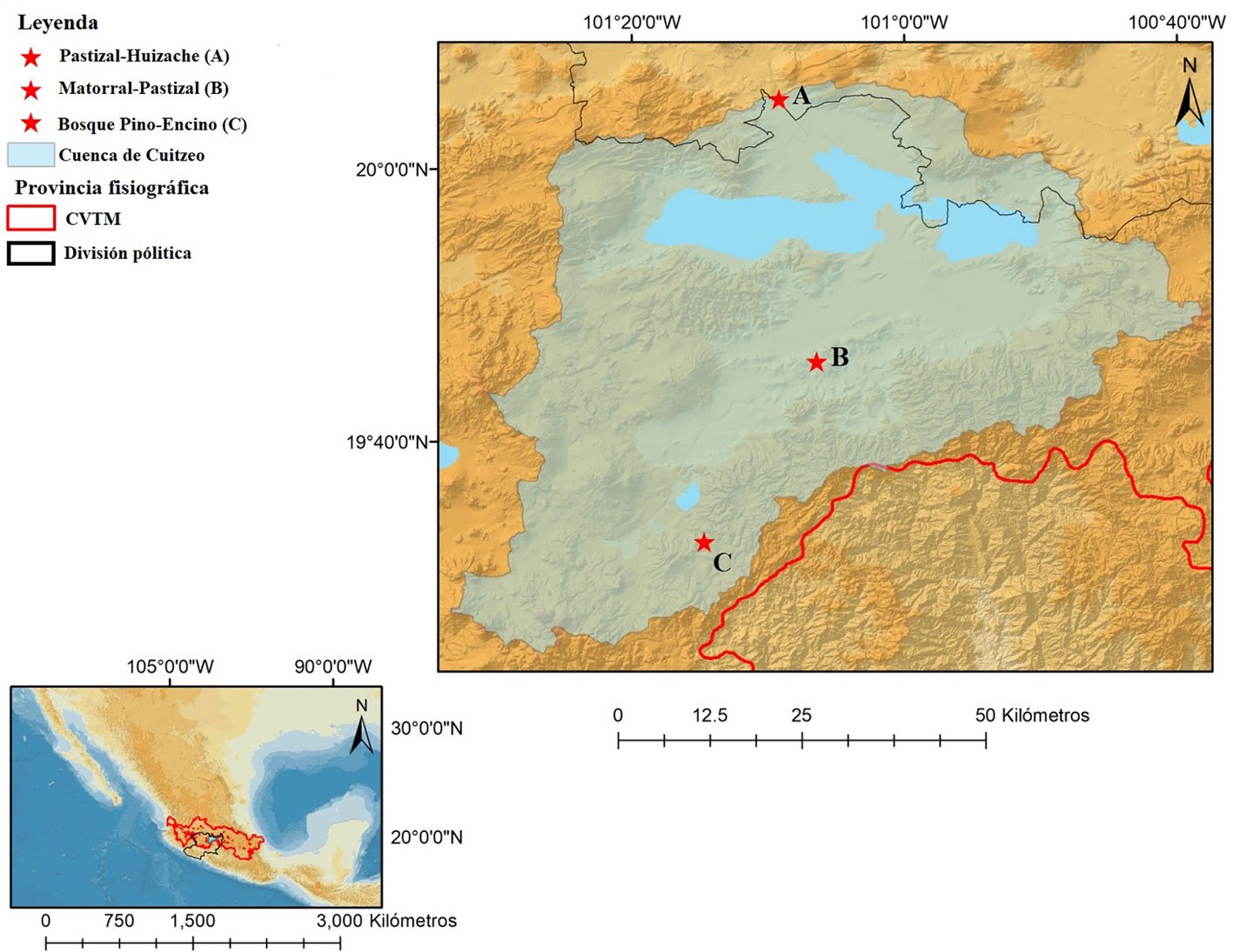
La caracterización de la vegetación se hizo en el estrato herbáceo mediante 5 cuadrantes de 5 m², cada cuadrante con 5 unidades de muestreo de 1 m² (25 unidades en total, por cada sitio y para cada estación), distribuidas en arreglo “5 de oros”, una en el centro y las demás en las esquinas (Senasica, 2024). Se identificaron familias y géneros, y se registró su abundancia y cobertura horizontal en porcentaje. La determinación taxonómica de las plantas se limitó a género debido al estado fenológico de las plantas en algunas estaciones, se utilizó el término morfotipo para las plantas solo identificadas hasta familia.
Para la vegetación se describió la estructura general en los niveles taxonómicos de familia y género para cada sitio y época del año incluyendo composición y abundancias.
Para los roedores se analizó la riqueza y abundancia para cada localidad, época de recolecta y para todo el año. Para evaluar la relación entre la riqueza de especies en función del esfuerzo de muestreo, se elaboraron curvas de rarefacción para cada sitio que permitieron estimar la eficiencia del muestreo utilizando el acumulado por individuos (Chao et al., 2014, 2016). Posteriormente, se estimó la completitud del muestreo a través de las estimaciones no paramétricas de riqueza de Chao 2 y bootstrap. Se elaboraron curvas de rango-abundancia para describir las relaciones de abundancia entre las especies y determinar las dominancias para cada localidad y época del año.
Se calcularon los índices de diversidad de Shannon-Wiener (H´) y dominancia Simpson (D), tanto por sitio de estudio como por temporada. Se utilizó la prueba de t modificada por Hutchenson (1970) para probar las diferencias estadísticas, se incluyó además el cálculo de los límites de confianza (LC) a 95% por el método de percentiles. Para calcular la equitatividad de las especies se usó el índice de equitatividad de Pielou (J). Para conocer el grado de semejanza entre comunidades se usó el índice de similitud de Jaccard para composición de especies y el índice de Bray-Curtis para considerar la abundancia en la comparación (Magurran, 2004).
Con el fin de evaluar posibles diferencias en la composición de especies en relación con los hábitats, se aplicó un análisis de las similitudes entre comunidades (Anosim), con 10,000 permutaciones y disimilitud de Bray-Curtis. Todos los análisis antes mencionados se hicieron con el Software Past 4.12 (Hamer et al., 2001).
Resultados
La comunidad vegetal durante un ciclo anual se caracterizó por presentar 31 familias y 105 géneros de plantas en una muestra de 15,060 individuos del estrato herbáceo, de los que 51% correspondió a la asociación pastizal-huizache. El 39% se registró para matorral-pastizal y 10% en pino-encino.
En la asociación pastizal-huizache predominó la familia Poaceae, con abundancia relativa (AR) de 80% y cobertura horizontal relativa (CH) de 86%. Destacan los géneros Chloris (AR = 44%; CH = 51%), Paspalum (AR = 12%; CH = 3%) y Distichlis (AR = 9%; CH = 22%), esas proporciones fueron constantes durante todo el año. En el estrato arbóreo destaca el huizache (Vachellia sp.).
Tabla 1
Especies registradas y sus abundancias (absoluta y relativa = tasas de captura) en 3 asociaciones vegetales de la cuenca de Cuitzeo en un ciclo de muestreo anual. S = Secas; H = húmedas; PLL = posterior a lluvias; SF = secas frías.
| Especie | Pastizal-huizache (1,838 m snm) | Matorral-pastizal (1,896 m snm) | Pino-encino (2,132 m snm) | Subtotales (tasa de captura) | |||||||||
| Heteromys irroratus | 0 | 2 | 0 | 0 | 0 | 1 | 0 | 7 | 0 | 0 | 0 | 0 | 10 (0.31) |
| Baiomys taylori | 0 | 1 | 0 | 3 | 1 | 1 | 3 | 28 | 0 | 0 | 0 | 0 | 37 (1.16) |
| Baiomys musculus | 1 | 0 | 0 | 0 | 1 | 0 | 0 | 0 | 0 | 0 | 0 | 0 | 2 (0.063) |
| Sigmodon hispidus | 0 | 0 | 0 | 2 | 0 | 0 | 0 | 0 | 0 | 0 | 0 | 0 | 2 (0.063) |
| Sigmodon mascotensis | 0 | 0 | 0 | 1 | 0 | 0 | 0 | 0 | 0 | 0 | 0 | 0 | 1(0.031) |
| Oligoryzomys fulvescens | 0 | 1 | 0 | 0 | 0 | 0 | 0 | 0 | 1 | 0 | 0 | 0 | 2 (0.063) |
| Peromyscus labecula | 0 | 0 | 0 | 0 | 0 | 0 | 0 | 0 | 0 | 0 | 1 | 0 | 1(0.031) |
| Peromyscus melanotis | 0 | 0 | 0 | 0 | 0 | 0 | 0 | 0 | 0 | 0 | 0 | 1 | 1(0.031) |
| Peromyscus difficilis | 0 | 1 | 0 | 0 | 0 | 0 | 0 | 1 | 0 | 1 | 4 | 5 | 12 (0.37) |
| Peromyscus hylocetes | 0 | 0 | 0 | 1 | 0 | 0 | 0 | 0 | 0 | 0 | 0 | 1 | 2 (0.063) |
| Peromyscus kilpatricki | 0 | 0 | 0 | 1 | 0 | 0 | 0 | 0 | 0 | 0 | 0 | 3 | 4 (0.12) |
| Peromyscus pectoralis | 0 | 2 | 0 | 0 | 0 | 0 | 0 | 0 | 0 | 0 | 0 | 0 | 2 (0.063) |
| Peromyscus gratus | 0 | 0 | 0 | 0 | 0 | 0 | 0 | 0 | 0 | 0 | 3 | 1 | 4 (0.12) |
| Peromyscus zamorae | 0 | 0 | 0 | 0 | 0 | 0 | 0 | 0 | 0 | 0 | 2 | 0 | 2 (0.063) |
| Reithrodontomys sumichrasti | 0 | 0 | 0 | 0 | 0 | 0 | 0 | 0 | 1 | 0 | 0 | 5 | 6 (0.18) |
| Reithrodontomys fulvescens | 0 | 0 | 0 | 0 | 0 | 0 | 0 | 1 | 0 | 0 | 1 | 0 | 2 (0.063) |
| Mus musculus | 0 | 3 | 1 | 1 | 2 | 0 | 1 | 0 | 0 | 0 | 0 | 0 | 8 (0.25) |
| Submuestra por sitio (%) | 21 (21.4) | 47 (47.9) | 30 (30.6) | 98 (100%) | |||||||||
| Riqueza de especies por sitio | 11 | 6 | 10 | 17 | |||||||||
| Tasa de captura/área | 1.98 | 4.45 | 2.84 | 3.09 | |||||||||
| Especies exclusivas por sitio | 3 | 0 | 5 | 8 |
Tabla 2
Parámetros de riqueza, abundancia (en paréntesis) y tasa de captura de la comunidad de roedores en 3 asociaciones vegetales en función a la época.
| Secas | Húmedas | Posterior a lluvias | Secas frías | |
| Pastizal-huizache | 1-(1)-0.56 | 6-(10)-4.1 | 1-(1)-0.3 | 6-(9)-2.5 |
| Matorral-pastizal | 3-(4)-2.2 | 2-(2)-0.83 | 2-(4)-1.4 | 4-(37)-10.4 |
| Pino-encino | 2-(2)-1.1 | 1-(1)-0.42 | 5-(11)-3.9 | 6-(16)-4.5 |
| Esfuerzo de muestreo/trampas-noche | 540 | 720 | 840 | 1,068 |
| Especies | 5 | 6 | 7 | 12 |
| Especies exclusivas | 1 | 1 | 2 | 6 |
| Sub muestra estacional (%) | 7 (7.1) | 13 (13.2) | 16 (16.3) | 62 (63.2) |
| Tasas de captura general/estación | 1.30 | 1.81 | 1.90 | 5.81 |
El matorral-pastizal está integrado proporcionalmente por las familias Asteraceae (18%), Poaceae (16%), Fabaceae (14%) y Euphorbiaceae (11%). Difiere del pastizal al presentar variación estacional en la estructura y composición de las plantas en el año. Por ejemplo, en secas Lolium presentó la mayor abundancia y cobertura horizontal (AR = 43%; CH = 32%); en temporada húmeda Marina (AR = 29%; CH = 21%), Euphorbia (AR = 22%; CH = 13%) y Adenophyllum (AR = 20%; CH = 19%); en la temporada posterior a lluvias Simsia (AR = 20%; CH = 20%) y Eragrostis (AR = 16%; CH = 16%), y en secas frías, una especie de gramínea (AR = 42%; CH = 55%), que por su fenología no pudo ser identificada. También se presentaron elementos aislados de Opuntia.
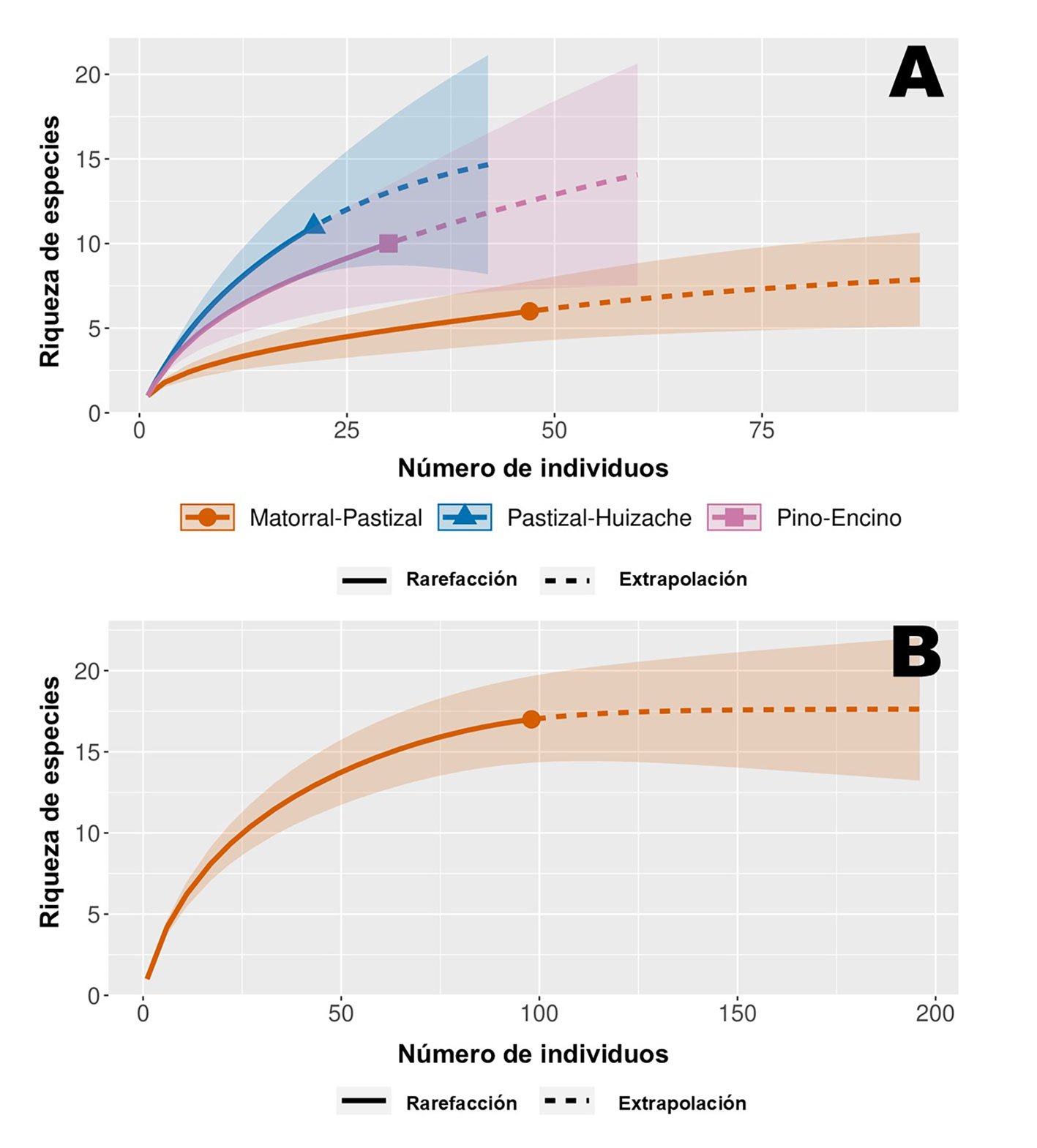
Figura 2. A, Curvas de rarefacción de riqueza de especies en función de las abundancias de roedores en sitios de colecta; B, curva de rarefacción con riqueza de especies en función abundancias de roedores colectadas durante el ciclo anual en los 3 sitios.
La vegetación en el área de pino-encino se caracterizó en el estrato arbóreo por la presencia de Pinus y Quercus. El estrato herbáceo se caracterizó por el predominio de las familias Poaceae, Rosaceae, Asteraceae, Oxiladaceae, Fabaceae, Anacardiaceae, Pteridaceae y Cyperaceae con 78% de la muestra total. El género Rubus (AR = 29%; CH = 13%) predominó en secas, mientras que en húmedas fue Oxalis (AR = 31%; CH = 9%) y Centella (AR = 19%; CH = 17%); en la temporada post-lluvias (AR = 19%; CH = 11%) y secas frías (AR = 27%; CH = 13%) fueron macollos de gramíneas que carecían de espiga por lo que no se identificaron, posiblemente del género Microstegium (apéndice 1).
La muestra de roedores capturados incluyó 98 individuos. Los ejemplares se identificaron como 16 especies nativas y Mus musculus (introducida), pertenecientes a 7 géneros en las familias Cricetidae (15), Heteromyidae (1) y Muridae (1) (tabla 1).
Con base en la curva de rarefacción, se interpreta el esfuerzo de muestreo como suficiente en registrar la riqueza esperada de los 3 sitios; con una cobertura de la muestra de 93% en matorral-pastizal, 83% en el bosque de pino-encino y 72% en pastizal-huizache (fig. 2A). A nivel regional, según los estimadores Chao 2 y bootstrap, la riqueza se espera entre 18-19 especies, solo 2 por encima de la riqueza observada, lo que permite asumir un muestreo de inventario de especies de roedores para la zona suficientemente completo, y que se corrobora con una cobertura de muestra total de 97% en la curva de rarefacción (fig. 2B). Siendo en el pastizal-huizache y en el bosque de pino-encino donde existe mayor oportunidad de registrar otras especies.
La mayor riqueza de especies se observó en el pastizal-huizache, seguido de la asociación de pino-encino y la asociación matorral-pastizal, y en este mismo orden las abundancias se comportaron de menor a mayor (tabla 1; fig. 3A). En relación con la temporada de recolecta, la riqueza y abundancia en secas es en la que se obtuvo la menor cantidad de ejemplares. Posteriormente, se incrementó el éxito de captura para las temporadas siguientes hasta llegar a secas frías (tabla 2); sumando los datos de riqueza y abundancia de las 3 comunidades se observa un incremento en la complejidad (fig. 3B). En las temporadas invernales (secas frías) se destaca la mayor abundancia y tasas de captura de todo el estudio, particularmente en el matorral-pastizal. También se registró la mayor riqueza de especies (n = 12), la mayor abundancia absoluta (62 individuos) y la mayor tasa de captura de 5.8/100 trampas-noche (tabla 2).
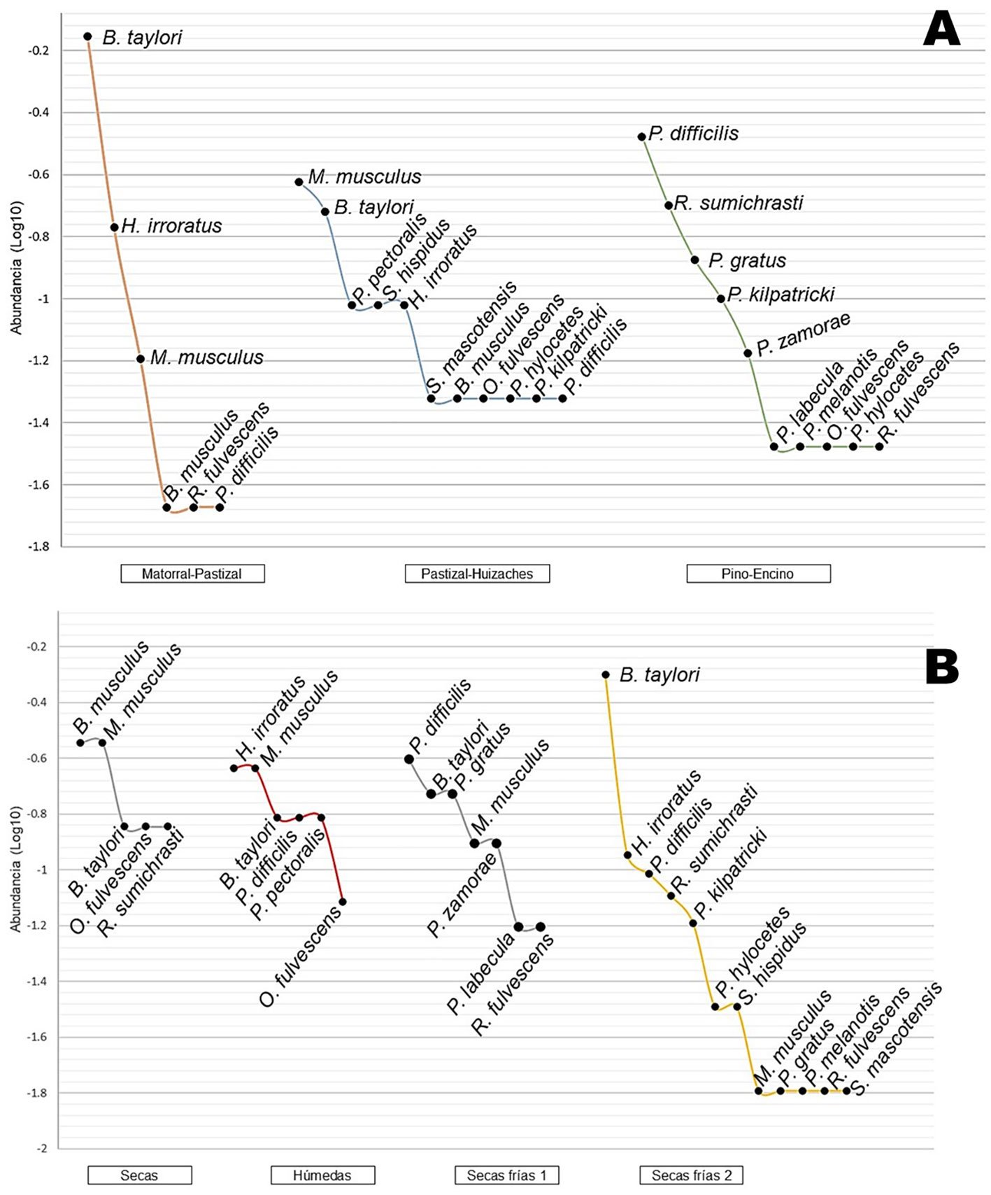
Figura 3. A, Curvas de rango-abundancia entre los sitios de estudio; B, curvas de rango-abundancia entre las temporadas del año de estudio sumando los 3 hábitats.
Baiomys taylori fue la especie más abundante, representó 33% del total de individuos recolectados, con los valores más altos en la temporada de secas frías, se presentó durante todo el año principalmente en matorral-pastizal (n = 33), seguido de pastizal-huizache (n = 4). La especie que resultó con mayor abundancia en el hábitat de pastizal-huizache fue Mus musculus, que también se registró en matorral-pastizal y presente durante todo el año. Para el bosque de pino-encino las especies con más individuos fueron Peromyscus difficilis y Reithrodontomys sumichrasti, la primera se encontró todo el año exceptuando en secas, además destaca por ser la única registrada para las 3 localidades. Por el contrario, las especies Peromyscus labecula, Peromyscus melanotis, y Sigmodon mascotensis, estuvieron representadas por solo 1 individuo; mientras que Baiomys musculus, Oligoryzomys fulvescens, Peromyscus hylocetes, Peromyscus zamorae, Peromyscus pectoralis, Reithrodontomys fulvescens y Sigmodon hispidus contaron con 2 ejemplares, estas especies en conjunto representan 59% de la riqueza total del estudio (fig. 3; tabla 1).
Tabla 3
Valores con el índice de diversidad de Shannon-Wiener (H´), índice dominancia de Simpson (D) e índice de equidad de Pielou (J) para la comunidad de roedores de la cuenca de Cuitzeo. Prueba de t modificada por Hutchenson H´/D para diferencias significativas (*).
| Prueba de t modificada por Hutchenson | ||||||
| H´ | D | J | Matorral-pastizal | Pastizal-huizache | Pino-encino | |
| Matorral-pastizal | 0.97 | 0.52 | 0.54 | D = 3.8822E-05* | D = 0.00042* | |
| Pastizal-huizache | 2.19 | 0.13 | 0.91 | H´ = 3.035E-06* | D = 0.3657 | |
| Pino-encino | 1.93 | 0.18 | 0.84 | H´ = 6.886E-05* | H´ = 0.276 |
Mediante el índice de diversidad de Shannon-Wiener (H´) y la equitatividad de Pielou (J), con límites de confianza (LC) de 95%, se concluye que el hábitat que presentó mayor diversidad y equitatividad en la comunidad de pequeños roedores fue el pastizal-huizache con H´ = 2.19 (LC = 1.69-2.29) y J = 0.91 (LC = 0.81-0.96), en cambio matorral-pastizal fue poco diverso con H´ = 0.97 (LC = 0.66-1.22) y su equitatividad fue las más baja con J = 0.54 (LC = 0.42-0.70); el bosque de pino-encino presento una diversidad de H´ = 1.93 (LC = 1.68-2.13) y J = 0.84 (LC = 0.74-0.92). La prueba de t modificada por Hutchenson no muestra diferencias significativas entre pastizal-huizache y pino-encino, pero sí entre matorral-pastizal con respecto a las otras 2 comunidades. Este efecto también se observa con el cálculo de los límites de confianza en donde solamente en pastizal-huizache y pino-encino existe traslape tanto en H´ como en J. En relación con la temporada de recolecta y como se observa en la tabla 1, en algunos casos solo se capturaron 1 o 2 ejemplares por sitio y temporada, por tanto, conocer la diversidad de los sitios en función de las temporadas no es posible. Aun así, si se toma la sumatoria de los 3 hábitats por época de recolecta se observa poca variación de la diversidad: secas, H´ = 1.55 (LC = 0.79-1.55); húmedas H´ = 1.73 (LC = 1.26-1.73); post lluvias, H´ = 1.84 (LC = 1.35-1.87) y finalmente secas frías, H´ = 1.75 (LC = 1.41-1.99), sin diferencias significativas entre temporadas del año y traslape de los intervalos de confianza en todos los casos.
Por su parte, con el índice de dominancia de Simpson (D) el valor más alto se registró en matorral-pastizal con D = 0.52 y su dominancia con la especie B. taylori es diferente a los otros 2 sitios, en donde no se observaron especies dominantes (tabla 3).
De acuerdo con el índice de similitud de Jaccard para la composición de la comunidad de roedores, el matorral-pastizal y pastizal-huizaches presentan mayor similitud, a diferencia de la comparación entre matorral-pastizal y bosque pino-encino con menor similitud; considerando las abundancias, este patrón se repite según el índice de Bray-Curtis (tabla 4). Con el análisis de similitud entre comunidades (Anosim) se estima diferencias significativas (R = 0.35; p = 0.008) en la composición y abundancia entre los hábitats matorral-pastizal y bosque de pino-encino (p = 0.030) (fig. 4).
Tabla 4
Índice de similitud de Jaccard (ISJ) y Bray-Curtis (BC) para la comunidad de roedores en las 3 asociaciones vegetales examinadas de la cuenca de Cuitzeo.
| Matorral-pastizal | Pastizal-huizache | Pino-encino | |
| Matorral-pastizal | 1 | BC = 0.32 | BC = 0.05 |
| Pastizal-huizache | ISJ = 0.41 | 1 | BC = 0.15 |
| Pino-encino | ISJ = 0.14 | ISJ = 0.23 | 1 |
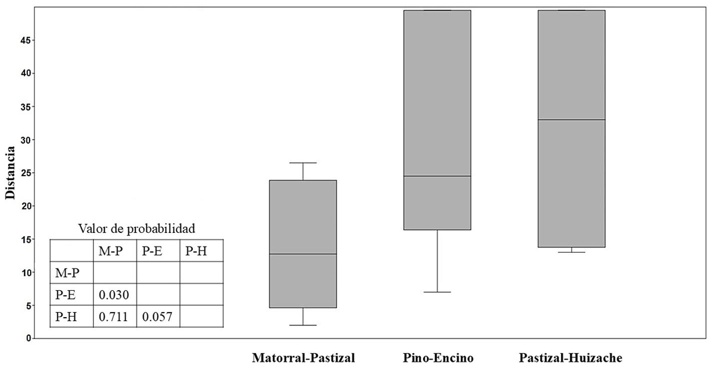
Figura 4. Boxplot y valores de probabilidad del análisis de similitudes (Anosim) entre las 3 asociaciones vegetales para la comunidad de roedores en de la cuenca de Cuitzeo (R = 0.35; p = 0.008). M-P = Matorral-pastizal, P-E = bosque de pino-encino y P-H = pastizal-huizache.
Discusión
Los resultados obtenidos ofrecen 4 aspectos emergentes: riqueza de especies, baja abundancia general, mayores abundancias invernales y baja similitud relativa entre los ambientes muestreados. Recientemente, se evaluó la mastofauna que habita en la cuenca de Cuitzeo. En total se registraron 68 especies de mamíferos, con 28 del orden Rodentia, que representaron 54% de las especies registradas en Michoacán (Monterrubio et al., 2019). Con el presente trabajo se suman al registro de Rodentia para la región a B. musculus, P. pectoralis y O. fulvescens, especies que están presentes en otras áreas del eje Neovolcánico y el bajío (Sánchez et al., 2005), pero que no habían sido registradas para la cuenca. Al incluir estos nuevos registros para la cuenca, en esta zona se presenta 60% de las especies de roedores documentadas para Michoacán (Monterrubio et al., 2014). Otro aspecto notable, es que el esfuerzo de muestreo desarrollado proporcionó el registro del mayor número de especies (16) en cualquier estudio efectuado para la cuenca (Apéndice 2). Esta riqueza sobresale también en el contexto nacional, ya que los intervalos de riqueza específica reportados suelen estar entre 5 y 18 especies (Apéndice 3), generalmente se observan valores bajos en áreas pequeñas y aumentan cuando el estudio es a escala regional.
En contraste, fue sorpresiva la baja abundancia general, con solo 98 registros, en comparación con otros estudios de diferentes regiones del país, en los que con esfuerzos entre 455 y 28,242 noches/trampa se obtienen capturas superiores a 100 individuos (Apéndice 3). Una razón probable de la baja abundancia para la mayoría de especies puede ser la disminución de las precipitaciones en la región. Con base en los datos históricos y comparando con los últimos años, se ha experimentado sequía en algunas partes de la cuenca (Hernández et al., 2023), para lo que probablemente hayan respondido las poblaciones de roedores con menor reproducción o migración. Otra evidencia es la cifra de capturas del muestreo de la temporada de secas frías (fig. 3B) y posterior a la época de lluvia de la cuenca, dado que se registró un incremento notable en el número de capturas, tanto en riqueza específica como en abundancia. Este fenómeno es similar al observado en otros estudios (Flores y Vázquez, 2016; Zaragoza et al., 2022). El aumento poblacional en esta época ocurrió para B. taylori, P. difficilis y H. irroratus; en las primeras 2 especies ya se ha registrado aumento en densidades poblacionales en temporadas frías del año (Eshelman y Cameron, 1987; Fernández et al., 2010), mientras que el aumento de H. irroratus, según antecedentes, se reporta de agosto a noviembre (Dowler y Genoways, 1978).
El índice de diversidad no muestra variación significativa entre épocas del año, esto podría indicar que la diversidad es explicada en mayor medida por el hábitat y que genera niveles importantes de estabilidad reflejada en los valores de equitatividad obtenidos (entre 0.57 y 1), lo cual también sugieren Luévano et al. (2008), particularmente en zonas de matorrales.
Las 3 comunidades de roedores examinadas muestran en general baja similitud, y parece observarse una posible influencia de la estratificación de la vegetación. En general, a mayor complejidad estructural de la vegetación con presencia del estrato arbóreo, se observa mayor riqueza de especies. Este patrón se presentó para el pastizal-huizache y el bosque de pino-encino en donde no existió diferencia significativa de diversidad y tampoco hubo traslape de intervalos de confianza. En cambio, la abundancia de roedores fue mayor en el matorral-pastizal y en el pino-encino, en ambos hábitats se observa mayor riqueza de la vegetación a nivel herbáceo. El patrón de aumento en las abundancias para ambientes de mayor heterogeneidad también lo encontraron Morales et al. (2019) y contrasta con la homogeneidad del estrato herbáceo y baja densidad de roedores registrada para el pastizal-huizache de este estudio. Todavía no es clara la relación entre la estructura de la comunidad de roedores y la conectividad de los hábitats. La dinámica de la cuenca de Cuitzeo implica un aumento de la colonización humana y más actividades agropecuarias en las últimas décadas (Escamilla y Aguilar, 2010). Dicha expansión ha degradado y fragmentado los hábitats originarios, hasta llegar a tener 6% con asentamientos humanos y 50% de la cuenca destinado a zonas de cultivo y pastoreo (INEGI, 2023). Con este panorama, es posible que la estructura y composición de las comunidades de pequeños roedores observada puede deberse al grado de aislamiento diferenciado entre los distintos hábitats. Los pastizales presentan conectividad con los extensos cultivos, permitiendo la cohesión espacial de algunas especies, mientras que las zonas de matorral y arbóreas presentan índices muy bajos de conectividad (Correa et al., 2014). El aislamiento en estos hábitats, principalmente matorrales, puede disminuir a los depredadores, lo que se ve reflejado en el aumento de poblaciones de roedores más generalistas y menor riqueza especifica (Young et al., 2015); este proceso puede estar presente en el sitio de matorral-pastizal. Aunque en el caso de las zonas montañosas de la cuenca con bosques, todavía parece existir mayor conectividad y esta se ve reflejada en la riqueza de la mastofauna (Monterrubio et al., 2019).
El pastizal-huizache se extendía originalmente en forma extensa (López et al., 2010), ahora es un ambiente con elevada fragmentación y es quizás uno de los hábitats más amenazados por el elevado establecimiento de asentamientos humanos y campos de cultivo. Sin embargo, la diversidad de roedores observada en este hábitat parece todavía estar explicada por la vegetación más que por la antropización vecina. Los 3 géneros de plantas herbáceas más representativos de la zona (Chloris, Distichlis y Panicum) son gramíneas no invasivas y componentes de la vegetación original (Herrera y Pámanes, 2010). Peromyscus pectoralis, Sigmodon hispidus y S. mascotensis resultaron exclusivas a esta localidad entre los 3 hábitats estudiados, y parecen coincidir con ambientes en que se han registrado regularmente, que incluyen aridez relativa, pastizales y ambientes rocosos (Baccus et al., 2009; Fleharty y Olson, 1969; Martínez et al., 2017). En hábitats similares la exclusividad reportada suele ser de 1 a 2 especies (Cimé et al., 2010; Elizalde et al., 2014; Hernández et al., 2012), lo cual coincide con lo registrado en este trabajo. Además, la cercanía con sembradíos parece proveer de alimento, lo que facilita la coexistencia entre especies, ya que los roedores también consumen materiales de los cultivos, como se ha documentado en plantaciones de caña (Peña et al., 2009).
Para el matorral-pastizal, la baja diversidad de roedores podría explicarse en parte por la poca conectividad y por la biología de la comunidad vegetal, ya que los géneros más abundantes están asociados con ambientes alterados. En temporada seca el género herbáceo Lolium (Poaceae), especie introducida en México (Herrera y Pámanes, 2010), fue la más abundante y fue en esta temporada cuando se recolectaron pocos roedores (n = 4), 2 de los cuales fueron M. musculus, especie que puede considerarse indicadora de deterioro del hábitat. En relación con las plantas de temporadas restantes del año, son géneros nativos con distribución principalmente en matorrales como Marina (M. cf. nutans) y Adenophyllum, y junto con Euphorbia (E. cf. dentata), Simsia (S. cf. foetida) y Eragrostis (E. cf. intermedia), pero crecen en afinidad a lugares ruderales con tendencia a disturbios (Rzedowski y Rzedowski, 2005). En los recorridos de campo se observaron asentamientos humanos e infraestructura inconclusa, indicativa de la expansión de la mancha urbana, así como fauna doméstica, perros principalmente, caminando en búsqueda de alimento entre la vegetación.
El registro de B. taylori, especie que se conoce con una mayor densidad de individuos distribuyéndose en matorrales y zonas áridas (Packard, 1960), coincidió con el hábitat de recolecta. Este cricétido junto con H. irroratus podrían ilustrar su resiliencia a los ambientes perturbados, tendencia que se ha reportado para mamíferos de tallas pequeñas, particularmente en roedores y murciélagos (Dirzo et al., 2014), aunque también pudiesen ser evidencia de que el hábitat de matorral-pastizal en la región experimenta un proceso de homogeneización de la comunidad de roedores.
Por su parte, el bosque de pino-encino (La Planta) solo se diferencia con el pastizal-huizache por tener una especie menos (la invasora M. musculus); pero en índices cuantitativos la similitud fue baja. Este hábitat, donde cobertura y dominancia de biomasa vegetal corresponden a Pinus y Quercus (Gómez-Tagle et al., 2015), no se recolectaron especies de roedores introducidas. O. fulvescens, R. sumichrasti y las especies del género Peromyscus se reportan en bosques conservados y áreas con corrientes de agua cercanas (Fernández et al., 2010; Spencer y Cameron, 1982), lo cual coincide en lo general con este estudio. Sin embargo, aunque parece un espacio conservado por la estructura de su comunidad de roedores y su flora, también presenta cambio en el uso de suelo en los alrededores, principalmente por expansión del cultivo del aguacate y arándano. Aquí se presentaron 5 especies exclusivas, y coincide con lo registrado en otros estudios en ambientes semejantes en los que la exclusividad de especies va de 1-4 (Flores y Vázquez, 2016; Mendoza y Horváth, 2013; Villanueva, et al., 2017; Zalapa et al., 2012).
Es importante continuar con muestreos con el fin de conocer mejor la dinámica estacional y espacial de las poblaciones de roedores en los distintos ambientes, ya que cada hábitat difiere de nivel de fragmentación y extensión en la cuenca, sobre todo en esta región considerada de importancia para la conservación de la biodiversidad en todos los niveles (Aguilar et al., 2010). Finalmente, en el centro de México desaparecen rápidamente los hábitats naturales, es urgente utilizar la información generada por múltiples inventarios para la priorización y establecimiento de áreas a restaurar y para conservar espacios representativos de todos los hábitats, especialmente donde habitan especies endémicas como lo es Peromyscus ensinki (Bradley et al., 2021). En la cuenca debe estudiarse el grado de tolerancia que especies listadas en categorías de riesgo tienen a la perturbación y como coexisten con especies introducidas, anticipando y examinando los riesgos potenciales de enfermedades zoonóticas, sin olvidar que el bienestar económico no puede lograrse en un entorno sin servicios ambientales y biodiversidad (Villafán et al., 2021; Young et al., 2014).
Referencias
Aguilar, V., Kolb, M., Koleff, P. y Urquiza-Haas, T. (2010). Las cuencas de México y su biodiversidad: una visión integral de las prioridades de conservación. En H. Cotler, A. Garrido, N. Luna, C. Enríquez y M. L. Cuevas (Eds.), Las cuencas hidrográficas de México. Diagnóstico y priorización (pp. 142–151). Ciudad de México: Instituto Nacional de Ecología.
Aragón, E. E., Garza, A. y Cervantes, F. A. (2009). Estructura y organización de los ensambles de roedores de un bosque de la Sierra Madre Occidental, Durango, México. Revista Chilena de Historia Natural, 82, 523–542. http://dx.doi.org/10.4067/S0716-078X2009000400007
Baccus, J. T., Hardwick, J. M., Huffman, D. G. y Kainer, M. A. (2009). Seasonal trophic ecology of the white-ankled mouse, Peromyscus pectoralis (Rodentia: Muridae) in central Texas. Texas Journal of Science, 61, 97–118.
Barragán, F., Lorenzo, C., Morón, A., Briones, M. A. y López, S. (2010). Bat and rodent diversity in a fragmented landscape on the Isthmus of Tehuantepec, Oaxaca, México. Tropical Conservation Science, 3, 1–16. https://doi.org/10.
1177/194008291000300101
Bradley, R. D., Francis, J. Q., Platt, R. N., Soniat, T. J., Álvarez, D. y Lindsey, L. L. (2019). Mitochondrial DNA sequence data indicate evidence for multiple species within Peromyscus maniculatus. Lubbock, TX: Museum of Texas Tech University.
Bradley, R. D., Ordóñez, N., Ceballos, G., Rogers, D. S. y Schmidly, D. J. (2017). A new species in the Peromyscus boylii species group (Cricetidae: Neotominae) from Michoacán, México. Journal of Mammalogy, 98, 154–165. https://doi.org/10.1093/jmammal/gyw160
Bradley, R. D., Ordóñez, N., Thompson, C. W., Wright, E. A., Ceballos, G., Kilpatrick, C. W. et al. (2021). Two new species of Peromyscus (Cricetidae: Neotominae) from the Transverse Volcanic Belt of México. Journal of Mammalogy, 103, 255–274. https://doi.org/10.1093/jmammal/gyab128
Bravo-Espinosa, M., García-Oliva, F., Ríos-Patrón, E., Mendoza-Cantú, M. E., Barrera-Camacho, G., López-Granados, E. et al. (2008). La cuenca del lago de Cuitzeo: problemática, perspectivas y retos hacia su desarrollo sostenible. Morelia Michoacán, México: Consejo Estatal de Ciencia y Tecnología de Michoacán (COECYT). https://doi.org/10.22201/ciga.9789707035782p.2008
Carlón, T. y Mendoza, M. (2007). Análisis hidrometeorológico de las estaciones de la cuenca del lago de Cuitzeo. Investigaciones Geográficas, Boletín del Instituto de Geografía, UNAM, 63, 56–76. https://doi.org/10.14350/rig.29910
Castro, A., Salame, A., Vergara, J., Castillo, A. y Ramírez, J. (2008). Fluctuaciones de micromamíferos terrestres en bosques templados aledaños a la Ciudad de México, Distrito Federal. En C. Lorenzo, E. Espinoza y J. Ortega (Eds.), Avances en el estudio de los mamíferos de México II (pp. 391–410). San Cristóbal de las Casas, Chiapas: Asociación Mexicana de Mastozoología.
Ceballos, G. y Oliva, G. (2005). Los mamíferos silvestres de México. México D.F.: Conabio/ Fondo de Cultura Económica.
Chao, A., Gotelli, N. J., Hsieh, T. C., Sander, E. L., Ma, K. H., Colwell, R. K. et al. (2014). Rarefaction and extrapolation with Hill numbers: a framework for sampling and estimation in species diversity studies. Ecological Monographs, 84, 45–67. https://doi.org/10.1890/13-0133.1al/gyw160
Chao, A., Ma, K. H. y Hsieh, T. C. (2016) iNEXT (iNterpolation and EXTrapolation) Online: Software for interpolation and extrapolation of species diversity. Program and user’s guide. http://chao.stat.nthu.edu.tw/wordpress/software_download/inext-online/
Cimé, J. A., Hernández, S. F., Barrientos, R. C. y Castro, A. A. (2010). Diversidad de pequeños roedores en una selva baja caducifolia del noreste de Yucatán, México. Therya, 1, 23–39. https://doi.org/10.12933/therya-10-2
Correa, C. A., Mendoza, M. E. y López, E. (2014). Análisis del cambio en la conectividad estructural del paisaje (1975-2008) de la cuenca de Cuitzeo, Michoacán, México. Revista de Geografía Norte Grande, 59, 7–23. http://dx.doi.org/10.4067/S0718-34022014000300002
Dirzo, R., Young, H. S., Galetti, M., Ceballos, G., Isaac, N. J. B. y Collen, B. (2014). Defaunation in the Anthropocene. Science, 345, 401–406. https://www.science.org/doi/10.1126/science.1251817
Dowler, R. C. y Genoways, H. H. (1978). Liomys irroratus. Mammalian Species, 82, 1–6. https://doi.org/10.2307/3503813
Elizalde, C., López, J. C., Hernández, L., Laundré, J. W., Cervantes, F. A., Morales-Mejía, F. M. et al. (2014). Registro de presencia y actividades de algunos mamíferos en el Desierto Chihuahuense, México. Therya, 5, 793–816. https://doi.org/10.12933/therya-14-252
Escamilla, I. y Aguilar, G. (2010). Urbanización. En S. Cram, L. Galicia, I. Israde, C. López y B. Ávila (Eds.), Atlas de la cuenca del lago de Cuitzeo: análisis de su geografía y entorno socioambiental (pp. 160–163). México D.F.: UNAM/ UMSNH.
Eshelman, B. D. y Cameron, G. N. (1987). Baiomys taylori. Mammalian Species, 285, 1–7. https://doi.org/10.2307/3503776
Fernández, J. A., García-Campusano, F. y Hafner, M. S. (2010). Peromyscus difficilis (Rodentia: Cricetidae). Mammalian Species, 42, 220–229. https://doi.org/10.1644/867.1
Fleharty, E. D. y Olson, L. E. (1969). Summer food habits of Microtus ochrogaster and Sigmodon hispidus. Journal of Mammalogy, 50, 475–486. https://doi.org/10.2307/1378774
Flores, R. y Vázquez, G. (2016). Influence of vegetation type and season on rodent assemblage in a mexican temperate forest mosaic. Therya, 7, 357–369. https://doi.org/10.12933/therya-16-390
García, U. O. y Flores, O. A. (2010). Biodiversidad: anfibios y reptiles. En S. Cram, L. Galicia, I. Israde, C. López y B. Ávila (Eds.), Atlas de la cuenca del lago de Cuitzeo: análisis de su geografía y entorno socioambiental (pp. 94–95). México D.F.: UNAM/ UMSNH.
García, C., Romero, M. L. y Sánchez C. (2002). Comparison of rodent communities in sites with different degrees of disturbance in deciduous forest of southeastern Morelos, México. Acta Zoológica Mexicana, 85, 153–168. https://doi.org/10.21829/azm.2002.85851819
Gloria-Tapia, G., López, C., González, A. y Hernández, S. F. (2012). Diversidad de roedores y su relación con la heterogeneidad ambiental en la cuenca del río Nazas, Durango, México. En F. A. Cervantes y C. Ballesteros (Eds.), Estudio sobre la biología de roedores silvestres mexicanos (pp. 59–70). México D.F.: Instituto de Biología, UNAM.
Godinez, E. y Guerrero, S. (2014). Los roedores de Jalisco, México: clave de determinación. Therya, 5, 633–678. https://doi.org/10.12933/therya-14-212
Gómez-Tagle, A., Gómez-Tagle, A. F., Ávila, J. A. y Bruijnzeel, L. (2015). Partición de la precipitación en un bosque tropical montano de pino-encino en el centro de México. Bosque, 36, 505–518. https://doi.org/10.4067/S0717-92002015000300017
González, A., Rodríguez, N. V. y Marín, G. (2012). Composición del ensamble de pequeños mamíferos del borde de un bosque mesófilo de montaña en Veracruz, México. En F. A. Cervantes y C. Ballesteros (Eds.), Estudio sobre la biología de roedores silvestres mexicanos (pp. 85–96). México D.F.: Instituto de Biología, UNAM.
Hamer, Q., Harper, D. A. T. y Ryan, P. D. (2001). PasT: Paleontological Statistics Software Package for Education and Data Analysis. Paleontologia Electronica, 4, 1–9.
Hernández, S. F., Cimé, J. A., Medina, S. y Durán C. M. (2012). Parámetros poblacionales del ratón yucateco Peromyscus yucatanicus de una selva baja caducifolia del norte de Yucatán, México. En F. A. Cervantes y C. Ballesteros. (Eds.), Estudio sobre la biología de roedores silvestres mexicanos (pp. 151–164). México D.F.: Instituto de Biología, UNAM
Hernández, L., Laundré, J. W., González, A., López, J. y Grajales, K. M. (2011). Tale of two metrics: density and biomass in a desert rodent community. Journal of Mammalogy, 94, 840–851. https://doi.org/10.1644/10-MAMM-A-175.1
Hernández, A., Ortiz, C. F. y Alcaraz, J. V. (2023). El riesgo agrícola ante el cambio climático en la región de Cuitzeo del estado de Michoacán, México. Acta Universitaria Multidisciplinary Scientific Journal, 33, 1–19. https://doi.org/10.15174/au.2023.3763
Herrera, Y. y Pámanes, D. S. (2010). Guía de pastos de Zacatecas. Durango, Durango, México: IPN/ Conabio.
Hutchenson, K. (1970). A test for comparing diversities base on the Shannon formula. Journal of Theoretical Biology, 29, 151–154.
INEGI (Instituto Nacional de Estadística, Geografía e Informática). (2023). Anuario de estadística por entidad federativa. https://www.inegi.org.mx/contenidos/productos/prod_serv/contenidos/espanol/bvinegi/productos/nueva_estruc/889463906353.pdf
López, C., García, D. F., López, J. C. y Elizalde, C. (2019). Multiple lines of evidence reveal a composite of species in the plateau mouse, Peromyscus melanophrys (Rodentia Cricetidae). Journal of Mammalogy, 100, 1583–1598. https://doi.org/10.1093/jmammal/gyz106
López, E., Mendoza, M. E. y Bocco, G. (2010). Cobertura vegetal y uso del terreno. En S. Cram, L. Galicia, I. Israde, C. López y B. Ávila (Eds.), Atlas de la cuenca del lago de Cuitzeo: análisis de su geografía y entorno socioambiental (pp. 52–57). México D.F.: UNAM/ UMSNH.
Luévano, J., Mellink, E., Riojas, M. E. y Flores, J. L. (2008). Comunidades de roedores nocturnos en un ecotono de matorrales micrófilos y zacatal gipsófilo en San Luis Potosí, México. Revista Mexicana de Biodiversidad, 79, 197–203. https://doi.org/10.22201/ib.20078706e.2008.001.528
Madrigal, X. y Guridi, L. L. (2009). Especies arbóreas en riesgo de la cuenca de Cuitzeo, Michoacán y Guanajuato, México. Morelia: Universidad Michoacana de San Nicolás de Hidalgo.
Magurran, A. E. (2004). Measuring biological diversity. Reino Unido: Blackwell Science Ltd.
Mammal Diversity Database. (2024). Explore current mammalian taxonomy. Recuperado el 16 de junio, 2024 de: https://www.mammaldiversity.org/taxa.html
Martínez, S. T., Schnell, G. D., Sánchez, C. y Romero, M L. (2017). Sigmodon mascotensis (Rodentia: Cricetidae). Mammalian Species, 49, 109–118. https://doi.org/10.1093/mspecies/sex013
Medina, M. y Ortega, J. M. (2010). Biodiversidad: peces. En S. Cram, L. Galicia, I. Israde, C. López y B. Ávila (Eds.),
Atlas de la cuenca del lago de Cuitzeo: análisis de su geografía y entorno socioambiental (pp. 90–93). México D.F.: UNAM/ UMSNH.
Mendoza, V. H. y Horváth, A. (2013). Roedores y murciélagos en la zona cafetalera del volcán Tacaná, Chiapas, México. Therya, 4, 409–423. https://doi.org/10.12933/therya-13-116
Monroy, O., Zarco, M. M., Ramírez, J. y Ulises Aguilera, U. (2011). Diversidad de mamíferos de la Reserva Natural Sierra Nanchititla, México. Revista Mexicana de Biodiversidad, 82, 237–248. https://doi.org/10.22201/ib.20078706e.2011.1.377
Monterrubio, T. C., Charre, J. F., Colín, C. Z. y León, L. (2014). Los mamíferos del estado de Michoacán. Revista Mexicana de Mastozoología Nueva Época, 4, 1–17. https://doi.org/10.22201/ie.20074484e.2014.4.2.193
Monterrubio, T. C., Guido, D., Alanís, L., León, L. y Medellín, J. F. (2019). Mamíferos silvestres de la cuenca de Cuitzeo, México. Acta Universitaria Multidisciplinary Scientific Journal, 29, 1–15. https://doi.org/10.15174/au.2019.1892
Morales, S. P., Álvarez, M. Y., Zamora, M. E., Dirzo, R., Oyama, K. y Ávila, L. D. (2019). Rodent community responses to vegetation and landscape changes in early successional stages of tropical dry forest. Forest Ecology and Management,
433, 633–644. https://doi.org/10.1016/j.foreco.2018.11.037
Núñez, A. y Pastrana, G. (1990). Los roedores michoacanos: manual de identificación. Morelia, Michoacán: Coordinación de la investigación científica, Universidad Michoacana de San Nicolás de Hidalgo.
Packard, R. L. (1960). Speciation an evolution of pygmy mice, genus Baiomys. University of Kansas Publications, Museum of Natural History, 9, 579–670. https://doi.org/10.5962/bhl.part.6498
Peña, J. L., López, J., Alarcón, B., Vargas, M., Vázquez, I. y Landeros, C. (2009). Composición de la dieta de Sigmodon hispidus (Rodentia: Cricetidae) en caña de azúcar. Mastozoología Neotropical, 16, 365–378.
Pérez-Arteaga, A., Gaston, K. J. y Kershaw, M. (2002). Undesignated sites in Mexico qualifying as wetlands of international importance. Biological Conservation, 107, 47–57. https://doi.org/10.1016/S0006-3207(02)00043-5
Pérez, M. y Santos, A. (2010). Movements and capture-recapture data analysis of the vesper rat (Nyctomys sumichrasti: Rodentia, Muridae) in a tropical forest in northeastern Oaxaca, México. Acta Zoológica Mexicana, 26, 627–638. https://doi.org/10.21829/azm.2010.263804
Ponce, J. y Quijano, A. F. (2010). Biodiversidad: insectos y arácnidos. En S. Cram, L. Galicia, I. Israde, C. López y B. Ávila (Eds.), Atlas de la cuenca del lago de Cuitzeo: análisis de su geografía y entorno socioambiental (pp. 82–84). México D.F.: UNAM/ UMSNH.
Ramírez, J., González, N., Gardner, A. L. y Arroyo, J. (2014). List of recent land mammals of México. Lubbock, TX: Museum of Texas Tech University.
Rojas, A., Aguilar, M., Sánchez, C. y Noguera, O. (2012). Uso del espacio y dinámica poblacional del ratón de los volcanes (Neotomodon alstoni) en el Cerro del Ajusco, Distrito Federal, México. En F. A. Cervantes y C. Ballesteros (Eds.), Estudio sobre la biología de roedores silvestres mexicanos (pp. 211–224). México D.F.: Instituto de Biología, UNAM.
Romero, M. L., Sánchez, C., García, C. y Owen, R. (2007). Mamíferos pequeños. Manual de técnicas de captura, preparación preservación y estudio. México D.F.: UNAM.
Ruán, I., Manson, R. H. e Íñiguez, L. I. (2008). Respuesta al borde en poblaciones de pequeños mamíferos en remanentes de bosque mesófilo de montaña del centro de Veracruz. En C. Lorenzo, E. Espinoza y J. Ortega (Eds.), Avances en el estudio de los mamíferos de México II (pp. 511–530). San Cristóbal de las Casas, Chiapas: Asociación Mexicana de Mastozoología.
Rzedowski, G. y Rzedowski, J. (2005). Flora fanerogámica del valle de México. Pátzcuaro, Michoacán: Instituto de Ecología, A.C./ Conabio.
Sánchez, C., García, C. y Romero, M. L. (2005). Distribución y diversidad de roedores del estado de Michoacán, y su asociación con las provincias fisiográficas. En V. Sánchez y R. A. Medellín (Eds). Contribuciones mastozoológicas en homenaje a Bernardo Villa (pp. 451–460). México D.F.: Instituto de Biología; Instituto de Ecología, UNAM/ Conabio.
Semarnat (Secretaría del Medio Ambiente y Recursos Naturales). (2010). Norma Oficial Mexicana NOM-059-SEMARNAT-2010. Protección ambiental – Especies nativas de México de flora y fauna silvestres – Categorías de riesgo y especificaciones para su inclusión, exclusión o cambio – Lista de especies en riesgo. Diario Oficial de la Federación. 30 de diciembre de 2010, Segunda Sección, México.
Senasica (Servicio Nacional de Sanidad, Inocuidad y Calidad Agroalimentaria). (2024). Manual de muestreo programa de vigilancia epidemiológica fitosanitaria. https://www.gob.mx/cms/uploads/attachment/file/895962/MANUAL_DE_MUESTREO_2024.pdf
Sikes, R. S. (2016). 2016 Guidelines of the American Society of Mammalogists for the use of wild mammals in research and education. Journal of Mammalogy, 97, 663–688. https://doi.org/10.1093/jmammal/gyw078
Spencer, S. R. y Cameron, G. N. (1982). Reithrodontomys fulvescens. Mammalian Species, 174, 1–7. https://doi.org/10.2307/3503795
Vázquez, L. B., Medellín, R. A. y Camerón, G. N. (2000). Population and community ecology of small rodents in montane forest of western México. Journal of Mammalogy, 81, 77–85. https://doi.org/10.1644/1545-1542(2000)081<0077:PACEOS>2.0.CO;2
Villafán, K. B., Arellanes, Y., López, R. y Ayala, D. A. (2021). Situación socioambiental en el lago de Cuitzeo, Michoacán (México), desde la responsabilidad social. Economía, Sociedad y Territorio, 21, 599–629. https://doi.org/10.22136/est20211694
Villanueva, A. I., Delgado, D. A., Heynes, S. A., Ruacho, L. y López, C. (2017). Habitat selection by rodents at the transition between the Sierra Madre Occidental and the Mexican Plateau, México. Journal of Mammalogy, 98, 293–301. https://doi.org/10.1093/jmammal/gyw173
Villaseñor-Gómez, L. E. y Villaseñor-Gómez, F. J. (2010). Biodiversidad: avifauna. En S. Cram, L. Galicia, I. Israde, C. López y B. Ávila (Eds.), Atlas de la cuenca del lago de Cuitzeo: análisis de su geografía y entorno socioambiental (pp. 96–99). México D.F.: UNAM/ UMSNH.
Young, H. S., Dirzo, R., Helgen, K. M., McCauley, D. J., Billeter, S. A., Kosoy, M. Y. et al. (2014). Declines in large wildlife increase landscape-level prevalence of rodent-borne disease in Africa. Proceedings of the National Academy of Sciences, 111, 7036–7041. https://doi.org/10.1073/pnas.1404958111
Young, H. S., McCauley, D. J., Dirzo, R., Goheen, J. R., Agwanda, B., Brook, C. et al. (2015). Context-dependent effects of large-wildlife declines on small-mammal communities in central Kenya. Ecological Applications, 25, 348–360. https://doi.org/10.1890/14-0995.1
Zalapa, S. S, Guerrero, S., Badii, M. H. y Cervantes F. A. (2012). Variación espacial del ensamble de pequeños mamíferos de tres áreas de bosque tropical subcaducifolio en la costa norte de Jalisco, México. En F. A. Cervantes y C. Ballesteros (Eds.), Estudio sobre la biología de roedores silvestres mexicanos (pp. 117–126). México D.F.: Instituto de Biología, UNAM.
Zaragoza, E. P., Rodríguez, N. V., Hernández, S. F., León, L. S. y González, M. C. (2022). Abundance, microhabitat and feeding of Peromyscus yucatanicus and Peromyscus mexicanus in the Mexican tropics. Therya, 12, 129–142. https://doi.org/10.12933/therya-22-1189

Distributional patterns of longhorn beetles (Coleoptera: Cerambycidae) in Mexico
Patrones de distribución de cerambícidos (Coleoptera: Cerambycidae) en México
Miguel Ortega-Huerta a, *, Felipe Noguera a, Arcelia Claudina Herrera-Solís b
a Universidad Nacional Autónoma de México, Instituto de Biología, Estación de Biología Chamela, Sede Colima, Carlos de la Madrid Béjar, s/n, Km 1.5, Colonia Centro, 28090 Colima, Colima, Mexico
b Secretaría de Educación Pública, Programa de Telesecundaria, La Selva, 47750 Atotonilco el Alto, Jalisco, Mexico
*Corresponding author: maoh@ib.unam.mx (M. Ortega-Huerta)
Received: 31 December 2025; accepted: 20 August 2025
Abstract
This study constructed a georeferenced database of Cerambycidae species collected in Mexico to document their distributional patterns in the country. A sample of 24 species with a significant number of records was modeled to generate their potential distributions, applying a consensus approach. Four prediction algorithms were used: Maxent, Support Vector Machine, Generalized Linear Model, and Artificial Neural Networks. A total of 1,699 locations were obtained after applying cleaning and georeferencing procedures, resulting in 414 total number of species georeferenced. Species with ≥ 20 records included 9 genera and 24 species with 779 records; species with 5-20 records included 41 genera and 124 species with 1,072 records; species with < 5 records included 94 genera and 266 species with 512 records. Only species with ≥ 20 records were modeled. According to the Maxent algorithm, there were variables with high contribution percentages in predictions. Even though the most frequent values of the environmental (response) variables indicate which areas dominated the species distribution, the range of such values provides an estimate of the span of environmental values where species can occur. Too much taxonomic field work is needed to document the species diversity of Cerambycidae in Mexico.
Keywords: Collection records; Cerambycidae; Species distribution model; Response variable
Resumen
Para este estudio se elaboró una base de datos georreferenciados de especies de Cerambycidae rcolectadas en México para documentar sus patrones de distribución. Una muestra de 24 especies fue modelada para generar sus distribuciones potenciales mediante la aplicación de un enfoque de consenso. Se usaron 4 algoritmos de predicción: Maxent, Support Vector Machine, Generalized Linear Model y Artificial Neural Networks. Un total de 1,699 localidades fueron obtenidas después de aplicar procedimientos de limpiado y georreferenciación, lo que resultó en un total de 414 especies georreferenciadas. Especies con ≥ 20 registros incluyeron 9 géneros y 24 especies con 779 registros; especies con 5-20 registros incluyeron 41 géneros y 124 especies con 1,072 registros; especies con ˂ 5 registros incluyeron 94 géneros y 266 especies con 512 registros. Solamente las especies con ≥ 20 registros fueron modeladas. De acuerdo con el algoritmo Maxent, existieron variables con altos porcentajes de contribución en las predicciones. Los valores más frecuentes de las variables ambientales (respuesta) indicaron cuáles dominaron la distribución de especies y el rango de tales variables provee un estimado de la amplitud de valores ambientales, donde las especies pueden estar presentes. Hace falta mucho trabajo taxonómico de campo para documentar la diversidad de especies de Cerambycidae en México.
Palabras clave: Registros de colectas; Cerambycidae; Modelo de distribución; Variable de repuesta
Introduction
The family Cerambycidae (longhorn beetles) is one of the largest groups of the order Coleoptera, with approximately 35,000 described species, most of which are tropical or equatorial (Monné, 2005; Nearns et al., 2017). About 9,000 species have been described from Alaska to Argentina, and 1,621 species are recorded in Mexico (Bezark & Monné, 2023; Noguera, 2014). The species diversity in Mexico represents 18% of the American fauna and 4.6% of the global fauna (Noguera, 2014). Climate, host plant availability and food resources are the main factors determining Cerambycidae species’ occurrence. Species distribution and biogeographic information is limited, focused mainly on describing these fauna’s origin and lineage (Toledo & Corona, 2006). The main habitat types for Cerambycidae species in Mexico include tropical dry forest, pine, pine-oak, and oak forests, as well as tropical evergreen forest.
The diversity of Cerambycidae is reflected in their color, body shape, and morphology of adults; these have a body size between ± 2.5 mm (Cyrtinus sp.) to over 17 cm (Titanus giganteus). Some species mimic ants (tribes Clytini and Tillomorphini), bees, wasps (Rhinotragini), and beetles (Lycid, Pteroplatini). Larvae are xylophagous and phytophagous, so they play an important role in helping decompose dead and nearly dead trees (Linsley, 1961).
When the 3 dimensions (identity, space, and time) included in biological inventories are integrated with spatial environmental data, it is possible to study a wide range of themes, such as ecology, evolution, and applications in agriculture and human health (Graham et al., 2004). Moreover, the use of information contained in scientific collections is considered fundamental in biogeographic research (Anderson & Martínez-Meyer, 2004).
Advances in statistical techniques, numerical analysis, machine learning algorithms, and geographic information systems (GIS) have been responsible for a significant increase in the elaboration and application of predicted species distribution models over the last few decades (Guisan & Zimmermann, 2000). The application of prediction algorithms and GIS makes it possible to obtain the probability of species presence in locations where there is a lack of species distribution information. This has been particularly useful in domains of ecosystem conservation and management, where it has been possible to identify and protect areas with high biological diversity, notwithstanding the lack or limited data for groups of species (Lobo et al., 2002; Zaniewski et al., 2002). Species distribution modeling is considered an interface between ecological theory and statistical modeling (Austin, 2002).
Many species distribution algorithms have been developed, which aim to improve the prediction of such models (Franklin, 2010). Considering the wide variety of prediction algorithms (Elith & Graham, 2009), a consensus of models has been adopted as an approach to generate more robust species distribution predictions (Araújo & New, 2007). Species distribution algorithms differ in various ways: selection of relevant prediction variables and their response behavior, definition of a fitted function for each variable, weighting of each variable contribution, possibility of prediction variables interaction, and prediction of geographic species occurrence patterns (Elith et al., 2006).
However, one of the main problems in obtaining species distribution predictions is that taxonomic studies of species are incomplete and lack uniformity across different regions. In fact, new species are discovered and recorded frequently (Lobo et al., 2002). Models have been developed that relate species distributions to climate variables for a wide range of taxonomic groups, including plants, insects, mammals, birds, reptiles, and amphibians, allowing for their comparative performance (Huntley et al., 2004). Even though there are many examples of modeling insect species distribution (e.g., Buse et al., 2007; Ballesteros-Mejia et al., 2013, 2017; Barredo et al., 2015; Crawford & Hoagland, 2010; D’Amen et al., 2015; Eickermann et al., 2023; Hassall, 2012; Jung et al., 2016; Lobo, 2016; Ma & Ma, 2023; Senay & Womer, 2019; Silva et al., 2016; Ulrichs & Hopper, 2008; Urbani et al., 2017; Watts & Worner, 2008), other taxonomic groups are preferred nevertheless the higher species diversity of the former.
This study’s main objective is to assemble a database of Cerambycidae species occurrence in the different natural regions of Mexico, based on the information included in biological inventories. Moreover, the study will generate potential habitat distribution models of Cerambycidae species with a significant number of occurrence data.
Materials and methods
The database of sites where Cerambycidae species occur was constructed by retrieving information from recent taxonomic studies. The database also included the results of surveys carried out since 1995, as part of the project Insecta of Tropical Dry Forest in Mexico. Priority information for building the database consisted of species’ taxonomic identity and location data. Biota v2.02 (Colwell, 1996) was the database management system used to store and organize the species information retrieved from both scientific literature and surveys conducted in Mexico’s various natural regions.
Species and locality information were retrieved from taxonomic studies by a group of 5 biology students. Due to logistical constraints, the database was divided into 2 subsets. Subset 1 comprised 5,473 records representing 170 species, which were located in 882 localities (190 locations were georeferenced). Subset 2 contained 5,052 records belonging to 268 species located in 1,093 localities (222 locations were geo-referenced).
The retrieved records included a species taxonomic hierarchy, which was scrubbed to eliminate duplicate records. In total, 1,945 localities were recorded with only 412 geo-referenced. Therefore, georeferencing location information was conducted using: ArcView (v3.2) and ArcMap (v10.0) geographic information systems; geographic data such as roads, localities, and political regionalization provided by INEGI and Conabio, Mexican government agencies; Gazetteers such as GEOLocate, JRC Fuzzy Gazetteer, Biogeomancer, INEGI’s geographic names; MaNIS/HerpNet/ORNIS Coordinate Calculator; Google Map and Geogle Earth.
Species distribution models were generated from those species with ≥ 20 records, which was only a small percentage (6%) of the total species georeferenced (414 species). Species presence records were imported into ArcMap, ensuring that no duplicates or misplaced sites, such as those located in the sea, were included.
Nineteen bioclimatic variables (Supplementary material: A1) were obtained from the WorldClim project (Fick & Hijmans, 2017; https://www.worldclim.org/data/worldclim21.html) while topographic variables (Supplementary material: A1) were obtained from the Hydro 1k dataset (https://www.usgs.gov/centers/eros/science/usgs-eros-archive-digital-elevation-hydro1k).
The bioclimatic variables were generated by interpolating monthly climate data obtained from meteorological stations between 1950 and 2000 (Hijmans et al., 2005). Based on the existing correlation among bioclimatic variables, a subset of variables was selected, avoiding correlations greater than 0.800 between variable pairs. Both the bioclimatic and topographic variables had a 1 × 1 km spatial resolution.
This study generated distribution models based on the application of a consensus approach throughout obtaining the median of 4 algorithms: Maximum Entropy (Maxent), Support Vector Machine (SVM), Generalized Linear Model (GLM), and Artificial Neural Networks (ANN). Maxent was applied independently (Phillips & Dudik, 2008) while the other 3 algorithms were applied by using the Modeco software (Guo & Liu, 2010).
Maxent is a general-purpose machine learning method with a simple and precise mathematical formulation (Phillips et al., 2006). Maxent estimates the distribution (geographic range) of a species by finding the distribution that has maximum entropy (i.e., it is closest to the geographically uniform or most spread out) subject to constraints derived from environmental conditions at recorded occurrence locations (Phillips et al., 2017). Maxent is a general approach for presence-only modeling of species distributions (Phillips et al., 2006). Main parameters applied to generate Maxent models included: hinge, linear, and quadratic were the feature types used; 30% of samples were used for model validation; 3.0 was the regularization multiplier.
The SVM are statistically based models rather than loose analogies with natural learning systems (Guo et al., 2005). SVM are not based on characteristics of statistical distributions so there is no theoretical requirement for observed data to be independent, overcoming the problem of autocorrelated observations. However, model performance will be affected by how well the observed data represent the range of environmental variables (Drake et al., 2006). Even though SVM are designed for positive and negative objects, normally negative data is not available and therefore we have a one-class dataset, which requires the separation of a target class from the rest of the feature space (Guo et al., 2005). Schölkopf (2001) developed an SVM of one class.
SVM uses a functional relationship named kernel to map data onto a new hyperspace in which complicated patterns can be more simply represented (Müller et al., 2001). SVM consists of projecting vectors into a high-dimensional feature space by means of a kernel, which makes possible the fitting of the optimal hyperplane that separates classes using an optimization function (Pouteau et al., 2012). The main SVM parameters are: SVM type = C-SVC; Kernel = radial basis function; degree = 3; gamma = 0.5; cost = 1.
The variants of GLM are widely applied to generate species distribution models (Norberg et at., 2019). GLM is a linear regression method where a predictor is selected to be included or dropped from the considered set of predictors based on a predefined simplification method to minimize overfitting (Catalano et al., 2023). GLM use parametric functions such as linear or higher-degree polynomials to model the relationship between the response and predictive variables (Valavi et al., 2022). A link function transforms the scale of the dependent variable, then a GLM is able to relax the distribution and constancy of variances assumptions that are commonly required by traditional linear models (Guo & Liu, 2010). The GLM is commonly used to model dependent variables that are discrete distributions and are nonlinearly related to independent variables (Guisan et al., 2002). Logit was the link function to run the GLM.
ANNs extract linear combinations of the input variables as derived features and model the output as a nonlinear function of these derived features (Hastie et al., 2001). ANN utilizes intermediate nodes in what is referred to as a “hidden layer”, where each node contributes differentially with respect to the variables included in the model (Williams et al., 2009). ANN provides a flexible generalization of GLM and performs better than the latter when modelling nonlinear relationships (Lek et al., 1966). The BP-ANN parameters were, momentum = 0.3 and learning rate = 0.1
Compounded models were validated by applying the partial ROC test (Peterson et al., 2008). Partial ROC calculation has been proposed because of several advantages: it removes the emphasis on absence data, emphasizes the role of omission error when evaluating niche model predictivity and analyzes limited sector of the ROC space which are not directly relevant (Peterson et al., 2008). The NicheToolBox application (https://luismurao.github.io/GSoC/ntb_tutorial.html) was used to calculate the partial ROC statistics.
A portion of 30% of the total species presence samples was separated to be used as independent samples for model validation. The partial ROC test was run through 500 iterations to calculate the average of ROC statistics. After obtaining consensus distribution models, these were converted to binary models using a threshold of 0.50 across species for cross tabulating the response variables and to generate a richness model. The presence (≥ 0.5)/ absence (< 0.50) for the 24 species were summed to obtain a version of the richness model.
Results
A total of 1,699 locations with complete data were obtained after applying cleaning and georeferencing procedures; however, 246 locations lacked complete geographic information. The total number of species georeferenced was 414 (Supplementary material: A2). Most of data consisted of species with < 20 records (see Supplementary material: A2): species with ≥ 20 records included 9 genus and 24 species with 779 total records; species with 5-20 records included 41 genus and 124 species with 1,072 total records; species with < 5 records included 94 genus and 266 species with 512 total records (Fig. 1).
The groups of species with ≥ 20 and 5-19 records are distributed mostly on the Pacific slope within the states of Oaxaca and Jalisco (Table 1). On the other hand, states like Aguascalientes, Coahuila, México City, and Tabasco included only 1 species. In relation to the country’s natural regions, most records with the highest species presence were found in the tropical dry forest ecoregions (Fig. 2).
In the case of the ≥ 20 group, the tropical forests included twice as many records (348) than the temperate forests (140 records). Despite such a difference, temperate forests showed only 2 fewer species (21 species) than the tropical dry forests (23 species). In the group 5-19 records per species, the differences in record numbers were more accentuated: tropical dry forests included 3 times records (543 for 114 species) than the temperate forests (174 for 63 species). Three natural regions for this group (5-19 records) included a similar number of records: semi-desert (170 records), temperate forests (174 records), and tropical rainforests (172 records). Finally, in this group (5-19 records), the mangrove biome included almost one record per species, 27 and 22, respectively.
Based on the correlation matrix among the prediction variables, the number of variables was reduced from 19 bioclimatic and 3 topographic to 9 and 3, respectively. All selected variables (Table 2) had correlation indexes < 0.80. Figure 3 and Table 3 show the contribution of each variable to the generation of distribution models by the Maxent algorithm.
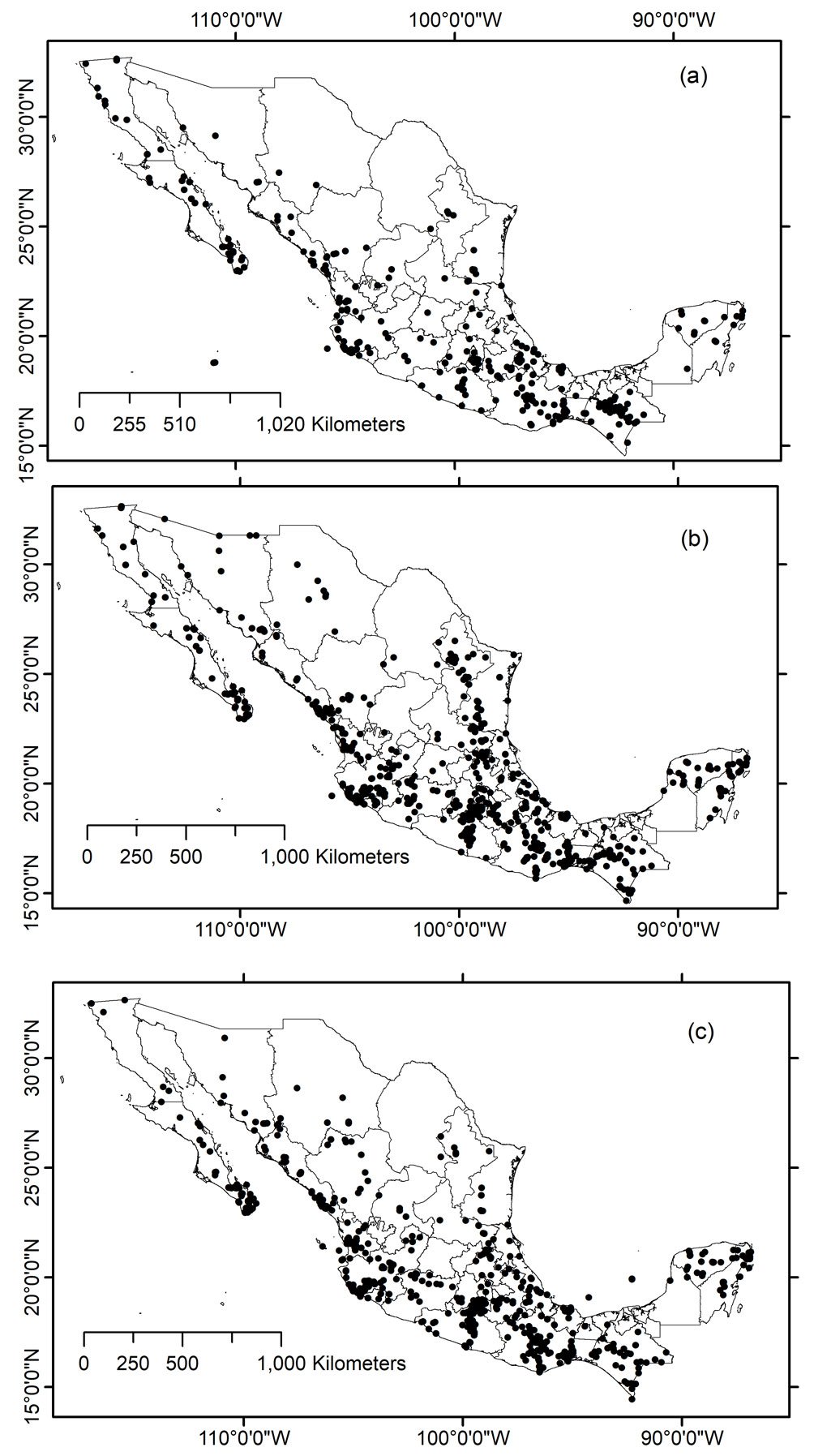
Table 1
Number of Cerambycidae species by state in Mexico.
| State | Species |
| Baja California | 38 |
| Baja California Sur | 62 |
| Campeche | 8 |
| Chiapas | 92 |
| Chihuahua | 8 |
| Coahuila | 4 |
| Colima | 22 |
| Mexico City | 3 |
| Durango | 15 |
| Guanajuato | 2 |
| Guerrero | 67 |
| Hidalgo | 14 |
| Jalisco | 96 |
| Estado de México | 25 |
| Michoacan | 27 |
| Morelos | 45 |
| Nayarit | 49 |
| Nuevo Leon | 17 |
| Oaxaca | 104 |
| Puebla | 36 |
| Queretaro | 3 |
| Quintana Roo | 30 |
| San Luis Potosi | 24 |
| Sinaloa | 47 |
| Sonora | 16 |
| Tabasco | 3 |
| Tamaulipas | 22 |
| Tlaxcala | 1 |
| Veracruz | 66 |
| Yucatan | 33 |
| Zacatecas | 7 |
According to the maxent modelling, some variables showed almost the total contribution percentage in model prediction: For instance, the precipitation of driest month (wc_bio14) had 94% contribution in predicting Phaea acromela and 87% contribution in predicting Eburia brevispinis potential distributions. Similarly, precipitation seasonality (wc_bio15) contributed 79% and 76% for modeling Neocompsa puncticollis asperula and Psyrassa cylindricollis potential distributions, respectively. Other high contribution percentages included: precipitation of wettest month (wc_bio13) had 73% contribution predicting Lagocheirus binumeratus; wc_bio15 had 71% contribution predicting Neocompsa alacris; temperature annual range (wc_bio7) had 71% contribution predicting Lagocheirus araneiformis ypsilon; isothermality (wc_bio3) had 70% contribution predicting Tetraopes umbonatus; wc_bio14 had 61% contribution predicting Lagocheirus procerus; and elevation had 60% contribution predicting Tetraopes femoratus.

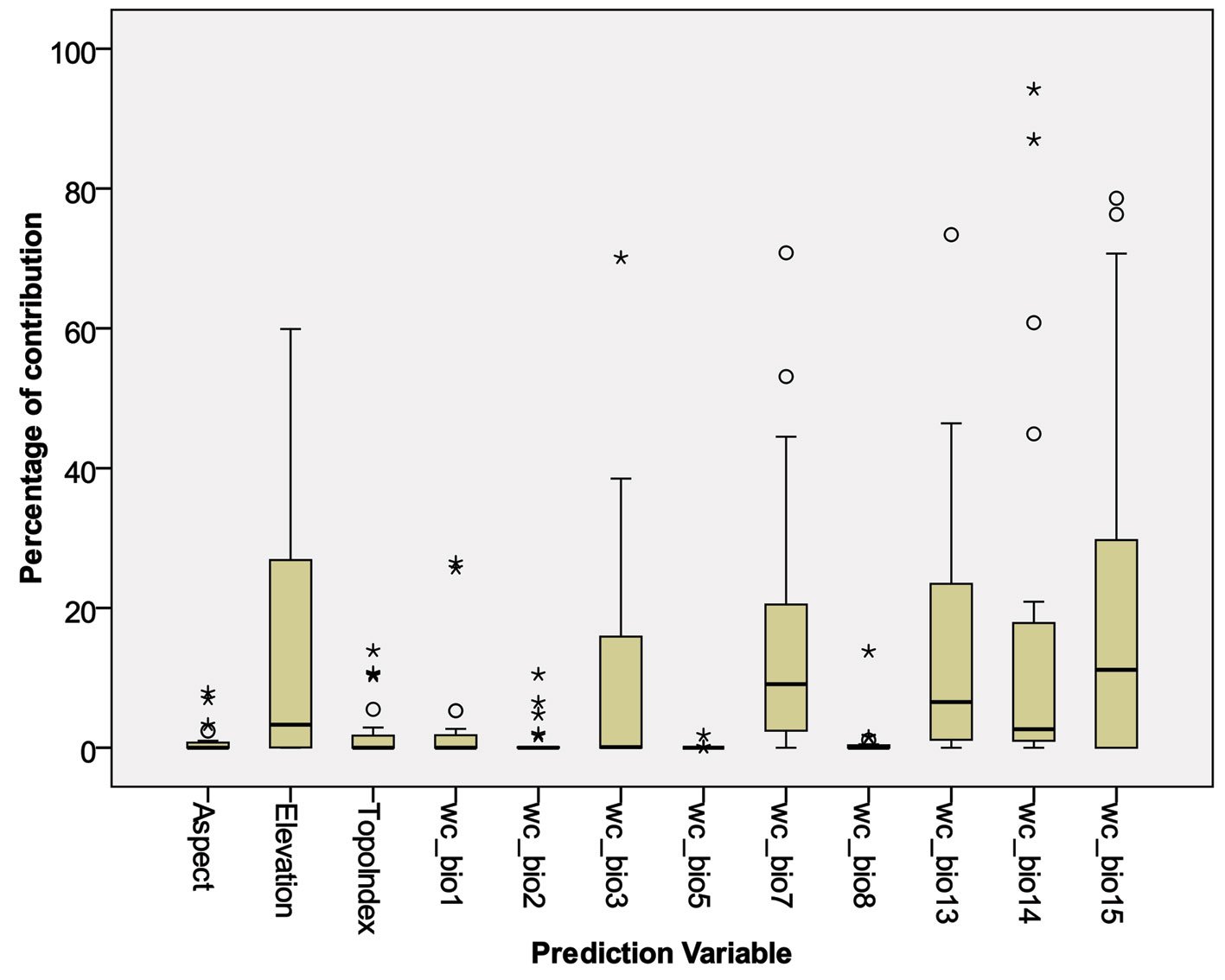
Table 2
Selected prediction variables.
| Bioclimatic variables | |
| wc_bio1 = Annual Mean Temperature | |
| wc_bio2 = Mean Diurnal Range (Mean of monthly [max temp – min temp]) | |
| wc_bio3 = Isothermality (BIO2/BIO7) (×100) | |
| wc_bio5 = Max Temperature of Warmest Month | |
| wc_bio7 = Temperature Annual Range (BIO5-BIO6) | |
| wc_bio8 = Mean Temperature of Wettest Quarter | |
| wc_bio13 = Precipitation of Wettest Month | |
| wc_bio14 = Precipitation of Driest Month | |
| wc_bio15 = Precipitation Seasonality (Coefficient of Variation) | |
| Topographic variables | |
| Elevation | |
| Aspect | |
| Topographic Index |
Considering prediction variables with high contribution percentages for multiple species models, Figure 3 and Table 3 show the most important variables: wc_bio15 (mean = 19%), wc_bio14 (mean = 17%), wc_bio7 (mean = 16%), wc_bio13 (mean = 15%), elevation (mean = 14%), and wc_bio3 (mean = 10%). On the other hand, those prediction variables that had low contribution percentages for fewer species included: Max temperature of warmest month (wc_bio5, mean = 0.09%), mean temperature of wettest quarter (wc_bio8, mean = 0.80%), aspect (mean = 1.06%), mean diurnal range (wc_bio2, mean = 1.07%), topoindex (mean = 2.3%), annual mean temperature (wc_bio1, mean=2.9).
The 4 prediction algorithms, Maximum Entropy (Maxent), Support Vector Machine (SVM), Generalized Linear Model (GLM), and Artificial Neural Networks (ANN) were applied to each of the 24 species that have ≥ 20 records. The models obtained consisted of probability approximations generated by both Modeco and Maxent (ClogLog). The different models for each species were combined by calculating the median value. Then, model accuracy was obtained by calculating the partial ROC test with 500 simulations. These results are shown in Table 4.
In general, the modeled species exhibited high mean AUC ratios and high mean partial AUC values, indicating good model performance, as values of 2.0 and 1.0, respectively, represent a perfect model fit. Mean AUC ratios varied between 1.51 and 1.97, and partial AUC values varied between 0.75 and 0.98. Species with very high mean AUC ratios (> 1.9) included Lagocheirus binumeratus, Psyrassa cylindricollis, Psyrassa sthenias, Neocompsa alacris, Eburia nigrovittata, Euderces batesi. On the other hand, the species with the lowest mean AUC ratios (> 1.5 and < 1.7) were Susuacanga ulkei, Dylobolus rotundicollis, and Tetraopes discoideus.
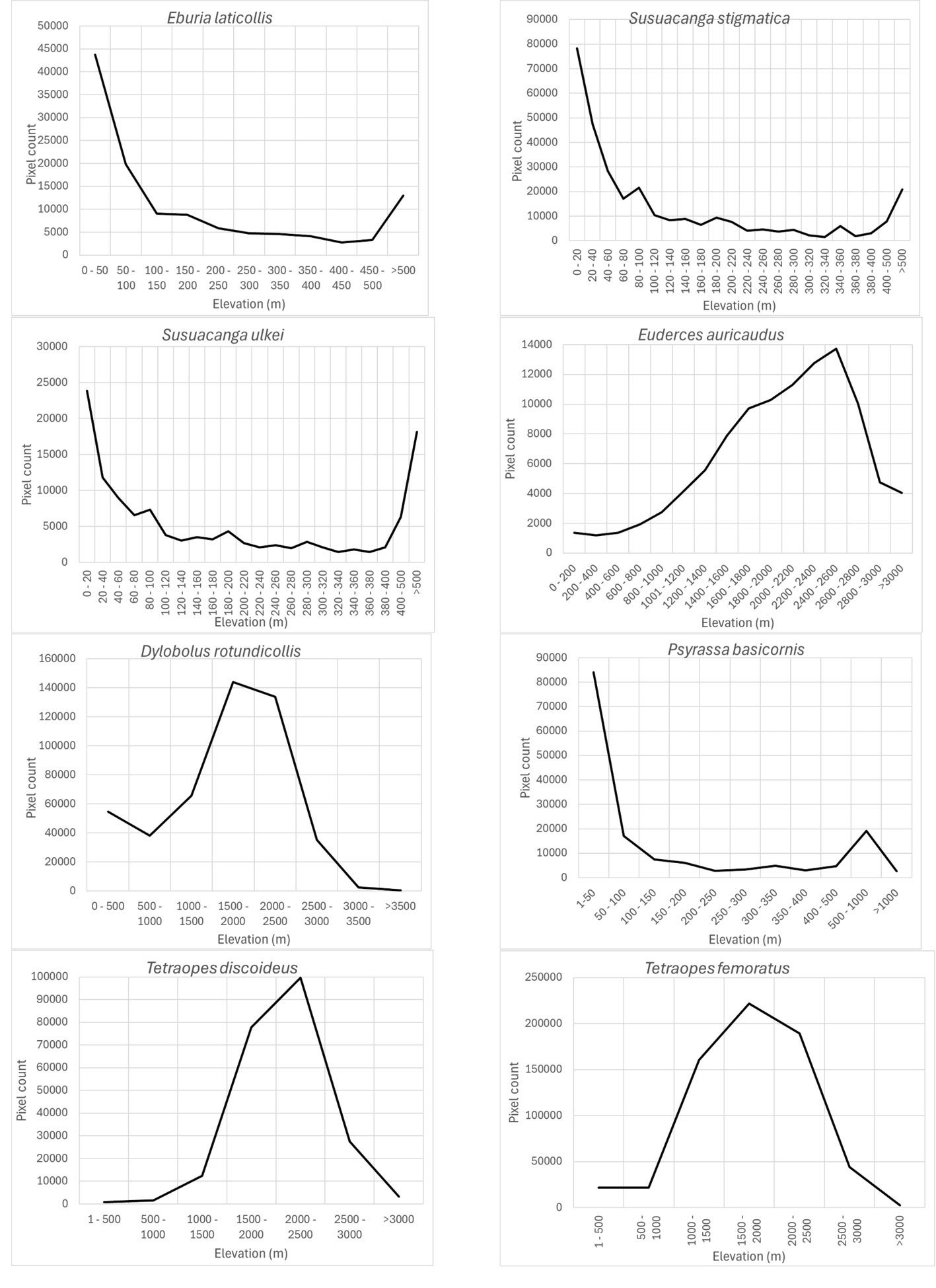
Based on the most important prediction variables identified by the Maxent algorithm, the response variables corresponding to each species model are shown in figures 4-9. For the elevation variable, there were species that preferred elevations between 0 and 50 m: Eburia laticollis, Susuacanga stigmatica, Psyrassa basicornis, and Susuacanga ulkei, which also showed significant predicted areas with elevations above 500 m. On the other hand, there were species selecting distribution areas at much higher elevations: Dylobolus rotundicollis and Tetraopes femoratus at 1,500-2,000 m, Tetraopes discoideus at 2,000-2,500 m, and Euderces auricaudus at 2,400-2,600 m (Fig. 4).
Isothermality (wc_bio3), which is an indicator of daily temperature variation with respect to annual temperature variation, had preferred values < 100 for species models built with this variable as important (35-70%): Highest preferred isothermality values were similar for different species models: Phaea tenuata (65), Euderces batesi (69), Tetraopes umbonatus (70), and Psyrassa sthenias (71) (Fig. 5).
According to Maxent, temperature annual ranges (wc_bio7) were also an important prediction variable for species with different preferring values: 3 species models (Susuacanga stigmatica, Lagocheirus araneiformis, and Psyrassa basicornis) showed temperature annual ranges preferred at 170-180 mm, while Psyrassa sthenias preferred the 18-19ᵒC range. Other species models showed preference for higher temperature annual ranges (Fig. 6): Euderces auricaudus (21-22 ᵒC), Sphaenothecus trilineatus (23-24 ᵒC) and Dylobolus rotundicollis (24-25 ᵒC).
Precipitation of the wettest month (wc_bio13) was another important prediction variable whose highest preferred values varied according to different species: Lagocheirus araneiformis, Dylobolus rotundicollis, Sphaenothecus trilineatus, and Tetraopes discoideus at 150-200 mm; Lagocheirus obsoletus, Mecas obereoides, Phaea tenuata at 200-250 mm; and Lagocheirus binumeratus at 300-350 mm (Fig. 7).
Table 3
Percentage of contribution of each variable in the elaboration of distribution models by the Maxtent algorithm.
| Species | aspect | elevation | topoindex | wc_bio1 | wc_bio2 | wc_bio3 | wc_bio5 | wc_bio7 | wc_bio8 | wc_bio13 | wc_bio14 | wc_bio15 |
| Eburia brevispinis | 0.5 | 0 | 0 | 0 | 4.8 | 0 | 0 | 7.8 | 0 | 0 | 87 | 0 |
| E. laticollis | 0 | 27.4 | 0 | 25.7 | 0 | 0 | 0 | 1.9 | 0 | 0.3 | 11.3 | 33.4 |
| E. nigrovittata | 0 | 0 | 0 | 26.5 | 0 | 0 | 0 | 10.4 | 0 | 2 | 13.5 | 47.6 |
| Susuacanga stigmatica | 0 | 50.2 | 0 | 2.7 | 0 | 0 | 0 | 35.9 | 1.5 | 9.8 | 0 | 0 |
| S. ulkei | 0.1 | 25.8 | 0 | 0 | 0.1 | 2.2 | 0 | 0 | 13.8 | 0 | 44.9 | 13.2 |
| Euderces auricaudus | 0 | 30.7 | 0 | 0 | 0 | 15.3 | 0 | 53.1 | 0.5 | 0 | 0.4 | 0 |
| E. batesi | 0.5 | 24.2 | 0 | 0 | 0 | 35.1 | 1.8 | 19.8 | 0.3 | 15.4 | 3 | 0 |
| Lagocheirus araneiformis ypsilon | 0.3 | 0.1 | 5.5 | 0 | 1.7 | 0 | 0.1 | 70.8 | 0 | 21.1 | 0 | 0.4 |
| L. binumeratus | 7.9 | 0.7 | 0 | 0 | 0 | 0.3 | 0.1 | 17.5 | 0 | 73.4 | 0 | 0 |
| L. obsoletus | 0 | 1.2 | 2.9 | 1 | 0 | 6.1 | 0 | 15.3 | 0 | 46.4 | 16.2 | 10.9 |
| L. procerus | 0 | 4.7 | 0 | 1.4 | 6.5 | 0 | 0 | 1.8 | 0.4 | 13.1 | 60.8 | 11.4 |
| Mecas obereoides | 0 | 0 | 0 | 2.2 | 0 | 0 | 0 | 15.3 | 0 | 37.3 | 1.6 | 43.5 |
| Dylobolus rotundicollis | 0 | 27.1 | 10.3 | 0 | 0 | 0 | 0 | 20.3 | 1.1 | 22.6 | 18.5 | 0 |
| Neocompsa alacris | 0 | 1.9 | 10.7 | 5.3 | 0 | 0 | 0 | 5.6 | 0 | 3.6 | 2.1 | 70.7 |
| N. puncticollis asperula | 7 | 0 | 0 | 0 | 2 | 0 | 0 | 4.7 | 0 | 3.3 | 4.4 | 78.6 |
| Phaea acromela | 3.3 | 0 | 0 | 0 | 0 | 0.2 | 0 | 0 | 0 | 2.4 | 94.2 | 0 |
| P. tenuata | 2.4 | 6.3 | 0.5 | 0 | 0 | 38.5 | 0 | 3.4 | 0 | 43.4 | 2 | 3.5 |
| Psyrassa basicornis | 0 | 26.6 | 0 | 5.3 | 0.1 | 16.5 | 0 | 44.5 | 1.6 | 5.3 | 0.1 | 0 |
| P. cylindricollis | 1 | 9 | 0.6 | 0 | 0 | 0 | 0.1 | 3 | 0 | 7.8 | 2.1 | 76.3 |
| P. sthenias | 2.4 | 0.6 | 0 | 0 | 0 | 35.5 | 0 | 20.7 | 0 | 4.5 | 17.2 | 19.1 |
| Sphaenothecus trilineatus | 0 | 0 | 0.4 | 0.2 | 0 | 14.4 | 0 | 27 | 0 | 25.1 | 20.9 | 12 |
| Tetraopes discoideus | 0 | 41.2 | 10.5 | 0 | 0 | 16.5 | 0 | 1.2 | 0 | 24.3 | 2.3 | 4.1 |
| T. femoratus | 0 | 59.9 | 13.9 | 0 | 10.5 | 0 | 0 | 0 | 0 | 0 | 2.3 | 13.4 |
| T. umbonatus | 0 | 0.4 | 0 | 0 | 0 | 70.1 | 0 | 3.5 | 0 | 0 | 0 | 26 |
| Mean | 1.06 | 14.08 | 2.30 | 2.93 | 1.07 | 10.45 | 0.09 | 15.98 | 0.80 | 15.05 | 16.87 | 19.34 |
| Median | 0.00 | 3.30 | 0.00 | 0.00 | 0.00 | 0.10 | 0.00 | 9.10 | 0.00 | 6.55 | 2.65 | 11.15 |
| Standard deviation | 2.17 | 18.15 | 4.35 | 7.31 | 2.60 | 17.81 | 0.37 | 18.62 | 2.81 | 18.89 | 27.21 | 25.63 |
Table 4
Partial ROC results for modeled species.
| Species | Mean AUC ratio | Mean partial AUC |
| Eburia brevispinis | 1.884237 | 0.9420767 |
| E. laticollis | 1.857125 | 0.9285514 |
| E. nigrovittata | 1.939383 | 0.9696851 |
| Susuacanga stigmatica | 1.738087 | 0.869013 |
| S. ulkei | 1.512725 | 0.7563525 |
| Euderces auricaudus | 1.822893 | 0.9114264 |
| E. batesi | 1.972096 | 0.9860455 |
| Lagocheirus araneiformis ypsilon | 1.789459 | 0.8944192 |
| L. binumeratus | 1.909858 | 0.9549165 |
| L. obsoletus | 1.772241 | 0.886116 |
| L. procerus | 1.749532 | 0.8747619 |
| Mecas obereoides | 1.767577 | 0.8837588 |
| Dylobolus rotundicollis | 1.664294 | 0.8320284 |
| Neocompsa alacris | 1.938096 | 0.9690422 |
| N. puncticollis asperula | 1.883306 | 0.9416244 |
| Phaea acromela | 1.866931 | 0.9334454 |
| P. tenuata | 1.776351 | 0.888124 |
| Psyrassa basicornis | 1.871859 | 0.9359075 |
| P. cylindricollis | 1.919474 | 0.9597301 |
| P. sthenias | 1.921234 | 0.9606008 |
| Sphaenothecus trilineatus | 1.876181 | 0.9380483 |
| Tetraopes discoideus | 1.680489 | 0.8401879 |
| T. femoratus | 1.815506 | 0.907635 |
| T. umbonatus | 1.707098 | 0.8535488 |
The precipitation of the driest month (wc_bio14) was also an important prediction variable for which its response variable took the highest preferred values between 0 and 25-50 mm: Susuacanga ulkei and Lagocheirus procerus showed the highest preferred values of 0 mm, Dylobolus rotundicollis and Sphaenothecus trilineatus at 3 mm, and Eburia brevispinis and Phaea acromela at 25-50 mm (Fig. 8).
Finally, the precipitation seasonality (wc_bio15), which is the coefficient of variation of precipitation, was an important prediction variable whose preferred highest values (110) seem similar for this group of species (Fig. 9): Eburia laticollis, Eburia nigrovittata, Mecas obereoides, Neocompsa alacris, Neocompsa puncticollis asperula, and Psyrassa cylindricollis.
A composite map was generated by adding each of 24 binary species distribution models (Fig. 10). In general, species that highly concurred (16-21 spp.) in only 2 very confined areas, located in southern Sinaloa and southern Oaxaca. On the other hand, large areas with no species concurring were in northern Mexico (Fig. 10). This richness map was cross-tabulated with the ecoregion map to show the biomes associated with the different concurring intervals (Fig. 11). Each richness interval was tabulated for different ecoregions, showing that the highest range (16-21 spp.) corresponded to the tropical dry forest in 75% and the tropical humid forest in 24%. The second highest interval (11-15 spp.) corresponded again to the tropical dry forest (69%), but this time, the temperate mountains were in the second place with 17%, and the tropical humid forest with 14%. On the other hand, the areas with no species concurrence corresponded to the North American Desert (45%), followed by the Great Plains (21%), temperate mountains (12%), and semi-desert (11%). The tropical dry forest occupied 8% of such areas with no species concurrence, while the tropical humid forest occupied only 0.2%.
Discussion
Considering the original number of records included in the databases (> 10,000) along with the localities, both georeferenced and without geographic coordinates, and the number of species, there was the expectation to obtain a database with a significant number of species and records. However, there existed a very limited number of species (24) with enough records (≥ 20) to be used in modeling species potential distribution. In fact, the species with ≥ 5 and < 20 records were also limited (124), and the bulk of species (266) had < 5 records (Supplementary material: A2). It is evident that extensive taxonomic fieldwork is necessary to document the species diversity of Cerambycidae in Mexico. In this regard, and apparently supporting this pattern of records, 7.4% of the species recorded in Mexico have no locality records in the country, 45.5% have been recorded in only one state, and 16% in 2 states. This means that nearly 69% of the species have either a restricted distribution or are poorly studied in terms of their distribution (F. A. Noguera, unpublished data).
By mapping the geographic location of Cerambycidae species records in Mexico, it is noteworthy that the sampling intensity does not necessarily reflect the intensity of sampling, as the information included primarily corresponds to taxonomically studied groups rather than studies aimed at documenting the diversity of the different regions of the country, and sampling gaps are revealed by state and ecoregion across the country. In fact, the map somewhat confirms the current knowledge about the diversity of this group in the various states of the republic (Martínez-Hernández et al., 2024; Noguera, 2014; Noguera unpublished data). For example, in fact, 565 species have been recorded in Oaxaca, 485 in Veracruz, 435 in Chiapas, 397 in Jalisco, 283 in Guerrero, and 216 in Morelos —states with the highest number of records included in the study. In contrast, states such as Tlaxcala (10 species), Campeche (11), Aguascalientes (12), Tabasco (21), Zacatecas (26), Guanajuato (33), Coahuila (35), Mexico City (36), Nuevo León (69), and Chihuahua (73) recorded the fewest species in this study.
In the ≥ 20 records per species group, the most sampled biome was the tropical dry forest (348 records and 23 species), while the temperate forests included 21 species with 140 records.
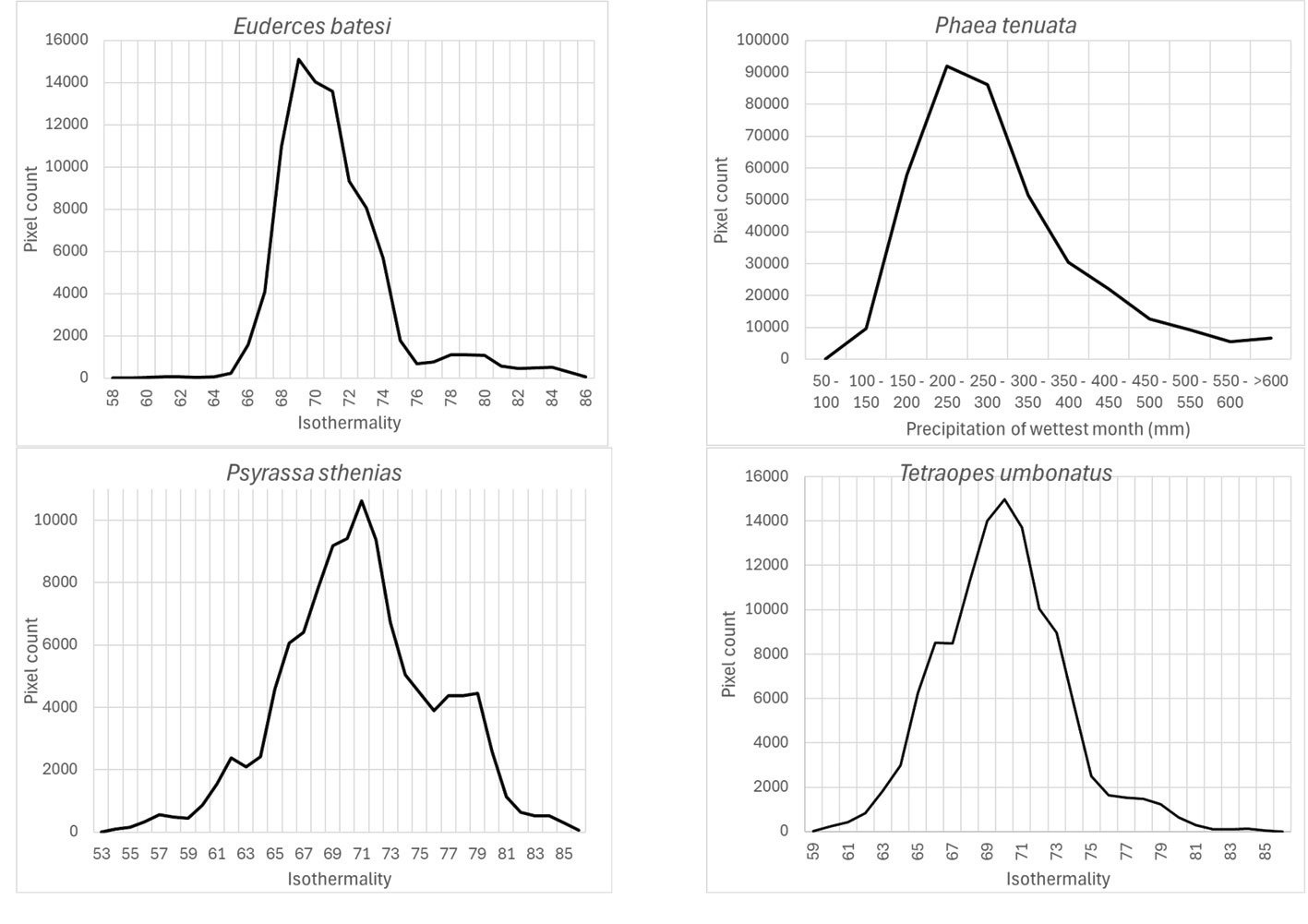
The 24 species distribution models primarily represent examples of this family’s species that are better sampled in the country. Different from relying on a single prediction algorithm, this study presents consensus models, generated from combining probability versions of 4 algorithms: Maxent, Artificial Neural Networks, Generalized Linear Model, and Support Vector Machine. The median was the statistic chosen for combining the 4 algorithms because of its characteristic of being a location parameter in contrast with the mean, which combines in-depth partial values, and is affected by outliers. Although the variations among models for the same species were evident, all 24 species distribution models showed good performance, as indicated by the AUC ratios and partial AUC values.
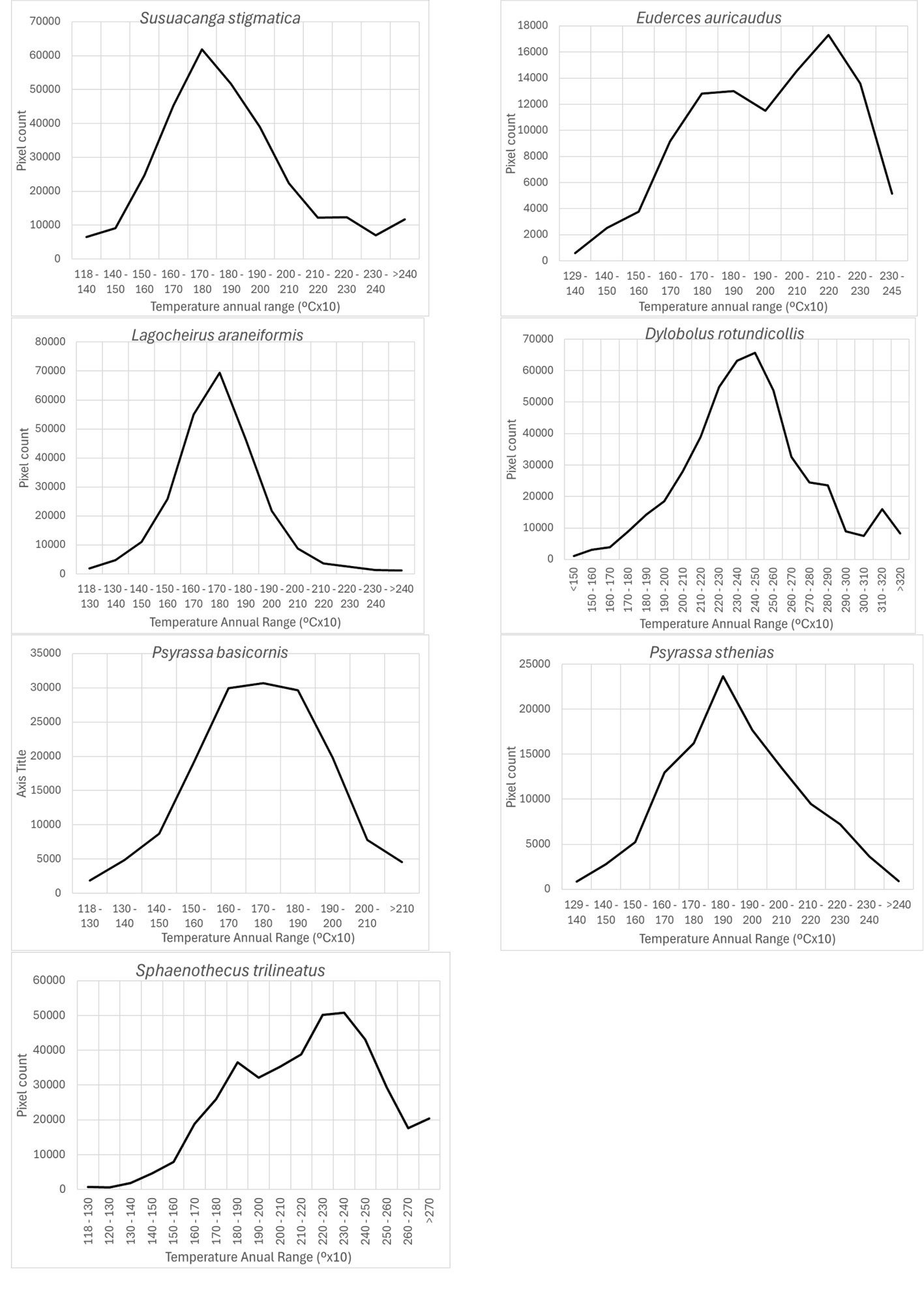
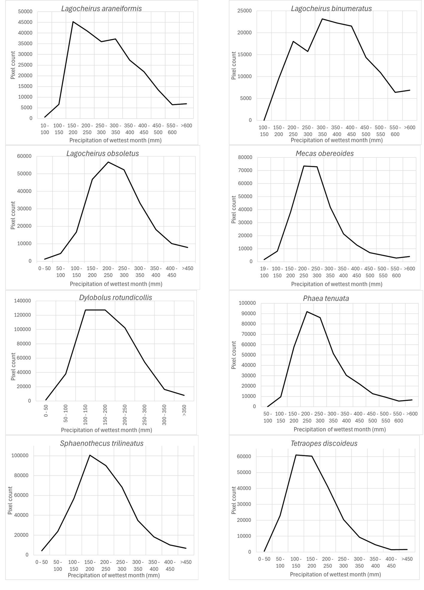
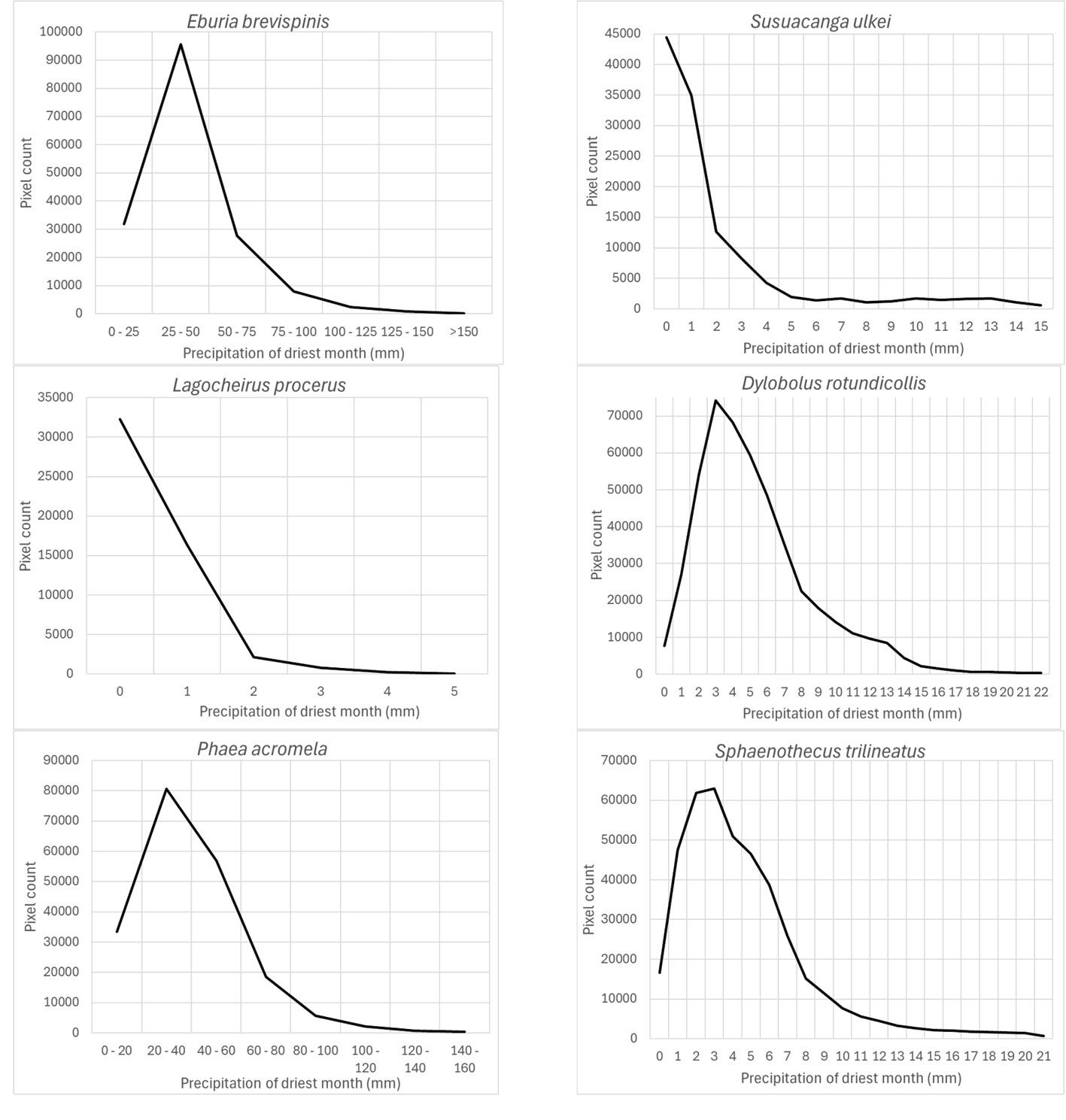
According to Maxent, prediction variables differed in importance for predicting species potential distribution models. The variables that had higher mean importance among species included precipitation seasonality (wc_bio15), precipitation of driest month (wc_bio14), temperature annual range (wc_bio7), precipitation of wettest month (wc_bio13), elevation, and isothermality (wc_bio3). As in this case, other studies on Cerambycidae, where the potential distribution of some species in this group was modeled, also showed that the predictive bioclimatic variables were diverse and contributed to the models to varying degrees. For example, for Psacothea hilaris, the predictive variables were precipitation of the warmest quarter (wc_bio18) and isothermality (wc_bio3) (Ruzzier et al., 2024); for Rosalia alpina, they were elevation and mean temperature of the driest quarter (wc_bio9) (Bosso et al., 2018); for Morimus asper, they were the maximum temperature during the warmest month (wc_bio5) and altitude (Kostova et al., 2023); for Batocera lineolata, they were maximum temperature in January, precipitation in July, and temperature seasonality (wc_bio4) (Li et al., 2020); for Xylotrechus arvicola, they were precipitation in October, mean maximum temperature in January, mean minimum temperature in July, mean maximum temperature, and mean minimum temperature in August (Felicísimo et al., 2021); for Monochamus carolinensis, they were precipitation of the warmest quarter (wc_bio18), precipitation seasonality (wc_bio15), precipitation of the coldest quarter (wc_bio19), mean diurnal range (wc_bio2), and minimum temperature of the coldest month (wc_bio5) (Zhao et al., 2023). This recorded variety in predictive environmental variables corresponds to the region where each of these studies was conducted. For P. hilaris, the main areas were Italy and the Mediterranean region; for R. alpina, it was Europe; for M. asper, it was Bulgaria; for B. lineolata, it was China; for X. arvicola, it was Spain; and for M. carolinensis, it was on a global scale.
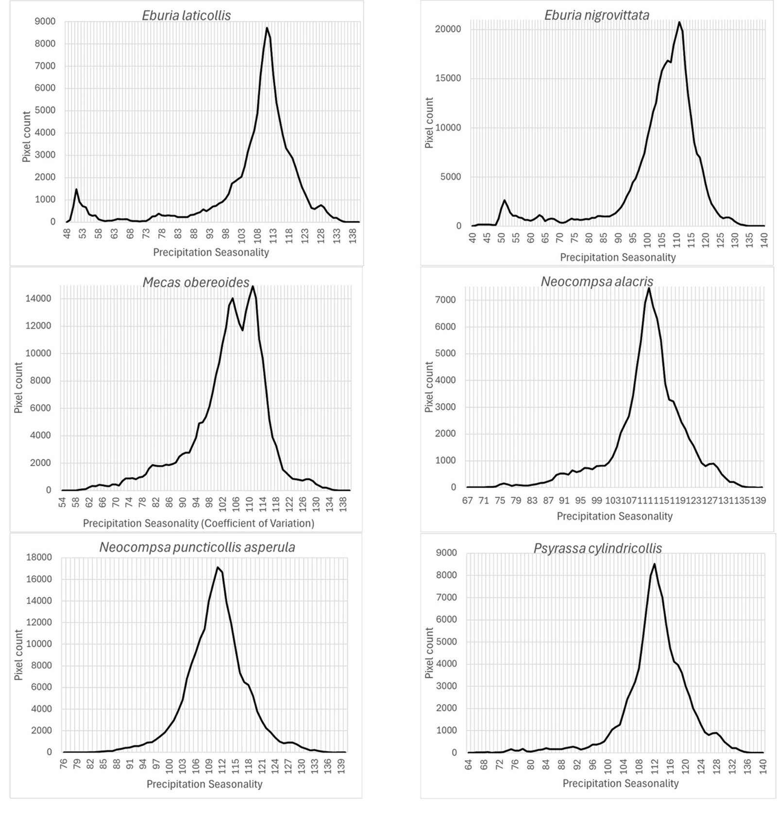
The response variables obtained by cross-tabulating the species presence models with the environmental (prediction) variables identify the most favorable habitat conditions, according to the predicted distribution models. Even though the most frequent values of the environmental variables indicate which areas dominated the species distribution, the range of such values provides an estimate of the span of environmental values where species can occur.
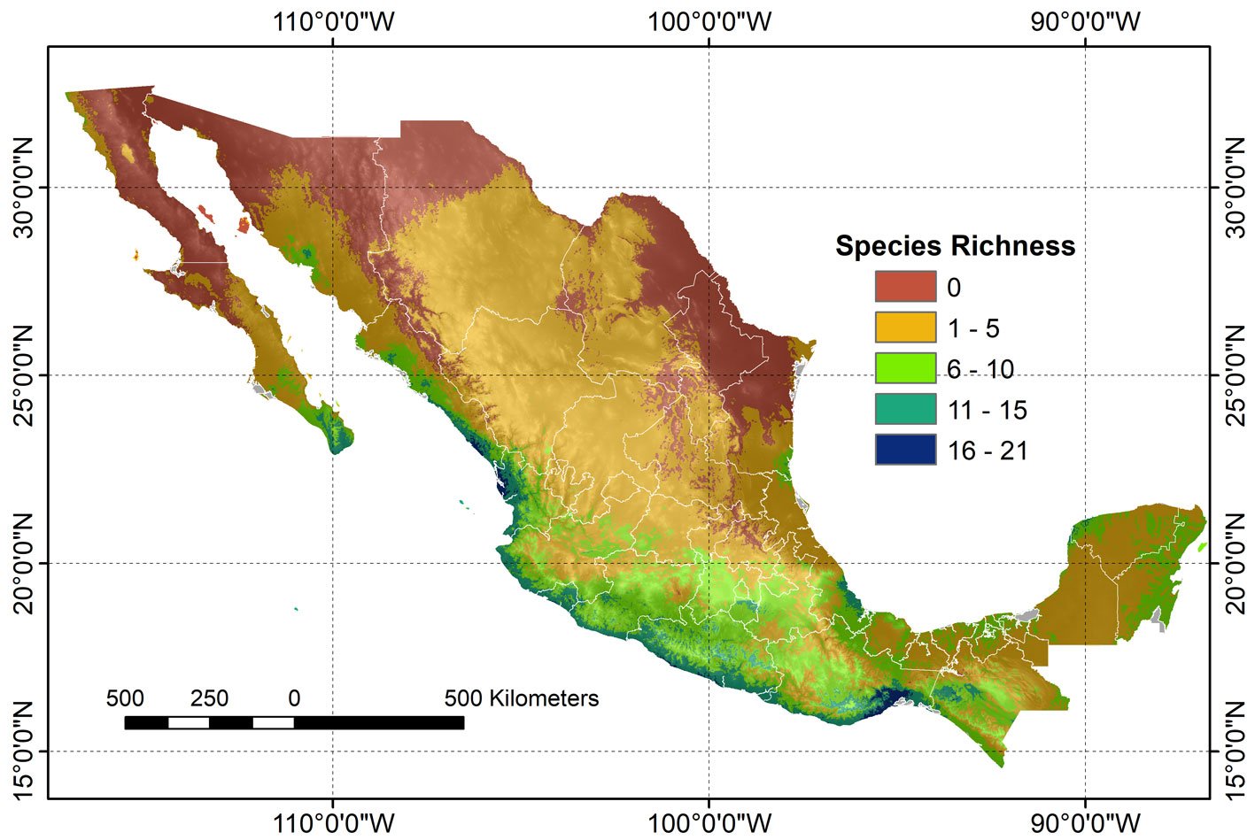
The 24 modeled species showed spatial correspondence, where the highest interval (16-21 species) is confined to restricted areas with tropical and humid tropical forests in the country. Larger species spatial correspondence areas corresponded to the lowest intervals (1-5 and 6-10 species), which were distributed in the tropical dry forest and temperate forests. It is worth mentioning that biomes such as the North American deserts and the Great Plains showed the highest proportion of areas with the absence of species.
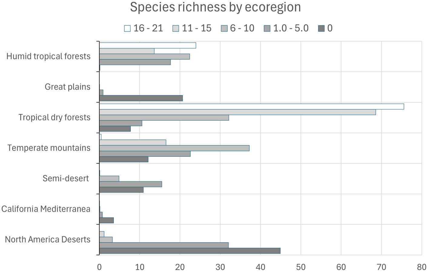
References
Anderson, R. P., & Martı́nez-Meyer, E. (2004). Modeling species’ geographic distributions for preliminary conservation assessments: an implementation with the spiny pocket mice (Heteromys) of Ecuador. Biological Conservation, 116, 167–179. https://doi-org.pbidi.unam.mx:2443/10.1016/S0006-3207(03)00187-3
Araújo, M. B., & New, M. (2007). Ensemble forecasting of species distributions. Trends in Ecology & Evolution, 22, 42–47. https://doi.org/10.1016/j.tree.2006.09.010
Austin, M. P. (2002). Spatial prediction of species distribution: an interface between ecological theory and statistical modelling. Ecological Modelling, 157, 101–118. https://doi.org/10.1016/S0304-3800(02)00205-3
Ballesteros-Mejia, L., Kitching, I. J., Jetz, W., Nagel, P., & Beck, J. (2013). Mapping the biodiversity of tropical insects: species richness and inventory completeness of African sphingid moths. Global Ecology and Biogeography, 22, 586–595. https://doi.org/10.1111/geb.12039
Ballesteros-Mejia, L., Kitching, I. J., Jetz, W., & Beck, J. (2017). Putting insects on the map: near-global variation in sphingid moth richness along spatial and environmental gradients. Ecography, 40, 698–708. https://doi.org/10.1111/ecog.02438
Barredo, J. I., Strona, G., De Rigo, D., Caudullo, G., Stancanelli, G., & San-Miguel-Ayanz, J. (2015). Assessing the potential distribution of insect pests: case studies on large pine weevil (Hylobius abietis L) and horse-chestnut leaf miner (Cameraria ohridella) under present and future climate conditions in European forests. EPPO Bulletin, 45, 273–281. https://doi.org/10.1111/epp.12208
Bezark, L. G., & Monné, M. A. (2013). Checklist of the Oxypeltidae, Vesperidae, Disteniidae and Cerambycidae, (Coleoptera) of the Western Hemisphere. Retrieved from: http://bezbycids.com/byciddb/checklists/WestHemiCerambycidae2024.pdf
Bosso, L., Smeraldo, S., Rapuzzi, P., Sama, G., & Garonna, A. P. (2018). Nature protection areas of Europe are insufficient to preserve the threatened beetle Rosalia alpina (Coleoptera: Cerambycidae): evidence from species distribution models and conservation gap analysis. Ecological Entomology, 43, 192–203. https://doi.org/10.1111/een.12485
Buse, J., Schröder, B., & Assmann, T. (2007). Modelling habitat and spatial distribution of an endangered longhorn beetle-A case study for saproxylic insect conservation. Biological Conservation, 137, 372–381. https://doi.org/10.1016/j.biocon.2007.02.025
Catalano, G. A., D’Urso, P. R., Maci, F., & Arcidiacono, C. (2023). Influence of parameters in SDM application on citrus presence in mediterranean area. Sustainability, 15, 7656. https://doi.org/10.3390/su15097656
Crawford, P. H. C., & Hoagland, B. W. (2010). Using species distribution models to guide conservation at the state level: the endangered American burying beetle (Nicrophorus americanus) in Oklahoma. Journal of Insect Conservation, 14, 511–521. https://doi.org/10.1007/s10841-010-9280-8
Colwell, R. K. (1996). Biota: the biodiversity database manager. Sinauer Associates, Sunderland, Massachusetts. Systematic Biology, 46, 574–575.
D’Amen, M., Pradervand, J. N., & Guisan, A. (2015). Predicting richness and composition in mountain insect communities at high resolution: a new test of the SESAM framework. Global Ecology and Biogeography, 24, 1443–1453. https://doi.org/10.1111/geb.12357
Drake, J. M., Randin, C., & Guisan, A. (2006). Modelling ecological niches with support vector machines. Journal of Applied Ecology, 43, 424–432. https://doi.org/10.1111/
j.1365-2664.2006.01141.x
Elith, J., Graham, C. H., Anderson, R. P., Dudík, M., Ferrier, S., Guisan, A. et al. (2006). Novel methods improve prediction of species’ distributions from occurrence data. Ecography,
29, 129–151. https://doi.org/10.1111/j.2006.0906-7590.04596.x
Eickermann, M., Junk, J., & Rapisarda, C. (2023). Climate change and insects. Insects, 14, 678. https://doi.org/10.3390/insects14080678
Elith, J., & Graham, C. H. (2009). Do they? How do they? Why do they differ? On finding reasons for differing performances of species distribution models. Ecography, 32, 66–77. https://doi.org/10.1111/j.1600-0587.2008.05505.x
Felicísimo, A. M., Armendáriz, I., & Alberdi, V. (2021). Modelling the potential effects of climate change in the distribution of Xylotrechus arvicola in Spain. Horticultural Science (Prague), 48, 38–46. https://doi.org/10.17221/85/2019-HORTSCI
Fick, S. E., & Hijmans, R. J. (2017). WorldClim 2: new 1-km spatial resolution climate surfaces for global land areas. International Journal of Climatology, 37, 4302–4315. https://doi.org/10.1002/joc.5086
Franklin, J. (2010). Mapping species distributions. Spatial inference and prediction. Cambridge UK: Cambridge University Press. https://doi.org/10.1017/CBO9780511810602
Graham, C. H., Ferrier, S., Huettman, F., Moritz, C., & Peterson, A. T. (2004). New developments in museum-based informatics and applications in biodiversity analysis. Trends in Ecology & Evolution, 19, 497–503. https://doi.org/10.1016/j.tree.2004.07.006
Guisan, A., & Zimmermann, N. E. (2000). Predictive habitat distribution models in ecology. Ecological Modelling, 135, 147–186. https://doi.org/10.1016/S0304-3800(00)00354-9
Guisan, A., Edwards, T. C., & Hastie, T. (2002). Generalized linear and generalized additive models in studies of species distributions: setting the scene. Ecological Modelling, 157, 89–100. https://doi.org/10.1016/S0304-3800(02)00204-1
Guo, Q., Kelly, M., & Graham, C. H. (2005). Support vector machines for predicting distribution of Sudden Oak Death in California. Ecological Modelling, 182, 75–90. https://doi.org/10.1016/j.ecolmodel.2004.07.012
Guo, Q., & Liu, Y. (2010). ModEco: an integrated software package for ecological niche modeling. Ecography, 33, 637–642. https://doi.org/10.1111/j.1600-0587.2010.06416.x
Hassall, C. (2012). Predicting the distributions of under-recorded Odonata using species distribution models. Insect Conservation and Diversity, 5, 192–201. https://doi.org/10.1111/j.1752-4598.2011.00150.x
Hastie, T., Tibshirani, R., & Friedman, J. (2001). The elements of statistical learning: data mining, inference, and prediction.
New York: Springer. https://doi.org/10.1007/978-0-387-21606-5
Hijmans, R. J., Cameron, S. E., Parra, J. L., Jones, P. G., & Jarvis, A. (2005). Very high resolution interpolated climate surfaces for global land areas. International Journal of Climatology: A Journal of the Royal Meteorological Society, 25, 1965–1978. https://doi.org/10.1002/joc.1276
Huntley, B., Green, R. E., Collingham, Y. C., Hill, J. K., Willis, S. G., Bartlein, P. J. et al. (2004). The performance of models relating species geographical distributions to climate is independent of trophic level. Ecology Letters, 7, 417–426. https://doi.org/10.1111/j.1461-0248.2004.00598.x
Jung, J. M., Lee, W. H., & Jung, S. (2016). Insect distribution in response to climate change based on a model: Review of function and use of CLIMEX. Entomological Research, 46, 223–235. https://doi.org/10.1111/1748-5967.12171
Kostova, R., Bekchiev, R., Popgeorgiev, G., & Kornilev, Y. V. (2023). First exhaustive distribution and habitat modelling of Morimus asper (Sulzer, 1776) sensu lato (Coleoptera, Cerambycidae) in Bulgaria. Nature Conservation, 53, 39–59. https://doi.org/10.3897/natureconservation.53.104243
Lek, S., Delacoste, M., Baran, P., Dimopoulos, I., Lauga, J., & Aulagnier, S. (1996). Application of neural networks to modelling nonlinear relationships in ecology. Ecological Modelling,90, 39–52. https://doi.org/10.1016/0304-3800(95)00142-5
Li, A., Wang, J., Wang, R., Yang, H., Yang, W., Yang, C. et al. (2020). MaxEnt modeling to predict current and future distributions of Batocera lineolata (Coleoptera: Cerambycidae) under climate change in China. Écoscience, 27, 23–31. https://doi.org/10.1080/11956860.2019.1673604
Linsley, E. G. (1961). The Cerambycidae of North America. Part I. Introduction. University of California Publications in Entomology, 18, 1–135.
Lobo, J. M. (2016). The use of occurrence data to predict the effects of climate change on insects. Current Opinion in Insect Science, 17, 62–68. https://doi.org/10.1016/j.cois.
2016.07.003
Lobo, J. M., Lumaret, J. P., & Jay-Robert, P. (2002). Modelling the species richness distribution of French dung beetles (Coleoptera, Scarabaeidae) and delimiting the predictive capacity of different groups of explanatory variables. Global Ecology and Biogeography, 11, 265–277. https://doi.org/10.1046/j.1466-822X.2002.00291.x
Ma, G., & Ma, C. S. (2022). Potential distribution of invasive crop pests under climate change: incorporating mitigation responses of insects into prediction models. Current
Opinion in Insect Science, 49, 15–21. https://doi.org/10.1016/j.cois.2021.10.006
Martínez-Hernández, J. G., Rös, M., Pérez-Flores, O., & Toledo-Hernández, V. H. (2024). Checklist of the Cerambycidae (Coleoptera: Chrysomeloidea) of Oaxaca, Mexico. Zootaxa, 5405, 185–208. https://doi.org/10.11646/zootaxa.5405.2.2
Monné, M. A. (2005). Catalogue of the Cerambycidae (Coleoptera) of the Neotropical region. Part I. Subfamily Cerambycinae. Zootaxa, 946, 17–65. https://doi.org/10.11646/zootaxa.946.1.1
Müller, K. R., Mika, S., Tsuda, K., & Schölkopf, K. (2002). An introduction to Kernel-based learning algorithms. In Yu Hen Hu, & Jenq-Neng Hwang (Eds.), Handbook of neural network signal processing. Boca-Raton: CRC Press. https://doi.org/10.1201/9781315220413
Nearns, E. H., Lord, N. P., Lingafelter, S. W., Santos, A., Miller, K. B., & Zaspel, J. M. (2017). LONGICORN ID. Retrieved from: https://cerambycids.com
Noguera, F. A. (2014). Biodiversidad de Cerambycidae (Coleoptera) en México. Revista Mexicana de Biodiversidad, 85 (Supl.), S290–S297. https://doi.org/10.7550/rmb.32966
Norberg, A., Abrego, N., Blanchet F. G., Adler, F. R., Anderson, B. J., Anttila, J. et al. (2019). A comprehensive evaluation of predictive performance of 33 species distribution models at species and community levels. Ecological Monographs, 89, e01370. https://doi.org/10.1002/ecm.1370
Peterson, A. T., Papeş, M., & Soberón, J. (2008). Rethinking receiver operating characteristic analysis applications in ecological niche modeling. Ecological Modelling, 213, 63–72. https://doi.org/10.1016/j.ecolmodel.2007.11.008
Phillips, S. J., Anderson, R. P., & Schapire, R. E. (2006). Maximum entropy modeling of species geographic distributions. Ecological Modelling, 190, 231–259. https://doi.org/10.1016/j.ecolmodel.2005.03.026
Phillips, S. J., Anderson, R. P., Dudík, M., Schapire, R. E., & Blair, M. E. (2017). Opening the black box: an open-source release of Maxent. Ecography, 40, 887–893. https://doi.org/10.1111/ecog.03049
Phillips, S. J., & Dudík, M. (2008). Modeling of species distributions with Maxent: new extensions and a comprehensive evaluation. Ecography, 31, 161–175. https://doi.org/10.1111/j.0906-7590.2008.5203.x
Pouteau, R., Meyer, J. Y., Taputuarai, R., & Stoll, B. (2012). Support vector machines to map rare and endangered
native plants in Pacific islands forests. Ecological Informatics, 9, 37–46. https://doi.org/10.1016/j.ecoinf.2012.03.003
Ruzzier, E., Lupi, D., Tirozzi, P., Dondina, O., Orioli V., Jucker, C. et al. (2024). A two‑step species distribution modeling to disentangle the effect of habitat and bioclimatic covariates on Psacothea hilaris, a potentially invasive species. Bio Invasions, 26, 1861–1881. https://doi.org/10.1007/s10530-024-03283-9
Schölkopf, B., Platt, J. C., Shawe-Taylor, J., Smola, A. J., & Williamson, R. C. (2001). Estimating the support of a high-dimensional distribution. Neural Computation, 13, 1443–1471. https://doi.org/10.1162/089976601750264965
Senay, S. D., & Worner, S. P. (2019). Multi-scenario species distribution modeling. Insects, 10, 65. https://doi.org/10.3390/insects10030065
Silva, D. P., Aguiar, A. G., & Simião-Ferreira, J. (2016). Assessing the distribution and conservation status of a long-horned beetle with species distribution models. Journal of Insect Conservation, 20, 611–620. https://doi.org/10.1007/s10841-016-9892-8
Toledo, V. H., & Corona, A. M. (2006). Patrones de distribución de la familia Cerambycidae (coleóptera). In J. J. Morrone, & J. Llorente Bosques (Eds.), Componentes bióticos principales de la entomofauna mexicana, México (pp. 425–474). México D.F.: Las Prensas de Ciencias, UNAM.
Ulrichs, C., & Hopper, K. R. (2008). Predicting insect distributions from climate and habitat data. BioControl, 53, 881–894. https://doi.org/10.1007/s10526-007-9143-8
Urbani, F., D’alessandro, P., & Biondi, M. (2017). Using Maximum Entropy Modeling (MaxEnt) to predict future trends in the distribution of high altitude endemic insects in response to climate change. Bulletin of Insectology, 70, 189–200.
Valavi, R., Guillera-Arroita, G., Lahoz-Monfort, J. J., & Elith, J. (2022). Predictive performance of presence-only species distribution models: a benchmark study with reproducible code. Ecological Monographs, 92, e01486. https://doi.org/10.1002/ecm.1486
Watts, M. J., & Worner, S. P. (2008). Comparing ensemble and cascaded neural networks that combine biotic and abiotic variables to predict insect species distribution. Ecological Informatics, 3, 354–366. https://doi.org/10.1016/j.ecoinf.2008.08.003
Williams, J. N., Seo, C., Thorne, J., Nelson, J. K., Erwin, S., O’Brien, J. M. et al. (2009). Using species distribution models to predict new occurrences for rare plants. Diversity and Distributions, 15, 565–576. https://doi.org/10.1111/j.1472-4642.2009.00567.x
Zaniewski, A. E., Lehmann, A., & Overton, J. M. (2002). Predicting species spatial distributions using presence-only data: a case study of native New Zealand ferns. Ecological Modelling, 157, 261–280. https://doi.org/10.1016/S0304-3800(02)00199-0
Zhao, J., Zou, X., Yuan, F., Luo, Y., & Shi, J. (2023). Predicting the current and future distribution of Monochamus carolinensis (Coleoptera: Cerambycidae) based on the maximum entropy model. Pest Management Science, 79, 5393–5404. https://doi.org/10.1002/ps.7753

Macroalgae assemblages in different reef zones of a tropical urban beach in Brazil
Ensambles de macroalgas en diferentes zonas arrecifales de una playa urbana tropical en Brasil
Caio Ceza da Silva-Nunes a, c, d, e, *, Edilene Maria dos Santos Pestana b, c, Cibele Conceição dos Santos b, c, Lorena Pedreira Conceição a, c, José Marcos de Castro Nunes a, c
a Universidade Estadual de Feira de Santana, Departamento de Ciências Biológicas, Programa de Pós-Graduação em Botânica, Av. Transnordestina s/n, Novo Horizonte, CEP 44036-900, Feira de Santana, Bahia, Brazil
b Universidade Federal da Bahia, Instituto de Biologia, Programa de Pós-Graduação em Biodiversidade e Evolução, Rua Barão de Jeremoabo, 668 – Campus de Ondina, CEP: 40170-115, Salvador, Bahia, Brazil
c Universidade Federal da Bahia, Instituto de Biologia, Laboratório de Algas marinhas, Rua Barão de Jeremoabo, 668 – Campus de Ondina, CEP: 40170-115, Salvador, Bahia, Brazil
d Universidade Estadual do Sudoeste da Bahia, Departamento de Ciências Exatas e Naturais, Programa de Pós-Graduação em Ciências Ambientais, Campus Universitário “Juvino Oliveira”, BR 415, Km 04 CEP: 45.700-000 Itapetinga, Bahia, Brazil
e Colégio Estadual de Tempo Integral Antônio Batista, Rua Presidente Vargas, 83 CEP: 46380-076 Candiba, Bahia, Brazil
*Corresponding author: caiobio08@gmail.com (C.C. da Silva-Nunes)
Received: 26 February 2025; accepted: 01 August 2025
Abstract
Marine macroalgae are commonly used as bioindicators because they are sensitive to environmental changes. This study aims to verify the composition of macroalgae in the intertidal region in 3 reef zones on Itapuã beach, located in Salvador-Bahia, Brazil and which presents high tourist activity. The samples were obtained in July 2017, in the intertidal zone, in 3 reef regions: Protected Region (PR), Tide Pool Region (TP) and Frontal Region (FR). In each zone, 3 transects (20 m each) were placed, in which 5 squares measuring 20 x 20 cm were arranged at random points. Additionally, individuals were collected around each transect for qualitative analysis. Dry biomass was measured, and statistical tests were carried out to obtain diversity, equitability and similarity data. Fifty-two taxa were identified, 27 Rhodophyta, 16 Chlorophyta and 9 Phaeophyceae. TP had the highest species richness (34) and diversity; however, no significant differences were found in macroalgal biomass between the 3 reef zones analyzed. This study contributes to the understanding of the composition and structure of phytobenthic communities in intertidal regions of the Bahian coast.
Keywords: Bahia; Bioindicator; Brazil; Phytobenthos
Resumen
Las macroalgas marinas se utilizan comúnmente como bioindicadores porque son sensibles a los cambios ambientales. Este estudio tiene como objetivo verificar la composición de macroalgas en la zona intermareal en 3 regiones arrecifales de la playa de Itapuã, ubicada en Salvador-Bahía, Brasil y que tiene alta actividad turística. Las muestras fueron obtenidas en julio de 2017, en la zona intermareal, en 3 regiones arrecifales: región posterior (PR), pozas de marea (TP) y región frontal (FR). En cada región, se colocaron 3 transectos (de 20 m cada uno), donde se distribuyeron aleatoriamente 5 cuadrantes de 20 x 20cm. Además, se recolectaron individuos alrededor de cada transecto para análisis cualitativo. Se midió la biomasa seca y se realizaron pruebas estadísticas para obtener datos de diversidad, equitabilidad y similitud. Se identificaron 52 taxones: 27 Rhodophyta, 16 Chlorophyta y 9 Phaeophyceae. La TP presentó la mayor riqueza de especies (34) y diversidad; sin embargo, no se encontraron diferencias significativas en la biomasa de macroalgas entre las 3 regiones arrecifales. Este estudio contribuye a la comprensión de la composición y estructura de las comunidades fitobentónicas en zonas intermareales del litoral bahiano.
Palabras clave: Bahia; Bioindicador; Brasil; Fitobentos
Introduction
The State of Bahia has the longest coastline in Brazil, 1,103 km showing a great diversity of environments: sandy beaches, coral reefs, sandstone formations, rocky shores and mangroves (Nunes & Paula, 2004a). Furthermore, it is a region that presents a great diversity of substrates and geographical features, which is reflected in the diversity of marine flora (Nunes, 2005b). Nunes and Paula (2002) divided reef formations into 3 zones: Frontal Region (FR), Protected Region (PR) and Tide Pool Region (TP). The FR is a very hydrodynamic region, where direct collision of waves occurs. The PR is the region before the lagoon and after the reef top, it may have pools and is a region protected from direct wave collision. The TP is deep and may suffer greater wave action, forming pools on the reef top, or may suffer less or no wave action, forming pools on the reef plateau.
In recent decades, coastal areas have been undergoing an intense process of urban development, which has caused significant environmental pressures and impacts, especially in benthic communities in reef formations (Costa et al., 2012; Nascimento, 2013). In Salvador, these impacts come from urban expansion, real estate speculation, tourism, human activities, such as fishing and trampling, causing the degradation of the flora and a reduction in the richness and diversity of species, especially in the composition and structure of algal communities.
Marine macroalgal communities have a great ecological role, being, together with microalgae, at the base of the food chain as primary producers, being a source of food for a large part of the marine fauna. The presence of macroalgae along the coast is responsible for softening the impact of waves on the sea coast, and also plays the role of habitat for other organisms, such as animals or as a substrate for algae (Nunes, 2010; Pedrine, 2013).
When these organisms are exposed to some human interference, they are sensitive to changes in their habitat, such as the increase in the concentration of organic matter in the water, which leads to an increase in the biomass of some algal groups, or even the depletion of some nutrient that causes the disappearance of a certain species, working as bioindicators of environmental quality. In addition, the degradation of this community’s structure favors the emergence and persistence of more resistant and opportunistic species, as well as the exclusion of more fragile species (Nascimento, 2013; Nunes, 2010).
Functional groups of algae are based on similarities in their morphological and anatomical characteristics, in addition to their ecological characteristics. Steneck and Dethier (1994) grouped algae into 7 categories, these being microalgae, filamentous, foliaceous, cylindrical-corticate, coriaceous, articulated calcareous and encrusting. In the model proposed by Steneck and Dethier (1994), it is highlighted that environments of high productivity and low disturbance present high biomass and diversity of morphofunctional groups, providing an abundance of coriaceous and cylindrical-cortical algae, as they have a relatively large size and a longer life cycle.
Knowledge about macroalgae on the coast of Bahia has been expanded through taxonomic studies, with the metropolitan area of Salvador being one of the main regions of the State’s coast studied, for example: Altamirano and Nunes (1997), Amorin et al. (2006), Barreto et al. (2004), Macedo et al. (2009), Marins et al. (2008), Nunes (1998a, b, 1999, 2005a, b), Nunes and Guimarães (2008, 2009, 2010), Nunes and Paula (2000, 2001, 2002, 2004a, b, 2006), Nunes et al. (2005).
Studies regarding the community structure of marine macroalgae have been carried out on the Brazilian coast. The majority are concentrated in the subtidal zone, namely, Amado Filho et al. (2003), Figueiredo et al. (2004), Villaça et al. (2010) in Rio de Janeiro, Oliveira-Carvalho et al. (2003) in Pernambuco, and Horta et al. (2008) in Santa Catarina. And in the intertidal zone, Barbosa et al. (2008) in Espírito Santo, and Muñoz and Pereira (1997) in Pernambuco. In Bahia, there are studies by Caires et al. (2013), Costa et al. (2012), and Ferreira et al. (2022), who carried out studies in the intertidal zone, and Costa Jr. et al. (2002) and Marins et al. (2008) in the subtidal zone. Although the coast of Bahia is the longest in Brazil, studies aimed to understand the structure of phytobenthic communities are scarce, creating a gap in the knowledge of these communities.
The present study analyzes the intertidal phytobenthic community in 3 reef zones of Itapuã beach, aiming to identify and compare differences in the composition and structure of the species between the studied areas, using the Feldmann and Cheney indices as bioindicators of local environmental characteristics.
Materials and methods
Itapuã beach is located in Salvador, Bahia in Brazil (Fig. 1), and corresponds to 2 large rocky bodies, and has coarse sand beaches, many reefs and rocky bollards (Nunes, 1998b). The collection was carried out on July 11, 2017, in the intertidal region, during low spring tide. The intertidal region was compartmentalized into the 3 regions proposed by Nunes and Paula (2002). Nunes (2010) was followed for the collection protocol.
Three 20 m transects were placed in each zone and arranged parallel to the coastline. In each transect, 5 squares measuring 20 x 20 cm were previously drawn. All material contained in the square was removed using a spatula. For qualitative analysis, specimens were collected around each transect. The collected material was placed in plastic bags or polyethylene bottles, fixed with 4% formalin. All material from the collections was taken to the Marine Algae Laboratory (LAMAR), at the Biology Institute of the Federal University of Bahia, where it was analyzed using a stereomicroscope (Leica© – Zoom 2000) to separate and identify the epiphytic algae.
Taxon identification was done using an Olympus© – CX 22 microscope. Blades were assembled from freehand cuts, made with the aid of razor blades and box cutters. Calcareous algae were analyzed based on prior decalcification by immersing the samples in 0.6 M nitric acid. For specific identification, references commonly used in phycology were used (Dawes & Mathieson, 2008; Littler & Littler, 2000; Nunes, 2005b; Nunes & Guimarães, 2008; Nunes & Paula, 2000, 2001, 2002). For the arrangement of taxa, the taxonomic arrangement of Guiry and Guiry (2025) was mainly followed.
For the analysis of dry biomass, the infrageneric taxa were previously identified, separated and dried in an oven at 60 ºC for 48 hours and weighed until constant biomass was obtained. The results are presented in grams/m² of dry weight. The results for each reef zone were compared regarding the total number of taxa, and dry biomass using Shannon-Wiener diversity (H’) and Pielou equitability (J) indexes.
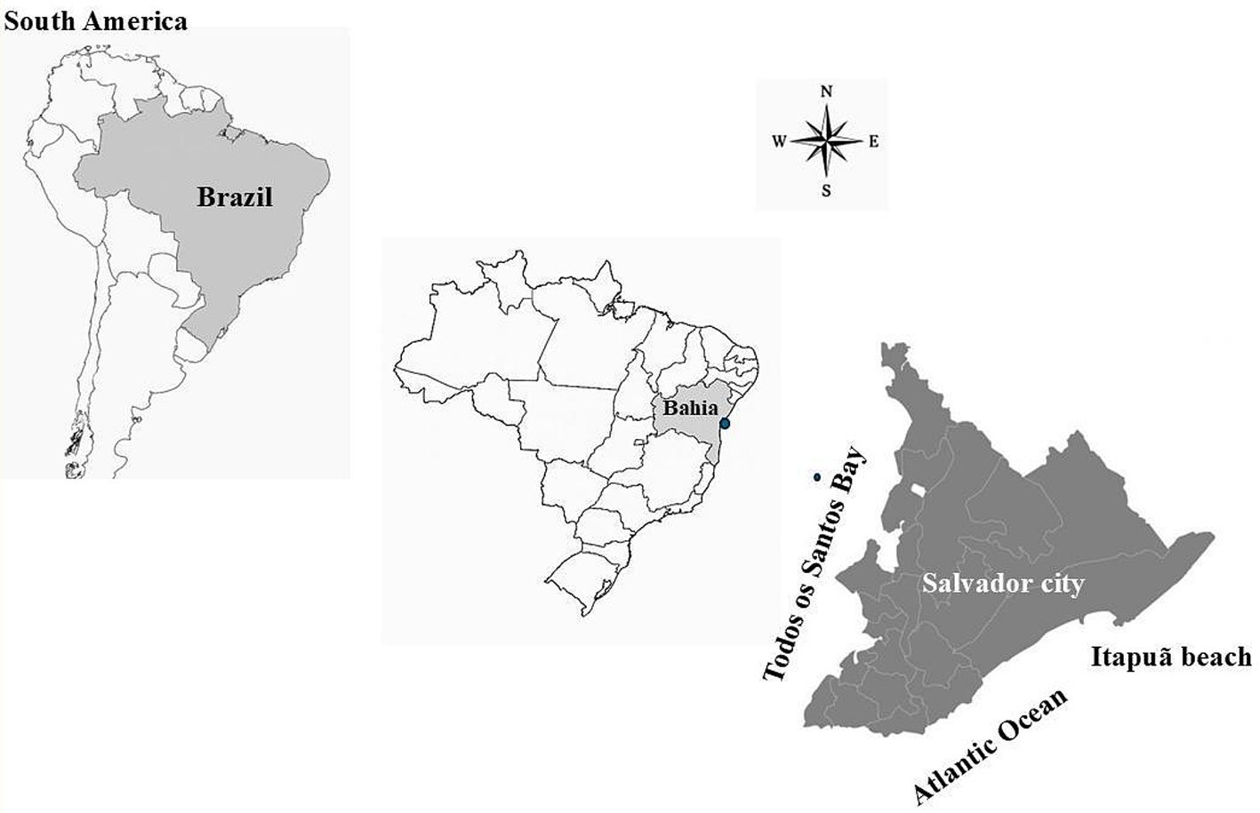
Using the macroalgae biomass data found in each reef zone, the Kruskal-Wallis test was performed to check whether there was a significant difference between the biomass recorded in the different zones. The Bray-Curtis similarity index was also calculated with the biomass data and Non-metric Multidimensional Scaling (nMDS) was performed using the transformed data. ANOSIM was performed for values in which there was a significant difference between the similarity results. The analyses were carried out using SigmaPlot 12 and Primer V6 software.
The species dominance index is used to assess how much one or a few species stand out in relation to the others within a biological community. It considers the proportion of individuals or the biomass of each species, allowing us to identify which of them exert the greatest influence on the structure and functioning of the ecosystem. The higher the value of the index, the greater the dominance, which indicates that a few species concentrate the majority of the individuals present. On the other hand, lower values reflect a more balanced and diverse community, with a lower concentration of individuals in a few species (Melo, 2008).
Simpson’s dominance index was used, calculated as D = ∑ (ni/N) 2, where ni is the number of individuals of a species and N is the total number of individuals of all species in the community. The value of D varies between 0 and 1, with values close to 1 indicating high dominance, that is, few species dominate the environment, while values close to 0 indicate greater diversity and balanced distribution among species.
The Feldmann index (obtained by dividing the number of species of Rhodophyta by that of Phaeophyceae [R/P]) and the Cheney index (adding the number of species of Rhodophyta to that of Chlorophyta, and dividing this value by the number of browns [R + C/ P]) (Figueiredo et al., 2008).
Results
Fifty-two taxa were identified, 27 (52) belonging to the Rhodophyta, 16 (31) Chlorophyta, and 9 (17) Phaeophyceae (Heterokontophyta). Table 1 presents the taxa, their distribution throughout the 3 zones of the reef and their respective morphotypes.
Among the zones, TP presented the greatest species richness (34) with Rhodophyta as the most representative group, 17 taxa, followed by Chlorophyta (11) and Phaeophyceae (6). Chaetomorpha minima, Gayliella dawsonii, Gracilaria ferox, Lejolisia mediterranea, Ptilothamnion speluncarum, and Stylonema alsidii were unique to this environment. PR was second in terms of species richness, such as Caulerpa chemnitzia, Caulerpa sertularioides, Cladophora corallinicola, Hypnea pseudomusciformis, Hypnea sp. 1, and Melanothamnus gorgoniae only occurred in this region. FR presented the lowest richness among the environments, such as Ceramium corniculatum, Codium taylori, Dictyopteris jamaicensis, Dictyopteris polypodioides, Sphacelaria tribuloides, and Wrangelia argus, all exclusive for the region. However, it is worth highlighting a greater representation of rhodophytes for the protected and FR.
Among the species found, 16 occurred in all regions such as Amansia multifida, Amphiroa anastomosans, Anadyomene stellata, Bryopsis pennata, Colpomenia sinuosa, Crouania attenuata, Dictyopteris delicatula, Dictyosphaeria versluysii, Dictyota mertensii, Gelidiella acerosa, Halimeda opuntia, Jania pedunculata var. adhaerens, Palisada perforata, Phyllodictyon anastomosans, Ulva flexuosa, and Ulva rigida.
Regarding the morphotypes, among the 52 taxa found, 19 were filamentous, 17 cylindrical-corticates, 9 foliaceous, 3 articulated calcareous, 3 encrusting and 1 coriaceous. Cylindrical-corticate algae were well represented in the 3 regions, predominating in the PR, followed by foliaceous algae; in the TP, the filamentous morphotype was the one with the highest representation, followed by cylindrical-corticated and foliaceous ones, the same pattern was observed in the FR.
The diversity of analysis based on the Shannon-Wiener index, showed that the TP is more diverse than the others, followed by the PR, and finally by the FR. Dominance values are inversely proportional to diversity values, which shows that in the FR, there is dominance of one or a few species over the others (Table 2).
In table 3, biomass data and the percentage of contribution of each macroalgae in the zone biomass are presented. The average total biomass of each zone was 108.01 g.m-2 in the FR, 48.83 g.m-2 in tide pool and 474.59 g.m-2 in the PR. The Kruskal-Wallis test showed that no significant differences were found in macroalgal biomass between the three reef zones analyzed (Kruskal-Wallis p = 0.869). However, the ordering of the sampling points according to the presence/absence of macroalgae (Fig. 2) shows the dispersion of samples in the 3 zones, mainly samples from the PR. The ANOSIM analysis (Table 4) shows that there was a significant difference between the FR and the TP, and between the FR and the PR, but there was no significant difference between the PR and the TP. The Feldmann and Cheney indices (Fig. 3) for the 3 reef regions studied were consistent with the flora of tropical and warm temperate regions.
Table 1
List of taxa found in the reef zones on Itapuã beach and their respective morphotypes: PR = Protected Region; TP = Tide Pool; FR = Frontal Region. Morphotypes: FT = filamentous; FC = foliaceous; CC = cylindrical corticates; CR = coriaceous; AC = articulated calcareous; E = encrusting. Presence (+) and absence (–).
| Taxa | PR | TP | FR | Morphotype |
| Chlorophyta | ||||
| Ulvophyceae | ||||
| Bryopsidales | ||||
| Bryopsidaceae | ||||
| Bryopsis pennata J.V. Lamouroux | + | + | + | FT |
| Caulerpaceae | ||||
| Caulerpa chemnitzia (Esper) J.V. Lamouroux | + | – | – | CC |
| C. racemosa (Forsskål) J. Agardh | + | + | + | CC |
| C. sertularioides (S.G. Gmelin) M. Howe | + | – | – | CC |
| Codiaceae | ||||
| Codium taylorii P.C. Silva | – | – | + | CC |
| Halimedaceae | ||||
| Halimeda opuntia (Linnaeus) J.V. Lamouroux | + | + | + | AC |
| Ulva flexuosa Wulfen | + | + | + | FC |
| U. rigida C. Agardh | + | + | + | FC |
| Cladophorales | ||||
| Anadyomenaceae | ||||
| Anadyomene stellata (Wulfen) C. Agardh | + | + | + | FC |
| Boodleaceae | ||||
| Phyllodictyon anastomosans (Harvey) Kraft & M.J. Wynne | + | + | + | FT |
| Cladophoraceae | ||||
| Chaetomorpha minima Collins & Hervey | – | + | – | FT |
| Cladophora corallinicola Sonder | + | – | – | FT |
| C. laetevirens (Dillwyn) Kützing | – | + | + | FT |
| C. vagabunda (Linnaeus) Hoek | + | – | + | FT |
| Siphonocladaceae | ||||
| Dictyosphaeria versluysii Weber Bosse | + | + | + | E |
| Valoniaceae | ||||
| Valonia aegagropila C.Agardh | + | + | – | CC |
| Heterokontophyta | ||||
| Phaeophyceae | ||||
| Dictyotales | ||||
| Dictyotaceae | ||||
| Dictyopteris delicatula J.V. Lamouroux | + | + | + | FC |
| D. jamaicensis W.R. Taylor | – | – | + | FC |
| D. polypodioides (De Candolle) J.V. Lamouroux | – | – | + | FC |
| Dictyota mertensii (C.Martius) Kützing | + | + | + | FC |
| Table 1. Continued | ||||
| Taxa | PR | TP | FR | Morphotype |
| Padina antillarum (Kützing) Piccone | + | + | – | FC |
| Spatoglossum schroederi (C. Agardh) Kützing | – | + | + | FC |
| Ectocarpales | ||||
| Scytosiphonaceae | ||||
| Colpomenia sinuosa (Mertens ex Roth) Derbès & Solier | + | + | + | E |
| Fucales | ||||
| Sargassaceae | ||||
| Sargassum polyceratium Montagne | – | + | + | CR |
| Sphacelariales | ||||
| Sphacelariaceae | ||||
| Sphacelaria tribuloides Meneghini | – | – | + | FT |
| Rhodophyta | ||||
| Florideophyceae | ||||
| Ceramiales | ||||
| Callithamniaceae | ||||
| Crouania attenuata (C. Agardh) J. Agardh | + | + | + | FT |
| Ceramiaceae | ||||
| Ceramium corniculatum Montagne | – | – | + | FT |
| Centroceras clavulatum (C. Agardh) Montagne | + | – | – | FT |
| Gayliella dawsonii (A.B. Joly) Barros-Barreto & F.P. Gomes | – | + | – | FT |
| Ceramothamnion brasiliensis (A.B. Joly) M.J. Wynne & C.W. Schneider | + | – | + | FT |
| Rhodomelaceae | ||||
| Alsidium triquetrum (S.G. Gmelin) Trevisan | – | + | – | CC |
| Amansia multifida J.V. Lamouroux | + | + | + | CC |
| Digenea simplex (Wulfen) C. Agardh | + | + | – | CC |
| Herposiphonia bipinnata M. Howe | – | + | – | FT |
| H. tenella (C. Agardh) Ambronn | – | + | – | FT |
| Melanothamnus gorgoniae (Harvey) Díaz-Tapia & Maggs | + | – | – | FT |
| Palisada perforata (Bory) K.W. Nam | + | + | + | CC |
| Wrangeliaceae | ||||
| Lejolisia mediterranea Bornet | – | + | – | FT |
| Ptilothamnion speluncarum (Collins & Hervey) D.L. Ballantine & M.J. Wynne | – | + | – | FT |
| Wrangelia argus (Montagne) Montagne | – | – | + | FT |
| Corallinales | ||||
| Corallinaceae incrustante | ||||
| Jania pedunculata var. adhaerens (J.V. Lamouroux) A.S. Harvey, Woelkerling & Reviers | + | + | + | AC |
| Corallinaceae incrustante | + | – | + | E |
| Lithophyllaceae | ||||
| Table 1. Continued | ||||
| Taxa | PR | TP | FR | Morphotype |
| Amphiroa anastomosans Weber-van Bosse | + | + | + | AC |
| Gelidiales | ||||
| Gelidiaceae | ||||
| Gelidium capense (S.G. Gmelin) P.C. Silva | + | – | + | CC |
| Gelidiellaceae | ||||
| Gelidiella acerosa (Forsskål) Feldmann & Hamel | + | + | + | CC |
| G. ligulata E.Y. Dawson | + | – | + | CC |
| Gigartinales | ||||
| Cystocloniaceae | ||||
| Hypnea pseudomusciformis Nauer, Cassano & M.C. Oliveira | + | – | – | CC |
| Hypnea sp.1 | + | – | – | CC |
| Gigartinaceae | ||||
| Chondracanthus acicularis (Roth) Fredericq | + | + | – | CC |
| Gracilariales | ||||
| Gracilariaceae | ||||
| Gracilaria ferox J. Agardh | – | + | – | CC |
| Nemaliales | ||||
| Galaxauraceae | ||||
| Galaxaura rugosa (J. Ellis & Solander) J.V. Lamouroux | – | + | + | CC |
| Stylonematophyceae | ||||
| Stylonematales | ||||
| Stylonemataceae | ||||
| Stylonema alsidii (Zanardini) K.M. Drew | – | + | – | FT |
| Total | 33 | 34 | 32 |
Discussion
Rhodophyta was the most representative group in the present study, followed by Chlorophyta and Phaeophyceae. This pattern has been observed in other studies on phytobenthic macroalgal communities as typical on the Brazilian coast (Braga et al., 2014; Costa et al., 2012; Ferreira et al., 2022). It should be noted that rhodophytes tend to dominate the environment in the absence of large brown algae in tropical environments, suggesting that there is competition between algae that use different strata in the phytobenthic community (Figueiredo et al., 2004). Furthermore, studies have confirmed the decline of Phaeophyceae at the same rate that Chlorophyta species have been increasing, which can be attributed to the negative effects of anthropogenic impact on the coastal environment (Oliveira & Qi, 2003; Scherner et al., 2013). Representatives of Phaeophyceae are more sensitive to pollutants (heavy metals and excess organic matter produced by sewage), which can even negatively affect the germination and cell division of these organisms (Kevekordes, 2001). Representatives of Chlorophyta, such as species of Ulva Linnaeus, have the capacity of benefit from contamination by pollutants, being considered opportunistic species (Scherner et al., 2012).
Table 2
Shannon-Wiener Diversity index, dominance and equitability of macroalgae in the intertidal region of Itapuã beach.
| Region | Shannon-Wiener | Dominance | Equability (J’) |
| Frontal Region | 3.466 | 0.0312 | 1 |
| Tide Pool | 3.526 | 0.0294 | 1 |
| Protected Region | 3.497 | 0.0303 | 1 |
The taxa that contributed most to the average biomass of macroalgae found on Itapuã beach were Amphiroa anastomosans, Digenea simplex, Gelidiella acerosa, and Sargassum polyceratium. It has been previously reported that algae with greater structural complexity, such as corticate algae, are better adapted to environments with greater hydrodynamics and luminosity, as this morphotype confers greater resistance to desiccation (Costa et al., 2012; Villaça et al., 2008).
Table 3
Biomass and percentage of contribution of macroalgae species in the constitution of biomass in each of the zones studied: FR = Frontal Region, TP = Tide Pool, and PR = Protected Region. Pi = Percentage of importance.
| Taxa | FR (g.m-2) | Pi | TP (g.m-2) | Pi (%) | PR (g.m-2) | Pi (%) |
| Amphyroa anastomosans | 70.07 | 64.87 | 15.76 | 32.28 | 31.59 | 6.66 |
| Anadyomene stellata | 1.41 | 1.31 | 1.76 | 3.61 | 0.00 | 0.00 |
| Bryopsis pennata | 0.00 | 0.00 | 0.20 | 0.42 | 0.00 | 0.00 |
| Caulerpa racemosa | 1.42 | 1.32 | 0.00 | 0.00 | 0.00 | 0.00 |
| C. sertularioides | 0.00 | 0.00 | 0.00 | 0.00 | 1.11 | 0.23 |
| Centroceras clavulatum | 0.00 | 0.00 | 0.00 | 0.00 | 0.25 | 0.05 |
| Chondracanthus acicularis | 0.00 | 0.00 | 0.00 | 0.00 | 0.00 | 0.00 |
| Cladophora vagabunda | 0.00 | 0.00 | 0.00 | 0.00 | 0.15 | 0.03 |
| Colpomenia sinuosa | 0.16 | 0.15 | 0.08 | 0.15 | 0.00 | 0.00 |
| Dictyopteris delicatula | 5.42 | 5.01 | 5.48 | 11.22 | 0.00 | 0.00 |
| D. jamaicensis | 0.00 | 0.00 | 0.00 | 0.00 | 0.00 | 0.00 |
| Dictyosphaeria versluysii | 0.67 | 0.62 | 0.25 | 0.51 | 0.09 | 0.02 |
| Dictyota mertensii | 0.00 | 0.00 | 0.00 | 0.00 | 1.13 | 0.24 |
| Digenea simplex | 0.00 | 0.00 | 0.97 | 1.98 | 430.92 | 90.80 |
| Gelidiellaceae | 0.00 | 0.00 | 2.00 | 4.09 | 0.00 | 0.00 |
| Gelidium sp. 1 | 0.00 | 0.00 | 0.94 | 1.92 | 0.19 | 0.04 |
| Gelidium sp. 2 | 0.00 | 0.00 | 0.00 | 0.00 | 0.09 | 0.02 |
| Gelidiella acerosa | 14.27 | 13.21 | 5.97 | 12.24 | 2.69 | 0.57 |
| G. ligulata | 0.71 | 0.66 | 0.00 | 0.00 | 0.00 | 0.00 |
| Halimeda opuntia | 0.31 | 0.29 | 2.14 | 4.38 | 0.48 | 0.10 |
| Hypnea sp. 1 | 0.40 | 0.37 | 0.00 | 0.00 | 0.00 | 0.00 |
| Hypnea sp. 2 | 0.00 | 0.00 | 0.00 | 0.00 | 0.00 | 0.00 |
| Jania pedunculata var. adhaerens | 7.60 | 7.03 | 0.00 | 0.00 | 0.27 | 0.06 |
| Lobophora variegata | 0.00 | 0.00 | 0.39 | 0.80 | 0.00 | 0.00 |
| Padina antillarum | 0.00 | 0.00 | 2.26 | 4.64 | 1.15 | 0.24 |
| Palisada perforata | 4.86 | 4.50 | 0.00 | 0.00 | 0.05 | 0.01 |
| Phyllodictyon anastomosans | 0.00 | 0.00 | 0.00 | 0.00 | 0.00 | 0.00 |
| Sargassum polyceratium | 0.00 | 0.00 | 9.69 | 19.85 | 0.00 | 0.00 |
| Spatoglossum schroederi | 0.10 | 0.09 | 0.00 | 0.00 | 0.00 | 0.00 |
| Ulva rigida | 0.63 | 0.58 | 0.83 | 1.69 | 3.55 | 0.75 |
| Valonia aegagropila | 0.00 | 0.00 | 0.11 | 0.22 | 0.86 | 0.18 |
| Total | 108.01 | 48.83 | 474.59 |
The difference found in macroalgae biomass between reef zones can be explained by the hydrodynamics to which they are exposed on the reef, being wave action the main responsible for the spatial distribution of the community on the reef. The movement of waves helps to obtain nutrients, favoring the productivity of macroalgae and thus increasing biomass, however this only applies to those algae that have adaptations to resist the impact of waves, as they are also responsible for removing macroalgae from the substrate (Diez et al., 2003; Hurd et al., 1996; Leigh et al., 1987).
The highest biomasses were found in FR and PR. The FR is constantly submerged and this favors the establishment of algae, as they are submerged for longer, suffer less desiccation and are less exposed to direct sunlight. The lowest biomass values were recorded in the TP, a region that retains water during low tide, however the algae are subjected to intense solar radiation, high salinity and water temperature. The negative effects of these stressors result in lower biomass and also there is less hard substrate for fixation (Costa et al., 2012; Villaça et al., 2010).
Table 4
Results of ANOSIM tests for significance of differences between sample groups based on observed macroalgal species distribution data.
| Reef regions | (Global R= 0.613; significance level = 0.4%) | |
| Region pairs | Statistical R | Level |
| FR, TP | 0.815 | 10 |
| FR, PR | 0.667 | 10 |
| TP, PR | 0.481 | 20 |


The dominance of filamentous, cylindrical-corticate and foliaceous morphotypes was observed, corroborating the model by Orfanidis et al. (2001), which proposes that impacted environments should have a greater abundance of algae with intensely branched (corticated), laminar (foliaceous) and filamentous thallus, characterized by high growth rates and a short life cycle (annual). However, conserved environments would have an abundance of algae with thick thallus (coriaceous), articulated calcareous and encrusting, cacterized by low growth rates and a long life cycle (perennial), which reflected in the low representation of articulated, encrusting and coriaceous calcareous morphotypes. In a study carried out by Nascimento (2013) in Salvador and the North Coast of Bahia, the foliaceous and cylindrical-corticate morphotypes were more representative in both impacted and preserved environments, highlighting the predominance of these morphotypes.
The distribution of algae according to morphofunctional groups reflects the conditions of reef zones, since each taxa has its adaptive characteristics. Cylindrical-cortical algae were well represented in the 3 reef zones, with a predominance in the PR, as this morphology confers greater resistance to desiccation, helping these algae to establish themselves in different environments (Costa et al., 2012; Villaça et al., 2008). Tide pool region was dominated by filamentous algae, morphotype usually associated with benthic communities in early successional stages as they show rapid growth (Braga et al., 2014).
Regarding phytogeography, the Feldmann (F) and Cheney (C) indices found for the different regions of the Itapuã reef characterized the PR and the TP as tropical and the FR as warm temperate, according to the classification proposed by Horta et al. (2001). Factors such as the greater hydrodynamism in the FR may justify this classification in relation to its algal community, since the increase in the number of species of brown algae is noticeable as one approaches the FR. Bouzon et al. (2006), studying floristic and phytogeographic aspects of marine macroalgae in the Bays of Santa Catarina, attributed the variations in the Feldmann and Cheney indices to the exclusion of species of brown algae and the favoring of opportunistic species of red and green algae; in this study, lower values of these indices were recorded in the frontal zones and in the pool zone, where the richness of species of brown algae was greater.
Understanding the composition and structure of phytobenthic communities on the Brazilian coast, as well as on the coast of Bahia is extremely important. Despite the vast coastal extension, there are few studies referring to the algal community structure in intertidal zone as most studies focus on the subtidal zone. Also, most studies on the composition and structure of phytobenthic communities are restricted to the state of Rio de Janeiro. More studies should be carried out along the coast of Bahia to fill the gaps and alternating dry and rainy periods and/or comparing the reef zones of different beaches in the intertidal zone. The results suggest that the Itapuã reefs are in a good state of conservation.
Acknowledgements
CCSN, acknowledges the post-doctoral scholarship to the State University of Southwest Bahia (UESB) – Notice 266/2023.; CCSN, LPC, EMSP, to the Coordination for the Improvement of Higher Education Personnel – Brazil (CAPES), finance code 001; CCS, to the Bahia Research Support Foundation (FAPESB – T.O. B., No. BOL0416/2017) for a scholarship.; JMCN, to the National Council for Scientific and Technological Development (CNPq), Brazil for the research productivity fellowship (308261/2022-4).
References
Altamirano, M., & Nunes, J. M. C. (1997). Contribuciones al macrofitobentos del Município de Camaçari (Bahia, Brasil). Acta Botanica Malacitana, 22, 211–215. https://doi.org/10.24310/abm.v22i0.8639
Amado Filho, G. M., Barreto, M. B. B., Marins, B. V., Felix, C., & Reis, R. P. (2003). Estrutura das comunidades fitobentônicas do infralitoral da Baía de Sepetiba, RJ, Brasil. Revista Brasileira de Botânica, 26, 329–342. https://doi.org/10.1590/s0100-84042003000300006
Amorin, P. R. R., Moura, C. W. N., & Moniz-Brito, K. L. (2008). Estudo morfotaxonômico das espécies de Halimeda, Penicillus e Udotea (Bryopsidales, Chlorophyta) do Recife de Franja da Ilha de Itaparica, Bahia. Anais do XI Congresso Brasileiro de Ficologia & Simpósio Latino-Americano sobre Algas Nocivas. Rio de Janeiro: Museu Nacional. Série Livros.
Barbosa, S. O., Figueiredo, M. A. O., & Testa, V. (2008). Structure and dynamic of benthic communities dominated by macrophytes in praia de Jacaraípe, Espírito Santo, Brazil. Hoehnea, 35, 563–575. https://doi.org/10.1590/S2236-89062008000400008
Barreto, M. B. B., Brasileiro, P. S., Nunes, J. M. C., & Amado-Filho, G. M. (2008). Algas marinhas bentônicas do sublitoral das formações recifais da Baía de Todos os Santos, BA – 1. Novas ocorrências. Hoehnea, 31, 321–330.
Braga, A. C. S., Tâmega, F. T. S., Pedrini, A. G., & Muniz, R. A. (2014). Composição e estrutura da comunidade fitobentônica do infralitoral da praia de Itaipu, Niterói, Brasil: Subsídios para monitoramento e conservação. Iheringia. Série Botânica, 69, 267–276. https://isb.emnuvens.com.br/iheringia/article/view/90
Bouzon, J. L., Salles, J. P., Bouzon, Z., & Horta, P. A. (2006). Aspectos florísticos e fitogeográficos das macroalgas marinhas das baías da ilha de Santa Catarina, SC,Brasil. Insular, 35, 69–84.
Caires, T. A., Costa, I. O., Jesus, P. B. D., Matos, M. R. B. D., Pereira-Filho, G. H., & Nunes, J. M. D. C. (2013). Evaluation of the stocks of Hypnea musciformis (Rhodophyta: Gigartinales) on two beaches in Bahia, Brazil. Brazilian Journal of Oceanography, 61, 65–71. https://doi.org/10.1590/S1679-87592013000100007
Costa-Júnior, O. S., Attrill, M. J., Pedrini, A. G., & De Paula, J. C. (2002). Spatial and seasonal distribution of seaweeds on coral reefs from Southern Bahia, Brazil. Botanica Marina, 45, 346–355. https://doi.org/10.1515/BOT.2002.035
Costa, I. O., Caires, T. A., Pereira-Filho, G. H., & Nunes, J. M. C. (2012). Macroalgas bentônicas associadas a bancos de Hypnea musciformis (Wulfen) J.V. Lamour. (Rhodophyta-Gigartinales) em duas praias do litoral baiano. Acta Botanica Brasilica, 26, 493–507. https://doi.org/10.1590/S0102-33062012000200025
Dawes, C., & Mathieson, A. (2008). The seaweeds of Florida. Gainesville: University of Florida Press.
Diez, I., Santolaria, A., & Gorostiaga, J. M. (2003). The relationship of environmental factors to the structure and distribution of subtidal seaweed vegetation of the western Basque coast (N Spain). Estuarine, Coastal and Shelf Science, 56, 1041–1054. https://doi.org/10.1016/S0272-7714(02)00301-3
Ferreira, S. M. C., Lolis, L. A., Noga, P. M., Affe, H. M. J., & Nunes, J. M. C. (2022). A highly diverse phytobenthic community along a short coastal reef gradient in northeastern Brazil. Universitas Scientiarum, 27, 34–56. https://doi.org/10.11144/Javeriana.SC271.ahdp
Figueiredo, M. A. O., Barreto, M. B. B., & Reis, R. P. (2004). Caracterização das macroalgas nas comunidades marinhas da área de Proteção Ambiental de Cairuçú, Parati, RJ – Subsídios para futuros monitoramentos. Revista Brasileira de Botânica, 27, 11–17. https://doi.org/10.1590/S0100-84042004000100002
Figueiredo, M. A. O., Horta, P.A., Pedrini, A. G., & Nunes, J. M. C. (2008). Benthic marine algae of the coral reefs of Brazil: a literature review. Oecologia Brasiliensis, 12, 259–270. https://doi.org/10.4257/oeco.2008.1202.07
Guiry, M. D., & Guiry, G. M. (2025). AlgaeBase. World-wide electronic publication, University of Galway. Retrieved on February 21, 2025 from: https://www.algaebase.org
Horta, P. A., Amancio, E., Coimbra, C. S., & Oliveira, E. C. (2001). Considerações sobre a distribuição e origem da flora de macroalgas marinhas brasileiras. Hoehnea, 28, 243–265.
Horta, P. A., Salles, J. P., Bouzon, J., Scherner, F., Cabral, D., Bouzon, Z. L. et al. (2008). Composição e estrutura dos fitobentos do infralitoral da Reserva Biológica Marinha do Arvoredo, Santa Catarina, Brasil —implicações para a conservação. Oecologia Brasiliensis, 12, 51–57. https://doi.org/10.4257/oeco.2008.1202.06
Hurd, C. L., Harrison, P. J., & Druehl, L. D. (1996). Effect of seawater velocity on inorganic nitrogen uptake by morphologically distinct forms of Macrocystis integrifolia from wave-sheltered and exposed sites. Marine Biology, 126, 205–214. https://doi.org/10.1007/BF00347445
Kevekordes, K. (2001). Toxicity tests using developmental stages of Hormosira banksii (Phaeophyta) identify ammonium as a damaging component of secondary treated sewage effluent discharged into Bass Strait, Victoria, Australia. Marine Ecology Progress Series, 219, 139–148. https://doi.org/10.3354/meps219139
Leigh, E. G., Paine, R. T., Quinn, J. F., & Suchanek, T. H. (1987). Wave energy and intertidal productivity. Proceedings of the National Academy of Sciences, 84, 1314–1318. https://doi.org/10.1073/pnas.84.5.1314
Littler, D. S., & Littler, M. M. (2000). Caribbean reef plants. An identification guide to the reef plants of the Caribbean, Bahamas, Florida and Gulf of Mexico. Washington D.C.: OffShore Graphics.
Macedo, T. S., Varjão, A. S., Fernandes, L. L., Silva, D. F., Almeida, J. S., Messias, J. C. et al. (2009). Levantamento taxonômico e diversidade das macroalgas marinhas bentônicas da praia da Pituba, Salvador, Bahia. Revista Eletrônica de Biologia, 2, 29–39.
Marins, B. V., Brasileiro, P. A., Barreto, M. B. B., Nunes, J. M. C., Yoneshigue-Valentin, Y., & Amado-Filho, G. M. (2008). Subtidal benthic marine algae of the Todos os Santos Bay, Bahia State, Brazil. Oecologia Brasiliensis, 12, 229–242. https://doi.org/10.4257/oeco.2008.1202.05
Melo, A. S. (2008). O que ganhamos “confundindo” riqueza de espécies e equabilidade em um índice de diversidade? Biota Neotropica, 8, 21–27. https://doi.org/10.1590/s1676-06032008000300001
Muñoz, A. O. M., & Pereira, S. M. B. (1997). Caracterização quali-quantitativa das comunidades de macroalgas nas formações recifais da praia do Cupe Pernambuco, Brasil. Trabalhos Oceanográficos da Universidade Federal do Pernambuco, 25, 93–109. https://doi.org/10.5914/tropocean.v25i1.2731
Nascimento, O. S. (2013). Impactos da urbanização sobre a estrutura, cobertura de morfotipos funcionais e heterogeneidade química das comunidades de algas
recifais (M.Sc. Thesis). Instituto de Biologia, Universidade Federal da Bahia, Salvador.
Nunes, J. M. C. (1998a). Catálogo de algas marinhas bentônicas do Estado da Bahia. Acta Botanica Malacitana, 23, 5–21. https://doi.org/10.24310/abm.v23i0.8547
Nunes, J. M. C. (1998b). Rodofíceas marinhas bentônicas da orla oceânica de Salvador, Estado da Bahia, Brasil. Insula, 49, 27–37.
Nunes, J. M. C. (1999). Phaeophyta da Região Metropolitana de Salvador, Bahia, Brasil (M.Sc. Thesis). Instituto de Biociências, Universidade de São Paulo, São Paulo.
Nunes, J. M. C. (2005a). A família Liagoraceae (Rhodophyta, Nemaliales) no Estado da Bahia, Brasil. Hoehnea, 32, 429–444.
Nunes, J. M. C. (2005b). Rodofíceas marinhas bentônicas do Estado da Bahia, Brasil (Ph.D. Thesis). Instituto de Biociências, Universidade de São Paulo, São Paulo.
Nunes, J. M. C. (2010). Taxonomia morfológica: metodologia de trabalho. In A. G. Pedrini (Org.), Macroalgas: uma introdução à Taxonomia (pp. 53–70). Rio de Janeiro, Rio de Janeiro: Technical Books.
Nunes, J. M. C., & Guimarães, S. M. P. B. (2008). Novas referências de rodofíceas marinhas bentônicas para o litoral brasileiro. Biota Neotrópica, 8, 89–100. https://doi.org/10.1590/S1676-06032008000400008
Nunes, J. M. C., & Guimarães, S. M. P. B. (2009). Primeira referência de plantas gametofíticas em Spermothamnion nonatoi (Ceramiales, Rhodophyta). Rodriguésia, 60, 259–264. https://www.jstor.org/stable/23499987
Nunes, J. M. C., & Guimarães, S. M. P. B. (2010). Morfologia y toxonomía de Scinaia halliae (Scinaiaceae, Rhodophyta) em el litoral de Bahia y Espírito Santo, Brasil. Revista
de Biología Marina y Oceonografía, 45, 159–164. http://dx.doi.org/10.4067/S0718-19572010000100017
Nunes, J. M. C., & Paula, E. J. (2000). Estudos taxonômicos do gênero Padina Adanson (Dictyotaceae – Phaeophyta) no litoral do Estado da Bahia, Brasil. Acta Botanica Malaci-
tana, 26, 21–43. https://doi.org/10.24310/abm.v25i0.8470
Nunes, J. M. C., & Paula, E. J. (2001). O gênero Dictyota Laumouroux (Dictyotaceae – Phaeophyta) no litoral do Estado da Bahia, Brasil. Acta Botanica Malacitana, 26, 5–18. https://doi.org/10.24310/abm.v26i0.7375
Nunes, J. M. C., & Paula, E. J. (2002). Composição e distribuição das Phaeophyta nos Recifes da Região Metropolitana de Salvador, Bahia, Brasil. Iheringia, 57, 113–130.
Nunes, J. M. C., & Paula, E. J. (2004a). Chnoosporaceae, Scytosiphonaceae, Sporochnaceae e Sphacelariaceae (Phaeophyta) no Estado da Bahia, Brasil. Biotemas, 17, 7–28.
Nunes, J. M. C., & Paula, E. J. (2004b). Estudos taxonômicos de Ectocarpaceae e Ralfsiaceae (Phaeophyta) da Região Metropolitana de Salvador, Ba, Brasil. Acta Biologica Leopoldensia, 26, 37–50.
Nunes, J. M. C., & Paula, E. J. (2006). O gênero Dictyopteris J.V.Lamour. (Dictyotaceae – Phaeophyta) no estado da Bahia, Brasil. Hidrobiológica, 16, 251–258. https://hidro
biologica.izt.uam.mx/index.php/revHidro/article/view/1036
Nunes, J. M. C., Santos, A. C. C., & Santana, L. C. (2005). Novas ocorrências de algas marinhas bentônicas para o Estado da Bahia, Brasil. Iheringia Série Botânica,60,
99–106. https://isb.emnuvens.com.br/iheringia/article/view/209
Oliveira, E. C., & Qi, Y. (2003). Decadal changes in a polluted bay as seen from its seaweed flora: the case of Santos Bay in Brazil. AMBIO: A Journal of the Human Environment, 32, 403–405. https://doi.org/10.1579/0044-7447-32.6.403
Orfanidis, S., Panayotidis, P., & Stamatis, N. (2001). Ecological evaluation of transitional and coastal waters: a marine benthic macrophytes-based model. Mediterranean Marine Science, 2, 45–65. https://doi.org/10.12681/mms.266
Pedrini, A. G. (2013). Macroalgas (ocrófitas multicelulares) marinhas do Brasil. Rio de Janeiro, Rio de Janeiro: Technical Books.
Scherner, F., Barufi, J. B., & Horta, P. A. (2012). Photosynthetic response of two seaweed species along an urban pollution gradient: evidence of selection of pollution-tolerant species. Marine Pollution Bulletin, 64, 2380–2390. https://doi.org/10.1016/j.marpolbul.2012.08.012
Scherner, F., Horta, P. A., De Oliveira, E. C., Simonassi, J. C., Hall-Spencer, J. M., Chow, F. et al. (2013). Coastal urbanization leads to remarkable seaweed species loss and community shifts along the SW Atlantic. Marine Pollution Bulletin, 76, 106–115. https://doi.org/10.1016/j.marpolbul.2013.09.019
Steneck, R. S., & Dethier, M. N. (1994). A functional group approach to the structure of algal-dominated communities. Oikos, 69, 476-498. http://dx.doi.org/10.2307/3545860
Villaça, R., Yoneshigue-Valentin, Y., & Boudouresque, C. F. (2008). Estrutura da comunidade de macroalgas do infralitoral do lado exposto da ilha de Cabo Frio (Arraial do Cabo, RJ). Oecologia Brasiliensis, 12, 206–221. https://doi.org/10.4257/oeco.2008.1202.03
Villaça, R., Carvalhal-Fonseca, A., Jensen, V. K., & Knoppers, B. (2010). Species composition and distribution of macroalgae on Atol das Rocas, Brazil, SW Atlantic. Botanica Marina, 53, 113–122. https://doi.org/10.1515/BOT.2010.013
Zar, J. H. (2010). Biostatistical analysis. Upper Saddle River, New Jersey: Prentice Hall International.

Panmictic population of the pollinating moth Tegeticula baja(Lepidoptera: Prodoxidae), across the distribution of its plant hosts
Población panmíctica de la polilla polinizadora Tegeticula baja (Lepidoptera: Prodoxidae) a lo largo de la distribución de sus plantas hospederas
Maria Clara Arteaga a, *, C. Rocio Alamo-Herrera a, Anna Darlene van der Heiden a, b, Nicole Sicaeros-Samaniego a
a Centro de Investigación Científica y de Educación Superior de Ensenada, Departamento de Biología de la Conservación,
Carr. Tijuana-Ensenada 3918, Zona Playitas, 22860 Ensenada, Baja California, Mexico
b Uppsala University, Department of Medical Biochemistry and Microbiology, Hursagatan 3, 752 37, Uppsala, Sweden
*Corresponding author: arteaga@cicese.mx (M.C. Arteaga)
Received: 14 March 2025; accepted: 24 July 2025
Abstract
Ecological interactions and demographic history shape the genetic diversity of populations. Tegeticula baja is the specialist pollinator of different Yucca hosts in the Baja California Peninsula, a region that experienced changes in habitat distribution during the Pleistocene. To assess the effects of host specificity and historical changes in habitat configuration, we i) analyzed the genetic structure of moth populations associated with 3 different Yucca plant species, ii) identified signatures of historical demographic changes, and iii) reconstructed the past potential distribution of T. baja at different periods. We genotyped the COI of 128 moths from 39 locations and estimated genetic diversity, population structure, and demographic history. We found an overall haplotype diversity of 0.708 and a nucleotide diversity of 0.0015. Moth populations associated with the 3 hosts exhibited similar diversity levels, with no evidence of genetic structure. These findings suggest that ecological associations with different host plants do not drive T. baja diversification. Instead, its demographic history has played a more significant role in shaping the levels and the distribution of the genetic diversity.
Keywords: Ecological interaction; Genetic diversity; Historical demography; Insect-plant association; Population structure; Yucca
Resumen
Las interacciones ecológicas y la historia demográfica moldean la diversidad genética de las poblaciones. Tegeticula baja es una polinizadora especialista de diferentes yuccas hospederas en la península de Baja California, una región que experimentó cambios en la distribución de los hábitats durante el Pleistoceno. Para evaluar los efectos de la especificidad del huésped y los cambios históricos en la configuración de los hábitats, i) analizamos la estructura genética de las poblaciones de polillas asociadas a distintos hospederos, ii) identificamos señales de cambios demográficos históricos y iii) reconstruimos su distribución potencial en el pasado. Genotipificamos el COI de 128 polillas de 39 localidades y estimamos la diversidad genética, la estructura poblacional y la historia demográfica. Encontramos una diversidad haplotípica global de 0.708 y una diversidad nucleotídica de 0.0015. Las poblaciones de polillas asociadas a las 3 especies de plantas mostraron niveles de diversidad similares, sin evidencia de estructura genética. Estos hallazgos sugieren que la asociación ecológica con diferentes plantas huésped no impulsa la diversificación de T. baja. En cambio, su historia demográfica ha desempeñado un papel más importante en la configuración de su diversidad genética.
Palabras clave: Interacciones ecológicas; Diversidad genética; Historia demográfica; Asociación planta-insecto; Estructura poblacional; Yucca
Introduction
The ecological interaction between pollinator insects and their host plants plays a crucial role in shaping the distribution and genetic diversity of the species involved, influencing processes such as natural selection, genetic drift, and gene flow among populations (Futuyma, 2000; Gloss et al., 2013, 2016). Additionally, other factors, such as geographic distance (e.g., Driscoe et al., 2019) and demographic history shaped by past climatic changes (e.g., Liu et al., 2016; Smith et al., 2011), can influence the amount of genetic variation within populations and its spatial distribution.
Moths of the genus Tegeticula Zeller are specialist pollinators of the genus Yucca Linnaeus, maintaining an obligate mutualism (Engelmann, 1872; Pellmyr, 2003). Generally, each Tegeticula species pollinates a single Yucca species. However, few moth species pollinate multiple Yucca species (Althoff et al., 2006, 2012). During the flowering period, adult moths emerge and mate within Yucca flowers. The female uses specialized mouthparts to collect pollen and transfer it to other flowers. Upon arrival, she inserts her ovipositor into the ovary to lay her eggs. After, she deposits the pollen onto the flower’s stigma, ensuring fertilization and fruit development, from which the larvae will feed on a small portion of the seeds (Engelmann, 1872; Pellmyr, 2003). This obligate interaction between yucca and yucca moths influences the gene flow, facilitating differentiation and diversification processes in both pollinators and host plants (Arteaga et al., 2020; Leebens-Mack & Pellmyr, 2004; Leebens-Mack et al., 1998)
Yucca plants and yucca moths are distributed across North America (Pellmyr et al., 2008). This region has experienced changes in habitat distribution due to Pleistocene climatic fluctuations, which have impacted the genetic diversity and structure of both Yucca populations and their pollinators (Alemán et al., 2024; Arteaga et al., 2020; De la Rosa et al., 2020; Smith et al., 2011). In the Baja California Peninsula (BCP), Mexico, Tegeticula baja Pellmyr is an endemic moth species distributed from the central to the southern part of the peninsula. This moth pollinates 2 endemic Yucca species and their hybrid populations, which exhibit an allopatric distribution: Yucca valida Brandegee occurs in the arid ecosystems of the Central Desert and the northern Magdalena Plains, hybrid populations are found in the southern Magdalena Plains (Arteaga et al., 2020), and Y. capensis Lenz is located in the tropical dry forest of southern BCP (Lenz, 1998; Pellmyr et al., 2008; Turner et al., 1995).
The flowering phenology of these endemic Yucca species and their hybrid populations is asynchronous and influenced by water availability. Yucca valida blooms from April to July (Turner et al., 1995), hybrid populations flower in August and September, and Y. capensis blooms from September to October (Arteaga et al., 2015; Lenz, 1998). The asynchronous flowering limits the temporal coexistence of moths from different populations, as each group responds to the floral signals of its host plant. Additionally, these moths exhibit short-distance dispersal (Álamo-Herrera et al., 2022). Consequently, the temporal availability of floral resources and the limited dispersal of these pollinators may contribute to genetic structuring among populations across their distribution.
Given the obligate interaction between pollinators and plants, we hypothesize that distinct genetic lineages of T. baja are associated with each host Yucca species, influenced by geographic distances and asynchronous flowering. Additionally, considering historical habitat changes in the BCP (Dolby et al., 2015), we expect an impact on the species’ demographic history. Specifically, we i) examined the genetic structure among moth populations associated with each Yucca species and their hybrids, ii) identified signals of historical population changes, and iii) determined how the distribution of suitable conditions for the species has changed over time. This study will contribute to a better understanding of how ecological interactions and historical environmental changes shape the genetic diversity of pollinating moths in the Yucca-Tegeticula mutualism.
Materials and methods
We visited 75 localities where the endemic yuccas and their hybrids were found (Fig. 1A). We collected 3 to 5 fruits from at least 5 plants per locality. We dissected the fruits and examined them for the presence of T. baja larvae, which are typically found among the seeds. We stored the larvae in 96% ethanol and preserved them at -80 °C. We collected a total of 128 moth larvae from 39 of the 75 localities (Fig. 1A), including 16 sites of Yucca valida (N = 49), 8 of Y. capensis (N = 39), and 15 of hybrid plants (N = 40).
We used 20 mg of larval tissue for DNA extraction following the commercial kit “Qiagen DNeasy Blood & Tissue Kit” protocol. We amplified a fragment of the Cytochrome Oxidase subunit I (COI) marker using primers S1461 (5’-ACAATTTATCGCCTAAACTTCAGCC-3’) and A2302 (5’-CTACAAATCCTAATAATCCATTG-3’; Smith et al., 2009). The PCR mixture consisted of 5 μl of buffer (1X), 2 μl of MgCl (2 mM), 0.4 μl of dNTPs (0.6 mM), 0.2 μl of Taq polymerase (1U), 1 μl of each primer (0.4 mM each), 3 μl of DNA, and 12.4 μl of molecular-grade water, for a total reaction volume of 25 μl. Thermocycler conditions were: initial denaturation at 95 °C for 3 min, 35 cycles of denaturation at 94 °C for 30 s, annealing at 48 °C for 45 s, extension at 72 °C for 1 min, and a final elongation at 72 °C for 1 min. We verified the amplification quality using 1% agarose gels. PCR products were sequenced by SeqXcel (www.seqxcel.com). We also tested protocols for amplifying the nuclear EF1α gene and 9 nuclear microsatellites previously used in other species of the same genus (Drummond et al., 2010; Smith et al., 2008); however, amplifications were unsuccessful.
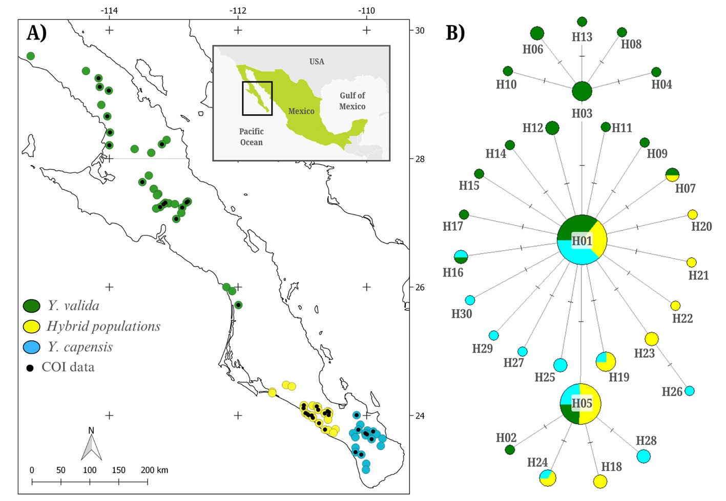
We visualized and edited COI sequences using MEGA X 4.0 and aligned them with MUSCLE (Tamura et al., 2007). We estimated the genetic diversity for the complete dataset and separately for individuals collected in locations from Y. valida, Y. capensis, and the hybrid Y. valida × Y. capensis using DNAsp (Rozas et al., 2003). We calculated the number of polymorphic sites (PS), number of haplotypes (H), haplotype diversity (h), and nucleotide diversity (π). To explore genealogical relationships, we constructed a haplotype network using the Median-Joining method in NETWORK 5.0 (Bandelt et al., 1999). Finally, to assess genetic structure among moths associated with different host plants, we implemented an analysis of molecular variance (AMOVA) using Arlequin (Excoffier et al., 2005).
We assessed the demographic history of T. baja using 3 methods. First, we conducted Tajima’s D test using DNAsp (Rozas et al., 2003). Negative values indicate population expansion, while positive values suggest population reduction (Nakamura et al., 2018). Second, we performed a mismatch distribution analysis in Arlequin, where an unimodal distribution suggests population expansion, while a multimodal distribution indicates a stable population size (Rogers & Harpending, 1992). Finally, we conducted a Bayesian Skyline Plot (BSP) analysis (Drummond et al., 2005) using BEAST 2.6.0 (Bouckaert et al., 2014). As input data, we used the commonly reported nucleotide substitution rate for COI in arthropods (1.77% divergence per lineage per million years; Papadopoulou et al., 2010), a strict molecular clock, and the HKY substitution model defined in JmodelTest2 (Darriba et al., 2012). We ran 100 million steps, sampling every 10,000 generations in the MCMC method. We calculated the effective sample size (ESS) value and constructed the BSP using TRACER 1.7 (Rambaut et al., 2018).
Table 1
Genetic diversity of Tegeticula baja based on the mitochondrial COI marker. The table includes the host plant, sample size (N), number of polymorphic sites (PS), number of haplotypes (H), haplotype diversity (h), and nucleotide diversity (π).
| Host yucca plant | N | PS | H | h | π |
| Yucca valida | 49 | 14 | 17 | 0.733 | 0.0016 |
| Hybrid populations | 40 | 9 | 10 | 0.750 | 0.0015 |
| Yucca capensis | 39 | 11 | 11 | 0.617 | 0.0012 |
We built species distribution models to assess changes in the geographic distribution of suitable conditions for Tegeticula baja and to support the interpretation of its genetic diversity and demographic history estimates. We considered 4 time periods: present (years 1970-2000), mid-Holocene (6,000 years ago), Last Glacial Maximum (22,000 years ago), and Last Interglacial (120,000 – 140,000 years ago). We constructed the models using the 75 sampling points obtained in this study, the 19 bioclimatic variables from the WorldClim 2.1 database (Fick & Hijmans, 2017), and the MAXENT software (Phillips et al., 2006), with 80% of the data used for training and 20% for validation. We configured 2,000 iterations and 10 replicates. The model evaluation included the area under the curve (AUC) and binomial probabilities, where an AUC > 0.9 reflects excellent predictive capacity.

Results
The alignment of 128 sequences resulted in 767 bp with 27 polymorphic sites, defining 30 haplotypes (NCBI ID: PX127684-PX127713; Fig. 1B). The overall haplotype diversity was moderate (h = 0.708), and nucleotide diversity was low (π = 0.0015). Moth populations associated with the 3 host plants exhibited similar diversity levels (Table 1). The haplotype network indicated that haplotypes were closely related, and that the most abundant haplotype was widely distributed among the 3 moth populations pollinating different host plants (Fig. 1B). The AMOVA revealed that the variance among moths associated with different host plants was low and not significant (Fst = 0.011, p = 0.13). In contrast, most variation was found within populations.
Since no signs of genetic structure were detected, demographic analyses and niche modeling were conducted considering all individuals as a panmictic population. Demographic analyses provided evidence of a historical population expansion. Tajima’s D test showed significant negative values (D = -2.27970, p < 0.01), and the mismatch analysis distribution was unimodal (Fig. 2A). Consistently, the BSP analysis suggested a population expansion beginning approximately 25,000 years ago (Fig. 2B).
The species distribution models, with high predictive power (AUC > 0.9), revealed historical changes in the extent and distribution of environmentally suitable areas for T. baja (Fig. 3). During the Last Interglacial (120 ka), the distribution was limited to 2 areas, one in the central and other in the southern regions of the peninsula. During the Last Glacial Maximum (22 ka) and the mid-Holocene (6 ka), an expansion occurred in both regions. Finally, in the present period (1970-2000), the potential distribution of suitable conditions for these moths is observed to be continuously present along the western portion of the peninsula, connecting the central and southern regions.
Discussion
In the obligate mutualism between Yucca plants and Tegeticula moths, the distribution of feeding and oviposition resources provided by host plants determines the presence of moths in the landscape. In this study, we evaluated the genetic structure of Tegeticula baja populations associated with different Yucca species with allopatric distributions. Contrary to our expectations, we found a single panmictic population of pollinator moths throughout its geographic range. Additionally, we detected signals of historical demographic expansion. This suggests that the ecological association with different hosts is not driving the diversification of this species and that its historical demography has played a more relevant role in the distribution of its genetic diversity.
The genetic structure of a species is influenced by multiple factors, such as dispersal capacity, the intensity of ecological interactions, and the climatic history of the areas it inhabits (Driscoe et al., 2019; Futuyma, 2000; Smith et al., 2011). Specifically, T. baja has a limited dispersal distance per generation, and only 1 generation per year (~ 42 m; Álamo-Herrera et al., 2022); its host plants have a discontinuous distribution in the current landscape, and they also exhibit asynchronous flowering (Arteaga et al., 2020; Lenz, 1998; Turner et al., 1995). Together, these factors suggested that we could find genetic structure among moth populations associated with different Yucca species. However, we did not observe significant genetic differentiation. It is possible that the age of origin of its host plants and changes in the distribution of suitable habitat conditions could partially explain this pattern.

The divergence between the 2 endemic Yucca species of the BCP is estimated to have occurred approximately 500,000 years ago (Alemán et al., 2024). The formation of hybrid populations is even a more recent event, proposed to have occurred during the Pleistocene, around 21,000 years ago, when favorable climatic conditions allowed the co-occurrence of Y. valida and Y. capensis in the same region (Arteaga et al., 2020). This period of change in host plant distribution likely also influenced the distribution of the moth Tegeticula baja. Species distribution models and demographic analyses support this, indicating a population expansion beginning around 25,000 years ago, followed by a stabilization phase approximately 3,000 years ago. These historical changes in habitat configuration likely shaped the demographic history of the moth, reducing the potential for genetic divergence across its range due to alternating periods of population isolation and secondary contact. Although the current distribution of host plants is fragmented, the slow generational turnover of T. baja, with 1 generation per year, suggests that insufficient time has passed for genetic drift to produce detectable genetic structure.
The phylogeographic pattern of Tegeticula baja does not exhibit genetic structuring associated with host plant identity, which contrasts with that of other Tegeticula species, where genetic differentiation is correlated with either geographic distance or Yucca host species. For example, T. yucasella exhibits high genetic differentiation associated with geographic distance and interactions with different Yucca species (Leebens-Mack & Pellmyr, 2004). Similarly, T. maculata, the pollinator of Hesperoyucca Engelmann, exhibits genetic clades associated with the biogeographic history of its region (Althoff et al., 2007; Segraves & Pellmyr, 2001). Although all these studies, including ours, used the same mitochondrial marker (COI subunit), we did not detect genetic differentiation in our samples. These differences between our findings and previous reports may be related to the spatial scale, which is much larger in the study of T. yucasella, and to the time of origin and biogeographic history of the host plants in the case of T. maculata (Segraves & Pellmyr, 2001).
The levels of genetic diversity detected in the panmictic population of T. baja were moderate. In particular, moths associated with Y. valida exhibited a higher number of haplotypes, possibly due to their larger geographic range (Fig. 1A). The overall nucleotide diversity was low (π = 0.0015), falling below values reported for other species in the genus, such as T. antithetica and T. synthetica (π = 0.004 and 0.005, respectively; Smith et al., 2008). This pattern of low genetic diversity observed in T. baja may be related to the historical demographic growth detected in this species. A similar pattern was reported in the panmictic population of the parasitoid wasp Digonogastra sp., which interacts with 2 Tegeticula species in the BCP (π = 0.002; Álamo-Herrera et al., 2024). This supports the idea that the levels and distribution of genetic variation in these moths are more related to their historical demography than to their ecological interactions.
In conclusion, integrating genetic data with species distribution models allows us to understand how the climatic history of the BCP has influenced the distribution of genetic diversity and demographic changes in this species. Since the moths’ life cycle depends on Yucca flowering, which in turn responds to precipitation, climate change is likely to affect the population dynamics of these insects. Periods of extreme drought, such as those occurring in recent decades in the peninsula, may impact moth demography and exacerbate a population decline. Future studies focusing on the ecology and evolution of Prodoxus species associated with Yucca and Hesperoyucca in this region could enhance our understanding of the hidden diversity within this group and complement existing information on the northern species (Smith & Leebens-Mack, 2024).
Acknowledgements
The authors are grateful to Lita Castañeda and Mario Salazar for their help with laboratory analysis, technical support, and assistance in the fieldwork. They also thank Alberto López Alemán for his valuable assistance in improving the English language of the manuscript. This study was supported financially by Secretaría de Ciencia, Humanidades, Tecnología e Innovación (Secihti) (CB-2014-01-238843, infra-2014-1-226339). The Rufford Foundation also provided financial support for a part of this study (RSG 13704-1) and the Jiji Foundation. The authors thank the Associate Editor and the anonymous reviewers for their valuable comments. The authors declare no conflicts of interest.
References
Álamo-Herrera, C. R., Arteaga, M. C., Bello-Bedoy, R., & Rosas-Pacheco, F. (2022). Pollen dispersal and genetic diversity of Yucca valida (Asparagaceae), a plant involved in an obligate pollination mutualism. Biological Journal of the Linnean Society, 136, 364–374. https://doi.org/10.1093/biolinnean/blac031
Álamo-Herrera, C. R., Arteaga, M. C., & Bello-Bedoy, R. (2024). Genetic diversity and phenotypic variation in a parasitoid wasp involved in the yucca – yucca moth interaction. Revista Mexicana de Biodiversidad, 95, e955461. https://doi.org/10.22201/ib.20078706e.2024.95.5461
Alemán, A., Arteaga, M. C., Gasca-Pineda, J., & Bello-Bedoy, R. (2024). Divergent lineages in a young species: the case of Datilillo (Yucca valida), a broadly distributed plant from the Baja California Peninsula. American Journal of Botany, 111, e16385. https://doi.org/10.1002/ajb2.16385
Althoff, D. M., Segraves, K. A., Leebens-Mack, J., & Pellmyr, O. (2006). Patterns of speciation in the yucca moths: parallel species radiations within the Tegeticula yuccasella species complex. Systematic Biology, 55, 398–410. https://doi.org/10.1080/10635150600697325
Althoff, D. M., Svensson, G. P., & Pellmyr, O. (2007). The influence of interaction type and feeding location on the phylogeographic structure of the yucca moth community associated with Hesperoyucca whipplei. Molecular Phylogenetics and Evolution, 43, 398–406. https://doi.org/10.1016/j.ympev.2006.10.015
Althoff, D. M., Segraves, K. A., Smith, C. I., Leebens-Mack, J., & Pellmyr, O. (2012). Geographic isolation trumps coevolution as a driver of yucca and yucca moth diversification. Molecular Phylogenetics and Evolution, 62, 898–906. https://doi.org/10.1016/j.ympev.2011.11.024
Arteaga, M. C., Bello-Bedoy, R., León-de la Luz, J. L., Delgadillo, J., & Domínguez, R. (2015). Phenotypic variation of flowering and vegetative morphological traits along the distribution for the endemic species Yucca capensis (Agavaceae). Botanical Sciences, 93, 765–770. https://doi.org/10.17129/botsci.214
Arteaga, M. C., Bello-Bedoy, R., & Gasca-Pineda, J. (2020). Hybridization between yuccas from Baja California: Genomic and environmental patterns. Frontiers in Plant Science, 11, 685. https://doi.org/10.3389/fpls.2020.00685
Bandelt, H. J., Forster, P., & Röhl, A. (1999). Median-joining networks for inferring intraspecific phylogenies. Molecular Biology and Evolution, 16, 37–48. https://doi.org/10.1093/oxfordjournals.molbev.a026036
Bouckaert, R., Heled, J., Kühnert, D., Vaughan, T., Wu, C. H., Xie, D. et al. (2014). BEAST 2: a software platform for Bayesian evolutionary analysis. Plos Computational Biology, 10, e1003537. https://doi.org/10.1371/journal.pcbi.1003537
Darriba, D., Taboada, G. L., Doallo, R., & Posada, D. (2012). jModelTest 2: more models, new heuristics and high-performance computing. Nature Methods, 9, 772. https://doi.org/10.1038/nmeth.2109
De la Rosa-Conroy, L., Gasca-Pineda, J., Bello-Bedoy, R., Eguiarte, L. E., & Arteaga, M. C. (2020). Genetic patterns and changes in availability of suitable habitat support a colonisation history of a North American perennial plant. Plant Biology, 22, 233–242. https://doi.org/10.1111/plb.13053
Dolby, G. A., Bennett, S. E. K., Lira-Noriega, A., Wilder, B. T., & Munguia-Vega, A. (2015). Assessing the geological and climatic forcing of biodiversity and evolution surrounding the Gulf of California. Journal of the Southwest, 57, 391–455.
Driscoe, A. L., Nice, C. C., Busbee, R. W., Hood, G. R., Egan, S. P., & Ott, J. R. (2019). Host plant associations and geography interact to shape diversification in a specialist insect herbivore. Molecular Ecology, 28, 4197–4211. https://doi.org/10.1111/mec.15220
Drummond, A. J., Rambaut, A., Shapiro, B. E. T. H., & Pybus, O. G. (2005). Bayesian coalescent inference of past population dynamics from molecular sequences. Molecular Biology and Evolution, 22, 1185–1192. https://doi.org/10.1093/molbev/msi103
Drummond, C. S., Xue, H. J., Yoder, J. B., & Pellmyr, O. (2010). Host-associated divergence and incipient speciation in the yucca moth Prodoxus coloradensis (Lepidoptera: Prodoxidae) on three species of host plants. Heredity, 105, 183–196. https://doi.org/10.1038/hdy.2009.154
Engelmann, G. (1872). The flower of yucca and its fertilization. Bulletin of the Torrey Botanical Club, 3, 33.
Excoffier, L., Laval, G., & Schneider, S. (2005). Arlequin (version 3.0): an integrated software package for population genetics data analysis. Evolutionary Bioinformatics Online, 2005, 47–50. https://doi.org/10.1177/117693430500100003
Fick, S. E., & Hijmans, R. J. (2017). WorldClim 2: new 1-km spatial resolution climate surfaces for global land areas. International Journal of Climatology, 37, 4302–4315. https://doi.org/10.1002/joc.5086
Futuyma, D. J. (2000). Some current approaches to the evolution of plant–herbivore interactions. Plant Species Biology, 15, 1–9. https://doi.org/10.1046/j.1442-1984.2000.00029.x
Gloss, A. D., Dittrich, A. C. N., Goldman-Huertas, B., & Whiteman, N. K. (2013). Maintenance of genetic diversity through plant–herbivore interactions. Current Opinion in Plant Biology, 16, 443–450. https://doi.org/10.1016/j.pbi.2013.06.002
Gloss, A. D., Groen, S. C., & Whiteman, N. K. (2016). A genomic perspective on the generation and maintenance of genetic diversity in herbivorous insects. Annual Review of Ecology, Evolution, and Systematics, 47, 165–187. https://doi.org/10.1146/annurev-ecolsys-121415-032220
Leebens-Mack, J., Pellmyr, O., & Brock, M. (1998). Host specificity and the genetic structure of two yucca moth species in a yucca hybrid zone. Evolution, 52, 1376–1382. https://doi.org/10.1111/j.1558-5646.1998.tb02019.x
Leebens-Mack, J., & Pellmyr, O. (2004). Patterns of genetic structure among populations of an oligophagous pollinating Yucca moth (Tegeticula yuccasella). Journal of Heredity, 95, 127–135. https://doi.org/10.1093/jhered/esh025
Lenz, L. W. (1998). Yucca capensis (Agavaceae, Yuccoideae), a new species from Baja California Sur, Mexico. Cactus and Succulent Journal, 70, 289–296.
Liu, S., Jiang, N., Xue, D., Cheng, R., Qu, Y., Li, X. et al. (2016). Evolutionary history of Apocheima cinerarius (Lepidoptera: Geometridae), a female flightless moth in northern China. Zoologica Scripta, 45, 160–174. https://doi.org/10.1111/zsc.12147
Nakamura, H., Teshima, K., & Tachida, H. (2018). Effects of cyclic changes in population size on neutral genetic diversity. Ecology and evolution, 8, 9362–9371. https://doi.org/10.1002/ece3.4436
Papadopoulou, A., Anastasiou, I., & Vogler, A. P. (2010). Revisiting the insect mitochondrial molecular clock: the mid-Aegean trench calibration. Molecular Biology and Evolution, 27, 1659–1672. https://doi.org/10.1093/molbev/msq051
Pellmyr, O. (2003). Yuccas, yucca moths, and coevolution: a review. Annals of the Missouri Botanical Garden, 90, 35–55.
Pellmyr, O., Balcazar-Lara, M., Segraves, K. A., Althoff, D. M., & Littlefield, R. J. (2008). Phylogeny of the pollinating yucca moths, with revision of Mexican species (Tegeticula and Parategeticula; Lepidoptera, Prodoxidae). Zoological Journal of the Linnean Society, 152, 297–314. https://doi.org/10.1111/j.1096-3642.2007.00361.x
Phillips, S. J., Anderson, R. P., & Schapire, R. E. (2006). Maximum entropy modeling of species geographic distributions. Ecological Modelling, 190, 231–259. https://doi.org/10.1016/j.ecolmodel.2005.03.026
Rambaut, A., Drummond, A. J., Xie, D., Baele, G., & Suchard, M. A. (2018). Posterior summarization in Bayesian phylogenetics using Tracer 1.7. Systematic Biology, 67, 901–904. https://doi.org/10.1093/sysbio/syy032
Rogers, A. R., & Harpending, H. (1992). Population growth makes waves in the distribution of pairwise genetic differences. Molecular Biology and Evolution, 9, 552–569. https://doi.org/10.1093/oxfordjournals.molbev.a040727
Rozas, J., Sánchez-Del Barrio, J. C., Messeguer, X., & Rozas, R. (2003). DnaSP, DNA polymorphism analyses by the coalescent and other methods. Bioinformatics, 19, 2496–2497. https://doi.org/10.1093/bioinformatics/btg359
Segraves, K. A., & Pellmyr, O. (2001). Phylogeography of the yucca moth Tegeticula maculata: the role of historical biogeography in reconciling high genetic structure with limited speciation. Molecular Ecology, 10, 1247–1253. https://doi.org/10.1046/j.1365-294X.2001.01275.x
Smith, C. I., Godsoe, W. K., Tank, S., Yoder, J. B., & Pellmyr, O. (2008). Distinguishing coevolution from covicariance in an obligate pollination mutualism: asynchronous divergence in Joshua tree and its pollinators. Evolution, 62, 2676–2687. https://doi.org/10.1111/j.1558-5646.2008.00500.x
Smith, C. I., Drummond, C. S., Godsoe, W., Yoder, J. B., & Pellmyr, O. (2009). Host specificity and reproductive success of yucca moths (Tegeticula spp. Lepidoptera: Prodoxidae) mirror patterns of gene flow between host plant varieties of the Joshua tree (Yucca brevifolia: Agavaceae). Molecular Ecology, 18, 5218–5229. https://doi.org/10.1111/j.1365-294X.2009.04428.x
Smith, C. I., Tank, S., Godsoe, W., Levenick, J., Strand, E., Esque, T. et al. (2011). Comparative phylogeography of a coevolved community: concerted population expansions in Joshua trees and four yucca moths. Plos One, 6, e25628. https://doi.org/10.1371/journal.pone.0025628
Smith, C. I., & Leebens-Mack, J. H. (2024). 150 Years of coevolution research: evolution and ecology of yucca moths (Prodoxidae) and their hosts. Annual Review of Entomology, 69, 375–391. https://doi.org/10.1146/annurev-ento-022723-104346
Tamura, K., Dudley, J., Nei, M., & Kumar, S. (2007). MEGA4: molecular evolutionary genetics analysis (MEGA) software version 4.0. Molecular Biology and Evolution, 24, 1596–1599. https://doi.org/10.1093/molbev/msm092
Turner, R. M., Bowers, J. E., & Burgess, T. L. (1995). Sonoran Desert plants: an ecological atlas. Tucson: University of Arizona Press.

Prorocentrum lima complex associated with macrophytes at two eastern boundary upwelling sites: Estero de Urías Lagoon (Mexico) and Paracas Bay (Peru)
Complejo Prorocentrum lima asociado a macrofitas en dos sitios de afloramiento de borde oriental: laguna Estero de Urías (México) y bahía de Paracas (Perú)
Tomasa Cuellar-Martinez a, *, Ana Carolina Ruiz-Fernández a, Joan Albert Sanchez-Cabeza a, Arturo Aguirre-Velarde b, Haydeé Felícita López-Cabanillas b, Jorge Tam c,
Sonia Sánchez c, François Colas d
a Universidad Nacional Autónoma de México, Instituto de Ciencias del Mar y Limnología, Unidad Académica Mazatlán, Capitán Joel Montes Camarena s/n, Cerro del Vigía, 82040 Mazatlán, Sinaloa, Mexico
b Universidad Nacional Agraria La Molina, Facultad de Pesquería, Av. La Molina s/n, La Molina, Lima, Peru
c Instituto del Mar del Perú, Esquina Gamarra y General Valle s/n, Chucuito Callao, Lima, Peru
d Institut de Recherche pour le Développement (IRD), Laboratoire LOPS, Institut Universitaire Européen de la Mer (IUEM), 29280 Plouzané, France
*Corresponding author: tcuellar@ola.icmyl.unam.mx (T. Cuellar-Martinez)
Received: 20 November 2024; accepted: 17 September 2025
Abstract
Benthic or epibenthic dinoflagellates (EDs) are a potential risk to the environment and human health due to the production of toxins by some species. This study explored for the first time the presence of EDs mainly associated with macrophytes (macroalgae and seagrass) at 2 sites influenced by upwellings: Estero de Urías Lagoon (EUL), at the entrance of the Gulf of California, and Paracas Bay (PB), on the southern Peruvian coast. Prorocentrum lima complex was present at low abundances: ≤ 25 cells g-1 wet weight in EUL and ≤ 867 cells g-1 wet weight in PB. It was recorded in a wide range of temperatures from 22.2 to 31.6 °C in EUL and from 18.0 to 22.2 °C in PB. Despite its low abundance, monitoring the EDs community is essential to detect changes in the distribution patterns of harmful species in the context of climate change.
Keywords: Macroalgae; Caulerpa; Artificial substrate; California Current; Humboldt Current
Resumen
Los dinoflagelados epibentónicos (DE) representan un riesgo potencial al ambiente y a la salud del ser humano debido a la producción de toxinas por parte de algunas especies. En este estudio, se exploró por primera vez la presencia de DE principalmente asociados a macrofitas (macroalgas y pastos marinos) en 2 sitios con influencia de afloramientos: laguna Estero de Urías (LEU), localizado en la entrada del golfo de California y la bahía de Paracas (BP) en la costa sur de Perú. El complejo Prorocentrum lima estuvo presente con bajas abundancias: ≤ 25 células g-1 peso húmedo en LEU y ≤ 867 células g-1 peso húmedo en BP. La especie se registró en un amplio intervalo de temperatura de 22.2 a 31.6 °C en LEU y de 18.0 a 22.2 °C en BP. A pesar de las bajas abundancias encontradas, el monitoreo de la comunidad de DE es importante para detectar cambios en los patrones de distribución de las especies nocivas en un contexto de cambio climático.
Palabras clave: Macroalgas; Caulerpa; Sustrato artificial; Corriente de California; Corriente de Humboldt
Introduction
Benthic or epibenthic dinoflagellates (EDs) are common in shallow waters. They are frequently attached to many substrate types, such as algal turf, macroalgae, rocks, coral rubble, sand, or seagrasses (Honsell et al., 2013; Yong et al., 2018). Although they prefer substrate attachment, the vegetative cells of free-living species are flagellated and are fully capable of detachment and motility (Durán-Riveroll et al., 2019). The excessive growth of these species, particularly the toxigenic ones, can produce benthic harmful algal blooms, and toxins can be transferred along the food web; in humans, consumption of contaminated seafood with these toxins can cause diarrhetic shellfish poisoning (DSP) or ciguatera fish poisoning (Berdalet et al., 2016).
Although EDs have a high relative cell abundance and diversity in subtropical and tropical waters, they are found globally, including in temperate, sub-arctic, and polar environments (Álvarez et al., 2022; Tester et al., 2010). In recent decades, evidence suggests a shift in biogeographical distribution patterns for some species (Gobler et al., 2017; Tester et al., 2020), such as Gambierdiscus,previously considered tropical or sub-tropical. Recent studies have shown that it is well established in temperate areas such as Korea, Japan, New Zealand, Australia, the northern Gulf of Mexico, and the Mediterranean Sea (Chinain et al., 2021). Furthermore, there is concern that floating plastics in the ocean can act as global vectors for transporting algal cells and transferring toxins along marine food webs (do Prado-Leite et al., 2022).
In Mexico, about 60 species from 18 EDs genera have been identified. The species that form dense benthic blooms with potentially harmful consequences are Prorocentrum rhathymum, Blixaea quinquecornis, and Amphidinium cf. carterae (Okolodkov et al., 2022). In South America, 31 EDs taxa have been reported (Mafra et al., 2023). The most frequent and widespread species was the P. lima complex (Mafra et al., 2023). On the Peruvian coast, the cold coastal waters of the Humboldt Current System could restrict the presence of these species (Durán-Riveroll et al., 2019). The P. lima complex has been frequently observed over the past ~ 50 years, though studies have primarily focused on the planktonic community (Mafra et al., 2023).
Benthic microalgae are expected to benefit from climate change conditions, such as warmer waters and changes in marine current patterns, which could promote their invasive colonization and range of expansion (Tester et al., 2010). Estero de Urías Lagoon (EUL) and Paracas Bay (PB) host harbors with high levels of activity (i.e., the harbors of Mazatlán and San Martín, respectively), which may represent a potential risk since ballast waters remain a vector for the introduction of non-native and potentially harmful aquatic species (Lee et al., 2021). This study aimed to explore the EDs associated with macrophytes in Estero de Urías Lagoon, Mazatlán (Mexico), and Paracas Bay, Pisco (Peru), and the environmental variables associated with the presence of these species.
Materials and methods
Estero de Urías Lagoon (EUL; 23.2° N) is located at the entrance to the Gulf of California (Fig. 1) and covers an area of 18 km2 with water depths of 1-3 m except in the navigation channel where it is up to 13 m (Montaño-Ley et al., 2008). It is surrounded by the industrialized city and harbor of Mazatlán (Raygoza-Viera et al., 2014). It is influenced by seasonal coastal upwelling events (Herrera-Becerril et al., 2022). EUL does not receive continuous freshwater, for which it exhibits an inverse estuarine circulation, and during the warmest months high salinity occurs in the upper lagoon (Cardoso-Mohedano et al., 2018).
The climate in the area is warm and humid, with a mean annual temperature of 21.4-29.6 °C (1951-2017) and a mean annual precipitation of 372 mm (SMN, 2024). EUL is an anthropized coastal lagoon affected by urban development, shrimp farming, and discharges of domestic, industrial, and wastewater (Hernández-Cornejo & Ruiz-Luna, 2000; Méndez, 2002). The Mazatlán harbor is the second largest on the Mexican Pacific coast, and in 2023 it received almost 500,000 cruise ship passengers from the largest cruise ships navigating the globe (API, 2024).
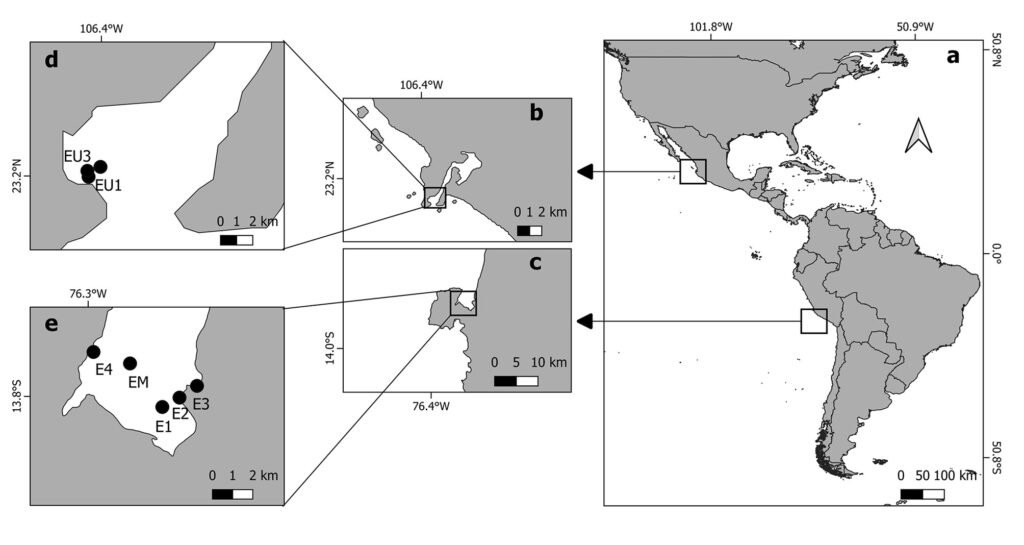
Figure 1. a, Map of the study sites; b, d, sampling sites in Estero de Urías (EU1, EU2, EU3), Mexico; c, e, Paracas Bay (E1, E2, E3, E4, EM), Peru.
Paracas Bay (PB; 13.8° S) is located in Pisco, off South-Central Peru (Fig. 1), with an area of 30 km2 and < 15 m of depth (Merma-Mora et al., 2024). The southern part of the bay is included in the Paracas National Reserve (Sernanp, 2019). It is influenced by one of the main upwelling cells of the highly productive Peruvian Upwelling System (Chávez et al., 2008). PB is seasonally influenced by river discharge, and monthly averages range from 0.7 to 282 m3 s−1, with the higher values in austral summer (Cuellar-Martinez et al., 2023).
The climate in the region is arid, with an average annual rainfall of 1.83 mm and air temperatures ranging from 15 to 22 °C (Reyes, 2009). Anthropogenic activities around the bay include artisanal and industrial fishing, tourism, bay scallop Argopecten purpuratus aquaculture, fish processing industries, non-metallic minerals, and guano extraction (Reyes, 2009). The Terminal Portuario General San Martín, the country’s third most important port for cargo traffic (APN, 2018), is in the surroundings.
The most abundant macrophytes were collected manually or by diving and placed in polypropylene bags; the macrophyte masses ranged from 5 to 342.2 g in wet weight. The 3 sampling sites at EUL were close to the lagoon mouth, where a greater diversity of macroalgae species is found (Ochoa-Izaguirre et al., 2002). The sites were located in a total area of 0.01 km2 with fish cage cultures (~ 8 m depth). The most abundant macroalgae attached to the floating cage frames were collected monthly between August and November 2018 and in January, February, April, and June 2019. A total of 25 samples were collected, including species of Gracilaria sp., Hynea sp., Sargassum sp., Padina sp., Grateloupia sp., and Gelidium sp. In general, 1 to 4 samples were collected per sampling station. In addition, between August and October 2018, artificial substrates consisting of rectangular pieces (3 x 33 cm) of fiberglass screen fixed on a rigid frame were used (Jauzein et al., 2016). The artificial substrates were collected using scissors. For retrieval, 24 hours after installation, the substrate was cut on one side and carefully placed into a plastic bottle filled with 250 ml of ambient seawater. Then, the other side of the substrate was cut and placed inside the bottle, which was capped underwater (Jauzein et al., 2016).
In PB, the most abundant macrophytes, such as Caulerpa filiformis, Chondracanthus chamissoi, and Ruppia maritima were collected at 5 sites during June and November 2021, and April 2022. The sites were shallow (~ 1 m depth), whereas E1 and EM were 5 m and 10 m deep, respectively. A total of 24 samples were obtained. Additionally, surface water was sampled daily in E1 to evaluate the presence of EDs in the water (cells L-1), and HOBO data loggers (Onset UA-001-64) recorded surface and bottom temperatures every 20 minutes.
Environmental parameters (temperature, salinity, dissolved oxygen, and chlorophyll a) were measured in both PB and EUL using EXO (YSI) multiparameter sondes. In EUL, the chlorophyll a sensor was calibrated using rhodamine standards according to the manufacture’s guidelines (YSI Inc., 2014), allowing chlorophyll a concentrations to be expressed in absolute units (μg L⁻¹). In contrast, no calibration was performed in PB; thus, chlorophyll a values are reported in RFU (relative fluorescence units), reflecting the raw sensor response. Although not directly comparable to absolute concentrations, RFU values are widely used to identify temporal patterns in relative chlorophyll a concentrations (Foster et al., 2022). In the EUL, measurements were taken near the sampling sites (1-2 km) at stations 3 and 4 for the coastal observatory of global change in Mazatlán (Fig. 1 in Sanchez-Cabeza et al., 2019) and at station E1 for PB.
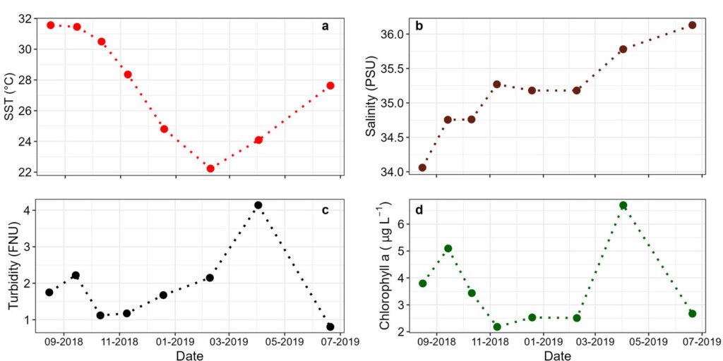
Figure 2. Mean values of the sea surface temperature (SST in °C). a) Salinity (PSU; b), turbidity (in nephelometric turbidity units, NTU); c) chlorophyll a concentration (in µg L-1; d) in the Estero de Urías Lagoon, at the entrance of the Gulf of California.
In the laboratory, the bags with macrophytes and bottles with artificial substrates were vigorously agitated for 2 minutes. The suspension was filtered through sieves with 250 µm, 150 µm, and 20 µm mesh to remove larger particles. The fraction retained in the 20 µm sieve was concentrated and transferred to a vial of 50 ml filled with seawater filtered through Whatman GF/F filters (nominal pore size ~ 0.7 µm), and preserved with 1% acidic Lugol’s iodine fixative. The EDs counting was performed on 3 replicate subsamples from the same macrophyte sample, using a Sedgwick-Rafter chamber in an optical microscope (LM Leica DMR, Wetzlar, Germany) with 200× magnification. Cell abundances were reported as cells per g w.w. of macrophyte (Reguera et al., 2011). The reported uncertainty is the standard deviation of the mean of 3 replicate counts.
The Shapiro test confirmed that species densities were not normally distributed. Therefore, Kruskal-Wallis one-way ANOVA and Dunn’s multiple comparison post hoc tests were used to assess whether abundances and environmental variables exhibited significant variations during the study period. The significance level (α) was set at < 0.05. All analyses and plots were performed with R version 2024.04.2 (R Core Team, 2024).
Results
Estero de Urías Lagoon
During the study period, the sea surface temperature (SST) varied from 22.2 to 31.6 °C, salinity from 34.0 to 36.1, turbidity from 0.8 to 4.1 NTU, and chlorophyll a from 2.2 to 6.7 mg L-1. The highest SST was observed in August-September, 2018 (Fig. 2).
No EDs were observed attached to the artificial substrates in the EUL. Macroalgae were not found in EU2 in November 2018 and June 2019. Dinoflagellates on the EUL macroalgae belonged to the genus Prorocentrum; the highest abundances corresponded to P. micans (Supplementary material; Fig. S1). Prorocentrum lima complex was frequently observed in the samples, with abundances ranging from 0 to 78±45 cells g-1. No significant differences in the abundances were observed between seasons or among stations (Fig. 3a, b). Spearman’s correlation between the abundances of EDs and environmental variables was not significant.
Paracas Bay
During the study period, temperatures were from 14.1 to 22.2 °C. The sea surface and bottom temperatures were significantly higher in autumn (surface temperatures: 18.0-22.2 °C; bottom temperatures: 17.5-21.6 °C) than in summer and spring (surface temperatures: 14.5-22.1 °C; bottom temperatures: 14.1-19.7 °C; Fig. 4a). In the 3 seasons, the surface temperatures were significantly higher than the bottom temperatures. When the P. lima complex was observed in the water column and associated with macrophytes (May 14-Jun 04), SST ranged from 18.0 to 22.2 °C. Chlorophyll a ranged from 0.45 to 7.12 RFU. The highest values were observed in autumn, while spring and summer values were similar. The salinity varied between 34.4 and 35.2, with higher values in autumn than in spring and summer (4b).
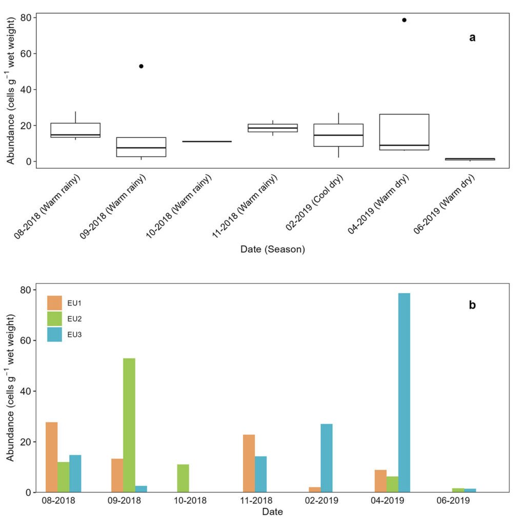
Figure 3. a) Abundance of the Prorocentrum lima complex, with seasons indicated in parentheses. Boxplots show the median (horizontal line), the interquartile range (the difference between the third and first quartile; box). Whiskers extend to values within 1.5 times the interquartile range, and data beyond this range are shown as outliers (dots); b, total abundance by station sites in the Estero de Urías Lagoon, located at the entrance of the Gulf of California.
In Paracas Bay, EDs were absent during most of the study period, and the P. lima complex was detected only in the austral autumn (June 2-4, 2021; Fig. 5, Table 1) with the highest abundances (867±172 cells g-1 in station E3). The P. lima complex was attached mostly to C. filiformis (Table 1).
According to the high-frequency monitoring of Prorocentrum species in surface water, P. micans was a common dinoflagellate in austral autumn and summer, and its abundances were from 40 to 1,840 cells L-1 (Supplementary material; Fig. S2). The P. lima complex was observed only in the austral autumn with a maximum abundance (1,360 cell L-1) on May 14, and between May 17 and June 01, its abundances were ≤ 280 cells L-1 (Fig. 4c).
Discussion
Artificial substrates have been successfully used for quantifying and monitoring EDs, particularly in sheltered, shallow, and subtidal sites (Tester et al., 2022). The lack of EDs attached to the artificial substrates in EUL is likely related to the low abundance of these organisms and the lagoon’s turbulent hydrodynamics. Low abundances of EDs were also observed associated with macroalgae. These results agree with observations from the coast of Tonga in an area exposed to high wave action, where Argyle (2018) detected low abundances of Gambierdiscus cells in association with macrophytes, but the artificial substrate failed to collect them. In contrast, Gambierdiscus concentrations were high on natural and artificial substrates deployed at sheltered, shallow, and subtidal sites. Despite EUL mouth having the highest macroalgae diversity (Ochoa-Izaguirre et al., 2002), it is not a sheltered zone. It is influenced by the tidal regime since the energy available for water circulation is primarily provided by tidal pumping, with tidal velocities of up to 0.60 m s-1 at the main channel (Montaño-Ley et al., 2008). The EDs can be attached by coating mucus or can live freely within the macroalgae interstices, so the turbulence and currents make them vulnerable to cell dispersal. They are mainly found in areas with low to moderately low energy environments (Foden et al., 2005).
Table 1
Abundance of Prorocentrum species in Paracas Bay in the austral autumn.
| Species | Date | Season | Station | Macrophyte species | Abundance (cells g wet weight)* |
| Prorocentrum lima complex | 2021-06-02 | Autumn | E3 | Caulerpa filiformis | 861±172 |
| Prorocentrum lima complex | 2021-06-02 | Autumn | E3 | Caulerpa filiformis | 250±17 |
| Prorocentrum lima complex | 2021-06-02 | Autumn | E3 | Caulerpa filiformis | 13±3 |
| Prorocentrum micans | 2021-06-02 | Autumn | E3 | Caulerpa filiformis | 6±5 |
| Prorocentrum lima complex | 2021-06-04 | Autumn | E3 | Chondracanthus chamissoi +Ulva sp. | 0 |
| Prorocentrum lima complex | 2021-06-04 | Autumn | E3 | Red algae | 0 |
| Prorocentrum lima complex | 2021-06-04 | Autumn | E3 | Red algae | 0 |
| Prorocentrum lima complex | 2021-06-04 | Autumn | E4 | Chondracanthus chamissoi | 1±1 |
| Prorocentrum lima complex | 2021-06-04 | Autumn | E4 | Ruppia marítima | 5±5 |
| Prorocentrum lima complex | 2021-06-04 | Autumn | E4 | Ruppia maritima | 5±2 |
* Abundances represent the average of 3 independent counts performed on the same sample. Values are reported as the mean ± standard deviation.
Among the Prorocentrum species associated with macrophytes in this study, only P. lima complex is recognized as a benthic species (Okolodkov et al., 2022), and it is the first time that P. lima complexis reportedattached to macrophytes in EUL and PB. This cosmopolitan taxon is widely distributed in South America (Mafra et al., 2023). Although low abundances were observed in PB, P. lima has been recorded in the water column with abundances of up to 4.5×10⁴ cells L-1 (Cuellar-Martinez et al., 2023). Caulerpa filiformis is the most representative species in the macroalgae assemblage of PB (Olivas-Valverde, 2013), and the highest abundances of P. lima complex were observed on this species. Although information about the toxicity of P. lima complex is not available in strains from PB or EUL, reports worldwide reveal that all studied P. lima strains produce toxins related to DSP, such as okadaic acid, and several strains produce dinophysistoxins-1 (DTX1; Nishimura et al., 2020). Thus, monitoring this species on different substrates is relevant.
The presence of P. lima complex in both the water column and on macroalgae in Paracas Bay coincided with the highest temperatures recorded during the study period. Aissaoui et al. (2014) mentioned that this species appears to be eurythermal and euryhaline, as it grows over a wide interval of temperatures and salinities. In this work, P. lima complex was observed over a wide range of temperatures (18.0-31.6 °C), suggesting a remarkable ecological plasticity and ability to colonize diverse niches. Although P. lima complex was previously observed in PB at temperatures ranging from 15 to 25 °C (Mafra et al., 2023), in this study it was detected during autumn, when the highest temperatures reached 17.5-22.2 °C. Aquino-Cruz et al. (2018) highlighted the importance of temperature on cell growth rates, toxin levels, and photosynthetic efficiency. They determined that the optimum growth of P. lima strains from the United Kingdom occurred at 15-25 °C, with an increment in the production of okadaic acid at 15 °C.
Temperatures also affect the range of species distribution. It is expected that warmer temperatures associated with climate change could benefit harmful benthic dinoflagellate species, expanding their geographical distribution range (Tester et al., 2020). Another factor associated with distribution expansion is the artificial introduction of discharged ballast ship water (Park et al., 2021). The sampling period of this study limits the potential for making strong extrapolations regarding the temporal dynamics of the DEs and their ecological dynamics. Nevertheless, the detection of DEs with potential toxin production is a relevant finding that highlights the need for longer-term monitoring to better understand their ecological dynamics and potential harmful implications for environmental health and human activities.
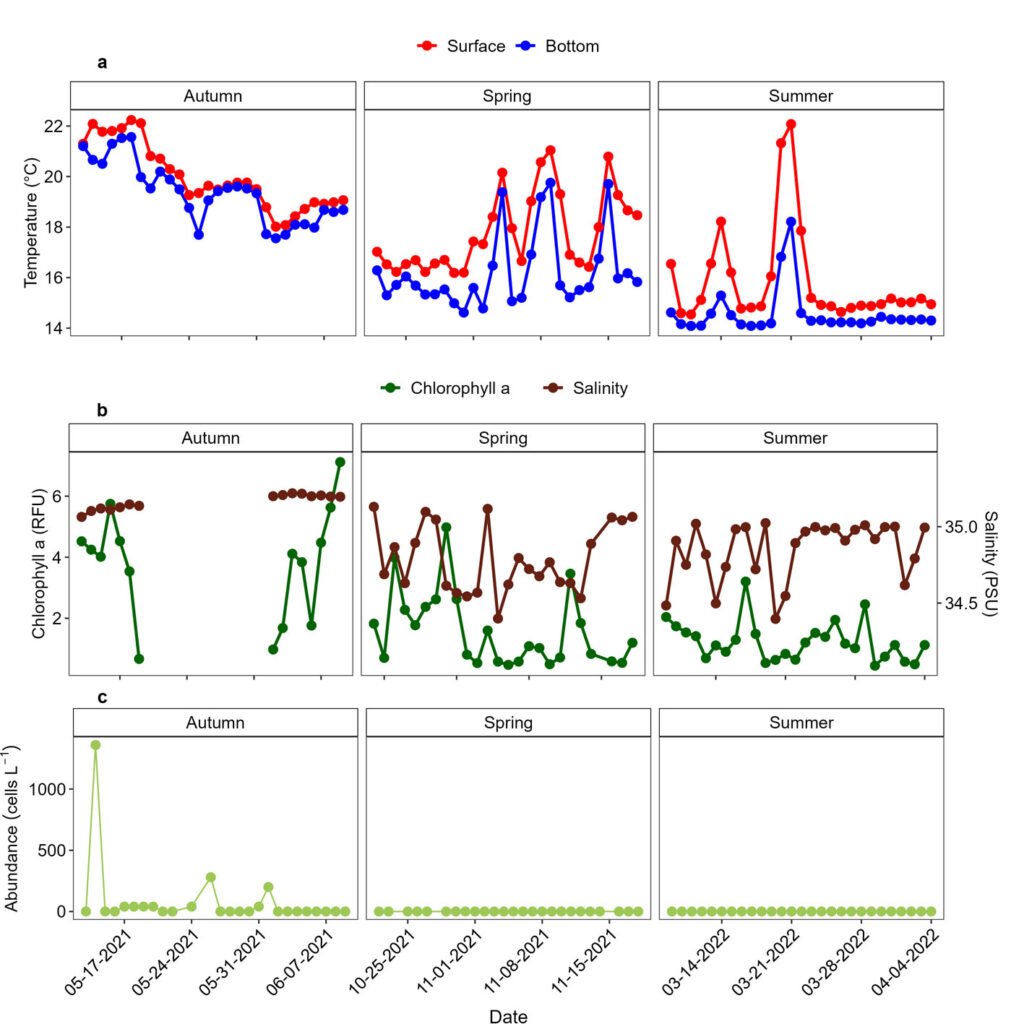
Figure 4. Surface and bottom temperatures (in °C). a) Surface salinity (PSU) and chlorophyll a (in relative fluorescence units, RFU; b), and seasonal abundances of Prorocentrum lima complex in surface waters (c) at the E1 station in Paracas Bay, Peru.
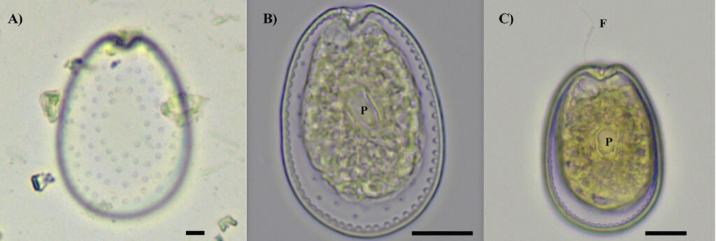
Figure 5. Vegetative cells of Prorocentrum lima complex collected from Paracas Bay, Peru, observed under light microscopy. A) Surface focus on a vegetative cell showing the pore pattern, B) cell showing pyrenoid (P), C) cell showing pyrenoid and flagellu. Scale bar: 10 µm.
The epibenthic dinoflagellate community was explored at 2 sites influenced by upwellings: Estero de Urías Lagoon, at the entrance to the Gulf of California, and Paracas Bay, off south-central Peru. The Prorocentrum lima complex was commonly found with low abundances, mainly associated with macrophytes in Estero de Urías Lagoon and sporadically detected in Paracas Bay (mainly on Caulerpa filiformis). In the water column of Paracas Bay, the P. lima complex was observed during the period with the highest recorded temperature in the study, suggesting potential environmental influences. These initial findings highlight the need for long-term studies with higher temporal resolution and increased detection frequency to better understand the environmental relationships of the benthic dinoflagellate at the studied sites. Given the known production of diarrhetic shellfish toxins by P. lima, its possible sensitivity to climate-related changes, and the anthropogenic pressures present in both study areas —such as intense marine traffic— further monitoring and multidisciplinary research, including toxicological, physiological, and molecular studies, are strongly recommended to assess the potential risks posed by P. lima to marine ecosystems and public health.
Acknowledgments
This work was supported by UNAM ICML (#347), IAEA-RLA/7014 and 7028, Project Concytec – World Bank 05-2019-FONDECYT-BM. This is a contribution to the Marine-Coastal Research Stressors Network for Latin America and the Caribbean (REMARCO) www.remarco.org and to the IRN DEXICOTROP of the Institut de Recherche pour le Développement (IRD). The authors thank M. Rangel, O. López Ramos, M. Fregoso-López, B. Yáñez-Chávez, H. Bojórquez-Leyva, and F. Rioual for the help provided in the fieldwork; R. Alonso-Rodríguez, J. A. Cabello Coral, B. Yáñez-Rivera, for microscopy facilities. F. Ramos-Huamaní and L. H. Pérez-Bernal for the laboratory analyses, and M. Ochoa-Izaguirre for the identification of macroalgae from the Estero de Urías Lagoon.
References
Aissaoui, A., Armi, Z., Akrout, F., & Ben-Hassine, O. K. (2014). Environmental factors and seasonal dynamics of Prorocentrum lima population in coastal waters of the Gulf of Tunis, South Mediterranean. Water Environment Research, 86, 2256–2270. https://doi-org/2443/10.2175/106143014X13975035526266
Álvarez, E. A., Klemm, K., Hoppenrath, M., Cembella, A., John, U., & Karlson, B. (2022). Temporal and spatial distribution of epibenthic dinoflagellates in the Kattegat-Skagerrak, NE Atlantic-Focus on Prorocentrum lima and Coolia monotis. Harmful Algae, 118, 102318. https://doi.org/10.1016/j.hal.2022.102318
API (Administración Portuaria Integral). (2024). Puerto de Mazatlán: plataforma logística integral. Available at https://www.puertomazatlan.com.mx/APIWEB/PRESENTA
TION_APIMAZ.PDF (Accessed May 20 2024).
APN (Autoridad Portuaria Nacional). (2018). Plan Maestro del Terminal Portuario General San Martin. Lima, Peru. Available at: http://webaplicacion.apn.gob.pe/proyecto/wp-
content/uploads/2020/10/Plan-Maestro-Portuario-TP-GENERAL-SAN-MARTIN.pdf (Accessed: March 11, 2024).
Aquino-Cruz, A., Purdie, D. A., & Morris, S. (2018). Effect of increasing sea water temperature on the growth and toxin production of the benthic dinoflagellate Prorocentrum lima. Hydrobiologia, 813, 103–122. https://doi.org/10.1007/s10750-018-3512-4
Argyle, P. A. (2018). The ecology and toxin production of Gambierdiscus and Fukuyoa species from the Pacific (Ph.D. Thesis). University of Canterbury, New Zealand.
Berdalet, E., Fleming, L. E., Gowen, R., Davidson, K., Hess, P., Backer et al. (2016). Marine harmful algal blooms, human health and wellbeing: challenges and opportunities in the 21st century. Journal of the Marine Biological Association of the United Kingdom, 96, 61–91. https://doi.org/10.1017/S0025315415001733
Cardoso-Mohedano, J. G., Lima-Rego, J., Sanchez-Cabeza, J. A., Ruiz-Fernández, A. C., Canales-Delgadillo, J., Sánchez-Flores, E. I. et al. (2018). Sub-tropical coastal lagoon salinization associated to shrimp ponds effluents. Estuarine, Coastal and Shelf Science, 203, 72–79. https://doi.org/10.1016/j.ecss.2018.01.022
Chávez, F. P., Bertrand, A., Guevara-Carrasco, R., Soler, P., & Csirke, J. (2008). The northern Humboldt Current System: Brief history, present status and a view towards
the future. Progress in Oceanography, 79, 95–105. https://doi.org/10.1016/j.pocean.2008.10.012
Chinain, M., Gatti, C. M. I., Darius, H. T., Quod, J. P., & Tester, P. A. (2021). Ciguatera poisonings: A global review of occurrences and trends. Harmful Algae, 102, 101873. https://doi.org/10.1016/j.hal.2020.101873
Cuellar-Martinez, T., Ochoa, A. D. R. H., Sánchez, S., Aguirre-Velarde, A., Ocas, E. O. M., Velasquez, A. M. R. et al. (2023). Abundance and distribution of potentially toxic phytoplankton in aquaculture sites along the Peruvian coast. Journal of Marine Systems, 240, 103865. https://doi.org/10.1016/j.jmarsys.2023.103865
do Prado-Leite, I., Menegotto, A., da Cunha-Lana, P., & Júnior, L. L. M. (2022). A new look at the potential role of marine plastic debris as a global vector of toxic benthic algae. Science of the Total Environment, 838, 156262. https://doi.org/10.1016/j.scitotenv.2022.156262
Durán-Riveroll, L. M., Cembella, A. D., & Okolodkov, Y. B. (2019). A review on the biodiversity and biogeography of toxigenic benthic marine dinoflagellates of the coasts of Latin America. Frontiers in Marine Science, 6, 148. https://doi.org/10.3389/fmars.2019.00148
Foden, J., Purdie, D. A., Morris, S., & Nascimento, S. (2005). Epiphytic abundance and toxicity of Prorocentrum lima populations in the Fleet Lagoon, UK. Harmful Algae, 4, 1063–1074. https://doi.org/10.1016/j.hal.2005.03.004
Foster, G. M., Graham, J. L., Bergamaschi, B. A., Carpenter, K. D., Downing, B. D., Pellerin, B. A. et al. (2022). Field techniques for the determination of algal pigment fluorescence in environmental waters. Principles and guidelines for instrument and sensor selection, operation, quality assurance, and data reporting (No. 1-D10). Virginia: US Geological Survey. https://doi.org/10.3133/tm1D10
Gobler, C. J., Doherty, O. M., Hattenrath-Lehmann, T. K., Griffith, A. W., Kang, Y., & Litaker, R. W. (2017). Ocean warming since 1982 has expanded the niche of toxic algal blooms in the North Atlantic and North Pacific oceans. Proceedings of the National Academy of Sciences, 114, 4975–4980. https://doi.org/10.1073/pnas.1619575114
Hernández-Cornejo, R., & Ruiz-Luna, A. (2000). Development of shrimp farming in the coastal zone of southern Sinaloa (Mexico): operating characteristics, environmental issues, and perspectives. Ocean & Coastal Management, 43, 597–607. https://doi.org/10.1016/S0964-5691(00)00049-1
Herrera-Becerril, C. A., Sanchez-Cabeza, J. A., Sánchez, L. F. Á., Lara-Cera, A. R., Ruiz-Fernández, A. C., Cardoso-Mohedano, J. G. et al. (2022). Statistical identification of coastal hypoxia events controlled by wind-induced upwelling. Continental Shelf Research, 233, 104634. https://doi.org/10.1016/j.csr.2021.104634
Honsell, G., Bonifacio, A., De Bortoli, M., Penna, A., Battocchi, C., Ciminiello, P. et al. (2013). New insights on cytological and metabolic features of Ostreopsis cf. ovata Fukuyo (Dinophyceae): A multidisciplinary approach. Plos One, 8, e57291. https://doi.org/10.1371/journal.pone.0057291
Jauzein, C., Fricke, A., Mangialajo, L., & Lemée, R. (2016). Sampling of Ostreopsis cf. ovata using artificial substrates: optimization of methods for the monitoring of benthic harmful algal blooms. Marine Pollution Bulletin, 107, 300–304. https://doi.org/10.1016/j.marpolbul.2016.03.047
Lee, E. S., Hwang, J., Hyung, J. H., & Park, J. (2021). Detection of the benthic dinoflagellates, Ostreopsis cf. ovata and Amphidinium massartii (Dinophyceae), Using Loop-Mediated Isothermal Amplification. Journal of Marine Science and Engineering, 9, 885. https://doi.org/10.3390/jmse9080885
Mafra, Jr., L. L., Sunesen, I., Pires, E., Nascimento, S. M., Álvarez, G., Mancera-Pineda, J. E. et al. (2023). Benthic harmful microalgae and their impacts in South America. Harmful Algae, 127, 102478. https://doi.org/10.1016/j.hal.2023.102478
Méndez, N. (2002). Annelid assemblages in soft bottoms subjected to human impact in the Urías Estuary (Sinaloa, Mexico). Oceanologica Acta, 25, 139–147. https://doi.org/
10.1016/S0399-1784(02)01193-3
Merma-Mora, L., Colas, F., Cardich, J., Sánchez, S., Flores, E., Lorenzo, A. et al. (2024). Bottom-water hypoxia in the Paracas Bay (Peru, 13.8° S) associated with seasonal and synoptic time scale variability of winds and water stratification. Journal of Marine Systems, 241, 103918. https://doi.org/10.1016/j.jmarsys.2023.103918
Montaño-Ley, Y., Peraza-Vizcarra, R., & Páez-Osuna, F. (2008). Tidal hydrodynamics and their implications for the dispersion of effluents in Mazatlán Harbor: An urbanized shallow coastal lagoon. Water, Air, and Soil Pollution, 194, 343–357. http://dx.doi.org/10.1007/s11270-008-9721-0
Nishimura, T., Uchida, H., Noguchi, R., Oikawa, H., Suzuki, T., Funaki, H. et al. (2020). Abundance of the benthic dinoflagellate Prorocentrum and the diversity, distribution, and diarrhetic shellfish toxin production of Prorocentrum lima complex and P. caipirignum in Japan. Harmful Algae, 96, 101687. https://doi.org/10.1016/j.hal.2019.101687
Ochoa-Izaguirre, M. J., Carballo, J. L., & Páez-Osuna, F. (2002). Qualitative changes in macroalgal assemblages under two contrasting climatic conditions in a subtropical estuary. Botanica Marina, 45, 130–138. https://doi.org/10.1515/BOT.2002.014
Okolodkov, Y. B., Durán-Riveroll, L. M., Band-Schmidt, C. J., Leyva-Valencia, I., Gárate-Lizárraga, I., & Cembella, A. D. (2022). A review on marine benthic dinoflagellates in Mexico. Hidrobiológica, 32, 183–210. https://doi.org/10.24275/uam/izt/dcbs/hidro/2022v32n3/okolodkov
Olivas-Valverde, J. A. (2013). Informe de evaluación e identificación de potenciales riesgos ambientales en flora y fauna en la Bahía de Paracas, provincia de Pisco, departamento de Ica. Organismo de Evaluación y Fiscalización Ambiental. Gobierno de Perú. Available at https://repositorio.oefa.gob.pe/handle/20.500.12788/1214 (Accessed May 28, 2024).
Park, J. S., Li, Z., Kim, H. J., Kim, K. H., Lee, K. W., Youn, J. Y. et al. (2021). First report of the marine benthic dinoflagellate Bysmatrum subsalsum from Korean tidal pools. Journal of Marine Science and Engineering, 9, 649. https://doi.org/10.3390/jmse9060649
Raygoza-Viera, J. R., Ruiz-Fernández, A. C., Ruelas-Inzunza, J., Alonso-Hernández, C., Pérez-Bernal, L. H., & Páez-Osuna, F. (2014). Accumulation and distribution of Hg and 210Pb in superficial sediments from a coastal lagoon in the SE Gulf of California associated with urban-industrial and port activities. Environmental Earth Sciences, 72, 2729–2739. https://doi.org/10.1007/s12665-014-3178-9
R Core Team. (2024). R: a language and environment for statistical computing. R Foundation for Statistical Computing, Vienna, Austria. https://www.R-project.org/
Reguera, B., Alonso, R., Moreira, A., & Méndez, S. (2011). Guía para el diseño y puesta en marcha de un plan de seguimiento de microalgas productoras de toxinas. Proyecto ARCAL RLA 7/014. París, Viena: UNESCO/ OIEA.
Reyes, J. (2009). Paracas, nuestra Reserva. Información básica sobre la Reserva Nacional de Paracas (2ª ed.). Áreas Costeras y Recursos Marinos, [ACOREMA]. http://humboldt.iwlearn.org/es/sitios-piloto/-1/paracas.pdf
Sanchez-Cabeza, J. A., Álvarez Sánchez, L. F., Cardoso-Mohedano, J. G., Escalante-Mancera, E., Díaz-Asencio, M., López-Rosas, H. et al. (2019). A low-cost long-term model of coastal observatories of global change. Journal of Operational Oceanography, 12, 34–46. https://doi.org/10.1080/1755876X.2018.1533723
Sernanp (Servicio Nacional de Áreas Naturales Protegidas). (2019). Reserva Nacional de Paracas. Servicio Nacional de Áreas Naturales Protegidas por el Estado. Available at: https://www.gob.pe/institucion/sernanp/informes-publicaciones/1718991-reserva-nacional-de-paracas (Accessed October 23, 2024).
SMN (Servicio Meteorológico Nacional). (2024). Normales climatológicas Mazatlán 1951-2017. Available at https://smn.cna.gob.mx/tools/RESOURCES/Diarios/25062.txt
Tester, P. A., Feldman, R. L., Nau, A. W., Kibler, S. R., & Litaker, R. W. (2010). Ciguatera fish poisoning and sea surface temperatures in the Caribbean Sea and the West Indies. Toxicon, 56, 698–710. https://doi.org/10.1016/j.toxicon.2010.02.026
Tester, P. A., Litaker, R. W., & Berdalet, E. (2020). Climate change and harmful benthic microalgae. Harmful Algae, 91, 101655. https://doi.org/10.1016/j.hal.2019.101655
Tester, P. A., Litaker, R. W., Soler-Onís, E., Fernández-Zabala, J., & Berdalet, E. (2022). Using artificial substrates to quantify Gambierdiscus and other toxic benthic dinoflagellates for monitoring purposes. Harmful Algae, 120, 102351. https://doi.org/10.1016/j.hal.2022.102351
Yong, H. L., Mustapa, N. I., Lee, L. K., Lim, Z. F., Tan, T. H., Usup, G. et al. (2018). Habitat complexity affects benthic harmful dinoflagellate assemblages in the fringing reef of Rawa Island, Malaysia. Harmful Algae, 78, 56–68. https://doi.org/10.1016/j.hal.2018.07.009
YSI Inc. (2014). EXO Rhodamine WT Smart Sensor Calibration Guide. Available at: https://www.fondriest.com/pdf/ysi_exo_rhodamine_cal.pdf

Vascular epiphyte community of an inland mangrove of Tabasco: composition and similarity with coastal mangroves and adjacent tropical vegetation
Vascular epiphyte community of an inland mangrove of Tabasco: composition and similarity with coastal mangroves and adjacent tropical vegetation
Comunidad epífita vascular de un manglar interior de Tabasco: composición y similitud con manglares costeros y vegetación tropical adyacente
Neil Ebeth Meled Morales-Rodríguez a, *, Carlos Manuel Burelo-Ramos a, José G. García-Franco b, Octavio Aburto-Oropeza c y María Eugenia Molina-Paniagua a
a Universidad Juárez Autónoma de Tabasco, Laboratorio de Manglares Interiores, Carretera Villahermosa-Cárdenas Km. 0.5 s/n, Entronque a Bosques de Saloya, 86150 Villahermosa, Tabasco, Mexico
b Instituto de Ecología, Carretera antigua a Coatepec #351, Col. El Haya, 91073 Xalapa, Veracruz, Mexico
c Scripps Institution of Oceanography, 9500 Gilman Drive, La Jolla, California 92093, USA
*Corresponding author: nemmr@hotmail.com (N.E.M. Morales-Rodríguez)
Received: 13 December 2024; accepted: 23 October 2025
Abstract
El Cacahuate Lagoon, Tabasco, Mexico, is located 170 km from the current coastline and contains an inland mangrove ecosystem, surrounded by remnants of tropical forest. This inland mangrove is the habitat of an epiphyte community whose species composition and relationship with other epiphyte communities are unknown. This study describes the composition of vascular epiphytes associated with this inland mangrove, evaluates their similarity to epiphyte communities in coastal mangroves and adjacent vegetation within a 220 km radius of the study site, using the Jaccard Index and floristic turnover with β-diversity. We hypothesize that the similarity in the composition of the epiphytes of the inland mangrove should be greater with that of nearby forests than with coastal mangroves, since the seeds of forest epiphytes can easily reach the inland mangrove. The epiphyte community of the Cacahuate mangrove comprises 27 species and is more similar to the epiphyte communities of the coastal mangroves of Tabasco. This affinity could be related to the Pleistocene isolation of this mangrove, or to the long-distance dispersal of epiphytes from coastal mangroves.
Keywords: Biodiversity; Floristics; Red mangrove; Rhizophora mangle; Wanha’ Biosphere Reserve
Resumen
La laguna El Cacahuate, Tabasco, México, se localiza a 170 km de la línea costera actual y contiene un ecosistema de manglar interior, rodeado de remanentes de bosque tropical. Este manglar interior es el hábitat de una comunidad epífita cuya composición de especies y su relación con otras comunidades epífitas se desconocen. El presente estudio describe la composición de epífitas vasculares asociadas con este manglar interior, evalúa su similitud con las comunidades epífitas de los manglares costeros y vegetación adyacente en un radio de 220 km del lugar de estudio, utilizando el índice de Jaccard y su recambio florístico con la diversidad ß. Hipotetizamos que la similitud en la composición de las epífitas del manglar interior debería ser mayor con la de los bosques cercanos que con los manglares costeros, ya que las semillas de las epífitas de los bosques pueden llegar fácilmente al manglar interior. La comunidad epífita del manglar del Cacahuate comprende 27 especies y presenta una mayor similitud con las comunidades epífitas de los manglares costeros de Tabasco. Esta afinidad podría estar relacionada con el aislamiento pleistocénico de este manglar, o con la dispersión a larga distancia de las epífitas provenientes de los manglares costeros.
Palabras clave: Biodiversidad; Florística; Mangle rojo; Rhizophora mangle; Reserva de la Biosfera Wanha’
Introduction
Vascular epiphytic plants (henceforth epiphytes) constitute a functional group that develops on woody species. Unlike parasitic plants, epiphytes obtain water and nutrients from the atmosphere, precipitation, and decomposing organic material, rather than relying physiologically on the host (Krömer & Gradstein, 2016). Within epiphytes, 2 main categories are recognized: true epiphytes, which complete their entire life cycle on the host without producing roots that reach the soil, and hemiepiphytes, which in contrast, exhibit a mixed life cycle, since some germinate on the host and later develop roots that reach the ground (primary hemiepiphytes), whereas others begin their growth in the soil and, as they ascend, establish themselves on the host (secondary hemiepiphytes) (Granados-Sánchez et al., 2003; Zotz, 2016). Epiphytes comprise about 10% of the known plant species worldwide (Zotz et al., 2021). In the Neotropics, epiphytes significantly contribute to the overall diversity of the vegetation, as they can represent up to 50% of the vascular flora in some forests (Carmona-Higuita et al., 2025; Kelly et al., 2004; Taylor et al., 1986). Tree species in the low and mountain forests have different structural characteristics (e.g., greater height, dense canopy, and great diversity of bark textures), which combined with particular environmental conditions (e.g., high humidity), allow the presence of a high number of epiphytic species (Ceja-Romero et al., 2008; Flores-Palacios & García-Franco, 2006; Hietz & Hietz, 1995; Krömer et al., 2007, 2014; Martínez-Meléndez et al., 2011; Rzedowski, 1996). In contrast, mangrove forests generally show a low richness of epiphytes (Benzing, 1990; Carmona-Díaz et al., 2014; Zotz & Reuter, 2009; Zimmerman & Olmsted, 1992), which can be attributed to reduced tree diversity and consequently to low structural complexity of the habitat, but mainly due to environmental stress conditions such as the strong winds, waves, and high salinity present in coastal zones (Gómez & Winker, 1991; Jiménez-López et al., 2017; Zotz & Reuter, 2009). However, epiphytes are frequent in mangrove ecosystems, as several species have been recorded in different studies even though the objectives and sampling efforts are directed toward tree species, which are the dominant physiognomic elements (Aksornkoae, 1993; Cach-Pérez et al., 2013; Carmona-Díaz et al., 2014; De Sousa & Colpo, 2017; García-Luna et al 2024; Jiménez-López et al., 2018; Kupec, 2018; Noguera-Savelli et al., 2021; Rahman et al., 2015; Rohani et al., 2020).
Mangrove ecosystems are primarily distributed in tropical and subtropical regions, generally associated with the coast and brackish water bodies (Leal & Spalding, 2021). However, mangrove ecosystems also have been recorded in freshwater wetlands, away from marine influence, known as inland mangroves. The inland mangroves have been reported in many countries worldwide, such as in Australia, Antigua and Barbuda, the Bahamas, Indonesia, and Pakistan, located 15 to 50 km from the coast, and between 6 and 37 m above sea level (Lugo, 1981; Patel, 2014; Patel & Agoramoorthy, 2012; Stoddart et al., 1973; Taylor, 1986; Tripathi et al., 2013; Woodroffe, 1988).
Recently, in Mexico, individuals of Rhizophora mangle, along with another 112 coastal affinity species were reported along the banks of the San Pedro Mártir River and El Cacahuate Lagoon in Tabasco, the latter located almost on the border with Guatemala (Aburto-Oropeza et al., 2021). The presence of this inland mangrove is attributed to the global climatic phenomenon that occurred about 120,000 years ago when an increase in global temperatures caused a rise in sea levels, displacing the coastline inland (Aburto-Oropeza et al., 2021). As the planet cooled, the sea retreated to its current position, leaving mangrove trees dispersed along the riverbanks and creating an isolated mangrove ecosystem in the El Cacahuate Lagoon, 170 km from the Tabasco coast (Aburto-Oropeza et al., 2021).
Currently, the El Cacahuate Lagoon is surrounded by a matrix composed of remnants of evergreen tropical forest belonging to the “Cañón del Usumacinta” Flora and Fauna Protection Zone (Conanp, 2015), fragments of several types of tropical forest, and large areas of land used for livestock and agriculture activities. However, despite this mixed landscape, the hydrophytic vegetation surrounding the water body restricts access to the mangrove, which has resulted in minimal human impact. El Cacahuate mangrove is considered a relict area from the Pleistocene and a refuge for biodiversity due to its high degree of conservation (Aburto-Oropeza et al., 2021). This area together with the adjacent forest areas forms part of a core area of the recently designated Wanha’ Biosphere Reserve (Conanp, 2023a; Semarnat, 2023).
Preliminary surveys indicate the presence of several species of epiphytes along the upper San Pedro River (Aburto-Oropeza et al., 2021). However, in El Cacahuate mangrove the epiphyte species composition and its species similarities to the epiphytic communities of the surrounding vegetation or to the coastal mangroves of Gulf of Mexico are unknown. High epiphyte composition similarity with tropical forest would indicate processes of colonization after the sea retired, while high epiphyte composition with coastal mangroves communities should indicate that species arrived together with the mangrove during the interglacial period.
The aims of this study were to determine the richness and composition of the epiphyte community present in the inland mangrove of El Cacahuate Lagoon, and to assess the floristic similarity of the epiphytes of El Cacahuate with coastal mangroves and adjacent tropical forests. We expect that, given the inland Cacahuate mangrove’s location in a freshwater environment and its proximity to tropical forest areas, the similarity of the epiphyte community should be greater than that of the nearest terrestrial vegetation because the seeds of the epiphytes can likely reach the mangrove trees easily.
Materials and methods
The study was conducted in the El Cacahuate Lagoon, located in the “Sueños de Oro” rural community of the Tenosique Municipality, Tabasco State, Mexico (Fig. 1). It is a lentic water body associated with the sub-basin of the San Pedro Mártir River, situated 170 km in a straight line to the coast and over 300 km following the river’s course (17°17’58.949” N, 91°5’13.09” W, elevation 45 m asl). The region has a warm-humid climate with abundant rainfall in the summer (Aceves-Navarro & Rivera-Hernández, 2019). The average temperature is 27 °C, and the average annual precipitation is 2,264 mm, with September being the rainiest month (391 mm) and March the driest (54 mm) (Conanp, 2023a). The lagoon area is approximately 13.7 ha and reaches a depth of up to 24 m. The soils surrounding the lagoon are clayey loam and gleysol (Conanp, 2023a; Palma-López et al., 2017). In the mangrove, there is a surface layer of leaf litter 15 to 40 cm deep, followed by the mineralization of organic matter.
The vegetation present in the lagoon and around it consists of floodable grassland (60%), aquatic vegetation (15%), and mangrove (25%) (Conanp, 2023a). The floodable grasslands are primarily composed of Hydrocotyle umbellata L. (Araliaceae), Eleocharis interstincta (Vahl) Roem. & Schult. (Cyperaceae), Cladium jamaicense Crantz (Cyperaceae), Acrostichum danaeifolium Langsd. & Fisch. (Pteridaceae), and Bletia purpurea (Lam.) DC (Orchidaceae). The aquatic vegetation includes rooted hydrophytes with floating leaves such as H. umbellata and Nymphaea ampla (Salisb.) DC. (Nymphaeaceae), free-floating hydrophytes like Salvinia auriculata Aubl. (Salvinaceae), and submerged free-floating hydrophytes like Cabomba palaeformis Fassett (Cabombaceae), Utricularia foliosa L., and U. purpurea Walter (Lentibulariaceae). The mangrove is in the southwest part of the lagoon, comprising 7 ha of continuous vegetation. In the mangrove vegetation, R. mangle is the most abundant tree species, with rare occurrences of Bucida buceras L. (Combretaceae), Chrysobalanus icaco L. (Chrysobalanaceae), Haematoxylum campechianum L. (Fabaceae), and Pachira aquatica Aubl. (Malvaceae). Additionally, other species are rarely present such as Vanilla insignis (Orchidaceae), Acoelorraphe wrightii (Griseb. & H.Wendl.) H.Wendl. ex Becc. (Arecaceae), Anthurium schlechtendalii Kunth subsp. schlechtendalii (Araceae), Monstera tuberculata Lundell, and Philodendron radiatum Schott. (Araceae).
Fieldwork was conducted from April 2022 to February 2023. The recording of epiphytes in mangrove vegetation was carried out in 10 rectangular plots of 75 m long by 20 m wide. Plots were oriented perpendicular from the edge of the lagoon to inland spaced 40 m from each other (1,500 m² per plot, 15,000 m² in total; Fig. 1). This design aimed to include as much as possible of the total epiphytic composition present in the mangrove. As R. mangle is the dominant tree species in this mangrove, the recording of epiphyte species focused exclusively on it. Within the sampling plots, we recorded all epiphyte species present on each individual R. mangle tree, excluding hemiepiphytes and parasitic plants. Voucher specimens were collected following standardized methods by Lot and Chiang (1986) and Krömer and Gradstein (2016). For less abundant species, photographic records were obtained instead. All herbarium specimens were deposited in the UJAT herbarium (acronym following Thiers, 2021), and the photographs were stored in the photo archive of the Biological Sciences Division-UJAT.
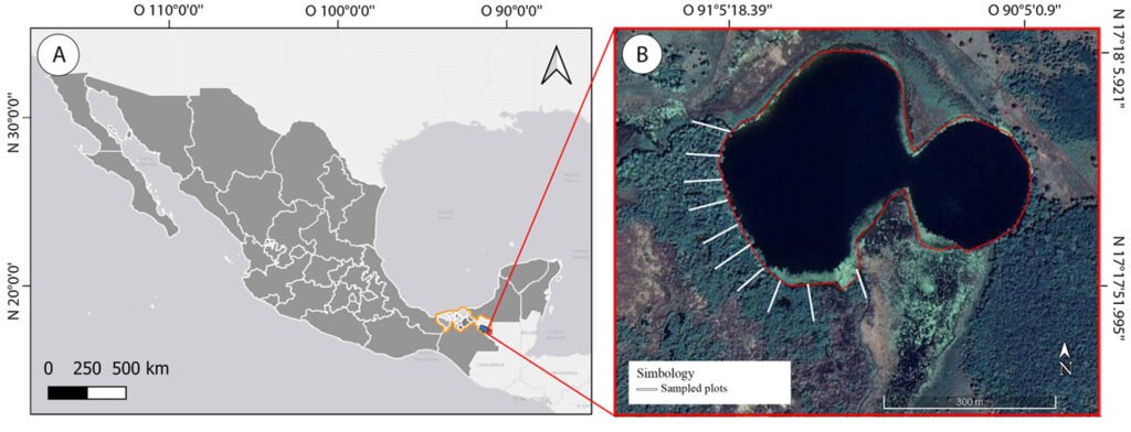
Figure 1. Location of the study area. A) Mexico, highlighting the state of Tabasco (orange) and the municipality of Tenosique (blue). B) El Cacahuate Lagoon (red outline) showing sampling transects (white lines) established in the mangrove vegetation.
The identification of the species was carried out with the support of taxonomic keys and specialized literature for the families Bromeliaceae, Cactaceae, and Orchidaceae (Alderete-Chávez & Capello-García, 1988; Ames & Correll, 1985; Beutelspacher, 2011; Campos-Díaz et al., 2020; Conap, 2010; Davidse et al., 1994; Espejo-Serna et al., 2004; Hágsater et al., 2005; Hietz & Hietz-Seifert, 1994; Martínez-Meléndez et al., 2011; Mondragón-Chaparro et al., 2011; Noguera-Savelli & Cetzal-Ix, 2014), as well as Aspleniaceae, Polypodiaceae, and Pteridaceae (Mickel & Smith, 2004). For species identification, original descriptions were reviewed in the Biodiversity Heritage Library (BHL, 2022). Additionally, to determine the conservation status of the recorded epiphyte species in the study area, we consulted the official Mexican environmental protection and species legislation NOM-059-Semarnat-2010 (Semarnat, 2010) and the Red List of Threatened Species by the International Union for Conservation of Nature (IUCN, 2021).
To determine similarities between the epiphyte species composition of the inland mangrove of El Cacahuate (IM-Cacahuate) and other epiphyte communities, available epiphyte floristic lists from various vegetation types were compiled within a 220 km radius starting from the study area, including sites in Mexico and Guatemala (Fig. 2). Radius length corresponds to the straight-lined distance between El Cacahuate Lagoon and the nearest coastal mangroves of Tabasco, Mexico. It is important to note that most of the studies reviewed were conducted with objectives and sampling efforts not specific to epiphytes, so only the epiphyte species reported were considered (excluding hemiepiphytes).
For the Mexican portion, the compiled lists correspond to coastal mangroves (CM-Paraíso: including localities of Cárdenas, Centla, Comalcalco, Paraíso, Tabasco; Díaz-Jiménez, 2007. CM-Centla: Centla, Tabasco; Jiménez-López et al., 2017, 2018. CM-Nohan: UMA Nohan, Cd. del Carmen, Campeche; Noguera-Savelli et al., 2021); high evergreen tropical forest (HETF-Tenosique: Tenosique, Tabasco, Hernández-Sastré et al., 2014); medium evergreen tropical forest (METF-Macuspana: Macuspana, Tabasco; López-Gómez, 2014; METF-Tenosique: Tenosique, Tabasco; Morales-Damián, 2012); medium subevergreen tropical forest (MSTF-Catazaja: Catazajá, Chiapas; Gutiérrez-Báez, 2004); and tropical dry forest (TDF-Tenosique: Tenosique, Tabasco; Morales-Damián, 2012). Additionally, the riparian flora list of the San Pedro Mártir River was included, which comprises epiphyte records in high, medium, and low evergreen tropical forests with the presence of R. mangle individuals in the riparian vegetation (TF&IM-San Pedro Mártir, Aburto-Oropeza et al., 2021). There are floristic lists that report the presence of epiphyte species for the Calakmul Biosphere Reserve, Campeche, (Conanp, 2023b; Martínez et al., 2001), which were not integrated into the database because this site belongs to the biotic province Yucatán Peninsula (Conanp, 2023b; García-Gil et al., 2002), which reports greater floristic affinity with the districts within the Yucatán Peninsula, Guatemala, and Belize (Duno-de Stefano et al., 2012) and the states of Chiapas, Oaxaca, and Veracruz (Ibarra-Manríquez et al., 2002; Morrone, 2019).
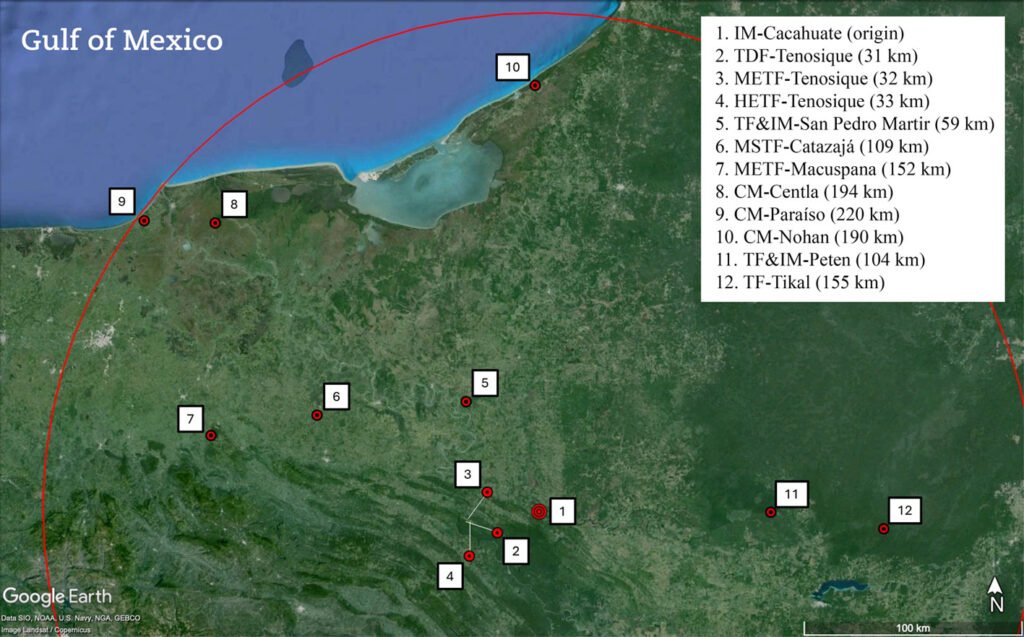
Figure 2. Location of El Cacahuate inland mangrove, the tropical forests, and coastal mangroves within a 220 km radius that include epiphytic floristic lists. The straight-line distance from each site to El Cacahuate is indicated in parentheses. Site acronyms are defined in the Materials and methods section.
In Guatemalan territory, only 2 floristic lists within the established distance for the analysis were obtained: one from a disturbed high evergreen tropical forest (TF-Tikal, Hellmuth & D’Angelo-Jerez, 2022), and the second from a high evergreen tropical forest combined with R. mangle from the El Petén area (TF&IM-Peten, Conap, 2010). Appendix presents the list of the recorded species in the present study and the species compiled from the reviewed studies. The classification of the types of vegetation is based on the proposal of Conabio (2013, 2019) for Chiapas and Tabasco, Mexico, and by Melgar (2003) and Conap (2010) for Tikal and El Petén, Guatemala.
A presence-absence data base was constructed, based on the epiphyte species recorded in our study area and the epiphyte species documented from the surrounding sites obtained of literature. The nomenclature was updated and standardized using the electronic database Tropicos (Tropicos, 2023). Subsequently, the similarity between epiphyte communities of the different vegetation types and locations was explored using the data matrix in a hierarchical clustering analysis (UPGMA) based on the Jaccard similarity index (JSI). This index was selected as it uses species presence-absence data, which was the type of data obtained from the reviewed studies. The measure of similarity ranges from 0% (not similar) to 100% (the most similar). Finally, a beta diversity analysis was performed using Cody’s index (Ci) to assess species turnover between communities. If a high index is obtained, it means that the sites are very different, while a low index means that they share most of their species. Both analyses were conducted using the program Past 4.12b (Hammer et al., 2001).
Results
A total of 6 families, 18 genera, and 27 species of epiphytes were recorded (Table 1)in El Cacahuate mangrove, with Orchidaceae and Bromeliaceae being the families with the highest number of species (11 and 10, respectively), followed by Cactaceae and Polypodiaceae (2 species each) and Aspleniaceae and Pteridaceae (1 species each; Fig. 3). The genera with the most species were Tillandsia (Bromeliaceae) with 8 species, and Epidendrum (Orchidaceae) with 3. Among the epiphyte species recorded in El Cacahuate, Asplenium serratum L. is listed as a threatened species under Mexican legislation (Semarnat, 2010), while Tillandsia fasciculata Sw. and Selenicereus grandiflorus (L.) Briton & Rose are cited on the Red List of Threatened Species by IUCN (2021) as species of least concern.
Table 1
List of epiphyte species associated with the mangrove of El Cacahuate Lagoon, Tenosique, Tabasco, Mexico. *New records for the Wanha’ Biosphere Reserve.
| Family | Species |
| Aspleniaceae | Asplenium serratum L.* |
| Bromeliaceae | Aechmea bracteata (Sw.) Griseb. |
| Catopsis morreniana Mez | |
| Tillandsia balbisiana Schult. & Schult.f. | |
| T. brachycaulos Schltdl. | |
| T. bulbosa Hook. | |
| T. dasyliriifolia Baker* | |
| T. fasciculata Sw. | |
| T. juncea (Ruiz & Pav.) Poir. | |
| T. schiedeana Steud. | |
| T. streptophylla Scheidw. Ex E.Morren | |
| Cactaceae | Deamia testudo (Karw. Ex Zucc.) Britton & Rose |
| Selenicereus grandiflorus (L.) Briton & Rose | |
| Orchidaceae | Catasetum integerrimum Hook. |
| Cohniella ascendens (Lindl.) Christenson | |
| Encyclia bractescens (Lindl.) Hoehne | |
| Epidendrum cardiophorum Schltr. | |
| E. diffusum Sw.* | |
| E. nocturnum Jacq. | |
| Myrmecophila tibicinis (Bateman) Rolfe | |
| Nidema boothi (Lindl.) Schltr.* | |
| Notylia barkerii Lindl.* | |
| Oncidium sphacelatum Lindl. | |
| Specklinia grobyi (Bateman ex Lindl.) F.Barros | |
| Polypodiaceae | Microgramma nítida (J. Sm.) A.R. Sm.* |
| Polypodium polypodioides (L.) Watt* | |
| Pteridaceae | Vittaria lineata (L.) Sm. |
Similarities between epiphyte communities. The present study and the review of published studies within the selected surrounding area allowed for the compilation of a total of 119 epiphyte species from sites with coastal mangrove, inland mangrove, tropical forests, and disturbed forests (Appendix). The sites with the highest number of epiphyte species were the high evergreen tropical forest of Tenosique (HETF-Teno, 53 species), the riparian vegetation of the San Pedro River (TF&IM-SPMR, 52 species), the medium evergreen tropical forest of Macuspana (METF-Macus, 45 species), the inland mangrove of El Cacahuate Lagoon (IM-Cac, 27 species), and the coastal mangrove of Centla (CM-Centla, 25 species). In the remaining sites, the number of epiphyte species ranged from 4 to 16, with 14 species recorded in the coastal mangroves of Nohan and Paraíso (CM-Nohan, CM-Paraíso; Appendix).
The clustering analysis (Fig. 4) clearly separated 4 groups (at a similarity level of 0.14). Two groups consisted of a single location: the first being the disturbed evergreen tropical forest of Tikal (TF-Tikal) and the second, the medium subevergreen tropical forest of Catazaja, Chiapas (MSTF-Catazaja). The other 2 groups contained several locations. The first group was made up of different forest types in Tabasco (HETF-Tenosique, METF-Macuspana, TDF-Tenosique, METF-Tenosique), while the second group included sites with coastal mangroves (CM-Nohan, CM-Paraíso, CM-Centla) and tropical forest and inland mangrove vegetation (TF&IM-San Pedro Mártir, TF&IM-Peten, IM-Cacahuate). In this latter group, the inland mangrove of El Cacahuate showed greater similarity in the epiphyte species with the coastal mangroves of Centla (JSI = 0.45, 16 shared species) and Paraíso (JSI = 0.38, 11 shared species), despite being 194 and 220 km away from El Cacahuate, respectively. The tropical forest and mangrove vegetation of the San Pedro River shared a greater number of species (19) with the El Cacahuate mangrove, but the similarity was slightly lower (JSI = 0.23), although the distance between these sites is lower, 59 km. The next ecosystem is the forest with inland mangrove of El Petén, sharing 8 species with El Cacahuate and showing a lower similarity than the previous groups (JSI = 0.18). At last, the coastal mangrove of Nohan, Campeche shared 7 species with El Cacahuate, with the lower similarity inner this group (JSI = 0.15).
Among all groups, the lowest similarity of the epiphyte community of El Cacahuate was with the medium subevergreen tropical forest of Catazaja (JSI = 0.05) and the disturbed evergreen tropical forest of Tikal (JSI = 0.03), with 2 and 1 species in common, respectively; both located over 100 km from El Cacahuate Lagoon. Among sites with mangrove vegetation, beta diversity analysis (Table 2) shows that the inland mangrove of El Cacahuate presents low species turnover with the coastal mangroves (Centla and Paraíso; Ci= 10 and 9.5, respectively). In contrast, species turnover is higher with the riparian forest and mangrove vegetation of the San Pedro Mártir River (Ci= 19).
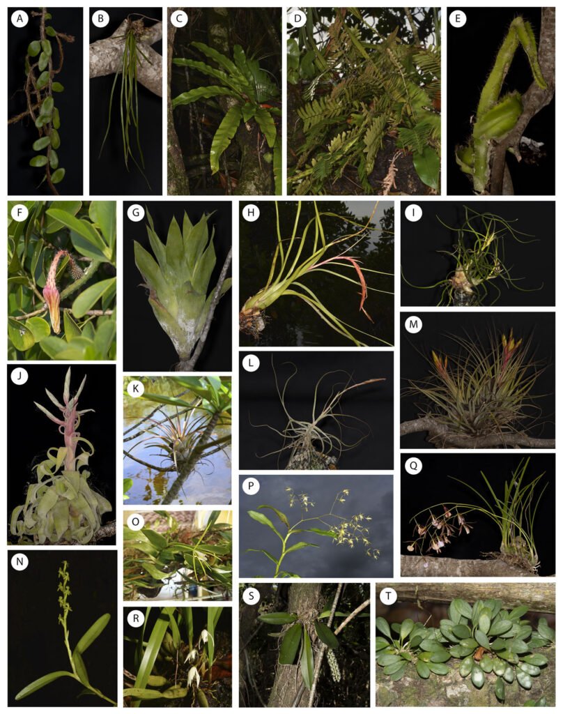
Figure 3. Representative epiphyte species recorded in the inland mangrove of El Cacahuate Lagoon, Tenosique, Tabasco, Mexico. A) Microgramma nitida, B) Vittaria lineata, C) Asplenium serratum, D) Polypodium polypodioides, E) Deamia testudo, F) Selenicereus grandiflorus, G) Catopsis morreniana, H) Tillandsia balbisiana, I) T. bulbosa, J) T. streptophylla, K) T. dasyliriifolia, L) T. schiedeana, M) T. fasciculata, N) Epidendrum cardiophorum, O) E. nocturnum, P) E. diffusum, Q) Encyclia bractescens, R) Nidema boothi, S) Notylia barkerii, and T) Specklinia grobyi. Photographs by Jesús Rodríguez and Neil Morales.
Discussion
As far as we know, our study is the first to be conducted on epiphytic species of inland mangroves in El Cacahuate Lagoon. The epiphyte community of El Cacahuate Lagoon, with 27 records species, is among the richest ever reported in a mangrove ecosystem. Previous studies have reported the presence of fewer species in coastal mangroves (De Sousa & Colpo, 2017; Díaz-Jiménez, 2007; Jiménez-López et al., 2017, 2018; Menéndez-Liguori, 1976; Noguera-Savelli et al., 2021; Rohani et al., 2020). However, it is true that many of these studies did not involve extensive sampling, or they were not specifically focused on epiphyte species. Jiménez-López et al. (2017, 2018), in the mangrove of El Cometa Lagoon, Centla, Tabasco, were specifically focused on epiphytes, recording 25 species. In contrast, the tropical forest sites of Tenosique and Macuspana (Hernández-Sastré et al., 2014; López-Gómez, 2014; Morales-Damián, 2012), and the riparian forest and mangrove of San Pedro Mártir, Tabasco (Aburto-Oropeza et al., 2021), have a higher reported number of epiphyte species than the mangrove of El Cacahuate. However, these differences in the number of species reported are because the forests of Tenosique, Macuspana, and the San Pedro Mártir River were collected in larger areas of vegetation, a greater number of phorophyte species were sampled, and different sampling methods were used. For example: A) in the forests of Tenosique (Morales-Damián, 2012; Hernández-Sastré et al., 2014) sampled 25 × 25 m plots, recording the epiphytes associated with 9 species of phorophytes; B) in the Macuspana forest (López-Gómez, 2014), a representative sampling method of 1 ha was used, sampling epiphytes in 8 plots of 20 × 20 m (400 m²), considering both trees and shrubs present; and finally C) on the San Pedro Mártir River (Aburto-Oropeza et al., 2021), targeted sampling was carried out between 2014 and 2015 with sporadic collections until 2019, covering more than 25 linear km of river and sampling more than 30 species of phorophytes (Burelo-Ramos pers. com.). This shows that floristic lists targeting forests tend to have higher reports of epiphytes than mangrove ecosystems.
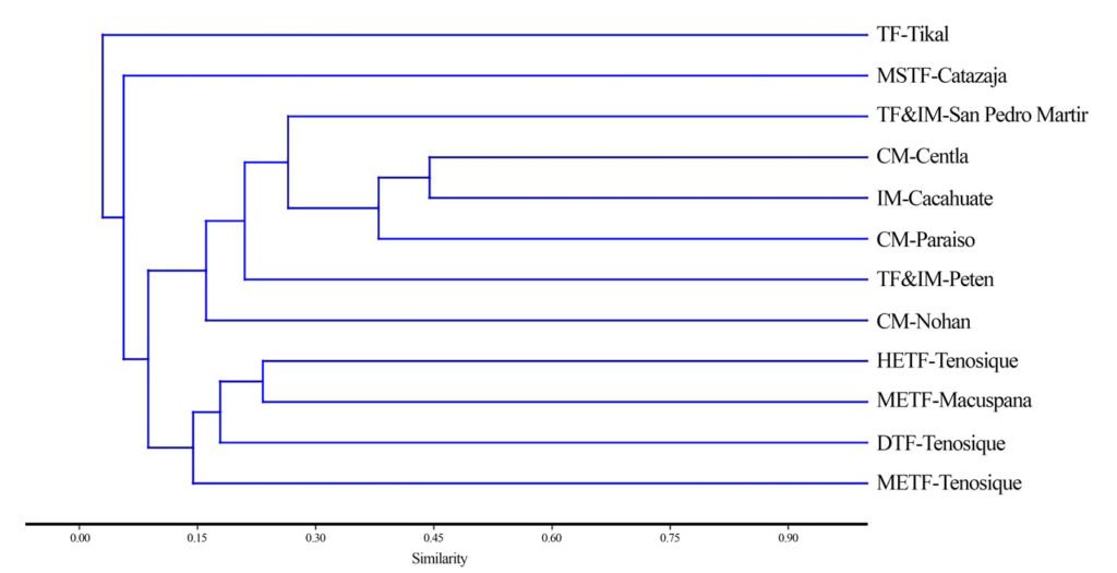
Figure 4. Dendrogram showing the similarity of epiphyte communities among the El Cacahuate Lagoon mangrove, coastal mangroves, and adjacent forest vegetation sites. Site acronyms are defined in the Materials and Methods section.
Table 2
Beta-diversity of epiphytes between the inland mangrove of El Cacahuate Lagoon and epiphyte floristic lists of surrounding tropical forest and coastal mangroves. Values above the diagonal represent Cody’s index for each pairwise comparison. Values below the diagonal indicate the number of shared species between sites. The top row displays the total species richness for each location. The first column lists the number of species unique to each site. Site acronyms are defined in the Materials and methods section.
| Total | 27 | 11 | 9 | 47 | 51 | 4 | 43 | 25 | 14 | 14 | 16 | 5 | |
| Unique | sites | IM-Cacahuate | TDF-Tenosique | METF-Tenosique | HETF-Tenosique | TF&IM-San Pedro | MSTF-Catazaja | METF-Macuspana | CM-Centla | CM-Paraíso | CM-Nohan | TF&IM-Peten | TF-Tikal |
| 0 | IM-Cacahuate | 12 | 15 | 23 | 19 | 13.5 | 29 | 10 | 9.5 | 13.5 | 13.5 | 15 | |
| 0 | TDF-Tenosique | 7 | 8 | 19 | 25 | 6.5 | 20 | 15 | 10.5 | 11.5 | 13.5 | 8 | |
| 0 | METF-Tenosique | 3 | 2 | 19 | 27 | 6.5 | 20 | 16 | 9.5 | 10.5 | 12.5 | 7 | |
| 11 | HETF-Tenosique | 14 | 10 | 9 | 32 | 24.5 | 28 | 29 | 24.5 | 26.5 | 28.5 | 24 | |
| 14 | TF&IM-SPMR | 20 | 6 | 3 | 17 | 24.5 | 32 | 23 | 21.5 | 26.5 | 24.5 | 25 | |
| 1 | MSTF-Catazaja | 2 | 1 | 0 | 1 | 3 | 21.5 | 11.5 | 8 | 7 | 10 | 4.5 | |
| 15 | METF-Macuspana | 5 | 6 | 6 | 17 | 15 | 2 | 28 | 26.5 | 26.5 | 29.5 | 24 | |
| 3 | CM-Cent | 16 | 3 | 1 | 7 | 15 | 3 | 6 | 8.5 | 11.5 | 13.5 | 14 | |
| 1 | CM-Para | 11 | 2 | 2 | 6 | 11 | 1 | 2 | 11 | 10 | 9 | 8.5 | |
| 5 | CM-Nohan | 7 | 1 | 1 | 4 | 6 | 2 | 2 | 7 | 4 | 13 | 9.5 | |
| 4 | TF&IM-Peten | 8 | 0 | 0 | 3 | 9 | 0 | 0 | 7 | 6 | 2 | 8.5 | |
| 1 | TF-Tikal | 1 | 0 | 0 | 2 | 3 | 0 | 0 | 1 | 1 | 0 | 2 |
The low richness of epiphytes in coastal mangroves has been associated with the adverse environmental conditions present, such as high temperatures, low precipitation, and excess salinity (Benzing, 1990; Carmona-Díaz et al., 2014; García-Luna et al., 2024; Gómez & Winker, 1991; Zimmerman & Olmsted, 1992; Zotz & Reuter, 2009). Mangrove trees eliminate excess salt through their leaves (Mikolaev et al., 2016; Zotz & Reuter, 2009), so large amounts of salt could be accumulating in some epiphytes (e.g., orchids and bromeliads) due to leaf litter and rainwater falling from the canopy, which is captured in the roots and the rosette leaves of these plants. Salt decreases the osmotic potential of epiphyte cells, reducing their survival by promoting tissue necrosis and leaf loss, especially for species that do not have adaptations to survive under extreme water stress conditions, v.gr., xerophytic habits (Benzing, 2000; Du & Hesp, 2020; Zotz & Reuter, 2009). However, Gómez and Winkler (1991) have pointed out a contrary position suggesting that the high precipitation in some coastal areas may dilute the high salinity that falls from the mangrove’s canopy, allowing for the existence of non-xerophytic epiphytes. Nevertheless, the low presence of epiphyte species in mangrove ecosystems suggests that the physiological limitations in many of these plants may be significant (Cach-Pérez et al., 2018). Considering the distribution of mangroves worldwide, more floristic studies are needed in this ecosystem to identify patterns in other epiphytes species numbers, physiological traits, and functional groups.
The mangrove of El Cacahuate Lagoon presents a less stressful environment compared to coastal mangroves, as it is in a freshwater body with high precipitation (annual average of 2,300 mm) and warm temperatures (annual average of 26 °C) (Aceves-Navarro & Rivera-Hernández, 2019). In coastal mangroves, which are characterized as saline ecosystems (Feller et al., 2010), R. mangle eliminates the excess of salt absorbed by its roots through lenticels on its leaves (Bento et al., 2024). However, although El Cacahuate Lagoon is a freshwater aquatic system (0.4 psu) compared to nearby coastal sites (22 psu), calcium carbonate from mountain runoff has been reported in the area (Aburto-Oropeza et al., 2021; Conanp, 2023a) and the sap salinity of the plants is like that of trees in coastal areas (J. López-Portillo pers. com.). This suggests that the R. mangle trees in El Cacahuate Lagoon still exude salt through the leaves. However, atmospheric humidity and high precipitation could dilute the concentration of salts reaching the epiphytes (J. López-Portillo pers. com.). These conditions seem to favor the presence of orchid, bromeliad, and fern species recorded at this site; it also suggests that the species shared between the inland mangrove and coastal mangroves have adapted to both environmental conditions. Specific ecophysiological studies of the shared and not shared epiphyte species between this inland mangrove and the coastal mangroves will provide a better understanding of the characteristics that limit and promote the distribution of epiphytes in these ecosystems.
Similarities between epiphyte communities. Given the proximity of the Tenosique mountain (ca. 2-32 km), we expected that the species composition of the study area showed greater similarity in epiphyte composition with the surrounding forests (HETF, METF, DTF). It has been recorded that the structure, anatomy, and seed dispersal mechanisms of many epiphytes permit frequent colonization and recolonization processes between nearby tropical sites (Chilpa-Galván et al., 2018; Toledo-Aceves et al., 2012). Nevertheless, we found the highest similarity of El Cacahuate mangrove’s epiphyte species with the epiphyte communities of the coastal mangroves of Centla and Paraíso, located 194-200 km away. These facts suggest 2 possible hypotheses which can help to explain these similarities: the first suggests that when the sea encroached 120,000 years ago, not only R. mangle individuals and other terrestrial coastal species established along the banks of the San Pedro River and El Cacahuate Lagoon, but this process was accompanied by the coastal-affinity epiphytes recorded in the study area; the second one points to contemporary dispersal processes as the reason for the presence of these epiphytes with a coastal distribution. It has been documented that after ca. 30 years, 30% of the original epiphyte species recorded in mangrove trees in the natural part of a canal, colonized juvenile mangroves planted for reforestation in the artificial part of the canal (Kupec, 2018). This suggests that the epiphyte species with coastal affinity may have arrived at the inland mangrove of El Cacahuate Lagoon by seed step-dispersal and colonization events throughout the mangrove established along the San Pedro River, or by long-distance dispersal events of minute seed from the coastal mangroves (Schurr et al., 2009). The other epiphyte species with extensive tropical forest distribution surely have arrived by both dispersal ways.
These 2 processes do not exclude each other, and their success can be highly dependent on the number of viables seeds and habitat availability (Rodríguez-Romero et al., 2011). However, successful establishment also depends on the morphological and anatomical characteristics of the seeds (Arditti & Ghani, 2000; Chilpa-Galván et al., 2018). For instance, some ferns families (e.g., Aspleniaceae, Polypodiaceae, and Pteridaceae) produce many very small spores that are easily dispersed by wind over long distances (Martínez-Salas & Ramos, 2014; Perrie et al., 2010; Shepherd et al., 2009). Similarly, orchid fruits (Orchidaceae) produce millions of tiny seeds, often just a few microns in size and weighing no more than 22 mcg (Arditti & Ghani, 2000; Menchaca-García & Moreno-Martínez, 2011), which are also adapted for long-distance wind dispersal. Many bromeliad species (Bromeliaceae, subfamily Tillandsoideae) have plumose seed appendages that facilitate their movement through the air and their attachment to rough bark surfaces (Einzmann & Zotz, 2017; Mondragón-Chaparro et al., 2011). Meanwhile, some species such as A. bracteata, which produce berry-like fruits, and cacti such as S. grandiflorus and D. testudo, which have pulpy fruits, are dispersed by birds. This suggests that short- or long-distance seed dispersal has contributed to structuring the epiphyte community in the inland mangrove of El Cacahuate Lagoon. Future genetic studies will reveal how closely related the populations of shared epiphyte species are between the inland mangroves of El Cacahuate Lagoon and the coastal mangroves of Tabasco, particularly for those species with a wide distribution range.
Our study clearly shows that the epiphyte community in the inland mangroves of El Cacahuate Lagoon is species-rich. The humid environmental conditions present apparently reduce the salinity concentration exuded by the mangrove trees, allowing the great epiphyte species richness recorded. Also, we have demonstrated that this epiphyte community has a high similarity in composition to the epiphyte communities of the coastal mangroves of Tabasco, suggesting a close genetic relationship between these populations. Future genetic studies will help elucidate the dispersal routes followed by the epiphytes to colonize this mangrove. These and other biological characteristics make this inland mangrove ecosystem one of great biodiversity and conservation value.
Acknowledgments
Special thanks to the UJAT herbarium for access to its facilities and the support provided during the cabinet phase. We are grateful to M. Ferrer, J. Rodríguez, and E. López for their help with the fieldwork. Special thanks to W. Miss and his family for their hospitality and for facilitating access to the study site. Thanks to S. Morales, C. Rodríguez, and I. Morales for providing transportation to the study site. We extend our gratitude to F. Jiménez H. and R. Adams for reviewing early drafts of this manuscript. This study is part of the requirements for obtaining a master’s degree for NEM. The work was supported by the Universidad Juárez Autónoma de Tabasco through the project “Biodiversity and conservation of the inland mangroves of the San Pedro Mártir River as elements for sustainable development in Balancán and Tenosique, Tabasco, Mexico” (No. 20220327), and the Centro para la Biodiversidad Marina y la Conservación, A.C. and Mares Mexicanos. The Consejo Nacional de Humanidades, Ciencia y Tecnología (Conahcyt) granted a scholarship to the first author for his master’s program.
Appendix. Checklist of vascular epiphytes recorded in the inland mangrove of El Cacahuate Lagoon, and compiled data from the floristic studies completed in a radius of 220 km from El Cacahuate Lagoon. Acronyms: IM-Cacahuate, inland mangrove of El Cacahuate, Tenosique, Tabasco; CM-Paraíso, coastal mangrove of Cárdenas, Centla, Comalcalco, Paraíso, Tabasco (Díaz-Jiménez, 2007); CM-Centla, coastal mangrove of Centla, Tabasco (Jiménez-López et al., 2017, 2018); CM-Nohan, coastal mangrove of the UMA Nohan, Cd. del Carmen, Campeche (Noguera-Savelli et al., 2021); HETF-Tenosique, high evergreen tropical forest of Tenosique, Tabasco (Hernández-Sastré et al., 2014); METF-Tenosique, medium evergreen tropical forest of Tenosique, Tabasco (Morales-Damián, 2012); METF-Macuspana: Macuspana, Tabasco; López-Gómez 2014); MSTF-Catazaja: medium subevergreen tropical forest of Catazajá, Chiapas (Gutiérrez-Báez, 2004); TDF-Tenosique: tropical dry forest of Tenosique, Tabasco (Morales-Damián, 2012); TF&IM-San Pedro Mártir: tropical forests with the presence of R. mangle individuals in the riparian vegetation of the San Pedro Mártir River (Aburto-Oropeza et al., 2021); TF-Tikal: disturbed high evergreen tropical forest (Hellmuth and D’Angelo-Jerez, 2022); TF&IM-Peten: high evergreen tropical forest combined with R. mangle from the El Petén area (Conap, 2010).
| Families | Species /sites | IM-Cacahuate | TDF-Tenosique | METF-Tenosique | HETF-Tenosique | TF&IM-San Pedro Mártir | MSTF-Catazaja | METF-Macuspana | CM-Centla | CM-Paraíso | CM-Nohan | TF&IM-Petén | TF-Tikal |
| Aspleniaceae | Asplenium auritum Sw. | x | |||||||||||
| Asplenium serratum L. | x | x | |||||||||||
| Bromeliaceae | Aechmea bracteata (Sw.) Griseb. | x | x | x | x | x | x | ||||||
| Aechmea mexicana Baker | x | ||||||||||||
| Aechmea tillandsoides (Mart. ex Schult. & Schult.f.) Baker | x | ||||||||||||
| Billbergia viridiflora H.Wendl. | x | ||||||||||||
| Catopsis morreniana Mez | x | x | |||||||||||
| Catopsis nutans (Sw.) Griseb. | x | ||||||||||||
| Tillandsia anceps G. Lodd. | x | ||||||||||||
| Tillandsia balbisiana Schult. & Schult.f. | x | x | x | x | x | x | |||||||
| Tillandsia brachycaulos Schltdl. | x | x | x | x | x | ||||||||
| Tillandsia bulbosa Hook. | x | x | x | x | x | ||||||||
| Tillandsia chlorophylla L. B. Smith | x | ||||||||||||
| Tillandsia dasyliriifolia Baker | x | x | x | x | |||||||||
| Tillandsia fasciculata Sw. | x | x | x | x | |||||||||
| Tillandsia festucoides Brongn. Ex Mez | x | x | |||||||||||
| Tillandsia filifolia Schldtl. & Cham. | x | x | |||||||||||
| Tillandsia ionantha Planch | x | ||||||||||||
| Tillandsia juncea (Ruiz & Pav.) Poir. | x | x | x | x | |||||||||
| Tillandsia recurvata (L.) L. | x | ||||||||||||
| Tillandsia polystachia (L.) L. | x | ||||||||||||
| Tillandsia pseudobaileyi C.S. Gardner | x | ||||||||||||
| Tillandsia pruinosa Sw. | x | ||||||||||||
| Tillandsia schiedeana Steud. | x | x | x | x | x | ||||||||
| Tillandsia streptophylla Scheidw. Ex E.Morren | x | x | x | x | x | x | |||||||
| Tillandsia usneoides (L.) L. | x | x | x | x | x | ||||||||
| Tillandsia valenzuelana A. Rich | x | ||||||||||||
| Cactaceae | Deamia testudo (Karw. Ex Zucc.) Britton & Rose | x | x | x | x | x | x | ||||||
| Pseudorhipsalis ramulosa (Salm-Dyck) Barthlott | x | ||||||||||||
| Epiphyllum crenatum (Lindl.) G.Don | x | ||||||||||||
| Epiphyllum hookeri Haw. | x | x | |||||||||||
| Epiphyllum phyllanthus (L.) Haw. | x | x | x | ||||||||||
| Rhipsalis baccifera (J.S. Muell.) Stearn | x | x | |||||||||||
| Selenicereus donkelaarii (Salm-Dick) Britton & Rose | x | ||||||||||||
| Selenicereus grandiflorus (L.) Briton & Rose | x | x | x | x | |||||||||
| Selenicereus undatus (Haw.) D.R. Hunt | x | ||||||||||||
| Gesneriaceae | Columnea schiedeana Schltdl. | x | |||||||||||
| Orchidaceae | Acianthera hondurensis (Ames) Pridgeon & M. W. Chase | x | x | ||||||||||
| Brassavola nodosa (L.) Lindl. | x | x | |||||||||||
| Brassia caudata (L.) Lindl. | x | x | |||||||||||
| Brassia maculata R. Br. | x | x | |||||||||||
| Camaridium pulchrum Schltr. | x | x | |||||||||||
| Campylocentrum micranthum (Lindl.) Maury | x | x | |||||||||||
| Catasetum integerrimum Hook. | x | x | x | x | x | x | x | x | |||||
| Chysis bractescens Lindl. | x | x | x | ||||||||||
| Coelia triptera (Sm.) G. Don ex Steud. | x | x | x | ||||||||||
| Cohniella ascendens (Lindl.) Christenson | x | x | x | x | x | x | x | ||||||
| Cohniella cosymbephorum (C. Morren) R. Jiménez & Carnevali | x | ||||||||||||
| Cohniella lindenii (Brongn.) M.W.Chase & N.H.Williams | x | x | |||||||||||
| Cohniella luridum (Lindl.) M.W. Chase & N.H. Williams | x | x | x | ||||||||||
| Cohniella Yucatánensis Cetzal & Carnevali | x | ||||||||||||
| Coryanthes picturata Rchb.f. | x | x | |||||||||||
| Cycnoches ventricosum Bateman | x | ||||||||||||
| Dichaea muricatoides Hamer & Garay | x | ||||||||||||
| Dichaea panamensis Lindl. | x | ||||||||||||
| Encyclia alata (Bateman) Schltr. | x | x | x | ||||||||||
| Encyclia bractescens (Lindl.) Hoehne | x | x | x | x | |||||||||
| Encyclia guatemalensis (Klotzsh) Dressler & G.E. Pollard | x | ||||||||||||
| Epidendrum anceps Jacq. | x | ||||||||||||
| Epidendrum cardiophorum Schltr. | x | x | x | ||||||||||
| Epidendrum difforme Jacq. | x | x | |||||||||||
| Epidendrum diffusum Sw. | x | x | x | ||||||||||
| Epidendrum flexuosum G. Mey. | x | x | |||||||||||
| Epidendrum nocturnum Jacq. | x | x | x | x | x | ||||||||
| Epidendrum stamfordianum Bateman | x | x | x | ||||||||||
| Gongora leucochila Lem. | x | x | |||||||||||
| Gongora unicolor Rolfe | x | ||||||||||||
| Isochilus carnosiflorus Lindl. | x | x | x | ||||||||||
| Lophiaris lindenii (Brongn.) Braem | x | x | |||||||||||
| Lophiaris oerstedii (Rchb. f.) R. Jiménez Carnevali & Dressler | x | x | x | x | x | ||||||||
| Lophiaris teaboana R. Jiménez, Carnevali & Tapia Muñoz | x | ||||||||||||
| Lycaste aromatica (Graham) Lindl. | x | ||||||||||||
| Maxillaria aciantha Rchb. f. | x | ||||||||||||
| Maxillaria crassifolia (Lindl.) Rchb. f. | x | x | x | x | |||||||||
| Maxillaria elatior (Rchb. f.) Rchb. f. | x | x | |||||||||||
| Maxillaria hedwigiae Hamer & Dodson | x | ||||||||||||
| Maxillaria tenuifolia Lindl. | x | x | |||||||||||
| Maxillaria uncata Lind. | x | ||||||||||||
| Maxillaria variabilis Bateman ex Lindl. | x | x | |||||||||||
| Myrmecophila christinae var. christinae Carnevali & Gómez-Juárez | x | ||||||||||||
| Myrmecophila tibicinis (Bateman) Rolfe | x | x | x | x | x | x | |||||||
| Nemaconia striata (Lindl.) Van den Berg, Salazar & Soto Arenas | x | x | |||||||||||
| Nidema boothi (Lindl.) Schltr. | x | x | x | x | x | x | |||||||
| Notylia barkeri Lindl. | x | x | x | x | x | x | |||||||
| Notylia orbicularis A.Rich. | x | ||||||||||||
| Oncidium sphacelatum Lindl. | x | x | x | x | x | ||||||||
| Ornithocephalus inflexus Lindl. | x | x | |||||||||||
| Platystele minimiflora (Schltr.) Garay | x | ||||||||||||
| Platythelys querceticola (Lindl.) Garay | x | ||||||||||||
| Platystele stenostachya (Rchb.f.) Garay | x | ||||||||||||
| Polystachya caracasana Rchb.f. | x | ||||||||||||
| Prosthechea cochleata (L.) W.E.Higgins | x | x | x | ||||||||||
| Prosthechea boothiana (Lindl.) W.E.Higgins | x | ||||||||||||
| Prosthechea livida (Lindl.) W.E.Higgins | x | ||||||||||||
| Prosthechea pygmaea (Hook.) W. E. Higgins | x | ||||||||||||
| Prosthechea radiata (Lindl.) W. E. Higgins | x | ||||||||||||
| Restrepiella ophiocephala (Lindl.) Garay & Dunst. | x | ||||||||||||
| Sarcinula brighamii (S. Watson) Luer | x | ||||||||||||
| Scaphyglottis confusa (Schltr.) Ames & Correll | x | x | |||||||||||
| Specklinia grobyi (Bateman ex Lindl.) F.Barros | x | x | |||||||||||
| Specklinia picta (Lindl.) Pridgeon & M.W. Chase | x | ||||||||||||
| Specklinia pisinna (Luer) Solano y Soto Arenas | x | ||||||||||||
| Stelis gracilis Ames | x | ||||||||||||
| Tribulago tribuloides (Sw.) Luer | x | ||||||||||||
| Trichosalpinx ciliaris (Lindl.) Luer | x | ||||||||||||
| Trigonidium egertonianum Bateman ex Lindl. | x | x | x | x | |||||||||
| Piperaceae | Peperomia angustata Kunth | x | |||||||||||
| Peperomia cobana C.DC. | x | ||||||||||||
| Peperomia glutinosa Millsp. | x | ||||||||||||
| Peperomia obtusifolia (L.) A.Dietr. | x | ||||||||||||
| Peperomia quadrifolia (L.) Kunth | x | ||||||||||||
| Peperomia rotundifolia (L.) Kunth | x | ||||||||||||
| Polypodiaceae | Campyloneurum angustifolium (Sw.) Fée | x | |||||||||||
| Neurodium lanceolatum (L.) Fée | x | ||||||||||||
| Microgramma nitida (J. Sm.) A.R. Sm. | x | x | |||||||||||
| Phlebodium decumanum (Willd.) J. Sm. | x | ||||||||||||
| Polypodium polypodioides (L.) Watt | x | x | x | ||||||||||
| Pteridaceae | Antrophyum ensiforme Hook. | x | |||||||||||
| Vittaria lineata (L.) Sm. | x | x | x |
References
Aburto-Oropeza, O., Burelo-Ramos, C. M., Ezcurra, E., Ezcurra, P., Henriquez, C. L., Vanderplank, S. et al. (2021). Relict inland mangrove ecosystem reveals Last Interglacial sea levels. Proceedings of the National Academy of Sciences, 118, 1–8. https://doi.org/10.1073/pnas.2024518118
Aceves-Navarro, L. A., & Rivera-Hernández, B. (2019). Clima. In A. Cruz Angón (Ed.), La biodiversidad del estado de Tabasco. Estudio de estado (pp. 123–132). México, D.F.: Comisión Nacional para el Conocimiento y Uso de la Biodiversidad.
Aksornkoae, S. (1993). Ecology and management of mangroves. Bangkok, Thailand: International Union for Conservation of Nature (IUCN). https://portals.iucn.org/library/sites/library/files/documents/WTL-024.pdf
Alderete-Chávez, A., & Capello-García, S. (1988). Orquídeas de Tabasco. Villahermosa: Instituto Nacional de Investigaciones sobre Recursos Bióticos/ Instituto de Cultura de Tabasco.
Ames, O., & Correll, D. S. (1985). Orchids of Guatemala and Belize. New York: Dover Publications.
Arditti, J., & Ghani, A. K. A. (2000). Numerical and physical properties of orchid seeds and their biological implications. New Phytologist, 145, 367–421. https://doi.org/10.1046/j.1469-8137.2000.00587.x
Bento, J. P. S. P., Victório, C. P., Plaça, L. F., Arruda, R. C. O. (2024). Salt extrusion, a new function of lenticels in red mangrove leaves. Environmental and Experimental Botany, 223, 05798. https://doi.org/10.1016/j.envexpbot.2024.105798
Benzing, D. H. (1990). Vascular epiphytes: general biology and related biota. Cambridge, UK: Cambridge University Press.
Benzing, D. H. (2000). Bromeliaceae: profile of an adaptative radiation. Cambridge, UK: Cambridge University Press.
Beutelspacher, C. R. (2011). Guía de orquídeas de Chiapas. Tuxtla Gutiérrez, Chiapas: Universidad de Ciencias y Artes de Chiapas. Chiapas
BHL (Biodiversity Heritage Library) (2022). Available at: https://www.biodiversitylibrary.org
Cach-Pérez, M. J., Andrade, J. L., Chilpa-Galván, N., Tamayo-Chim, M., Orellana, R., & Reyes-García, C. (2013). Climatic and structural factors influencing epiphytic bromeliad community assemblage along a gradient of water-limited environments in the Yucatán Peninsula, Mexico. Tropical Conservation Science, 6, 283–302. https://doi.org/10.1177/194008291300600209
Campos-Díaz, M. J., Burelo-Ramos, C. M., & Arias, S. (2020). La familia Cactaceae en Tabasco, México. Acta Botanica Mexicana, 127, e1635. https://doi.org/10.21829/abm127.2020.1635
Carmona-Díaz, G., Hernández-Carmona, S., Morales-Mávil, J. E., Hernández-Salazar, L. T., & García-Orduña, F. (2014). Contribución al conocimiento ecológico de la epífita vascular Aechmea bracteata (Bromeliaceae) en el manglar de Sontecomapan, Catemaco, Veracruz, México. Revista Científica Biológico Agropecuario, Tuxpan, 2, 816–821.
Carmona-Higuita, M. J., Mendieta-Leiva, G., Gómez-Díaz, J. A., Villalobos, F., Ramos, F. N., Elias, J. P. C. et al. (2025). Endemism centres of the five richest vascular epiphyte families in the Neotropics. Journal of Biogeography, 52, 80–91. https://doi.org/10.1111/jbi.15016
Ceja-Romero, J., Espejo-Serna, A., López-Ferrari, A. R., García-Cruz, J., Mendoza-Ruiz, A., & Pérez-García, B. (2008). Las plantas epífitas, su diversidad e importancia. Ciencias, 1, 34–41.
Chilpa-Galván, N., Márquez-Guzmán, J., Zotz, G., Echevarría-Machado, I., Andrade, J. L., Espadas-Manrique, C. et al. (2018). Seed traits favouring dispersal and establishment of six epiphytic Tillandsia (Bromeliaceae) species. Seed Science Research, 28, 349–359. https://doi.org/10.1017/S0960258518000247
Conabio (Comisión Nacional para el Conocimiento y Uso de la Biodiversidad) (2013). La biodiversidad en Chiapas: Estudio de Estado. México: Conabio/ Gobierno del Estado de Chiapas.
Conabio (Comisión Nacional para el Conocimiento y Uso de la Biodiversidad) (2019). La biodiversidad en Tabasco. Estudio de Estado. México: Conabio. https://bioteca.biodiversidad.gob.mx/janium/Documentos/14868.pdf
Conap (Consejo Nacional de Áreas Protegidas) (2010). Guía de reconocimiento del género Tillandsiade Guatemala. Guatemala. https://www.caftadr-environment.org/wp-cont
ent/uploads/2016/04/guia-de-Reconocimiento-de-Tillandsia-2.pdf
Conanp (Comisión Nacional de Áreas Naturales Protegidas) (2015). Área de protección de flora y fauna Cañon del Usumacinta. México: Semarnat/ Conanp. https://www.
conanp.gob.mx/que_hacemos/pdf/programas_manejo/2015/Canon_del_Usumacinta.pdf
Conanp (Comisión Nacional de Áreas Naturales Protegidas) (2023a). Estudio previo justificativo para el establecimiento del Área Natural Protegida Reserva de la Biósfera Wanha’.Tabasco, México. https://www.conanp.gob.mx/pdf/separata/EPJ-RB-Wanha.pdf
Conanp (Comisión Nacional de Áreas Naturales Protegidas) (2023b). Estudio previo justificativo para la modificación de la declaratoria del Área Natural Protegida Reserva de la Biosfera Calakmul, Campeche, México. https://www.conanp.gob.mx/pdf/separata/EPJ-Modificacion-RB-Calakmul.pdf
Davidse, G., Sousa-Sánchez, M., & Chater, A. O. (1994). Alismataceae a Cyperaceae. In G. Davidse (Ed.), Flora mesoamericana (pp. 1–543). México D.F.: Universidad Nacional Autónoma de México.
De Sousa, M. M., & Colpo, K. D. (2017). Diversity and distribution of epiphytic bromeliads in a Brazilian subtropical mangrove. Anais da Academia Brasileira de Ciências, 89, 1085–1093. https://doi.org/10.1590/0001-3765201720160702
Díaz-Jiménez, P. (2007). Flora epífita de los manglares de Tabasco, México. Kuxulkab, 13, 11–17.
Du, J., & Hesp, P. A. (2020). Salt spray distribution and its impact on vegetation zonation on coastal dunes: a review. Estuaries and Coasts, 43, 1885–1907. https://doi.org/10.1007/s12237-020-00820-2
Duno-de Stefano, R., Can-Itza, L. L., Rivera-Ruiz, A., & Calvo-Irabién, L. M. (2012). Regionalización y relaciones biogeográficas de la península de Yucatán con base en los patrones de distribución de la familia Leguminosae. Revista Mexicana de Biodiversidad, 83, 1053–1072. https://doi.org/10.7550/rmb.27824
Einzmann, H. J., & Zotz, G. (2017). Dispersal and establishment of vascular epiphytes in human-modified landscapes. AoB Plants, 9. https://doi.org/10.1093/aobpla/plx052
Espejo-Serna, A., López-Ferrari, A. R., Ramírez-Morillo, I., Holst, B., Luther, H., & Till, W. (2004). Checklist of Mexican Bromeliaceae with notes on species distribution and levels of endemism. Selbyana, 25, 33–86. https://doi.org/10.2307/41760147
Feller, I. C., Lovelock, C. E., Berger, U., McKee, K. L., Joye, S. B., & Ball, M. C. (2010). Biocomplexity in Mangrove Ecosystems. Annual Review of Marine Science, 2, 395–417. https://doi.org/10.1146/annurev.marine.010908.163809
Flores-Palacios, A., & García-Franco, J. G. (2006). The relationship between tree size and epiphyte richness: testing four different hypotheses. Journal of Biogeography, 33, 323–330. https://doi.org/10.1111/j.1365-2699.2005.01382.x
García-Gil, G., Palacio-Prieto, J. L., & Ortiz-Pérez, M. A. (2002). Reconocimiento geomorfológico e hidrográfico de la Reserva de la Biosfera Calakmul, México. Investigaciones Geográficas, 48, 7–23. https://doi.org/10.14350/rig.59170
García-Luna, C., Carrillo-Bastos, A., Cutz-Pool, L. Q., & González-Salvatierra, C. (2024). Composición de las epífitas vasculares asociadas al manglar ribereño en la comunidad de Ramonal, Quintana Roo, México. Madera y Bosques, 30, e3042616. https://doi.org/10.21829/myb.2024.3042616
Gutiérrez-Baéz, C., & Zamora-Crescencio, P. (2022). Listado florístico de la zona arqueológica de Calakmul, Campeche, México. Foresta Veracruzana, 24, 1–6.
Gómez, M. A., & Winkler, S. (1991). Bromelias en manglares del Pacífico de Guatemala. Revista de Biología Tropical, 39, 207–214.
Granados-Sánchez, D., López-Ríos, G. F., Hernández-García, M. Á., & Sánchez-González, A. (2003). Ecología de las plantas epífitas. Revista Chapingo. Serie Ciencias Forestales y del Ambiente, 9, 101–111.
Gutiérrez-Báez, C. (2004). Listado florístico del norte de Chiapas: Catazajá y límites con Palenque. Polibotánica, 17, 107–124.
Hágsater, E., Soto-Arenas, G. A., Salazar, G. A., Jiménez-Machorro, R., López-Rosas, M. A., & Dressler, R. L. (2005). Orchids of Mexico. México: Instituto Chinoin.
Hammer, O., Harper, D. A. T., & Ryan, P. D. (2001). PAST: Paleontological statistics software package for education and data analysis. Paleontología Electrónica, 4, 9.
Hellmuth, N., & D’Angelo-Jerez, S. (2022). Epífitas en una de las ceibas gigantes más populares de Tikal Plantas que crecen en las ramas y extremidades de los árboles. Guatemala: Flaar Mesoamérica. https://flaar-mesoamerica.org/wp-content/uploads/2023/01/PANAT-epiphytes-giant-Ceiba-Jul-20-2022-SJ-Sep-2022-espanol-PM-Nov-2022.pdf
Hernández-Sastré, J., Jiménez-Pérez, N. C., & Guadarrama-Olivera, M. A. (2014). Diversidad y estructura vertical de la comunidad de epífitas vasculares del Ejido Niños Héroes de Chapultepec, Tenosique, Tabasco (Bachelor´s Thesis). México. Universidad Juárez Autónoma de Tabasco.
Hietz, P., & Hietz-Seifert, U. (1994). Epífitas de Veracruz: guía ilustrada para las regiones de Xalapa y Los Tuxtlas. México: Instituto de Ecología A. C.
Hietz, P., & Hietz-Seifert, U. (1995). Composition and ecology of vascular epiphyte communities along an altitudinal gradient in central Veracruz, Mexico. Journal of Vegetation Science, 6, 487–498. https://doi.org/10.2307/3236347
Ibarra-Manríquez, G., Villaseñor, J. L., Durán, R., & Meave, J. (2002). Biogeographical analysis of the tree flora of the Yucatán Peninsula. Journal of Biogeography, 29, 17–29. https://doi.org/10.1046/j.1365-2699.2002.00648.x
IUCN (International Union for Conservation of Nature) (2021). The IUCN Red List of Threatened Species. Version 2021-3. Available at: https://www.iucnredlist.org.
Jiménez-López D. A., Roblero-Velasco R. de J., Martínez-Meléndez N., Ocampo G., & Gallardo-Cruz J.A. (2017). Relación entre variables del forófito y la riqueza de epífitas vasculares en los Pantanos de Centla, Tabasco, México. Acta Botanica Mexicana, 121, 125–137. https://doi.org/10.21829/abm121.2017.1179
Jiménez-López, D. A., Peralta-Carreta, C., Solórzano, J. V., Cervantes-Jiménez, G. L., & Domínguez-Vázquez, M. A. (2018). A checklist of vascular epiphytes of El Cometa Lagoon, Pantanos de Centla Biosphere Reserve, México. Journal of Threatened Taxa, 10, 12589–12597. https://doi.org/10.11609/jot.3794.10.11.12589-12597
Kelly, D. L., O’Donovan, G., Feehan, J., Murphy, S., Drangeid, S. O., & Marcano-Berti, L. (2004). The epiphyte communities of a montane rain forest in the Andes of Venezuela: patterns in the distribution of the flora. Journal of Tropical Ecology, 20, 643–666. https://doi.org/10.1017/S0266467404001671
Krömer, T., García-Franco, J. G., & Toledo-Aceves, T. (2014). Epífitas vasculares como bioindicadores de la calidad forestal: impacto antrópico sobre su diversidad y composición. In: C. A González Zuarth, A. Vallarino, JC Pérez Jiménez & AM Low (Eds.), Bioindicadores: guardianes de nuestro futuro ambiental (pp. 605–624). México: Ecosur/ Inecc.
Krömer, T., Gradstein, S. R., & Acebey, A. (2007). Diversidad y ecología de epífitas vasculares en bosques montanos primarios y secundarios de Bolivia. Ecología en Bolivia, 42, 23–33.
Krömer, T., & Gradstein, S. R. (2016). Vascular epiphytes. In T. H. Larsen (Ed.), Core standardized methods for rapid biological field assessment (pp. 25–36). USA: Conservation International.
Kupec, A. (2018). The comparison of vascular epiphytes diversity related to their occurrence in natural and artificial mangrove channels, Greenfields, eastern coast of Nicaragua. In S. Sharma (Ed.), Mangrove Ecosystem Ecology and Function (pp. 41–52). Malaysia: IntechOpen. https://doi.org/10.5772/intechopen.79133
Leal, M., & Spalding, M. D. (2021). The state of the World’s Mangroves 2021. Global Mangrove Alliance. https://www.mangrovealliance.org/wp-content/uploads/2022/09/The-State-of-the-Worlds-Mangroves-Report_2022.pdf
López-Gómez, D. (2014). Efecto de borde sobre la biodiversidad de orquídeas epifitas en el Parque Estatal de Agua Blanca, Macuspana, Tabasco, México (Bachelor’s Thesis). Universidad Juárez Autónoma de Tabasco. Tabasco, México.
Lot, A., & Chiang, F. (1986). Manual de Herbario, administración y manejo de colecciones, técnicas de recolección y preparación de ejemplares botánicos. México D.F.: Consejo Nacional de la Flora de México.
Lugo, A. E. (1981). The inland mangroves of Inagua. Journal of Natural History, 15, 845–852. https://doi.org/10.1080/00222938100770611
Martínez, E., Sousa, M., & Ramos-Álvarez, C. H. (2001). Listados florísticos de México XXII. Región de Calakmul, Campeche. México D.F.: Instituto de Biología, Universidad Nacional Autónoma de México.
Martínez-Meléndez, N., Martínez-Camilo, R., Pérez-Farrera, M. A., & Martínez-Meléndez, J. (2011). Las epífitas de la Reserva El Triunfo, Chiapas. Guía ilustrada de las especies más notables. Tuxtla Gutiérrez, Chiapas: UNICACH.
Martínez-Salas, E., & Ramos, C. H. (2014). Biodiversidad de Pteridophyta en México. Revista Mexicana de Biodiversidad, 85 (Suppl.), S110-S113. https://doi.org/10.7550/rmb.31827
Melgar, W. (2003). Estado de la diversidad biológica de los árboles y bosques de Guatemala. Documentos de Trabajo: Recursos Genéticos Forestales. Roma, Italia: Dirección de Recursos Forestales, FAO.
Menchaca-García, R. A., & Morano-Martínez, D. (2011). Manual para la propagación de orquídeas. Jalisco, México: Comisión Nacional Forestal/ Semarnat. http://www.conafor.gob.mx:8080/biblioteca/ver.aspx?articulo=462
Menéndez-Liguori, F. (1976). Los manglares de la laguna de Sontecomapan los Tuxltas, Veracruz: estudio florístico-ecológico (Bachelor’s Thesis). Universidad Nacional Autónoma de México. México.
Mickel J. T., & Smith A. R. (2004). The Pteridophytes of Mexico. New York: Botanical Garden Press.
Mikolaev, Y. O., Bernal, E. S., Baños, J. B., Escobar, M. O., & Hernández, J. G. (2016). Saline year-gradients in the lagoon “La Salina,” Tonameca, Oaxaca, Mexico: Effects on growth of mangrove biotope. Water, Air, & Soil Pollution, 227, 426. https://doi.org/10.1007/s11270-016-3133-3
Mondragón-Chaparro, D. M., Ramírez, I. M., Flores, M. M., & García, J. G. (2011). La Familia Bromeliaceae en México. Texcoco, Estado de México: Universidad Autónoma de Chapingo.
Morales-Damián, A. (2012). Inventario de orquídeas del ejido Niños Héroes de Chapultepec, Tenosique, Tabasco (Bachelor’s Thesis). Villahermosa: Universidad Juárez Autónoma de Tabasco.
Morrone, J. J. (2019). Regionalización biogeográfica y evolución biótica de México: encrucijada de la biodiversidad del Nuevo Mundo. Revista Mexicana de Biodiversidad, 90, e902980. https://doi.org/10.22201/ib.20078706e.2019.90.2980
Noguera-Savelli, E., Pacheco-Pizano, J., & Cetzal-Ix, W. (2021). Epífitas del fragmento de manglar de la UMA Nohan, Carmen, Campeche, México. Desde el Herbario CICY 13, 136–142.
Noguera-Savelli, E., & Cetzal-Ix, W. (2014). Revisión e integración del conocimiento de las Orchidaceae de Tabasco, México. Botanical Sciences, 92, 519–540. https://doi.org/10.17129/botsci.117
Palma-López, D. J., Jiménez Ramírez, R., Zavala-Cruz, J., Bautista-Zúñiga, F., Gavi-Reyes, F., & Palma-Cancino, D. Y. (2017). Actualización de la clasificación de suelos de Tabasco, México. Agroproductividad, 10, 29–35.
Patel, P. (2014). Inland mangroves of the world. Current Science, 107, 1094.
Patel, P., & Agoramoorthy, G. (2012). India’s rare inland mangroves deserve protection. Environmental Science & Technology, 46, 4261–4262. https://doi.org/10.1021/es301062v
Perrie, L. R., Ohlsen, D. J., Shepherd, L. D., Garrett, M., Brownsey, P. J., & Bayly, M. J. (2010). Tasmanian and Victorian populations of the fern Asplenium hookerianum result from independent dispersals from New Zealand. Australian Systematic Botany, 23, 387–392. https://doi.org/10.1071/SB10028
Rahman, M. S., Hossain, G. M., Khan, S. A., & Uddin, S. N. (2015). An annotated checklist of the vascular plants of Sundarban Mangrove Forest of Bangladesh. Bangladesh Journal Plant Taxon, 22, 17–41. https://doi.org/10.3329/bjpt.v22i1.23862
Rodríguez-Romero, M. L., Zavala-Hurtado, J. A., & Pacheco, L. (2011). Presencia, abundancia y estrategias reproductivas de helechos en áreas alteradas de la Sierra Nevada, México. Revista de Biología Tropical, 59, 417–433.
Rohani, S., Lee, F. L., & Yusoff, A. S. (2020). Diversity and vertical distribution of vascular epiphytes on a Malaysian mangrove island. Biotropia, 27, 134–142. https://doi.org/10.11598/btb.2020.27.2.1182
Rzedowski, J. (1996). Análisis preliminar de la flora vascular de los bosques mesófilos de montaña de México. Acta Botanica Mexicana, 35, 25–44. https://doi.org/10.21829/abm35.1996.955
Schurr, F. M., Spiegel, O., Steinitz, O., Trakhtenbrot, A., Tsoar, A., & Nathan, R. (2009). Long-distance seed dispersal. Annual Plant Reviews, 38, 204–237. https://doi.org/10.1002/9781444314557.ch6
Semarnat (Secretaría del Medio Ambiente y Recursos Naturales) (2010). Norma Oficial Mexicana NOM-059-Semarnat-2010, Protección ambiental – Especies nativas de México de flora y fauna silvestres – Categorías de riesgo y especificaciones para su inclusión, exclusión o cambio – Lista de especies en riesgo. Diario Oficial de la Federación. 2da Sección, 30 de diciembre de 2010.
Semarnat (Secretaría del Medio Ambiente y Recursos Naturales) (2023). Edicto: Reserva de la Biosfera la región denominada Wanha’, ubicada en los municipios de Balancán y Tenosique, en el estado de Tabasco, México. Diario Oficial de la Federación. 9 de agosto de 2023. https://dof.gob.mx/nota_detalle.php?codigo=5698495&fecha=15/08/2023#gsc.tab=0
Shepherd, L. D., De Lange, P. J., & Perrie, L. R. (2009). Multiple colonizations of a remote oceanic archipelago by one species: how common is long-distance dispersal? Journal of Biogeography, 36, 1972–1977. https://doi.org/10.1111/j.1365-2699.2009.02120.x
Sousa, M. M. D., & Colpo, K. D. (2017). Diversity and distri-
bution of epiphytic bromeliads in a Brazilian subtropical mangrove. Anais da Academia Brasileira de Ciências, 89, 1085–1093. https://doi.org/10.1590/0001-3765201720160702
Stoddart, D. R., Bryan, G. W., & Gibbs, P. E. (1973). Inland mangroves and water chemistry, Barbuda, West Indies. Journal of Natural History, 7, 33–46. https://doi.org/10.1080/00222937300770031
Taylor, F. J. (1986). Mangroves in freshwater. Blumea: Biodiversity, Evolution and Biogeography of Plants, 31, 271–272.
Thiers. B. (2021). Index Herbariorum: a global directory of public herbaria and associated staff. New York Botanical Garden’s Virtual Herbarium. Retrieved March 2024, from http://sweetgum.nybg.org/ih
Toledo-Aceves, T., García-Franco, J. G., Hernández-Rojas, A., & MacMillan, K. (2012). Recolonization of vascular epiphytes in a shaded coffee agroecosystem. Applied Vegetation Science, 15, 99–107. https://doi.org/10.1111/j.1654-109X.2011.01140.x
Tripathi, N., Singh, R. S., Bakhori, B., Dalal, C., Parmar, D. & Mishra, B. (2013). The World’s only inland mangrove in sacred grove of Kachchh, India, is at risk. Current Science, 105, 1053–1055.
Tropicos.org. (2023) Available at: https://tropicos.org
Woodroffe, C. D. (1988). Relict mangrove stand on last interglacial terrace, Christmas Island, Indian Ocean. Journal of Tropical Ecology, 4, 1–17. https://doi.org/10.1017/S0266467400002431
Zimmerman, J. K., & Olmsted, I. C. (1992). Host tree utilization by vascular epiphytes in a seasonally inundated forest (Tintal) in Mexico. Biotropica, 24, 402–407. https://doi.org/10.2307/2388610
Zotz, G. (2016). Physiological ecology. In G. Zotz (Ed.), Plants on plants: the biology of vascular epiphytes (pp. 95–137). Switzerland: Springer Cham. https://doi.org/10.1007/978-3-319-39237-0
Zotz, G., & Reuter, N. (2009). The effect of exposure to sea water on germination and vegetative growth of an
epiphytic bromeliad. Journal of Tropical Ecology, 25, 311–319. https://doi.org/10.1017/S0266467409006014
Zotz, G., Weigelt, P., Kessler, M., Kreft, H., & Taylor, A. (2021). EpiList 1.0: a global checklist of vascular
epiphytes. Ecology, 102, e03326. https://doi.org/10.1002/ecy.3326

Abundance and diversity of seeds dispersed by the Eastern cottontail (Sylvilagus floridanus) in an urban reserve in Mexico City
Abundancia y diversidad de semillas dispersadas por el conejo castellano (Sylvilagus floridanus) en una reserva urbana de la Ciudad de México
Yury Glebskiy a, b, *, Zenón Cano-Santana a
a Universidad Nacional Autónoma de México, Facultad de Ciencias, Departamento de Ecología y Recursos Naturales, Laboratorio de Interacciones y Procesos Ecológicos, Circuito Exterior s/n, Ciudad Universitaria, 04510 Ciudad de México, Mexico
b Universidad Nacional Autónoma de México, Posgrado en Ciencias Biológicas, Facultad de Ciencias, Circuito Exterior s/n, Ciudad Universitaria, 04510 Ciudad de México, Mexico
*Corresponding author: agloti@ciencias.unam.mx (Y. Glebskiy)
Received: 05 February 2025; accepted: 07 October 2025
Abstract
Lagomorphs are potentially important but understudied seed dispersers. In particular, there are no studies about the role of the Eastern Cottontail as a seed disperser. Therefore, the aim of this article is to evaluate the abundance and diversity of seeds dispersed by Sylvilagus floridanus in a conservation reserve within Mexico City. We collected fecal pellets during 2 periods, the highest seed production and the start of seed germination in the Reserva Ecológica del Pedregal de San Ángel. Pellets were subjected to different treatments to end seed dormancy (left in the field, stored in laboratory, and no treatment) and put to germinate in germination chambers and the field. We found that pellets left in the field had the most seeds germinating. Cottontails dispersed up to 0.77 seeds/g of excrete. A total of 15 species were observed, but the Chao estimator suggested that there were 29.8 species. Many of the dispersed seeds belong to rare species, most noticeable Jaegeria hirta. We conclude that cottontails are important dispersers due to the amount of excretes produced and the identity of the plants they disperse.
Keywords: Dormancy; Germination; Jaegeria hirta; Opuntia tomentosa;REPSA
Resumen
Los lagomorfos son dispersores de semillas potencialmente importantes, pero subestudiados. En particular, no existen estudios sobre el papel del conejo castellano como dispersor de semillas; por tanto, el objetivo de este artículo fue evaluar la abundancia y diversidad de semillas dispersadas por Sylvilagus floridanus en una reserva dentro de la Ciudad de México. Colectamos pastillas fecales durante 2 periodos, la temporada de mayor producción de semillas y el inicio de la germinación en la Reserva Ecológica del Pedregal de San Ángel. Las pastillas se sometieron a distintos tratamientos para terminar la dormancia (almacenar en el campo, en laboratorio y sin tratamiento) y fueron puestas a germinar en cámaras y en el campo. Encontramos que las excretas almacenadas en el campo tuvieron más semillas germinadas. Los conejos dispersaron hasta 0.77 semillas/g de excreta. Observamos 15 especies, pero el estimador de Chao sugirió que hubo 29.8 especies dispersadas. Muchas especies dispersadas son raras, en particular Jaegeria hirta. Concluimos que los conejos son importantes dispersores por la cantidad de excretas que producen y la identidad de las plantas diseminadas.
Palabras clave: Dormancia; Germinación; Jaegeria hirta; Opuntia tomentosa; REPSA
Introduction
There is a general consensus among ecologists that seed dispersal by animals is a very important service and that many plant species and even ecosystems could be dependent on this process (Gelmi-Candusso & Hämäläinen, 2019; Godó et al., 2022; Iluz, 2011). And there is an important amount of information on seed dispersal by birds, primates, and ungulates, among other groups (Albert et al., 2015; Beaune et al., 2013; Iluz, 2011); however, information on some other potentially important dispersers, particularly the lagomorphs, is scarce (Godó et al., 2022).
Lagomorphs are a widely distributed and abundant group of mammals that can be found across many ecosystems in all continents, except Antarctica (Chapman & Flux, 2008). Previous studies have shown that lagomorphs are not particularly important seed dispersers when compared to other animals by the number of seeds per gram of excrete (Borchert & Tyler, 2023; Malo & Suárez, 1995). However, they do disperse seeds, and given their abundance and the high amount of fecal matter they produce, they still have the potential to be important seed dispersers. Despite that, there are few studies that evaluate the role of lagomorphs as seed dispersers, and most of them used Oryctolagus cuniculus as the study model (Godó et al., 2022). Therefore, the aim of this study is to describe the diversity and abundance of seeds dispersed by endozoochory by the Eastern cottontail (Sylvilagus floridanus) in an urban reserve in Mexico City.
There are several studies about seed dispersal by the genus Sylvilagus, and they have found that species of this genus can be important seed dispersers of Opuntia (Borchert & Tyler, 2023) and Juniperus (Lezama-Delgado et al., 2016). At the same time, S. floridanus has a diverse diet (Chapman et al., 1980; Hudson et al., 2005). Therefore, our prediction was that Opuntia seeds would be common in excretes, and that the Eastern cottontail will disperse more species than previously reported for the genus. However, to our knowledge, this is the first publication that studies endozoochory by S. floridanus, which is quite surprising given that this is one of the most studied rabbits in North America.
Materials and methods
The Eastern cottontail inhabits a wide variety of environments ranging from deserts to rain forests from southern Canada to Venezuela (Chapman et al., 1980) and has been introduced to other territories like Italy (Rosin et al., 2008). This rabbit produces around 350 fecal pellets/day (Cochran & Stains, 1961), making it a potentially important seed disperser. Its diet consists mainly of grasses and herbaceous plants (Hudson et al., 2005), but it can switch to trees if its preferred food is scarce, for example, during the winter (Chapman et al., 1980). There are also reports of Eastern cottontails consuming fruits and seeds (Lorenzo & Cervantes, 2005); thus, it is a generalist herbivore.
We performed this study in the Reserva Ecológica del Pedregal de San Ángel located in Mexico City (19°18’55” N, 99°11’32” W). The reserve is dominated by a xerophytic scrub with a mean precipitation of 752 mm and an average annual temperature of 18.2 °C (Rzedowski, 1954; SMN, 2025). The reserve has 2 seasons, the wet (from May to October) and the dry (from November to April), and most seeds are only able to germinate during the wet period (Rzedowski, 1954). There is only 1 species of rabbit, S. floridanus, found in this reserve (Hortelano-Moncada et al., 2009).
We collected excretes of S. floridanus twice, the first collection between October 28 and 30, 2016 in 4 locations separated by at least 100 m (we used different locations to capture the variability of the reserve, and it is not the purpose of this study to compare between locations, and after collection, pellets from different locations were mixed together). The second collection was made between May 17 and 22, 2017. We chose those dates because the October collection represents the point of highest seed production in the ecosystem (Cesar-García, 2002) and therefore probably the greatest amount of seeds per excrete, and the second because it’s the beginning of the rainy season and thus germination. After collection, we cleaned the pellets from possible additions of seeds by sieving. The method resulted effective since we observed seeds of Muhlenbergia robusta (Poaceae) fall on the collected pellets, but that plant did not appear in our experiment suggesting, that we were able to get rid of seeds added after defecation.
We performed 2 germination experiments, and the purpose of the first was to determine how many seeds can germinate immediately after the October collection and to compare methods of germination. In the field we observed that fecal pellets could be found entire or disintegrated and could be laying on soil or on rock; therefore, we used 4 treatments: 1) entire pellets in sterilized soil (we sterilized the soil to kill all possible seeds by microwaving before adding the pellets); 2) disintegrated pellets in sterilized soil; 3) entire pellets with no soil, and 4) disintegrated pellets with no soil. This also allowed us to determine the best germination method for the second phase of the experiment. For each treatment we used 1,000 fecal pellets divided among 10 trays. All treatments were put in germination chambers with 12/12 light/dark periods at 25 °C during 3 months. We used the Kruskal-Wallis and post hoc Dunn tests to compare the number of germinated seeds between treatments (using trays as replicas) and calculated the number of seeds per gram of excrete to facilitate comparison with other species.
The purpose of the second germination period was to determine how many seeds can germinate from the October pellets after being stored in different conditions and the pellets collected in May with no storage, in germination chambers, and in the field. In our study location, seeds that are dropped in October cannot germinate in normal field conditions because there is almost no rain, and most seeds in xerophytic shrubs have some type of dormancy to avoid germinating before the rainy season (85% of the seeds have dormancy, according to Baskin and Baskin [2014]). Therefore, we tested 2 methods of pellet storage: laboratory conditions, pellets were dried and stored at room temperature with no exposure to sun. And in the field, pellets were dropped in the field in a location with no rabbits and recollected in May. At the same time, we wanted to test if seeds germinate the same in laboratory and in field conditions; therefore, we put disintegrated pellets in sterilized soil (based on the result of the first experiment) using pellets collected in October and kept in the laboratory, pellets collected in October and kept in the field, and pellets collected in May with no storage in germination chambers (with the same conditions as the previous experiment, we inspected and watered those treatments 3 times a week during 3 months) and in the field (Table 1). The field experiment used the same sterilized soil, but the trays were higher to allow plants to grow and were covered by fabric with 0.04 mm openings to prevent seed addition from the exterior. In this case, the trays were left in the field, and no watering or other treatment was performed. For these experiments we only considered vascular plants. We inspected the field treatments once every week for 3 months. We used Kruskal-Wallis and Dunn tests to compare between treatments (including the disintegrated pellets in the soil treatment from the first experiment) and the Chao estimator for the species richness to estimate the number of species that are dispersed but did not appear in our study.
Results
In the first experiment, we observed the germination of 1.4 ± s.d. 1.3 seeds/100 pellets in the disintegrated pellets in soil treatment, 1.0 ± 0.8 seeds/100 pellets in the entire pellets in soil treatment, and 0.1 ± 0.3 seeds in both treatments with no soil. The Kruskal-Wallis test showed that there are differences between the treatments (p < 0.05), and according to the Dunn test, there are differences between treatments with and without soil but no differences between disintegrated and entire pellets. During this stage we observed 4 morphologically distinctive plants, but they all died early and could not be identified. The main reason plants could not develop was that all pellets were being actively degraded by fungi, which ultimately killed all emerging plants. We also observed that in the treatments with no soil, it was hard to maintain the adequate humidity of the substrate.
In the second experiment, the Kruskal-Wallis test also showed differences between groups (p < 0.05), and according to the Dunn test, the pellets collected in October and left in the field (both the germination cameras and the field) had significantly more seeds germinating from them (Fig. 1, Table 1). Cottontail excretes contained between 1.4 and 8.8 seeds/100 pellets, which equals to 0.12 and 0.77 seeds/g of excrete (considering that the weight of an excrete is 0.115, according to Glebskiy [2016]). We observed 15 species of dispersed seeds, and according to the Chao estimator, there are 29.8 species dispersed (with a 95% confidence interval of ± 13.4). The most common group of dispersed seeds was the Poaceae family (34.5% of all seeds), followed by Opuntia tomentosa (25.9%), Physalis glutinosa (16.4%), and Jaegeria hirta (12.7%). The Poaceae family was composed of Aegopogon tenellus, Eragrostis Mexicana, and Chloris gayana; however, due to their similarities in the initial stages and that some of the plants died, we were unable to determine the exact number of plants for each species (Table 1).
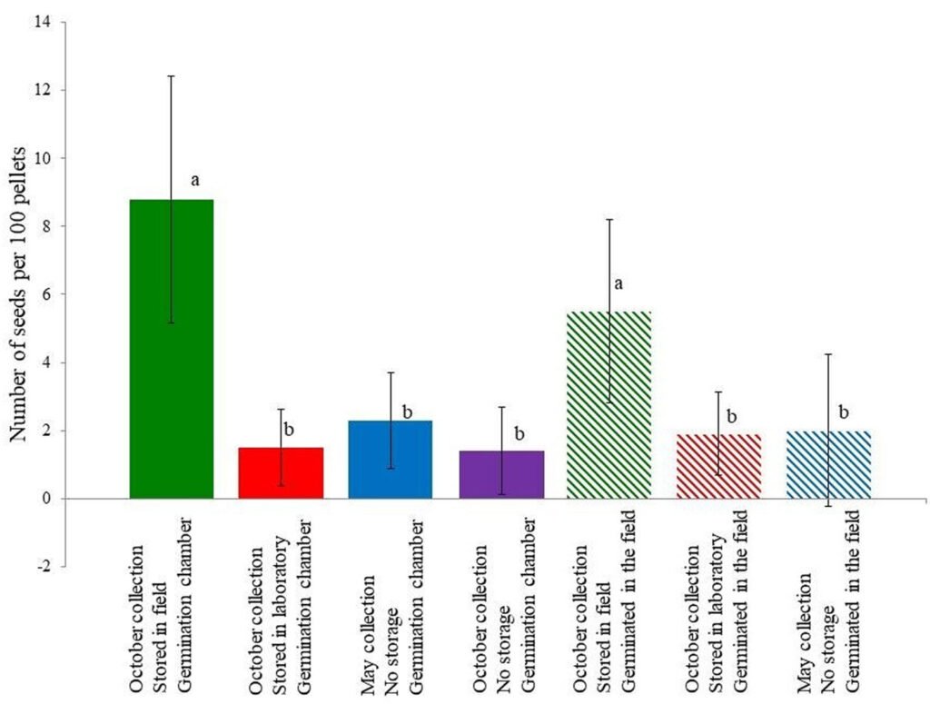
Figure 1. Number of seeds germinated per 100 cottontail fecal pellets ± standard deviation. Letters represent significant differences between treatments according to the Dunn test. Full bars represent treatments in germination chambers.
Discussion
The first experiment showed that seeds from both entire and disintegrated pellets can germinate equally well. We used disintegrated pellets in the following experiments because they are easier to homogeneously disperse in the experiment tray. However, germination was very low in the experiments with no soil. This suggests that if the pellets are placed on soil, the seeds inside are able to germinate, but if the cottontail forms a latrine on a rock or some other hard object (as it is commonly observed in our study location; pers. obs.), the pellets are not a good substrate for the plants to develop (at least in the fresh state). An interesting observation that we made was that in the October germination experiment, fungi were an important problem for plant development, but the same did not happen in the following experiment. This could be due to the fact that July-October are the months when most fungi expel their spores and infect the pellets (Valenzuela et al., 2009), but they apparently (at least partially) die before the germination period and by May do not represent an important threat for seeds or seedlings. Therefore, fungi are unlikely to strongly affect the process of seed dispersion by cottontails, since our October germination experiment would never happen in field conditions because of the dry season.
Baskin and Baskin (2014) mention that in xerophitic scrubs, 85% of seeds have some sort of dormancy; this is close to the results of our experiment. If we compare the number of seeds germinated from pellets stored in laboratory and field conditions, we can see that pellets exposed to the field yielded 5.9 (in germination chambers) and 2.9 (in the field) times more plants (Fig. 1). This suggests that most seeds have some sort of dormancy that is broken by the conditions in the field, most likely by heat, as it was shown for Opuntia tomentosa (Olvera-Carrillo et al., 2003). Notice that the Opuntia seeds almost never germinate after being stored in laboratory conditions (Table 1).
Table 1
Number and identity of the seeds germinated per 1,000 fecal pellets in each treatment. Chao estimator ± 95% confidence interval.
| Germinated in chambers | Germinated in the field | Total | |||||
| Collection | October collection | May collection | October collection | May collection | |||
| Storage | Field | Lab. | None | Field | Lab. | None | |
| Poaceae1 | 29 | 9 | 5 | 25 | 7 | 1 | 76 |
| Opuntia tomentosa | 13 | 1 | 14 | 12 | 0 | 17 | 57 |
| Physalis glutinosa | 15 | 2 | 2 | 8 | 7 | 2 | 36 |
| Jaegeria hirta | 17 | 1 | 0 | 8 | 2 | 0 | 28 |
| Drymaria laxiflora | 6 | 0 | 1 | 1 | 0 | 0 | 8 |
| Crusea longiflora | 5 | 0 | 0 | 0 | 0 | 0 | 5 |
| Jaltomata procumbens | 1 | 1 | 0 | 1 | 1 | 0 | 4 |
| Galinsoga parviflora | 1 | 0 | 0 | 0 | 0 | 0 | 1 |
| Evolvulus alsinoides | 1 | 0 | 0 | 0 | 0 | 0 | 1 |
| Bidens bigelovii | 0 | 0 | 0 | 0 | 1 | 0 | 1 |
| Solanum bulbocastanum | 0 | 1 | 0 | 0 | 0 | 0 | 1 |
| Buddleja cordata | 0 | 0 | 1 | 0 | 0 | 0 | 1 |
| Unidentified | 0 | 0 | 0 | 0 | 1 | 0 | 1 |
| Total seeds | 88 | 15 | 23 | 55 | 19 | 20 | 220 |
| Pellets used | 1,000 | 1,000 | 1,000 | 1,000 | 1,000 | 1,000 | 6,000 |
| Observed richness | 9 | 6 | 5 | 6 | 6 | 3 | 15 |
| Chao2 richness | 11.7 ± 4.1 | 10.6 ± 4.8 | 10.1 ± 6.5 | 7.9 ± 2.0 | 11.1 ± 6.5 | 3.5 ± 1.2 | 29.8 ± 13.4 |
1Includes: Aegopogon tenellus, Eragrostis Mexicana, and Chloris gayana (the last one is the only exotic species).
The Eastern cottontails showed to be poor seed dispersers if considering the amount of seeds per gram of excretes, 0.77 under the best conditions, compared with the 7.13 seeds/g of excrete dispersed by ringtails in the same location (Peña-Herrera et al., 2024). However, cottontails produce around 350 pellets/day (Cochran & Stains, 1961), which at a weight of 0.115 g/pellet (Glebskiy, 2016) which equals 40 g of excretes and thus up to 31 seeds dispersed per day per cottontail (and their population can rise up to 14 individuals/ha (Glebskiy, 2016). Another important consideration is the identity of the seeds, from the 14 species that we were able to identify; only 2 (Opuntia tomentosa and Buddleja cordata) could be considered dominant in the region (according to the list provided by Cano-Santana [1994]), and the other species are less common or even rare. Most noticeable Jaegeria hirta, which composes 12.7% of all seeds found and is a native but rare species for the location. It has to be noted that of the dispersed species (Table 1), only Chloris gayana is exotic to the location. When comparing to the seeds dispersed by ringtails in the same location (Peña-Herrera et al., 2024), we can see that only 3 species are shared (Opuntia tomentosa, Drymaria laxiflora, and Bidens sp.) and cottontails tend to disperse more Poaceae plants. This suggests that ringtails and rabbits have a complementary role as seed dispersers.
Therefore, we conclude that while being poor dispersers of seeds/g of excrete (the most commonly used estimator to measure dispersion efficiency), cottontails compensate for this by the sheer amount of excretes produced, their high population density, and the fact that they disperse mostly uncommon or even rare plants, and most are native to the region. Thus, cottontails are important seed dispersers and can have a great effect on some rare plants, especially Jaegeria hirta.
Acknowledgements
We are thankful to Díaz Rico A. and Zúñiga Ruíz B. for allowing us to use their germination chambers, Martínez Orea Y. for the plant identification, SEREPSA working team for the permits to collect pellets, List Sánches R. and Godínez Álvarez H. for their useful comments on this project, and Castellanos Vargas I. for technical support. This project was financially supported by PAPIIT grant IV200117 “Análisis ecosocial de una reserva urbana para la sustentabilidad en el campus de Ciudad Universitaria” to ZCS and a scholarship by Conacyt 817316 to YG.
References
Albert, A., Auffret, A. G., Cosyns, E., Cousins, S. A., D’hondt, B., Eichberg, C. et al. (2015). Seed dispersal by ungulates as an ecological filter: A trait-based meta-analysis. Oikos, 124, 1109–1120. https://doi.org/10.1111/oik.02512
Baskin, C. C., & Baskin, J. M. (2014). Seeds ecology, biogeography, and evolution of dormancy and germination. 2nd. Edition. San Diego: Elsevier.
Beaune, D., Bretagnolle, F., Bollache, L., Bourson, C., Hohmann, G., & Fruth, B. (2013). Ecological services performed by the bonobo (Pan paniscus): seed dispersal effectiveness in tropical forest. Journal of Tropical Ecology, 29, 367–380. https://doi.org/10.1017/S0266467413000515
Borchert, M., & Tyler, C. (2023). Fruit production and seed dispersal of Opuntia phaeacantha (Cactaceae) in the southwest Mojave Desert. Haseltonia, 29, 49–56. https://doi.org/10.2985/026.029.0108
Cano-Santana, Z. (1994). Flujo de energía a través de Sphenarium purpuracens(Orthoptera: Acrididae) y productividad primaria neta aérea en una comunidad xerófila. (Ph.D. Thesis). Mexico City: Universidad Nacional Autónoma de México.
César-García, S. F. (2002). Análisis de algunos factores que afectan la fenología reproductiva de la comunidad vegetal de la Reserva del Pedregal de San Ángel, D.F. (México) (Bachelor´s Thesis). Mexico City: Universidad Nacional Autónoma de México.
Chapman, J. A., & Flux, J. E. (2008). Introduction to the Lagomorpha. In P. C. Alves, N. Ferrand, & K. Hackländer (Eds.), Lagomorph Biology: evolution, ecology, and conservation (pp. 1–9). Berlin: Springer. https://doi.org/10.1007/978-3-540-72446-9
Chapman, J. A., Hockman, J. G., & Ojeda, C. M. M. (1980). Sylvilagus floridanus. Mammalian Species, 136, 1–8.
Cochran, G. A., & Stains, H. J. (1961). Deposition and decomposition of fecal pellets by cottontails. The Journal of Wildlife Management, 25, 432–435. https://doi.org/10.2307/3798835
Gelmi-Candusso, T. A., & Hämäläinen, A. M. (2019). Seeds and the city: the interdependence of zoochory and ecosystem dynamics in urban environments. Frontiers in Ecology and Evolution, 7, 41. https://doi.org/10.3389/fevo.2019.00041
Glebskiy, Y. (2016). Factores que afectan la distribución y abundancia del conejo castellano (Sylvilagus floridanus) en la Reserva del Pedregal de San Ángel, D.F. (México) (Bachekor’s Thesis). Mexico City: Universidad Nacional Autónoma de México.
Godó, L., Valkó, O., Borza, S., & Deák, B. (2022). A global review on the role of small rodents and lagomorphs (clade Glires) in seed dispersal and plant establishment. Global Ecology and Conservation, 33, e01982. https://doi.org/10.1016/j.gecco.2021.e01982
Hortelano-Moncada, Y., Cervantes, F. A., & Trejo-Ortiz, A. (2009). Mamíferos silvestres de la Reserva Ecológica del Pedregal de San Ángel en Ciudad Universitaria, Universidad Nacional Autónoma de México, México, D. F. Revista Mexicana de Biodiversidad, 80, 507–520. https://doi.org/10.22201/ib.20078706e.2009.002.614
Hudson, R., Rodríguez-Martínez, L., Distel, H., Cordero, C., Altbäcker, V., & Martínez-Gómez, M. (2005). A comparison between vegetation and diet records from the wet and dry season in the cottontail rabbit Sylvilagus floridanus at Ixtacuixtla, central Mexico. Acta Theriologica, 50, 377–389. https://doi.org/10.1007/BF03192633
Iluz, D. (2011). Zoochory: the dispersal of plants by animals. In Z. Dubinsky, & J. Seckbach (Eds.), All flesh is grass: plant-animal interrelationships (pp. 199–214). Dordrecht: Springer. https://doi.org/10.1007/978-90-481-9316-5_9
Lezama-Delgado, E., Sainos-Paredes, P., López-Portillo, J., Ángeles, G., Golubov, J., & Martínez, A. J. (2016). Association of Juniperus deppeana (Cupressaceae: Pinales) seeds with Mexican cottontail rabbit (Sylvilagus cunicularius; Leporidae: Lagomorpha) latrines. Journal of Natural History, 50, 2547–2555. https://doi.org/10.1080/
00222933.2016.1200685
Lorenzo, C., & Cervantes, F. (2005). Silvialgus floridanus. In G. C. G. Oliva, & G. Ceballos (Eds.), Los mamíferos silvestres de México. Mexico City: Comisión Nacional para el Conocimiento y Uso de la Biodiversidad/ Fondo de Cultura Económica.
Malo, J. E., & Suárez, F. (1995). Herbivorous mammals as seed dispersers in a Mediterranean dehesa. Oecologia, 104, 246–255. https://doi.org/10.1007/bf00328589
Olvera-Carrillo, Y., Márquez-Guzmán, J., Barradas, V. L., Sánchez-Coronado, M. E., & Orozco-Segovia, A. (2003). Germination of the hard seed coated Opuntia tomentosa
SD, cacti from the México valley. Journal of Arid Environments, 55, 29–42. https://doi.org/10.1016/s0140-1963(02)00268-9
Peña-Herrera, J. J., Glebskiy, Y., Hernández-Trejo, T., & Cano-Santana, Z. (2024). Ringtails (Bassariscus astutus) as seed dispersers in an urban gradient under conditions of low human activity due to COVID-19. Revista Mexicana de Biodiversidad, 95, e955351. https://doi.org/10.22201/ib.20078706e.2024.95.5351
Rosin, A. V., Gilio, N., & Meriggi, A. (2008). Introduced lagomorphs as a threat to “native” lagomorphs: the case of the Eastern cottontail (Sylvilagus floridanus) in northern Italy. In P. C. Alves, N. Ferrand, & K. Hackländer (Eds.), Lagomorph Biology: evolution, ecology, and conservation (pp. 153–164). Berlin: Springer. https://doi.org/10.1007/978-3-540-72446-9_11
Rzedowski, J. (1954). Vegetación del Pedregal de San Ángel. Anales de la Escuela Nacional de Ciencias Biológicas, Instituto Politécnico Nacional, 8, 59–129.
SMN (Servicio Meteorológico Nacional). (2025). Normales climatológicas 1991-2020, estación 9071 Colonia Educación. https://smn.conagua.gob.mx/tools/RESOURCES/Nor
males_Climatologicas/Normales9120/df/nor9120_09071.txt
Valenzuela, V. H., Herrera, T., & Pérez-Silva, E. (2009). Macromicetos. In A. Lot, & Z. Cano-Santana (Eds.), Biodiversidad del ecosistema del Pedregal de San Ángel (pp. 95–100). Mexico City: Universidad Nacional Autónoma de México.

Crecimiento, edad y tasa de mortalidad de la estrella de mar corona de espinas Acanthaster plancien el sur del golfo de California, México, durante un evento de explosión poblacional (2017-2018)
Growth, age and mortality rate of the crown-of-thorns starfish, Acanthaster planci, in the southern gulf of California, Mexico, during an outbreak event (2017-2018)
Héctor Reyes-Bonilla a, Frida J. Sánchez-Luna b, c, Luis E. Calderón-Aguilera d, *, Jenny Carolina Rodríguez-Villalobos e, f y María Dinorah Herrero-Pérezrul e
a Universidad Autónoma de Baja California Sur, Departamento Académico de Biología Marina, Carretera al sur Km 5.5, Col. El Mezquitito, 23090 La Paz, Baja California Sur, México
b Ghent University, Faculty of Sciences, Krijgslaan 281/N60, 9000 Gent, Bélgica
c Università Politecnica delle Marche, Via, Dipartimento di Scienze della Vita e dell’Ambiente, Brecce Bianche, 60131 Ancona, Italia
d Centro de Investigación Científica y de Educación Superior de Ensenada, Baja California, Carretera Tijuana – Ensenada 3918, 22860 Ensenada, Baja California, México
e Centro Interdisciplinario de Ciencias Marinas, Instituto Politécnico Nacional, Av. Instituto Politécnico Nacional s/n, Col. Playa Palo de Santa Rita, 23096 La Paz, Baja California Sur, México
f Ecosistemas y Conservación (Proazul Terrestre, A.C.), calle Héroes de Independencia 2440, 23000 La Paz, Baja California Sur, México
*Autor de correspondencia: leca@cicese.mx (L.E. Calderón-Aguilera)
Recibido: 18 febrero 2025; aceptado: 22 octubre 2025
Resumen
El asteroideo Acanthaster planci es un importante coralívoro y se requiere investigar en detalle aspectos de su ecología poblacional. El objetivo del estudio fue estimar parámetros demográficos de A. planci en el archipiélago Espíritu Santo, golfo de California. Entre julio 2017 y octubre 2018 se midió el diámetro del disco de 356 especímenes y con base en análisis de frecuencia de tallas, se calculó el diámetro de disco máximo teórico, la tasa de crecimiento y mortalidad, y la longevidad de la población. El tamaño máximo del disco fue de 30.8 cm, la tasa de crecimiento de 0.429/año, la longevidad de 6 años y la tasa de mortalidad fue de 1.039/año. La edad de los individuos revisados en 2017 fluctuó entre 1.0 y 1.25 años, y en 2018 fue de 1.75 a 2.25 años, lo que sugiere que la cohorte de 2016 causó el notable aumento poblacional registrado para A. planci en 2017. Este evento pudo haber resultado de la combinación del alto reclutamiento larval favorecido por el agua cálida aportada por el evento de El Niño de 2015 y una alta sobrevivencia de juveniles debido a la presencia de abundante alimento algal como consecuencia de La Niña en 2016.
Palabras clave: Frecuencia de tallas; FISAT; Mortalidad; Crecimiento; Reclutamiento; Brote poblacional
Abstract
The asteroid Acanthaster planci is an important corallivore, and the investigation of some aspects of its population ecology are required. The objective of this study was to estimate demographic parameters of A. planci at Espíritu Santo Archipelago, Gulf of California. Between July 2017 and October 2018, the disk diameter of 356 specimens was measured, and with these data the theoretical maximum diameter, growth and mortality rates, and longevity of the population were estimated on the basis of size frequency analyses. The maximum disk size was 30.8 cm, growth rate was 0.429 yr-1, longevity was 6 years, and mortality rate was 1.039 yr-1. Age of the individuals assessed in 2017 fluctuated between 1.0 and 1.25 years, and in 2018 was from 1.75 to 2.25 years, which suggests that the 2016 cohort caused a noteworthy population to increase recorded for A. planci in 2017. This event may have resulted from the combination of high larval recruitment favored by the warm water brought by the 2015 El Niño, and high juvenile survival due to abundant algal food as consequence of La Niña in 2016.
Keywords: Length frequency; FISAT; Mortality; Growth; Recruitment; Outbreak
Introducción
La estrella corona de espinas (Acanthaster spp.) es uno de los equinodermos que ha sido más estudiado en arrecifes del Indo-Pacífico debido al interés que genera el incremento excesivo en la densidad de sus poblaciones. Cuando ésto ocurre, la intensidad de la depredación de la estrella sobre los corales supera las tasas de crecimiento de las colonias y el asteroideo se convierte en una de las mayores amenazas para los arrecifes coralinos (De’ath et al., 2012; Kayal et al., 2012; Pratchett et al., 2014). Hasta la fecha (septiembre 2025), de acuerdo con el Registro Mundial de Especies Marinas (World Register of Marine Species; WoRMS: https://www.marinespecies.org/aphia.php?p=taxdetailsyid=205212), se reconocen 4 especies pertenecientes al género Acanthaster: A. planci (Linneo, 1758), A. mauritiensis de Loriol, 1885, A. brevispinus, Fisher, 1917 y A. benziei Worheide, Kaltenbaher, Cowan y Hazprunar, 2022, aunque estudios genéticos apuntan a que A. planci en realidad es un complejo de posiblemente 5 taxones (Hazprunar y Spies, 2014), y refieren que la especie presente en la costa del Pacífico de América podría ser Acanthaster sp. cf. solaris Schreber, 1793. Aunque este último nombre se ha usado en publicaciones recientes relativas a la ecología de Acanthaster en el Pacífico oriental (Martínez-Sarabia y Reyes-Bonilla, 2021; Rodríguez-Villalobos y Ayala-Bocos, 2018, 2021), la discusión sigue activa y por motivos de estabilidad taxonómica, en el presente trabajo se decidió utilizar el nombre de A. planci para referirse a la especie de interés.
A pesar de su presencia en los arrecifes rocosos y coralinos de la región del Pacífico oriental tropical, la estrella no ha recibido demasiada atención quizás debido a sus densidades relativamente bajas (Enochs y Glynn, 2017; Reyes-Bonilla y Calderón-Aguilera, 1999; Rodríguez-Villalobos et al., 2016), así como a la poca evidencia de daño masivo sobre los corales (Rodríguez-Villalobos et al., 2015). Sin embargo, Rodríguez-Villalobos y Ayala-Bocos (2018, 2021) señalaron que en 2017 hubo un incremento abrupto en la densidad de los individuos de esta especie en el Parque Nacional Zona Marina del Archipiélago Espíritu Santo (PNZMAES) acompañado por la mortalidad masiva de colonias de coral de los géneros Pocillopora, Porites y Pavona. Este evento tuvo efectos importantes sobre las comunidades coralinas e incluso afectó esfuerzos de restauración que se estaban llevando a cabo en la misma región (Martínez-Sarabia y Reyes-Bonilla, 2021).
Las causas del incremento de A. planci en el sur del golfo de California son desconocidas. En el Indo-Pacífico las fluctuaciones del tamaño de la población de la estrella se han relacionado con condiciones ambientales como aumentos de temperatura, alta concentración de clorofila y baja salinidad (Fabricius et al., 2010; Hoegh-Guldberg y Pearse, 1995; Lamare et al.,2014). Aunque hasta el momento no hay una explicación universal para la formación de brotes poblacionales (Babcock et al., 2016), el fenómeno debe estar relacionado con las características biológicas de la estrella, tales como alto potencial reproductivo y fecundidad, buena sobrevivencia larval y reclutamiento de individuos, sistemas defensivos en su fase adulta (que incluyen espinas, saponinas y compuestos alelopáticos), y alta capacidad competitiva; además, existen pocos depredadores naturales que controlen el crecimiento de sus poblaciones (Pratchett et al., 2014).
A partir de la observación del aumento anómalo de su abundancia en la región sur del golfo de California y para tener mejores herramientas para el manejo del problema, surgió la interrogante de conocer la estructura de edades de A. planci en la región para elucidar la posible relación del incremento de abundancia con un pulso previo de alto reclutamiento. Así, el objetivo de este trabajo fue obtener los parámetros de la ecuación de crecimiento para una población de A. planci en fase explosiva y calcular la edad relativa de los organismos, además de la tasa de mortalidad natural.
Materiales y métodos
El archipiélago Espíritu Santo se encuentra al oriente de la bahía de La Paz (24º28’17” N, 110º19’57” O; fig. 1). Topográficamente, el litoral oriental de la isla es rocoso y homogéneo, mientras que la costa occidental cuenta con entrantes y salientes que forman zonas protegidas. Las zonas someras en el lado oeste de Espíritu Santo permiten la formación de arrecifes rocosos con la presencia de parches coralinos distribuidos de manera discontinua (Reyes-Bonilla y López-Pérez, 2009). Se registran temperaturas mínimas de 20 ºC a finales del invierno (febrero) y máximas de 30 ºC a mediados del verano (agosto). Adicionalmente, se observan corrientes de menor intensidad en la parte norte y de mayor intensidad en la parte sur (canal de San Lorenzo) (Conanp, 2018).
Se visitaron 10 localidades en el archipiélago (fig. 1) en julio y agosto de 2017, y en septiembre y octubre de 2018 para determinar la abundancia y el diámetro del disco (en cm) de todos los ejemplares de la estrella que se encontraban dentro de transectos de banda de 25 x 3 m, desplegados en paralelo a la línea de costa a una profundidad de 2 a 10 m. Para estimar la tasa de crecimiento y de mortalidad, se empleó el paquete FISAT II (FAO-ICLARM Fish Stock Assessment Tools versión 1.2.2). Se decidió aplicar la curva de crecimiento de von Bertalanffy (Haddon, 2011), ya que Pratchet et al. (2014), después de un análisis de los diversos trabajos al respecto, indican que este es el modelo que mejor expresa el crecimiento de Acanthaster a partir del segundo año de vida.
Para la aplicación del modelo, la talla máxima teórica L∞ fue calculada empleando la técnica de Powell-Wetherall (Haddon, 2011), la cual parte de la suposición que la población está en estado estable (tasa de mortalidad proporcional a la tasa de reclutamiento), y se fundamenta en las siguientes ecuaciones:
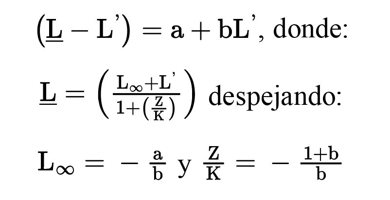
Por otra parte, la tasa de crecimiento K se obtuvo con el método de Shepherd (Haddon, 2011), el cual busca maximizar una función no paramétrica S, que se define como
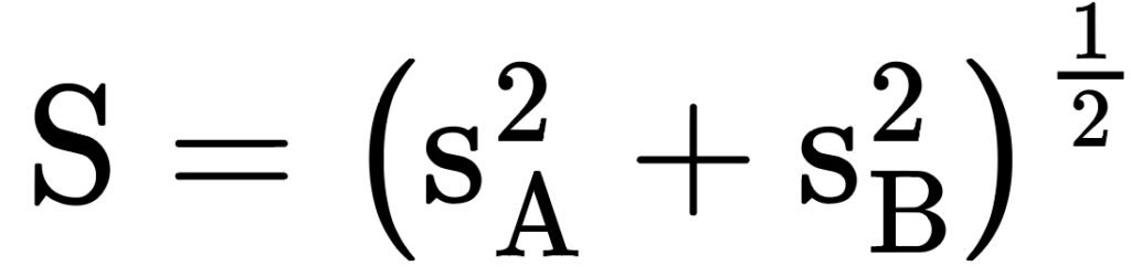
donde SAy SB son los valores de bondad de ajuste (“scores”) obtenidos en tiempo calendario (stz) para SA = 0 y SB = 0.25 años a partir del origen de la curva de crecimiento de VB. Las ecuaciones aplicadas son:
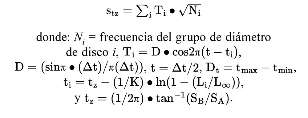
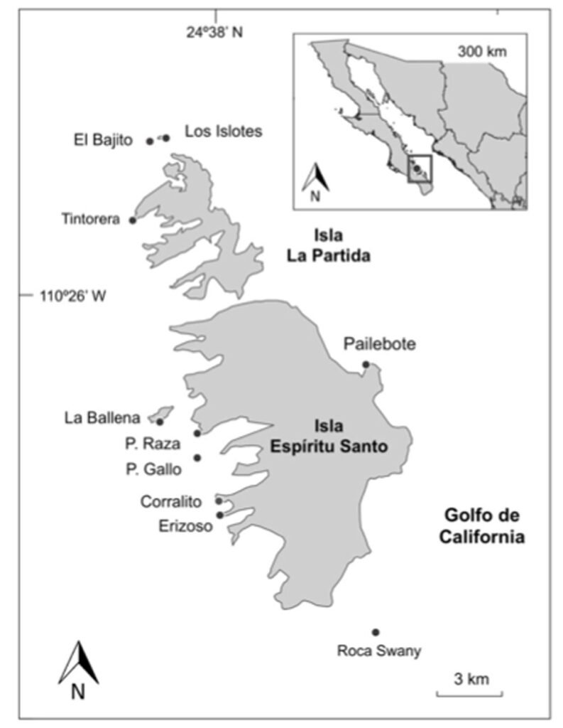
Figura 1. Localización de los puntos de muestreo para la determinación de tallas de Acanthaster planci en el Parque Nacional Zona Marina del Archipiélago Espíritu Santo (PNZMAES).
Una vez con los parámetros L∞ y K, se procedió a trazar la curva teórica de crecimiento de la especie (expresando el diámetro en cm en relación con la edad del organismo en intervalos de 0.25 años) a construir la tabla diámetro de disco-edad, con lo cual se determinó la edad de los individuos muestreados en 2017 y 2018. Tomando en cuenta que los estudios previos sobre crecimiento de la estrella corona de espinas han sido hechos con base en el diámetro total de los individuos (Zann et al., 1987), se trazó una curva teórica para evaluar el crecimiento en esta dimensión, considerando que Glynn (1982) determinó que el diámetro total de Acanthaster en Panamá podría ser aproximado a partir del diámetro del disco ya que este representa 56% del total.
Finalmente, para calcular la tasa de mortalidad de la población (M) de especies a las que no se les puede asignar directamente la edad con base en estructuras óseas u otros procedimientos, se emplean ecuaciones empíricas o basadas en aspectos teóricos del crecimiento de organismos marinos (Sparre y Venema, 1995). La bibliografía cita el uso de diversas metodologías para evaluar este parámetro en equinodermos comerciales (Herrero-Pérezrul y Chávez, 2005; Reyes-Bonilla y Herrero-Pérezrul, 2003), pero para el caso de Acanthaster no todas son aplicables ya que su uso requiere información no disponible; por ejemplo, la ecuación de Rikhter y Efanov utilizada por Penchaszadeh y Molinet (2020), necesita la edad de primera madurez (la cual es desconocida para Acanthaster en el Pacífico americano), mientras que métodos como el de Beverton y Holt (Sparre y Venema, 1995) solo son aplicables a especies de consumo humano porque requieren datos de talla de primera captura. Por lo anterior, se decidió estimar valores de M usando 3 métodos: la ecuación de Pauly (1984) basada en la temperatura promedio local (25 °C) y el valor de L∞ y K; la de Jensen (1997), fundamentada en el valor de K; y la curva de captura de Ricker (1975), obtenida de la frecuencia de individuos y sus respectivas edades estimadas.
Resultados
Se midieron 356 individuos de A. planci en 2017 y 2018. Los especímenes de 2017 fueron en promedio 5.5 cm más pequeños que los de 2018 (tabla 1, fig. 2; t de Student para varianzas desiguales t318 = 13.413, p < 0.001). La distribución de tallas de los individuos se presenta en las figuras 2 y 3, y puede observarse que en 2017 solamente un individuo alcanzó un diámetro de disco superior a 20 cm, mientras que en el año siguiente 21 de 227 organismos (9.3%) superan ese umbral. En 2017, 9% de las estrellas fueron menores a 8 cm de diámetro.
A partir de los análisis de tallas, el diámetro máximo de disco estimado para la población de Acanthaster estudiada (L∞) fue de 30.8 cm mientras que su tasa anual de crecimiento (K) fue de 0.429∙año-1. La ecuación de crecimiento toma entonces la siguiente forma:
Lt = 30.8 * (1 – e [-0.429* (t – 0.01)]),
donde: Lt = diámetro de disco (en cm) a la edad t y t = edad (años).
Los organismos crecen rápidamente de tal modo que al final del año 1 cuentan con 10.7 cm de diámetro de disco, para el año 2 alcanzan 17.7 cm, y para el 3 llegan a 22.2 cm. El modelo teórico junto con la edad estimada de los individuos se presenta en la figura 4. Para facilitar comparaciones con otras publicaciones donde se hace referencia a la talla de A. planci en el Pacífico americano y donde la medida de los organismos se hizo tomando en cuenta el diámetro total, en la figura 5 se presenta la curva teórica de crecimiento aquí generada y la esperada para el diámetro total, considerando que el diámetro del disco representa 55% del diámetro total de la estrella según Glynn (1982).
La estructura esperada de edades para los años 2017 y 2018 a partir de la ecuación de von Bertalanffy y calculada con el diámetro del disco, se presenta en la figura 6. Se observa que la edad predominante en el primer año de muestreo fue entre 1 y 1.5 años (a partir de julio), indicando que los individuos posiblemente se reclutaron a finales de 2015. Esto es corroborado en la figura 6, ya que para 2018 hubo una alta frecuencia de animales con edades de 1.75 a 2.25 años.
Tabla 1
Estadísticos descriptivos (en cm) del diámetro del disco de la población de Acanthaster planci estudiada en el Parque Nacional Zona Marina del Archipiélago Espíritu Santo (PNZMAES) en 2017 y 2018.
| Estadístico | 2017 | 2018 | Ambos años |
| Promedio | 11.43 | 16.96 | 14.96 |
| Desviación típica | 5.44 | 4.28 | 4.78 |
| Error típico | 0.29 | 0.23 | 0.25 |
| Moda | 11 | 16 | 16.0 |
| Mediana | 10.9 | 16.5 | 15.0 |
| Máximo | 23.3 | 28.0 | 28.0 |
| Mínimo | 3.8 | 5.2 | 3.8 |
| N | 129 | 227 | 356 |
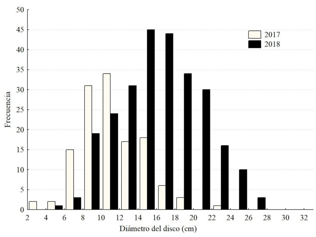
Figura 2. Histogramas del diámetro del disco (en cm) para la población de Acanthaster planci en el Parque Nacional Zona Marina del Archipiélago Espíritu Santo (PNZMAES) durante los años 2017 y 2018.
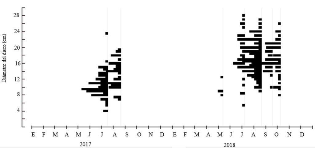
Figura 3. Frecuencia de diámetro del disco de Acanthaster planci en el Parque Nacional Zona Marina del Archipiélago Espíritu Santo (PNZMAES) durante los años 2017 y 2018.
Por último, la tasa anual de mortalidad esperada para la población de A. planci analizada, dependiendo del método indirecto aplicado, fue de 1.0392 (ecuación de Pauly), 0.3983 (curva de captura) y 0.6433 (ecuación de Jensen), con un promedio de 0.6936∙año-1. La mortalidad en el año 1 es alta, ya que el método que arrojó los valores más conservadores (Ricker) indica pérdidas de 33% de la cohorte teórica, mientras que el método de Pauly indica que apenas sobrevive 35%. Al tomar en cuenta el valor promedio de las 3 estimaciones del parámetro M, para el año 1 sobrevive 49.9% de la cohorte, para el año 3 apenas 12.5% de los individuos originales permanece y solo 3.1% alcanza la edad de 5 años. Estos valores se reflejan en los histogramas de edad (fig. 6) donde la edad máxima observada (5.75 años) fue de un individuo de 28 cm.
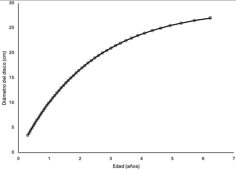
Figura 4. Curva talla-edad de Acanthaster planci en el Parque Nacional Zona Marina del Archipiélago Espíritu Santo (PNZMAES, n = 356).
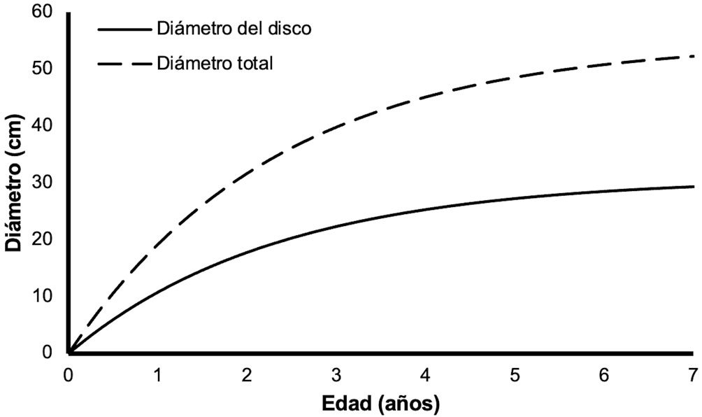
Figura 5. Curvas de crecimiento individual de Acanthaster planci en el Parque Nacional Zona Marina del Archipiélago Espíritu Santo (PNZMAES). La línea puntuada representa la curva extrapolada a partir de la ecuación de Glynn (1982).
Discusión
Este es el primer estudio de crecimiento de Acanthaster planci en el Pacífico oriental y uno de los pocos a escala mundial (MacNeil et al., 2017; Pratchett et al., 2014; Zann et al., 1987). El cálculo de los parámetros de crecimiento de esta especie ha sido difícil de realizar especialmente porque los marcajes en campo para hacer seguimiento de tallas a lo largo del tiempo no han sido exitosos, ya que los individuos eliminan los colorantes o autotomizan la espina o incluso el brazo donde se coloca la marca (Chim y Tan, 2013; MacNeil et al., 2016; Pratchett et al., 2014). Además, en el caso del continente americano, otro motivo que hace complicado conducir estudios demográficos es que las poblaciones son relativamente pequeñas (menos de 70 ind/ha, equivalente a encontrar 1 individuo cada 142.8 m2, según Rodríguez-Villalobos et al. [2021]), lo cual hace complejo tener tamaños de muestra adecuados para realizar análisis en detalle.
Para solucionar ésto, la mayor parte de los trabajos sobre crecimiento de Acanthaster se han basado en especímenes mantenidos en confinamiento (Lucas, 1984; Yamaguchi, 1974; Zann et al., 1987), pero por las dificultades logísticas que implica mantener ejemplares a largo plazo, los experimentos no han durado más de 1 o 2 años. Otra opción para estimar la edad de Acanthaster ha sido la relación entre el número de anillos de las espinas (tomado como indicador indirecto de la edad) y el diámetro total medido en el campo (MacNeil et al., 2017; Stump, 1996), pero la debilidad de estos estudios radica en que no se ha logrado demostrar que los anillos sean anuales. Finalmente, Kenchington (1977) empleó información de 10 años de mediciones de organismos en la Gran Barrera Arrecifal y a partir de cambios en las modas estimó que a la edad de 3 años un individuo podrá superar los 30 cm de diámetro máximo; es decir, el autor empleó un método indirecto similar al utilizado en el presente trabajo. En resumen, los métodos empleados en esta investigación permiten alcanzar estimaciones de crecimiento con una precisión muy semejante a las que se han obtenido en otras partes del mundo, por lo que los resultados obtenidos son confiables.
La talla promedio que se observó tomando en cuenta los años 2017 y 2018 (14.96 + 0.25 cm; tabla 1) frecuentemente se observa en individuos residentes de los arrecifes del Pacífico oriental tropical (Glynn, 1982; Narváez y Zapata, 2010), pero muy inferior a la que se alcanza en el Indo-Pacífico (MacNeil et al., 2016; Mendonça et al., 2010). Esta diferencia se puede explicar con base en los argumentos de Kettle y Lucas (1987) y Hernández-Morales et al. (2021), quienes anotan que la talla de Acanthaster es proporcional a la calidad del alimento consumido, por lo que el pequeño tamaño de los individuos en la zona de estudio y a lo largo del Pacífico oriental tropical se puede deber a que las poblaciones de la estrella corona de espinas tienen una dieta pobre, probablemente debido a que la cobertura y diversidad de corales para alimentarse es mucho menor que en el resto del Pacífico.
Aunque existen diferencias notables tanto en las tallas alcanzadas por Acanthaster en distintas regiones como en las metodologías aplicadas para determinar su curva de crecimiento, los estudios llevados a cabo en Australia muestran que en el primer año de vida esta especie normalmente no alcanza los 5 cm de diámetro total, pero su crecimiento es muy rápido durante el segundo año, alcanzando entre 12.5 y 25 cm, y para el año 3 puede llegar a los 35 cm de diámetro máximo (MacNeil et al., 2017; Pratchett et al., 2014; Zann et al., 1987). Estos hallazgos presentan cierta discrepancia en relación con la talla esperada en el archipiélago Espíritu Santo a un año (fig. 5), la cual es de más de 19 cm de diámetro total, de acuerdo con la corrección sugerida por Glynn (1982). Kenchington (1977), empleando un método de progresión modal, también sugirió que Acanthaster puede alcanzar hasta 12 cm de diámetro máximo para el año 1, pero esa cifra sigue siendo baja comparada con la aquí presentada. Considerando lo anterior, es posible que, como sugieren Pratchett et al. (2014), aunque el modelo de crecimiento de von Bertalanffy es robusto en general y aplicable para describir la relación entre talla y edad de organismos adultos de Acanthaster, no es muy apropiado para determinar la edad de individuos pequeños. Esto se debe a que durante su primer año, la estrella corona de espinas tiene tasas lentas de desarrollo debido a que se alimenta principalmente de algas (Kamya et al., 2017); posteriormente, pasando los 10 cm de diámetro (año 2), los ejemplares comienzan a alimentarse de coral y aceleran notablemente su crecimiento, de acuerdo con Kettle y Lucas (1987).
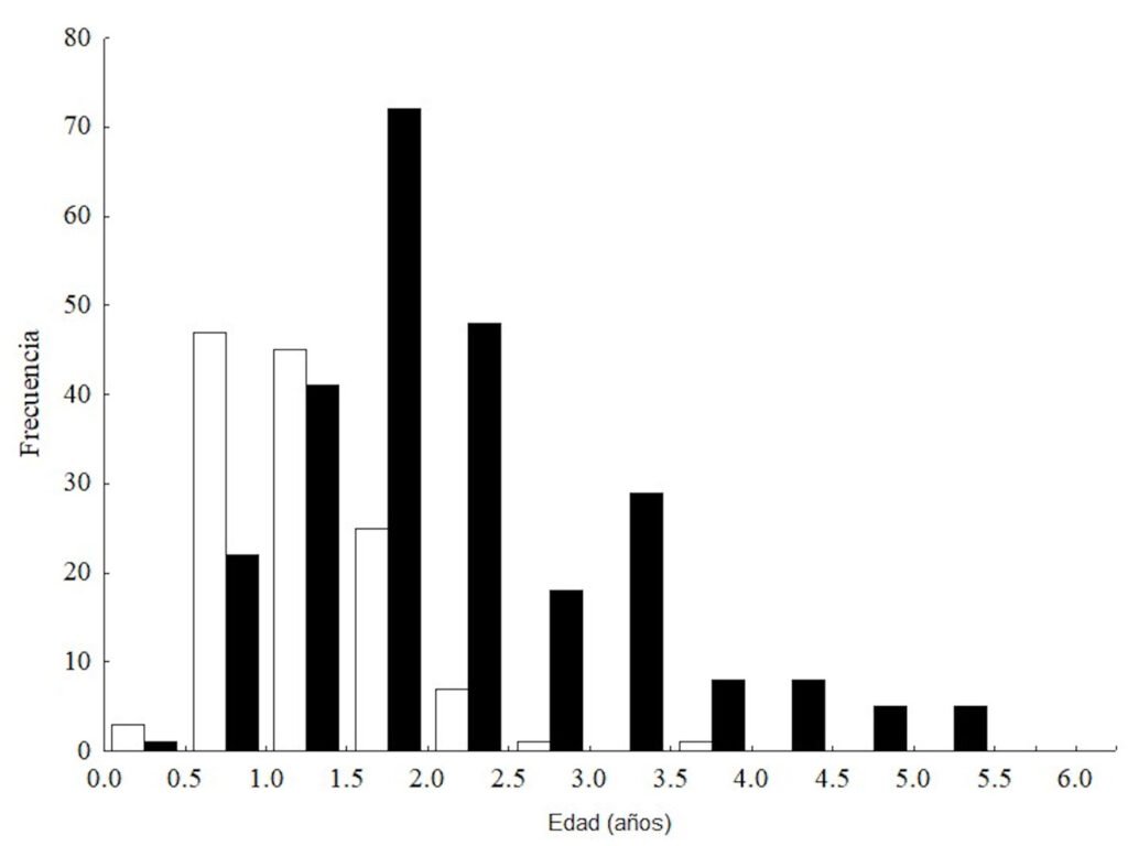
Figura 6. Estructura de edades calculada para los individuos de Acanthaster planci muestreados en 2017 y 2018 en el Parque Nacional Zona Marina de la Isla Espíritu Santo (PNZMAES).
La tasa anual de crecimiento encontrada (K) en este estudio fue de 0.429 año-1, muy similar a la reportada por MacNeil et al. (2017) de 0.54. Los valores en sí no son comparables dado que se emplearon distintas metodologías, por lo que la discusión no puede extenderse más allá de denotar la similitud. Por otra parte, la talla máxima teórica (L∞) del disco de Acanthaster en el PNZMAES fue de 30.8 cm, cercana a la presentada por MacNeil et al. (2017) de 34.9 cm a partir de un modelo bayesiano de Bertalanffy y ambas son mucho más altas que la de 20.2 cm reportada por Zann et al. (1987) en condiciones experimentales y con individuos a los que se les proporcionaron dietas de baja calidad. Usando el factor de corrección propuesto por Glynn (1982), el disco de 30.8 cm se traduce a un diámetro total de 56 cm y ello indica que teóricamente los ejemplares del golfo de California pueden alcanzar los tamaños registrados por Stump (1996) y Pan et al. (2010) en Australia y Japón (58 y 47.4 cm, respectivamente) y por Byrne et al. (2017) en la Gran Barrera Arrecifal (40 cm pero hasta 70 cm de diámetro máximo).
Además de generar el modelo de crecimiento, otro objetivo de este trabajo fue generar insumos para tratar de explicar la causa del fenómeno de explosión poblacional observado para Acanthaster en el PNZMAES durante 2017 y 2018. A este respecto y con base en la relación talla-edad, los histogramas (fig. 6) muestran que el reclutamiento de los individuos debió haber ocurrido en 2015, año durante el cual la zona se vio impactada por uno de los eventos de oscilación sureña de El Niño más fuertes en lo que va del siglo XXI y el cual afectó a los arrecifes de coral del Pacífico oriental y a las especies asociadas (Cruz-García et al., 2020; Riegl et al., 2019). La anomalía térmica alcanzada en la región de la bahía de La Paz fue superior a 2 °C (Coria-Monter et al., 2018) y alteró la ecología de todo tipo de organismos, desde mamíferos marinos hasta elementos del plancton (Elorriaga-Verplancken et al., 2016; Portner et al., 2022). Por el contrario, al año siguiente (2016-2017) la región del golfo de California estuvo influenciada por un evento de La Niña que favoreció la alta concentración de clorofila a en la columna de agua, la presencia de surgencias y aumentó la productividad (Farach-Espinosa et al., 2021).
Considerando lo anterior, es posible hipotetizar las causas del evento de explosión poblacional. Dado que las altas temperaturas aumentan la sobrevivencia larval y de los juveniles de Acanthaster (Hughes et al., 2014; Lamare et al., 2014, Pratchett et al., 2017), las anomalías térmicas de la región sur del golfo de California en 2015, combinadas con la enorme fecundidad de la estrella (más de 50 millones de huevos por individuo; Conand, 1984; Hughes et al., 2014), debieron favorecer un reclutamiento masivo. Posteriormente, las condiciones frías y productivas en el año 2016 pudieron aumentar la sobrevivencia de los juveniles al impulsar un mejor crecimiento algal en el fondo arrecifal (Wolfe et al., 2017). Así, para el año 2017 los organismos ya tenían tallas fácilmente detectables en el campo y comenzaron a realizar sus actividades de depredación, las cuales causaron notables daños a las comunidades de coral de la zona de estudio ese año (Rodríguez-Villalobos y Ayala-Bocos, 2018).
La hipótesis anterior se sustenta por los datos del modelo de edad y también por las tallas observadas en el campo. Los diámetros de disco esperados para los ejemplares (promedios de 11.43 ± 0.29 cm en 2017 y 16.96 ± 0.23 cm en 2018; tabla 1) coinciden con los reportados por Rodríguez-Villalobos y Ayala-Bocos (2021) para la zona de El Corralito en la isla Espíritu Santo (fig. 1) en 2017 (14.72 ± 2.85 cm de diámetro), lo que indica que para ese año la población de Acanthaster en la zona de estudio estaba compuesta fundamentalmente de individuos menores a 3 años, nacidos en 2015-2016 (fig. 6).
Finalmente, el modelo de sobrevivencia indica que un porcentaje muy elevado de los reclutas desaparece en el primer año de vida. Varios estudios han indicado que la tasa de mortalidad de los juveniles de Acanthaster es muy elevada (Fabricius et al., 2010; Nakamura et al., 2014; Zann et al., 1987), aunque la estimación en campo de este parámetro es notablemente difícil de obtener ya que los individuos recién reclutados de la estrella son crípticos (Fabricius, 2013). La longevidad esperada en el archipiélago Espíritu Santo fue de aproximadamente 6 años, lo cual corresponde bien a lo reportado por otros autores en Australia que indican entre 4 y 9 años de vida (Lucas, 1984; Pratchett et al., 2014). Tomando en cuenta este dato clave, es probable que la mayor parte de la cohorte de 2015 que causó el evento de mortalidad coralina masiva ya no estuviera presente en los arrecifes de la zona de estudio después del año 2021, lo cual fue confirmado a partir de datos de censos (densidades de 0.27 ind/50m2 en 2017-2018 bajó a 0.19 ind/50m2 en 2023-24). Esto implica que la población de la estrella de mar corona de espinas en el sur del golfo de California se comportó siguiendo el modelo de “aumento-caída”, típico de la especie en el Indo-Pacífico y de otros equinodermos con larvas planctotróficas (Uthicke et al., 2009).
Agradecimientos
A las autoridades y el personal del PNZMAES por las facilidades logísticas. A los miembros del staff y estudiantes asociados a la Sociedad de Historia Natural Niparajá, A.C., al personal del Laboratorio de Sistemas Arrecifales (UABCS) y a Arturo Ayala Bocos que apoyaron en las labores de campo. Las observaciones y comentarios de un revisor anónimo y del editor de la Revista Mexicana de Biodiversidad fueron clave para mejorar la presentación de las ideas y fortalecer la calidad del manuscrito.
Referencias
Babcock, R. C., Dambacher, J. M., Morello, E. B., Plagányi, É. E., Hayes, K. R., Sweatman, H. P. A. et al. (2016). Assessing different causes of Crown-of-Thorns starfish outbreaks and appropriate responses for management on the Great Barrier Reef. Plos One, 11, e0169048. https://doi.org/10.1371/journal.pone.0169048
Barham, E. G., Gowdy, R. W. y Wolfson, F. H. (1973). Acanthaster (Echinodermata, Asteroidea) in the Gulf of California. Fishery Bulletin, 71, 927–942.
Byrne, M., Rowe, F. W., Marsh, M. L. y Mah, L. C. (2017). Class Asteroidea. En: O’Hara, T. y Byrne, M. (Eds.), Australian echinoderms: biology, ecology and evolution (pp. 231–294). Melbourne: CSIRO publishing, Clayton South, Australia.
Chim, C. K. y Tan, K. S. (2013). A method for the external attachment of acoustic tags on sea stars. Journal of the Marine Biology Association of the United Kingdom, 93, 267–272. https://doi.org/10.1017/S0025315411002128
Conanp (Comisión Nacional de Áreas Naturales Protegidas). (2018). Programa de Manejo Parque Nacional exclusivamente la zona marina del Archipiélago de Espíritu Santo. Disponible en: https://www.gob.mx/publicaciones/es/articulos/parque-nacional-exclusivamente-la-zona-marina-del-archipielago-de-espiritu-santo?idiom=es
Conand, C. (1984). Distribution, reproductive cycle and morphometric relationships of Acanthaster planci (Echinodermata: Asteroidea) in New Caledonia, western tropical Pacific. Proceedings of the 5th International Echinoderm Conference, Galway, 1, 499–506.
Coria-Monter, E., Monreal-Gómez, M. A., de León, D. A. S. y Durán-Campos, E. (2018). Impact of the “Godzilla El Niño” Event of 2015-2016 on sea-surface temperature and chlorophyll-a in the southern Gulf of California, Mexico, as evidenced by satellite and in situ data. Pacific Science, 72, 411–422. https://doi.org/10.2984/72.4.2
Cruz-García, R., Rodríguez-Troncoso, A. P., Rodríguez-Zaragoza, F. A., Mayfield, A. y Cupul-Magaña, A. L. (2020). Ephemeral effects of El Niño southern oscillation events on an eastern tropical Pacific coral community. Marine Freshwater Research, 71, 1259–1268. https://doi.org/10.1071/MF18481
Dana, T. y Wolfson, A. (1970). Eastern Pacific Crown-of-thorns starfish populations in the lower Gulf of California. San Diego Society of Natural History, 16, 83–90. https://doi.org/10.5962/bhl.part.15455
De’ath G., Fabricius, K. E., Sweatman, H. y Puotinen, M. (2012). The 27-year decline of coral cover on the Great Barrier Reef and its causes. Proceedings of the National Academy of Sciences of the Unites States of America, 109, 17995–17999. https://doi.org/10.1073/pnas.1208909109
Elorriaga-Verplancken, F. R., Rosales-Nanduca, H. y Robles-Hernández, R. (2016). Unprecedented records of Guadalupe fur seals in La Paz Bay, Southern Gulf of California, Mexico, as a possible result of warming conditions in the northeastern Pacific. Aquatic Mammals, 42, 261–267. https://doi.org/10.1578/AM.42.3.2016.261
Enochs, I. C. y Glynn, P. W. (2016). Corallivory in the eastern Pacific. En Glynn, P. W., Manzello, D. y Enochs, I. C. (Eds.), Coral reefs of the Eastern Tropical Pacific: persistence and loss in a dynamic environment (pp. 315–337). Dordrecht: Springer Netherlands. https://doi.org/10.1007/978-94-017-7499-4_10
Fabricius, K. (2013). Acanthaster planci. En J. M. Lawrence (Eds.), Starfish: Biology and ecology of the Asteroidea (pp. 132–141). Baltimore: The Johns Hopkins University Press.
Fabricius, K. E., Okaji, K. y De’ath, G. (2010) Three lines of evidence to link outbreaks of the crown-of-thorns sea star Acanthaster planci to the release of larval food limitation. Coral Reefs, 29, 593–605. https://doi.org/10.1007/s00338-010-0628-z
Farach-Espinoza, E. B., López-Martínez, J., García-Morales, R., Nevárez-Martínez, M. O., Lluch-Cota, D. B. y Ortega-García, S. (2021). Temporal variability of oceanic mesoscale events in the Gulf of California. Remote Sensing, 13, 1774. https://doi.org/10.3390/rs13091774
Fisheries and aquaculture software. FISAT II – FAO-ICLARM Stock Assessment Tool. En FAO Fisheries and Aquaculture Department (online). Rome. Recuperado 20 agosto, 2025 de: https://www.fao.org/fishery
Glynn, P. W. (1982). Individual recognition and phenotypic variability in Acanthaster planci (Echinodermata: Asteroidea). Coral Reefs, 1, 89–94. https://doi.org/10.1007/BF00301690
Haddon, M. (2011). Modelling and quantitative methods in fisheries, 2° Ed. San Francisco: Chapman y Hall.
Haszprunar, G. y Spies, M. (2014). An integrative approach to the taxonomy of the crown-of-thorns starfish species group (Asteroidea: Acanthaster): a review of names and comparison to recent molecular data. Zootaxa, 3841, 271–284. https://doi.org/10.11646/zootaxa.3841.2.6
Hernández-Morales, A., Herrero-Pérezrul, M. D. y Vázquez-Arce, D. I. (2021). Variability of size and food type of Acanthaster planci (Echinodermata: Asteroidea) in the southern Gulf of California, Mexico. Revista de Biología Tropical, 69, 185–201. https://doi.org/10.15517/rbt.v69iSuppl.1.46352
Herrero-Pérezrul, M. D. y Chávez, E. A. (2005). Optimum fishing strategies for Isostichopus fuscus (Echinodermata: Holothuroidea) in the Gulf of California, México. Revista de Biología Tropical, 53 (Suppl. 3), 357–366.
Hoegh-Guldberg, O. y Pearse, J. S. (1995). Temperature, food availability, and the development of marine invertebrate larvae. American Zoologist, 35, 415–425.
Hughes, R. N., Hughes, D. J. y Smith, I. P. (2014). Limits to understanding and managing outbreaks of crown-of-thorns starfish (Acanthaster spp.). Oceanography and Marine Biology Annual Review, 52, 133–200. https://doi.org/10.1201/b17143-4
Jensen, A. L. (1997). Origin of the relation between K and Linf and synthesis of relations among life history parameters. Canadian Journal of Fisheries and Aquatic Sciences, 54,987–989. https://doi.org/10.1139/f97-007
Kamya, P. Z., Byrne, M., Mos, B., Hall, L. y Dworjanyn, S. A. (2017). Indirect effects of ocean acidification drive feeding and growth of juvenile crown-of-thorns starfish, Acanthaster planci. Proceedings of the Royal Society of Biology, 284, 20170778. https://doi.org/10.1098/rspb.2017.0778
Kayal, M., Vercelloni, J., Lison de Loma, T., Bosserelle, P., Chancerelle, Y., Geoffroy, S. et al. (2012). Predator Crown-of-Thorns starfish (Acanthaster planci) outbreak, mass mortality of corals, and cascading effects on reef fish and benthic communities. Plos One, 7, e47363. https://doi.org/10.1371/journal.pone.0047363
Kenchington, R. A. (1977). Growth and recruitment of Acanthaster planci (L.) on the Great Barrier Reef. Biological Conservation, 11, 103–118. https://doi.org/10.1016/0006-3207(77)90032-5
Kettle, B. T. y Lucas, J. S. (1987). Biometric relationships between organ indices, fecundity, oxygen consumption and body size in Acanthaster planci (L.) (Echinodermata; Asteroidea). Bulletin of Marine Science, 41, 541–551.
Lamare, M., Pecorino, D., Hardy, N., Liddy, M., Byrne, M. y Uthicke, S. (2014). The thermal tolerance of crown-of-thorns (Acanthaster planci) embryos and bipinnaria larvae: implications for spatial and temporal variation in adult populations. Coral Reefs, 33, 207–219. https://doi.org/10.1007/s00338-013-1112-3
Lucas, J. S. (1984). Growth and maturation of Acanthaster planci (L.) (Asteroidea) and hybrids in the laboratory. Journal of Experimental Marine Biology and Ecology, 79, 129–147. https://doi.org/10.1016/0022-0981(84)90214-4
MacNeil, M. A., Chong-Seng, K. M., Pratchett, D. J., Thompson, C. A., Messmer, V. y Pratchett, M. S. (2017). Age and growth of an outbreaking Acanthaster cf. solaris population within the Great Barrier Reef. Diversity, 9, 18. https://doi.org/10.3390/d9010018
MacNeil, M. A., Mellin, C., Pratchett, M. S., Hoey, J., Anthony, K. R., Cheal, A. J. et al. (2016). Joint estimation of crown of thorns (Acanthaster planci) densities on the Great Barrier Reef. PeerJ, 4, e2310. https://doi.org/10.7717/peerj.2310
Martínez-Sarabia, P. y Reyes-Bonilla, H. (2021). Damage caused by crown-of-thorns starfish (Acanthaster cf. solaris) outbreak to restored corals in the southern Gulf of California, Mexico. Bulletin of Marine Science, 97, 329–336. https://doi.org/10.5343/bms.2020.0034
Mendonça, V. M., Al Jabri, M. M., Al Ajmi, I., Al Muharrami, M., Al Areimi, M. y Al Aghbari, H. A. (2010). Persistent and expanding population outbreaks of the corallivorous starfish Acanthaster planci in the northwestern Indian Ocean: are they really a consequence of unsustainable starfish predator removal through overfishing in coral reefs, or a response to a changing environment. Zoological Studies, 49, 108–123.
Nakamura, M., Okaji, K., Higa, Y., Yamakawa, E. y Mitarai, S. (2014). Spatial and temporal population dynamics of the crown-of-thorns starfish, Acanthaster planci, over a 24-year period along the central west coast of Okinawa Island, Japan. Marine Biology, 161, 2521–2530. https://doi.org/10.1007/s00227-014-2524-5
Narváez, K. y Zapata, F. A. (2010). First record and impact of the crown-of-thorns starfish, Acanthaster planci (Spinulosida: Acanthasteridae) on corals of Malpelo Island, Colombian Pacific. Revista de Biología Tropical, 58, 139–143.
Pan, M., Hilomen, V. y Palomares, M. L. D. (2010). Size structure of Acanthaster planci populations in Tubbataha Reefs Natural Parks, Sulu Sea, Philippines. En M. L. D. Palomares y D. Pauly (Eds.), Marine biodiversity of Southeast Asian and adjacent seas (pp.70–77). Vancouver: University of British Columbia Fisheries Centre Research Reports.
Penchaszadeh, P. E. y Molinet, R. (2020). Population ecology of the sand dollar Mellita quinquiesperforata latiambulacra Clark, 1940 on the west-central coast of Venezuela. En B. David, A. Guille y J. P. Feral (Eds.), Echinoderms through time (pp. 827–834). Londres: CRC Press.
Pratchett, M. S., Caballes, C. F., Rivera-Posada, J. A. y Sweatman, H. P. A. (2014). Causes and consequences of outbreaks of crown-of-thorns starfishes (Acanthaster spp.). Oceanography and Marine Biology Annual Review, 52, 133–200. https://doi.org/10.1201/b17143-4
Pratchett, M. S., Dworjanyn, S., Mos, B., Caballes, C. F., Thompson, C. A. y Blowes, S. (2017). Larval survivorship and settlement of crown-of-thorns starfish (Acanthaster cf. solaris) at varying algal cell densities. Diversity, 9, 1–11. https://doi.org/10.3390/d9010002
Pauly, D. (1984). Length-converted catch curves: a powerful tool for fisheries research in the tropics (Part III). Fishbyte, Newsletter of the Network of Tropical Fisheries Scientists, 2, 17–19.
Portner, E. J., Benoit-Bird, K. J., Hazen, E. L., Waluk, C. M., Robinson, C. J., Gómez-Gutiérrez, J. et al. (2022). Decline and recovery of pelagic acoustic backscatter following El Niño events in the Gulf of California, Mexico. Progress in Oceanography, 206, 102823. https://doi.org/10.1016/j.pocean.2022.102823
Reyes-Bonilla, H. y Calderón-Aguilera, L. E. (1999). Population density, distribution and consumption rates of three corallivores at Cabo Pulmo Reef, Gulf of California, Mexico. Marine Ecology, 20, 344–357. https://doi.org/10.1046/j.1439-0485.1999.2034080.x
Reyes-Bonilla, H. y Herrero-Pérezrul, M. D. (2003). Population parameters of an exploited population of Isostichopus
fuscus (Holothuroidea) in the southern Gulf of California, Mexico. Fisheries Research, 59, 423–430. https://doi.org/10.1016/S0165-7836(02)00023-1
Reyes-Bonilla, H. y López-Pérez, R. A. (2009). Corals and coral-reef communities in the Gulf of California. En M. E. Johnson y J. Ledezma-Vásquez (Eds.). Atlas of coastal ecosystems in the Western Gulf of California (pp. 45–57). Tucson: University of Arizona Press.
Ricker, W. C. (1975). Computation and interpretation of biological statistics of fish populations. Bulletin of the Fisheries Research Board of Canada, 191, 1–382.
Riegl, B., Glynn, P. W., Banks, S., Keith, I., Rivera, F., Vera-Zambrano, M. et al. (2019). Heat attenuation and nutrient delivery by localized upwelling avoided coral bleaching mortality in northern Galapagos during 2015/2016 ENSO. Coral Reefs, 38, 773–785. https://doi.org/10.1007/s00338-019-01787-8
Rodríguez-Villalobos, J. C., Work, T. M., Calderón-Aguilera, L. E., Reyes-Bonilla, H. y Hernández, L. (2015). Explained and unexplained tissue loss in corals from the tropical Eastern Pacific. Diseases of Aquatic Organisms, 116, 121–131. https://doi.org/10.3354/dao02914
Rodríguez-Villalobos, J. C. y Ayala-Bocos A. (2018). Coral colonies in the eastern tropical Pacific: predation by Acanthaster cf. solaris. Pacific Conservation Biology, 24, 419–420. https://doi.org/10.1071/PC18040
Rodríguez-Villalobos, J. C. y Ayala-Bocos, A. (2021). Massive predation by Acanthaster planci in El Corralito, Gulf of California: a short-term threat. Revista de Biología Tropical, 69, 272–286. https://doi.org/10.15517/rbt.v69i
Suppl.1.46359
Rodríguez-Villalobos, J. C., Hernández-Carreón, C., Reyes-Bonilla, H., Rojas-Montiel, B. y Weaver, A. H. (2021). Temporal and spatial abundance of Acanthaster cf. solaris (Echinodermata: Asteroidea) in a national park in the Gulf of California, Mexico: 2005-2016. Pacific Science, 74, 269–282. https://doi.org/10.2984/74.3.5
Sparre, P. y Venema, S. C. (1995). Introducción a la evaluación de recursos pesqueros. FAO Documento técnico Pesca 306/1. DANIDA-FAO, Rome.
Stump, R. J. W. (1996). An investigation of the methods to describe the population dynamics of Acanthaster planci(L.) around Lizard Island, northern Cairns Section, GBR. Documento técnico No. 10. Townsville, Australia: CRC Reef Research and Great Barrier Reef Marine Park Authority.
Uthicke, S., Schaffelke, B. y Byrne, M. (2009). A boom-bust Phylum? Ecological and evolutionary consequences of density variations in echinoderms. Ecological Monographs, 79, 3–24. https://doi.org/10.1890/07-2136.1
Wolfe, K., Graba-Landry, A., Dworjanyn, S. A. y Byrne, M. (2017). Superstars: assessing nutrient thresholds for enhanced larval success of Acanthaster planci, a review of the evidence. Marine Pollution Bulletin, 116, 307–314. https://doi.org/10.1016/j.marpolbul.2016.12.079
Yamaguchi, M. (1974). Growth of juvenile Acanthaster planci (L.) in the laboratory. Pacific Science, 28, 123–138.
Zann, L., Brodie, J., Berryman, C. y Naqasima, M. (1987). Recruitment, ecology, growth and behavior of juvenile Acanthaster planci (L.) (Echinodermata: Asteroidea). Bulletin of Marine Science, 41, 561–575.

Influencia de la variación climática en el crecimiento radial de Pinus montezumae en el Parque Nacional Iztaccíhuatl – Popocatépetl
Influence of climatic variation on the radial growth of Pinus montezumae in Iztaccíhuatl – Popocatépetl National Park
Miguel Ángel Ortega-Cervantes, Liliana Cuapio-Hernández, Alejandro Ismael Monterroso-Rivas y Alejandro Corona-Ambriz *
Universidad Autónoma Chapingo, División de Ciencias Forestales, Km. 38.5 Carretera México-Texcoco, 56230 Chapingo, Texcoco, Estado de México, México
*Autor para correspondencia: acoronaa@chapingo.mx (A. Corona-Ambriz)
Recibido: 27 febrero 2025; aceptado: 1 agosto 2025
Resumen
La variabilidad climática, intensificada por el cambio climático, influye en los patrones de crecimiento de los árboles, afecta su desarrollo y respuesta a condiciones ambientales extremas, el objetivo fue identificar patrones asociados al cambio climático en la región. Se recolectaron y fecharon núcleos de crecimiento. A partir de ésto, se generaron las cronologías de crecimiento radial. Asimismo, se emplearon datos climáticos de reanálisis para identificar los periodos de respuesta clima-crecimiento y calcular las correlaciones entre las cronologías y las variables climáticas. Los resultados mostraron un potencial dendrocronológico de intermedio a alto de Pinus montezumae e indican que la especie responde a la precipitación de primavera y verano, ya que favorecen el incremento anual del crecimiento radial. La temperatura máxima de otoño contribuye al desarrollo de madera temprana al final del ciclo de crecimiento, mientras que la temperatura media y mínima de invierno propicia la generación de madera tardía. Además, se observó que la especie es sensible a eventos de sequía al disminuir el crecimiento radial como se observó en la última década. Estos hallazgos resaltan la importancia de P. montezumae como un indicador del impacto de la variabilidad climática en los bosques de la región.
Palabras clave: Anillos de crecimiento; Anillos de árbol; Bosque de coníferas; Dendrocronología; Respuesta climática
Abstract
Climate variability, intensified by climate change, influences tree growth patterns, affecting their development and response to extreme environmental conditions. This study aimed to identify patterns associated with climate change in the region. From this, radial growth chronologies were generated. Cross-dating was also used to verify the dates and generate chronologies. Reanalysis climate-radial growth response periods and calculate correlations between the chronologies and climate variables. The results showed a moderate to high dendrochronological potential for Pinus montezumae and indicated that the species responds to spring and summer precipitation, which favors annual radial growth. Maximum autumn temperatures contribute to the development of earlywood at the end of the growth cycle, while mean and minimum winter temperatures promote latewood formation. Additionally, the species was sensitive to drought events, as evidenced by reduced radial growth over the past decade. These findings highlight the importance of P. montezumae as an indicator of the impact of climate variability on regional forests.
Keywords: Growth rings; Tree ring; Conifer Forest; Dendrochronology; Climate response
Introducción
El cambio climático es el resultado de las alteraciones de la variabilidad climática natural, atribuida principalmente a actividades humanas, y tiene importantes repercusiones en los ecosistemas terrestres (Cassman y Wood, 2005). De acuerdo con el Panel Intergubernamental sobre Cambio Climático (IPCC), desde aproximadamente 1950 se han registrado cambios significativos en diversos eventos climáticos extremos (IPCC, 2014). Entre estos cambios se incluyen la reducción de temperaturas frías extremas, el aumento de temperaturas cálidas extremas, el incremento de los niveles extremos del mar y el aumento en la frecuencia de precipitaciones intensas en varias regiones, fenómenos que han sido vinculados con la influencia humana.
El cambio climático afecta a los árboles de múltiples maneras, impacta en su crecimiento, reproducción y supervivencia. El aumento de la temperatura y la alteración de los patrones generan estrés hídrico, reduciendo la disponibilidad de agua y afectando la capacidad fotosintética de los árboles. Además, la mayor frecuencia de fenómenos extremos, como sequías e incendios forestales, incrementa la mortalidad de los bosques. Estos cambios también influyen en los ciclos fenológicos, como el inicio del crecimiento anual, y disminuyen la resiliencia de los árboles frente a plagas y enfermedades (Aber et al., 2001; IPCC, 2021).
Ante estos desafíos, surge la necesidad de comprender la influencia de la variabilidad climática en los ecosistemas. La dendrocronología, disciplina que estudia los anillos de crecimiento de los árboles, permite reconstruir eventos climáticos pasados y analizar sus efectos en los bosques (Benito, 2014; Stokes y Smiley, 1996). En particular, una estrategia clave en el estudio del crecimiento estacional de las coníferas es el análisis de los cambios interanuales en el crecimiento radial, centrado en la producción de madera temprana y madera tardía (Meko y Baisan, 2001). La formación de madera temprana está asociada con las condiciones climáticas de invierno y primavera, reflejando el período de mayor tasa de crecimiento (Vaganov et al., 2006), mientras que la producción de madera tardía está influenciada por la disponibilidad de humedad durante el verano y el otoño en regiones con estaciones secas (Howard et al., 2021). La combinación de ambas fases determina el ancho total del anillo de crecimiento.
El crecimiento radial y la formación de anillos han sido ampliamente estudiados en el género Pinus mediante técnicas dendrocronológicas para comprender la respuesta de los bosques a las variaciones climáticas. A nivel mundial, los pinos son reconocidos por formar anillos anuales bien definidos, lo que los convierte en modelos ideales para la reconstrucción climática y el análisis de eventos históricos, como sequías prolongadas y fluctuaciones de temperatura (Fritts, 1976; Osorio-Osorio et al., 2020; Schweingruber, 1988). En este contexto, Pinus montezumae Lamb. es una especie de gran importancia ecológica, ya que forma parte de los bosques templados que actúan como reservorios de biodiversidad y reguladores del ciclo hidrológico (Farjon et al., 1997). Sin embargo, a pesar de su relevancia, su estudio en la región central de México, particularmente en el Estado de México, ha sido limitado. Esta falta de información destaca la necesidad de profundizar en su análisis, lo que permitirá una mejor comprensión de sus respuestas.
El objetivo principal de esta investigación fue analizar la relación entre la variabilidad de precipitación y temperatura, incluyendo eventos climáticos extremos, y el crecimiento de P. montezumae en la Estación Forestal Experimental Zoquiapan mediante métodos dendrocronológicos, con el fin de evidenciar patrones asociados al cambio climático en la región. Este análisis no solo contribuye a un mejor entendimiento de la biología de P. montezumae, sino que también aporta información valiosa sobre la respuesta de esta especie a cambios climáticos en su entorno.
Materiales y métodos
El sitio de estudio se localiza en la Estación Forestal Experimental Zoquiapan (EFEZ), ubicada en la porción norte del Parque Nacional Iztaccíhuatl Popocatépetl, en los límites de Puebla y el Estado de México (19°12’30” – 19°20’00” N, 98°30’00” – 98°42’30” O) (fig. 1). Esta área forma parte del sistema orográfico de la sierra Nevada, en la región centro-oriental de la Faja Volcánica Transmexicana; la altitud varía entre 3,080 a 3,690 m. El clima predominante en la región es templado subhúmedo C (w’’2) (w) (b’) ig con lluvias en verano, la temperatura promedio anual oscila entre 12 y 18 °C, en los meses cálidos puede superar los 20 °C y en invierno desciende a menos de 5 °C (Conanp, 2013). La vegetación está constituida por comunidades de pinos (Pinus hartwegii Lindl., P. montezumae Lamb., P. leiophylla Schltdl. et Cham., P. pseudostrobus Lindl., P. rudis Endl., P. teocote Cham et Schltdl.), Abies (Abies religiosa (Kunth) Schltdl. et Cham.), Alnus (Alnus firmifolia Fernald, A. jorullensis Kunth) y encinos (Quercus laurina Bonpl., Q. rugosa Née., Q. peduncularis Née., Q. crassipes Bonpl.). El sotobosque está compuesto, principalmente, por especies de pasto tipo zacatal de los géneros Festuca L., Muhlenbergia Schreb. y Agrostis L. (Rzedowski, 2006).
La colecta de muestras se realizó en los sitios Chicamula y El Charco, seleccionados por la dominancia de Pinus montezumae. Se eligieron 26 pinos longevos, con fuste recto y sin evidencia visibles de disturbio. A una altura de 1.30 m se extrajeron núcleos de crecimiento utilizando un taladro pressler con un diámetro interno de broca de 5.1 mm; en total se obtuvieron 51 muestras.
Los núcleos de crecimiento fueron colocados en pajillas de plástico perforadas, estas se dejaron secar a temperatura ambiente durante 8 días; después se fijaron con pegamento en molduras de madera acanaladas y se pulieron con lijas de grano grueso (240) a fino (1,200) para facilitar la visibilidad de anillos de crecimiento.
Los análisis se llevaron a cabo en el Laboratorio de Anatomía y Tecnología de la Madera de la División de Ciencias Forestales. El fechado de los anillos de crecimiento se realizó siguiendo técnicas de dendrocronología convencionales (Stokes y Smiley, 1996). El conteo de los anillos se efectuó desde la corteza hacia la médula utilizando un estereoscopio Leica Zoom 2000; durante este proceso se identificaron microanillos y anillos falsos. Posteriormente, se procedió a la medición del ancho total del anillo, así como de la madera temprana y tardía, empleando un medidor de incrementos Carl Zeiss.
Concluida la medición de los anillos de crecimiento, se verificó la calidad del fechado utilizando la librería dplR (dendrochronology program library in R) (Bunn, 2008) del software RStudio versión 2024.04.2 Build 764 (Posit team, 2024). El análisis consistió en correlacionar las series individuales obtenidas de las muestras con la cronología maestra, utilizando segmentos de 50 años con traslapes de 25 años. Este procedimiento permitió identificar y corregir errores en el fechado (Bunn, 2010). Una vez verificado el fechado utilizando las librerías dplR y tidyverse, se generaron las cronologías estándar y residual de anillo total, madera temprana y tardía. A éstas se les aplicó una curva de ajuste (Spline a 10 años) para descartar la varianza a causa de factores asociados a edad y condiciones del sitio (Cook y Kairiukstis, 1990). También se estimaron los parámetros estadísticos de las cronologías —correlación entre series, desviación estándar, autocorrelación de primer orden, sensibilidad media, señal ruido y señal poblacional expresada— (Fritts, 1976).
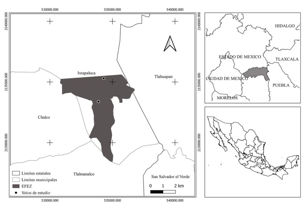
Figura 1. Localización del área de estudio Estación Forestal Experimental Zoquiapan (EFEZ).
En la región cercana a la zona de estudio se ubicaron 6 estaciones meteorológicas; sin embargo, los registros comprenden el periodo de 1961 al 2010, insuficientes para analizar el periodo de interés que se extiende hasta el 2023. Por tanto, se obtuvieron datos de precipitación y temperatura de la base de reanálisis NASA Prediction Of Worldwide Energy Resources (NASA POWER) (NASA POWER, 2023). Estos datos fueron sometidos a un análisis de correlación mediante el coeficiente de Pearson, con el propósito de compararlos con los registros de estaciones meteorológicas y confirmar la similitud y confiabilidad de la información proporcionada por NASA POWER (fig. 2). La vinculación de los eventos de sequía en el Estado de México con el índice de ancho de anillo total de P. montezumae se realizó con indicadores del Tzolkin Monitor de Sequía de Mesoamérica, desarrollado por el Instituto Mexicano de Tecnología del Agua (IMTA, 2020).
Para evaluar la influencia climática en el crecimiento radial de Pinus montezumae, se aplicó un análisis de función de respuesta, el cual consistió en obtener el coeficiente de correlación de Pearson, si los datos tienen una distribución normal en otro caso se obtuvo el coeficiente de Spearman entre las variables climáticas (precipitación total mensual, temperatura máxima, media y mínima) con los índices de las cronologías estandarizadas y residuales correspondientes al ancho de anillo total, madera temprana y madera tardía. Este análisis se hizo para el periodo 1982-2023 utilizando el coeficiente adecuado tras verificar la normalidad de los datos mediante la prueba de Shapiro-Wilk. Esto permitió determinar si el efecto de la variabilidad climática influye en el incremento radial del árbol.
Resultados
Se evaluó la relación entre la variabilidad climática y el crecimiento radial de Pinus montezumae en la Estación Forestal Experimental Zoquiapan. Para ello, se analizaron las correlaciones entre las cronologías estandarizadas y residuales del anillo total, madera temprana y tardía, con las variables climáticas de temperatura (promedio, máxima y mínima) y precipitación mensual. Los 26 árboles de Pinus montezumae presentaron diámetros que oscilaron entre 14 y 120 cm, y edades entre 34 y 123 años. De los 51 núcleos de crecimiento colectados, 45 (88%) fueron fechados con éxito; los restantes se excluyeron debido a la presencia de anillos falsos y ausentes.
Las cronologías del ancho de anillo total (AT), madera temprana (MTe) y madera tardía (MTa) abarcan un periodo común de 123 años, comprendido entre 1901 y 2023. La muestra más longeva data de 1901, mientras que la más reciente corresponde a 1981. El análisis de correlación entre las series de anillos de crecimiento, por segmentos de 50 años con traslapes de 25 años, indican que la calidad de fechado y la datación cruzada es correcta (p ˂ 0.01), superando la correlación mínima r = 0.3281 (tabla 1) establecida por Holmes (1983). Asimismo, los parámetros estadísticos de las series de anillos de crecimiento (tabla 1) respaldan el buen potencial dendroclimático de P. montezumae para estudios del crecimiento radial frente a la variabilidad climática.
Para identificar la función de respuesta del crecimiento radial a las variaciones climáticas, se generaron 2 cronologías: estándar y residual, a partir del índice de ancho de anillo total, madera temprana y madera tardía. Estas cronologías indican que el crecimiento promedio anual del ancho de anillo fue de 1.03 mm (tabla 2) y reflejan tendencias asociadas con periodos húmedos y de sequía. La cronología estándar fue la que determinó mejor la respuesta de P. montezumae a las fluctuaciones del clima, de acuerdo con la media del ancho de anillo (AT= 1.03, MTe = 1.0, MTa = 0.991), sensibilidad media (AT = 0.279, MTe = 0.138, MTa = 0.135), señal ruido (AT = 21.308, MTe = 15.353, MTa = 26.199). Las cronologías del índice de ancho de anillo total (IAA), madera temprana y madera tardía, tanto en su forma estándar (St) como residual (Rs), para P. montezumae comprenden un periodo de 123 años. Ambas series destacaron intervalos en los que el crecimiento radial fue superior a la media (fig. 3A), específicamente en los años 1901-1910, 1913-1917, 1942-1946, 1970-1972. En contraste, se observaron periodos de crecimiento por debajo del promedio durante 1923-1931, 1947-1950, 1961-1965, 1968-1976, 1998-2001 y 2021-2023.
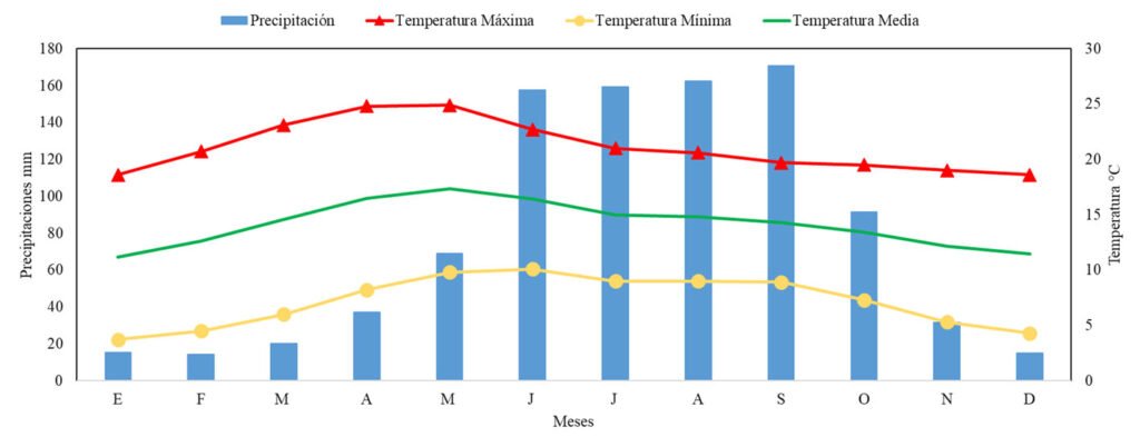
Figura 2. Climograma de la región EFEZ.
Las cronologías estándar y residual de la madera temprana presentaron una marcada variabilidad interanual en el crecimiento radial (fig. 3B). Los periodos con mayor desarrollo de madera temprana corresponden a los años 1901-1910, 1913-1916, 1931-1935, 1943-1947, 1978-1990 y 2002-2012. En contraste, se registró una menor formación de madera temprana durante los periodos 1923-1930, 1936-1942, 1961-1965, 1973-1977 y 1998-2001. Con respecto a las cronologías estándar y residual de la madera tardía también exhibieron una alta fluctuación interanual. Los periodos con mayor formación de madera tardía corresponden a los años 1903- 1904, 1907, 1909-1910, 1912, 1914-1915, 1917, 1923-1926, 1928-1930, 1935, 1937-1939, 1941- 1944, 1949-1951, 1954-1956, 1958-1962, 1969-1971, 1974-1977, 1983-1985, 1992 1995, 1996, 1998, 2003-2006, 2009-2010, 2014-2016 y 2018-2021 (fig. 3C).
Los eventos de sequía descritos por Domínguez (2016) y registrados en el Tzolkin Monitor de Sequía de Mesoamérica se asociaron a la cronología de ancho de anillo (fig. 4) y se observó que aquellos periodos de tiempo donde el crecimiento radial del árbol fue menor a la media anual corresponden a años con eventos de sequía, como son: la sequía de 1908 a 1910, las sequías de 1925, 1935, la de 1948 a 1954 que fue muy severa, 1957, 1960 a 1964, 1969, 1977. También se puede identificar que en el periodo de 1980 al 2023, el crecimiento radial estuvo influenciado por la presencia de sequías anuales de intensidad moderada, destacando el registro en la cronología de sequías severas en 2001, 2006-2012 y de 2018-2023.
Tabla 1
Estadísticos descriptivos de las series de anillos de crecimiento de P. montezumae.
| Parámetro estadístico | Anillo total | Madera temprana | Madera tardía |
| Intercorrelación entre series | 0.657 | 0.601 | 0.673 |
| Sensibilidad media | 0.281 | 0.324 | 0.278 |
| Desviación estándar | 0.875 | 0.758 | 0.223 |
| Autocorrelación de primer orden | 0.529 | 0.518 | 0.520 |
| Relación señal-ruido | 14.621 | 11.159 | 19.533 |
La función de respuesta del crecimiento radial de P. montezumae y la variabilidad del clima se analizó en el periodo común de 1981-2023. El análisis de correlación (coeficiente de Pearson), entre la cronología estandarizada de anillo total y la precipitación mensual, mostró correlaciones tanto positivas como negativas a lo largo del ciclo de crecimiento. La correlación entre el IAA estándar y precipitación mensual fue significativa en julio (r = 0.329, p = 0.033); mientras que, en el índice de madera temprana fue para septiembre del año anterior (r = -0.35, p = 0.049) y julio (r = 0.331, p = 0.032), para madera tardía fue en marzo (r = 0.373, p = 0.015) (fig. 5A). En los análisis de las cronologías residuales y la precipitación, la relación fue similar a la estándar, en el caso del índice de ancho de anillo fue significativa para septiembre del año anterior (r = -0.308, p = 0.046) y julio (r = 0.306, p = 0.048). Con respecto a la madera temprana, en septiembre del año anterior (r = -0.341, p = 0.027) y en madera tardía, en noviembre (r = 0.333, p = 0.031) y marzo (r = 0.373, p = 0.015) (fig. 5B).
La reciprocidad entre los índices de ancho de anillo AT, MTe, MTa y la temperatura (máxima, media y mínima) en el periodo común entre los años 1981 a 2023, reveló correlaciones negativas y positivas. Las asociaciones de los índices de ancho de anillo y la temperatura máxima, media y mínima con valores de coeficientes de correlación estadísticamente significativos (tabla 3), indican que las temperaturas máximas de septiembre y octubre del año anterior favorecieron el crecimiento del anillo total y la formación de madera temprana; sin embargo, en la cronología residual la temperatura máxima de enero afectó de forma negativa el desarrollo de madera tardía (fig. 6A, B).
Tabla 2
Estadísticas descriptivas de las cronologías estandarizada y residual de P. montezumae.
| Parámetros estadísticos | Cronologías | |||||
| Estándar | Residual | |||||
| Anillo total | Madera temprana | Madera tardía | Anillo total | Madera temprana | Madera tardía | |
| Ancho de anillo mm (media) | 1.03 | 1.00 | 0.991 | 0.992 | 0.987 | 0.991 |
| Sensibilidad media | 0.279 | 0.138 | 0.135 | 0.166 | 0.179 | 0.179 |
| Desviación estándar | 0.196 | 0.212 | 0.220 | 0.183 | 0.199 | 0.226 |
| Coeficiente de Gini | 0.110 | 0.120 | 0.124 | 0.104 | 0.113 | 0.124 |
| Autocorrelación de 1er orden | 0.125 | 0.092 | 0.196 | -0.162 | -0.180 | -0.100 |
| Relación señal-ruido | 21.308 | 15.353 | 26.199 | 27.802 | 20.144 | 34.543 |
| Señal expresada de la población (eps) | 0.950 | 0.934 | 0.958 | 0.965 | 0.953 | 0.972 |
Las correlaciones entre la temperatura mínima de octubre, noviembre, diciembre del año anterior con el índice de ancho de anillo de MTa y en diciembre con AT (fig. 6C, D), en la cronología estándar, fueron estadísticamente significativas; mientras que en la cronología residual solo fue significativa para noviembre; lo cual significa que las temperaturas mínimas de invierno favorecen la formación de madera tardía y puede deberse a que los árboles inician su etapa de letargo. Finalmente, la correlación entre la temperatura media de septiembre y octubre del año anterior fue estadísticamente significativa con el índice de madera tardía en la cronología estándar; en la cronología residual, únicamente la temperatura de octubre mostró una relación significativa (fig. 6E, F). Estos resultados reafirman la influencia de las temperaturas de otoño en la formación de madera tardía.
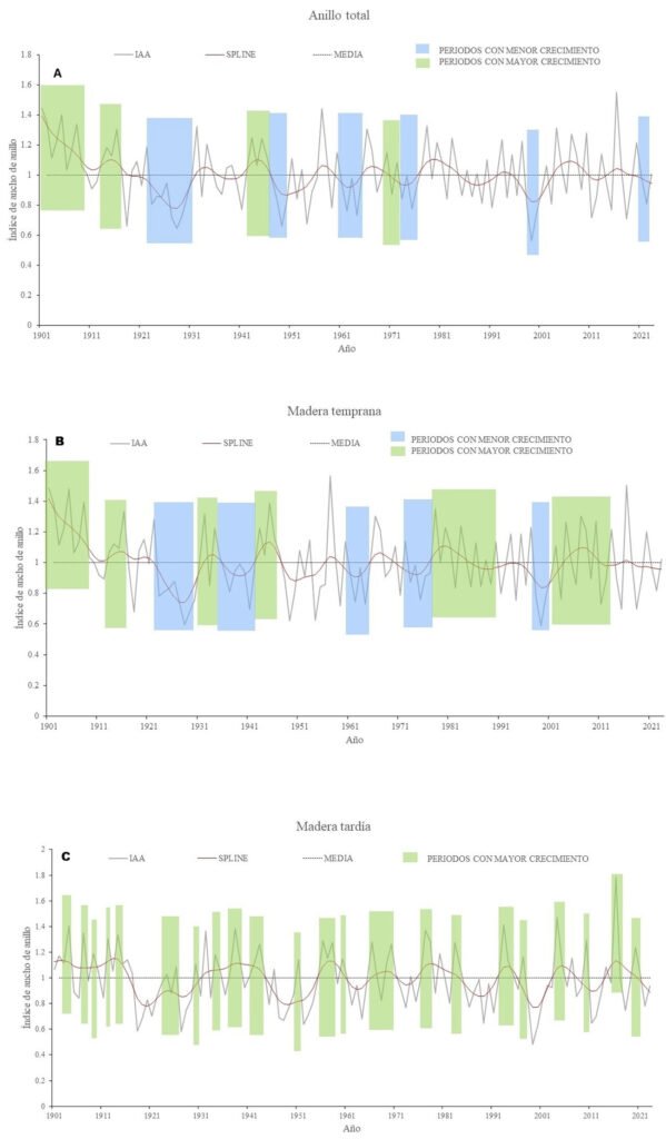
Figura 3. Cronología de índices de ancho de anillo de P. montezumae.
Discusión
Los resultados obtenidos aportan evidencia sobre la respuesta de Pinus montezumae a las condiciones ambientales, ya que se lograron identificar patrones de crecimiento mediante el fechado en 88% de las muestras. El porcentaje es considerado alto, puesto que en estudios dendrocronológicos es común excluir hasta 40% de las muestras debido a irregularidades en los anillos de crecimiento (Cerano-Paredes et al., 2014). La baja presencia de anillos falsos (menos de 5%) encontrada en P. montezumae coincide con lo registrado por Gutiérrez-García y Ricker (2019) y Villanueva-Díaz et al. (2016) para especies que habitan en la alta montaña.
Tabla 3
Coeficientes de correlación de Pearson de la relación entre índices de ancho de anillo y temperatura. * Mes del año anterior al inicio de la temporada de crecimiento.
| Temperatura | Mes | Índices de ancho de anillo de las Cronologías | |||||
| Estándar | Residual | ||||||
| Anillo total | Madera Temprana | Madera Tardía | Anillo total | Madera Temprana | Madera Tardía | ||
| Máxima | Septiembre* | r = 0.365 p = 0.017 | r = 0.353 p = 0.021 | – | r = 0.361 p = 0.018 | r = 0.356 p = 0.020 | – |
| Octubre* | r = 0.326 p = 0.034 | – | – | – | – | – | |
| Enero | – | – | – | – | – | r = -0.318 p = 0.039 | |
| Media | Septiembre* | – | – | r = 0.316 p = 0.041 | – | – | – |
| Octubre* | – | – | r = 0.362 p = 0.018 | – | – | r = 0.310 p = 0.045 | |
| Mínima | Octubre* | – | – | r = 0.323 p = 0.036 | – | – | – |
| Noviembre* | – | – | r = 0.365 p = 0.017 | – | – | r = 0.342 p = 0.026 | |
| Diciembre* | r = 0.318 p = 0.039 | – | r = 0.317 p = 0.040 | – | – | – |
Los valores de intercorrelación entre series fueron de 0.657 (anillo total), 0.601 (madera temprana) y 0.673 (madera tardía), similar a lo obtenido por Cortés-Cortés (2020) para P. montezumae en Coyuca de Catalán, Guerrero (r = 0.57), mayor al valor mínimo de 0 establecido por Holmes (1983), lo cual muestra que las intercorrelaciones de P. montezumae son estadísticamente significativas (p < 0.05). De acuerdo con Grissino-Mayer (2001), los valores de sensibilidad media del ancho total del anillo (0.281), madera temprana (0.324) y madera tardía (0.278) de P. montezumae representan una sensibilidad baja (0.135 – 0.179) e intermedia (0.279) en el ancho total del anillo. Estos valores son menores a los reportados para pináceas del norte de México, donde se obtuvieron valores mayores a 0.5 (Constante-García et al., 2010; Santillán-Hernández et al., 2016) y menores a los obtenidos para P. montezumae en Guerrero (0.31), según lo reportado por Cortés-Cortés (2020).
La autocorrelación de primer orden en los 3 índices de ancho de anillo muestra valores entre 0.092 y 0.196, lo cual es un criterio fundamental en estudios dendrocronológicos, debido a que una baja autocorrelación indica que el crecimiento radial no está significativamente influenciado por las condiciones climáticas del año anterior (Constante-García et al., 2010; Fritts, 1976). Estos resultados muestran que la especie es particularmente adecuada para estudios de reconstrucción climática porque permite registrar con mayor precisión las variaciones climáticas interanuales. De acuerdo con Briffa (1995), una cronología de sitio con un valor de señal expresada de la población (EPS) superior a 0.85, indica que el número de muestras es adecuado; en este estudio, se alcanzaron valores superiores, es decir, valores entre 0.934 y 0.972 para los 3 índices de crecimiento (AT, madera temprana y madera tardía), lo cual confirma la robustez de los datos analizados.
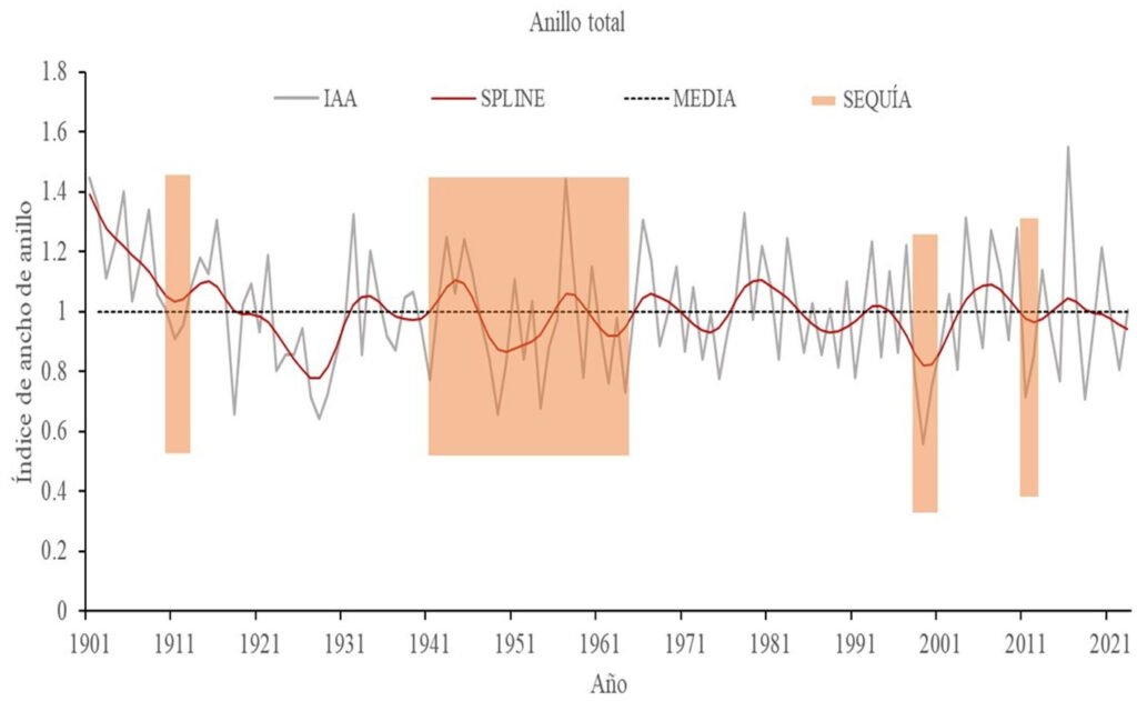
Figura 4. Vinculación de índice de ancho de anillo con eventos de sequía.
Los parámetros dendrocronológicos obtenidos para P. montezumae en este estudio, junto con los resultados reportados para la misma especie (Cortés-Cortés, 2020) y estudios de otras especies del centro del país, reconocidas por su buen potencial en este campo (Cerano-Paredes et al., 2014; Villanueva-Díaz et al., 2015, 2016), respaldan su utilidad en estudios dendrocronológicos. En consecuencia, se concluye que P. montezumae presenta un potencial dendrocronológico de moderado a alto, lo que la hace idónea para investigaciones orientadas a evaluar el impacto del clima y el cambio climático sobre el crecimiento radial. La relación entre el clima y el crecimiento radial indica que la disponibilidad de humedad, particularmente durante el invierno y la primavera, influye positivamente en el crecimiento de la especie. Este comportamiento coincide con un patrón que se presenta desde el sureste de los EUA hasta el centro de México, como lo han señalado diversos estudios (Allende et al., 2016; Cerano-Paredes et al., 2013; St. George et al., 2010; Villanueva-Díaz et al., 2016, 2017). Por lo tanto, las lluvias de baja intensidad, pero de larga duración junto con tasas moderadas de evaporación, permiten la retención de humedad en el suelo, favoreciendo el desarrollo durante los primeros meses de la temporada de crecimiento (Cerano-Paredes et al., 2009, 2011; Cleaveland et al., 2003; Constante-García et al., 2009; Díaz et al., 2002).
Por otra parte, las precipitaciones de verano y otoño del año de crecimiento actual presentan una variabilidad en su relación con las cronologías de P. montezumae; mientras que, los meses de otoño del año previo muestran correlaciones negativas y algunas estadísticamente significativas. Este patrón ha sido documentado también en investigaciones sobre otras especies del género Pinus (Cerano-Paredes et al., 2011, 2013; Chávez-Gándara et al., 2017; López-Hernández et al., 2018). Dicho comportamiento podría explicarse por la abundancia de lluvia durante estos periodos, que supera la capacidad de infiltración del suelo, provoca saturación de sus partículas, genera escurrimientos superficiales y limita así su disponibilidad para el desarrollo del árbol, así como por el hecho de que la mayor parte de los fotosintatos producidos en la temporada de lluvias se asignan al desarrollo de la copa, y se deja en segundo plano el incremento en el diámetro del tronco (Fritts, 1976). No obstante, esta lluvia es de gran importancia, pues parte de ella se almacena en el suelo y puede ser utilizada en la siguiente etapa de crecimiento (Meko et al., 1995).
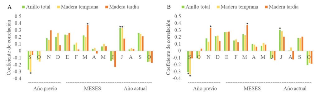
Figura 5. Coeficientes de correlación de precipitación e índices de ancho de anillo: A, estándar; B, residual.
El crecimiento de P. montezumae está principalmente influenciado y regulado por la disponibilidad de humedad durante el otoño del año previo y la primavera del año en curso. Al igual que otras especies estudiadas en investigaciones dendrocronológicas en el norte y centro de México, P. montezumae mostró una respuesta significativamente mayor a la precipitación que a la temperatura (Cerano-Paredes et al., 2013; Constante-García et al., 2010; Villanueva-Díaz et al., 2015, 2017). Los análisis de la temperatura máxima, mínima y media han identificado relaciones positivas entre estos factores y el crecimiento radial de los árboles en diversas partes del mundo, demostrando que la temperatura es un factor determinante en el desarrollo de los bosques, reflejándose en procesos clave, como la reactivación del cambium vascular, la diferenciación celular del xilema y la fotosíntesis, basándose en análisis de índices de ancho de anillo (Antonucci et al., 2017; Li et al., 2017, 2018; Zhu et al., 2016). Este estudio confirma la importancia de la temperatura en el crecimiento del P. montezumae debido a que se logra evidenciar, en algunos meses, el impacto de esta variable. De manera similar a lo observado en el estudio de P. montezumae realizado por Cortés-Cortés (2020), se identificaron principalmente relaciones positivas entre la temperatura máxima y la cronología estandarizada; además, en ambos estudios se observó una disminución en los valores estadísticamente significativos al correlacionarse con la cronología residual.
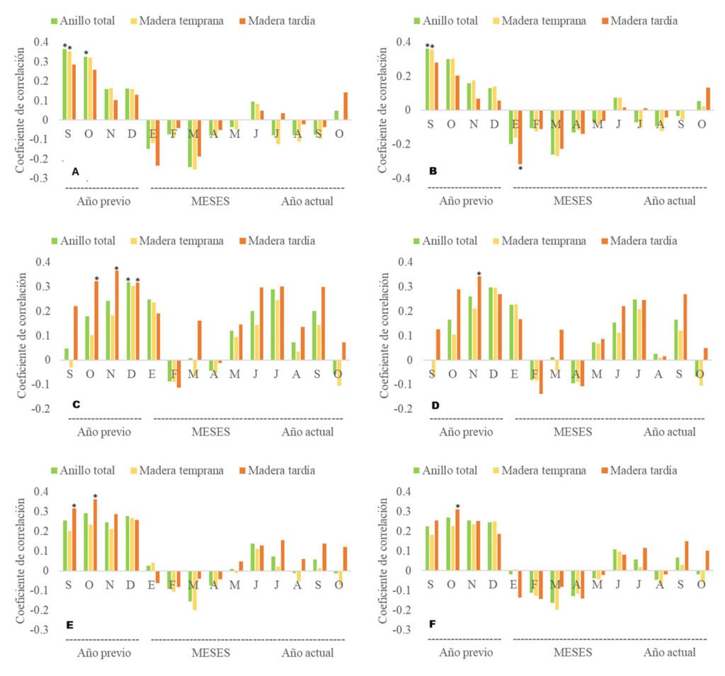
Figura 6. Coeficientes de correlación de temperatura e índices de ancho de anillo: A, relación temperatura máxima-cronología estándar; B, relación temperatura máxima-cronología residual; C, relación temperatura mínima – cronología estándar; D, relación temperatura mínima-cronología residual; E, relación temperatura media-cronología estándar; F, relación temperatura media-cronología residual.
En otros estudios de dendrocronología como el de Pinus hartwegii en el monte Tláloc ubicado también en la Faja Volcánica Transmexicana (Astudillo-Sánchez et al., 2017, 2019) y de Pinus oocarpa Schiede ex Schltdl del ejido Ojo de Agua, La Independencia en Chiapas, se han identificado correlaciones positivas entre las cronologías de ancho de anillo total y la temperatura máxima, éstas sugieren que la temperatura máxima incide en el crecimiento y desarrollo de madera tardía, tanto en la región central del país como en el sur, aunque se trate de especies con diferente rango de distribución (Astudillo-Sánchez et al., 2017, 2019; López-Hernández et al., 2018). La temperatura mínima mostró una influencia positiva en la mayoría de los meses analizados y destacó su efecto sobre la cronología de madera tardía, la cual presentó el mayor número de correlaciones positivas estadísticamente significativas. Estos hallazgos son consistentes con lo reportado en otros estudios dendrocronológicos realizados en México, que han encontrado correlaciones positivas significativas entre las temperaturas invernales y el crecimiento de diversas coníferas (Cerano-Paredes et al., 2012, 2014; Correa-Díaz et al., 2019; Chávez-Gándara et al., 2017; Huante et al., 1991; López-Hernández et al., 2018).
El crecimiento de las especies en respuesta a las temperaturas mínimas se debe, en gran medida, a que estas condiciones favorecen una menor evaporación del suelo y las plantas tienen una mayor disponibilidad de agua para el crecimiento (Cerano-Paredes et al., 2011; Chávez-Gándara et al., 2017). Con relación a la temperatura media, diversos estudios reportan que esta influye de manera negativa en el crecimiento radial (Cortés-Cortés et al., 2020; Manzanilla-Quiñones et al., 2020; Villanueva-Díaz et al., 2016). Sin embargo, en la presente investigación se identificó la presencia de correlaciones positivas, coincidiendo con lo reportado para otras especies de coníferas (Cerano-Paredes et al., 2014; Correa-Díaz et al., 2019). En la cronología residual se observaron correlaciones negativas de enero y mayo, un patrón que también se presentó al correlacionarse con la temperatura máxima. Este comportamiento puede atribuirse tanto al déficit hídrico como a que las temperaturas en la zona de estudio, en ciertos meses, se sitúan fuera del rango óptimo para la fotosíntesis en algunas coníferas, el cual oscila entre 15 y 25 °C, reduciéndose gradualmente en ambos extremos (Huxman et al., 2003; McCullough et al., 2017; Williams et al., 2013).
El crecimiento radial de P. montezumae responde a una interacción entre la temperatura y la precipitación. La disponibilidad de humedad en meses clave, como julio y marzo, junto con las temperaturas máximas en septiembre y octubre del año anterior, regulan conjuntamente la formación del crecimiento anual. Esto sugiere que el aumento en la temperatura puede favorecer el crecimiento solo cuando la precipitación es suficiente para mantener los procesos fisiológicos del árbol. Asimismo, las temperaturas mínimas durante el invierno parecen favorecer la formación de la madera tardía, lo que resalta la importancia de las condiciones térmicas en diferentes fases del ciclo anual. Los resultados coinciden con lo reportado por Harvey et al. (2020), quienes documentaron que el crecimiento radial en bosques templados está influenciado positivamente por inviernos cálidos, pero el efecto favorable del aumento temperatura puede verse limitado si no existe suficiente precipitación durante el verano. Por lo tanto, el impacto del cambio climático en el crecimiento de P. montezumae dependerá de la variación simultánea de la precipitación y la temperatura, por lo que es importante considerar ambas variables para predecir la respuesta de la especie en escenarios futuros.
Agradecimientos
A la Secretaría de Ciencia, Humanidades, Tecnología e Innovación (Secihti) por el otorgamiento de una beca para estudios de maestría al primer autor. A la División de Ciencias Forestales de la Universidad Autónoma Chapingo y al personal responsable de la Estación Forestal Experimental Zoquiapan, por el acceso y apoyo para la realización de esta investigación.
Referencias
Aber, J., Neilson, R. P., McNulty, S., Lenihan, J. M., Bachelet, D. y Drapek, R. J. (2001). Forest processes and global environmental change: predicting the effects of individual and multiple stressors. BioScience, 51, 735. https://doi.org/10.1641/0006-3568(2001)051
Allende, T. C., Mendoza, M. E., Pérez-Salicrup, D. R., Villanueva-Díaz, J. y Lara, A. (2016). Climatic responses of Pinus pseudostrobus and Abies religiosa in the Monarch Butterfly Biosphere Reserve, Central Mexico. Dendrochronologia, 38, 103–116. https://doi.org/10.1016/j.dendro.2016.04.002
Antonucci, S., Rossi, S., Deslauriers, A., Morin, H., Lombardi, F., Marchetti, M. et al. (2017). Large scale estimation of xylem phenology in black spruce through remote sensing. Agricultural and Forest Meteorology, 233, 92–100. https://doi.org/10.1016/j.agrformet.2016.11.011
Astudillo-Sánchez, C. C., Fowler, M. S., Villanueva-Díaz, J., Endara-Agramont, A. R. y Soria-Díaz, L. (2019). Recruitment and facilitation in Pinus hartwegii, a Mexican alpine treeline ecotone, with potential responses to climate warming. Trees, 33, 1087–1100. https://doi.org/10.1007/s00468-019-01844-3
Astudillo-Sánchez, C. C., Villanueva-Díaz, J., Endara-Agramont, A. R., Nava-Bernal, G. E. y Gómez-Albores, M. A. (2017). Climatic variability at the treeline of Monte Tlaloc, Mexico: a dendrochronological approach. Trees, 31, 441–453. https://doi.org/10.1007/s00468-016-1460-z
Benito, F. G. (2014). Archivos climáticos y paleohidrológicos. Introducción a datos proxy y su análisis. Madrid: CSIC- Museo Nacional de Ciencias Naturales.
Briffa, K. R. (1995). Interpreting high-resolution proxy climate data. The example of dendroclimatology. En H. von Storch y A. Navarra (Eds.), Analysis of climate variability, applications of statistical techniques (pp. 77–94). Berlin, Heidelberg: Springer. https://doi.org/10.1007/978-3-662-03167-4_5
Bunn, A. G. (2010). Statistical and visual crossdating in R using the dplR library. Dendrochronologia, 28, 251–258. https://doi.org/10.1016/j.dendro.2009.12.001
Bunn, A.G. (2008). A dendrochronology program library in R (dplR). Dendrochronologia, 26, 115–124. https://doi.org/10.1016/j.dendro.2008.01.002
Cassman, K. G. y Wood, S. (2005) Cultivated systems. En R. Hassan, R. Scholes y N. Ash (Eds.), Ecosystems and human well-being: current state and trends (pp. 745–794). Washington, DC; Millennium Ecosystem Assessment – Island Press.
Cerano-Paredes, J., Villanueva-Díaz J., Cervantes-Martínez, R., Vázquez-Selem, L., Trucios-Caciano, R. y Guerra-de la Cruz, V. (2014). Reconstrucción de precipitación invierno-primavera para el Parque Nacional Pico de Tancítaro, Michoacán. Investigaciones Geográficas, 83, 41–54. https://doi.org/10.14350/rig.35190
Cerano-Paredes, J., Villanueva-Díaz, J., Fulé, P. Z., Arreola-Ávila, J. G., Sánchez-Cohen, I. y Valdez-Cepeda, R. D. (2009). Reconstrucción de 350 años de precipitación para el suroeste de Chihuahua, México. Madera y Bosques, 15, 27–44. https://doi.org/10.21829/myb.2009.1521189
Cerano-Paredes, J., Villanueva-Díaz, J., Valdez-Cepeda, R. D., Méndez-González, J. y Constante-García, V. (2011). Sequías reconstruidas en los últimos 600 años para el noreste de México. Revista Mexicana de Ciencias Agrícolas, 2, 235–249. https://doi.org/10.21829/myb.2009.1521189
Cerano-Paredes, J., Rivera-González, M., Estrada-Ávalos, J., Trucios-Caciano, R. y Ríos-Saucedo, J. C. (2012). Análisis dendrocronológico de Pinus cooperi en Durango, México. Agrofaz, 12, 81–88.
Cerano-Paredes, J., Villanueva-Díaz, J., Cervantes-Martínez, R., Trucios-Caciano, R. y Guerrero-Soto, J. L. (2013). Reconstrucción de sequías fuertes en el Parque Nacional “Pico de Tancítaro”, Michoacán. Revista Chapingo, Serie Zonas Áridas, 2, 57–62. https://doi.org/10.5154/r.rchsza.2012.06.026
Chávez-Gándara, M. P., Cerano-Paredes, J., Nájera-Luna, J. A., Pereda-Breceda, V., Esquivel-Arriaga, G., Cervantes-Martínez, R. et al. (2017). Reconstrucción de la precipitación invierno-primavera con base en anillos de crecimiento de árboles para la región de San Dimas, Durango, México. Bosque, 38, 387–399. https://dx.doi.org/10.4067/S0717-92002017000200016
Cleaveland, M. K., Stahle, D. W., Therrell, M. D., Villanueva-Díaz, J. y Burns, B. T. (2003). Tree-ring reconstructed winter precipitation and tropical teleconnections in Durango, Mexico. Climatic Change, 59, 369–388. https://doi.org/10.1023/A:1024835630188
Conanp (Comisión Nacional de Áreas Naturales Protegidas). (2013). Programa de manejo del Parque Nacional Iztaccíhuatl-Popocatépetl. México. Recuperado el 15 agosto, 2024 de: https://conanp.gob.mx/conanp/dominios/iztapopo/documentos/programa_demanejo_izta_popo.pdf
Constante-García, V., Villanueva-Díaz, J., Cerano-Paredes, J., Cornejo-Oviedo, E. H. y Valencia-Manzo, S. (2009). Dendrocronología de Pinus cembroides Zucc. y reconstrucción de precipitación estacional para el Sureste de Coahuila. Ciencia Forestal en México, 34, 17–39.
Constante-García, V., Villanueva-Díaz, J., Cerano-Paredes, J. y Estrada-Ávalos, J. (2010). Parámetros para definir el potencial dendrocronológico. Folleto técnico número 19. Gómez Palacio, Durango: Instituto Nacional de Investigaciones Forestales, Agrícolas y Pecuarias.
Cook, E. R. y Kairiukstis, L. A. (1990) Methods of dendrochronology. Applications in the environmental sciences. Dordrecht, Holanda: International Institute for Applied Systems Analysis. Kluwer Academic Publishers.
Correa-Díaz, A., Silva, L. C. R., Horwath, W. R., Gómez-Guerrero, A., Vargas-Hernández, J., Villanueva-Díaz, J. et al. (2019). Linking remote sensing and dendrochronology to quantify climate-induced shifts in high-elevation forests over space and time. Journal of Geophysical Research: Biogeosciences, 124, 166–183. https://doi.org/10.1029/2018JG004687
Cortés-Cortés, O., Cornejo-Oviedo, E. H., Cerano-Paredes, J., Cervantes-Martínez, R., Flores-López, C. y Valencia-Manzo, S. (2020). Relationship between climate variability and radial growth of Pinus montezumae Lamb. in Coyuca de Catalán, Guerrero. Revista Chapingo, Serie Ciencias Forestales y del Ambiente, 27, 109–126. https://doi.org/10.5154/r.rchscfa.2020.03.012
Díaz, S. C., Therrell, M. D., Stahle, D. W. y Cleaveland, M. K. (2002). Chihuahua (México) winter-spring precipitation reconstructed from tree rings, 1647-1992. Climate Research, 22, 237–244. https://doi.org/10.3354/cr022237
Domínguez, J. (2016). Revisión histórica de las sequías en México: de la explicación divina a la incorporación de la ciencia. Tecnología y Ciencias del Agua, 7, 77–93.
Farjon, A., Pérez-de la Rosa, J. A. y Styles, B. T. (1997). Guía de campo de los pinos de México y América Central. Oxford, UK: The Royal Botanic Gardens, Kew/ Instituto Forestal de Oxford, Universidad de Oxford.
Fritts, H. C. (1976). Tree rings and climate. New York: Academic Press Inc.
Grissino-Mayer, H. D. (2001). Evaluating crossdating accuracy: a manual and tutorial for the computer program COFECHA. Tree-Ring Research, 57, 205–221.
Gutiérrez-García, G. y Ricker, M. (2019). Influencia del clima en el crecimiento radial en cuatro especies de coníferas en la sierra de San Antonio Peña Nevada (Nuevo León, México). Revista Mexicana de Biodiversidad, 90, e902676. https://doi.org/10.22201/ib.20078706e.2019.90.2676
Harvey, J. E., Smiljanić, M., Scharnweber, T., Buras, A., Cedro, A. Cruz-García, R. et al. (2020). Tree growth influenced by warming winter climate and summer moisture availability in northern temperate forests. Global Change Biology, 26, 2505–2518. https://doi.org/10.1111/gcb.14966
Holmes, R. L. (1983). Computer-assisted quality control in tree-ring dating and measurement. Tree-Ring Bulletin, 43, 69–78.
Howard, I. M., Stahle D. W., Torbenson, M. C. A. y Griffin, D. (2021). The summer precipitation response of latewood tree-ring chronologies in the southwestern United States. International Journal of Climatology, 41, 2913–2933. https://doi.org/10.1002/joc.6997
Huante, P., Rincón, E. y Swetnam, T. W. (1991). Dendrochronology of Abies religiosa in Michoacán, Mexico. Tree-Ring Bulletin, 51, 15–28.
Huxman, T. E., Turnipseed, A. A., Sparks, J. P., Harley, P. C. y Monson, R. K. (2003). Temperature as a control over ecosystem CO2 fluxes in a high-elevation, subalpine forest. Oecologia, 134, 537–546. https://doi.org/10.1007/s00442-002-1131-1
IMTA (Instituto Mexicano de la Tecnología del Agua). (2020). Tzolkin Monitor de Sequía de Mesoamérica. Instituto Mexicano de la Tecnología del Agua, Secretaría de Medio Ambiente Recursos Naturales, México. Recuperado el 18 agosto, 2024 de: http://galileo.imta.mx/Sequias/moseq/index.html
IPCC (Intergovernmental Panel on Climate Change). (2014). Climate Change 2014. Synthesis report. Contribution of working groups I, II and III to the fifth assessment report of the Intergovernmental Panel on Climate Change. Génova, Suiza: IPCC. Disponible: https://archive.ipcc.ch/pdf/assessment-report/ar5/syr/SYR_AR5_FINAL_full_wcover.pdf
IPCC (Intergovernmental Panel on Climate Change). (2021). Climate change 2021. A summary for all. IPCC. Disponible: https://www.ipcc.ch/report/ar6/wg1/downloads/outreach/IPCC_AR6_WGI_SummaryForAll.pdf
Li, M., Duan, J., Wang, L. y Zhu, H. (2018). Late summer temperature reconstruction based on tree-ring density for Sygera Mountain, southeastern Tibetan Plateau. Global and Planetary Change, 163, 10–17. https://doi.org/10.1016/j.gloplacha.2018.02.005
Li, X., Liang, E., Gricar, J., Rossi, S., Čufar, K. y Ellison, A. M. (2017). Critical minimum temperature limits xylogenesis and maintains treelines on the southeastern Tibetan Plateau. Science Bulletin, 62, 804–812. https://doi.org/10.1016/).scib.2017.04.025
López-Hernández, M. I., Cerano-Paredes, J., Valencia-Manzo, S., Cornejo-Oviedo, E. H., Villanueva-Díaz, J., Cervantes-Martínez, R. et al. (2018). Respuesta del crecimiento de Pinus oocarpa a variables climáticas en Chiapas, México. Biología Tropical, 66, 1580–1596. http://dx.doi.org/10.15517/rbt.v66i4.32663
Manzanilla-Quiñones, U., Aguirre-Calderón, O. A., Jiménez-Pérez, J. y Villanueva-Díaz, J. (2020). Sensibilidad climática en anchuras de anillos de crecimiento de Pinus hartwegii: una especie alpina mexicana con potencial dendroclimático. Revista Mexicana de Biodiversidad, 91, e913117. https://doi.org/10.22201/ib.20078706e.2020.91.3117
McCullough, I. M., Davis, F. W. y Williams, A. P. (2017). A range of possibilities: assessing geographic variation in climate sensitivity of ponderosa pine using tree rings. Forest Ecology and Management, 402, 223–233. https://doi.org/10.1016/j.foreco.2017.07.025
Meko, D., Stockton, C. W. y Boggess, W. R. (1995). The tree-ring record of severe sustained drought. JAWRA Journal of the American Water Resources Association, 31, 789–801. https://doi.org/10.1111/j.1752-1688.1995.tb03401.x
Meko, D. M. y Baisan, C. H. (2001). Pilot study of latewood-width of conifers as an indicator of variability of summer rainfall in the North American monsoon region. International Journal of Climatology, 21, 697–708. https://doi.org/10.1002/joc.646
NASA POWER. (2023). Prediction Of Worldwide Energy Resources. National Aeronautics and Space Administration (NASA), Washington D. C. Recuperado el 31 junio, 2024 de: https://power.larc.nasa.gov
Osorio-Osorio, J. A., Astudillo-Sánchez, C. C., Villanueva-Díaz, J., Soria-Díaz, L. y Vargas-Tristán, V. (2020). Reconstrucción histórica de la precipitación en la Reserva de la Biosfera El Cielo, México, mediante anillos de crecimiento en Taxodium mucronatum (Cupressaceae). Revista de Biología Tropical, 8, 818–832. https://doi.org/10.15517/rbt.v68i3.39624
Posit team (2024). RStudio. Integrated development environment for R. Posit Software, PBC, Boston, MA. https://www.posit.co/
Rzedowski, J. (2006). Vegetación de México. Comisión Nacional para el Conocimiento y Uso de la Biodiversidad. http://www.conabio.gob.mx/institucion/centrodoc/doctos/librosdigitales/VegetaciondeMexico/Portadaypaglegales.pdf
Santillán-Hernández, M., Cornejo-Oviedo, E. H., Villanueva-Díaz, J., Cerano-Paredes, J., Valencia-Manzo, S. y Capó-Arteaga, M. Á. (2016). Potencial dendroclimático de Pinus pinceana Gordon en la Sierra Madre Oriental. Madera y Bosques, 16, 17–30. https://doi.org/10.21829/myb.2010.1611177
Schweingruber, F. H. (1988). Tree rings: basics and applications of dendrochronology. Holanda: Dordrecht, Holanda: Kluwer Academic Publishers Group.
St. George, S., Meko, D. M. y Cook, E. R. (2010). The seasonality of precipitation signals embedded within the North American Drought Atlas. The Holocene, 20, 983–988. https://doi.org/10.1177/0959683610365937
Stokes, M. A. y Smiley, T. L. (1996). An introduction to tree-ring dating. Tucson: The University of Arizona Press.
Vaganov, E. A., Hughes, M. K. y Shashkin, A. V. (2006). Growth dynamics of conifer tree rings: images of past and future environments. Berlín, Heidelberg: Springer-Verlag.
Villanueva-Díaz, J., Rubio-Camacho, E. A., Chávez-Durán, A. A., Zavala-Aguirre, J. L., Cerano-Paredes, J. y Martínez-Sifuentes, A. R. (2017). Respuesta climática de Pinus oocarpa Schiede Ex Schetol en el Bosque La Primavera, Jalisco. Madera y Bosques, 24, 1–14. https://doi.org/10.21829/myb.2018.2411464
Villanueva-Díaz, J., Cerano-Paredes, J., Vázquez-Selem, L., Stahle, D. W., Fulé, P. Z., Yocom, L. L. et al. (2015). Red dendrocronológica del pino de altura (Pinus hartwegii Lindl.) para estudios dendroclimáticos en el noreste y centro de México. Investigaciones Geográficas, 86, 5–14. https://doi.org/10.14350/rig.42003
Villanueva-Díaz, J., Vázquez-Selem, L., Gómez-Guerrero, A., Cerano-Paredes, J., Aguirre-González, N. A. y Franco-Ramos, O. (2016). Potencial dendrocronológico de Juniperus monticola Martínez en el Monte Tláloc, México. Revista Fitotecnia Mexicana, 39, 175–185. https://doi.org/10.35196/rfm.2016.2.175-185
Williams, A. P., Allen, C. D., Macalady, A. K., Griffin, D., Woodhouse, C. A., Meko, D. M. et al. (2013). Temperature as a potent driver of regional forest drought stress and tree mortality. Nature Climate Change, 3, 292–297. https://doi.org/10.1038/nclimate1693
Zhu, L., Zhang, Y., Li. Z., Guo, B. y Wang, X. (2016). A 368-year maximum temperature reconstruction based on tree-ring data in the northwestern Sichuan Plateau (NWSP), China. Climate of the Past, 12, 1485–1498. https://doi.org/10.5194/cp-12-1485-2016

Population density and sexual maturity of Ambystoma lermaense, an endangered species in central Mexico
Densidad poblacional y madurez sexual de Ambystoma lermaense, una especie amenazada en el centro de México
Gerardo Legorreta-Balbuena a, Carlos Omar Becerra-Soria b, Susana Hernández-Monasterio b, Gabriela Parra-Olea b, *
a Universidad Nacional Autónoma de México, Instituto de Investigaciones Biomédicas, Laboratorio de Biología Integrativa, Tercer Circuito s/n, Ciudad Universitaria, Col. Copilco Universidad, 04510 Ciudad de México, Mexico
b Universidad Nacional Autónoma de México, Instituto de Biología, Departamento de Zoología, Tercer Circuito s/n, Ciudad Universitaria, Col. Copilco Universidad, 04510 Ciudad de México, Mexico
*Corresponding author: gparra@ib.unam.mx (G. Parra-Olea)
Received: 21 January 2025; accepted: 14 November 2025
Abstract
Ambystoma lermaense, an endangered salamander species endemic to central Mexico, faces significant threats from habitat degradation, pollution, and human activities. This study evaluates the population density, structure, and sexual maturity of A. lermaense in Capilla Vieja, Estado de México, over 3 time periods: 2009, 2010, and 2020. Using visual encounter surveys along a 730-m stream transect, we recorded population densities of 0.021 individuals/m² in 2009, 0.070 individuals/m² in 2010, and 0.075 individuals/m² in 2020, reflecting relative stability despite anthropogenic pressures. Juveniles accounted for 87% of the population, with sexual maturity observed at a snout-vent length of 60 mm, supported by histological evidence of vitellogenic oocytes in females and mature sperm in males. Our study provides important insights into the population dynamics and sexual maturity of A. lermaense in the sampling locality, where this species had not been previously studied.
Keywords: Ambystomatidae; Population structure; Paedomorphosis; Vitellogenic oocytes; Mature sperm; Decline
Resumen
Ambystoma lermaense, una especie de salamandra en peligro de extinción endémica del centro de México, enfrenta amenazas significativas debido a la degradación del hábitat, la contaminación y las actividades humanas. Este estudio evalúa la densidad poblacional, estructura y madurez sexual de A. lermaense en Capilla Vieja, Estado de México, durante 3 períodos: 2009, 2010 y 2020. Utilizando muestreos visuales a lo largo de un transecto de 730 m en un arroyo, registramos densidades poblacionales de 0.021 individuos/m² en 2009, 0.070 individuos/m² en 2010 y 0.075 individuos/m² en 2020, lo cual refleja una estabilidad relativa a pesar de las presiones antropogénicas. Los juveniles representaron 87% de la población y se observó madurez sexual a un tamaño de 60 mm de longitud hocico-cloaca, sustentado por evidencia histológica de ovocitos vitelogénicos en hembras y espermatozoides maduros en machos. Nuestro estudio proporciona información importante sobre la dinámica poblacional y la madurez sexual de A. lermaense en la localidad de muestreo, donde esta especie no había sido estudiada previamente.
Palabras clave: Ambystomatidae; Estructura poblacional; Paedomorfosis; Ovocitos vitelogénicos; Espermatozoides maduros; Declive
Introduction
Amphibians worldwide are experiencing unprecedented declines, driven by a combination of habitat loss, pollution, climate change, invasive species, and disease (Grant et al., 2016; Stuart et al., 2004). These declines are particularly concerning for high-altitude amphibians, which often have restricted ranges and specialized habitat requirements (Green, 2003; Pounds, 2001; Stuart et al., 2004). As indicators of ecosystem health, amphibians play critical roles in maintaining ecological balance, yet they are disproportionately affected by anthropogenic pressures (Blaustein & Wake, 1990). Among these, Ambystoma lermaense, an endangered salamander species endemic to central Mexico, exemplifies the challenges faced by amphibians in fragmented and degraded habitats (IUCN SSC Amphibian Specialist Group, 2015).
Ambystoma lermaense, inhabits high-altitude streams at elevations ranging from 2,500 to 3,000 m asl (IUCN SSC Amphibian Specialist Group, 2015). This facultatively paedomorphic species is found in aquatic habitats such as lakes, ponds, marshes, and occasionally streams (Everson et al., 2021; IUCN SSC Amphibian Specialist Group, 2015), which are increasingly impacted by human activities (Reilly & Brandon, 1994). Agricultural expansion, livestock grazing, pollution, and urban development threaten the quality and connectivity of these aquatic habitats (Egea-Serrano et al., 2012; Robles-Mendoza et al., 2009). These pressures, combined with seasonal hydrological fluctuations and climate variability, pose significant risks to the long-term viability of A. lermaense populations (Dirzo et al., 2022; Huacuz-Elías, 2003).
Understanding population dynamics is a cornerstone of effective conservation planning. Accurate data on population density, structure, and trends are essential for identifying populations at risk and prioritizing interventions (Pechmann et al., 1991). Previous studies on species of the genus Ambystoma have revealed a wide spectrum of population densities, ranging from critically low levels in urbanized environments to exceptionally high densities in protected areas. For instance, the Mexican axolotl (A. mexicanum) exhibits densities as low as 0.001 individuals per square meter in the urban canals of Xochimilco (Contreras et al., 2009), while A. rivulare densities reach 2.3 individuals per square meter in the protected natural area Reserva de la Biósfera Mariposa Monarca (Huacuz-Elías, 2003). These disparities underscore the profound impact of habitat quality and protection on amphibian populations.
Despite its resilience in suboptimal conditions, A. lermaense remains highly vulnerable to habitat degradation and fragmentation (Jacinto-Maldonado et al., 2023). In the Capilla Vieja region of Estado de México, semi-intensive livestock activities and seasonal stream drying compound the challenges faced by this species (previously recognized in this locality as A. granulosum; Everson et al., 2021). As part of a natural protected area, Capilla Vieja offers a unique opportunity to study how A. lermaense populations persist in a landscape that combines elements of protection and human impact. The site’s connectivity to a broader watercourse system also provides insights into the role of habitat corridors in sustaining population viability.
This study examines the population density, structure, and sexual maturity of A. lermaense in Capilla Vieja over 3 time periods: 2009, 2010, and 2020. By situating these findings within the broader context of Ambystoma conservation, we aim to draw comparisons with other populations and species to better understand the factors driving population trends. The research also highlights the critical role of protected areas and localized conservation actions in addressing the multifaceted threats to amphibians. This work contributes to the growing body of knowledge needed to inform strategies for safeguarding A. lermaense and other endangered amphibians in Mexico’s diverse ecosystems.
Materials and methods
The study was conducted in a section of a stream located in Capilla Vieja, municipality of Amanalco de Becerra, Estado de México, at coordinates 19º13’22” N, 99º59’12” W, with an elevation ranging from 2,790 to 2,870 m asl (Fig. 1). The predominant vegetation in this area is pine-oak-fir forest. The climate is temperate subhumid, with summer rains, an average annual temperature of 12 °C, and temperature extremes ranging from 0.5 °C to 29.7 °C (Rentería et al., 2005). Capilla Vieja is part of the sustainable ecosystem management subzone for agricultural areas within the Natural Protected Area known as Área de Protección de Recursos Naturales de las Cuencas de los Ríos Valle de Bravo, Malacatepec, Tilostoc y Temascaltepec (Semarnat, 2018).
The study stream crosses an extensive grassland plain that is used for semi-intensive livestock activities, including sheep, cattle, and horses. The stream during the rainy season features shallow areas with nearly stagnant water. In certain sections, the bottom is extremely soft, with mud depths ranging from 15 to 25 cm and exceeding 50 cm in some points. The stream width varies between 2 and 5 m, expanding during the rainy season and shrinking or disappearing during the dry season. This stream is part of a connected watercourse system that flows in a northeast-southwest direction, contributing to the water supply of the Capilla Vieja lagoon (Comisión Nacional de Áreas Naturales Protegidas, 2018).
Samplings were conducted once a month from July to October during 3 periods corresponding to the years 2009, 2010 and 2020. Each month, a 730 m transect with a width of 3 m along the stream was surveyed (starting coordinates: 19°13’10.81” N, 99°59’4.95” W; ending coordinates: 19°13’3.73” N, 99°59’15.13” W). Sampling was carried out using the visual encounter survey method between 09:00 and 14:00 hours (Heyer et al., 1994; Lips et al., 1999), recording the total number of individuals. Each individual was captured using hand nets and placed in 20-liter plastic containers filled with water from the stream.
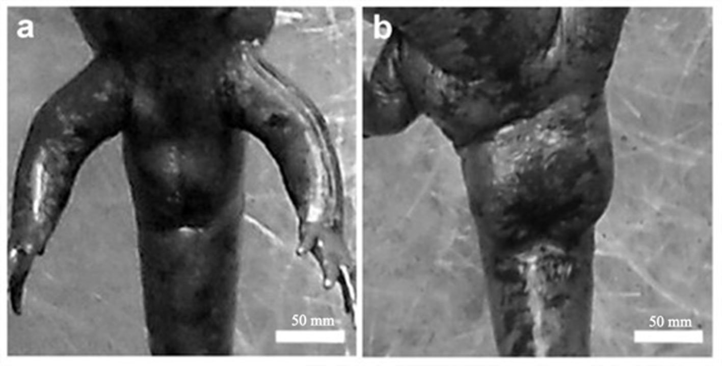
Morphometric measurements were recorded for each specimen: snout-vent length (SVL), total length (TL), and weight (W). Individuals were classified into 2 categories: adult metamorphic (males and females) and larvae (juveniles), a category that included individuals with gills for whose sex could not be determined. Population density was calculated by dividing the total number of individuals (N) by the sampled area of the stream (N/m²) (Williams et al., 2002), and it was estimated for each sampling period. Males and females were identified based on the size and shape of the cloaca (Aguilar-Miguel et al., 2009; Taylor, 1940). In females, the cloaca is flat and smaller (Fig. 2a), whereas in males it is enlarged due to high glandular activity (Fig. 2b).
To estimate the size at sexual maturity, a sample of 52 individuals was collected from random points along the stream during the 2009 and 2010 sampling periods. The sample included individuals ranging in size from 50 to 115 mm in SVL. An ANOVA was used to assess the relationship between body size and sexual maturity.
To euthanize the specimens, they were anesthetized using a 0.1% solution of MS-222 (tricaine methanesulfonate) for 20 min (Mitchell, 2009; Rubio-Limonta & Silveira-Coffigny, 2009). A longitudinal ventral incision was made to expose the ovaries and testes. The gonads were fixed in 4% paraformaldehyde for 24 h at 4 °C. Standard histological techniques for light microscopy were applied: dehydration in graded alcohols, clearing with xylene, embedding in paraplast, sectioning at 5 µm, and Hematoxylin-Eosin staining (Aguilar-Miguel et al., 2009). Digital images of spermatogenesis and oogenesis stages were captured using a Nikon Coolpix 4300 (4 MP) digital camera mounted on a Nikon Optiphot-2 upright microscope and calibrated with ImageJ software.
Results
A total of 366 individuals were recorded across the 2,190 m² of the sampled stream during the 3 periods (Table 1). The period with the lowest abundance was 2009, with 46 individuals, while the highest was 2020, with 165 individuals. The population density of A. lermaense increased over the sampling periods. In 2009, the density was 0.021 ind/m², in 2010, it increased to 0.070 ind/m², and finally, in 2020, it reached 0.075 ind/m².
Table 1
Total number of individuals recorded during the sampling periods.
| Period | July | August | September | October | Total |
| 2009 | 4 | 23 | 14 | 5 | 46 |
| 2010 | 4 | 56 | 70 | 25 | 155 |
| 2020 | 7 | 130 | 23 | 5 | 165 |
| Total | 15 | 209 | 107 | 35 | 366 |
Population structure. Of the total number of individuals found across the 3 periods, 87% were juveniles, 6% were metamorphic females, and 7% were metamorphic males. Throughout the 3 sampling periods, the months with the highest number of larvae were August and September, for metamorphic females, July and September, and for metamorphic males, August and September (Fig. 3).
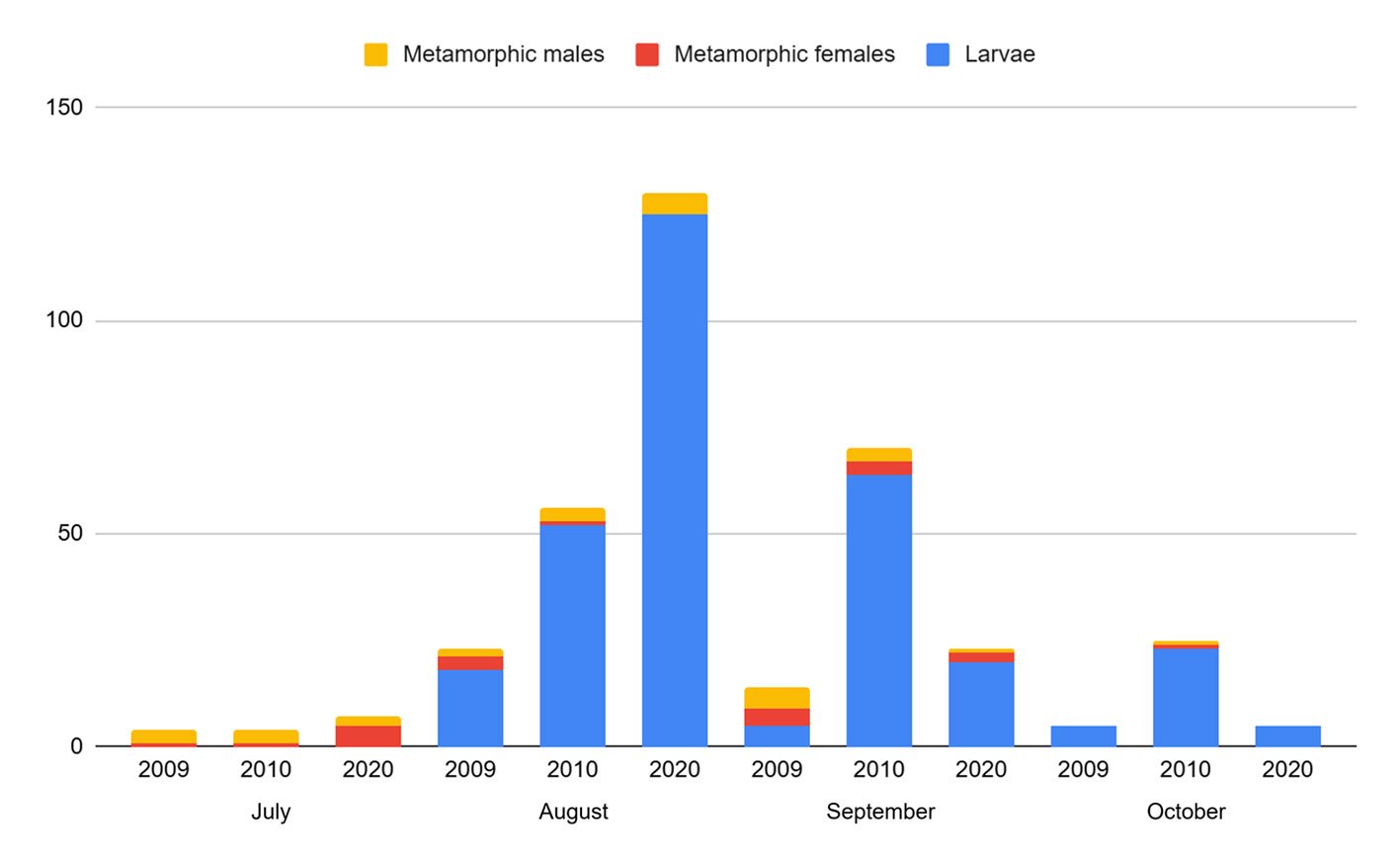
Table 2
Morphometric data (average, minimum, and maximum) of individuals analyzed histologically to determine sexual maturity. SVL = Snout-vent length, TL = total length (mm), and weight (g).
| Category | Metamorphic females | Metamorphic males | Larvae |
| Avg. SVL | 81.4 | 90.8 | 62.5 |
| Min. SVL | 60 | 60 | 50 |
| Max. SVL | 100 | 115 | 85 |
| Avg. TL | 156.1 | 167.9 | 114.6 |
| Min. TL | 130 | 110 | 85 |
| Max. TL | 180 | 220 | 155 |
| Avg. weight | 23.53 | 20.13 | 9.57 |
| Min. weight | 10 | 8 | 4 |
| Max. weight | 42 | 36 | 20 |
| Gonadal development (Yes/No) | Yes | Yes | No |
| Number of individuals | 14 | 24 | 14 |
Sexual maturity. Of the 52 dissected individuals, 24 were males, 14 females and 14 larvae. Males had an SVL ranging from 60 to 115 mm, females from 60 to 100 mm, and larvae from 50 to 85 mm (Table 2). According to the ANOVA, a significant association was found between size and the different age categories (p < 0.05). Through histological analysis, 38 individuals exhibited sexual development (Table 2). We determined that sexual maturity occurs at an SVL of 60 mm, as vitellogenic oocytes in females and mature sperm in males were observed at this size (Fig. 4).
Discussion
Our study on Ambystoma lermaense in Capilla Vieja provides critical insights into its population dynamics, sexual maturity, and conservation status. By situating these findings within a broader ecological and conservation context, we can deepen our understanding of the factors influencing the persistence of this species and its relatives. The gradual increase in population density from 0.021 individuals/m² in 2009 to 0.075 individuals/m² in 2020 is a positive indicator of stability. However, these densities remain substantially lower than those reported by Huacuz (2003) in the Reserva de la Biosfera Mariposa Monarca (2.3 individuals/m²). This stark contrast underscores the influence of habitat quality and protection on population viability. The Capilla Vieja site, despite being part of a protected natural area, is exposed to semi-intensive livestock activities and seasonal hydrological fluctuations, both of which could limit carrying capacity for A. lermaense.
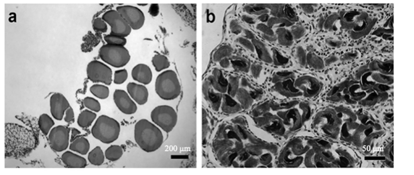
Examining densities and threats across 3 Ambystoma species provides valuable comparative insights: Ambystoma mexicanum, critically low densities in Xochimilco lake (0.001 individuals/m²) highlight severe impacts from urbanization and habitat degradation (Contreras et al., 2009). Ambystoma altamirani, densities ranging from 0.016 to 0.027 individuals/m² in trout-free streams in Estado de México suggest that invasive species exacerbate population declines (Lemos-Espinal et al., 1999). Ambystoma ordinarium, densities of 0.030-0.050 individuals/m² in Michoacán State highlight the challenges posed by deforestation and agricultural expansion (Aguilar-Miguel, 2005). These comparisons reinforce the role of protected areas in supporting higher population densities and the importance of mitigating threats in unprotected habitats.
The discovery that sexual maturity in A. lermaense occurs at a SVL of 60 mm aligns with findings for other facultatively paedomorphic Ambystoma species. Paedomorphosis, the retention of larval traits in adults, allows these salamanders to reproduce in aquatic habitats, potentially enhancing resilience in fragmented or fluctuating environments. However, the high proportion of juveniles (87%) in Capilla Vieja suggests a reliance on consistent recruitment, which could be disrupted by environmental changes.
The Capilla Vieja site is part of a connected watercourse system, but its fragmentation due to agricultural activities and seasonal stream drying limits habitat availability. Maintaining connectivity between breeding and non-breeding habitats is critical for sustaining gene flow and reducing local extinction risks. Lessons from the Reserva de la Biosfera Mariposa Monarca, where robust habitat connectivity supports high densities of this species, should guide management strategies for fragmented landscapes.
High-altitude amphibians like A. lermaense are particularly vulnerable to climate change. Rising temperatures and altered precipitation patterns could shrink suitable habitat ranges and exacerbate seasonal drying of streams. Proactive measures, such as restoring vegetation cover and monitoring hydrological changes, are necessary to mitigate these effects. While protected areas like the Reserva de la Biosfera Mariposa Monarca demonstrate the effectiveness of large-scale conservation, localized efforts are equally vital. Capilla Vieja’s inclusion in a protected area offers an opportunity to implement targeted interventions, such as: enhancing water quality through pollution control; reducing the impact of livestock on stream habitats; and introducing community-based conservation programs to engage local stakeholders.
The findings on A. lermaense reflect broader trends in amphibian conservation. Amphibians worldwide face similar threats of habitat degradation, invasive species, and climate change. This study contributes to the growing body of evidence that localized conservation actions, combined with broader protections, can stabilize and even enhance populations of threatened species. Future studies could explore: genetic diversity, assessing genetic variation in A. lermaense populations to evaluate the effects of fragmentation on genetic health. Behavioral ecology, investigating breeding behavior, dispersal patterns, and predator-prey dynamics to inform conservation strategies. Impact of invasive species, examining whether invasive species, such as trout, are encroaching on nearby A. lermaense habitats.
The relatively stable population density of Ambystoma lermaense in Capilla Vieja reflects its resilience but highlights the challenges posed by habitat degradation and fragmentation. Comparisons with other Ambystoma species and populations in protected areas underscore the importance of habitat quality and connectivity. To ensure the long-term survival of A. lermaense and its relatives, conservation efforts must integrate habitat restoration, community engagement, and climate adaptation strategies. As amphibians are critical indicators of ecosystem health, their protection benefits biodiversity and ecological integrity on a broader scale.
Acknowledgments
We gratefully acknowledge Conahcyt for the scholarship awarded to GL-B during his PhD studies in Biological Sciences at UNAM (2009–2011; registration number 161331). We also thank Gabriel Gutiérrez-Ospina for funding provided through GlaxoSmithKline, as well as the annual budget allocated to the Integrative Biology Laboratory by the Administrative Secretariat of the Institute of Biomedical Research, UNAM, which partially supported this project. Additional support was provided by DGAPA-UNAM (PAPIIT-UNAM, IN208024) and Secihti(CBF-2025-G-418) to GP-O. We are grateful to Fernando Arana Magallón, coordinator of the Biological and Aquaculture Research Center of Cuemanco (CIBAC-UAM-X), for his assistance with fieldwork, laboratory work, and specimen collection. We also thank Miguel Tapia-Rodríguez, head of the Microscopy Unit at IIB-UNAM, for his support in figure design. We acknowledge Semarnat for the permits granted for this study (Nos. SGPA/DGVS/00417/09, SGPA/DGVS/02729/10, and SGPA/DGVS/03197/20). Finally, we thank the two anonymous reviewers and the section editor for their valuable comments, which improved the manuscript.
References
Aguilar-Miguel, X. (2005). Ambystoma ordinarium. Algunas especies de anfibios y reptiles contenidos en el Proyecto de Norma Oficial Mexicana PROY-NOM-059-ECOL-2000. Facultad de Ciencias, Centro de Investigación en Recursos Bióticos, Universidad Autónoma del Estado de México.
Aguilar-Miguel, X., Legorreta-Balbuena, G., & Casas-Andreu, G. (2009). Reproducción ex situ en Ambystoma granulosum y Ambystoma lermaense (Amphibia: Ambystomatidae). Acta Zoológica Mexicana, 25, 443–454. https://doi.org/10.21829/azm.2009.253652
Blaustein, A. R., & Wake, D. B. (1990). Declining amphibian populations: a global phenomenon? Trends in Ecology & Evolution, 5, 203–204. https://doi.org/10.1016/0169-5347(90)90129-2
Semarnat (Secretaría de Medio Ambiente y Recursos Naturales). (2018). Acuerdo por el que se da a conocer el resumen del Programa de Manejo del Área Natural Protegida con la categoría de área de protección de recursos naturales cuencas de los ríos Valle de Bravo, Malacatepec, Tilostoc y Temascaltepec, Estado de México. Diario Oficial de la Federación. Normateca Ambiental. https://normatecambiental.org/2018/12/05/acuerdo-por-el-que-se-da-a-conocer-el-programa-de-manejo-del-area-natural-protegida-de-cuencas-de-los-rios-valle-de-bravo-malacatepec-tilostoc-y-temascaltepec-estado-de-mexico/
Contreras, V., Martínez-Meyer, E., Valiente, E., & Zambrano, L. (2009). Recent decline and potential distribution in the last known wild populations of the critically endangered Mexican Axolotl. Biological Conservation, 142, 2881–2885. https://doi.org/10.1016/j.biocon.2009.07.008
Dirzo, R., Ceballos, G., & Ehrlich, P. R. (2022). Circling the drain: the extinction crisis and the future of humanity. Philosophical Transactions of the Royal Society B, 377, 20210378. https://doi.org/10.1098/rstb.2021.0378
Egea-Serrano, A., Relyea, R. A., Tejedo, M., & Torralva, M. (2012). Understanding the impact of chemicals on amphibians: a meta-analytic review. Ecology and Evolution, 2, 1382–1397. https://doi.org/10.1002/ece3.249
Everson, K. M., Gray, L. N., Jones, A. G., Lawrence, N. M., Foley, M. E., Sovacool, K. L. et al. (2021). Geography is more important than life history in the recent diversification of the tiger salamander complex. Proceedings of the National Academy of Sciences, 118, e2014719118. https://doi.org/10.1073/pnas.2014719118
Grant, E. H. C., Miller, D. A. W., Schmidt, B. R., Adams, M. J., Amburgey, S. M., Chambert, T. et al. (2016). Quantitative evidence for the effects of multiple drivers on continental-scale amphibian declines. Scientific Reports, 6, 25625. https://doi.org/10.1038/srep25625
Green, D. M. (2003). The ecology of extinction: population fluctuation and decline in amphibians. Biological Conservation, 111, 331–343. https://doi.org/10.1016/S0006-3207(02)00302-6
Heyer, W. R., Donnelly, M. A., McDiarmid, R. W., Hayek, A. C., & Foster, M. S. (1994). Measuring and monitoring biological diversity: standard methods for amphibians. Washington D.C.: Smithsonian Institution Press.
Huacuz-Elías, D. C. (2003). Estado de conservación de Ambystoma lermaense Taylor, (1940) en el Santuario Sierra Chincua de la Reserva de la Biosfera “Mariposa Monarca”. Revista de la Facultad de Biología de la UMSNH, 5, 51–63.
IUCN SSC Amphibian Specialist Group. (2015). Ambystoma lermaense (errata version published in 2020). The IUCN Red List of Threatened Species 2015: e.T1093A176771946. https://dx.doi.org/10.2305/IUCN.UK.2015-4.RLTS.T1093A176771946.en
Jacinto-Maldonado, M., González-Salazar, C., Basanta, M. D., García-Peña, G. E., Saucedo, B., Lesbarrères, D. et al. (2023). Water pollution increases the risk of chytridiomycosis in Mexican amphibians. EcoHealth, 20, 74–83. https://doi.org/10.1007/s10393-023-01631-0
Lemos-Espinal, J. A., Smith, G. R., Ballinger, R. E., & Ramírez-Bautista, A. (1999). Status of protected endemic salamanders (Ambystoma: Ambystomatidae: Caudata) in the transvolcanic belt of Mexico. British Herpetological Society Bulletin, 68, 1–4.
Lips, K. R., Reaser., J. K., & Young, B. (1999). Monitoreo de anfibios en América Latina: manual de protocolos. Herpetological Circular No. 30. https://amphibiaweb.org/resources/Anfibios.pdf
Mitchell, M. A. (2009). Anesthetic considerations for amphibians. Journal of Exotic Pet Medicine, 18, 40–49. https://doi.org/10.1053/j.jepm.2008.11.006
Pechmann, J. H., Scott, D. E., Semlitsch, R. D., Caldwell, J. P., Vitt, L. J., & Gibbons, J. W. (1991). Declining amphibian populations: the problem of separating human impacts from natural fluctuations. Science, 253, 892–895. https://doi.org/10.1126/science.253.5022.892
Pounds, J. (2001). Climate and amphibian declines. Nature, 410, 639–640. https://doi.org/10.1038/35070683
Reilly, S. M., & Brandon, R. A. (1994). Partial paedomorphosis in the Mexican stream ambystomatids and the taxonomic status of the genus Rhyacosiredon Dunn. Copeia, 1994, 656–662. https://doi.org/10.2307/1447181
Rentería, G., Cota, R. G., & Ortega, E. (2005). Descripción del medio natural de la cuenca del Valle de Bravo, Estado de México. Jiutepec, Morelos: Instituto Mexicano de Tecnología del Agua.
Robles-Mendoza, C., García-Basilio, C., Cram-Heydrich, S., Hernández-Quiroz, M., & Vanegas-Pérez, C. (2009). Organophosphorus pesticides effect on early stages of the axolotl Ambystoma mexicanum (Amphibia: Caudata). Chemosphere, 74, 703–710. https://doi.org/10.1016/j.chemosphere.2008.09.087
Rubio-Limonta, M., & Silveira-Coffigny, R. (2009). Bienestar de los animales acuáticos, con fines de control sanitario. REDVET. Revista Electrónica de Veterinaria, 10. https://www.redalyc.org/pdf/636/63617143009.pdf
Stuart, S. N., Chanson, J. S., Cox, N. A., Young, B. E., Rodrigues, A. S., Fischman, D. L. et al. (2004). Status and trends of amphibian declines and extinctions worldwide. Science, 306, 1783–1786. https://doi.org/10.1126/science.1103538
Taylor, E. H. (1940). A new Rhyacosiredon (Caudata) from western México. Herpetologica, 1, 171–176.
Williams, L. R., Crosswhite, D. L., & William, M. G. (2002). Short-term effect of riparian disturbance on Desmog-
nathus brimleyorum (Plethodontidae) at natural spring in Oklahoma, U.S.A. The Southwestern Naturalist, 47,
611–613. https://doi.org/10.2307/3672667

A contribution to the diversity and distribution of the genus Scleroderma (Boletales: Sclerodermataceae) in Mexico
Contribución a la diversidad y distribución del género Scleroderma (Boletales: Sclerodermataceae) en México
Erika Cecilia Pérez-Ovando a, Bernardo Águila b, Wilfredo A. Matamoros a, Olivia Ayala-Vásquez c, d, Roberto Garibay-Orijel b, *
a Universidad Autónoma de Ciencias y Artes de Chiapas, Instituto de Ciencias Biológicas, Programa de Doctorado en Ciencias en Biodiversidad y Conservación de Ecosistemas Tropicales, Libramiento Norte Poniente, Col. Lajas Maciel, 29039 Tuxtla Gutiérrez, Chiapas, Mexico
b Universidad Nacional Autónoma de México, Instituto de Biología, Departamento de Botánica, Tercer Circuito s/n, Ciudad Universitaria, Coyoacán, 04510 Ciudad de México, Mexico
c Secretaría de Ciencia, Humanidades, Tecnología e Innovación, Av. Insurgentes Sur 1582, Col. Crédito Constructor, Benito Juárez, 03940 Ciudad de México, Mexico
d Colegio de Postgraduados, Campus Montecillo, Departamento de Edafología, Laboratorio de Micorrizas, 56230 Montecillo, Estado de México, Mexico
* Corresponding author: rgaribay@ib.unam.mx (R. Garibay-Orijel)
Received: 14 March 2025; accepted: 04 November 2025
Abstract
The order Boletales is one of the most diverse and widespread groups of macromycetes globally, with the genus Scleroderma being a significant representative. Despite the ecological, medical, and biocultural importance of this genus, studies on its systematics and genetic diversity in Mexico are scarce. Here, we studied the diversity and distribution of Scleroderma in Mexico using all available information (voucher registers, voucher DNA, and environmental DNA). A total of 120 nrITS DNA sequences from different species were analyzed, including 27 from environmental samples, while the remaining sequences were obtained from public databases. In Mexico, 15 Scleroderma species have been cited by morphological taxonomy, while molecular evidence suggest around 24 taxa. Phylogenetic analyses divided the genus into 4 main clades. Clade A corresponds to section Scleroderma and includes S. albidum s.l., S. areolatum, and S. cepa/laeve; clade B includes species of section Sclerangium and S. anomalosporum; clade C includes only S. dictyosporum; and clade D corresponds to section Reticulatae and includes S. bovista, S. citrinum s.l., and S. meridionale. The presence of S. capeverdeanum s.l. and S. venenatum is reported for the first time in Mexico.
Keywords: Environmental DNA; Soil; Macromycetes; Biogeography
Resumen
El orden Boletales constituye uno de los grupos de macromicetos más diversos y ampliamente distribuidos, con el género Scleroderma como un representante significativo. A pesar de su relevancia, los estudios sobre su sistemática y diversidad en México son escasos. En este trabajo analizamos la diversidad y distribución de Scleroderma en México a partir de toda la información disponible (registros de especímenes, DNA de esporomas y DNA ambiental). Se evaluaron 120 secuencias de DNA nrITS, de las cuales 27 corresponden a muestras ambientales; las restantes se obtuvieron de bases de datos públicas. Mientras que por taxonomía morfológica se han citado 15 especies de Scleroderma en el país, nuestros resultados sugieren aproximadamente 24 especies. Los análisis filogenéticos revelaron 4 clados principales: el clado A corresponde a la sección Scleroderma e incluye a S. albidum s.l., S. areolatum y S. cepa/laeve; el clado B incluye las especies de la sección Sclerangium y a S. anomalosporum; el clado C integra únicamente a S. dictyosporum; y el D corresponde a la sección Reticulatae, e incluye a S. bovista, S. citrinum s.l. y S. meridionale. Asimismo, se reporta por primera vez en México la presencia de S. capeverdeanum y S. venenatum.
Palabras clave: DNA ambiental; Suelo; Macromicetos; Biogeografía
Introduction
The estimation of the global diversity of fungi is still under debate, conservative authors propose a range between 1.5 and 3.8 million species (Hawksworth, 1991; Hawksworth & Lücking, 2017). However, current knowledge about fungal diversity is still insufficient, as many of the species have not been described or detected through their sporomes (Tedersoo et al., 2014). Furthermore, in Mexico the complex topography, strong habitat variability, and convergence of Nearctic and Neotropical biota contribute to a high fungal diversity characterized by many cryptic lineages (Cifuentes-Blanco et al., 1997; Sánchez-Ramírez, 2015). Consequently, morphological traits of fungi are insufficient in many taxa to detect hidden diversity.
In recent decades, tools such as metabarcoding have been used to improve species detection, particularly from environmental samples such as air, water, and soil (Heeger et al., 2018; Korpelainen et al., 2017; Tedersoo et al., 2014, 2022). Regarding macromycetes, these techniques have enhanced our understanding of the diversity of genera with medical, edible, economic, or cultural importance, such as Suillus and Tuber (Bonito et al., 2010; Tao et al., 2024) and have clarified ecological relationships between Boletus and the soil microbiota (Santolamazza-Carbone et al., 2023). However, the diversity of other groups such as Scleroderma remains underestimated.
The genus Scleroderma described by Persoon (1801) belongs to the family Sclerodermataceae within the Boletales (Binder & Bresinsky, 2002; Kirk et al., 2008). Species in this genus develop ectomycorrhizal associations with temperate and tropical plants such as Coccoloba, Eucalyptus, Fagus, Pinus, and Quercus, among others (Guzmán et al., 2013; Lu et al., 1998; Rincón et al., 2001; Sims et al., 1995). It has been estimated that the Sclerodermatineae originated 66 million years ago, at the end of the Cretaceous, while its main genera diversified around the middle Cenozoic. Consequently, Scleroderma is presumed to have originated approximately 38.37 million years ago, at the end of the Eocene (Wilson et al., 2012).
Several species of Scleroderma are considered edible, toxic, or medicinal. For instance, S. citrinum, S. flavidum,and S. yunnanense stand out as edible mushrooms in China (Wang et al., 2004; Zhang et al., 2013), while S. citrinum, S. dictyosporum,and S. polyrhizum are consumed in India (Karun et al., 2022). The edibility of S. laeve and S. texense has been documented for Mexico (Cortés-Pérez et al., 2021; De Ávila et al., 1980). Moreover, toxicity assays using Artemia franciscana larvae confirmed that Mexican specimens of S. texense do not exhibit toxic effects, supporting their local use as edible fungi (Ruiz-González et al., 2017). On the other hand, S. areolatum, S. bovista, S. cepa, S. citrinum, S. flavidum, S. polyrhizum,and S. verrucosum are considered medicinal in China (Dai & Yang, 2008). In Mexico, S. areolatum, S. nitidum, and S. verrucosum are used to stop bleeding from wounds (Guzmán et al., 2013). Conversely, some authors have classified species like S. albidum, S. areolatum, S. cepa, and S. venenatum as toxic (Guzmán, 1970; Sato et al., 2020; Yao et al., 2023; Zhang et al., 2020; Zhong et al., 2021).
In soil restoration projects, Scleroderma plays a significant role in maintaining and establishing ectomycorrhizal hosts. Its species improve the establishment, growth, and functional traits of their hosts (Bullaín-Galardis et al., 2024). For this reason, species such as S. citrinum, S. polyrhizum, S. texense, and S. verrucosum have been used to inoculate native trees during revegetation efforts in abandoned agricultural lands or arid soils (Pera & Parladé, 2005; Valdés-Ramírez et al., 2010). Even tropical species such as S. bermudense has been inoculated in Coccoloba uvifera to alleviate salinity stress and restore coastal dunes (Bandou et al., 2006; Bullaín-Galardis et al., 2024).
From a morphological perspective, Scleroderma was divided into 3 sections by Guzmán (1967, 1970) based on microscopic diagnostic characters such as basidiospore ornamentation and the structure of generative hyphae: section Aculeatispora characterized by the presence of echinulate basidiospores and the absence of clamp connections; section Sclerangium with subreticulate, subechinulate or echinulate basidiospores and abundant clamp connections; finally, section Scleroderma with reticulate basidiospores and few clamp connections. However, a change in the name of the sections Aculeatispora and Scleroderma to sections Scleroderma and Reticulatae, respectively, was later proposed (Guzmán et al., 2013). Some molecular studies partially agreed with this classification and reported new species based on some DNA regions such as nrITS (Nouhra et al., 2012; Phosri et al., 2009; Rusevska et al., 2014; Wu et al., 2023).
Scleroderma has around 100 species names registered in Index Fungorum (https://www.indexfungorum.org) and MycoBank (https://www.mycobank.org/). In Scleroderma, species complexes are not exclusively composed of cryptic taxa, while some species are morphologically indistinguishable and can only be separated using molecular data, many others can be reliably distinguished based on macroscopic and microscopic characters. However, some species such as S. meridionale, S. polyrhizum, and S. septentrionale represent species complexes that are being delimited through phylogenetic studies (Ortíz-Rivero et al., 2021). This highlights the importance of integrating morphological and molecular evidence to achieve accurate species delimitation within the genus.
Although phylogenetic and molecular studies for the genus exist worldwide (Nouhra et al., 2012; Phosri et al., 2009; Rusevska et al., 2014; Yang et al., 2025), only morphological studies have been carried out in Mexico, where 15 morphospecies have been reported: S. albidum, S. areolatum, S. bermudense, S. bovista, S. cepa, S. citrinum, S. hypogaeum, S. mexicana, S. michiganense, S. nitidum, S. polyrhizum, S. pseudostipitatum, S. texense, and S. verrucosum (Guzmán, 1970; Guzmán et al., 2013; Guzmán-Dávalos & Guzmán, 1985). Additionally, S. guzmanii was described by Ortíz-Rivero et al. (2021), and S. cepa s.l. was recently reported through phylogenetic analysis associated with Carya illinoinensis (Sánchez-Ledesma et al., 2023).
Due to the uncertainty regarding the diversity of Scleroderma species in Mexico, we conducted a comprehensive study integrating all genetic and geographic information available for the genus in the country. This approach is key to obtaining a more complete view of Scleroderma diversity in Mexico.
Materials and methods
Soil environmental DNA (eDNA) sampling was carried out in the northeast, center, south, and southeast of Mexico (Fig. 1C) from 2019 to 2021, as part of the Global Soil Mycobiome Consortium Project (Tedersoo et al., 2021). A total of 73 locations in the states of Aguascalientes, Campeche, Chiapas, Coahuila, Hidalgo, Jalisco, Mexico City, Michoacán, Morelos, Nuevo León, Oaxaca, Puebla, Quintana Roo, Estado de Mexico, Tabasco, Tlaxcala, Veracruz, and Yucatán, were sampled. In each locality, we collected 40 soil cores around an area of 2,500 m2. Each soil core was retrieved with a polyvinyl tube (5 cm diameter and 10 cm depth) to take the organic horizon and the first part of the mineral horizon, avoiding litter. Afterwards, these were combined and homogenized to form a composite sample (~ 1 kg). Composite samples were placed in Ziploc bags (~ 250 g), dried and stored at 5 °C.
DNA extraction was performed as described in Tedersoo et al. (2021). Polymerase chain reactions (PCR) were performed to amplify the internal transcribed spacer region of the nuclear ribosomal DNA (nrITS) with the universal eukaryotic primers ITS9mun and ITS4ngsUni, according to the methods and conditions in Tedersoo and Anslan (2019). PCR libraries were constructed and sequenced in the PacBio Sequel II platform at the University of Oslo. The resulting sequences were demultiplexed, quality filtered chimeric sequences were removed, OTUs clustered at 98% similarity, and taxonomically annotated as described in Tedersoo et al. (2021). The most abundant sequence of each OTU was selected as its representative sequence and used for further analysis.
The resulting Scleroderma DNA sequences from soil were complemented with sequences retrieved from GenBank (Sayers et al., 2024) derived from voucher specimens and ectomycorrhizae. Our final dataset contained 120 nrITS sequences of which 27 correspond to eDNA and voucher specimens and 93 were retrieved from GenBank (Table 1). We used 2 sequences of Tremellogaster surinamensis (Wilson et al., 2011) as an outgroup to root the Scleroderma phylogeny. We aligned the DNA sequences with MAFFT with the FFT-NS-i algorithm with 1,000 repetitions implemented in Geneious Prime. The resulting alignment was manually edited and trimmed. The final alignment had 768 sites, including gaps.
The best nucleotide substitution model for our alignment (HKY + I + Gama) was selected based on the corrected Akaike information criterion (AICc; Burnham & Anderson, 2002) inferred in jModelTest (Darriba et al., 2012). We inferred phylogenetic relationships based on Bayesian and Maximum likelihood approaches. Both analyses were performed in MrBayes 6.1 and PHYML implemented in Geneious Prime. Maximum likelihood support was estimated with 1,000 bootstrap pseudo-replicates (MLB) (Felsenstein, 1985), leaving the rest of parameters as default. For the Bayesian inference, we ran 4 simultaneous Monte Carlo Markov Chains (MCMC) for 10 M generations, sampling every 1,000 trees.
Table 1
nrITS DNA sequences obtained from environmental soil samples and GenBank used for phylogenetic analysis.
| Species | GenBank access code | Country | Reference |
| Scleroderma albidum | PP582969 | India | Unpublished** |
| Scleroderma albidum | OR656734 | Spain | Unpublished** |
| Scleroderma albidum | KJ676532 | Brazil | Montagner et al., 2015 |
| Scleroderma albidum s.l.* | PV232154 | Mexico | This study |
| Scleroderma albidum s.l.* | PV232155 | Mexico | This study |
| Scleroderma albidum s.l.* | PV232156 | Mexico | This study |
| Scleroderma anomalosporum Type | NR147662 | Brazil | Baseia et al., 2016 |
| Scleroderma areolatum | FM213352 | USA | Phosri et al., 2009 |
| Scleroderma areolatum | EU784407 | Brock et al., 2009 | |
| Scleroderma areolatum | HF933231 | Macedonia | Rusevska et al., 2014 |
| Scleroderma areolatum | KC152224 | Mexico | Unpublished** |
| Scleroderma areolatum | KY574379 | Mexico | Unpublished** |
| Scleroderma areolatum | PV211138 | Mexico | Unpublished** |
| Scleroderma areolatum* | PV232141 | Mexico | This study |
| Scleroderma bermudense* | PV232132 | Mexico | This study |
| Scleroderma bermudense* | PV232133 | Mexico | This study |
| Scleroderma bermudense* | PV232142 | Mexico | This study |
| Scleroderma bermudense* | PV232143 | Mexico | This study |
| Scleroderma bermudense* | PV232144 | Mexico | This study |
| Scleroderma bermudense | OQ351731 | Cuba | Unpublished** |
| Scleroderma bermudense | OQ351725 | Cuba | Unpublished** |
| Scleroderma bermudense | OQ351721 | Cuba | Unpublished** |
| Scleroderma bermudense | KJ209672 | Senegal | Unpublished** |
| Scleroderma bermudense | KJ209674 | France | Unpublished** |
| Scleroderma aff. bermudense sp. 8* | PV232136 | Mexico | This study |
| Scleroderma aff. bermudense sp. 8* | PV232137 | Mexico | This study |
| Scleroderma aff. bermudense sp. 8* | PV232138 | Mexico | This study |
| Scleroderma aff. bermudense sp. 9* | PV232134 | Mexico | This study |
| Scleroderma aff. bermudense sp. 10* | PV232135 | Mexico | This study |
| Table 1. Continued | |||
| Species | GenBank access code | Country | Reference |
| Scleroderma bovista | KU739419 | Spain | Fernández-Miranda, 2014 |
| Scleroderma bovista | FM213340 | Spain | Phosri et al., 2009 |
| Scleroderma bovista | HF933235 | Macedonia | Rusevska et al., 2014 |
| Scleroderma bovista | HF933242 | Serbia | Rusevska et al., 2014 |
| Scleroderma cf. bovista | FM213339 | USA | Phosri et al., 2009 |
| Scleroderma camassuense Type | NR147663 | Brazil | Baseia et al., 2016 |
| Scleroderma capeverdeanum Type | NR164545 | Cape verde | Crous et al., 2016 |
| Scleroderma capeverdeanum | KU747111 | Cape verde | Crous et al., 2016 |
| Scleroderma capeverdeanum s.l.* | PV232145 | Mexico | This study |
| Scleroderma capeverdeanum s.l.* | PV232157 | Mexico | This study |
| Scleroderma cepa | OR882638 | USA | Unpublished** |
| Scleroderma cepa | EU784411 | Brock et al., 2009 | |
| Scleroderma cepa | OP743680 | USA | Unpublished** |
| Scleroderma cepa s.l. | MZ092921 | Mexico | Sánchez-Ledesma et al., 2023 |
| Scleroderma citrinum | FM213344 | USA | Phosri et al., 2009 |
| Scleroderma citrinum | KJ679575 | Brazil | Montagner et al., 2015 |
| Scleroderma citrinum | KJ679576 | Brazil | Montagner et al., 2015 |
| Scleroderma aff. citrinum* | PV232139 | Mexico | This study |
| Scleroderma columnare | AB459519 | Thailand | Ruankaew-Disyatat et al., 2016 |
| Scleroderma columnare | AB459512 | Thailand | Ruankaew-Disyatat et al., 2016 |
| Scleroderma dictyosporum | FJ840444 | Burkina Faso | Sanon et al., 2009 |
| Scleroderma dictyosporum | FJ840442 | Burkina Faso | Sanon et al., 2009 |
| Scleroderma dictyosporum | FJ840443 | Burkina Faso | Sanon et al., 2009 |
| Scleroderma dictyosporum | FJ840449 | Burkina Faso | Sanon et al., 2009 |
| Scleroderma duckei | KX792086 | Brazil | Baseia et al., 2016 |
| Scleroderma duckei Type | NR147664 | Brazil | Baseia et al., 2016 |
| Scleroderma dunensis Type | NR147646 | Brazil | Crous et al., 2016 |
| Scleroderma dunensis | KU747112 | Brazil | Crous et al., 2016 |
| Scleroderma dunensis | KU747114 | Brazil | Crous et al., 2016 |
| Scleroderma erubescens Type | OQ554978 | China | Wu et al., 2023 |
| Scleroderma erubescens | OQ554976 | China | Wu et al., 2023 |
| Scleroderma geaster | MT270642 | Spain | Ortiz-Rivero et al., 2021 |
| Scleroderma geaster | MT270640 | Portugal | Ortiz-Rivero et al., 2021 |
| Scleroderma guzmanii | MT270647 | Mexico | Ortiz-Rivero et al., 2021 |
| Scleroderma guzmanii Type | NR176725 | USA | Ortiz-Rivero et al., 2021 |
| Scleroderma furfuraceum Type | NR186993 | Russia | Rebriev & Zvyagina, 2022 |
| Scleroderma laeve | EU718117 | Wilson et al., 2011 | |
| Scleroderma laeve | ON212388 | South Korea | Cho et al., 2022 |
| Scleroderma meridionale | HF933238 | Macedonia | Rusevska et al., 2014 |
| Table 1. Continued | |||
| Species | GenBank access code | Country | Reference |
| Scleroderma meridionale | MG367369 | Italy | Leonardi et al., 2018 |
| Scleroderma meridionale | MG264160 | Italy | Leonardi et al., 2018 |
| Scleroderma meridionale | EU718121 | USA | Unpublished** |
| Scleroderma michiganense | FM213348 | USA | Phosri et al., 2009 |
| Scleroderma michiganense | FM213347 | USA | Phosri et al., 2009 |
| Scleroderma michiganense | FM213346 | USA | Phosri et al., 2009 |
| Scleroderma nastii | ON212391 | South Korea | Cho et al., 2022 |
| Scleroderma nitidum | KU759906 | Brazil | Baseia et al., 2016 |
| Scleroderma nitidum | KU759908 | Brazil | Baseia et al., 2016 |
| Scleroderma patagonicum | KY462453 | Argentina | Truong et al., 2017 |
| Scleroderma patagonicum | HQ688789 | Argentina | Noura et al., 2012 |
| Scleroderma polyrhizum | MT270661 | USA | Ortiz-Rivero et al., 2021 |
| Scleroderma polyrhizum | MT270662 | Spain | Ortiz-Rivero et al., 2021 |
| Scleroderma separatum | OQ554975 | China | Wu et al., 2023 |
| Scleroderma separatum | OQ554973 | China | Wu et al., 2023 |
| Scleroderma septentrionale | FM213338 | USA | Phosri et al., 2009 |
| Scleroderma septentrionale | FM213336 | Sweden | Phosri et al., 2009 |
| Scleroderma cf. septentrionale | FM213337 | USA | Phosri et al., 2009 |
| Scleroderma sinnamariense | FM213358 | Thailand | Phosri et al., 2009 |
| Scleroderma sinnamariense | AB908177 | India | Unpublished** |
| Scleroderma sinnamariense | HQ687222 | Thailand | Unpublished** |
| Scleroderma squamulosum | OQ554980 | China | Wu et al., 2023 |
| Scleroderma squamulosum Type | OQ554979 | China | Wu et al., 2023 |
| Scleroderma suthepense Type | NR132871 | Thailand | Kumla et al., 2013 |
| Scleroderma texense | MT270650 | USA | Ortiz-Rivero et al., 2021 |
| Scleroderma texense | MT270649 | USA | Ortiz-Rivero et al., 2021 |
| Scleroderma texense* | PV232140 | Mexico | This study |
| Scleroderma venenatum | OQ750238 | China | Unpublished** |
| Scleroderma venenatum | JF273540 | China | Zhang et al., 2020 |
| Scleroderma venenatum | KC52225 | Mexico | Unpublished** |
| Scleroderma venenatum | MH513631 | China | Zhang et al., 2020 |
| Scleroderma venenatum | OM874611 | Russia | Rebriev & Zvyagina, 2022 |
| Scleroderma venenatum | OM874613 | Russia | Rebriev & Zvyagina, 2022 |
| Scleroderma venenatum | MH513632 | China | Zhang et al., 2020 |
| Scleroderma verrucosum | EU784415 | England | Brock et al., 2009 |
| Scleroderma verrucosum | HF933241 | Macedonia | Rusevska et al., 2014 |
| Scleroderma vinaceum | OQ554986 | China | Wu et al., 2023 |
| Scleroderma vinaceum Type | OQ554987 | China | Wu et al., 2023 |
| Scleroderma yunnanense | JQ639046 | China | Wu et al., 2023 |
| Table 1. Continued | |||
| Species | GenBank access code | Country | Reference |
| Scleroderma yunnanense | JQ639045 | China | Wu et al., 2023 |
| Scleroderma yunnanense | JQ639041 | China | Wu et al., 2023 |
| Scleroderma sp. 1* | PV232153 | Mexico | This study |
| Scleroderma sp. 2 | PV211140 | Mexico | Unpublished ** |
| Scleroderma sp. 3* | PV232158 | Mexico | This study |
| Scleroderma sp. 4* | PV232149 | Mexico | This study |
| Scleroderma sp. 4* | PV232150 | Mexico | This study |
| Scleroderma sp. 4* | PV232151 | Mexico | This study |
| Scleroderma sp. 4* | PV232152 | Mexico | This study |
| Scleroderma sp. 5* | PV232146 | Mexico | This study |
| Scleroderma sp. 6* | PV232147 | Mexico | This study |
| Scleroderma sp. 7* | PV232148 | Mexico | This study |
| Tremellogaster surinamensis | KT724170 | Colombia | Unpublished ** |
| Tremellogaster surinamensis | EU718127 | Wilson et al., 2011 |
* Sequences obtained from environmental soil samples. ** Unpublished GenBank sequences.
We visually assessed sampling stationarity in Tracer ver. 1.7 (Rambaut et al., 2018) and by the observed average standard deviation of split frequencies (< 0.01). Finally, we discarded 20% of the sampled trees as burn-in, resulting in a collection of 7,510 trees. A majority rule consensus tree and Bayesian posterior probabilities (BPP) were calculated with the post-burn-in trees. We visually compared topological congruence between replicates and inference methods and edited the final tree in FigTree ver 1.4.4 (Rambaut, 2018).
To determine the distribution and species richness of Scleroderma in Mexico, we used the occurrence of the clades in the 73 sampling sites (Fig. 1C). This information was complemented with the 2,349 records of Scleroderma for Mexico in the GBIF public database (GBIF.org, August 27, 2024) (Fig. 1B). Records at the genus level were excluded. Since the political division of the country is not suitable for understanding patterns and processes of biodiversity, a distribution map of the genus was created using the level IV ecoregions of Mexico (Conabio, 2008).
Results
The consensus tree shows that Scleroderma is divided into 4 main clades (A, B, C, and D) with medium to high MLB and BPP support values. The topology of the inferred phylogenetic trees was similar in both analyses. The Mexican species were distributed in clades A, B, and D (Fig. 2). Morphologically, 15 species reported in the literature are recognized for Mexico, 9 from GBIF records only. Scleroderma capeverdeanum s.l.and S. venenatum complex are recorded for the first time along with several unnamed clades from soil samples. Of the total number of species, the clades corresponding to S. areolatum, the S. bermudense complex and the S. capeverdeanum s.l. are recognized from specimen vouchers and eDNA sampling, which leads us to consider that the number of species for Mexico is around 24.
Clade A (MLB: 92% and BPP: 1) contains species such as S. areolatum, S. cepa/laeve, and S. verrucosum. Several species from soil samples are also grouped together. Among the species sequenced from specimen vouchers, mycorrhizae, and eDNA from Mexico is S. areolatum. The grouping of Mexican sequences within the S. capeverdeanum s.l. clade (MLB: 75% and BPP:0.70) stands out, as well as sequences within S. venenatum (MLB: 100% and BPP: 1). Clade B (MLB: 62%, BPP: 0.99) includes species such as S. guzmanii and S. polyrhizum. Its most diverse subclade comprises the S. bermudense complex (MLB: 56%, BPP: 0.8), which is sister to S. aff. bermudense (MLB: 80%, BPP: 0.99), along with numerous soil DNA sequences associated with these 2 taxa. Clade C (MLB: 100% and BPP: 1) only contains S. dictyosporum, a species distributed in Africa and Southeast Asia. Clade D (MLB: 81%, BPP: 1) includes the Mexican taxon S. aff. citrinum from soil DNA, which is sister to S. citrinum s.l.
Species of Scleroderma occur throughout Mexico (Fig. 1A, Table 2); however, there are no records for the states of Baja California Sur and Zacatecas (Fig. 1B). The records obtained from soil eDNA are mainly concentrated in the central states of the country such as Estado de México, Hidalgo, and Michoacán; as well as the Yucatán Peninsula (Fig. 1C).
Regarding the clades obtained by eDNA, we found that they are distributed in 3 main vegetation types that correspond to tropical broadleaf forest, subtropical broadleaf forest, and tropical coniferous forest (Table 3). The clades of S. aff. bermudense and S. bermudense complex are mainly distributed in tropical broadleaf forest and subtropical broadleaf forest, while S. capeverdeanum distributes in tropical coniferous forest and subtropical coniferous forest. In the case of S. areolatum, it was only sequenced tropical broadleaf forests soil. The Transmexican Volcanic Belt is the physiographic province with the highest diversity of Scleroderma, being S. areolatum, S. cepa, and S. citrinum the most common species (Fig. 1D, E, F). Meanwhile, the largest number of records corresponds to S. bermudense complex from the Yucatán Peninsula.
There are clades of Neotropical distribution that include basidiomes and eDNA sequences such as those found within the S. bermudense complex; both, its basidiomes and soil DNA come mainly from the Yucatán Peninsula. Some OTUs of S. bermudense complex were found abundantly in the soil, such as S. aff. bermudense sp. 8 with 3,877 sequences. However, S. aff. bermudense sp. 9 and S. aff. bermudense sp. 10, have small distribution areas, apparently restricted to Mexico (Table 2).
Regarding the distribution of Scleroderma in Mexican ecoregions, there are more reports in the temperate sierras and less in the warm-dry forests. The ecoregions corresponding to the great deserts of Mexico remain among the least explored (Fig. 1G). In the southeast there are more records of S. bermudense found in the warm-humid forests of the Yucatán Peninsula, and in smaller numbers in warm-humid forests of Chiapas, Tabasco, and Veracruz.
Discussion
Our phylogenetic analysis matches partially with the results obtained in former molecular studies reporting that Scleroderma is divided into 2 main clades (Phosri et al., 2009; Rusevska et al., 2014). However, it is more consistent with current phylogenies including a larger number of species such as those of Wu et al. (2023) and Yang et al. (2025), who also found 4 main clades. It also does not fully correspond with the sections proposed by Guzmán (1967, 1970).
Our phylogeny and that of Yang et al. (2025) are similar across all major clades; even while our study includes only ITS sequences. Clade A corresponds to section Scleroderma and includes S. albidum s.l., S. areolatum, and S. cepa/laeve. Guzmán (2013) proposed S. laeve as a synonym of S. albidum; however, our results suggest that, instead, it may be a synonym of S. cepa. This section also comprises S. erubescens, S. separatum, S. squamulosum, and S. vinaceum, which cluster with species assigned to section Scleroderma, traditionally characterized by echinulate basidiospores and the absence of clamp connections. Nevertheless, Wu et al. (2023) reported that both S. erubescens and S. separatum possess clamp connections. This suggests that section Scleroderma may not be exclusively composed of species without clamp connections.
Clade B includes species in Section Sclerangium and S. anomalosporum, a species with smooth basidiospores (Baseia et al., 2016). Clade C remains the same, including only S. dictyosporum. This species was formerly placed in section Scleroderma, now recognized as section Reticulatae; however, in our analysis it forms an independent clade. Clade D corresponds to section Reticulatae.
Similarly, Yang et al. (2025) concluded that basidiospore ornamentation is not a reliable character for distinguishing section Scleroderma from section Sclerangium. Many species in section Scleroderma may also produce subreticulate basidiospores (e.g., S. areolatum, S. cepa, and S. nastii), whereas several new species in section Sclerangium can produce echinulate basidiospores (e.g., S. navigatum, S. xanthochroum, and S. zengchengense). The authors further proposed that peridium thickness may serve as an additional distinguishing feature.
Our results suggest that the number of Scleroderma species in Mexico is greater than the 15 previously reported (Guzmán et al., 2013; Ortíz-Rivero et al., 2021; Sánchez-Ledesma et al., 2023). We reported for the first time S. capeverdeanum s.l.and S. venenatum, as well as 10 clades that do not match with species previously sequenced. Conservatively the diversity of Scleroderma for Mexico is around 24 taxa. The discrepancy between species richness in voucher specimens versus DNA sequences may be explained due to scarce formation of basidiomes or because most of the described species have not been sequenced (Tedersoo et al., 2014).
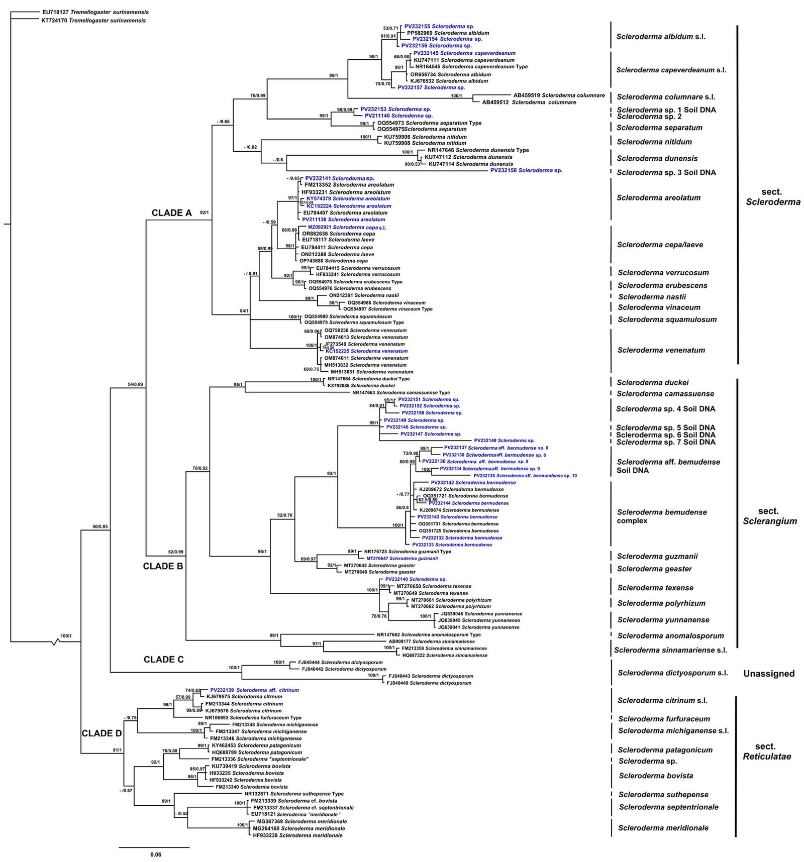
Table 2
Distribution and abundance of Scleroderma species obtained from soil samples.
| Species | Distribution | Abundance (Number of sequences) | Number of sites in Mexico |
| Scleroderma albidum s.l. | Estado de México | 5 | 1 |
| Scleroderma areolatum | Michoacán | 5 | 1 |
| Scleroderma bermudense | Quintana Roo and Yucatán | 164 | 2 |
| Scleroderma aff. bermudense sp. 8 | Morelos, Estado de México, Quintana Roo, and Yucatán | 3,877 | 5 |
| Scleroderma aff. bermudense sp. 9 | Yucatán | 1 | 1 |
| Scleroderma aff. bermudense sp. 10 | Yucatán | 10 | 1 |
| Scleroderma capeverdeanum s.l. | Hidalgo and Estado de México | 74 | 2 |
| Scleroderma aff. citrinum | Hidalgo | 1 | 1 |
| Scleroderma texense | Veracruz | 35 | 2 |
| Scleroderma sp. 1 | Veracruz | 3 | 1 |
| Scleroderma sp. 3 | Campeche and Quintana Roo | 3 | 2 |
| Scleroderma sp. 4 | Campeche, Michoacán and Yucatán | 33 | 8 |
| Scleroderma sp. 5 | Campeche and Yucatán | 33 | 5 |
| Scleroderma sp. 6 | Yucatán | 1 | 1 |
| Scleroderma sp. 7 | Campeche and Yucatán | 5 | 3 |
Table 3
Distribution of Scleroderma species in different types of vegetation.
| Species | Type of vegetation |
| Scleroderma albidum s.l. | Tropical coniferous forest |
| Scleroderma areolatum | Tropical broadleaf forest |
| Scleroderma bermudense | Subtropical broadleaf forest |
| Scleroderma aff. bermudense sp. 8 | Tropical broadleaf forest, subtropical broadleaf forest and tropical coniferous forest |
| Scleroderma aff. bermudense sp. 9 | Subtropical broadleaf forest |
| Scleroderma aff. bermudense sp. 10 | Subtropical broadleaf forest |
| Scleroderma capeverdeanum s.l. | Tropical coniferous forest and subtropical coniferous forest |
| Scleroderma aff. citrinum | Subtropical broadleaf forest |
| Scleroderma texense | Tropical coniferous forest |
| Scleroderma sp. 1 | Tropical coniferous forest |
| Scleroderma sp. 3 | Tropical broadleaf forest and subtropical broadleaf forest |
| Scleroderma sp. 4 | Tropical broadleaf forest, subtropical broadleaf forest, and tropical coniferous forest |
| Scleroderma sp. 5 | Tropical broadleaf forest and subtropical broadleaf forest |
| Scleroderma sp. 6 | Subtropical broadleaf forest |
| Scleroderma sp. 7 | Tropical broadleaf forest and subtropical broadleaf forest |
In the case of some OTUs of the S. bermudense complex, they could be considered endemic to Mexico, as they were only recorded at 1 sampling site. Other studies have reported that S. bermudense represents one of the most abundant endemic taxa in the Caribbean, mainly associated with Coccoloba uvifera (Bâ et al., 2024; Põlme et al., 2017). This association is mediated by the environmental stress of the coastal dunes where they develop, which causes a high specificity of the symbiosis (Bâ et al., 2024; Põlme et al., 2017). We found several clades of S. bermudense s.l.with high genetic differentiation not associated with Coccoloba species. Thus, there is a species complex associated with S. bermudense with an unsolved taxonomy and ecology in the Yucatán Peninsula.
Species such as S. areolatum and S. cepa have been recorded throughout the country through their basidiomes (Guzmán & Herrera, 1973; Guzmán et al., 2013). Scleroderma areolatum was reported from Durango, Guerrero, Hidalgo, Jalisco, México City, Michoacán, Nuevo León, Oaxaca, Puebla, and Veracruz (Guzmán & Herrera, 1973). Through ITS analysis it has been confirmed that S. cepa s.l. is an ectomycorrhizal symbiont of pecan trees in Chihuahua and Coahuila and that it is possibly a species complex (Sánchez-Ledesma et al., 2023). However, the type specimens of both species have not been sequenced, so it is important to carry out their type studies given the importance they can have in agroecosystems. In fact, species complexes indicating cryptic lineages in fungi are common (Sánchez-Ramírez, 2015) and may include taxa that can be morphologically distinguished, as well as cryptic species that are only discernible through molecular data, as this study found for the S. albidum, S. bermudense, and S. cepa complexes.
We recorded for the first time S. venenatum in Mexico, a species considered toxic in China (Zhang et al., 2020). The presence of this species in the country is particularly relevant given that some Scleroderma species are traditionally consumed in Mexico. For example, the consumption of S. laeve has been reported in Morelos and S. texense in Oaxaca (Cortés-Pérez et al., 2021; De Ávila et al., 1980). In contrast, S. venenatum was recorded in Querétaro and can be distinguished from edible species by its sessile, brown to grayish brown basidiomes and well-developed rhizomorphs (Zhang et al., 2020). Regarding the identity of the species that have been reported as edible in Mexico, their identification was only carried out with morphology and given their importance in cultural contexts, it would be advisable to obtain molecular data from the basidiomes to corroborate their identity.
A higher diversity of Scleroderma in the Transmexican Volcanic Belt shows that, while for other organisms the system represents a barrier or a filter, fungi use it as a corridor (Gómez-Reyes et al., 2018). In this region, the complex topography, habitat variability, and the convergence between Nearctic and Neotropical biota contribute to a higher diversity of fungal species in general (Cifuentes-Blanco et al., 1997) and in particular for Scleroderma.
Acknowledgements
The first author thanks the Secretaría de Ciencia, Humanidades, Tecnología e Innovación (Secihti) for the scholarship granted (CVU 415474) and the Instituto de Ciencias Biológicas, Universidad Autónoma de Ciencias y Artes de Chiapas (UNICACH) for all the facilities provided. This article contains part of the results of the PhD thesis project for the Doctorado en Ciencias en Biodiversidad y Conservación de Ecosistemas Tropicales (UNICACH). This research was funded by UNAM-PAPIIT IV200223 grant awarded to RGO.
References
Bâ, A. M., Séne, S., Manokari, M., Galardis, M. B., Sylla, S. N., Selosse, M. A. et al. (2024). Coccoloba uvifera L. associated with Scleroderma bermudense Coker: a pantropical ectomycorrhizal symbiosis used in restoring of degraded coastal sand dunes. Mycorrhiza, 34, 375–389. https://doi.org/10.1007/s00572-024-01170-8
Bandou, E., Lebailly, F., Muller, F., Dulormne, M., Toribio, A., Chabrol, J. et al. (2006). The ectomycorrhizal fungus Scleroderma bermudense alleviates salt stress in seagrape (Coccoloba uvifera L.) seedlings. Mycorrhiza, 16, 559–565. https://doi.org/10.1007/s00572-006-0073-6
Baseia, I. G., Silva, B. D. B., Ishikawa, N. K., Soares, J. V. C., Franca, I. F., Ushijima, S. et al. (2016). Discovery or extinction of new Scleroderma species in Amazonia? Plos One, 11, 1–19. https://doi:10.1371/journal.pone.0167879
Binder, M., & Bresinsky, A. (2002). Derivation of a polymorphic lineage of Gasteromycetes from boletoid ancestors. Mycologia, 94, 85–98. https://doi.org/10.1080/15572536.2003.11833251
Bonito, G. M., Gryganskyi, A. P., Trappe, J. M., & Vilgalys, R. (2010). A global meta-analysis of Tuber ITS rDNA sequences: species diversity, host associations and long-distance dispersal. Molecular Ecology, 19, 4994–5008. https://doi.org/10.1111/j.1365294X.2010.04855.x
Brock, P. M., Doring, H., & Bidartondo, M. I. (2009). How to know unknown fungi: the role of a herbarium. New Phytologist, 181, 719–724. https://doi.org/10.1111/j.1469-8137.2008.02703.x
Bullaín-Galardis, M. M., López-Sánchez, R. C., Pruneau, L., Eichler-Lobermann, B., Fall, F., & Bâ, A. M. (2024). Using the ectomycorrhizal symbiosis between Coccoloba uvifera L. and Scleroderma bermudense Coker to restore a degraded coastal sand dune in Cuba. Trees, 38, 127–138. https://doi.org/10.1007/s00468-023-02470-w
Burnham, K., & Anderson, D. (2002). Model selection and multimodel inference: a practical information-theoretic approach. New York: Springer.
Cho, S., Kwag, Y., Han, S., Lee, D., & Kim, C. (2022). Two new records of Scleroderma species (Sclerodermataceae, Boletales) in South Korea. The Korean Journal of Mycology, 50, 115–123. https://doi.org/10.4489/KJM.20220011
Cifuentes-Blanco, J., Villegas-Ríos, M., Villarreal-Ordaz, J. L., & Sierra Galván, S. (1997). Diversity of macromycetes in pine-oak forests in the Neovolcanic Axis, Mexico. In M. E. Palm, & I. H. Chapela (Eds.), Mycology in sustainable development: expanding concepts, vanishing borders (pp. 111–121). Boone, North Carolina: Parkway Publishers, Inc.
Conabio (Comisión Nacional para el Conocimiento y Uso de la Biodiversidad). (2008). Ecorregiones terrestres de México. Escala 1:1000000. México. Digital cartographic dataset. Mexico. https://www.conabio.gob.mx/informacion/gis/
Cortés-Pérez, A., Pérez-Pacheco, C. K., Yescas-Arreola, E., & Ramírez-Cruz, V. (2021). Primer registro de Scleroderma texense (Boletales, Sclerodermatinae) como una especie comestible en la Sierra Sur de Oaxaca, México. Scientia Fungorum, 52, 1–8. https://doi.org/10.33885/sf.2021.52.1386
Crous, P. W., Wingfield, M. J., Richardson, D. M., Le Roux, J. J., Strasberg, D., Edwards, J. et al. (2016). Fungal planet description sheets. Persoonia, 36, 316–458. https://doi:10.3767/003158516X692185.
Dai, Y. C., & Yang, Z. L. (2008). A revised checklist of medicinal fungi in China. Mycosystema, 27, 801–824.
Darriba, D., Taboada, G. L., Doallo, R., & Posada, D. (2012). jModelTest 2: more models, new heuristics and parallel computing. Nature Methods, 9, 772. http://doi:0.1038/nmeth.2109
De Ávila, A. B., Welden, A. L., & Guzmán, G. (1980). Notes on the ethnomycology of Hueyapan, Morelos, México. Journal of Ethnopharmacology, 2, 311–321. https://doi.org/10.1016/S0378-8741(80)81013-0
Felsenstein, J. (1985). Confidence limits on phylogenies: an approach using the bootstrap. Evolution, 39, 783–791. http//doi:10.1111/j.1558-5646.1985.tb00420.x
Fernández-Miranda, C. E. (2014). Hongos ectomicorrícicos de plantas leñosas en terrenos degradados de Asturias por actividad minera e industrial (Ph.D. Thesis). Universidad de Oviedo. Oviedo, España.
GBIF.org (2024). 27 August 2024 GBIF Occurrence Download https://doi.org/10.15468/dl.bbmwbt
Gómez-Reyes, V. M., Vázquez-Marrufo, G., Ortega-Gómez, A. M., & Guevara-Guerrero, G. (2018). Ascomicetos hipogeos de la región occidental del Sistema Volcánico Transversal, México. Acta Botanica Mexicana, 125, 37–48. https://doi.org/10.21829/abm125.2018.1327
Guzmán, G. (1967). Taxonomía del género Scleroderma Pers. emend. Fr. Ciencia, 2, 195–208.
Guzmán, G. (1970). Monografía del género Scleroderma Pers. emend. Fr. (Fungi-Basidiomycetes). Darwiniana, 16, 233–407.
Guzmán, G., & Herrera, T. (1973). Especies de macromicetos citadas de México IV. Gasteromicetos. Boletín de la Sociedad Mexicana de Micología, 2, 105–119.
Guzmán, G., Cortés-Pérez, A., Guzmán-Dávalos, L., Ramírez-Guillén, F., & Sánchez-Jácome, M. R. (2013). An emendation of Scleroderma, new records, and review of the known species in Mexico. Revista Mexicana de Biodiversidad, 84, 173–191. https://doi.org/10.7550/rmb.31979
Guzmán-Dávalos, L., & Guzmán, G. (1985). Hongos del estado de Jalisco, V. El género Scleroderma. Revista Mexicana de Micología, 1, 109–128.
Hawksworth, D. L. (1991). The fungal dimension of biodiversity: magnitude, significance and conservation, Mycological Research, 95, 641–655
Hawksworth, D. L., & Lücking, R. (2017). Fungal diversity revisited: 2.2 to 3.8 million species. Microbiology Spectrum, 5, 10–1128. https://doi.org/10.1128/microbiolspec.funk-0052-20
Heeger, F., Bourne, E. C., Baschien, C., Yurkov, A., Bunk, B., Spröer, C. et al. (2018). Long-read DNA metabarcoding of ribosomal RNA in the analysis of fungi from aquatic environments. Molecular Ecology Resources, 18, 1500–1514. http://doi.org/10.1111/1755-0998.12937
Karun, N. C., Mahadevakumar, S., & Sridhar, K. R. (2022). On the Scleroderma in southwest India. Species, 23, 297–312.
Kirk, P. M., Cannon, P. F., Minter, D. W., & Stalpers, J. A. (2008). Ainsworth & Bisby’s Dictionary of the Fungi (10ª Ed.). Wallingford, UK: CAB International.
Korpelainen, H., & Pietiläinen, M. (2017). Diversity of indoor fungi as revealed by DNA metabarcoding. Genome, 60, 55–64. http//doi.org/10.1139/gen-2015-0191
Kumla, J., Suwannarach, N., Bussaban, B. & Lumyong, S. (2013). Scleroderma suthepense, a new ectomycorrhizal fungus from Thailand. Mycotaxon, 123, 1–7. http//doi.org/10.5248/123.1
Lu, X., Malajczuk, N., & Dell, B. (1998). Mycorrhiza formation and growth of Eucalyptus globulus seedlings inoculated with spores of various ectomycorrhizal fungi. Mycorrhiza, 8, 81–86. https://doi.org/10.1007/s005720050216
Montagner, D. F., Coelho, G., Silveira, A. O., Baldoni, D. B., & Antoniolli, Z. (2015). Morphological and molecular analyses in Scleroderma (Basidiomycota) associated with exotic forests in Pampa biome, southern Brazil. Mycosphere, 6, 337–344. https://doi.org/10.5943/mycosphere/6/3/9
Nouhra, E. R., Hernández, C. M. L., Pastor, N., & Crespo, E. M. (2012). The species of Scleroderma from Argentina, including a new species from the Nothofagus forest. Mycologia, 104, 488–495. https://doi.org/1 0.3852/11-082
Ortiz-Rivero, J., Watling, R., Guzmán-Dávalos, L., & Martín, M. P. (2021). The many-rooted earthball-Scleroderma geaster and S. polyrhizum revisited, with the description of a new species. Phytotaxa, 510, 1–17. https://doi.org/10.11646/phytotaxa.510.1.1
Pera, J., & Parladé, J. (2005). Inoculación controlada con hongos ectomicorrícicos en la producción de planta destinada a repoblaciones forestales: estado actual en España. Sistemas y Recursos Forestales, 14, 419–433.
Persoon, C. H. (1801). Synopsis methodica Fungorum. Göttingen: Henricus Dieterich.
Phosri, C., Martín, M. P., Watling, R., Jeppson, M., & Sihanonth, P. (2009). Molecular phylogeny and re-assessment of some Scleroderma spp. (Gasteromycetes). Anales del Jardín Botánico de Madrid, 66, 83–91.
Põlme, S., Bahram, M., Kõljalg, U., & Tedersoo, L. (2017). Biogeography and specificity of ectomycorrhizal Fungi of Coccoloba uvifera. In L. Tedersoo (Ed.), Biogeography of mycorrhizal symbiosis. Ecological studies (pp 345–360). Cham, Switzerland: Springer.345https://doi.org/10.1007/978-3-319-56363-3_16
Rambaut, A. (2018). FigTree v1.4.4. Institute of Evolutionary Biology, University of Edinburgh. http://tree.bio.ed.ac.uk/software/figtree/
Rambaut, A., Drummond, A. J., Xie, D., Baele, G., & Suchard, M. A. (2018). Posterior summarization in Bayesian phylogenetics using tracer 1.7. Systematic Biology, 67, 901–904. https://doi.org/10.1093/sysbio/syy032
Rebriev, Y. A., & Zvyagina, E. A. (2022). Scleroderma furfuraceum (Boletales, Agaricomycetes) a new species from the Russian Far East. Phytotaxa, 555, 169–177. https://doi.org/10.11646/phytotaxa.555.2.5
Rincón, A., Álvarez, I. F., & Pera, J. (2001). Inoculation of containerized Pinus pinea L. seedlings with seven ectomycorrhizal fungi. Mycorrhiza, 11, 265–271.
Ruankaew-Disyatat, N., Yomyart, S., Sihanonth, P., & Piapukiew, J. (2016). Community structure and dynamics of ectomycorrhizal fungi in a dipterocarp forest fragment and plantation in Thailand. Plant Ecology & Diversity, 9, 577–588. https://doi.org/10.1080/17550874.2016.1264018
Ruiz-González, L. E., Vázquez-Zea, J. A., Vega-Villasante, F., Guzmán-Davalos, L., & Guerrero-Galván, S. R. (2017). Evaluation of the toxicity of Basidiomycota fungi on the hatching of Artemia franciscana cysts. Revista Iberoamericana de Micologia, 34, 220–224. https://doi.org/10.1016/j.riam.2017.03.007
Rusevska, K., Karadelev, M., Phosri, C., Dueñas, M., Watling, R., & Martín, M. P. (2014). Rechecking of the genus Scleroderma (Gasteromycetes) from Macedonia using barcoding approach. Turkia Journal of Botany, 38, 375–385. http//doi.org/10.3906/bot-1301-36
Sánchez-Ledesma, J. A., Garibay-Orijel, R., Guevara-Guerrero, G., Ávila-Rodríguez, V., & Arreola-Ávila, J. G. (2023). Macromicetos asociados con Carya illinoinensis en la Comarca Lagunera, México. Revista Mexicana de Biodiversidad, 94, e944074. https://doi.org/10.22201/ib.20078706e.2023.94.4074
Sánchez-Ramírez, S. (2015). Scaling macro and micro evolutionary dynamics in the Caesar’s mushrooms (Amanitasect. Caesareae) (Ph.D. Thesis). University of Toronto, Canada.
Sanon, K. B., Bâ, A. M., Delaruelle, C., Duponnois, R., & Martin, F. (2009). Morphological and molecular analyses in Scleroderma species associated with some Caesalpinioid legumes, Dipterocarpaceae and Phyllanthaceae trees in southern Burkina Faso. Mycorrhiza, 19, 571–584. https://doi.org/10.1007/s00572-009-0272-z
Santolamazza-Carbone, S., Iglesias-Bernabé, L., Sinde-Stompel, E., & Gallego, P. P. (2023). Soil microbiota impact on Boletus edulis mycelium in chestnut orchards of different ages. Applied Soil Ecology, 185, 104790. https://doi.org/10.1016/j.apsoil.2022.104790
Sato, Y., Tomonari, H., Kaneko, Y., & Yo, K. (2020). Mushroom poisoning with Scleroderma albidum: a case report with review of the literature. Acute Medicine & Surgery, 7, e460. https://doi:10.1002/ams2.460
Sayers, E. W., Cavanaugh, M., Clark, K., Pruitt, K. D., Sherry, S. T., Yankie, L., & Karsch-Mizrachi, I. (2024). GenBank 2024 update. Nucleic Acids Research, 52, D134–D137. https://doi.org/10.1093/nar/gkad903
Sims, K. P., Watling, R., & Jeffries, P. (1995). A revised key to the genus Scleroderma. Mycotaxon, 56, 403–420. https://doi.org/10.5962/p.415939
Tao, J., Wang, X., Long, Y., Gao, Z., Zhang, G., Guo, Z. et al. (2024). Determining gene order patterns in the Suillus and Boletales through comparative analysis of their mitogenomes. International Journal of Molecular Sciences, 25, 9597. https://doi.org/10.3390/ijms25179597
Tedersoo, L., & Anslan, S. (2019). Towards PacBio-based pan-eukaryote metabarcoding using full-length ITS sequences. Environmental Microbiology Reports, 11, 659–668. https://doi.org/10.1111/1758-2229.12776
Tedersoo, L., Bahram, M., Põlme, S., Kõljalg, U., Yorou, N. S., Wijesundera, R. et al. (2014). Global diversity and geography of soil fungi. Science, 346, 1078–1089. https://doi.org/10.1126/science.1256688
Tedersoo, L., Bahram, M., Zinger, L., Nilsson, R. H., Kennedy, P. G., Yang, T. et al. (2022). Best practices in metabarcoding of fungi: from experimental design to results. Molecular Ecology, 31, 2769–2795. https://doi.org/10.1111/mec.16460
Tedersoo, L., Mikryukov, V., Anslan, S., Bahram, M., Khalid A. N., Corrales, A. et al. (2021). The Global Soil Mycobiome consortium dataset for boosting fungal diversity research. Fungal Diversity, 111, 573–588. https://doi.org/10.1007/s13225-021-00493-7
Truong, C., Mujic, A. B., Healy, R., Kuhar, F., Furci, G., Torres, D.et al.(2017). How to know the fungi: combining field inventories and DNA-barcoding to document fungal diversity. New Phytologist, 214, 913–919. https://doi.org/10.1111/nph.14509
Valdés-Ramírez, M., Ambriz-Parra, E., Camacho-Vera, A., & Fierros-González, A. M. (2010). Inoculación de plántulas de pinos con diferentes hongos e identificación visual de la ectomicorriza. Revista Mexicana de Ciencias Forestales, 1, 53–63.
Wang, X., Liu, P., & Yu, F. (2004). Color atlas of wild commercial mushrooms in Yunnan. Kunming: Yunnan Science and Technology Press.
Wilson, A. W., Binder, M., & Hibbett, D. S. (2012). Diversity and evolution of ectomycorrhizal host associations in the Sclerodermatineae (Boletales, Basidiomycota). New Phytologist, 194, 1079–1095. https://doi:10.1111/j.1469-8137.2012.04109.x
Wilson, A.W., Binder, M., & Hibbett, D. S. (2011). Effects of gasteroid fruiting body morphology on diversification rates in three independent clades of fungi estimated using binary state speciation and extinction analysis.
Evolution, 65, 1305–322. https://doi.org/10.1111/j.1558-5646.2010.01214.x.
Wu, R., Zhou, L., Qu, H., & Ge, Z. W. (2023). Updates on Scleroderma: four new species of section Scleroderma from Southwestern China. Diversity, 15, 775. https://doi.org/10.3390/d15060775
Yang, K. L., Lin, J. Y., Li, G. M., & Yang, Z. L. (2025). Updates of Scleroderma (Basidiomycota, Boletales): new data from 18 selected species in China. Phytotaxa, 706, 209–254. https://doi.org/10.11646/phytotaxa.706.3.3
Yao, Q., Wu, Z., Zhong, J., Yu, C., Li, H., Hu, Q. et al. (2023). A network system for the prevention and treatment of mushroom poisoning in Chuxiong Autonomous Prefecture, Yunnan Province, China: implementation and assessment. BMC Public Health, 23, 1979. https://doi.org/10.1186/s12889-023-16042-7
Zhang, C., Xu, X., & Liu, J. (2013). Scleroderma yunnanense, a new species from South China, in Mycotaxon, 125, 193–200. https://doi.10.5248/125.193
Zhang, Y. Z., Sun, C.Y., Sun, J., Zhang, K. P., Zhang, H. S., Guo, X. et al. (2020). Scleroderma venenatum sp. nov., S. venenatum var. macrosporum var. nov. and S. suthepense new to China. Phytotaxa, 438, 107–118. https://doi.org/10.11646/phytotaxa.438.2.4
Zhong, J., Li H., Zhang, Y., Yu C., Pu, Y., Peng, J. et al. (2021). An investigation of food poisoning by mistaken eating of Scleroderma cepa. Chinese Journal of Food Hygiene, 33, 616–619.

Caracterización y ordenación del matorral de Juniperus angosturana del Valle del Mezquital, Hidalgo
Characterization and ordination of the Juniperus angosturana scrub in the Mezquital Valley, Hidalgo
Sarahí Flores-Martínez a, Ro Linx Granados-Victorino b, Diódoro Granados-Sánchez a, *, Enrique Guízar-Nolazco a, Alejandro Corona-Ambriz a, Saúl Castañeda-Díaz b y Joaquín Parra-Álvarez c
a Universidad Autónoma Chapingo, División de Ciencias Forestales, Carretera México-Texcoco, Km 38.5, 56230 Chapingo, Texcoco, Estado de México, México
b Universidad Autónoma Chapingo, Área de Biología, Departamento de Preparatoria Agrícola, Carretera México-Texcoco Km 38.5, 56230 Chapingo, Texcoco, Estado de México, México
c Universidad Autónoma Chapingo, Área de Agronomía, Departamento de Preparatoria Agrícola, Carretera México-Texcoco, Km 38.5, 56230 Chapingo, Texcoco, Estado de México, México
*Autor para correspondencia: dgranadoss@chapingo.mx (D. Granados-Sánchez)
Recibido: 13 julio 2025; aceptado: 22 octubre 2025
Resumen
Juniperus angosturana R.P. Adams, es una especie endémica de México que ha sido escasamente estudiada desde una perspectiva ecológica. Su límite sur de distribución geográfica se ubica en el Valle del Mezquital, una región con fuerte presión antrópica. Bajo este contexto, en este estudio se analizó la composición y estructura de las comunidades dominadas por Juniperus angosturana, con el fin de comprender los factores ambientales que influyen en su fisonomía. Para describir la estructura de la vegetación de estas comunidades, se empleó el método de cuadrantes centrados en un punto, mediante el cual se calcularon los valores estructurales de especies arbustivas y arbóreas. La delimitación de asociaciones vegetales se realizó mediante un análisis de agrupamiento. Así mismo, se aplicó un análisis de correspondencias canónicas para evaluar la influencia de variables ambientales y edáficas en la estructura y la composición florística. Como resultados, se identificaron 4 asociaciones dominadas por Juniperus angosturana, cuya diferenciación estructural mostró una alta correlación con las características del suelo, en particular con la textura, concentraciones de calcio, potasio y fósforo, así como con el pH.
Palabras clave: Asociaciones vegetales; Zonas áridas; Sinecología; Enebro; Análisis estructural
Abstract
Juniperus angosturana R.P. Adams is a species endemic to Mexico that has been little studied from an ecological perspective. Its southern geographical distribution limit is located in the Mezquital Valley, a region subject to strong anthropogenic pressure. In this context, this study analyzed the composition and structure of communities dominated by J. angosturana in order to understand the environmental factors that influence their appearance. To describe the vegetation structure of these communities, the point-centered quadrant method was used to calculate the structural values of shrub and tree species. Plant associations were delimited using cluster analysis. Likewise, a Canonical Correspondence Analysis was applied to evaluate the influence of environmental and edaphic variables on the structure and floristic composition. As a result, 4 associations dominated by Juniperus angosturana were identified, whose structural differentiation showed a strong correlation with soil characteristics, particularly texture, calcium, potassium, and phosphorus concentrations, as well as pH.
Keywords: Plant associations; Arid zones; Synecology; Juniper; Structural analysis
Introducción
La vegetación asociada a climas áridos y semiáridos se distribuye en varias regiones que abarcan más de la mitad del territorio mexicano (Pérez-Aguilar et al., 2021). Estas regiones presentan una gran diversidad de matorrales cuya composición y estructura varían de una zona a otra, y son ecosistemas clave para la conservación de la biodiversidad. En todos los tipos de matorrales destacan las formas de vida arbustivas por su dominancia, biomasa y su efecto en el ambiente y otras especies (González-Medrano, 2012; Rzedowski, 2006).
En términos ecológicos las especies de Juniperus L. desempeñan un papel fundamental en las zonas áridas, ya que contribuyen a la formación, protección y retención del suelo (Allegrezza et al., 2016; Romo et al., 2012), así como a la conservación de la biodiversidad al funcionar como refugio o como alimento para la fauna silvestre (Fonseca, 2006). Además, dichas especies facilitan la germinación de semillas de otras plantas al formar sitios seguros de germinación o “islas de recursos” (Miwa y Reuter, 2010; Villanueva-Díaz et al., 2016). Su alta adaptabilidad a condiciones ambientales adversas —como la tolerancia a las sequías, al fuego, a temperaturas extremas o la capacidad de crecer en suelos pobres— las convierte en especies clave para la restauración ecológica (Herrerías y Nieto, 2020).
Juniperus angosturana R.P. Adams (sinónimo: Juniperus monosperma var. gracilis Mart) es una especie arbustiva endémica de México con copas irregulares o redondeadas, que puede alcanzar hasta 2 m de altura y en condiciones idóneas específicas, hasta 7 m. Se desarrolla en regiones de clima templado semiseco, donde forma parte de pastizales, matorrales y bosques bajos escuamifolios (Rzedowski, 2006). Su distribución altitudinal varía entre 1,300 y 2,000 m snm y abarca la fachada occidental de la sierra Madre Oriental desde Coahuila y Nuevo León y el altiplano mexicano en San Luis Potosí y Guanajuato —donde establece asociaciones vegetales con Pinus cembroides Zucc. subsp. cembroides Zucc., particularmente en zonas afectadas por disturbios ecológicos (Estrada-Castillón et al., 2014)— hasta Hidalgo, en el Valle del Mezquital, límite sur de su distribución.
El Valle del Mezquital se ha caracterizado por una intensa actividad humana y cambios en el uso de suelo, lo cual ha provocado una disminución significativa de la cobertura forestal. Entre las causas principales se encuentran el sobrepastoreo, la labranza postcosecha y el manejo inadecuado del suelo agrícola (Hernández-González et al., 2018). Dado que las zonas áridas y semiáridas son especialmente sensibles al disturbio antropogénico (González-Medrano, 2012), es importante conocer la dinámica ecológica de estos matorrales con la finalidad de evitar su degradación progresiva. La caracterización y ordenación de los matorrales dominados por J. angosturana constituye una necesidad para analizar los factores que determinan su estructura y composición florística, a su vez, desarrollar estrategias pertinentes de manejo, conservación y aprovechamiento racional de la especie y de los ecosistemas en los que se encuentra.
El objetivo del presente trabajo fue caracterizar las asociaciones vegetales dominadas por J. angosturana en el Valle del Mezquital, Hidalgo, y por medio de la técnica de ordenación, definir la relación entre la estructura y los factores ambientales y edáficos. El estudio también proporciona bases técnicas y ecológicas para orientar las acciones concretas de conservación y manejo sustentable de los matorrales donde esta especie actúa como elemento estructural dominante.
Materiales y métodos
La presente investigación se realizó en el límite sur de la distribución geográfica de J. angosturana (GBIF, 2023; Natusfera, s.f.; EncicloVida, s.f.). Las localidades de colecta fueron La Florida y San Cristóbal, pertenecientes al municipio Cardonal, ubicado en el Valle del Mezquital, al noreste de Hidalgo (fig. 1), dentro del altiplano central mexicano y de la provincia fisiográfica de la Meseta Neovolcánica, ahora Faja Volcánica Transmexicana (Hernández-Armas, 2016). La zona de estudio se localiza a una altitud promedio de 2,040 m snm, los climas presentes son el templado subhúmedo con lluvias en verano (Cw1), el semiseco templado (BS1kw), semiseco semicálido (BS0hw) y seco semicálido (BS0h). La vegetación de la zona se compone de bosques de pino y encino, matorral xerófilo, pastizales y áreas destinadas a la agricultura (INEGI, 2009, en Guzmán-Cornejo et al., 2015). La precipitación anual promedio es de 409 mm y la temperatura promedio es de 18 °C (Hernández-Armas, 2016).
Se realizaron recolectas botánicas generales estacionales durante los meses de octubre de 2023 y abril, junio, agosto y noviembre de 2024, con la finalidad de obtener muestras de especies perennes y anuales. Los ejemplares recolectados fueron herborizados para su determinación taxonómica mediante el uso de claves especializadas y consultas con expertos, para finalmente ser integrados a colecciones de herbario. En total se revisaron 143 ejemplares recolectados por Enrique Guízar Nolazco (núms. 7981-8123, excepto 7997 y 8022) y Rubén Herrera Flores, depositados en CHAP herbario de la Universidad Autónoma Chapingo, con duplicados de 7981, 7982, 7986, 7992, 7994, 7995, 8015, 8023, 8025, 8027, 8030, 8031, 8039, 8040, 8042, 8045, 8069, 8072, 8076, 8080, 8082, 8083, 8111, 8113, 8114, 8115a y 8119 en UAMIZ herbario de la Universidad Autónoma Metropolitana Unidad Iztapalapa. La nomenclatura de los nombres científicos se basó en la propuesta del International Plant Name Index (IPNI, 2025).
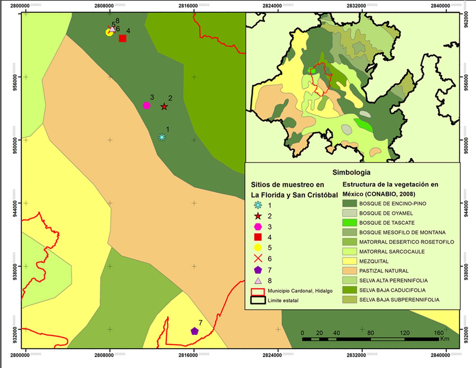
En total se tomaron muestras de 8 sitios, 4 en cada localidad. Para cada sitio se registraron las siguientes variables ambientales: exposición —determinada con una brújula —, pendiente del terreno —medida con un clinómetro Suunto— y altitud —registrada mediante una antena GPS Garmin eTrex 20x. Para determinar las condiciones edáficas, en cada sitio se recolectó una muestra de ~1 kg de suelo, previa remoción de la hojarasca superficial. Posteriormente, se realizaron las siguientes determinaciones: pH, materia orgánica (MO), nitrógeno inorgánico (N inorg.), fósforo asimilable (P), potasio (K), calcio (Ca), hierro (Fe), así como los porcentajes de limo, arena y arcilla, con los que se determinó la textura del suelo (TEX).
Para describir la estructura de la vegetación se utilizó el método de cuadrantes centrados en un punto utilizado por Granados-Victorino et al. (2015), método que no depende de un área delimitada y se basa en las distancias entre puntos fijos y los individuos más cercanos en cada cuadrante. En cada sitio se establecieron 10 puntos de muestreo, con una distancia de 20 m entre sí. En cada punto de muestreo se trazaron, de manera teórica, 4 cuadrantes a partir de ejes perpendiculares (en forma de plano cartesiano). En cada cuadrante se registró la distancia del punto central hasta el árbol o arbusto más cercano con una altura igual o mayor a un metro.
Los individuos registrados fueron identificados taxonómicamente, se midió su altura, con un flexómetro para aquellos individuos menores a 1.50 m y con un clinómetro para especies de porte mayor. Se estimó la cobertura de copa promediando 2 medidas de diámetro de la copa, tomadas en dirección norte-sur y este-oeste. Con los datos obtenidos y siguiendo la metodología propuesta por Cottam y Curtis (1956), modificada por Alanís-Rodríguez et al. (2020), se calcularon los valores relativos de abundancia, dominancia y frecuencia de las especies registradas. A partir de estos parámetros, se estimó el índice de valor de importancia relativa (VIR), el cual permite determinar la relevancia estructural de cada especie en la comunidad.
Con base en el VIR de cada especie, se realizó un análisis de agrupamiento utilizando el índice de disimilitud de Bray-Curtis como medida de distancia y el algoritmo de unión por promedio entre grupos (UPGMA). El índice de disimilitud de Bray-Curtis se utiliza para comparar la composición entre sitios e ignora los casos en los que las especies están ausentes, utiliza los valores del VIR (Rocha-Ramírez et al., 2013). A partir de un nivel de corte de 55% de la información retenida en el dendrograma, se identificaron los sitios con mayor semejanza estructural y se definieron las asociaciones vegetales dominantes.
La nomenclatura de las asociaciones vegetales se definió con base en las especies con mayor VIR en los grupos formados a partir del análisis de agrupamiento, así como la fisionomía general de las especies dominantes, de acuerdo con lo sugerido en González-Medrano (2004). Para representar gráficamente la estructura vertical y horizontal de estas asociaciones, se elaboró un perfil semirrealista de la vegetación del transecto de estudio, tomando como base los valores estructurales obtenidos. El análisis de ordenación se realizó mediante un análisis de correspondencias canónicas (ACC), que consiste en una regresión múltiple donde se relacionó el VIR de las especies con las variables ambientales y edáficas registradas. Ambos análisis se llevaron a cabo con el software Past v.4.03 (Hammer et al., 2001).
Resultados
Se identificaron 89 especies en las comunidades vegetales con presencia de Juniperus angosturana en el Valle del Mezquital, que pertenecen a 73 géneros y 41 familias. Las familias más representativas fueron Asteraceae con 10 especies, seguida de Cactaceae y Fabaceae con 8 especies cada una y Asparagaceae con 7. La localidad con mayor riqueza especifica fue La Florida con 72 especies.
Juniperus angosturana se desarrolla principalmente en matorrales, aunque también puede figurar como un elemento importante en los bosques de coníferas de las zonas semiáridas, en especial en aquellos dominados por pinos piñoneros y enebros (Juniperus spp.) (Romme et al., 2009). En las localidades del Valle del Mezquital se reconocieron 4 tipos de vegetación (tabla 1) y 4 asociaciones vegetales con presencia de J. angosturana, las cuales presentan diferencias estructurales y florísticas (figs. 2, 3). A continuación, se describen las características de cada una de dichas asociaciones: a) asociación Juniperus angosturana – Juniperus flaccida Scltdl. Esta asociación vegetal se encuentra en la localidad de San Cristóbal, en específico en los sitios 4 y 5, en altitudes que oscilan entre 1,970 y 2,070 m, con pendiente de 10 a 20% y exposición noroeste. Los suelos son pedregosos, con textura franco-arcillosa, moderadamente alcalinos, con bajo contenido de MO y altas concentraciones de Ca. La comunidad vegetal es codominada por Juniperus angosturana y Juniperus flaccida Schltdl., con VIR de 44% y 31%, respectivamente. Se trata de un bosque con baja densidad arbórea, en el que predominan los individuos de porte bajo que no sobrepasan 4 metros de altura, en cuyos claros es común la presencia de arbustos. Otras especies que se pueden encontrar son Agave lechuguilla Torr., Agave salmiana Otto ex Salm-Dyck var. salmiana, Berberis pallida Benth., Calliandra eriophylla Benth., Cercocarpus fothergilloides Kunth, Chrysactinia mexicana A. Gray, Cylindropuntia imbricata (Haw.) F.M. Knuth, Dalea bicolor Humb. et Bonpl. ex Willd., Dalea greggii A. Gray, Echinocactus platyacanthus Link et Otto, Ferocactus latispinus (Haw.) Britton et Rose, Flourensia resinosa (T. S. Brand.) Blake, Malacomeles denticulata (Kunth) Decne., Mammillaria sp., Milla biflora Cav., Opuntia rastrera F. A. C. Weber, Opuntia robusta H.L. Wendl. ex Pfeiff., Opuntia tomentosa Salm-Dyck, Perymenium mendezii DC., Sanvitalia procumbens Lam., Senna guatemalensis var. hidalgensis H. S. Irwin et Barneby, Thymophylla setifolia Lag., así como algunos individuos de Pinus cembroides Zucc, en las zonas más elevadas (fig. 4A). b) Asociación Juniperus angosturana – Pinus cembroides, se registró en los sitios 6 y 8 de San Cristóbal, entre 1,985 y 2,080 m snm, en pendientes de 10 a 30% y exposición noreste. Juniperus angosturana presentó el VIR más alto con 29%. El estrato arbóreo está compuesto por P. cembroides (21%), J. flaccida (5%) y Pinus pinceana Gordon et Glend (4.6%), conforman un dosel cuya altura varía entre 2 y 6 m. Además de J. angosturana, el estrato arbustivo incluye Ephedra compacta Rose, Rhus schiedeana Schltdl. y Rhus standleyi F.A. Barkley. Asimismo, se registraron especies como Agave lechuguilla, Agave salmiana var. salmiana, Chrysactinia mexicana, Electranthera mutica (DC.) Mesfin, D.J. Crawford et Pruski, Cylindropuntia imbricata, Dalea greggii, Flourensia resinosa, Milla biflora, Opuntia rastrera, Opuntia tomentosa, Perymenium mendezii, Sanvitalia procumbens, y Zinnia peruviana (L.) L. Este matorral se desarrolla sobre suelos pedregosos, con pH alcalino, de textura franco-arcillo-arenosa y con una elevada concentración de Ca y Fe (fig. 4B). c) Juniperus angosturana – Nolina parviflora. En esta asociación vegetal J. angosturana es la especie estructuralmente dominante, con un VIR de 57%. Coexiste con P. cembroides, Nolina parviflora (Kunth) Hemsl, J. flaccida, Dasylirion longissimum Lem., Agave salmiana Otto ex Salm-Dyck var. salmiana, Echinocactus platyacanthus Link et Otto, Ephedra compacta y diversas especies del género Opuntia. El estrato arbustivo no supera los 2 m de altura y en el estrato arbóreo los individuos más grandes llegan a medir hasta 5 m. Esta asociación, se distribuye en La Florida, específicamente en los sitios 1, 2 y 7, en altitudes que van de 1,800 a 2,050 m, en laderas con exposición sureste y pendientes de 7 a 30%. Los suelos son poco desarrollados, cuentan con una delgada capa de hojarasca y fragmentos sueltos de roca; presentan bajo contenido de materia orgánica (8%) y un pH de entre 7 y 8, y son ricos en Ca y K. Otras especies registradas fueron: Agave lechuguilla, Chrysactinia mexicana, Electranthera mutica, Cylindropuntia imbricata, Dahlia coccinea Cav., Dalea bicolor, Flourensia resinosa, Gochnatia hypoleuca (DC.) A. Gray, Lysiloma sp., Mammillaria sp., Milla biflora, Opuntia rastrera, Opuntia tomentosa, Perymenium mendezii DC., Sanvitalia procumbens, Sclerocarpus uniserialis, Thymophylla setifolia y Zinnia peruviana (fig. 4C). d) Juniperus angosturana – Neltuma laevigata, se registró únicamente en un sitio de muestreo, en La Florida, a una altitud promedio de 2,000 m, con una pendiente de 25% y exposición sureste. El suelo presenta una textura fina franco-arcillosa, y una alcalinidad ligera. Según los VIR, Juniperus angosturana es la especie dominante en el estrato arbustivo, con valor de 36% y alturas inferiores de 3 m. En el estrato arbóreo, con un dosel de entre 2 y 6 m de altura, destacan las especies Senegalia berlandieri Benth. y Neltuma laevigata (Humb. y Bonpl. ex Willd.) Britton y Rose,con un VIR conjunto de 25%. Asimismo, se registraron otras especies como Cylindropuntia imbricata, Cylindropuntia leptocaulis (DC.) F.M. Knuth, Milla biflora, Opuntia tomentosa, Jatropha dioica Sessé ex Cerv., Sclerocarpus uniserialis (Hook.) Benth. et Hook. f. ex Hemsl., Senna holwayana (Rose) I. et Barneby, Uncaria tomentosa (Willd. ex Schult.) DC. y Yucca filifera Chabaud (fig. 4D).
Tabla 1. Clasificación de la vegetación en las localidades La Florida y San Cristóbal en Cardonal, Hidalgo, basado en lo propuesto por González-Medrano (2004) para la vegetación de México.
| Categoría | Denominación |
| Tipo de vegetación | Bosque bajo de escuamifolios |
| Asociación | Juniperus angosturana – Juniperus flaccida |
| Tipo de vegetación | Bosque bajo de aciculifolios |
| Asociación | Juniperus angosturana – Pinus cembroides |
| Tipo de vegetación | Matorral mediano rosetófilo |
| Asociación | Juniperus – Nolina parviflora |
| Tipo de vegetación | Bosque bajo espinoso |
| Asociación | Juniperus angosturana – Neltuma laevigata |
Con base en los resultados obtenidos, las especies de mayor importancia ecológica en las asociaciones, además de J. angosturana, son P. cembroides, J. flaccida, Senegalia berlandieri,Neltuma laevigata y Nolina parviflora,las cuales presentaron los valores de importancia relativa más altos en las localidades muestreadas. La dominancia de Juniperus angosturana se atribuye principalmente a su mayor diámetro de copa, más que a su altura, en comparación con las demás especies representativas. La asociación más observada fue la de Pinus cembroides-Juniperus angosturana, seguida de J. angosturana-J. flaccida. Ambas asociaciones vegetales presentan acompañamiento de especies típicas de matorral xerófilo.
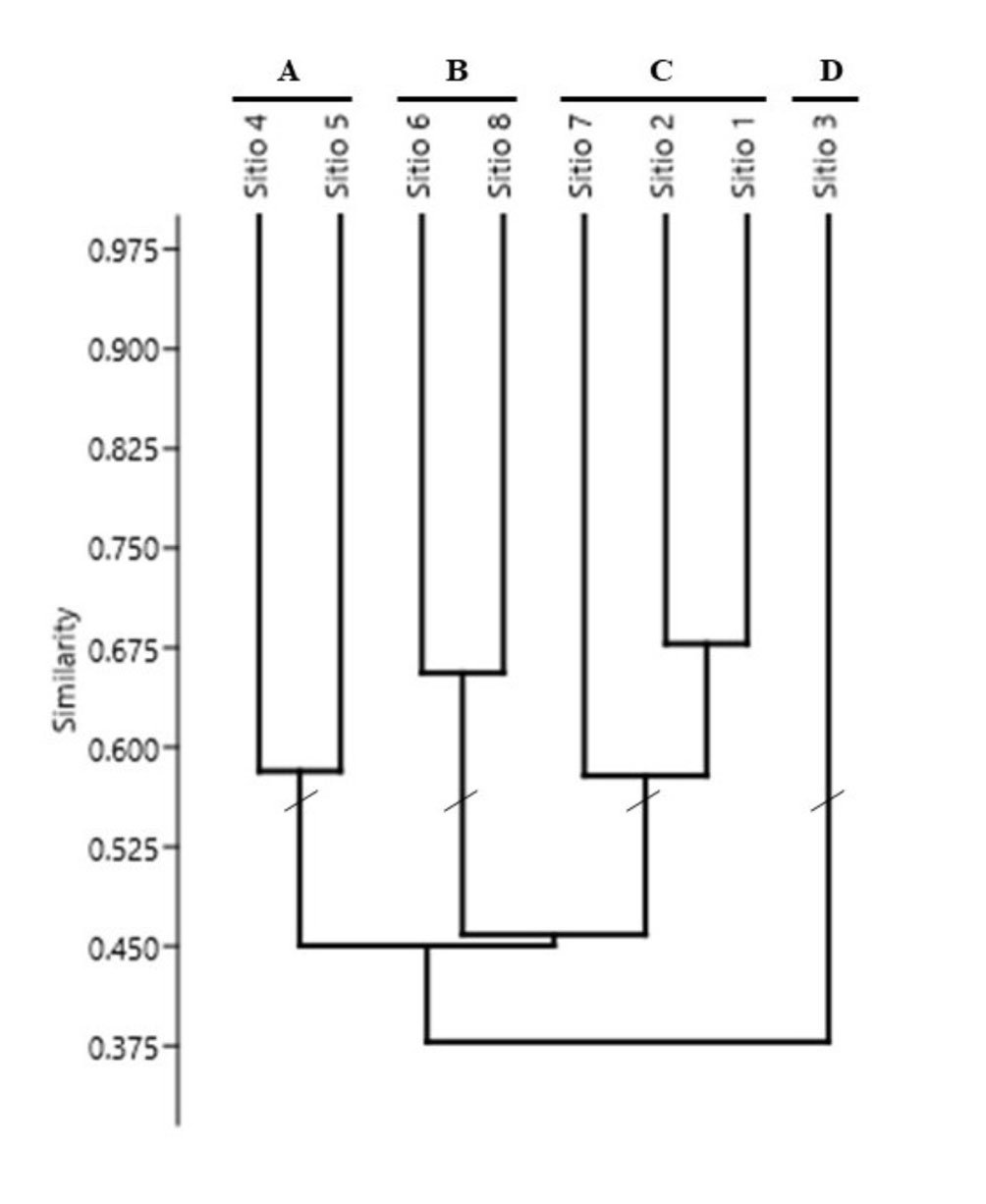
La diferenciación estructural de las asociaciones vegetales dominadas por Juniperus angosturana responde a un origen multifactorial y tiene una correlación, principalmente, con las variables edáficas (fig. 5). De acuerdo con el ACC, esta variación es explicada en 67.13% por los 3 primeros ejes (tablas 2, 3). Las variables edáficas más influyentes son la textura del suelo —en especial los porcentajes de arena y limo—, las concentraciones de Ca, K y P, así como el pH del suelo (tabla 2).
Discusión
Juniperus angosturana es una especie endémica de México, cuya distribución se extiende desde Coahuila hasta Hidalgo. A pesar de su relevancia estructural en las zonas áridas del país, ha sido escasamente estudiada desde una perspectiva ecológica. La mayoría de los trabajos publicados se han centrado en análisis filogenéticos (Adams, 1994; Adams y Schwarzbach, 2013; Uckele et al., 2021), en descripciones morfológicas y de distribución geográfica (Estrada-Castillón et al., 2014; Farjon, 2019; González-Elizondo et al., 2012), así como en modelos de distribución potencial o modelados de panbiología (Cartereau, et al., 2023; Morales-Garduño et al., 2021; Trájer, 2023).
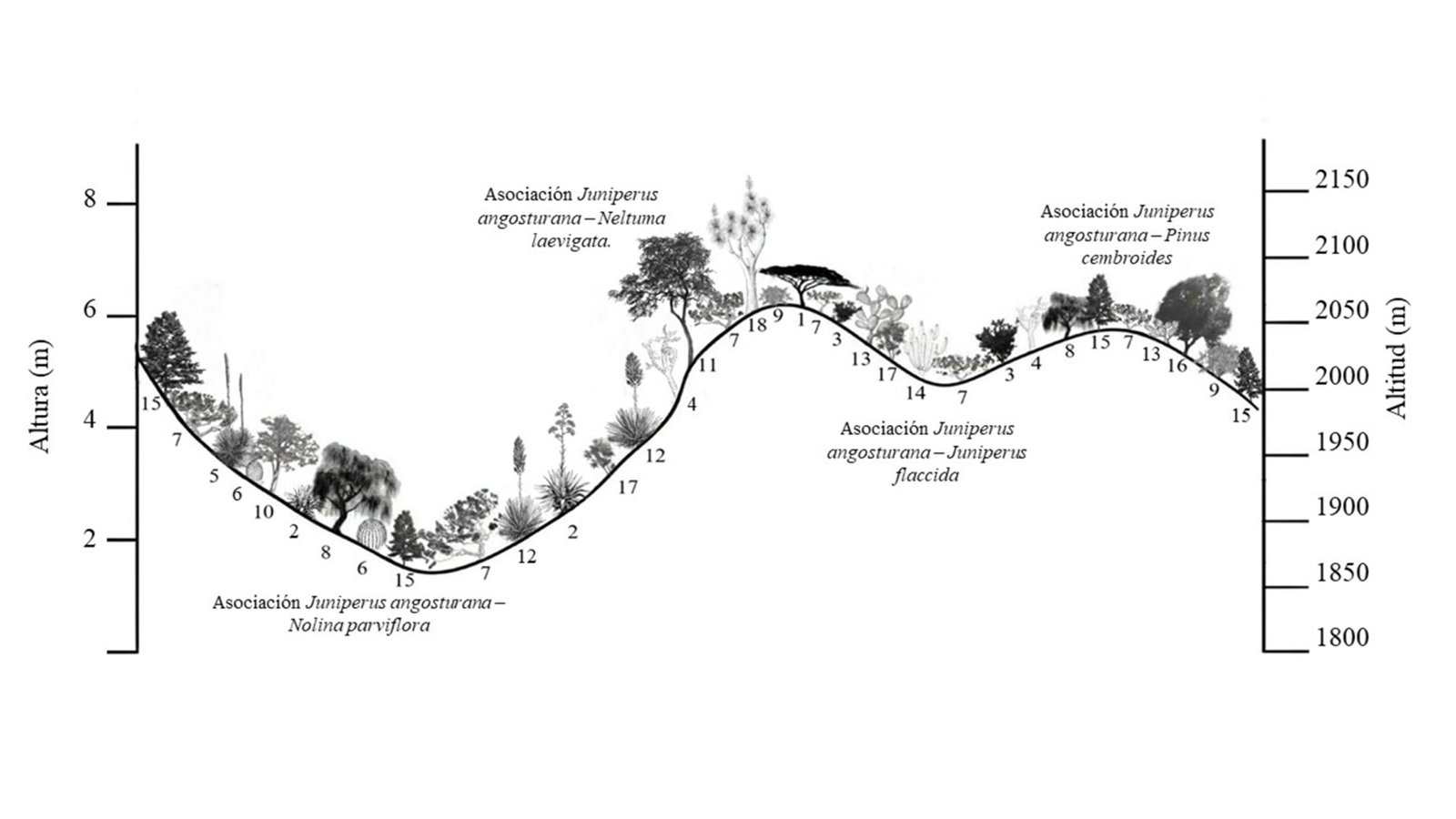
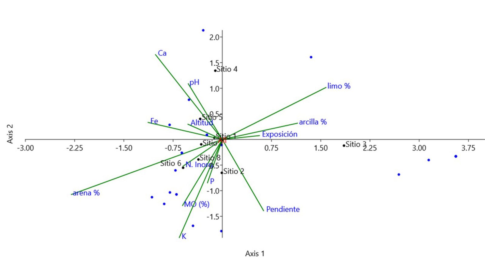
Tabla 2. Resultados de los primeros tres ejes de ordenación, de acuerdo con el análisis de correspondencias canónicas (ACC). Los valores en negritas señalan las variables con mayor peso en la definición de cada eje.
| Variable | Eje 1 | Eje 2 | Eje 3 |
| pH | -0.172893 | 0.36276 | 0.658303 |
| MO (%) | -0.202071 | -0.429806 | -0.215268 |
| N inorg. | -0.199503 | -0.173747 | 0.0472623 |
| P | -0.0753286 | -0.282118 | -0.700757 |
| K | -0.218424 | -0.638471 | -0.248518 |
| Ca | -0.339255 | 0.552029 | -0.00914643 |
| Fe | -0.377003 | 0.110919 | -0.443264 |
| arena (%) | -0.766368 | -0.357859 | 0.0899592 |
| limo (%) | 0.526614 | 0.338468 | 0.363971 |
| arcilla (%) | 0.381808 | 0.105922 | -0.377697 |
| Pendiente | 0.20969 | -0.463599 | 0.177899 |
| Exposición | 0.18856 | 0.0252954 | -0.295587 |
| Altitud | -0.174418 | 0.0991923 | -0.140028 |
| Distribución de la varianza | |||
| Valor propio | 0.521 | 0.364 | 0.318 |
| Varianza (%) | 29.07 | 20.3 | 17.76 |
| Varianza acumulada (%) | 29.07 | 49.37 | 67.13 |
Tabla 3. Matriz de correlación entre las variables ambientales y edáficas de los sitios de muestreo en Cardonal, Hidalgo. La parte superior derecha muestra los valores del coeficiente de correlación (r) y la diagonal inferior izquierda los valores de p (< 0.05)
| pH | MO (%) | N (inorgánico) | P | K | Ca | Fe | arena % | limo % | arcilla % | Pendiente | Exposición | |
| pH | -0.06 | -0.26 | -0.43 | -0.67 | -0.09 | -0.17 | -0.23 | -0.01 | 0.24 | -0.04 | -0.53 | |
| MO (%) | 0.85 | -0.56 | 0.75 | 0.56 | -0.06 | 0.57 | 0.3 | -0.69 | 0.24 | -0.07 | -0.58 | |
| N (Ing) | 0.39 | 0.05 | -0.55 | 0.11 | -0.12 | -0.12 | 0.27 | 0.37 | -0.56 | 0.04 | 0.22 | |
| P | 0.14 | 0.00 | 0.05 | 0.42 | -0.09 | 0.39 | 0.16 | -0.77 | 0.44 | 0.11 | -0.08 | |
| K | 0.01 | 0.05 | 0.72 | 0.15 | 0.21 | 0.48 | 0.63 | -0.22 | -0.48 | -0.14 | 0.01 | |
| Ca | 0.77 | 0.85 | 0.70 | 0.77 | 0.49 | 0.47 | 0.31 | 0.25 | -0.51 | -0.71 | 0.17 | |
| Fe | 0.58 | 0.04 | 0.70 | 0.19 | 0.10 | 0.11 | 0.21 | -0.24 | -0.04 | -0.77 | -0.40 | |
| arena % | 0.45 | 0.32 | 0.37 | 0.60 | 0.02 | 0.30 | 0.49 | -0.42 | -0.71 | -0.08 | -0.09 | |
| limo % | 0.97 | 0.01 | 0.21 | 0.00 | 0.47 | 0.41 | 0.43 | 0.15 | -0.34 | -0.29 | 0.31 | |
| arcilla % | 0.43 | 0.43 | 0.05 | 0.13 | 0.10 | 0.07 | 0.90 | 0.01 | 0.26 | 0.13 | -0.15 | |
| Pendiente | 0.90 | 0.82 | 0.90 | 0.72 | 0.65 | 0.01 | 0.002 | 0.80 | 0.34 | 0.67 | 0.08 | |
| Exposición | 0.06 | 0.04 | 0.47 | 0.80 | 0.97 | 0.58 | 0.18 | 0.77 | 0.30 | 0.62 | 0.80 | |
| Altitud | 0.23 | 0.21 | 0.00 | 0.07 | 0.32 | 0.80 | 0.82 | 0.70 | 0.02 | 0.02 | 0.60 | 0.95 |
En cuanto al hábitat de J. angosturana y las comunidades vegetales de las que forman parte, Estrada-Castillón et al. (2015) asocian la especie con ecotonos entre pastizales halófitos y bosques de pino piñonero en la región centro-sur de Nuevo León y el norte de Tamaulipas. De manera similar, Salinas-Rodríguez et al. (2013) reporta su presencia en el ecotono entre chaparrales de encino (Quercus spp.) y bosques de Pinus cembroides en el cañón de Iturbide, Nuevo León.
En Hidalgo, J. angosturana se desarrolla principalmente en la zona de transición entre el bosque de pino piñonero y el matorral rosetófilo. Lo anterior sugiere que es una especie ecotonal, con ventajas competitivas en los límites de la distribución de las asociaciones vegetales circundantes, es decir, en los márgenes de tolerancia física y competitiva de otras especies (Ortiz-Colín y Hulshof, 2024). Su relevancia estructural disminuye conforme se adentra en ecosistemas más homogéneos; sin embargo, se registraron matorrales dominados por J. angosturana, lo que indica una amplia tolerancia ecológica, tanto en términos edáficos como de humedad, temperatura y exposición solar. Esto refuerza su papel como especie clave en zonas de transición y como posible estabilizador ecológico en ambientes semiáridos.
Los matorrales dominados por J. angosturana forman un hábitat heterogéneo, que incluye microhábitats favorables bajo el dosel de los individuos, gracias a su amplia ramificación y extensión de copa. Esta estructura proporciona protección de la radiación solar y facilita la retención de suelo y humedad que beneficia a numerosas especies asociadas. No obstante, debido a los grandes volúmenes de enraizamiento de los arbustos, los espacios intermedios entre individuos suelen presentar escasa vegetación (Chambers et al., 1999; Rostamikia et al., 2024). Dicha configuración espacial da lugar a un mosaico ecológico conocido como islas de fertilidad o islas de recursos, que son esenciales para el mantenimiento de la biodiversidad en los ecosistemas áridos y semiáridos (Magaña et al., 2023).
En el Valle del Mezquital, la asociación más frecuente con presencia de Juniperus angosturana se presentó en los bosques de piñón-enebro, lo que evidencia una clara coexistencia con P. cembroides. No obstante, es necesario intensificar los estudios para confirmar si este patrón se mantiene en otras regiones. Romme et al. (2009) mencionan la presencia de 3 variantes para esta asociación: bosques persistentes de piñón-enebro, matorrales boscosos de piñón-enebro y sabanas de piñón-enebro, de los cuales solo los primeros 2 fueron registrados en el Valle del Mezquital, lo cual indica una alta variación estructural y ecológica.
En México, la asociación piñón-enebro se ha reportado en zonas de transición en regiones semiáridas. A pesar de su similitud estructural, existe una clara diferenciación florística regional y solo se había documentado la presencia de J. angosturana en Nuevo León, ahora se reporta también en Hidalgo. Por ejemplo, Parra-Álvarez et al. (2022) identificaron en la región central de San Luis Potosí, una asociación integrada por 5 especies de pinos piñoneros (Pinus cembroides, P. pinceana, P. nelsonii, P. discolor y P. johannis) y Juniperus flaccida. De forma similar, Granados-Victorino et al. (2015) reportaron esta asociación en la zona árida poblano-veracruzana, donde Pinus cembroides subsp. orizabensis D.K. Bailey codomina con J. flaccida o J. deppeana Steud; de la Fuente Solís et al. (2025) describen un bosque caracterizado por la asociación Pinus cembroides y Juniperus monosperma (Engelm.) Sarg. en Galeana, Nuevo León.
Baker y Shinneman (2004) señalan que estos bosques están aumentando en densidad y expandiéndose hacia los matorrales y pastizales adyacentes, los cuales frecuentemente se consideran ecosistemas en proceso de degradación. Se ha documentado que la remoción de individuos de Pinus o Juniperus puede favorecer el incremento de cobertura de gramíneas (Almalki et al., 2023), lo que representa un beneficio potencial para la ganadería. Sin embargo, esta práctica tiene efectos negativos en la biodiversidad debido a que los árboles y arbustos de las zonas áridas y semiáridas proporcionan sitios seguros de germinación, así como refugio y hábitat para numerosas especies (Allegrezza et al., 2016).
Por medio del ACC se determinó que la textura del suelo, en particular los porcentajes de arena y limo, constituye uno de los principales factores que explican la diferenciación estructural entre la vegetación de los sitios analizados. La proporción relativa de arena, limo y arcilla influye directamente en la fertilidad del suelo, pues regula la retención de humedad y la disponibilidad de nutrientes esenciales para las plantas. Los suelos con textura arenoso-limosa, al presentar baja capacidad de retención de agua y de intercambio catiónico, favorecen el desarrollo de especies adaptadas a ambientes con pulsos breves de humedad (Rostamikia et al., 2024). Por lo tanto, el gradiente de textura puede inducir un recambio en la composición vegetal, puesto que refleja la capacidad diferencial de las especies para tolerar condiciones edáficas restrictivas.
Las variaciones en la textura podrían deberse a la erosión eólica e hídrica provocadas por las diferencias en la exposición, la pendiente y la abundancia de las especies vegetales (Shukla et al., 2006). Por ejemplo, en el desierto chihuahuense, las diferencias estructurales en las asociaciones vegetales se presentan debido a los ligeros cambios en la orografía, la elevación, el ángulo de la pendiente, la rocosidad y las variables edáficas en la distribución de las plantas en ambientes áridos (Estrada-Castillón et al., 2015; Granados-Sánchez et al., 2011).
En el Valle del Mezquital, las asociaciones vegetales dominadas por especies del género Juniperus, como los bosques de enebro y los matorrales submontanos de Juniperus angosturana, se desarrollan sobre suelos de origen calcáreo, con pH alcalino y altos contenidos de Fe, características típicas de zonas áridas donde la escasez de agua limita los procesos de lixiviación, además de generar la formación de costras de carbonatos o de yesos (Hag Husein et al., 2021). Diversas especies del género Juniperus han sido reconocidas por su notable capacidad de adaptación a suelos pobres en nutrientes, poco profundos y con baja retención de humedad. Además, presentan una respuesta eficiente ante cambios ambientales, así como una alta tolerancia al fuego y a perturbaciones de origen antrópico (Cuevas-Guzmán et al., 2023; Rosas-Chavoya et al., 2016).
De forma general, las variantes estructurales de las comunidades dominadas por J. angosturana está influenciada por la textura del suelo, la disponibilidad de nutrientes y el pH, que suele ser alcalino y en menor medida, la pendiente del terreno. Por ejemplo, la asociación Juniperus angosturana-Pinus cembroides se desarrolla en suelos poco profundos con alto contenido de arena, pH ligeramente alcalino y mayor contenido de materia orgánica y, por ende, una mayor disponibilidad de nutrientes respecto a las demás asociaciones analizadas. En contraste, la asociación de matorral de Juniperus angosturana–Nolina parviflora se presentan en suelos con texturas más finas, que retienen mejor el agua superficial, sin embargo, muestran baja acumulación de materia orgánica y mayor exposición solar, lo que genera condiciones edáficas más restrictivas para el desarrollo arbóreo.
El presente estudio representa una contribución significativa al conocimiento ecológico de J. angosturana al proporcionar información básica sobre su hábitat y las asociaciones vegetales que conforma. Los resultados confirman que es una especie ecotonal, cuya plasticidad ambiental le permite establecerse y adaptarse a condiciones edáficas y climáticas variables en zonas de transición entre bosques de pino piñonero y matorral rosetófilo. La presencia de J. angosturana en Hidalgo, relativamente lejos de su distribución previamente conocida, amplía el conocimiento sobre su rango ecológico y florístico, y subraya la necesidad de llevar a cabo más estudios regionales, con un enfoque en la restauración de dichos ecotonos.
Además, su hábito de crecimiento y cobertura favorecen la generación de islas de fertilidad, promueven la biodiversidad y contribuyen a la conectividad del paisaje al conformar corredores biológicos, que facilitan el flujo de especies entre ecosistemas fragmentados. La identificación de su preferencia por suelos de textura arenoso-limosa y de origen calcáreo, así como de la coocurrencia con P. cembroides en el Valle del Mezquital, aporta elementos clave para comprender la dinámica y la diferenciación florística de los ecosistemas áridos y semiáridos donde se desarrolla J. angosturana.
En conjunto, los resultados obtenidos en este trabajo constituyen una base técnica y ecológica sólida para orientar estrategias de conservación y manejo de matorrales donde J. angosturana actúa como especie estructuralmente dominante. La identificación de los factores edáficos y ambientales que determinan su distribución, así como el reconocimiento de las especies vegetales que la acompaña, proporcionan información fundamental para el diseño de acciones de restauración ecológica y el manejo adaptativo de los ecosistemas semiáridos donde esta especie se desarrolla.
Agradecimientos
Los autores agradecen a la Universidad Autónoma Chapingo, en particular a la Dirección General de Investigación, Posgrado y Servicio y a la División de Ciencias Forestales, por las facilidades y el apoyo institucional brindados para la realización de esta investigación; a la Secretaría de Ciencia, Humanidades, Tecnología e Innovación (Secihti) por la beca de posgrado número 4008144 otorgada a la primera autora durante el desarrollo de estos estudios. A los compañeros, Diego Carrillo Martínez, Ruth del Cid, así como al técnico Rubén Herrera Flores por su apoyo en el trabajo de campo y a Ana Rosa López Ferrari por su apoyo en la identificación taxonómica de algunos ejemplares en el Herbario UAMIZ. Finalmente, se agradecen las valiosas sugerencias y observaciones de los revisores, que contribuyeron significativamente a mejorar el contenido de este escrito.
Referencias
Adams, R. P. (1994). Geographic variation and systematics of monospermous Juniperus (Cupressaceae) from the Chihuahua Desert based on RAPD’s and terpenes. Biochemical Systematics Ecology, 22, 699–710. https://doi.org/10.1016/03051978(94)90056-6
Adams, R. P. y Schwarzbach, A. E. (2013). Taxonomy of the serrate leaf Juniperus of North America: phylogenetic analyses using nrDNA and four cpDNA regions. Phytologia, 95, 172–178.
Alanis-Rodríguez, E., Mora-Olivo, A. y Marroquín-de la Fuente, J. (2020). Muestreo ecológico de la vegetación. Monterrey, México: Universidad Autónoma de Nuevo León.
Allegrezza, M., Corti, G., Cocco, S., Pesaresi, S., Chirico, G. B., Saracino, A. et al. (2016). Microclimate buffering and fertility island formation during Juniperus communis ontogenesis modulate competition-facilitation balance. Journal of Vegetation Science, 27, 616–627. https://doi.org/10.1111/jvs.12386
Almalki, Y. M., Fernald, A. G., Ochoa, C. G., Cibils, A. F., Faist, A. M., Cram, D. S. et al. (2023). Understory vegetation response to thinning pinyon-juniper woodlands. Rangeland Ecology & Management, 88, 152–158. https://doi.org/10.1016/j.rama.2023.02.012
Baker, W. L. y Shinneman, D. J. (2004). Fire and restoration of piñon-juniper woodlands in the western United States. Forest Ecology and Management, 189, 1–21. https://doi.org/10.1016/j.foreco.2003.09.006
Cartereau, M., Leriche, A., Médail, F. y Baumel, A. (2023). Tree biodiversity of warm drylands is likely to decline in a drier world. Global Change Biology, 29, 3707–3722. https://doi.org/10.1111/gcb.16722
Chambers, J. C., Vander Wall, S. B. y Schupp, E. W. (1999). Ecología de semillas y plántulas de especies de piñón y enebro en los bosques pigmeos del oeste de Norteamérica. Botanical Review, 65, 1–38. https://doi.org/10.1007/BF02856556
Cottam, G. y Curtis, J. T. (1956). The use of distance measurements in phytosociological sampling. Ecology, 37, 451–460. https://doi.org/10.2307/1930167
Cuevas-Guzmán, R., Canales-Piña, S., Sánchez-Rodríguez, E. V., Morales-Arias, J., Guzmán-Hernández, L. y Núñez-López, N. M. (2023). Atributos estructurales y hábitat de Juniperus jaliscana en Talpa de Allende, Jalisco, México. Botanical Sciences, 101, 670–684. https://doi.org/10.17129/botsci.3235
EncicloVida. (s. f.). Enebro chino. EncicloVida. Recuperado el 16 abril, 2024 de: https://enciclovida.mx/especies/155214
Estrada-Castillón E., Arévalo, J. R., Villarreal-Quintanilla, J. Á., Salinas-Rodríguez, M. M., Cantú-Ayala, C. M., González-Rodríguez, H. et al. (2014). Coníferas de Nuevo León, México. Nuevo León, México: Universidad Autónoma de Nuevo León.
Estrada-Castillón E., Arévalo, J. R., Villarreal-Quintanilla, J. Á., Salinas-Rodríguez, M. M., Encina-Domínguez, J. A., González-Rodríguez, H. et al. (2015). Classification and ordination of main plant communities along an altitudinal gradient in the arid and temperate climates of northeastern Mexico. The Science of Nature, 102, 9–10. https://doi.org/10.1007/s00114-015-1306-3
Farjon, A. (2019). Juniperus angosturana. Threatened Conifers of the World. https://threatenedconifers.rbge.org.uk/conifers/juniperus-angosturana
Fonseca, R. M. (2006). Juniperus, la ginebra, el incienso, los lápices y los repelentes. Ciencias, 81, 44–47.
Fuente-Solís, A. M., Alanís-Rodríguez, E., Yáñez-Díaz, M. I., Córdova-Silva, I., Himmelsbach, W. y Martínez del Campo-Delgado, Á. M. (2025). Analysis of the natural regeneration of a temperate arid forest in northeastern Mexico. Revista Forestal Mesoamericana Kurú, 22, 1–10. https://doi.org/10.18845/rfmk.v22i50.7755
GBIF Secretariat.(2023). Juniperus angosturana R. P. Adams. GBIF Backbone Taxonomy. https://doi.org/10.15468/39omei
González-Elizondo, M. S., González-Elizondo, M., Tena-Flores, J. A., Ruacho-González, L. y López-Enríquez, I. (2012). Vegetación de la sierra Madre Occidental, México: una síntesis. Acta Botanica Mexicana, 100, 351–403. https://doi.org/10.21829/abm100.2012.40
González-Medrano, F. (2004). Las comunidades vegetales de México. Propuesta para la unificación de la clasificación y nomenclatura de la vegetación de México, 2ª ed. México D.F.: Instituto Nacional de Ecología, Semarnat. https://www.academia.edu/16702033/Vegetacion_de_mexico_gonzalez
González-Medrano, F. (2012). Las zonas áridas y semiáridas de México y su vegetación. México D.F.: Instituto Nacional de Ecología, Semarnat. http://140.84.163.2:8080/xmlui/bitstream/handle/publicaciones/218/668_2012_Zonas_aridas_semiaridas_Mexico.pdf?sequence=1etisAllowed=y
Granados-Sánchez, D., Sánchez-González, A., Granados-Victorino, R. L. y Borja-de la Rosa, A. (2011). Ecología de la vegetación del desierto chihuahuense. Revista Chapingo Serie Ciencias Forestales y del Ambiente, 17, 111–130. https://doi.org/10.5154/r.rchscfa.2010.10.102
Granados-Victorino, R. L., Granados-Sánchez, D. y Sánchez-González, A. (2015). Caracterización y ordenación de los bosques de pino piñonero (Pinus cembroides subsp. orizabensis) de la cuenca oriental (Puebla, Tlaxcala y Veracruz). Madera y Bosques, 21, 23–42. https://doi.org/10.21829/myb.2015.212443
Guzmán-Cornejo, L., Sánchez Morales, A. y Pacheco, L. (2015). Helechos y licofitas del municipio de Cardonal, Hidalgo, México. Revista Mexicana de Biodiversidad, 86, 573–581. https://doi.org/10.1016/j.rmb.2015.06.004
Hag Husein, H., Lucke, B., Bäumler, R. y Sahwan, W. A. (2021). Contribution to soil fertility assessment for arid and semi-arid lands. Soil Systems, 5, 1–13. https://doi.org/10.3390/soilsystems5030042
Hammer, O., Harper, D. y Ryan, P. (2001). PAST: Paleontological Statistics Software Package for Education and Data Analysis. Paleontología Electrónica, 4, 1–9. https://www.researchgate.net/publication/259640226_PAST_Paleontological_Statistics_Software_Package_for_Education_and_Data_Analysis
Hernández-Armas, C. (2016). Otomíes del Valle del Mezquital: retos ante la preservación o la transformación de una cul-
tura. Divulgare. Boletín Científico de la Escuela Superior de Actopan, 3. https://doi.org/10.29057/esa.v3i5.1645
Hernández-González, D. E., Muñoz Iniestra, D. J., López Galindo, F. y Hernández Moreno, M. M. (2018). Impacto del uso de la tierra en la calidad del suelo en una zona semiárida del Valle del Mezquital, Hidalgo, México. BIOCYT Biología Ciencia y Tecnología, 11, 792–807. https://doi.org/10.22201/fesi.20072082.2018.11.65833
Herrerías, M. L. G. y Nieto, P. P. (2020). Características estructurales y demográficas de Juniperus deppeana Steud. en 2 localidades del estado de Tlaxcala. Revista Mexicana de Ciencias Forestales, 11, 124–151. https://doi.org/10.29298/rmcf.v11i61.618
IPNI (International Plant Names Index). (2025). The Royal Botanic Gardens, Kew, Harvard University Herbaria et Libraries y Australian National Herbarium. Recuperado el 24 Febrero, 2025 de: http://www.ipni.org
Natusfera. (s. f.). Enebro chino(Juniperus angosturana). Natusfera. Recuperado el 16 abril, 2024 de: https://spain.inaturalist.org/taxa/135936-Juniperus-angosturana
Magaña Ugarte, R., Gavilan, R. G. y Rubio, A. (2023). Assessing the occurrence of soil improvement and its relationship to the dominant life form in the high mountains of Central Spain. Geoderma Regional, 36, 1–11. https://doi.org/10.1016/j.geodrs.2023.e00744
Miwa, C. T. y Reuter, R. J. (2010). Persistence of western juniper (Juniperus occidentalis) resource islands following canopy removal. Northwest Science, 84, 361–368. https://doi.org/10.3955/046.084.0405
Morales-Garduño, L., Solano, E., Villaseñor, J. L. y Montaño-Arias, G. (2021). Panbiogeografía de los matorrales de la región xerofítica mexicana. Botanical Sciences, 99, 611–627. https://doi.org/10.17129/botsci.2773
Ortiz-Colin, P. y Hulshof, C. (2024). Ecotones as windows into organismal-to-biome scale responses across neotropical forests. Plants, 13, 2396. https://doi.org/10.3390/plants13172396
Parra-Álvarez, J., Granados-Sánchez, D., Granados-Victorino, R. L. y Villanueva-Morales, A. (2022). Caracterización estructural y clasificación de los bosques piñoneros de San Luis Potosí, México. Revista Chapingo Serie Ciencias Forestales y del Ambiente, 29, 61–98. https://doi.org/10.5154/r.rchscfa.2022.03.021
Pérez-Aguilar, L. Y., Plata-Rocha, W., Monjardín-Armenta, S. A., Franco-Ochoa, C. y Zambrano-Medina, Y. G. (2021). The identification and classification of arid zones through multicriteria evaluation and geographic information systems —case study: arid regions of northwest Mexico. ISPRS. International Journal of Geo-information, 10, 720. https://doi.org/10.3390/ijgi10110720
Portal de Geoinformación. (2023). Carta fisonómica-estructural de la vegetación de México. Comisión Nacional para el Conocimiento y Uso de la Biodiversidad Recuperado el 27 enero, 2025 de: http://www.conabio.gob.mx/informacion/gis/?vns=gis_root/usv/otras/vpotbt4mgw
Richards, P. (1952). The tropical rain forest an ecological study. Cambridge: Cambridge University Press.
Rocha-Ramírez, A., Chávez-López, R., Ramírez-Rojas, A. y Cházaro-Olvera, S. (2013). Comunidades. Métodos de estudios. México D.F.: Facultad de Estudios Superiores Iztacala, Universidad Nacional Autónoma de México.
Romme, W. H., Allen, C. D., Bailey, J. D., Baker, W. L., Bestelmeyer, B. T., Brown, P. M. et al. (2009). Historical and modern disturbance regimes, stand structures, and landscape dynamics in piñon-juniper vegetation of the western United States. Rangeland Ecology and Management, 62, 203–222. https://doi.org/10.2111/08-188R1
Romo, A., Salvá, C. M., Ouhammou, A. y Boratyński, A. (2012). Las formaciones de Sabina albar (Juniperus thurifera subsp. africana) en los macizos de Toubkal y Azourki del gran Atlas (Marruecos). VII Congreso Español de Biogeografía, 379-383. https://digital.csic.es/bitstream/10261/64701/1/formaciones_sabina_albar.pdf
Rosas-Chavoya, M., Granados-Sánchez, D., Granados-Victorino, R. L. y Esparza-Govea, S. (2016). Clasificación y ordenación de bosques de pino piñonero del estado de Querétaro. Revista Mexicana de Ciencias Forestales, 7, 52–73. https://doi.org/10.29298/rmcf.v7i33.90
Rostamikia, Y., Matinizadeh, M. y Anbaran S. M. (2024). Influence of scattered greek juniper trees on soil properties in semi-arid woodlands in the northwest of Iran. Journal of Forest Science, 70, 560–573. https://doi.org/10.17221/60/2024-jfs
Rzedowski, J. (2006). Vegetación de México. Comisión Nacional para el Conocimiento y Uso de la Biodiversidad. -https://www.biodiversidad.gob.mx/ecosistemas/vegetaciondeMexico
Salinas-Rodríguez, M. M., Estrada-Castillón, E. y Villarreal-Quintanilla, J. Á. (2013). Flora and phytogeography of the Cañón de Iturbide, Nuevo León, México. Journal of the Botanical Research Institute of Texas, 7, 803–819.
Shukla, M. K., Lal, R., Ebinger, M. y Meyer, C. (2006). Physical and chemical properties of soils under some piñon-juniper-oak canopies in a semi-arid ecosystem in New Mexico. Journal of Arid Environments, 66, 673–685. https://doi.org/10.1016/j.jaridenv.2005.12.002
Trájer, A. J. (2023). Clarification of the Lopingian palaeo climatic conditions of the northwestern coastal regions of Palaeotethys based on the transdanubian geological record. Review of Palaeobotany and Palynology, 316, 104917. https://doi.org/10.1016/j.revpalbo.2023.104917
Uckele, K. A., Adams, R. P., Schwarzbach, A. E. y Parchman, T. L. (2021). Genome-wide RAD sequencing resolves the evolutionary history of serrate leaf Juniperus and reveals discordance with chloroplast phylogeny. Molecular Phylogenetics and Evolution, 156, 107022. https://doi.org/10.1016/j.ympev.2020.107022
Villanueva-Díaz, J., Vázquez-Selem, L., Gómez-Guerrero, A., Cerano-Paredes, J., Aguirre-González, N. A. y Franco-Ramos, O. (2016). Potencial dendrocronológico de Juniperus monticola Martínez en el monte Tláloc, México. Revista Fitotecnia Mexicana, 39, 175–185. https://doi.org/10.35196/rfm.2016.2

Community structure of Thomisidae (Araneae, Araneomorphae) in Tepoztlán, Morelos, Mexico: a one-year seasonal study
Estructura de la comunidad de Thomisidae (Araneae, Araneomorphae) en Tepoztlán, Morelos, México: estudio estacional de un año
Fernando Pilo-García a, Víctor H. Toledo-Hernández b, *, Alejandro Valdez-Mondragón c
a Universidad Autónoma del Estado de Morelos, Facultad de Ciencias Biológicas, Av. Universidad 1001, Colonia Chamilpa, 62209 Cuernavaca, Morelos, Mexico
b Universidad Autónoma del Estado de Morelos, Centro de Investigación en Biodiversidad y Conservación, Av. Universidad 1001, Colonia Chamilpa, 62209 Cuernavaca, Morelos, Mexico
c Consejo Nacional de Humanidades, Ciencias y Tecnologías (CONAHCYT), Laboratorio de Aracnología, Centro Tlaxcala de Biología de la Conducta (CTBC), Universidad Autónoma de Tlaxcala, Mexico
*Corresponding author: victor.toledo@uaem.mx (V.H. Toledo-Hernández)
Received: 20 August 2025; accepted: 12 February 2026
Abstract
Spiders of the family Thomisidae are scarcely studied in Mexico, and ecological data for this family are practically nonexistent. To fill this gap, we carried out an ecological study of crab spiders in a deciduous tropical forest in San Andrés de la Cal, Tepoztlán, Morelos, central Mexico, evaluating seasonal variation in community structure over the annual cycle. Fieldwork consisted of systematized monthly diurnal collections by 5 people, implementing 3 sampling techniques: beating sheets, sweeping nets, and looking down. In total, we collected 839 spiders representing 9 genera and 16 species, of which 5 genera and 7 species are new state records. The highest richness, abundance, and diversity were recorded in the rainy season; however, unique species were found during each season. According to richness estimators, between 12 and 22% of the estimated species remain to be found in the study area. Evenness factors indicated that the community is composed primarily of rare species, with only a few dominant species. While this study reports a reliable inventory for the region, the species accumulation curve did not reach the asymptote, suggesting that additional ecological studies employing diverse protocols are needed to complement our knowledge of these spiders.
Keywords: Crab spiders; Deciduous tropical forest; Ecology; Diversity; Seasonality
Resumen
En México, la familia Thomisidae está poco estudiada y los datos ecológicos son prácticamente inexistentes. Para subsanar esta deficiencia, realizamos un estudio ecológico de arañas cangrejo en un bosque tropical caducifolio en San Andrés de la Cal, Tepoztlán, Morelos, centro de México, evaluando la variación estacional en la estructura de la comunidad durante un ciclo anual. El trabajo de campo consistió en colectas diurnas mensuales sistematizadas por 5 personas, implementando 3 técnicas de muestreo: paraguas entomológico, red entomológica y búsqueda directa. En total, recolectamos 839 individuos pertenecientes a 9 géneros y 16 especies, de los cuales 5 géneros y 7 especies son nuevos registros estatales. La mayor riqueza, abundancia y diversidad se registraron durante la temporada de lluvias; sin embargo, se registraron especies únicas en cada temporada. Según los estimadores de riqueza, faltan por registrarse en el área de estudio entre 12 y 22% de las especies estimadas. Los factores de uniformidad indicaron que la comunidad está compuesta principalmente por especies raras y pocas especies dominantes. El inventario obtenido es confiable; no obstante, la curva de acumulación no alcanzó la asíntota, sugiriendo la necesidad de realizar estudios ecológicos adicionales empleando diversos protocolos para complementar nuestro conocimiento de estas arañas.
Palabras clave: Arañas cangrejo; Selva baja caducifolia; Ecología; Diversidad; Estacionalidad
Introduction
In general, most studies on spider communities in Mexico have analyzed spatial diversity patterns, with fewer studies focusing on seasonal diversity and abundance (Campuzano & Padilla-Ramírez, 2020; Corcuera et al., 2019; Jiménez et al., 2020, 2024; Menéndez-Acuña et al., 2023; Pérez-Hernández & Zaragoza-Caballero, 2016; Rodríguez-Rodríguez et al., 2015). The study of seasonal diversity variation and its associated processes is crucial for understanding ecosystem dynamics and establishing effective conservation strategies. Moreover, understanding higher-taxon diversity can serve as a useful indicator of overall biodiversity (Williams & Gaston, 1994). Basic ecological information is lacking for many megadiverse biological groups, including spiders (Colwell & Coddington, 1994). In Mexico, 2,345 spider species have been recorded, comprising 455 genera and 70 families (Ponce-Saavedra et al., 2023). Despite this high diversity, only 2 country-level inventories of Mexican spiders have been compiled (Hoffmann, 1976; Jiménez, 1996), and it has been estimated that only ~ 23% of the country’s spider species are known (Francke, 2014; Ponce-Saavedra et al., 2023). Spiders are suitable model organisms for ecological studies due to the ease of obtaining large samples for statistical analyses, their limited dispersal capacity, their presence in almost every ecosystem, and their high abundance (Colwell & Coddington, 1994; Halaj et al., 1998; Jiménez-Valverde & Hortal, 2003; Turnbull, 1973). However, when generating a species inventory for a megadiverse group, encountering every species present at a certain locality takes considerable effort due to the existence of rare species, the wide variety of collecting techniques needed, and the difficulty to systematize sampling protocols (Gotelli & Cowell, 2011; Wolda, 1988). Therefore, it is often beneficial to focus sampling efforts on smaller taxonomic groups (families, subfamilies, tribes), facilitating the standardization of protocols and the increased capacity to detect a higher proportion of the overall species number (Jiménez-Valverde & Lobo, 2004, 2005, 2007). Crab spiders are an abundant and diverse group, one of the dominant spider families in the community. They are an important link in trophic chains as both predators and prey, and due to their proximity to the vegetation, these spiders are susceptible to changes in the environment (Benjamin, 2011; Benjamin et al., 2008; Clausen, 1986; Jocqué & Dippenaar-Schoeman, 2006; Lapp & Dondale, 2017; Morse, 2007). In addition, they are easy to identify in the field, making them a useful model for ecological studies and reliable regional faunistic inventories. In the Mexican state of Morelos, the first record of the family Thomisidae was made by F. O. Pickard-Cambridge (1895), who described Synema madidum from Cuernavaca. In the 128 years since then, only 5 species have been reported in 7 scientific papers (Pickard-Cambridge, 1895, 1900; Gertsch, 1953; Gertsch & Davis, 1940; Hoffmann, 1976; Nieto-Castañeda et al., 2014; Pickard-Cambridge, 1896). Similarly, ecological data for the family has been reported in only a few studies, which mostly focus on higher taxonomic levels (Hernández-Silva, 2016; Menéndez-Acuña, 2017; Nieto-Castañeda et al., 2014; Rivas-Herrera, 2015). To gather basic ecological data and initiate faunistic inventories for the family Thomisidae, we analyzed the community structure of crab spiders throughout an annual cycle. By comparing community structure across the rainy and dry seasons in a deciduous tropical forest, we aim to uncover temporal patterns in thomisid diversity and to contribute to the faunistic knowledge of these spiders in Morelos and Mexico more broadly.
Materials and methods
The study was carried out in the surroundings of San Andrés de la Cal, Tepoztlán, Morelos, in central Mexico (Fig. 1). The study area pertains to the protected areas Corredor Biológico Chichinautzin and Parque Nacional El Tepozteco (Conanp, 1983; INEGI, 2017), located at 18°56’11” N, 99°06’46” W, with an average altitude of 1,507 m asl (Fig. 1). The climate is characterized as (A) Cw2 (W) ig, warm subhumid, with summer rains (García, 2004). The mean annual temperature is 20.5 °C, and the mean annual precipitation is 1,091.8 mm (INEGI, 2017; Ruiz-Rivera, 2001). The dominant primary vegetation is deciduous tropical forest, characterized by trees under 12 meters in height and 2 marked seasons, a rainy season (June to October) and a dry season (November to May) (Balvanera & Maass, 2010; Miranda & Hernández, 1963; Trejo, 2010). Two study sites were selected: “Derrame de Lava” (DL), at 18°56’33.5” N, 99°06’57.4” W, and “Cerro de la Cal” (CC), at 18°56’38” N, 99°06’31” W (Fig. 1). Both sites have specific geomorphological characteristics that generate differences in the composition of woody plants. Sixty species of woody plants are known across both sites. In DL, 24 species are reported only for this site, with Sapium macrocarpum Müll. Arg. (Euphorbiaceae), Ipomea pauciflora M. Martens & Galeotti (Convolvulaceae), and Quercus obtusata Bonpl. (Fagaceae) predominant. In CC, 8 species were observed only at this site, with S. macrocarpum, Bursera fagaroides (Kunth) Engl., B. glabrifolia (Kunth) Engl., and B. copallifera (DC.) Bullock (Burseraceae) predominant (Vergara-Torres et al., 2010).
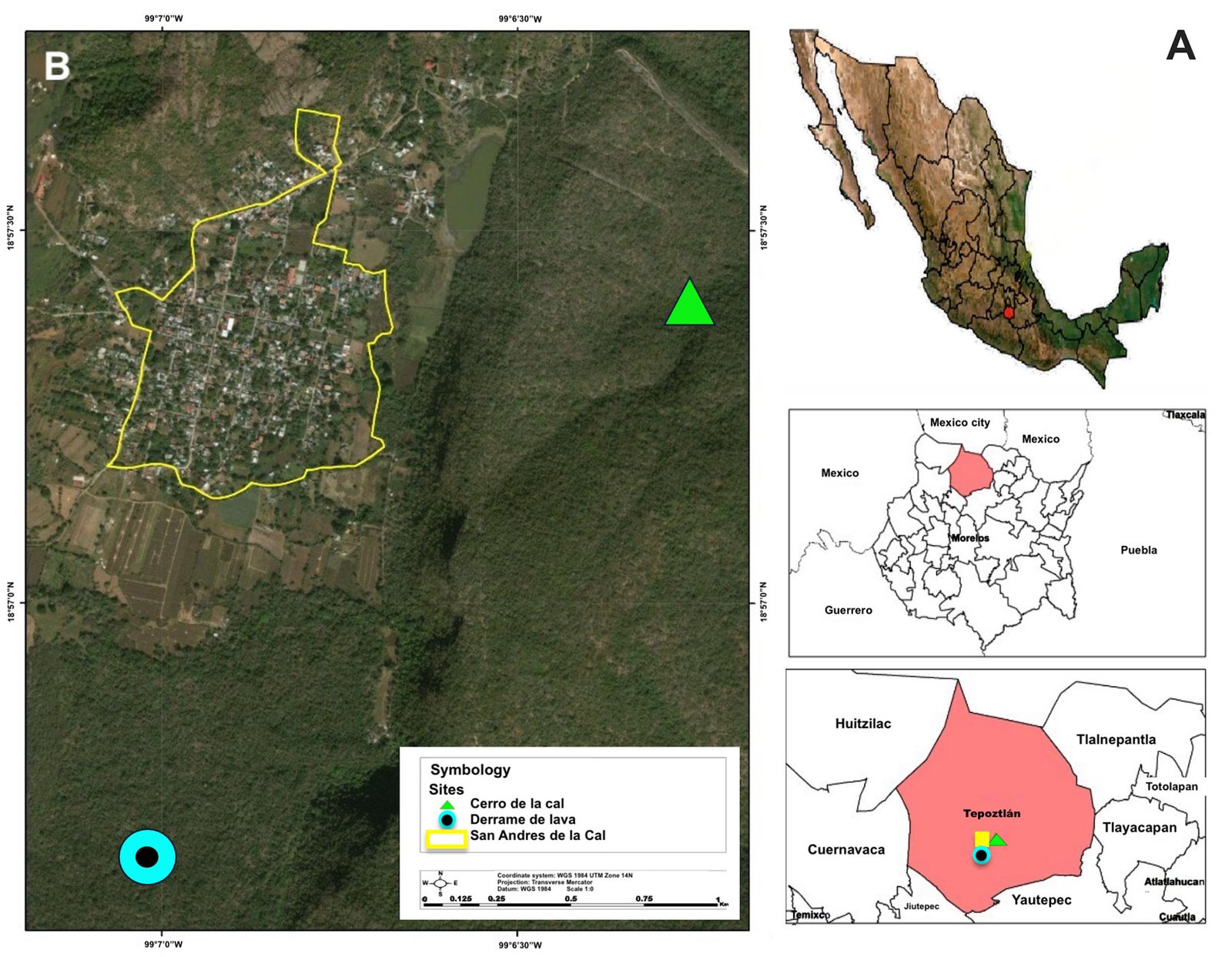
Spiders of the family Thomisidae were collected over a one-year period, from September 2017 to August 2018. A systematic collection protocol was implemented, involving 2 days per month at each site and 5 collectors. Because these spiders are diurnal, collections were made over 6 daylight hours per day, from 10:00 to 16:00 h (Abraham, 1983), with an effort of 6 hours per person. We applied 3 manual sampling techniques: sweeping nets, beating sheets, and looking down (Jiménez-Valverde & Lobo, 2005). Transects were made ad libitum without repeating sampled sections in an area of approximately 2 km². The collected spiders were placed in glass jars containing 96% ethanol and labeled with locality, date, geographical coordinates, altitude, and collectors’ names. The spiders were identified at the Colección de Insectos de la Universidad de Morelos (CIUM), CIByC, UAEM, Cuernavaca, and deposited at the Colección Nacional de Arácnidos (CNAN), IB-UNAM, Mexico City. Identifications were initially conducted at family and genus levels using the keys from Ubick et al. (2017) and Lapp and Dondale (2017), respectively. Only adult specimens were considered for species-level identification (male palps and female epigynum), using specialized literature (Pickard-Cambridge, 1900; Gertsch, 1953; Gertsch & Davis, 1940; Jiménez, 1986, 1992; Pickard-Cambridge, 1896). Adult spiders that could not be determined to genus were assigned as Indeterminate Genus (In. Gen.); those not assignable to species were treated as morphospecies. Species richness and abundance were quantified as the number of species and individuals, respectively. Alpha diversity was calculated using EstimateS v.9.1 (Colwell, 2013), following the true diversity concept of Jost (2006), with Hill numbers for q = 0, 1, 2: order 0 (⁰D) considers only species richness, order 1 (¹D) weights species by proportional frequency, and order 2 (²D) favors abundant species (Jost & González-Oreja, 2012). A dominance-diversity curve was plotted to visually evaluate community structure, and evenness factors were calculated (Jost, 2010). We conducted a χ² test to assess the relationships between adult and immature individuals and between males and females, using R (R Core-Team, 2024). A species accumulation curve was constructed with iNEXT (Chao et al., 2016) following Chao et al. (2014). Finally, 4 non-parametric richness estimators (Chao 1, Chao 2, first- and second-order Jackknife) were computed using EstimateS v.9.1 (Colwell, 2013).
Results
A total of 16 species comprising 11 genera of crab spiders were recorded (Figs. 2-26, Table 1). All species captured represent new records for San Andrés de la Cal, and 9 species and 5 genera are new records for Morelos (Table 1). The genus with the highest richness was Misumenoides F. O. Pickard-Cambridge, 1904, with 4 species (26%), followed by Tmarus Simon, 1875, and Mecaphesa Simon, 1900, each with 2 species. Only 1 species was recorded for all other genera (Table 1). Regarding seasonal richness, a marked seasonality was observed, with higher richness during the rainy season (S = 14). The highest richness was in July and September, with 10 species each (Fig. 26B). In contrast, the dry months showed lower richness (S = 10), with the lowest in January and March, with only 1 species each (Fig. 26B). Eight species were recorded in both seasons, while 6 were found only in the rainy season and 2 only in the dry season (Table 1). Of the 16 species, 31% were found only during 1 or 2 sampled months, while the dominant species was recorded in 9 of the 12 months (Table 1, Fig. 27). A total of 839 individual spiders were collected, with 596 immatures and 243 adults (149 males and 94 females). The highest abundance was recorded in October (N = 208), with 113 immatures and 95 adults, whereas April had the lowest abundance (N = 20), with 16 immatures and 4 adults (Fig. 26A, Table 1). Statistical differences were found between the proportions of adults and immatures over the 12-month sampling period (χ² = 161.11, f. g.= 11, p < 0.0001), as well as between females and males (χ² = 36.768, f. g.= 10, p < 0.0005).
| Month / species | Jan | Feb | Mar | Apr | May | Jun | Jul | Aug | Sep | Oct | Nov | Dec | Total |
|---|---|---|---|---|---|---|---|---|---|---|---|---|---|
| Bucranium aff affinis° | – | 1 | – | 1 | 1 | – | – | – | – | – | – | – | 3 |
| In. Gen. | – | – | – | – | – | – | 13 | 12 | 1 | 1 | – | 1 | 28 |
| In. Gen. 2 | – | – | – | – | – | – | – | 1 | – | – | – | – | 1 |
| Isaloides sp. 1° | – | – | – | – | 1 | 3 | 2 | 1 | – | – | – | – | 7 |
| Mecaphesa dubia* | 1 | – | – | 2 | 2 | 4 | 4 | – | 17 | 78 | 11 | 5 | 124 |
| Mecaphesa rothi* | – | – | – | – | – | – | – | 1 | – | – | – | – | 1 |
| Misumenoides annulipes* | – | – | – | – | – | – | 1 | 2 | 2 | 3 | – | – | 8 |
| Misumenoides formosipes* | – | – | – | 3 | – | 1 | – | 1 | 3 | 1 | – | – | 9 |
| Misumenoides quetzaltocatl* | – | – | – | – | – | – | – | 1 | 1 | – | – | – | 2 |
| Misumenoides sp. 1 | – | – | – | – | – | 7 | 1 | 4 | – | 1 | – | – | 13 |
| Ozyptila sp. 1° | – | 1 | – | – | – | – | – | – | – | – | – | – | 1 |
| Parasynema cirripes | – | – | – | – | – | 2 | – | 3 | 1 | – | – | – | 6 |
| Synema lopezi* | – | – | – | – | 1 | 1 | 2 | 0 | 1 | 3 | 1 | – | 9 |
| Tmarus ehecatltocatl* | – | – | – | – | 4 | 5 | 2 | – | 1 | 4 | 3 | 1 | 20 |
| Tmarus vitusus* | – | – | – | 1 | 1 | 1 | 2 | – | – | – | – | – | 5 |
| Xysticus facetus | – | – | – | – | – | 5 | 1 | – | – | – | – | – | 6 |
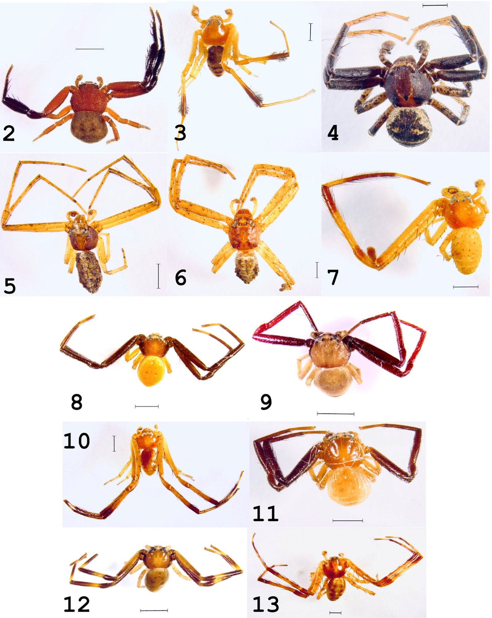
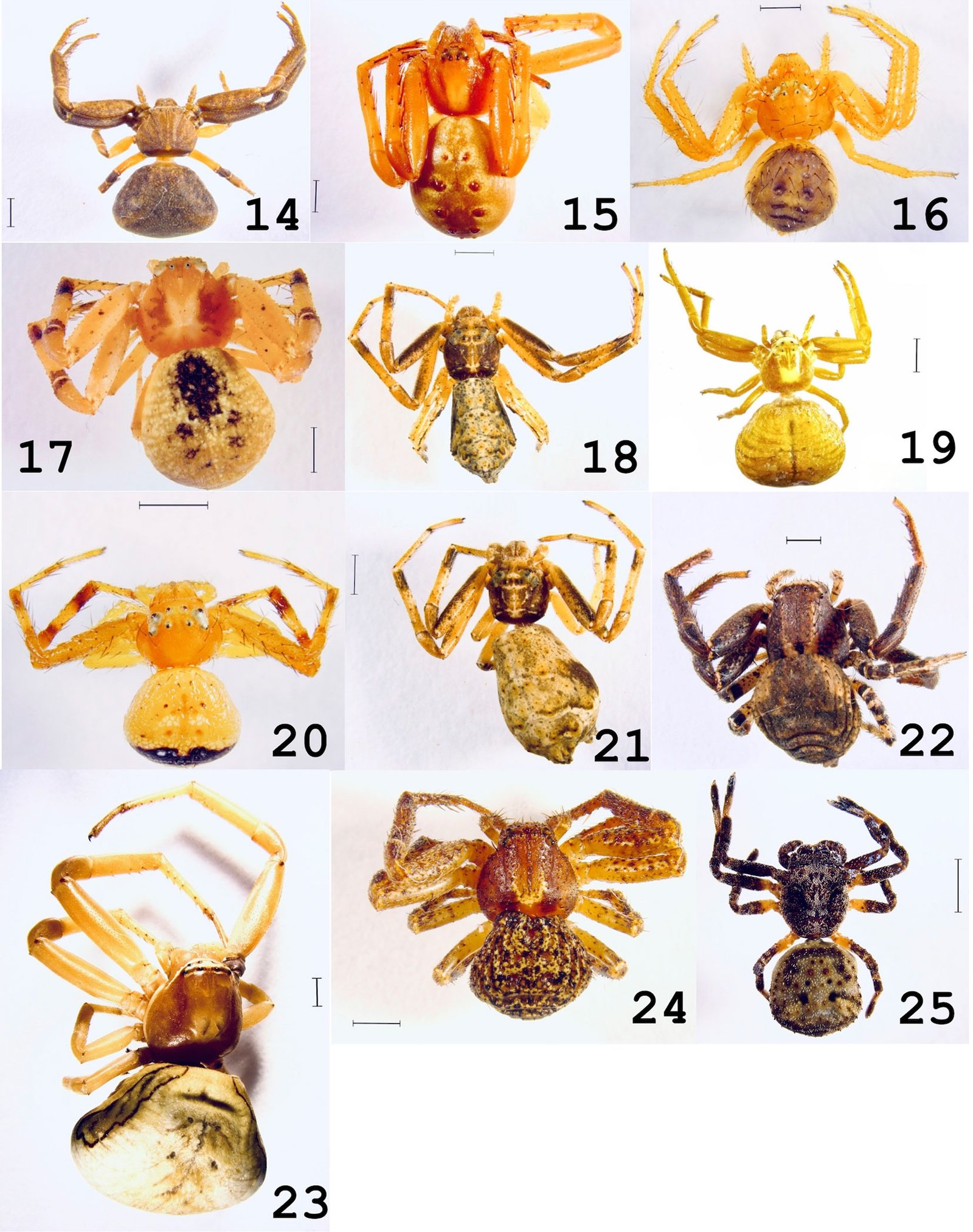
Regarding true diversity, the order-one diversity (¹D) showed that the community was dominated by a few abundant species, with a peak diversity of 5.91 effective species in May, and 3.26 effective dominant species (²D) with a peak diversity of 5.12 effective dominant species in May (Table 2).
The species accumulation curve showed continuous growth without reaching an asymptote, indicating that the true number of species in the study area is greater than what we recorded (Fig. 28). According to the richness estimators (Chao 1, Chao 2, first-order Jackknife, and second-order Jackknife), a richness of 18-20 species is estimated. This suggests that we obtained between 78-88% of the total richness for the Thomisidae family in the studied locality, while 12-22% of the species were not detected.
| Jan | Feb | Mar | Apr | May | Jun | Jul | Aug | Sep | Oct | Nov | Dec | Annual | Dry season | Rainy season | |
|---|---|---|---|---|---|---|---|---|---|---|---|---|---|---|---|
| S | 1 | 2 | – | 7 | 7 | 7 | 10 | 6 | 10 | 7 | 5 | 3 | 16 | 9 | 14 |
| A | 1 | 2 | – | 4 | 13 | 22 | 35 | 20 | 24 | 86 | 18 | 9 | 234 | 47 | 187 |
| ⁰D | 1 | 2 | – | 7 | 7 | 7 | 10 | 6 | 10 | 7 | 5 | 3 | 16 | 9 | 14 |
| ¹D | 1 | 2 | – | 2.83 | 5.91 | 5.93 | 6.66 | 3.56 | 5.99 | 2.12 | 2.85 | 1.98 | 6.56 | 5.08 | 6.29 |
| ²D | 1 | 2 | – | 2.66 | 5.12 | 5.37 | 4.84 | 2.5 | 3.89 | 1.45 | 2.07 | 1.58 | 3.66 | 3.26 | 3.66 |
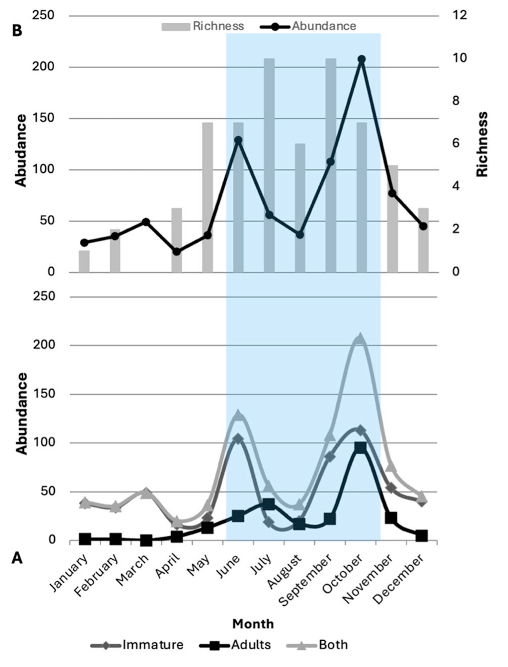
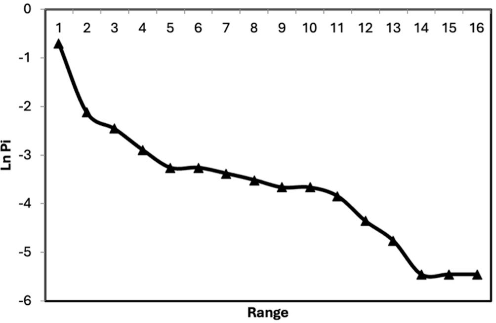
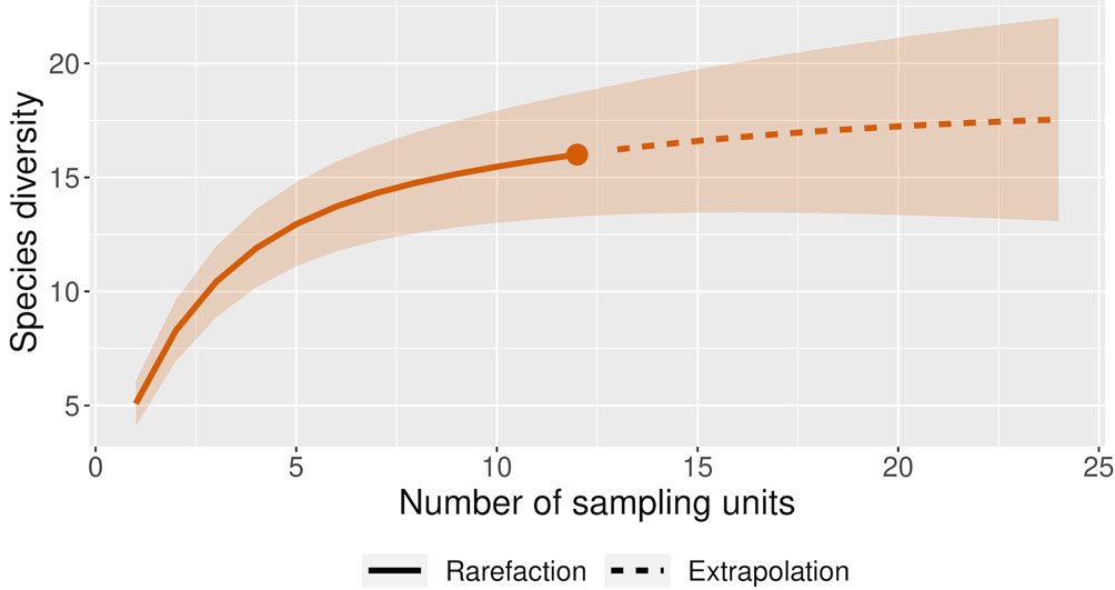
Discussion
Due to the scarce taxonomic information on the spider family Thomisidae in Mexico, the lack of reference collections and specialists, it is not uncommon for faunistic inventories or ecological studies to report a high percentage of unknown or undescribed crab spider species, often with more than 80% of records identified only as morphospecies (Álvarez-Padilla et al., 2020; Argañaraz & Gleiser, 2017; Desales-Lara, 2014; Nieto-Castañeda et al., 2014; Rivera-Quiroz et al., 2016; Rodríguez-Rodríguez et al., 2015). This project reported only 31% of crab spiders as morphospecies. The records presented herein constitute 19% and 61% of the Thomisidae species and genera reported for the country, respectively. Currently, the spider family Thomisidae in Mexico comprises 18 genera and 83 species (World Spider Catalog, 2025); however, more than one-third of Mexican states have no records, or only a few (Pilo-García, 2022). With these results, Morelos now has the fifth highest number of thomisid species in Mexico (16 species), after Veracruz (19), Baja California (19), Chihuahua (19), and Chiapas (16). Previous studies in Mexican deciduous tropical forests recorded the genera Mecaphesa and Synema Simon, 1864 as the most diverse, but herein we found Misumenoides to have the highest species richness, followed by Mecaphesa and Tmarus. We found that Thomisidae individuals are present year-round and are predominantly immature, a common pattern in Araneae. An interesting observation is that the abundance of males was statistically higher than that of adult females; this is uncommon among spiders but has been recorded in the family, and is consistent with the Gravity Hypothesis of extreme sexual size dimorphism in sit-and-wait predators, where smaller males disperse more actively (Corcobado et al., 2010; Hormiga et al., 2000). The marked seasonality, with greater abundance in the rainy than the dry season, aligns with previous thomisid studies (Cardoso et al., 2007; Hernández-Silva, 2016) and tracks the seasonality of the main prey (butterflies and beetles). Rare species were more abundant in the rainy season, whereas more common species were recorded in the dry season, likely reflecting resource (prey) availability. Most species recorded in spider inventories are rare (singletons or doubletons), making it difficult for the accumulation curve to reach the asymptote; evenness factors confirmed the community is predominantly composed of rare species (Jost, 2010), with a singleton proportion of 19%. In conclusion, the family Thomisidae in Morelos is more diverse than previously considered, highlighting the importance of reliable regional faunistic inventories. Using at least 3 techniques with monthly sampling is sufficient to obtain a reliable inventory, even in deciduous tropical forests, although we recommend additional techniques and combining sampling across both seasons to approach the asymptote and obtain comparable data. We consider Thomisidae to be good ecological models given their close association with vegetative strata and their predatory traits; further studies from other localities will broaden understanding of their community structure and its spatial and temporal variation.
Acknowledgements
We thank the following people who helped with fieldwork: García-Márquez V. D., Guzmán-Martínez U. A., Menéndez-Acuña M., Valle-Parra T. A., Uriostegui-Nava E., García-García T. D., Silvestre R., Rodríguez-Herrera B., and Valenzuela C. We also thank A. Hk. Gómez-Calderón for creating the map. We are grateful to Ma. Ventura Echeverría, Ricardo Paredes León, Alejandro Flores Palacios, and Angélica María Corona López for their comments and suggestions. This work would not have been possible without the permission of the community of San Andrés de la Cal. The Facultad de Ciencias Biológicas (UAEM) and the Colección de Insectos de la Universidad de Morelos (CIUM, CIByC) supported this project.
References
Abraham, B. J. (1983). Spatial and temporal patterns in a sagebrush steppe spider community (Arachnida, Araneae). The Journal of Arachnology, 11, 31‒50.
Álvarez-Padilla, F., Galán-Sánchez, M. A., & Salgueiro-Sepúlveda, J. (2020). A protocol for online documentation of spider biodiversity inventories applied to a Mexican tropical wet forest (Araneae: Araneomorphae). Zootaxa, 4722, 241‒269. https://doi.org/10.11646/zootaxa.4722.3.2
Arango, A. M., Rico-Gray, V., & Parra-Tabla, V. (2000). Population structure, seasonality, and habitat use by the green lynx spider Peucetia viridans (Oxyopidae) inhabiting Cnidoscolus aconitifolius (Euphorbiaceae). The Journal of Arachnology, 28, 185‒194.
Argañaraz, C. I., & Gleiser, R. M. (2017). Does urbanization have positive or negative effects on crab spider (Araneae: Thomisidae) diversity? Zoologia, 34, 1‒8. https://doi.org/10.3897/zoologia.34.e19987
Ávalos, G., Rubios, G. D., Bar. M. E., & González, A. (2007). Arañas (Arachnida: Araneae) asociadas a dos bosques degradados del Chaco húmedo en Corrientes, Argentina. Revista de Biología Tropical, 55, 899‒999. https://doi.org/10.15517/rbt.v55i3-4.5965
Balvanera, P., & Maass, M. (2010). Los servicios ecosistémicos que proveen las selvas secas. In G. Ceballos et al. (Eds.), Diversidad, amenazas y áreas prioritarias para la conservación de las selvas secas del Pacífico de México (pp. 251‒271). México, D.F.: Fondo de Cultura Económica.
Benjamin, S. P. (2011). Phylogenetics and comparative morphology of crab spiders (Araneae: Dionycha, Thomisidae). Zootaxa, 3080, 1‒108. https://doi.org/10.11646/zootaxa.3080.1.1
Benjamin, S. P., Dimitrov, D., Gillispie, R. G., & Hormiga, G. (2008). Family ties: molecular phylogeny of crab spiders (Araneae: Thomisidae). Cladistics, 24, 708‒722. https://doi.org/10.1111/j.1096-0031.2008.00202.x
Campuzano, E. F., & Padilla-Ramírez, J. R. (2020). Spatial and seasonal patterns of ground-dwelling spider assemblages belonging to the retrolateral tibial apophysis clade (Araneae: Araneomorphae) in two remnants of pine-oak forest from Mexico. Studies on Neotropical Fauna and Environment, 56, 220‒233. https://doi.org/10.1080/01650521.2020.1806008
Cardoso, P., Henriques, S. S., Gaspar, C., Crespo, L. C., Carvalho, R., Schmidt, J. B. et al. (2007). Species richness and composition assessment of spiders in a Mediterranean scrubland. Journal of Insect Conservation, 13, 45‒55. https://doi.org/10.1007/s10841-007-9116-3
Chao, A., Gotelli, N. J., Hsieh, T. C., Sander, E. L., Ma, K. H., Colwell, R. K. et al. (2014). Rarefaction and extrapolation with Hill numbers: a framework for sampling and estimation in species diversity studies. Ecological Monographs, 84, 45–67. https://doi.org/10.1890/13-0133.1
Chao, A., Ma, K. H., & Hsieh, T. C. (2016). iNEXT Online: software for interpolation and extrapolation of species diversity. http://chao.stat.nthu.edu.tw/wordpress/software_download/inext-online/
Clausen, I. H. S. (1986). The use of spiders (Araneae) as ecological indicators. Bulletin of the British Arachnological Society, 7, 83‒86.
Coddington, J. A., Agnarsson, I., Miller, J. A., Kuntner, M., & Hormiga, G. (2009). Undersampling bias: the null hypothesis for singleton species in tropical arthropod surveys. Journal of Animal Ecology, 78, 573‒584. https://doi.org/10.1111/j.1365-2656.2009.01525.x
Coddington, J. A., Young, L. H., & Coley, F. A. (1996). Estimating spider species richness in a southern Appalachian cove hardwood forest. The Journal of Arachnology, 24, 111‒128.
Colwell, R. K. (2013). EstimateS: statistical estimation of species richness and shared species from samples. Version 9. http://purl.oclc.org/estimates
Colwell, R. K., & Coddington, J. A. (1994). Estimating terrestrial biodiversity through extrapolation. Philosophical Transactions of the Royal Society of London B, 345, 101‒118.
Connell, J. H. & Orias, E. (1964). The ecological regulation of species diversity. The American Naturalist, 98, 399‒414. https://doi.org/10.1086/282335
Corcobado, G., Rodríguez-Gironés, M. A., de Mas, E., & Moya-Laraño, J. (2010). Introducing the refined gravity hypothesis of extreme sexual size dimorphism. BMC Evolutionary Biology, 10, 236. https://doi.org/10.1186/1471-2148-10-236
Corcuera, P., Jiménez, M. L., & Desales-Lara, M. A. (2019). The spiders of the Churince Region, Cuatro Ciénegas Basin. In F. Alvarez, & M. Ojeda (Eds.), Animal diversity and biogeography of Cuatro Ciénegas Basin (pp. 61‒75). Springer Nature. https://doi.org/10.1007/978-3-030-11262-2_5
Corona-López, A. M., Reza-Pérez, E. V., Toledo-Hernández, V. H., Flores-Palacios, A., Macrae, T. C., Westcott, R. L. et al. (2017). Diversity of Buprestidae (Coleoptera) from El Limón de Cuauchichinola, Tepalcingo, Morelos, Mexico. The Pan-Pacific Entomologist, 93, 71‒83. https://doi.org/10.3956/2017-93.2.71
Cortez-Hernández, A. G. (2019). Diversidad y distribución de la familia Thomisidae (Arachnida: Araneae) de la sierra de Zongolica, Veracruz (Bachelor’s Thesis). FES Zaragoza, UNAM, CDMX.
Desales-Lara, M. A. (2014). Araneofauna (Arachnida: Araneae) del Estado de México, México. Acta Zoológica Mexicana, 30, 298‒320. https://doi.org/10.21829/azm.2014.302104
Desales-Lara, M. A., Francke, O. F., & Sánchez-Nava, P. (2013). Diversidad de arañas (Arachnida: Araneae) en hábitats antropogénicos. Revista Mexicana de Biodiversidad, 84, 291‒305. https://doi.org/10.7550/rmb.31708
Durán-Barrón, C. G., Francke, O. F., & Pérez-Ortiz, T. M. (2009). Diversidad de arañas (Arachnida: Araneae) asociadas con viviendas de la Ciudad de México (Zona Metropolitana). https://doi.org/10.22201/ib.20078706e.2009.001.584
Esquivel-Gómez, L., Abdala-Robles, L., Pinkus-Rendón, M., & Parra-Tabla, V. (2016). Effects of tree species diversity on a community of weaver spiders in a tropical forest plantation. Biotropica, 1‒18. https://doi.org/10.1111/btp.12352
Francke, O. F. (2014). Biodiversidad de Arthropoda (Chelicerata: Arachnida ex Acari) en México. Revista Mexicana de Biodiversidad, 85 (Suppl.), 408‒418. https://doi.org/10.7550/rmb.31914
García-García, M. A., Ibarra-Núñez, G., Martínez-Matínez, L., Santos-Moreno, A., & Sánchez-García, J. A. (2023). Spider diversity (Arachnida: Araneae) in two different coffee management systems and surrounding tropical forest during two contrasting seasons in Oaxaca, Mexico. Acta Zoológica Mexicana, 39, 1‒25. https://doi.org/10.21829/azm.2023.3912584
García, E. (2004). Modificaciones al sistema de clasificación climática de Köppen. Instituto de Geografía. Ciudad de México: UNAM.
Gertsch, W. J. (1953). The spider genera Xysticus, Choriarachne and Oxyptila (Thomisidae: Misumeninae) in North America. The American Museum of Natural History, 102, 413‒482.
Gertsch, W. J., & Davis, L. I. (1940). Report on a collection of spiders from Mexico III. The American Museum of Natural History, 1069, 1‒22.
González-Castillo, M. P., Pérez-Santiago, G., & Correa-Ramírez, M. M. (2014). Inventario preliminar sobre el orden Araneae (Arachnida) en comunidades semiáridas de los valles de Durango, Dgo. México. Entomología Mexicana, 1, 26‒31.
Gotelli, N. J., & Cowell, R. K. (2011). Estimating species richness. In A. E. Magurran, & B. J. McGill (Eds.), Biological diversity: frontiers in measurement and assessment (pp. 34‒335). New York: Oxford Press.
Halaj, J., Ross, D. W., & Moldenke A. R. (1998). Habitat structure and prey availability as predictors of the abundance and community organization of spiders in Western Oregon forest canopies. Journal of Arachnology, 26, 203‒220.
Hernández-Silva, Y. G. (2016). Araneofauna de vegetación en tratamientos de restauración ecológica en selva estacional de Sierra de Huautla, Morelos (Bachelor’s Thesis). Facultad de Ciencias Biológicas, UAEM, Cuernavaca.
Hoffmann, A. (1976). Relación bibliográfica preliminar de las arañas de México (Arachnida, Araneae). Publicaciones Especiales Núm. 3. México D.F.: Instituto de Biología, UNAM.
Hormiga, G., Scharff, N., & Coddington, J. A. (2000). The phylogenetic basis of sexual size dimorphism in orb-weaving spiders (Araneae, Orbiculariae). Systematic Biology, 49, 435‒462.
Jiménez, M. L. (1986). Descripción de una nueva especie de la familia Thomisidae (Arachnida: Araneae) de México. Anales del Instituto de Biología, UNAM, Serie Zoología, 56, 11‒14.
Jiménez, M. L. (1992). New species of crab spider from Baja California Sur (Araneae: Thomisidae). The Journal of Arachnology, 20, 50‒57.
Jiménez, M. L. (1996). Araneae. In J. Llorente-Bousquets et al. (Eds.), Biodiversidad, taxonomía y biogeografía de artrópodos de México (pp. 83‒101). México, D.F.: Conabio.
Jiménez, M. L., Chamé-Vázquez, D., Palacios-Cardiel, C., & Van-Devender, T. R. (2024). Spiders (Arachnida: Araneae) from the Sky Island Mountains of Sonora. The Pan-Pacific Entomologist, 100, 175‒211. https://doi.org/10.3956/2024-100.3.175
Jiménez, M. L., Palacios-Cardiel, C., & Chávez-Lara, I. D. (2020). Las arañas (Arachnida: Araneae) de los Médanos de Samalayuca, Chihuahua y nuevos registros de especies para México. Acta Zoológica Mexicana, 36, 1‒23. https://doi.org/10.21829/azm.2020.3612205
Jiménez-Valverde, A., & Hortal, J. (2003). Las curvas de acumulación de especies y la necesidad de evaluar la calidad de los inventarios biológicos. Revista Ibérica de Aracnología, 8, 151‒161.
Jiménez-Valverde, A., & Lobo, J. M. (2004). Un método sencillo para seleccionar puntos de muestreo con el objetivo de inventariar taxones hiperdiversos: el caso práctico de las familias Araneidae y Thomisidae (Araneae) en la comunidad de Madrid, España. Ecología, 18, 297‒308.
Jiménez-Valverde, A., & Lobo, J. M. (2005). Determining a combined sampling procedure for a reliable estimation of Araneidae and Thomisidae assemblages (Arachnida: Araneae). The Journal of Arachnology, 33, 33‒42. https://doi.org/10.1636/M03-10
Jiménez-Valverde, A., & Lobo, J. M. (2007). Determinants of local spider (Araneidae and Thomisidae) species richness on a regional scale: climate and altitude vs. habitat structure. Ecological Entomology, 32, 113‒122. https://doi.org/10.1111/j.1365-2311.2006.00848.x
Jocqué, R., & Dippenaar-Schoeman, A. S. (2006). Spider families of the world. Belgium: Royal Museum of Central Africa.
Jost, L. (2006). Entropy and diversity. Oikos, 113, 363‒375. https://doi.org/10.1111/j.2006.0030-1299.14714.x
Jost, L. (2010). The relation between evenness and diversity. Diversity, 2, 207‒232. https://doi.org/10.3390/d2020207
Jost, L., & González-Oreja, J. A. (2012). Midiendo la diversidad biológica: más allá del índice de Shannon. Acta Zoológica Lilloana, 56, 3‒14.
Lapp, T. J., & Dondale, C. D. (2017). Thomisidae. In D. Ubick, P. Paquin, P. E. Cushing, & V. Roth (Eds.), Spiders of North America: an identification manual (pp. 272‒273). Keene, New Hampshire: American Arachnological Society.
Llinas-Gutiérrez, J., & Jiménez, M. L. (2004). Arañas de humedales del sur de Baja California, México. Anales del Instituto de Biología, UNAM, Serie Zoología, 75, 283‒302.
Lopes-Rodrigues, E. N., Marques-Pires, M., & de Souza-Mendonça, M. J. (2023). Seasonal changes in spider diversity in subtropical riparian forest. The Journal of Arachnology, 51, 19‒26. https://doi.org/10.1636/JoA-S-21-049
Luna-Reyes, M., Llorente-Bousquets, J., & Luis-Martínez, A. (2008). Papilionidae de la Sierra de Huautla, Morelos y Puebla, México (Insecta: Lepidoptera). Revista de Biología Tropical, 56, 1677‒1716.
Maldonado-Carrizales, J., Ponce-Saavedra, J., & Valdez-Mondragón, A. (2021). Riqueza y abundancia de arañas (Arachnida: Araneae) en ambientes urbanos y su vegetación aledaña al poniente de la ciudad de Morelia, Michoacán, México. Revista Mexicana de Biodiversidad, 92, 1‒18. https://doi.org/10.22201/ib.20078706e.2021.92.3650
Martínez-Hernández, J. G., Corona-López, A. M., Flores-Palacios, A., Rös, M., & Toledo-Hernández, V. H. (2019). Seasonal diversity of Cerambycidae (Coleoptera) is more complex than thought. PeerJ, 7, e7866. https://doi.org/10.7717/peerj.7866
Martínez-Hernández, J. G., Corona-López, A. M., Flores-Palacios, A., & Toledo-Hernández, V. H. (2022). Structure of Cerambycidae (Coleoptera) community in a tropical deciduous forest in northern Morelos, Mexico. Annals of the Entomological Society of America, 20, 1‒8. https://doi.org/10.1093/aesa/saac005
Maya-Morales, J., Ibarra-Núñez, G., León-Cortés, J. L., & Infante, F. (2012). Understory spider diversity in two remnants of tropical montane cloud forest in Chiapas, Mexico. Journal of Insect Conservation, 16, 25‒38. https://doi.org/10.1007/s10841-011-9391-x
Menéndez-Acuña, M. (2017). Efecto de la diversidad genética de una especie fundadora sobre la comunidad de plantas y arañas asociadas (M.Sc. Thesis). CIByC, UAEM, México.
Menéndez-Acuña, M., Salas-Rodríguez, M., Montiel-Parra, G., Sotuyo, S., & Rosas-Echeverría, M. V. (2023). Seasonality and long-term effect of environmental variables on the orb weaver spider community of a tropical dry forest in the Balsas Basin, Mexico. Diversity, 15, 466. https://doi.org/10.3390/d15030466
Miranda, F., & Hernández, X. E. (1963). Los tipos de vegetación en México y su clasificación. Boletín de la Sociedad Botánica de México, 28, 29‒179. https://doi.org/10.17129/botsci.1084
Morse, D. H. (2007). Predator upon a flower: life history and fitness in a crab spider. Cambridge, MA: Harvard University Press.
Nadal, M. F., Achitte-Schmutzler, H. C., Zanone, I., González, P. I., & Ávalos, G. (2018). Diversidad estacional de arañas en una reserva natural del Espinal en Corrientes, Argentina. Caldasia, 40, 129‒143.
Nieto-Castañeda, I. G., Pérez-Miguel, L., & García-Cano, A. A. (2014). New records of spiders (Arachnida: Araneae) from the Balsas Basin in central Mexico. The Southwestern Naturalist, 59, 426‒430. https://doi.org/10.1894/JC-77.1
Orozco-Gil, M., & Desales-Lara, M. A. (2021). Las arañas (Arachnida: Araneae) del estado de Hidalgo, México. Acta Zoológica Mexicana (N.S.), 31, 1‒23. https://doi.org/10.21829/azm.2023.3912583
Pérez-Hernández, C. X., & Zaragoza-Caballero, S. (2016). Temporal variation in the diversity of Cantharidae (Coleoptera) in seven assemblages in tropical dry forest in Mexico. Tropical Conservation Science, 9, 439‒464. https://doi.org/10.1177/194008291600900124
Pickard-Cambridge, F. O. (1895-1903). Arachnida: Araneidea and Opiliones. Biologia Centrali Americana, 2, 89‒214.
Pickard-Cambridge, O. (1896). Arachnida-Araneidea. Biologia Centrali Americana, 1, 57‒288.
Pilo-García, F. (2022). Estructura de la comunidad de la familia Thomisidae (Arachnida: Araneae) en San Andrés de la Cal, Tepoztlán, Morelos (Bachelor’s Thesis). Facultad de Ciencias Biológicas, UAEM, Cuernavaca.
Piña-Rodríguez, O. P., García-Cano, A. A., & Espinosa-Organista, D. H. (2015). Inventario de arañas (Arachnida: Araneae) de la zona noroeste de Guerrero, México. Boletín de la Sociedad Mexicana de Entomología, 1, 26‒32.
Ponce-Saavedra, J. et al. (2023). The fauna of Arachnids in the Anthropocene of Mexico. In R. W. Jones et al. (Eds.), Mexican Fauna in the Anthropocene (pp. 17–46). Cham: Springer. https://doi.org/10.1007/978-3-031-17277-9_2
R Core-Team (2024). R: a language and environment for statistical computing. R Foundation for Statistical Computing, Vienna, Austria. https://www.r-project.org/
Reyes-González, R., Toledo-Hernández, V. H., Flores-Palacios, A., Rös, M., Bueno-Villegas, J., & Corona-López, A. M. (2024). Exploring the proportion of rarity in tropical insects. Écoscience, 1‒10. https://doi.org/10.1080/11956860.2024.2435133
Rivas-Herrera, C. I. (2015). Araneofauna errante (Arachnida: Araneae) en tratamientos de restauración ecológica en la selva estacional de Sierra de Huautla, México (Bachelor’s Thesis). Facultad de Ciencias Biológicas, UAEM, Cuernavaca.
Rivera-Quiroz, F. A., Garcilazo-Cruz, U., & Álvarez-Padilla, F. (2016). Spider cyberdiversity (Araneae: Araneomorphae) in an ecotouristic tropical forest fragment in Xilitla, Mexico. https://doi.org/10.1016/j.rmb.2016.07.011
Rodríguez-Rodríguez, S. E., Solís-Catalán, K. P., & Valdez-Mondragón, A. (2015). Diversity and seasonal abundance of anthropogenic spiders (Arachnida: Araneae) in different urban zones of the city of Chilpancingo, Guerrero, México. https://doi.org/10.1016/j.rmb.2015.09.002
Rosas-Echeverría, M. V., Coyote-Ávila, C. A., Aguilar-Dorantes, K. M., & Martínez-Peralta, C. (2019). Diversity of butterflies (Lepidoptera) in Sierra de Huautla, Morelos, México. Annals of the Entomological Society of America, 112, 409‒417. https://doi.org/10.1093/aesa/saz022
Ruiz-Rivera, C. A. (2001). San Andrés de la Cal: culto a los señores del tiempo en rituales agrarios. Cuernavaca, Morelos: UAEM.
Samu, F., & Lövei, G. L. (1995). Species richness of a spider community (Araneae). European Journal of Entomology, 92, 633‒638.
Silva, D., & Coddington, J. A. (1996). Spiders of Pakitza (Madre de Dios, Perú). In D. E. Wilson, & A. Sandoval (Eds.), The biodiversity of southeastern Perú (pp. 253‒308). Washington, D.C.: Smithsonian Institute.
Sørensen, L. L. (2002). Stratification of the spider fauna in a Tanzanian forest. In Y. Basset et al. (Eds.), Arthropods of tropical forest (pp. 92‒101). Cambridge, UK: Cambridge University Press.
Trejo, I. (2010). Las selvas secas del Pacífico mexicano. In G. Ceballos et al. (Eds.), Diversidad, amenazas y áreas prioritarias para la conservación de las selvas secas del Pacífico de México (pp. 41‒51). México, D.F.: Fondo de Cultura Económica.
Turnbull, A. L. (1973). Ecology of the true spiders (Araneomorphae). Annual Review of Entomology, 18, 305‒348. https://doi.org/10.1146/annurev.en.18.010173.001513
Ubick, D., Paquin, P., Cushing, P. E., & Roth, V. (2017). Spiders of North America: an identification manual, 2nd Edition. New Hampshire: American Arachnological Society.
Vergara-Torres, C. A., Pacheco-Álvarez, M. C., & Flores-Palacios, A. (2010). Host preference and host limitation of vascular epiphytes in a tropical dry forest of central Mexico. Journal of Tropical Ecology, 26, 563‒570. https://doi.org/10.1017/S0266467410000349
Williams, P. H., & Gaston, K. J. (1994). Measuring more of biodiversity: can higher-taxon richness predict wholesale species richness? Biological Conservation, 67, 211‒217. https://doi.org/10.1016/0006-3207(94)90612-2
Wolda, H. (1988). Insect seasonality: why? Annual Review of Ecology and Systematics, 19, 1‒18. https://doi.org/10.1146/annurev.es.19.110188.000245

Identificación molecular de lombrices de tierra composteras usando código de barras de DNA
Molecular identification of composting earthworms using DNA barcoding
Mayela Martínez-Cano a, *, Ana Elena Dorantes-Acosta a, Sergio Martínez-Hernández a, José Antonio García-Pérez b, Huemantzin Balan Ortiz-Oliveros c y Angel Isauro Ortiz-Ceballos a
a Universidad Veracruzana, Instituto de Biotecnología y Ecología Aplicada, Av. de las Culturas Veracruzanas 101, Col. Emiliano Zapata, 91090 Xalapa, Veracruz, México
b Universidad Veracruzana, Facultad de Biología, Circuito Universitario Gonzalo Aguirre Beltrán, Zona Universitaria, 91090 Xalapa, Veracruz, México
c Instituto Nacional de Investigaciones Nucleares, Departamento de Química, La Marquesa, 52750 Ocoyoacac, Estado de México, México
*Autor de correspondencia: maymartinez@uv.mx (M. Martínez-Cano)
Recibido: 30 agosto 2025; aceptado: 4 marzo 2026
Resumen
Las lombrices de tierra composteras desempeñan un papel clave en la descomposición de la materia orgánica, las especies epigeas del género Eisenia son utilizadas ampliamente para efectuar el proceso de lombricompostaje y como bioindicadores en los estudios toxicológicos. Sin embargo, la identidad taxonómica precisa de las especies (semejanza morfológica) representa un desafío y puede afectar la eficacia y función del proceso de lombricompostaje. En este estudio se determinó la identidad de lombrices presentes en 5 instalaciones de vermicompostaje de Veracruz y Quintana Roo, México, empleando análisis molecular basado en la secuenciación del gen mitocondrial COI. El análisis reveló la presencia de 2 especies, Eisenia andrei y Perionyx excavatus, descartando la presencia de Eisenia fetida, la especie asumida previamente por encargados de las plantas de lombricompostaje. Las distancias génicas fueron < 1.3%, mientras que las divergencias con E. fetida superaron 16%, lo que valida la delimitación específica. Nuestros resultados destacan la necesidad de integrar métodos moleculares en la identificación de lombrices de tierra para su uso en los estudios toxicológicos y fortalecer el manejo sostenible de residuos orgánicos.
Palabras clave: Residuos orgánicos; Taxonomía; Especies epigeas
Abstract
Composting earthworms play a key role in the decomposition of organic matter. Epigeic species of the genus Eisenia are widely used both in vermicomposting and as bioindicators in toxicological studies. However, accurate taxonomic identification of these species remains challenging due to their high morphological similarity, which affects the efficiency and function of vermicomposting processes. In this study, the earthworm species present in 5 vermicomposting facilities located in Veracruz and Quintana Roo, México, were identified through molecular analyses of the mitochondrial COI gene. The results revealed the presence of 2 species: Eisenia andrei and Perionyx excavatus, ruling out Eisenia fetida, which had previously been assumed by facility operators. Genetic distances between the identified specimens were below 1.3%, while divergences from E. fetida exceeded 16%, supporting clear species delimitation. Our results highlight the need to integrate molecular methods into earthworm identification for their use in toxicological studies and to strengthen the sustainable management of organic waste.
Keywords: Organic waste; Taxonomy; Epigean species
Introducción
Las lombrices de tierra desempeñan un papel fundamental en los ecosistemas terrestres debido a su contribución a la descomposición de la materia orgánica y a la mejora de las propiedades fisicoquímicas del suelo (Fragoso y Rojas, 2014). Por su relevancia ecológica ha motivado un interés creciente por comprender su diversidad y distribución global. Hasta la fecha, se han descrito alrededor de 5,700 especies de lombrices de tierra, aunque se considera que la diversidad real podría ser mucho mayor debido a la falta de taxonomía y la presencia de especies crípticas (Misirlioğlu et al., 2023). Esta diversidad refleja la adaptación de las lombrices de tierra a distintos hábitats y su uso potencial en diversas aplicaciones biotecnológicas. Las lombrices de tierra epigeas habitan principalmente la hojarasca y se alimentan de materia orgánica en descomposición. Debido a estas características, varias especies han sido empleadas en prácticas sostenibles para el manejo de residuos orgánicos, particularmente en procesos de lombricompostaje (Domínguez y Edwards, 2004). La lombricomposta es el producto de la transformación biológica de residuos orgánicos en biofertilizantes ricos en nutrientes, proceso en el cual las lombrices desempeñan un papel central. No obstante, las especies epigeas utilizadas en lombricompostaje presentan diferencias importantes en su comportamiento, tolerancia ambiental y eficiencia en la degradación de los residuos, lo que genera variabilidad interespecífica en el rendimiento del proceso (Suthar y Singh, 2008). En la región de alta montaña del centro de Veracruz, el lombricompostaje de residuos orgánicos se desarrolló inicialmente a partir del aprovechamiento de la pulpa de café. Durante esta etapa, las lombrices empleadas fueron identificadas morfológicamente como Eisenia fetida (Savigny, 1826) y Metaphire californica (Aranda, 1988). Sin embargo, revisiones taxonómicas posteriores corrigieron dichas identificaciones, demostrando que las poblaciones utilizadas correspondían en realidad a Eisenia andrei (Aranda et al., 1999, 2011). Estos antecedentes evidencian las limitaciones de la identificación basada exclusivamente en criterios morfológicos. De manera paralela, en una instalación de lombricompostaje ubicada en Playa del Carmen, Quintana Roo, se emplean lombrices de tierra para el tratamiento de residuos orgánicos de origen vegetal y animal. En estos sistemas, la identificación de las especies también se ha basado principalmente en la apreciación empírica de los operadores, quienes las reconocen de forma tentativa como E. fetida y asumen que su eficacia en el proceso constituye evidencia suficiente de su identidad taxonómica. Sin embargo, esta práctica puede ser errónea, especialmente cuando se trata de especies morfológicamente similares. Diversas especies de lombrices de tierra han demostrado potencial para la producción de lombricomposta (Domínguez y Edwards, 2004), entre ellas destacan Lumbricus rubellus (Hoffmeister, 1843), Dendrobaena rubida (Savigny, 1826), Eudrilus eugeniae (Kinberg, 1867), Eiseniella tetraedra (Savigny, 1826), Perionyx excavatus (Perrier, 1872), E. fetida y E. andrei (Bouché, 1972). No obstante, no todas las especies aptas para lombricompostaje son esperables en la región; en Veracruz se han registrado principalmente poblaciones de E. fetida y E. andrei en acumulaciones de pulpa de café (Fragoso, 2011). Mientras que especies tropicales como P. excavatus o E. euginae son más habituales en climas cálidos de baja altitud (por ejemplo, Quintana Roo). Especies de origen templado, por ejemplo L. rubellus, D. rubida, E. tetraedra son menos probables en la región, salvo en casos de introducción o microhábitats específicos (Fragoso y Rojas, 2014). Además, la coexistencia de múltiples especies con morfologías similares sugiere que la identificación basada únicamente en criterios visuales puede ser inexacta, lo que resalta la necesidad de emplear herramientas de diagnóstico más precisas. La identificación taxonómica de lombrices de tierra continúa siendo un desafío, especialmente entre especies estrechamente relacionadas. Un caso particularmente relevante es el de E. fetida y E. andrei, 2 especies ampliamente utilizadas en lombricompostaje, ecotoxicología, fisiología y genética. Varias investigaciones han demostrado de manera concluyente que se trata de especies biológicas distintas, aisladas reproductivamente (Domínguez et al., 2005). Asimismo, los análisis filogenéticos basados en los genes 28S y COI (citocromo c oxidasa subunidad I) han corroborado su diferenciación evolutiva (Domínguez y Pérez-Losada, 2010). El reconocimiento de E. fetida y E. andrei como especies distintas tiene implicaciones relevantes. En procesos de lombricompostaje, se ha documentado que E. andrei presenta tasas de crecimiento y reproducción superiores a las de E. fetida (García et al., 2019), lo que la convierte en una opción más eficiente para el tratamiento de residuos orgánicos. Asimismo, en estudios de ecotoxicología no es posible asumir respuestas equivalentes frente a contaminantes, ya que diferentes especies de lombrices pueden diferir en su sensibilidad y fisiología (Zhang et al., 2022). El método tradicional para clasificar las especies se basa en rasgos morfológicos como la pigmentación y las estructuras reproductivas; sin embargo, son características que pueden ser ambiguas y estar afectadas por el ambiente, lo que puede llevar a cometer errores para su identificación (Domínguez et al., 2005). Con base en estas limitaciones de la taxonomía morfológica, se emplean cada vez más técnicas moleculares para distinguir y diferenciar entre especies morfológicamente semejantes. El gen mitocondrial de la subunidad I de la citocromo c oxidasa (COI) se ha utilizado ampliamente como marcador molecular para la identificación de especies debido a su alta divergencia interespecífica y baja variación intraespecífica (James et al., 2010). Los análisis filogenéticos basados en secuencias del gen COI han demostrado ser eficaces para resolver incertidumbres taxonómicas dentro del género Eisenia, ofreciendo un enfoque confiable para la identificación de especies y estudios evolutivos (King et al., 2008). Así, la técnica molecular aporta información relevante para conocer con seguridad la diversidad de lombrices de tierra en sistemas de lombricompostaje y se respalda su uso en prácticas sostenibles de manejo de residuos orgánicos. Dada la importancia de una identificación taxonómica precisa para estudios ecológicos, ecotoxicológicos y aplicaciones biotecnológicas, el presente estudio tuvo como objetivo determinar, mediante un enfoque molecular, la identidad de las lombrices de tierra utilizadas en 4 plantas de vermicompostaje en el centro de Veracruz y una en Quintana Roo, México.
Materiales y métodos
Las lombrices de tierra composteras fueron recolectadas en diversas plantas de lombricompostaje, donde los propietarios y/o responsables las identifican de manera general como E. fetida. Las instalaciones seleccionadas para el estudio incluyen la Unidad de Capacitación para el Desarrollo Rural (MMCA), la Planta de Lombricomposta Teocelo (MMTO), la tienda “Hongos de las Altas Montañas” (MMFT), la Lombricomposta Olmos (MMOL) y Rancho Balam (MMBA). La información correspondiente a la ubicación, altitud, condiciones climáticas, rango de temperatura y sustrato principal de cada instalación se presenta en la tabla 1.
En cada una de las plantas de lombricompostaje (MMCA, MMTO, MMFT, MMOL y MMBA) se recolectó aproximadamente 1 kg de sustrato que contenía lombrices de tierra, constituido como muestra compuesta, obtenida al tomar una muestra de cada una de las camas de lombricompostaje presentes en cada planta. Éste fue transportado en cajas de plástico al Instituto de Biotecnología y Ecología Aplicada (INBIOTECA). En el laboratorio, cada muestra se mantuvo de manera aislada en condiciones controladas utilizando pulpa de café como sustrato (Aranda y Barois, 2000).
A los 60 días de cultivo, en cada uno de los 5 cultivos de lombricomposta se recolectaron 3 lombrices de tierra sanas y sexualmente maduras. Las lombrices de tierra fueron lavadas suavemente con agua corriente para eliminar restos de materia orgánica, después se sumergieron en formol 4%. A las 24 h se realizó la descripción taxonómica con el apoyo de un estereomicroscopio para identificar posibles diferencias morfológicas externas (tamaño corporal, número de segmentos, coloración, posición del clitelo y los tubérculos pubertarios) entre los especímenes recolectados en cada cultivo (Moreno y Borges, 2004). Todas las lombrices de tierra fueron preservadas y depositadas en el INBIOTECA.
Se recolectaron 15 lombrices de tierra (3 por cada unidad de lombricompostaje), enjuagadas suavemente con agua corriente, colocadas en tubos de ensayo con etanol 96% y conservadas a -18 °C hasta su uso. Las lombrices de tierra composteadoras fueron identificadas utilizando la técnica de código de barras genético basada en la secuenciación del gen mitocondrial de la subunidad I del citocromo c oxidasa (650-653 pb). Para ello, se utilizó el método estandarizado por Römbke et al. (2016), ISO (2019) y Prosser et al. (2013). Primero, se cortó una sección de 4 mm del tejido de la cola de 5 lombrices de cada lote utilizando un bisturí. La extracción de DNA se realizó empleando el método de extracción HotShot (Montero-Pau et al., 2008). La concentración de DNA se midió con absorbancia a 260 nm usando un espectrofotómetro GeneQuant II (Pharmacia Biotech Co.).
La reacción en cadena de la polimerasa (PCR) se llevó a cabo siguiendo el protocolo descrito por DeWaard et al. (2008). El gen COI se amplificó utilizando los cebadores ZplankF1_t1 y ZplankR1_t1 (Prosser et al., 2013). La mezcla de reacción de PCR tuvo un volumen total de 10.37 µL, que contenía: 2 µL de agua ultrapura, 6.25 µL de trehalosa al 10%, 1.25 µL de tampón 10X, 0.625 µL de MgCl2 (50 mM), 0.0625 µL de dNTPs (10 mM), 0.125 µL de cada cebador (10 µM) y 0.06 µL de la enzima Platinum Taq DNA polimerasa. Se añadieron 3 µL de DNA de cada muestra a la mezcla de PCR, obteniéndose un volumen final de 13.5 µL por tubo (10.5 µL de mezcla de PCR y 3 µL de DNA). Los tubos para PCR se colocaron en un termociclador Eppendorf con el siguiente programa: desnaturalización inicial a 94 °C durante 1 min; 5 ciclos de: 94 °C por 40 s, 45 °C por 40 s, y 72 °C por 1 min; 35 ciclos de: 94 °C por 40 s, 51 °C por 40 s, y 72 °C por 1 min; extensión final a 72 °C durante 5 min.
Los productos de la PCR se visualizaron en un gel de agarosa precargado 2% (E-Gel, Invitrogen). La secuenciación se realizó utilizando el kit BigDye© Terminator v.3.1, seguido de una secuenciación bidireccional en un secuenciador automático ABI 3730XL. Las secuencias obtenidas (650-653 pb) fueron editadas con el software CodonCode v.3.0.1 (CodonCode Corporation, Dedham, MA, EE.UU.) y posteriormente subidas a la base de datos Barcode of Life Database (BOLD, boldsystems.org), donde están disponibles en el conjunto de datos Taxonomic Identification of Annelids (TIAMD). Todas las secuencias que cumplieron con los estándares mínimos de calidad (> 500 pb, < 1% de bases ambiguas, sin codones de paro ni contaminación) fueron asignadas a un número de índice de código de barras (BIN) en BOLD (Ratnasingham y Hebert, 2013).
Con base en Römbke et al. (2016), se incorporaron secuencias de referencia de Eisenia andrei (JN869997.1 y AY874511.1) y Eisenia fetida 1 y 2 (AY874513.1 y AY874515.1), las cuales son ampliamente utilizadas como referencias en laboratorios de pruebas ecotoxicológicas ISO-21286 (ISO, 2019). Para P. excavatus, se utilizó una secuencia de referencia disponible en BOLD (EWSJA764-08); además, se incluyó una secuencia adicional de E. andrei disponible en BOLD Systems (GBAN0383-06). Posteriormente, se realizó el cálculo de las distancias génicas entre las secuencias, se estimaron utilizando el software Mega v7.0 (Kumar et al., 2016) y se evaluó la confiabilidad de las estimaciones de distancia, se realizaron 1,000 réplicas bootstrap. Las matrices de distancia obtenidas se usaron en los análisis comparativos entre grupos. Las secuencias fueron alineadas previamente utilizando ClustalW incorporado en Mega. Finalmente, la identificación molecular se realizó usando un fenograma Neighbor-Joining (NJ) con 1,000 réplicas bootstrap en Mega v7.0 (Kumar et al., 2016).
| Planta de lombricompostaje | Ubicación | Altitud (m snm) | Clima | Temperatura (°C) | Fuente de alimento |
|---|---|---|---|---|---|
| UNCADER | Coatepec, Ver. (19°27’46.7” N, 96°58’2” O) | 1,200-1,270 | Templado-húmedo | 10 – 29 | Residuos de hojarasca |
| Teocelo | Teocelo, Ver. (19°22’43.3” N, 96°57’55.5” O) | 1,107 | Templado-húmedo | 10 – 30 | Residuos de frutas y verduras |
| Tienda Hongos | Fortín de las Flores, Ver. (18°54’50” N, 96°59’27” O) | 1,000-1,070 | Cálido-subhúmedo | 22 – 31 | Residuos del cultivo de setas y estiércol de ganado |
| Olmos | San Marcos de León, Ver. (19°25’25.2” N, 96°57’50.6” O) | 1,145-1,320 | Cálido-subhúmedo | 20 – 32 | Pulpa de café |
| Rancho Balam | Playa del Carmen, Quintana Roo (20°47’00.8” N, 86°57’27.5” O) | Nivel del mar | Cálido-húmedo | 25.5 – 28 | Estiércol de ganado |
Resultados
De las 15 lombrices de tierra estudiadas, los 3 especímenes procedentes de la planta MMFT mostraron diferencias evidentes en comparación con el resto (MMTO, MMCA, MMBA y MMOL). Las lombrices de tierra MMTO, MMCA, MMBA y MMOL alcanzaron una longitud corporal promedio de 80.4 ± 3.2 mm y de 45.6 ± 2.1 mm las de MMFT. El número promedio de segmentos de las lombrices de tierra en MMTO, MMCA, MMBA y MMOL fue de 100.2 ± 4.5 y en las de MMFT de 88.3 ± 3.8 segmentos. En relación con la coloración, los especímenes de MMTO, MMCA, MMBA y MMOL mostraron un color rojo oscuro homogéneo con franjas intersegmentales amarillas o pálidas; sin embargo, las lombrices de tierra de MMFT mostraron una coloración rosada a marrón claro y sin franjas amarillas. El clitelo de las lombrices de tierra de MMTO, MMCA, MMBA y MMOL se localizó entre los segmentos 25 y 31, mientras que en las de MMFT, entre los segmentos 18 y 24. Los tubérculos pubertarios en las lombrices de tierra de MMTO, MMCA, MMBA y MMOL fueron prominentes y bien definidos entre los segmentos 29 a 31 y en las de MMFT se observaron menos definidos y ubicados entre los segmentos 22 a 24. Las diferencias morfológicas entre los especímenes sugieren que podrían pertenecer a 2 familias distintas de lombrices de tierra: Lumbricidae (MMTO, MMCA, MMBA y MMOL) y Megascolecidae (MMFT).
De las 15 muestras procesadas, se asignaron 14 BINs mediante BOLD. La discrepancia entre el número de muestras procesadas y los BINs asignados se debió a que en un ejemplar de la población MMOL la extracción de DNA no fue exitosa, falló la secuenciación o no cumplió con todos los requisitos para obtener un BIN. Sin embargo, fue posible identificar la especie, ya que la secuenciación se realizó por triplicado. Entre los 14 ejemplares secuenciados con éxito, se identificaron 2 especies de lombrices, cada una con un BIN asignado: E. andrei (BIN AAA8685) y P. excavatus (BIN AAC8637), las secuencias y sus códigos de identificación se detallan en la tabla 2.
Los resultados de la matriz de distancias genéticas por pares entre las secuencias provenientes de las plantas MMOL, MMTO, MMBA y MMCA y las secuencias de referencia de E. andrei fueron extremadamente bajas, con valores comprendidos entre 0 y 1.3%. En el caso de las secuencias provenientes de la planta MMFT, se registró una divergencia mínima de 0.15% respecto a P. excavatus (tabla 3). El análisis fenético, que permite agrupar organismos en función de su similitud general de caracteres genéticos, se realizó mediante el método de Neighbor-Joining (NJ), el cual construye un árbol fenético basado en distancias entre secuencias. Este análisis reveló 3 clados bien diferenciados: E. andrei, E. fetida y P. excavatus. Las secuencias analizadas se agruparon a los clados de E. andrei y P. excavatus con altos valores de soporte de bootstrap (96-98%), lo que respalda la robustez de estas agrupaciones (fig. 1).
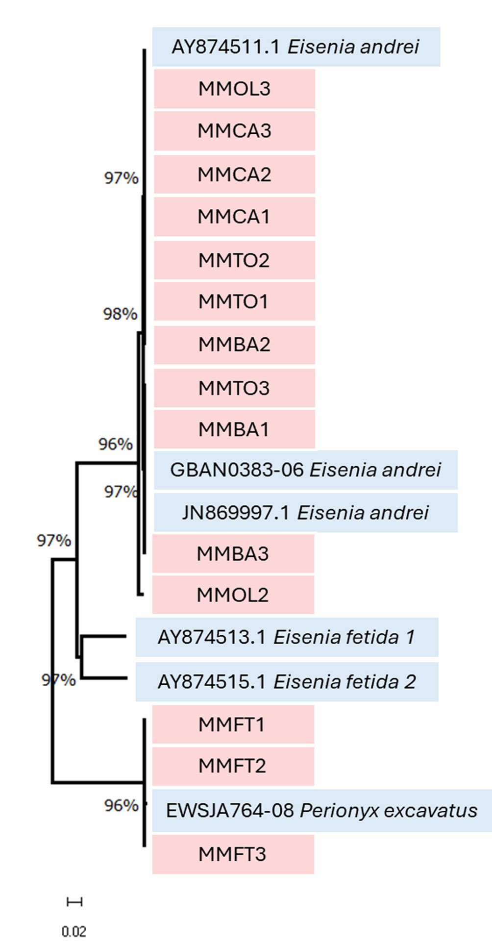
| Código de identificación | Origen | Secuencia 650-653 pb | BIN |
|---|---|---|---|
| TIAMD007-24 (MMCA1) | UNCADER | BOLD Systems | AAA8685 |
| TIAMD008-24 (MMCA42) | UNCADER | BOLD Systems | AAA8685 |
| TIAMD009-24 (MMCA3) | UNCADER | BOLD Systems | AAA8685 |
| TIAMD004-24 (MMTO1) | Teocelo | BOLD Systems | AAA8685 |
| TIAMD005-24 (MMTO3) | Teocelo | BOLD Systems | AAA8685 |
| TIAMD006-24 (MMTO5) | Teocelo | BOLD Systems | AAA8685 |
| TIAMD001-24 (MMFT1) | Tienda Hongos | BOLD Systems | AAC8637 |
| TIAMD002-24 (MMFT2) | Tienda Hongos | BOLD Systems | AAC8637 |
| TIAMD003-24 (MMFT3) | Tienda Hongos | BOLD Systems | AAC8637 |
| TIAMD010-24 (MMOL1) | Olmos | BOLD Systems | AAA8685 |
| TIAMD011-24 (MMOL2) | Olmos | BOLD Systems | AAA8685 |
| TIAMD012-24 (MMOL3) | Olmos | BOLD Systems | AAA8685 |
| TIAMD022-24 (MMBA1) | Rancho Balam | BOLD Systems | AAA8685 |
| TIAMD023-24 (MMBA2) | Rancho Balam | BOLD Systems | AAA8685 |
| TIAMD024-24 (MMBA3) | Rancho Balam | BOLD Systems | AAA8685 |
| AY874513.1 E. fetida | Römbke et al. (2016) | GenBank | — |
| AY874515.1 E. fetida | Römbke et al. (2016) | GenBank | — |
| JN869997.1 E. andrei | Römbke et al. (2016) | GenBank | — |
| GBAN0383-06 E. andrei | Römbke et al. (2016) | BOLD Systems | AAA8685 |
| AY874511.1 E. andrei | Römbke et al. (2016) | GenBank | — |
| EWSJA764-08 P. excavatus | Endemic Species Research Institute | BOLD Systems | AAC8637 |
Discusión
En el presente estudio, se empleó el análisis de código de barras de DNA (secuenciación del gen mitocondrial COI) para identificar las especies de lombrices de tierra presentes en 5 plantas de lombricompostaje. Cuatro plantas localizadas en la región de las altas montañas de Veracruz (MMTO, MMFT, MMCA y MMOL) y una en Playa del Carmen en Quintana Roo (MMBA). La evaluación de caracteres externos permitió identificar al menos 2 grupos morfológicamente distintos entre los ejemplares, posiblemente correspondientes a especies diferentes que, por sus características, podrían ser E. andrei y P. excavatus. De los 15 ejemplares evaluados, 12 provenientes de las plantas de lombricompostaje MMTO, MMCA, MMOL y MMBA compartieron un conjunto homogéneo de características morfológicas, mientras que los 3 individuos de la población MMFT presentaron un fenotipo claramente distinto. Para estudios futuros, se recomienda complementar la investigación con el análisis de caracteres internos y filogenias morfológicas, permitiendo una caracterización completa de las diferencias entre los grupos (Domínguez et al., 2015).
Para la identificación molecular, estudios previos han establecido umbrales de divergencia genética para la delimitación de especies mediante el gen COI. Hebert et al. (2003) encontraron que las divergencias de COI rara vez superan 2% dentro de una especie determinada, mientras que los miembros de especies diferentes suelen presentar divergencias mayores. Chang y James (2011) revisaron la literatura y concluyeron que divergencias inferiores a 9% pueden asignarse a la misma especie. En estudios previos con lombrices de tierra, Römbke et al. (2016) señalaron que valores superiores a 10% podrían indicar diferenciación entre especies. Chang et al. (2009) reportaron que las divergencias intraespecíficas en el gen COI en lombrices de tierra presentan un promedio de 1.3%, mientras que las diferencias interespecíficas alcanzan un promedio de 18.7%.
En nuestro análisis, las distancias genéticas calculadas entre los especímenes muestreados en las plantas de lombricompostaje MMTO, MMCA, MMBA, la secuencia MMOL3 de la planta MMOL y las secuencias de referencia de E. andrei fueron notablemente bajas (< 0.32%). La secuencia MMOL2 presentó una divergencia ligeramente mayor (entre 1.2 y 1.3%) con respecto a las secuencias de referencia de E. andrei; sin embargo, su divergencia genética no excede (2%) los límites típicos observados de variación intraespecífica (Chang et al., 2009). Además, la herramienta de identificación del sistema BOLD asignó a todas estas secuencias, incluida MMOL2, el BIN AAA8685, que coincide con E. andrei (tabla 2). Es importante destacar que no existe un umbral de divergencia genética fijo para determinar cuándo 2 muestras pertenecen a diferentes especies. Sin embargo, tomando en cuenta el patrón observado por Chang et al. (2009) en las divergencias intraespecíficas, indica que los ejemplares recolectados en las plantas de lombricompostaje MMCA, MMBA, MMTO y MMOL pertenecen a la especie E. andrei.
| P. excavatus EWSJA764-08 | E. andrei GBAN0383-06 | E. andrei JN869997.1 | E. andrei AY874511.1 | E. fetida AY874513.1 | E. fetida AY874515.1 | |
|---|---|---|---|---|---|---|
| MMFT1 | 0.0015409276 | 0.2629987796 | 0.2644016040 | 0.2653194932 | 0.2358330274 | 0.2363505591 |
| MMFT2 | 0.0015409276 | 0.2629987796 | 0.2644016040 | 0.2653194932 | 0.2358330274 | 0.2363505591 |
| MMFT3 | 0.0015409276 | 0.2629987796 | 0.2644016040 | 0.2653194932 | 0.2358330274 | 0.2363505591 |
| MMTO1 | 0.2671755709 | 0.0030865172 | 0.0032841858 | 0.0000000000 | 0.1649064730 | 0.1674082417 |
| MMTO2 | 0.2671755709 | 0.0030865172 | 0.0032841858 | 0.0000000000 | 0.1649064730 | 0.1674082417 |
| MMTO3 | 0.2648485363 | 0.0000000000 | 0.0000000000 | 0.0030865172 | 0.1649064730 | 0.1653642510 |
| MMCA1 | 0.2671755709 | 0.0030865172 | 0.0032841858 | 0.0000000000 | 0.1649064730 | 0.1674082417 |
| MMCA2 | 0.2671755709 | 0.0030865172 | 0.0032841858 | 0.0000000000 | 0.1649064730 | 0.1674082417 |
| MMCA3 | 0.2671755709 | 0.0030865172 | 0.0032841858 | 0.0000000000 | 0.1649064730 | 0.1674082417 |
| MMOL2 | 0.2558729431 | 0.0124453913 | 0.0132493333 | 0.0124453913 | 0.1708936388 | 0.1693152390 |
| MMOL3 | 0.2671755709 | 0.0030865172 | 0.0032841858 | 0.0000000000 | 0.1649064730 | 0.1674082417 |
| MMBA1 | 0.2648485363 | 0.0000000000 | 0.0000000000 | 0.0030865172 | 0.1649064730 | 0.1653642510 |
| MMBA2 | 0.2671755709 | 0.0030865172 | 0.0032841858 | 0.0000000000 | 0.1649064730 | 0.1674082417 |
| MMBA3 | 0.2650342592 | 0.0015402451 | 0.0000000000 | 0.0046315330 | 0.1647547930 | 0.1651978963 |
Por otro lado, las secuencias provenientes de la planta MMFT, mostraron una divergencia genética mínima (0.15%) con respecto a la secuencia de referencia de P. excavatus e identificadas como esta especie por BOLD Systems (BIN AAC8637). También, todas las secuencias estudiadas mostraron niveles de divergencia de entre 16 y 23% con respecto a E. fetida, lo que sugiere que ninguna de las secuencias analizadas pertenece a esta especie. Estos hallazgos contradicen las afirmaciones de los propietarios de las plantas de lombricompostaje, quienes indican que las lombrices composteras que cultivan corresponden a E. fetida. Sin embargo, diversas publicaciones sobre el tema señalan la presencia de E. andrei y P. excavatus en instalaciones similares (Aranda et al., 1999, 2011).
Asimismo, el análisis fenético basado en el método de NJ (fig. 1) permitió observar una clara agrupación de las secuencias obtenidas de las plantas MMCA, MMBA, MMTO con las secuencias de referencia de E. andrei. En el caso de la planta MMOL, la secuencia MMOL3, se agrupa consistentemente con el clado de las secuencias de E. andrei. Sin embargo, a pesar de haber sido recolectadas en el mismo sitio y pertenecer a la misma población cultivada, la secuencia MMOL2 se ubicó en una rama separada dentro del árbol fenético, en concordancia con los resultados obtenidos en la matriz de distancias genéticas por pares. Su ubicación en el árbol de NJ sugiere una posible diferenciación intraespecífica. Esta discrepancia puede atribuirse a las limitaciones del método fenético utilizado, el cual se basa únicamente en similitudes de distancia y no en relaciones filogenéticas estadísticamente robustas (Saitou y Nei, 1987). También es posible que MMOL2 represente un haplotipo divergente o una población estructurada genéticamente dentro de E. andrei. Este tipo de variación intraespecífica ha sido documentada previamente en lombrices de tierra cultivadas y no necesariamente implica diferenciación a nivel de especie (Chang et al., 2009). Sin embargo, para esclarecer esta posibilidad, sería recomendable integrar otros datos de secuencias mitocondriales como el 16S (Yadav y Mullah, 2017), secuencias nucleares (H3, ITS2, 18S, 28S) y de genotipado (microsatélites o SNPs) que ofrezcan mayor resolución (Barraux et al., 2024). Este hallazgo, también resalta la importancia de analizar múltiples individuos por sitio y no asumir homogeneidad genética dentro de una misma población cultivada.
Por otro lado, las secuencias de la planta MMFT se agruparon consistentemente con la secuencia de referencia de P. excavatus. Estas agrupaciones presentaron altos valores de soporte bootstrap, lo que respalda la solidez de las asignaciones taxonómicas basadas en el código de barras de DNA.
El análisis fenético basado en el método de NJ es una herramienta útil para la identificación molecular de lombrices de tierra, ya que permite visualizar agrupamientos basados en similitudes genéticas y evaluar la consistencia entre secuencias de prueba y secuencias de referencia. Aunque este enfoque no permite inferencias evolutivas profundas, brinda una delimitación rápida y confiable de especies, como en estudios ecológicos o de lombricompostaje, donde las especies pueden presentar morfologías crípticas (Chang et al., 2009; King et al., 2008). Este enfoque, combinado con el análisis de distancias génicas por pares ha sido validado como una estrategia eficaz para diferenciar especies dentro de géneros complejos como Eisenia, donde la identificación resulta limitada (Römbke et al., 2016). Aunque en este estudio no se secuenció el gen COI completo, la región utilizada (650-653 pb) corresponde al fragmento estandarizado para el código de barras en invertebrados y por su eficacia ha sido ampliamente validado en estudios previos (Hebert et al., 2003; Ratnasingham y Hebert, 2013).
La presencia de P. excavatus en una de las plantas de lombricompostaje resulta particularmente relevante en el ámbito de la ecología aplicada, debido a su elevada tasa de reproducción, rápida colonización del sustrato y amplia tolerancia ambiental (tabla 4) (Suthar y Singh, 2008). Su presencia indica su capacidad de adaptación a condiciones ambientales específicas en las plantas de lombricompostaje, donde los operadores asumían que las lombrices de tierra composteras que cultivan son E. fetida y/o roja californiana.
Por otro lado, E. andrei fue la especie predominante en la mayoría de las plantas analizadas. Su prevalencia se explica por sus características biológicas: distribución cosmopolita, ciclo de vida corto, amplia tolerancia a la variación climática, facilidad de manejo en entornos operativos y experimentales (tabla 4) (Domínguez y Edwards, 2004). Características biológicas que la han convertido en una de las especies más utilizadas en programas de lombricompostaje a nivel global (Domínguez y Edwards, 2004) y utilizada como especie centinela (al igual que E. fetida) en los estudios ecotoxicológicos ISO-17512 (ISO, 2008) y ISO-11268 (ISO, 2012).
En conclusión, el análisis de la región estándar del gen mitocondrial COI (DNA barcoding) permitió identificar con precisión 2 especies de lombrices de tierra composteras E. andrei y P. excavatus, descartando la presencia de E. fetida en las plantas de lombricompostaje evaluadas en las altas montañas del centro de Veracruz y el Caribe mexicano (Quintana Roo). La identificación molecular obtenida concuerda, en gran medida, con revisiones taxonómicas previas basadas en caracteres morfológicos, como las analizadas por Aranda et al. (1999) y Fragoso (2011), las cuales ya habían señalado la presencia predominante de E. andrei en sistemas de lombricompostaje y en tiraderos y cúmulos de pulpa de café del centro de Veracruz. Finalmente, la confirmación de E. andrei y P. excavatus como especies presentes en los sistemas evaluados sugiere la conveniencia de explorar su coexistencia y desempeño conjunto en procesos de lombricompostaje y biorremediación de materiales orgánicos, como el sargazo (Sargassum spp.), con el fin de optimizar la eficiencia biológica y ambiental de estos sistemas (Martínez-Cano et al., 2024).
| Especie | Familia | Origen biogeográfico | Estatus en México | Rango altitudinal (m snm) | Rango térmico (°C) | Presencia en México | Referencias |
|---|---|---|---|---|---|---|---|
| Eisenia andrei | Lumbricidae | Europa | Exótica | 800-2,500 | 10-25 | Sistemas de vermicompostaje o sitios artificiales | (Domínguez y Edwards, 2004; Fragoso, 2011; Fragoso y Rojas, 2014) |
| Perionyx excavatus | Megascolescidae | Asia | Exótica introducida/naturalizada | 0-800 | 20-35 | Suelos de plantaciones y ecosistemas perturbados | (Fragoso, 2011; Fragoso y Rojas, 2014; Suthar y Singh, 2008) |
Agradecimientos
Los autores agradecen a Alma Estrella García Morales por el procesamiento de las muestras de tejido para el análisis de DNA en el Laboratorio de Códigos de Barras de la Vida, Nodo Chetumal. Asimismo, agradecen a los propietarios de las plantas de lombricompostaje por la donación del material biológico. Mayela Martínez Cano agradece al Secihti por la beca de doctorado (1129824).
Referencias
Aranda, E. y Barois, I. (2000). Coffee pulp vermicomposting treatment. En T. Sera, C. R. Soccol, A. Pandey y S. Roussos (Eds.), Coffee biotechnology and quality (pp. 489–506). identificadas en las plantas de lombricompostaje de Veracruz Rango Presencia en Referencias altitudinal térmico México snm) (ºC) 800-2,500 10-25 Sistemas de (Domínguez y vermicompostaje o Edwards, 2004; sitios artificiales Fragoso, 2011; Fragoso y Rojas, 2014) 20-35 Suelos de (Fragoso, 2011; plantaciones Fragoso y Rojas, 2014; y ecosistemas Suthar y Singh, 2008) perturbados Dordrecht: Kluwer Academic Publishers. https://doi.org/10.1007/978-94-017-1068-8_46
Aranda, E., Barois, I., Arellano, P., Irissón, S., Salazar, T., Rodríguez, J. et al. (1999). Vermicomposting in the Tropics. En P. Lavelle, L. Brussaard y P. Hendrix (Eds.), Earthworm management in tropical agroecosystems (pp. 253–287). Wallingford, United Kingdom: CABI Publishing.
Aranda, E., Barois I., Santos, B. M. y Hernandez-Castellanos, B. (2011). Vermicomposting, research and activities in Mexico. En C. A. Edwards, N. Q. Arancon y R. L. Sherman (Eds.), Vermiculture technology: earthworms, organic wastes, and environmental management (pp. 507–32). Boca Raton, Florida: CRC Press.
Barraux, A., Noël, S., Roy, V. y Dupont, L. (2024). Challenges of molecular barcode-based identification of earthworm specimens for biodiversity assessment. Frontiers in Ecology and Evolution, 12, 1358984. https://doi.org/10.3389/fevo.2024.1358984
Chang, C. H. y James, S. (2011). A critique of earthworm molecular phylogenetics. Pedobiologia, 54, S3–S9. https://doi.org/10.1016/j.pedobi.2011.07.015
Chang, C. H., Rougerie, R. y Chen, J. H. (2009). Identifying earthworms through DNA barcodes: pitfalls and promise. Pedobiologia, 52, 171–80. https://doi.org/10.1016/j.pedobi.2008.08.002
de Waard, J., Ivanova, N., Hajibabaei, M. y Hebert, P. (2008). Assembling DNA barcodes: analytical protocols. En C. C. Martin (Ed.), Methods in Molecular Biology: environmental genomics methods (pp. 275–294). Ottawa: Humana Press https://doi.org/10.1007/978-1-59745-548-0_15
Domínguez, J., Aira, M., Breinholt, J. W., Stojanovic, M., James S. W. y Pérez-Losada, M. (2015). Underground evolution: new roots for the old tree of lumbricid earthworms. Molecular Phylogenetics and Evolution, 83, 7–19. https://doi.org/10.1016/j.ympev.2014.10.024
Domínguez, J. y Edwards, C. A. (2004). Vermicomposting organic wastes: a review. Soil Zoology for Sustainable Development in the 21st Century. Cairo: Geocites Publisher.
Domínguez, J. y Pérez-Losada, M. (2010). Eisenia fetida (Savigny, 1826) y Eisenia andrei Bouché, 1972 son dos especies diferentes de lombrices de tierra. Acta Zoológica Mexicana, 26, 321–31. https://doi.org/10.21829/azm.2010.262897
Domínguez, J., Velando A. y Ferreiro, A. (2005). Are Eisenia fetida (Savigny, 1826) and Eisenia andrei Bouché (1972) different biological species? Pedobiologia, 49, 81–87. https://doi.org/10.1016/j.pedobi.2004.08.005
Fragoso, C. (2011). Lombrices de tierra (Annelida: Oligochaeta). La biodiversidad en Veracruz: estudio de estado (pp. 259– 268). México D.F.: Comisión Nacional para el Conocimiento y Uso de la Biodiversidad/ Gobierno del Estado de Veracruz/ Universidad Veracruzana/ Instituto de Ecología A.C.
Fragoso, C. y Rojas, P. (2014). Biodiversidad de lombrices de tierra (Annelida: Oligochaeta: Crassiclitellata) en México. Revista Mexicana de Biodiversidad, 85 (Suplem.), 197–207. https://doi.org/10.7550/rmb.33581
García, S. R., Méndez, G., Velázquez, M. G., Castillo, G. y Retureta, A. (2019). Dinámica poblacional de Eisenia fetida (Savigny, 1826) y Eisenia andrei (Bouché, 1972) en tres sustratos diferentes. Revista Biológico Agropecuaria Tuxpan, 7, 70–78. https://doi.org/10.47808/revistabioagro.v7i2.31
Hebert, P. D. N., Cywinska, A., Ball, S. L. y deWaard, J.R. (2003). Biological identifications through DNA barcodes. Proceedings of the Royal Society B: Biological Sciences, 270, 313–321. https://doi.org/10.1098/rspb.2002.2218
ISO (International Organization for Standardization). (2008). Soil quality: avoidance test for determining the quality of soils and effects of chemicals on behavior. ISO 17512-1. International Organization for Standardization. Disponible en: https://www.iso.org/obp/ui/en/#iso:std:iso:17512:-1:ed-1:v1:en
ISO (International Organization for Standardization). (2012). Soil quality: effects of pollutants on earthworms. ISO 11268-1. International Organization for Standar- dization. Disponible en: https://www.iso.org/obp/ui/#iso:std:iso:11268:-1:ed-2:v1:en
ISO (International Organization for Standardization). (2019). Soil quality: identification of ecotoxicological test species by DNA barcoding. ISO 21286. International Organization for Standardization. Disponible en: https://www.iso.org/obp/ui/en/#iso:std:iso:21286:ed-1:v1:en
James, S. W., Porco D., Decaëns, T., Richard, B., Rougerie, R. y Erséus, C. (2010). DNA Barcoding reveals cryptic diversity in Lumbricus terrestris L., 1758 (Clitellata): resurrection of L. herculeus (Savigny, 1826). Plos One, 5, 1–8. https://doi.org/10.1371/journal.pone.0015629
King, R. A., Tibble, A. L. y Symondson, W. O. C. (2008). Opening a can of worms: unprecedented sympatric cryptic diversity within British lumbricid earthworms. Molecular Ecology, 17, 4684–4698. https://doi.org/10.1111/j.1365-294X.2008.03931.x
Kumar, S., Stecher, G. y Tamura, K. (2016). MEGA7: molecular evolutionary genetics analysis version 7.0 for bigger datasets. Molecular Biology and Evolution, 33, 1870–1874. https://doi.org/10.1093/molbev/msw054
Martínez-Cano, M., Dorantes-Acosta, A. E., Lara-González, R., Salgado-Hernández, E. y Ortiz-Ceballos, A. I. (2024). Effect of sargassum on the behavior and survival of the earthworm Eisenia fetida. Bulletin of Environmental Contamination and Toxicology, 113, 36. https://doi.org/10.1007/s00128-024-03935-5
Montero-Pau, J., Gómez, A. y Muñoz, J. (2008). Application of an inexpensive and high-throughput genomic DNA extraction method for the molecular ecology of zooplanktonic diapausing eggs. Limnology and Oceanography: Methods, 6, 218–222. https://doi.org/10.4319/lom.2008.6.218
Moreno, A. G. y Borges, S. (2004). Advances in earthworm taxonomy. Madrid: Editorial Complutense.
Prosser, S., Martínez-Arce, A. y Elías-Gutiérrez, M. (2013). A new set of primers for COI amplification from freshwater microcrustaceans. Molecular Ecology Resources, 13, 1151– 1155. https://doi.org/10.1111/1755-0998.12132
Ratnasingham, S. y Hebert, P. D. N. (2013). A DNA-based registry for all animal species: The Barcode Index Number (BIN) System. Plos One, 8, e66213. https://doi.org/10.1371/journal.pone.0066213
Römbke, J., Aira, M., Backeljau, T., Breugelmans, K., Domínguez, J., Funke, E. et al. (2016). DNA barcoding of earthworms (Eisenia fetida/andrei complex) from 28 ecotoxicological test laboratories. Applied Soil Ecology, 104, 3–11. https://doi.org/10.1016/j.apsoil.2015.02.010
Saitou, N. y Nei, M. (1987). The neighbor-joining method: a new method for reconstructing phylogenetic trees. Molecular Biology and Evolution, 4, 406–425. https://doi.org/10.1093/oxfordjournals.molbev.a040454
Suthar, S. y Singh, S. (2008). Vermicomposting of domestic waste by using two epigeic earthworms (Perionyx excavatus and Perionyx sansibaricus). International Journal of Environmental Science & Technology, 5, 99–106. https://doi.org/10.1007/BF03326002
Yadav, S. y Mullah, M. (2017). A review on molecular markers as tools to study earthworm diversity. International Journal of Pure and Applied Zoology, 5, 62–69.
Zhang, M., Jouquet, P., Dai, J., Xiao, L., Du, Y., Liu, K. et al. (2022). Assessment of bioremediation potential of metal contaminated soils (Cu, Cd, Pb and Zn) by earthworms from their tolerance, accumulation and impact on metal activation and soil quality: a case study in South China. Science of The Total Environment, 820, 152834. https://doi.org/10.1016/j.scitotenv.2021.152834

Evolución

Biogeografía

Notas científicas
Notas científicas