Oak Origins: From Acorns to Species and the Tree of Life, published in December 2024, is Andrew Hipp’s most recent book. Portraying oaks as a doorway to understanding the rest of organisms and using data on their history, present and future, he guides us to comprehend evolutionary mechanisms at all levels, lean out on the surprising interconnections of the web of life and, ultimately, to have a glimpse of our own -human beings- future.
Combining rigorously written science with a sensory imagination, Hipp makes you feel immersed, witnessing events, places and ages in total wonder and delight. Through these journeys, the scientific interest in evolution, genomics, phylogeny, systematics or ecology becomes one with the passionate naturalist in all of us.
The book is illustrated by the fine art of Rachel D. Davis with 43 mid-tones watercolor and opens through a charming foreword by Béatrice Chassé. Enjoyable from the first to the last sentence, this is already a jewel of the science popularization in Biology.
Warning: better to refrain from marking texts or bookmarking pages because when you see the next part you feel tempted to mark it too, and the rest, and the rest…
Dr. Andrew Hipp is a scientist, writer and science communicator. He is the Herbarium Director and senior scientist in the Morton Arboretum, where he directs research on the systematics, evolution and ecological implications of plant diversity. He is also a lecturer at the University of Chicago. He has published more than 130 scientific papers and chapter books, 16 children´s books, and communicate through workshops and his blog A Botanist’s Field Notes.
The content of the book is as follows: Foreword: Figuring things out, by Béatrice Chassé; Introduction: What is an oak? Chapter 1. Flowers and acorns: populations arise and migrate; Chapter 2. Variation: populations evolve; Chapter 3. Species and their hybrids; Chapter 4. Origins: Fagaceae; Chapter 5. Radiation: Quercus; Chapter 6. “Pharaoh’s Dance”: The oak genome; Chapter 7. Oak communities; Epilogue: The future of oaks; Acknowledgments; Appendix: Oak names.
Alejandro Lizama-Hernández a, Ma Ventura Rosas-Echeverría a, *, M. Guadalupe del Rio b
a Universidad Autónoma del Estado de Morelos, Escuela de Estudios Superiores del Jicarero, Laboratorio de Sistemática y Evolución de Insectos, Carretera Galeana-Tequesquitengo s/n, Colonia El Jicarero, 62909 Jojutla, Morelos
b Museo de La Plata, División Entomología- Consejo Nacional de Investigaciones Científicas y Técnicas, Paseo del Bosque s/n, 1900 La Plata, Buenos Aires, Argentina
Received: 01 October 2024; accepted: 27 January 2025
Abstract
The first phylogenetic analysis of the weevil genus Megalostylus endemic to Mexico(Entiminae, Naupactini) is presented, based on a data matrix of 37 morphological characters of adults and 21 terminal taxa. The ingroup comprises 9 species, 4 varieties, and 5 specimens of Megalostylus whose identification at the species level is doubtful. The outgroup includes species representing closely related genera: Pantomorus albosignatus, Naupactus cervinus, and Megalostylodes hirsutus. The objectives were to test the monophyly of Megalostylus, to explore its species relationships, and to determine which synapomorphies allow its identification and differentiation from other genera. The analysis yielded a single cladogram of 61 steps, showing the following phylogenetic sequence: (Pantomorusalbosignatus (Naupactus cervinus (Megalostylodeshirsutus (Megalostylus rhodopus (M. morpho 2(M. macrophthalmus (M. tomentosus (M. dilaticollis (M. albicans (M. brevipilis, M. fusiformis (M. splendidus – M. sturmi))))))))))).The results support the monophyly of Megalostylus based on the following synapomorphies: protibia with a prominence opposite to mucro, elytra almost flat, sternite VIII subrhomboidal very elongated, and aedeagus smooth. They also support its sister-group relationship with Megalostylodes.
Keywords: Systematics; Naupactini; Morphology; New species; New varieties; Megalostylodes
Filogenia del género de gorgojos Megalostylus (Coleoptera: Curculionidae: Entiminae), endémico de México
Resumen
Presentamos el primer análisis filogenético del género de gorgojos Megalostylus endémico de México(Entiminae, Naupactini)basado en una matriz de datos de 37 caracteres morfológicos de adultos y 21 taxones terminales. El grupo interno comprende 9 especies, 4 variedades y 5 especímenes de Megalostylus de dudosa identificación a nivel de especie. El grupo externo está formado por 3 especies representantes de géneros relacionados cercanamente: Pantomorus albosignatus, Naupactus cervinus y Megalostylodes hirsutus. Los objetivos fueron poner a prueba la monofilia de Megalostylus, explorar sus relaciones interespecíficas y determinar qué sinapomorfías lo identifican y diferencian de otros géneros. El análisis produjo un solo cladograma de 61 pasos, que muestra la siguiente secuencia filogenética: (Pantomorusalbosignatus (Naupactus cervinus (Megalostylodeshirsutus (Megalostylus rhodopus (M. morpho 2(M. macrophthalmus (M. tomentosus (M. dilaticollis (M. albicans (M. brevipilis, M. fusiformis (M. splendidus – M. sturmi))))))))))). Los resultados avalan la monofilia de Megalostylus con base en las siguientes sinapomorfías: protibias con una prominencia opuesta al mucro, élitros casi planos en vista lateral, esternito VIII subromboidal muy elongado y aedeago liso. También respaldan su estrecha relación con Megalostylodes.
Palabras clave: Sistemática; Naupactini; Morfología; Especie nueva; Variedades nuevas; Megalostylodes
Introduction
Megalostylus Schoenherr, 1840 (Entiminae, Naupactini) is a genus of broad-nosed weevils distributed in the Mexican states of Durango, Guanajuato, Guerrero, Michoacán, Morelos, Oaxaca, Puebla and Veracruz (Champion, 1911; Muñiz-Vélez et al., 2015; Ordóñez- Reséndiz et al., 2008). It was described by Schoenherr (1840) in his monumental work Genera et species curculionidum, cum synonymia hujus familiae, specie novae aut hactenus minus cognitae based on the type species M. sturmi Boheman, 1840 and has been traditionally characterized by the presence of a short antennal scape comparatively stouter at apex than in other genera (Champion, 1911; Figs. 1-3). The most complete treatment of Megalostylus was conducted by Champion (1911), who recognized 9 species and assigned this genus to “Otiorhynchinaealatae”, group “Cyphina”. He also provided a taxonomic key based on 32 morphological characters of adults and the complete distribution records of the species until then.
The classification of Megalostylus proposed by Champion (1911) more than a century ago needs a revision of the status of the species, the infraspecific varieties, and a phylogenetic analysis, to test the monophyly, species relationships, and synapomorphies that support the genus.
Materials and methods
We examined 347 adult specimens obtained from the following entomological collections: IBUNAM, Instituto de Biología, Universidad Nacional Autónoma de México, Mexico City, Mexico; INECOL, Instituto de Ecología, A. C., Xalapa, Veracruz, Mexico; USNM, National Museum of Natural History, Washington DC, USA; NHRS, Swedish Museum of Natural History, Stockholm, Sweden; and BMNH, Natural History Museum, London, England. Moreover, we included material collected by the working team at the Laboratorio de Sistemática y Evolución de Insectos (LabSei) of the ESSJicarero, UAEM.
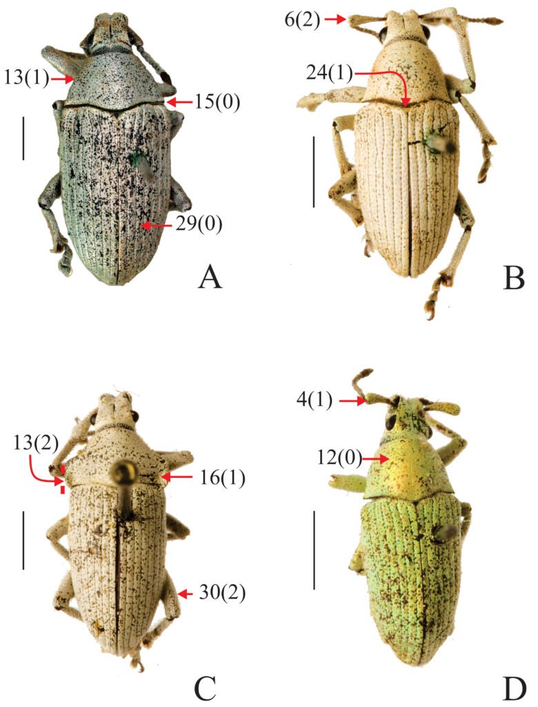
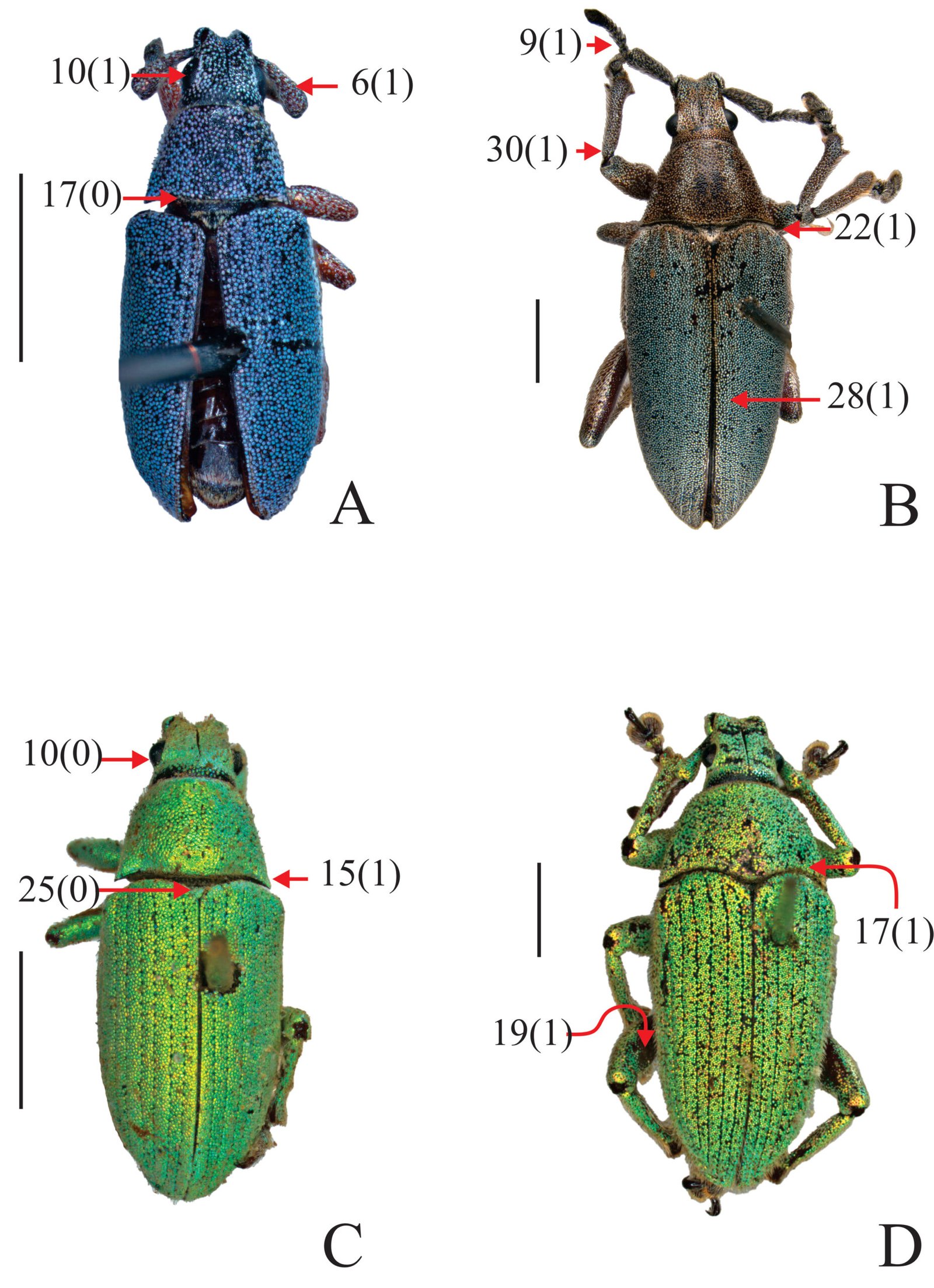
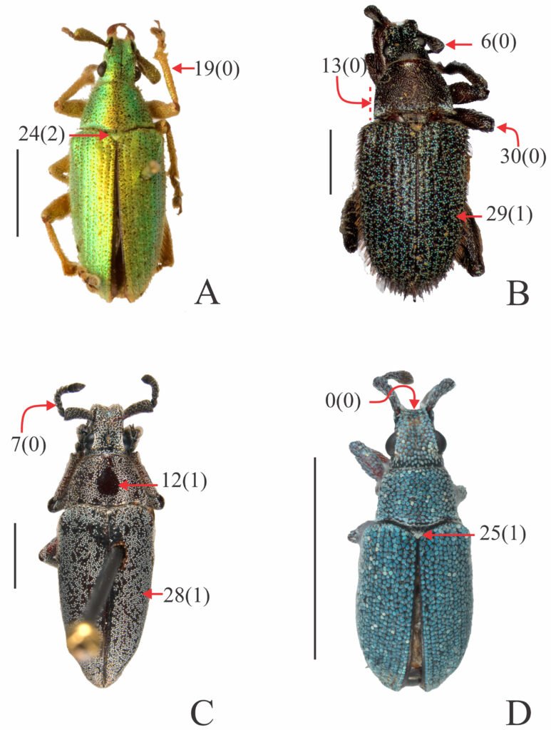
Taxon sampling. The outgroup comprises 3 species: Megalostylodes hirsutus Champion, 1911, Naupactus cervinus (Boheman, 1840), and Pantomorus albosignatus Boheman, 1840, the former representing the most closely related genus. The ingroup includes 9 species (Figs. 1-3): M. sturmi Boheman,1840, M. rhodopus Boheman, 1840, M. albicans (Lacordaire, 1876), M. splendidus Chevrolat, 1878, M. brevipilis Champion, 1911, M. dilaticollis Champion, 1911, M. fusiformis Champion, 1911, M. macrophthalmus Champion, 1911, and M. tomentosus Champion, 1911 (Table 1). Additionally, 4 described varieties and 5 specimens of doubtful identification at species-level were included as morphospecies1-5.
A list of 37 discrete characters (29 binary and 8 multistate) was recorded from adults, including 33 characters from the external morphology, 2 of the female genitalia, and 2 of the male genitalia (Table 2). The selection of characters was based on previous analyses of the tribe Naupactini (del Río, 2009; Lanteri & del Río, 2017; Rosas et al., 2011).
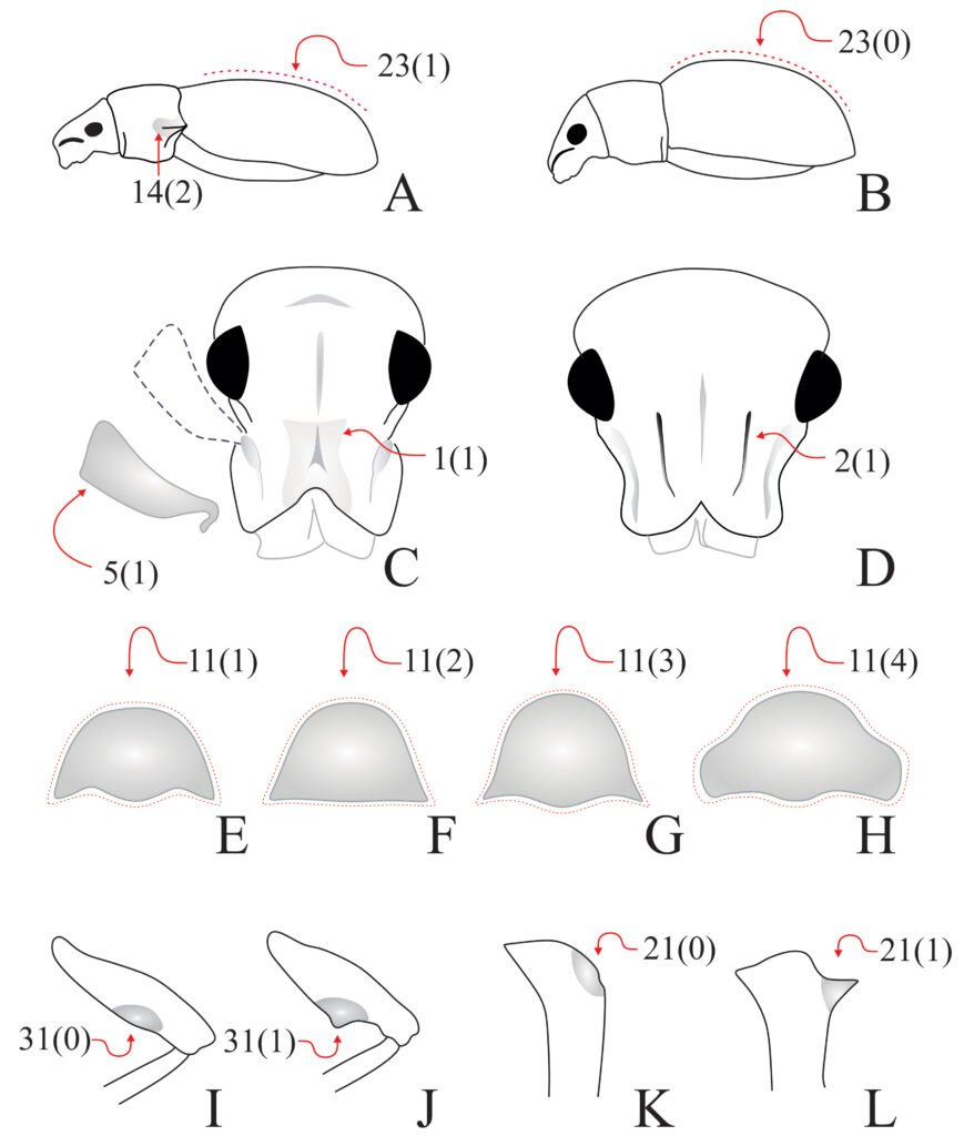
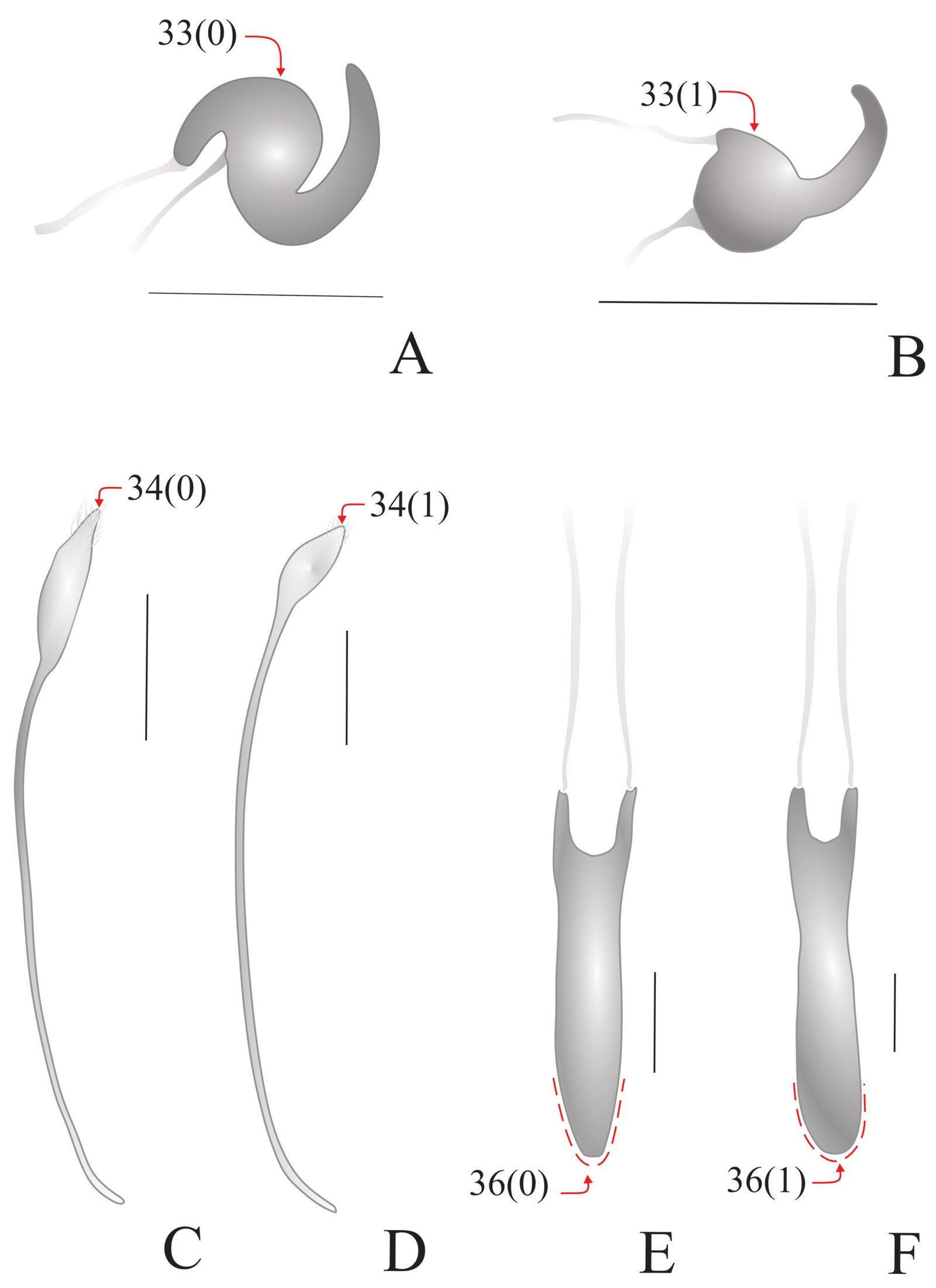
For the preparation of genital structures, we followed the methodology described in Rosas et al. (2011) and Lanteri and del Río (2017). A Carl Zeiss Stemi 2000 stereomicroscope, equipped with a reticle eyepiece was used for observations and measurements of the external and internal morphology. Photographs were taken with a Nikon D750 camera equipped with a SIGMA 150 mm 1:2.8 (macro) lens, and drawings were made with Corel Draw (2020 version 22.0.0412). Most characters were illustrated by photographs and drawings, to facilitate the recognition of character states (Figs. 4, 5). They were highlighted with arrows, with indication of character numbers and character states between parentheses.
Figure 1. Habitus photographs of Megalostylus species, dorsal view. A) Megalostylus albicans, female; B) M. brevipilis, male; C) M. dilaticollis, male; D) M. fusiformis male. Arrows and numbers indicate character codification, and the character state is indicated between parentheses. Scale bars = 2 mm.
A data matrix of 21 terminal groups and 37 morphological characters was compiled (Table 3). Character states that could not be examined (due to insufficient material) were scored with a “?” and character states with inapplicable entries on various terminals were scored with a “–”. Species or varieties showing 2 or more characters were coded as polymorphic characters. To facilitate the coding, Mesquite software version 3.70 was used (Maddison & Maddison, 2021). An implicit enumeration search was performed in the program TNT version 1.5 (Goloboff & Catalano, 2016). The characters were treated as unordered or non-additive, and under equal weights. The species Pantomorus albosignatus was used to root the trees. To evaluate branch support (BS), a standard Bootstrap with 1000 replicates was calculated in TNT. Branch support values greater than 50 were mapped in the cladogram. The resulting cladogram and character state transformations were examined in WINCLADA under fast optimization. All records were georeferenced, and maps created in ArcMap version 10. 4.1 (ESRI, 2015).
Figure 2. Habitus photographs of Megalostylus species, dorsal view. A) Megalostylus macrophthalmus, male; B) M. rhodopus, male; C) M. splendidus, male; D) M. sturmi, male. Arrows and numbers indicate character codification, the character state is indicated between parentheses. Scale bars = 2 mm.
Results
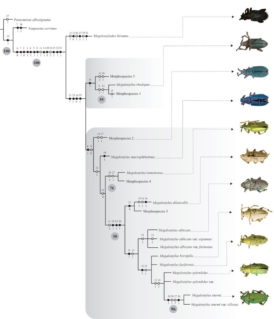
The search for the most parsimonious trees under equal weights yielded one most parsimonious tree (Fig. 6) (L = 63, IC = 0.73, IR = 0.83), showing the following phylogenetic sequence: (Pantomorus albosignatus (Naupactus cervinus (Megalostylodes hirsutus (Megalostylus)))).
Megalostylodes was found to be sister to the genus Megalostylus based on 12 synapomorphies: epistome scales similar in size, density, and color to those on the rest of the rostrum (0:0), dorsal surface of rostrum slightly to strongly depressed (1:1), absence of pair of dorsolateral carinae (2:0), scape very wide in males and thin in females (3:1), width of scape at apex greater than club width in males (4:1), shape of scape strongly clavate (5:1), color brown to black of the verticillate setae of funicle (9:1), slight lateral projection of pronotum (14:1), absence of a row of denticles on inner margin of protibia (20:0), vestiture of scutellum present, consisting of white scales or seta-like scales (25:1), presence of medial longitudinal depression of ventrites 1 and 2 on males (32:1), and subspherical body shape of spermatheca (33:1). There are also 2 homoplastic characters that support this relationship: pronotum subconical, with sides curved and strongly divergent from apex to base (11:1) and width of base of scutellum wider than interestria 2 (24:2).
Figure 3. Habitus photographs of Megalostylus species, dorsal view. A) Megalostylus tomentosus, male; B) Megalostylodes hirsutus, male; C) morphospecies 1, male; D) morphospecies 2, male. Arrows and numbers indicate character codification, the character state is indicated between parentheses. Scale bars = 2 mm.
Megalostylus was recovered as monophyletic based on 4 synapomorphies: presence of prominence opposite to mucro in protibia (21:1), elytra in lateral view almost flat (23:1), plate of sternite VIII, subrhomboidal very elongated (34:0), and sculpture of aedeagus smooth (35:1).
The sister genus Megalostylodes is characterized by 3 autapomorphies: pronotum narrower with respect to elytral base (13:0), very long elytral setae, longer than width of elytral interstriae 2 at middle (27:2), and presence of deeply excavated metafemur near apex (31:1), and 3 non-exclusive synapomorphies: presence of glabrous areas in midline of pronotum (12:1), erect disposition of elytral setae (26:1), and slightly convex interestriae (29:1).
Table 1
List of species included in the cladistic analysis of the genus Megalostylus and their geographic distributions (countries and states).
Species names
Geographic distributions
Pantomorus albosignatus Boheman
Mexico (Aguascalientes, Chihuahua, Coahuila, Mexico City, Durango, Guanajuato, Guerrero, Hidalgo, Monterrey, Oaxaca, Puebla Querétaro, San Luis Potosí, Veracruz, Zacatecas)
Naupactus cervinus (Boheman)
Argentina (Buenos Aires, Catamarca, Córdoba, Corrientes, Entre Ríos, Jujuy, Mendoza, Misiones, Salta, Santa Fe, Tucumán), Brasil (Paraná, Río Grande do Sul, Santa Catarina, São Paulo), México (Distrito federal), Uruguay (Artigas, Canelones, Colina, Durazno, Maldonado, Montevideo, Rio Negro, Treinta y Tres)
Megalostylodes hirsutus Champion
Mexico (Oaxaca)
Megalostylus albicans (Lacordaire)
Mexico (Colima, Estado de México, Guanajuato, Guerrero, Jalisco, Michoacán, Morelos, Nayarit, Oaxaca, Puebla)
Megalostylus brevipilis Champion
Mexico (Colima, Guerrero, Oaxaca)
Megalostylus dilaticollis Champion
Mexico (Guerrero, Michoacán, Morelos, Jalisco)
Megalostylus fusiformis Champion
Mexico (Morelos, Guerrero)
Megalostylus macrophthalmus Champion
Mexico (Oaxaca)
Megalostylus rhodopus Boheman
Mexico (Oaxaca)
Megalostylus splendidus Chevrolat
Mexico (Durango, Guerrero, Morelos, Puebla)
Megalostylus sturmi Boheman
Mexico (Guerrero, Michoacán)
Megalostylus tomentosus Champion
Mexico (Oaxaca)
Table 2
List of 37 morphological characters, character states and codes.
Character
Character states
0. Shape, size, density and color of epistome scales compared to those on the rest of the rostrum
Similar in size, density and color (0); smaller, scarcer and generally different in color (1)
1. Dorsal surface of rostrum
Flat (0); slightly to strongly depressed (1)
2. Pair of dorsolateral carinae
Absent (0); present (1)
3. Sexual dimorphism in antennae
Scape width subequal in males and females (0); scape very wide in males and thin in females (1)
4. Width of scape at apex with respect to width of club, in males
Less than club width (0); greater than club width (1)
5. Shape of scape
Capitate (0); strongly clavate (1)
6. Vestiture of scape
Absent to almost absent (0); scales dispersed leaving integument exposed (1); dense, space between scales reduced or absent, not leaving integument exposed (2)
7. Length of funicular antennomeres 1 and 2
Antennomere 2 slightly shorter than 1 or both sub-equal (0); antennomere 2 longer than 1 (1)
8. Antennae, scales on funicular antennomere 2
Absent (0); present (1)
9. Color of verticillate setae of funicle
Whitish or golden (0); brown to black (1)
10. Convexity of eyes
Convex, pronounced curvature, hemispherical shape (0); slightly convex, less pronounced curvature, small elevations (1)
Table 2. Continued
11. Shape of pronotum
Subcylindrical, curved sides and maximum width about half (0); subconical, with sides moderately to strongly curved and strongly divergent from apex to base (1); subconical, with sides slightly curved to straight and strongly divergent from apex to base (2); bell-shaped (3); subtrapezoidal, with sides slightly concave at anterior half and progressively expanding towards lateral sides at posterior half (4)
12. Glabrous areas at midline of pronotum
Absent (0); present (1)
13. Width of pronotum with respect to elytral base
Narrower (0); subequal (1); wider (2)
14. Lateral projection of pronotum
Absent or indistinct (0); slightly projected (1); strongly projected (2)
15. Shape of lateral projections of posterior margin of pronotum
Extended towards sides (0); strongly extended backwards, towards elytral base (1)
16. Sides at basal third of pronotum
Not depressed (0); strongly depressed (1)
17. Shape of posterior margin of pronotum
Straight to slightly bisinuate (0); strongly bisinuate (1)
18. Bulging surface beneath intercoxal granule, at anterior margin of prothorax
Indistinct or absent (0); present (1)
19. Color of legs integument
Light tones, reddish or orange (0); dark tones, black or brown (1)
20. Row of denticles on inner margin of protibia
Absent (0); present (1)
21. Prominence opposite to mucro in protibia
Absent (0); present (1)
22. Elytral anterior margin
Straight (0); bisinuate (1)
23. Shape of elytra in lateral view
Moderately convex (0); almost flat (1)
24. Width of base of scutellum with respect to width of interstria 2
Reduced to indistinct (0); subequal to width of interstria 2 (1); wider than interstria 2 (2)
25. Scutellum vestiture
Scales similar in color to those covering whole surface of elytra (0); Scales similar, consisted of white scales or seta-like scales (1)
26. Disposition of elytral setae
Recumbent to suberect (0); erect (1)
27. Size of elytral setae
Short (0); long, almost as long as width of interstria 2 at middle (1); very long, longer than width of elytral interestriae 2 at middle (2)
28. Arrangement of elytral setae
Uniform throughout elytral disc (0); only on lateral edges of elytral disc, dorsally without setae (1)
29. Convexity of interstriae
Flat (0); slightly convex (1)
30. Vestiture on legs
Absent or almost absent (0); inconspicuous, scales are scattered leaving integument exposed (1); conspicuous, space between scales is reduced or absent, and covered the integument (2)
31. Deep excavation on metafemur, near apex
Absent (0); present (1)
32. Medial longitudinal depression of ventrites 1 and 2, on males
Indistinct or absent (0); present (1)
33. Spermatheca, body shape
Subcylindrical, slender (almost as wide as base of cornu) (0); subspherical (1)
34. Shape of plate of sternite VIII
Subrhomboidal very elongated, with basal part much longer than apical part (0); subrhomboidal slightly elongated, with basal part as long as apical part (1)
35. Aedeagus, sculpture of median lobe
Granulose (0); smooth (1)
36. Aedeagus, shape of apex of median lobe
Acute to slightly acute (0); truncated (1); arrow shape (2)
Table 3
Data matrix of 21 taxa and 37 morphological characters of Megalostylus and outgroups used for the cladistic analysis. Inapplicable characters are indicated with a dash (-), and missing characters with a question mark (?).
Taxa
Characters
0-4
5-9
10-14
15-19
20-24
25-29
30-36
Pantomorus albosignatus
101?0
00000
00010
00000
10000
-0100
00?01??
Naupactus cervinus
10100
00100
00010
00000
10100
00000
00001?2
Megalostylodes hirsutus
01011
10001
01101
00000
00102
11201
0111100
Megalostylus albicans
01011
12010
02012
00101
01111
00000
1011010
Megalostylus albicans var. expansus
01011
12010
02022
00101
01111
00000
101??10
Megalostylus albicans var. farinosus
01011
120?0
02012
00101
01111
00000
101????
Megalostylus brevipilis
010?1
120?0
03011
10101
01111
00000
101??10
Megalostylus dilaticollis
01011
12000
04022
01001
01111
00000
10110??
Megalostylus fusiformis
010?1
120?0
03011
10101
01111
00000
10?????
Megalostylus macrophthalmus
01011
100?
12011
00000
01112
10000
00?10??
Megalostylus splendidus
01011
12010
01011
10101
01112
00000
1011010
Megalostylus splendidus var.
01011
12010
01011
10101
01112
00000
1011010
Megalostylus sturmi
01011
12010
0100&11
10111
01112
01100
1011?11
Megalostylus sturmi var. villosus
01011
12010
0100&11
10111
01112
01100
1011011
Megalostylus rhodopus
01011
12001
01111
00000
01112
10010
0011010
Megalostylus tomentosus
01011
110?0
02011
00000
01112
01100
00110??
Morphospecies 1
010?1
12001
01111
10000
0111?
10010
001??10
Morphospecies 2
010?1
11000
01011
10100
01112
10000
001??10
Morphospecies 3
010?1
10001
02011
00000
01112
10011
001??10
Morphospecies 4
010??
11000
02011
00000
01112
01100
00?10??
Morphospecies 5
010?1
12000
04011
00001
01111
00000
101??10
Two main clades were found within Megalostylus: clade I, including Megalostylus rhodopus and morphospecies 1 and 3 (considered belonging to M. rhodopus), is supported by 1 exclusive synapomorphy: elytral setae only present on the lateral edges of elytral disc (28:1). Clade II is supported by 1 exclusive synapomorphy and 1 non-exclusive synapomorphy: scales of scape separate, leaving integument exposed (6:1) and whitish or golden color of the verticillate setae of funicle (9:0), respectively. Within clade II, morphospecies2 is sister to the remaining species, which form a clade supported by 1 non-exclusive synapomorphy: pronotum subconical, sides slightly curved to straight and strongly divergent from apex to base (11:2). Megalostylus macrophthalmus is the sister species of M. tomentosus–M. sturmi var. villosus based on 1 non-exclusive synapomorphy: vestiture of scutellum present, scales similar in color to those covering the whole surface of elytra (25:0). Megalostylus tomentosus (along with morphospecies4) is the sister of a supported clade (BT 58) M. dilaticollis–M. sturmi var. villosus clade, which is supported by 3 exclusive synapomorphies and 1 non-exclusive synapomorphy: integument of legs with dark tones, black or brown (19:1), and width of base of scutellum reduced to indistinct (24:1), vestiture on legs inconspicuous, scales are scattered leaving integument exposed (30:1), and scales separated leaving integument of scape exposed (6:2). Within this clade M. dilaticollis (along with morphospecies 5) is sister to a subclade supported by 1 exclusive synapomorphy and 1 non-exclusive synapomorphy: presence of scales on the second funicular antennomere (8:1) and posterior margin of pronotum strongly bisinuate (17:1) that includes M. albicans and its varieties, M. albicans var. expansus, and var. farinosus sister to M. brevipilis to M. sturmi var. villosus clade supported by 1 exclusive synapomorphy and 1 non-exclusive synapomorphy: pronotum flared or bell-shaped (11:3) and lateral projections of posterior margin of pronotum strongly extended backward, towards elytral base (15:1). Within this clade, M. brevipilis and M. fusiformis are sisters to the M. splendidus–M. sturmi var. villosus clade which is supported by 2 non-exclusive synapomorphies: pronotum subconical, sides curved and strongly divergent from apex to base (11:1), and width of base of scutellum wider than interestria 2 (24:2). The clade M. splendidus–M. sturmi var. villosus also has unresolved relationships between M. splendidus and his variety, both sister to the M. sturmi + M. sturmi var. villosus clade.
Figure 4. Diagrammatic illustrations with arrows and numbers indicating character codification of head, pronotum, legs, and elytra in Megalostylus and outgroup species. A) Megalostylus dilaticollis, lateral view; B) Pantomorus albosignatus, lateral view; C) M. rhodopus, head; D) Naupactus cervinus, head; E) M. sturmi, pronotum; F) M. tomentosus, pronotum; G) M. brevipilis, pronotum; H) M. dilaticollis, pronotum; I) M. albicans, metafemora; J) Megalostylodes hirsutus, metafemora; K) M. hirsutus, protibiae; L) M. albicans, protibiae.
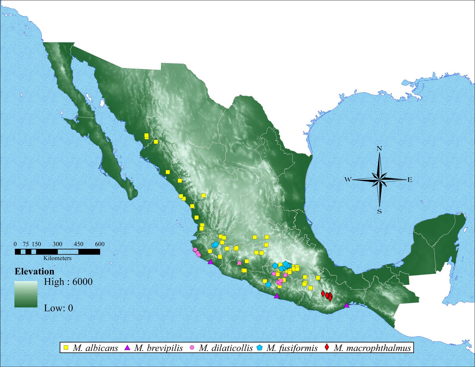
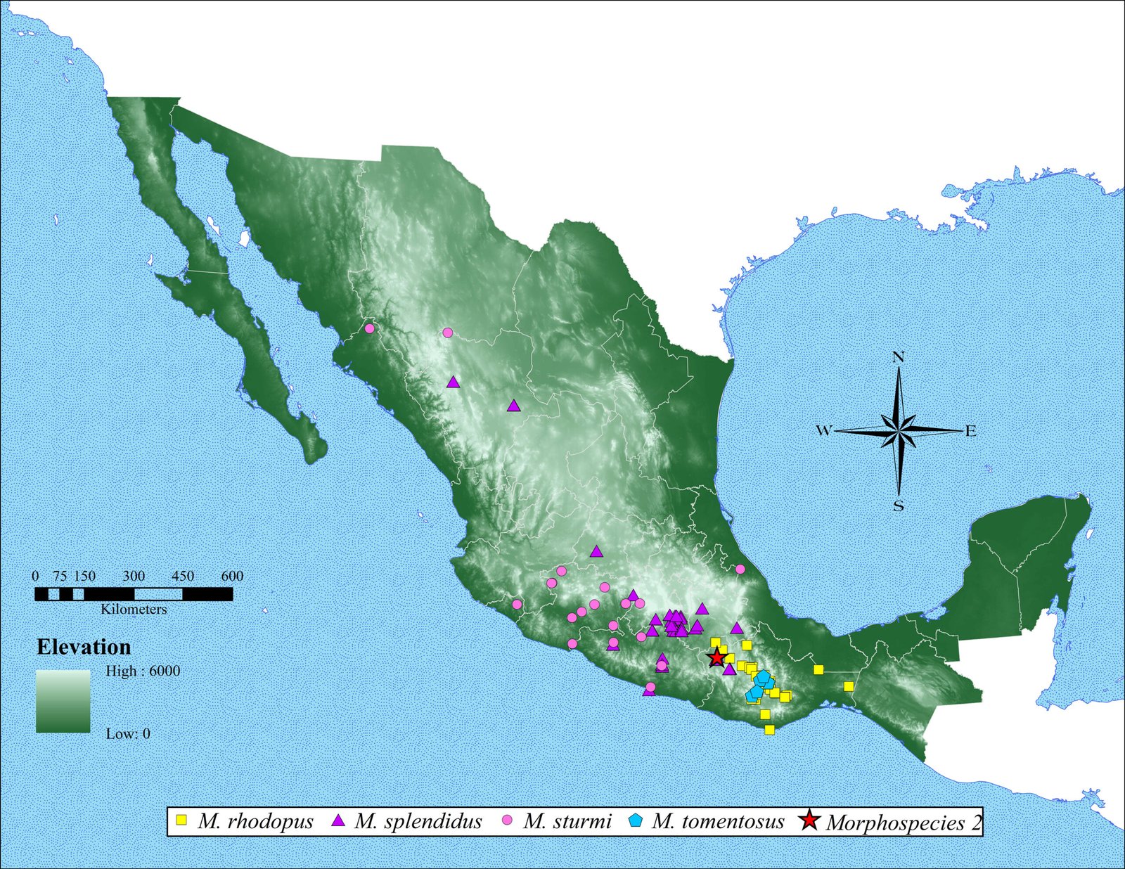
Geographic distribution. The maps (Figs. 7, 8) indicate that the species of Megalostylus are mostly distributed along the Pacific coast, with the greatest richness in the central and southern parts of the country. Megalostylus albicans shows the largest distribution,ranging from Oaxaca to Sinaloa. Six species are distributed in the central states of the country (Guanajuato, Guerrero, Michoacán, Morelos, and Puebla): M. albicans, M. brevipilis, M. dilaticollis, M. fusiformis, M. splendidus, and M. sturmi. The species M. rhodopus, M. macrophthalmus, and M. tomentosus are restricted to Oaxaca, and M. rhodopus reaches the southernmost distribution extending to the Isthmus of Tehuantepec.
Discussion
The sister group relationship between Megalostylodes and Megalostylus is well supported by 12 exclusive synapomorphies, and the monophyly of Megalostylus is supported by a combination of 4 exclusive synapomorphies of the protibiae, elytra, and female and male genitalia. Champion (1911) distinguished Megalostylus based on the presence of a prominence opposite to mucro (or toothed tibiae at the external apical angle), and Lanteri and del Río (2017) recovered this character state (car 69[1]) as an apomorphy of Megalostylus.
Within Megalostylus most of the relationships are not well supported nevertheless, it is clear the position of M. rhodopus (including morphospecies 1 and 3) as sister species of the remaining, and it was recovered a well-supported group including M. dilaticollis (= morphospecies 5), M. albicans, M. brevipilis, M. fusiformis, M. splendidus, and M. sturmi. Megalostylus macrophthalmus and M. tomentosus (= morphospecies 4) would be basal regarding this clade. Morphospecies2 is considered a probable new species, however, this status needs further studies.
Figure 5. Diagrammatic illustrations with arrows and numbers indicating character codification of female and male genitalia in Megalostylus and outgroup species. A) Pantomorus albosignatus, spermatheca; B) M. albicans, spermatheca; C) M. splendidus, sternite VIII; D) Megalostylodes hirsutus, sternite VIII; E) M. rhodopus, aedeagus; F) M. sturmi, aedeagus. Scale bars = 0.5 mm.
The species of Megalostylus are very variable in scale color, size and pronotum shape, and due to that intraspecific variation, some nominal species have been synonymized: M. farinosus Chevrolat, 1878 [junior synonym of M. albicans (Lacordaire, 1876)], M. expansus Pascoe, 1881 [junior synonym of M. albicans (Lacordaire, 1876)] and M. villosus Chevrolat, 1878 [junior synonym of M. sturmi Boheman, 1840]. Our analysis explored the relationships among intraspecific varieties of the genus Megalostylus, and the results support the previously established synonymies. In the case of M. albicans with its varieties (M. albicans var. expansus and M. albicans var. farinosus) there is no reason to consider them as different species. Characters with the greatest contribution to the species relationships are those referring mainly to the vestiture of antennae, legs, elytra, shape, and characteristics of the pronotum, scutellum, and apex of aedeagus.
Figure 6. Most parsimonious cladogram of Megalostylus plus 3 outgroups under equal weights, showing character fast optimization. Black circles indicate synapomorphies, whereas white circles indicate non-exclusive synapomorphies. Numbers on and below each circle correspond to character and state codes, respectively. Bootstrap values are indicated below the branches. Figure 7. Occurrence map of 5 Megalostylus species, ordered alphabetically. Megalostylusalbicans (yellow square); M. brevipilis (purple triangle); M. dilaticollis (pink circle); M. fusiformis (blue pentagon) and M. macrophthalmus (red diamond). Map by A. Lizama-Hernández. Figure 8. Occurrence map of remaining 4 Megalostylus species, ordered alphabetically plus a new Megalostylus species (indicated here as morphospecies 2). Megalostylus rhodopus (yellow square); M. splendidus (purple triangle); M. sturmi (pink circle); M. tomentosus (blue pentagon) and morphospecies 2 sp. nov. (red star). Map by A. Lizama-Hernández.
Acknowledgments
We thank all curators, institutions, collection managers, technicians, and collectors that provided specimens. We also thank Miguel Menéndez-Acuña, Elizabeth Arellano-Arenas, and anonymous reviewers for their helpful suggestions to improve the manuscript. The authors would like to express their sincerest gratitude to Santiago Zaragoza Caballero and María Cristina Mayorga Martínez for their invaluable assistance in providing material for examination.
References
Champion, G. C. (1911). Insecta. Coleoptera. Vol. IV, Parte 3. Rhynchophora. Curculionidae. Attelabinae, Pterocolinae, Allocoryninae, Apioninae, Thecesterninae, Otiorhynchinae. In D. Sharp, & G. Champion (Comps.), Biologia Centrali-Americana (pp. 241–246). London: R.H. Porter.
del Río, M. G. (2009). Estudio taxonómico y cladístico de los géneros de la tribu Naupactini (Coleoptera: Curculionidae) distribuidos en la subregión Páramo-Puneña o Zona de Transición Sudamericana (Ph.D. Thesis). Universidad Nacional de la Plata, La Plata, Argentina.
ESRI (2015). ArcGIS Desktop: Versión 10.4.1 Redlands, CA: Environmental Systems Research Institute.
Goloboff, P. A., & Catalano, S. A. (2016). TNT version 1.5, including a full implementation of phylogenetic morphometrics. Cladistics, 32, 221–238. https://dx.doi.org/10.1111/cla.12160
Lanteri, A. A., & del Río, M. G. (2017). Phylogeny of the tribe Naupactini (Coleoptera: Curculionidae) based on morphological characters. Systematic Entomology, 42, 429–447. https://doi.org/10.1111/syen.12223
Maddison, W. P., & Maddison, D. R. (2021). Mesquite: a modular system for evolutionary analysis. Versión 3.70. http://www.mesquiteproject.org
Muñiz-Vélez, R., Burgos-Dueñas, A., Burgos-Dueñas, O., López-Martínez, V., & Burgos-Solorio, A. (2015). Nuevas aportaciones a los Curculionoidea del estado de Morelos, Folia Entomológica Mexicana, 1, 25–49.
Ordóñez-Reséndiz, M. M., Muñíz-Vélez R., & Gama-Rojas, F. (2008). Curculiónidos (Coleópteros). In S. Oceguera, & J. Llorente-Bousquets (Coords.), Catálogo taxonómico de especies de México, en Capital natural de México, vol. L. Conocimiento actual de la biodiversidad. CD1. Mexico City. Conabio.
Rosas, M. V., Morrone, J. J., del Río, M. G., & Lanteri, A. A. (2011). Phylogenetic analysis of the Pantomorus-Naupactus complex (Coleoptera: Curculionidae: Entiminae) from North and Central America. Zootaxa, 2780, 1–19. https://doi.org/10.11646/zootaxa.2780.1.1
Schoenherr, C. J. (Ed). (1840). Genera et species curculionidum, cum synonymia hujus familiae; species novae aut hactenus minus cognitae. Paris: Roret.
Francisco J. García-De León a, Gorgonio Ruiz-Campos b, *, Jesús Roberto Oyervides-Figueroa c, Gonzalo De León-Girón b, Carlos Alberto Flores-López b, Dante Magdaleno-Moncayo d, Alicia Abadía-Cardoso e
a Centro de Investigaciones Biológicas del Noroeste, S.C., Laboratorio de Genética para la Conservación, Av. Instituto Politécnico Nacional 195, Playa Palo de Santa Rita Sur, 23096 La Paz, Baja California Sur, Mexico
b Universidad Autónoma de Baja California, Facultad de Ciencias, Carretera Ensenada-Tijuana Km. 103 s/n, 22860 Ensenada, Baja California, Mexico
c Centro de Investigación Científica y de Educación Superior de Ensenada, Departamento de Acuicultura, Carretera Tijuana -Ensenada 3918, Zona Playitas, 22860 Ensenada, B.C., Mexico
d Universidad Autónoma de Baja California, Facultad de Ingeniería, Arquitectura y Diseño, Carretera Ensenada-Tijuana Km. 103 s/n, 22860 Ensenada, Baja California, Mexico
e Universidad Autónoma de Baja California, Facultad de Ciencias Marinas, Carretera Ensenada-Tijuana Km. 103 s/n, 22860 Ensenada, Baja California, Mexico
*Corresponding author: gruiz@uabc.edu.mx (G. Ruiz-Campos)
Received: 20 August 2024; accepted: 20 February 2025
Abstract
We assembled and annotated the mitochondrial genome of golden eagles from the northwest of Baja California, Mexico, using reference and de novo strategies to analyze the synteny of mitochondrial genes, the phylogenetic relationships, and genetic variation of mitochondrial DNA. The length of the Golden Eagle mitogenome was 17,472 bp (base pairs) with a base composition of A (29.8%), C (32.5%), G (14.0%), and T (23.6%). The mitogenome contains 13 genes coding for the protein complexes coxI II-III, Cytb, cATP 6 and 8, and Nicotinamide Adenine Dinucleotide (NADH 1-6); this arrangement is consistent with the general model of the mitogenome reported in other congeneric members. Mitogenomes of individuals from northwestern Baja California are unique and they differ from the mitogenome of southern California golden eagles in 3 traits: 1) molecule size is 140 bp larger than that previously reported, 2) the addition in the annotation of a region called pseudo control (ψRC), and 3) the annotation in 2 fractions of the coding region for the protein NADH dehydrogenase subunit 3 (ND3). The genetic diversity and phylogenetic analyses of the individual genes and mitogenome support a close genetic relatedness between the golden eagles from northwestern Baja California and southern California region.
Keywords: Mediterranean region; Mitochondrial lineages; Mitochondrial genome; Next generation sequencing; Non-model species
Mitogenoma de águila real (Aquila chrysaetos) en el noroeste de Baja California, México: relaciones filogenéticas y variación genética
Resumen
Ensamblamos y anotamos el genoma mitocondrial del águila real del noroeste de Baja California, México, utilizando estrategias de referencia y de novo para analizar la sintenia de genes mitocondriales, las relaciones filogenéticas y la variación genética del DNA mitocondrial. La longitud del mitogenoma fue 17,472 pb (pares de bases) con una composición de bases de A (29.8%), C (32.5%), G (14.0%) y T (23.6%). El mitogenoma contiene 13 genes codificantes de los complejos proteínicos coxI II-III, Cytb, cATP 6 y 8, y nicotinamida adenina dinucleótido (NADH 1-6); esto fue consistente con el modelo general del mitogenoma reportado en otros congéneres. Los mitogenomas de individuos del noroeste de Baja California son únicos y se diferencian del mitogenoma de individuos del sur de California en 3 rasgos: 1) el tamaño de molécula es 140 pb más grande que el reportado, 2) adición de la región llamada pseudocontrol (ψRC) y 3) anotación en 2 fracciones de la región codificante de la proteína NADH deshidrogenasa subunidad 3 (ND3). La diversidad genética y los análisis filogenéticos de los genes individuales y el mitogenoma respaldan una estrecha relación genética entre las águilas reales del noroeste de Baja California y la región del sur de California.
Palabras clave: Región mediterránea; Linajes mitocondriales; Genoma mitocondrial; Secuenciación de próxima generación; Especies no modelo
Introduction
The Golden Eagle, Aquila chrysaetos, is an accipitrid of boreal distribution that inhabits a variety of open and semi-open biotopes from sea level to 3,630 m in altitude in biomes as tundra, chaparral, temperate grassland, temperate deciduous forest, and coniferous forest (De León-Girón et al., 2016; Flesch et al., 2020; Kochert et al., 2002; Watson et al., 2011). This emblematic species is known to occur in Mexico in the arid and semiarid environments of the northern and central regions, including some locations as south as Oaxaca (Bolger et al., 2014; De León-Girón et al., 2016; Howell & Webb, 1995; Rodríguez-Estrella, 2002; Rodríguez-Estrella et al., 1991, 2020). Although the demography of the Golden Eagle has been determined with different genetic methods that confirm the structuring of its populations (Craig et al., 2016; Doyle et al., 2016), little is known about the genetic identity of populations of this eagle in its distribution range. Northwestern Baja California is considered the greatest nesting and conservation potential region for the Golden Eagle in Mexico (De León-Girón et al., 2016; Rodríguez-Estrella, 2002; Rodríguez-Estrella et al., 1991; Tracey et al., 2017), with vast areas of habitats still pristine for the population conservation of this species shared with the United States of America (Craig et al., 2016; De León-Girón et al., 2016, 2024; Doyle et al., 2014; Katzner et al., 2023).
Studies based on mitochondrial DNA (mtDNA) allow determining the current state of conservation of species, as well as the identification of significant evolutionary and management units with their demographic aspects (Moritz, 1994). With the advent of next-generation sequencing (NGS) technologies (especially on complete mitochondrial genomes), new studies with non-model species became more common. As was the case for various species of the family Accipitridae, including the Golden Eagle. Doyle et al. (2014) were the first to describe the nuclear and mitochondrial genome of the Golden Eagle from the central California region, in the USA.
In this study we focus on the synteny of mitochondrial genes, the phylogenetic relationships, and the mitochondrial genetic diversity among Golden Eagle individuals in northwestern Baja California, Mexico. Given the high migration potential of this species, individuals collected in northwestern Baja California are predicted to be phylogenetically related to the westernmost Golden Eagle population in the USA. Therefore, studies focused on examining the genetic variation at the mitochondrial level will allow better decision-making for management and conservation programs for the species in a binational spectrum. In the same way, our study will be a valuable reference for analyzing other Golden Eagle populations in Mexico and other regions of its distribution range.
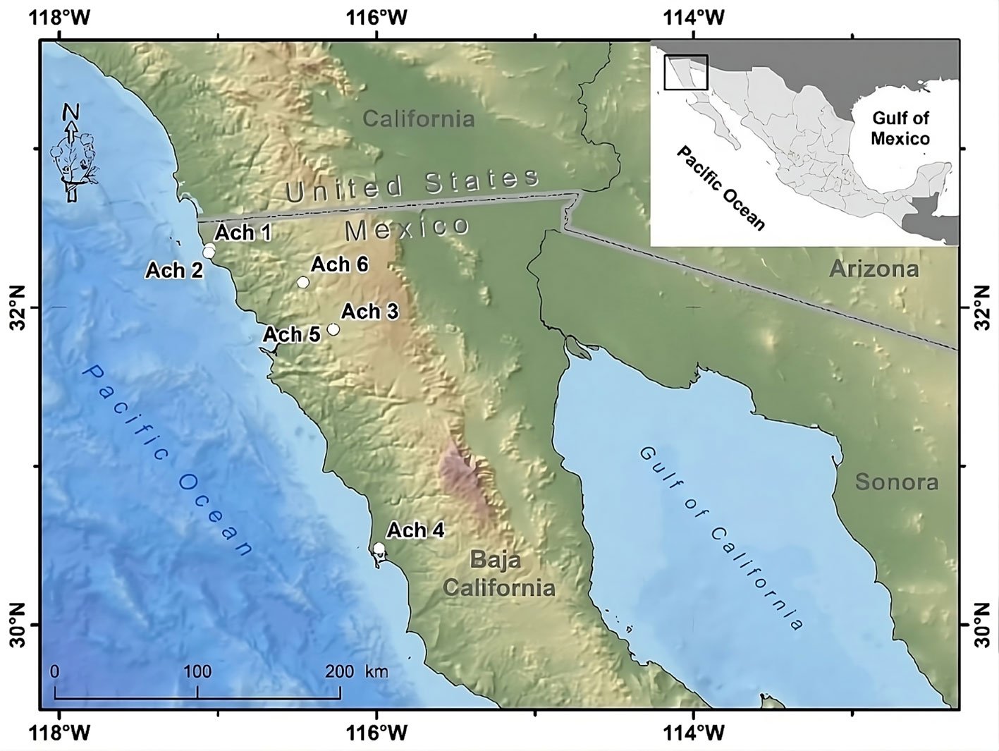
Figure 1. Geographical location of the Golden Eagle voucher specimens examined for mitogenome in the northwestern Baja California, Mexico. Geographic coordinates for each individual can be found in Supplementary material T1. Map by Rafael Hernández Guzmán.
Materials and methods
Tissue samples of 6 Golden Eagle specimens from northwestern Baja California, Mexico were obtained. These specimens were found dead in different agriculture valleys of the Mediterranean region in northwestern Baja California, Mexico, between the municipalities of Rosarito and San Quintín, from 1995 to 2014, and deposited as vouchers in the Bird Collection of the Science Faculty, at the Autonomous University of Baja California (UABC), campus Ensenada (Fig. 1, Supplementary material: T1).
For the DNA extraction, tissue samples of the pads of the feet of 5 Golden Eagle specimens referred to here as Ach 1 to Ach 5 were obtained. DNA using the nucleic acid purification method by differential saline precipitation (Aljanabi & Martinez, 1997) was extracted. Both feathers and blood for the Ach 6 sample (Supplementary material: T1) were used and extracted DNA with the Qiagen Blood & Tissue kit. The quality and quantity of the extracted DNA in both cases was evaluated using Nanodrop, Qubit and agarose gel electrophoresis.
Extracted DNA (from 77 to 210 ng/µL per sample quantified in Nanodrop for Ach1-Ach5 individuals and 0.581 ng/µL for Ach6 quantified in Qubit) was purified with SpeedBeads magnetic beads (Thermo-Scientific, Waltham, MA, USA) at a 1.2:1 beads:DNA ratio and resuspended in 50 µl of TLE1X buffer. Libraries for shotgun sequencing were prepared, for which purified DNA from each individual was fragmented by sonication in a Bioruptor® (Diagenode, Liege, Belgium) using 2 rounds, each consisting of 5 cycles of 30 sec of sonication and 30 sec without sonication at the highest setting. DNA fragments were then prepared using the Kapa Biosystems® Hyper Prep Kit (KR0961–v4.15, Roche, Basel, Switzerland), with which end repair and A-tailing were performed, adapters were ligated, and PCR was performed with indexed primers (Glenn et al., 2020) for 14 cycles. Following amplification, fragment size selection was performed by double-dip with SpeedBeads magnetic beads (Thermo-Scientific, Waltham, MA, USA) that allow to preserve fragments between ~250 and ~700 base pairs (bp) for each of the samples, which are the appropriate insert size for the Illumina platform. Sequencing was performed paired end on 2 different platforms. We sequenced the Ach1-Ach5 samples on the Illumina MiSeq V.3 at the Georgia Genomics and Bioinformatics Core (GGBC) to generate 300-bp paired-end fragments, and we sequenced Ach6 on an Illumina HiSeq 4000 at the Oklahoma Medical Research Foundation Clinical Genomics Center to generate 150-bp paired-end fragments.
Bioinformatic analysis. The quality of the raw sequences was evaluated using the FastQC program (Andrews, 2010). Subsequently, the sequences using a standard treatment were filtered using the Trimmomatic software (Bolger et al., 2014) with 4 steps. In the first step, the sequencing adapters and over-represented sequences were removed by means of the ILLUMINACLIP function. The second step discarded sequences with a quality value below 30 QS with the AVGQUAL function. The third step removed fragments below 25 QS with the SLIDINGWINDOW function. The fourth step did an even stricter cleanup using MAXINFO. This step conserved sequences of at least 100 base pairs and was configured to preferentially conserve longer sequences with a value of 0.3. For the Ach 5 specimen, an extended and modified version of the standard treatment was used due to the low quality of sequences. This involved applying the SLIDINGWINDOW function, which modifies the quality value.
Assembly and annotation. Two strategies were followed to assemble the mitochondrial genomes: the reference based and the de novo strategy (Machado et al., 2015, 2018). Mapping against a reference mtDNA genome was performed using the Bowtie2 program version 2.3.4.2 with clean reads (Langmead & Salzberg, 2012). The reference mitochondrial genome was from the same species A. chrysaetos, with the GenBank accession number of KF905228.1. De novo assembly only for samples Ach 2 to Ach 6 was performed using the A5-miseq pipeline (Coil et al., 2015). Due to the large number of reads after the filter (Supplementary material: T2) sample Ach 1 was analyzed with the Velvet software version 1.1 (Zerbino & Birney, 2008). The mitogenome was annotated from the scaffolds obtained from the de novo assemblies. We determined scaffolds longer than 4 Kpb by applying a search with the BLAST tool (Basic Local Alignment Search Tool) of the NCBI (National Center for Biotechnology Information) website. The scaffolds were aligned to achieve greater coverage considering the length of the reference genome used previously. Afterwards, RNAweasel (http://megasun.bch.umontreal.ca/RNAweasel/) was implemented to the identification of tRNA’s (transfer RNA), rRNA’s (ribosomal RNA) and introns and, in turn, MFannot (http://megasun.bch.umontreal.ca/RNAweasel/) for the identification of proteins and open reading frames (Sieber et al., 2018).
In addition to the previous annotation, MITOS web server (Bernt et al., 2013) was used to assist in the annotation of de novo mitochondrial genomes, allowing gene names, tRNA and rRNA secondary structures, and codon usage to be obtained. Finally, a manual curation of the annotations was used to review the 6 existing reading frames with the UGENE software (Okonechnikov et al., 2012). The control region was identified based on 99% similarity with an A. chrysaetos partial control region sequence (EF459579.1). Genome Vx software (Conant and Wolfe, 2008) was used to map the Golden Eagle’s mitogenome, using individual Ach 6 to achieve this analysis.
In the annotation of the de novo assembly, the ND3 protein appeared divided into 2 fractions (see Results), a trait that was not reported by Doyle et al. (2014). Therefore, an experimental verification was required through PCR amplification and its subsequent Sanger sequencing. We designed primers from de novo assembly using the NCBI Primer-BLAST program: ND3Ach-1 (5’GCCTGATACTGGCACTTCGT3’ and 5’CCCTATCAATCTGACCCACCG3’) which generates a 716 bp fragment and ND3Ach-2 (5’CTTCTTCGTCGCTACAGGCT3’ and 5’CCTTCCACCGAACCCACTTAA3’) which generates a 774 bp fragment. Eight Golden Eagle samples from the Ornithological Collection of the Faculty of Sciences of the Autonomous University of Baja California were used for PCR amplification. These samples correspond to the 6 individuals used for sequencing and 2 extra samples that are not part of the mitogenome assembly study. The conditions of the PCR reaction were as follows: 6 min at 94°C, 35 cycles of denaturation, annealing, and extension at 94°C for 30 sec, 51°C for 30 sec and at 72°C for 1.5 min, respectively. A final elongation stage at 70°C for 7 min, and a final conservation stage at 15°C. We sent the amplified fragments for sequencing to the SeqXcel.inc Company in San Diego, California, and analyzed with the ABI PRISM® 3130xl Genetic Analyzer DNA kit.
Synteny and search for polymorphisms. A posteriori synteny analysis was performed between the Golden Eagle mitogenome reported by Doyle et al. (2014) and the newly assembled mitochondrial genome of this study. This analysis was carried out with the MAUVE software (Darling et al., 2004). The same reference mitogenome was used to call SNP’s and INDEL’s for the 6 genomes assembled in this work using the SAMtools program (Li, 2011). Filtering the call quality of the variants involved discarding those with a value less than 20 Qs and keeping those with at least 5X depth (Li, 2011). Each variant was manually evaluated, retaining SNPs and INDELs where at least half of the aligned reads showed the change and verified its existence in at least one other individual (Fridjonsson et al., 2011).
Phylogenetic relationships. Phylogenetic relationships were inferred using the individual gene dataset and the mitogenome. The individual gene fragments analyzed consisted of the ND2, ND3, coxI and Cytb recovered from Aquila chrysaetos individuals from GenBank (Supplementary material: T3) and those produced in this study. The mitogenome analysis for phylogenetic relationships consisted of 10 complete mitogenomes: 6 obtained in this study, 2 reference samples of Aquila chrysaetos (LR822062 from the United Kingdom and NC_024087.1 from California, USA), 1 reference sample classified as Aquila heliaca (NC_035806.1), but has been reported to actually consist of a A. chrsyasetos individual (Sangster & Lukesenburg, 2021) and 1 outgroup (Aquila nipalensis, GenBank accession number NC_045042.1). Both datasets were aligned using the MAFFT 7 algorithm (Katoh & Standley, 2013). Removing the non-conserved regions between the sequences of the multiple alignments was done using the online program Gblocks with the default parameters (Castresana, 2000). The nucleotide substitution model and the mutation rate were determined using JModelTest (Posada, 2008), considering the Bayesian information criterion (BIC).
Two phylogenetic reconstruction methods were used: Maximum Likelihood (ML) and Bayesian analysis. In IQ-TREE (Nguyen et al., 2015) the ML method (Felsenstein, 1981) was run with the DNA substitution model selected by ModelFinder (Kalyaanamoorthy et al., 2017) and 1,000 bootstrap pseudo replicates were performed (Hoang et al., 2017). Bayesian inference was used with MrBayes program (Ronquist et al., 2012); for this, 4 Markov Monte Carlo chains (MCMC) were implemented with a total of 10 million generations, and a sampling every 1,000 generations. To construct the consensus phylogenetic tree, a 25% of burn-in was applied. The support of the nodes was evaluated via the posterior probability values. The results of both approaches were visualized with FigTree 1.4 (Rambaut, 2009). For the mitogenome phylogenetic tree, the dataset on genes that were annotated across the entire mitogenome were partitioned (Supplementary material: T4). To determine the most appropriate DNA substitution model for each gene, the Akaike Information Criterion test implemented in jModelTest2 (Darriba et al., 2012; Guindon & Gascuel, 2003) was used (see selected models for each gene in Supplementary material: T4). The partitioned mitogenome dataset was used to estimate a Bayesian phylogenetic tree in MrBayes (Ronquist et al., 2012). The Bayesian analysis was carried out by running 4 MCMC chains for 5 million generations and saving the trees every 1,000 generations. The consensus phylogenetic tree was constructed using a 10% burn-in.
Genetic diversity. Individual DNA segments from the coxI, Cytb, ND2, and -ND3 genes were used to estimate the genetic diversity parameters for the A. chrysaetos species complex since these were the genes that had a relative amount of A. chrysaetos DNA sequences available in GenBank. Using DNA sequences from the Baja California individuals produced in this study and reference sequences from the species complex (Supplementary material: T3) the following indices were estimated with DnaSP 6 (Rozas et al., 2017): the number of segregating sites (S), number of haplotypes (Nh), haplotype diversity (Hd), and nucleotide diversity (π). Genetic diversity indices were calculated among all sequences included in the respective datasets and within specific groups of sequences according to phylogenetic clades or geographic origin of samples. In addition, the genetic distance (uncorrected p-distance) between and within the phylogenetic clades observed within the mitochondrial genetic lineages in PAUP software was estimated (Swofford, 1993). The clade OTU1 included sequences from a diverse geographical background, including all the DNA sequences of the Baja California golden eagles. In contrast, the A. chrysaetos DNA sequences grouped in the other closely related clade were classified as OTU2. Additionally, the DNA sequence of an individual of A. chrysaetos from California (Southern Sierra Nevada) was analyzed separately to compare its genetic distance with those from Baja California, given the geographical proximity between both populations.
Results
Raw sequencing reads ranged from 3,324,579 (individual Ach 1) to 539,825 (individual Ach 4). The number of total sequences after the filter ranged between 3,251,746 (Ach 1) and 526,875 (Ach4) (Supplementary material: T2A).
Assembly and annotation. There were large differences in assembly between individuals; for example, the average depth in the reference mapping for individual Ach 1 is 30.5X, while for Ach 6 is 168.3X, even though Ach 6 had fewer total reads than Ach 1. Assemblies for individuals Ach 1-5 showed fewer aligned sequences (Supplementary material: T2A). For de novo assembly, the average depth for individual Ach 6 is 8.0X. The longest scaffold generated (17,472 bp) allowed us to assemble the entire mitogenome of the Ach 6 individual, eliminating the need to align multiple scaffolds to recover the full length (Supplementary material: T2B). The data yield was inferior when doing de novo assembly for Ach 1-5 individuals, and none of these individuals allowed the recovery of the complete mitochondrial genome (Supplementary material: T3B).
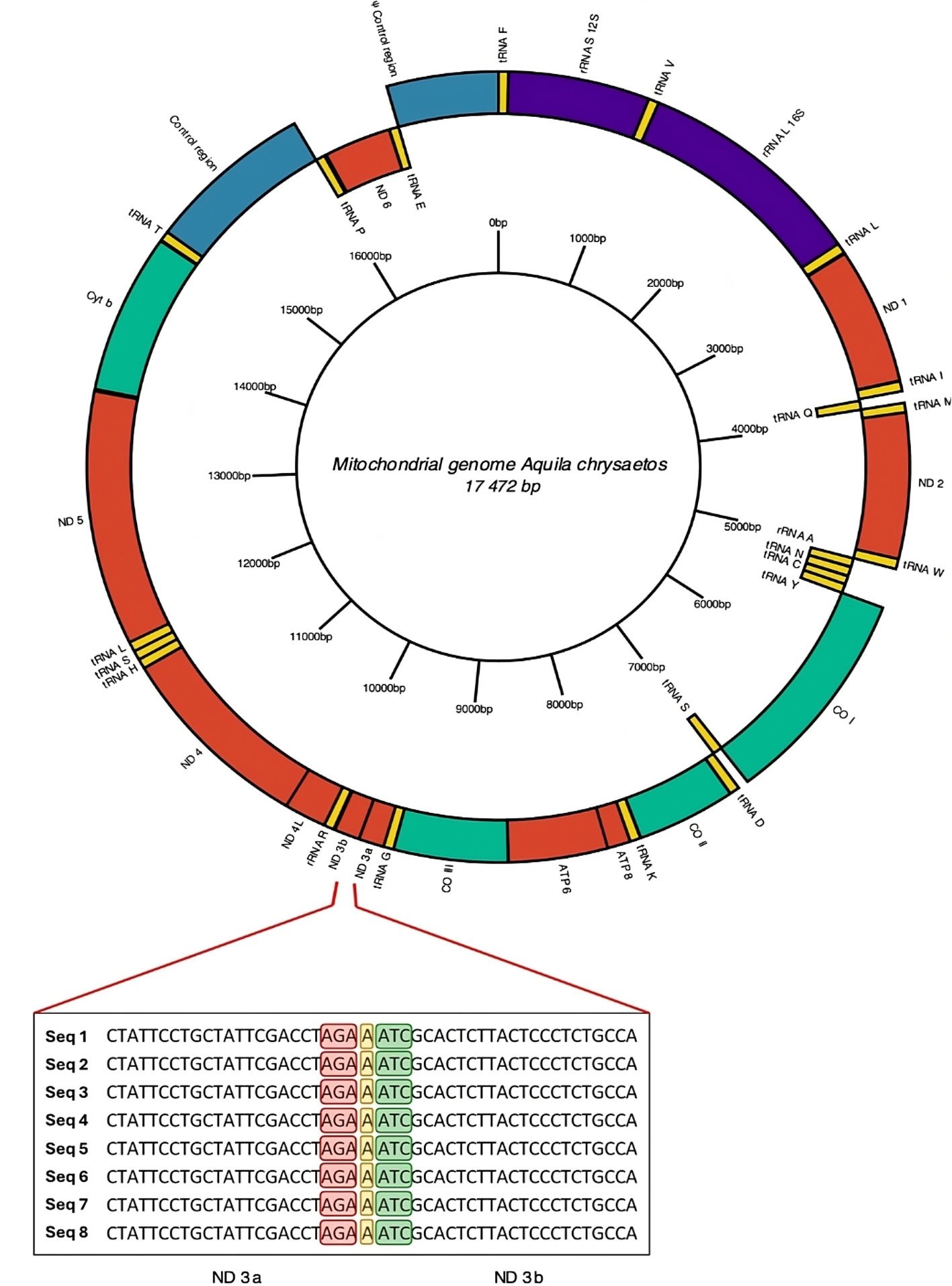
Figure 2. Mitogenome annotated by de novo assembly for Golden Eagle (Ach6) from Baja California, Mexico. In the central part of the diagram in a ring form is shown a scale of the length of mitochondrial genome clockwise. Enlarged view of the section showing the division into 2 fractions of the mitochondrial gene for NADH dehydrogenase subunit 3 (ND3). The stop codon of the ND3a fraction is highlighted in red, the insertion of nucleotide A in yellow, and the start codon of the ND3b fraction in green. The ND3 gene is composed entirely of 352 bp; the ND3a fraction is 207 bp long, while the ND3b fraction is 144 bp long.
Based on the above results, we annotated and curated the mitochondrial genome using only the complete mitogenome obtained by de novo assembly of the Ach 6 individual. All 3 annotation tools identified tRNAs, and none of the tools identified introns within the sequence. The MITOS program (Fig. 2, Supplementary material: T4) was the only software that identified all the genetic elements, such as the 22 tRNAs, 2 rRNAs, and the 13 protein-coding genes that make up the mitogenome. This last annotation was the most complete, so the curation was made from it. We found a region with 7 nucleotide bases that is composed of an AGA stop codon of the ND3 protein, followed by an adenine (A) and finally an ATC start codon that codes for isoleucine. This region divides the ND3 fragment into the 2 regions proposed here (ND3a and ND3b, Fig. 2).
Synteny and search for polymorphisms. The linear order of the mitogenome of Ach 6 coincides with the reference genome (Accession number MT319112.1, Supplementary material: T5). We consider the SNPs and INDELs identified in the Ach 6 reliable, given that the average coverage is 168.3X, and their call quality was high (Supplementary material: T2A). Most SNPs and INDELs are found within genes that code for some protein, transfer RNA and ribosomal genes. The coxI gene presented the greatest number of SNPs with respect to the reference genome in the 6 individuals, while the Cytb and tRNA F genes presented the greatest length changes in the INDELs. In addition, in the ND3 gene, there is a consistent change in the sequences of the 6 individuals with respect to the reference genome (Table 1).
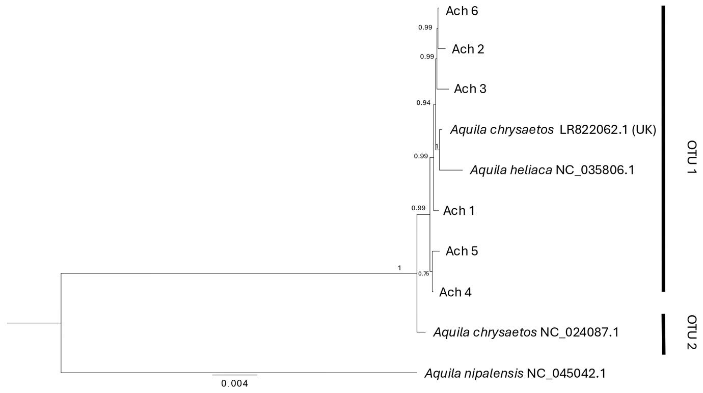
Figure 3. Bayesian phylogenetic tree based on the mitogenome for Golden Eagle voucher specimens from northwestern Baja California, Mexico. Posterior probabilities are shown above internal nodes. GenBank accession numbers are positioned next to reference sequences. Aquila nipalensis was used as an outgroup for rooting the tree. Two Operational Taxonomic Units are identified (OTU 1, 2).
Phylogenetic relationships. With the use of the mitogenome we constructed a phylogenetic tree that identified 2 clades with strong support (1): OTU1 that includes all the individuals analyzed in this study, plus 2 GenBank sequences (Aquila chryseatos, LR82062.1 from the United Kingdom and A. heliatica, NC_035806.1), and OTU2 that corresponds to a GenBank sequence of a specimen collected in California (Fig. 3). For their part, the phylogenetic trees obtained with the fragments of individual genes (ND2, ND3, Cytb and coxI) did not resolve the divergence between individuals from Baja California and California obtained with the mitogenome, but all except the ND3 gene showed a divergence (OTUs 1 and 2), mainly with respect to eagles from the European continent (when information on the collection location is reported, Supplementary material: F1).
Genetic diversity. We observed low genetic diversity, for instance, ND3, ND2, and coxI each had a single segregating site (Table 2), resulting in low nucleotide diversity values (0.0005, 0.0008, and 0.0002, respectively). In contrast, Cytb was the most polymorphic, with a total of 10 segregating sites and a nucleotide diversity an order of magnitude larger (0.00297) (Table 2). The genetic diversity found within OTU1 was higher than that found in OTU2 (Table 2), although OTU1 was not a geographically homogeneous clade among the trees of the different mitochondrial genes, for example in the case of ND2 it was made up of North American eagles, including the individuals of this study, but coxI apart from the previous ones was constituted with eagles from Sweden, Norway and Japan (Table 2).
Discussion
Despite using 2 sequencing platforms for the mitogenome of Golden Eagle from northwestern Baja California, Mexico, we successfully assembled the mitochondrial genome of all 6 individuals by the reference method. This included some individuals (Ach 1-5) with non-consensus regions. Bolger et al. (2014) recommend a pre-processing step of the readings before any analysis, be it assembly by reference or de novo, and mention that if the library and identification adapters are not removed, they can be incorporated in the final assembly. In our case, the pre-processing of the sequences positively influenced the performance of both assemblies and the SNP’s call since the quality of the sequence of the 6 individuals was considerably improved after pre-processing in all aspects of quality reporting.
Table 1
Location of SNP’s and INDEL’s in mitogenomes. Call of SNP’s and INDEL’s for each the Ach 1-6 specimens versus the reference genome of Golden Eagle from the southern Sierra Nevada in California, USA (GenBank accession: KF905228). Pos: Mitogenome position; Ref: nucleotide present in reference sequence. ψCR: Mitochondrial pseudogene control region.
Pos.
Ref.
Ach1
Ach2
Ach3
Ach4
Ach5
Ach6
Gen
SNP’s
1,505
G
A
A
A
D-loop
1,515
T
C
3,130
G
A
A
A
3,566
A
G
ND6
3,695
T
A
A
A
3,696
T
A
A
A
5,557
G
A
A
A
A
A
LSU rRNA
6,646
G
A
A
A
ND1
7,141
A
G
8,269
C
T
A
T
ND2
8,593
A
G
G
A
G
8,723
G
A
A
A
A
tRNA-Trp
10,925
C
T
T
T
T
T
10,963
T
C
10,970
C
T
T
T
T
T
10,975
T
C
coxII
11,003
A
G
G
11,011
C
T
11,205
A
G
11,213
C
T
11,237
C
T
11,282
G
A
11,284
G
T
11,285
A
C
11,351
T
C
11,354
A
G
11,378
C
T
T
11,432
C
T
T
T
T
T
11,489
A
C
C
C
C
C
C
11,493
T
T
tRNA-Lys
11,496
G
A
11,505
T
G
17,278
G
A
A
ND5
INDEL’s
Table 1. Continued
Pos.
Ref.
Ach1
Ach2
Ach3
Ach4
Ach5
Ach6
Gen
3
CTAA
CTAA CTTC CAAA CTAA
Cyt b
3,550
T
TGTG AACA A
ψCR
3,701
CAAA
CCCA CCAA TA
CCAA CAAT AT
tRNA-Phe
13,378
T
TC
TC
TC
TC
TC
TC
ND3
Table 2
Genetic diversity and haplotype composition from gene segments. Tax Set: Group of sequences included in taxonomic set; N: number of sequences; bp: base pairs of DNA sequence included in alignment; S: number of segregating sites; Nh: number of haplotypes; Hd: haplotype diversity; Nd: nucleotide diversity; North America: sequences from either Canada or USA. All sequences from ND3 formed a single clade, and thus were analyzed as a single group. OTUs 1 and 2 in each individual gene refer to the clades detected in each phylogenetic analysis, see Supplementary material F1.
Mitochondrial sequence
Tax Set
N
bp
S
Nh
Hd
Nd
ND3
All
11
352
1
2
0.182
0.00053
ND2
OTU1
8
1,039
0
1
0
0
OTU2
4
1,039
0
1
0
0
North America
2
1,039
0
1
0
0
Europe
3
1,039
0
1
0
0
All
12
1,039
1
2
0.485
0.00087
coxI
OTU1
13
1,551
1
2
0.154
0.00025
OTU2
2
1,551
0
1
0
0
North America
4
1,551
0
1
0
0
Europe
4
1,551
1
2
0.5
0.00082
All
15
1,551
1
2
0.133
0.00022
Cytb
OTU1
13
1,143
1
2
0.154
0.00016
OTU2
3
1,143
1
2
0.667
0.00069
North America
4
1,143
1
2
0.5
0.00052
Europe
5
1,143
9
3
0.02688
0.00541
All
16
1,143
10
4
0.442
0.00297
The most reliable mitogenome assembly was that of Ach 6 individual due to its higher alignment rate, its greater depth, and its 100% coverage of the reference genome. This ensemble can be considered true and not an artifact due to the procedures used, such as sampling every 500 generations and a burn-in value of 600,000 generations (Lerner & Mindell, 2005). In addition, we analyzed the data with Bowtie2, which implements an alignment strategy based on the FM-Index and Burrows-Wheeler. These programs have been shown to work well for applications such as INDEL discovery (Lindner & Friedel, 2012) and for aligning long sections of the reference genome (Thankaswamy-Kosalai et al., 2017). Hunt et al. (2014) pointed out that the best result of assembling a genome de novo is when it is contained in a single scaffold for the entire mitochondrial DNA molecule or for each chromosome in the case of the nuclear genome. The Golden Eagle mitochondrial genome assembly of individual Ach 6 was the best because it was found within a single scaffold (17,472 bp) and its depth was at least 8.0X (Supplementary material: T2B; Baker, 2012).
The extension and position of the genes in the mitogenome of the Golden Eagle described in this study (Fig. 2, Supplementary material: T4) showed differences compared to those reported by Doyle et al. (2014) from an individual sampled in central California. For example, the size of the mitogenome described here is larger (17,472 bp) than the one reported by Doyle et al. (2014) (17,332 bp), with a difference of 140 bp. When experimentally analyzing the size of the ND3 gene amplified fragments, the size was between 700 and 800 bp, that is, the theoretically expected size. Another difference consisted in the fraction of the gene encoding the ND3 protein reported here as split into 2 segments (ND3a and ND3b). The distinction of the 2 subunits is, within the reading frame, a region made up of 7 nucleotides between the ATC start codon that starts the protein, and the TAA stop codon that marks the end of the protein. The first 3 of these 7, code for a new AGA stop codon, followed by an adenine (A) nucleotide and 3 nucleotides that code for a new ATC start codon. This causes 2 coding portions to coexist, annotated as ND3, separated by a single nucleotide that changes the reading frame, causing the second portion to appear with its start and stop codons. Mindell et al. (1998) report a nucleotide that is not translated within the ND3 protein sequence. Eberhard and Wright (2016) mentioned that such a trait is observed in the entire order Psittaciformes (parrots, parakeets, and allies).
Specifically, a variety of distinct indels have been found within several of the mitochondrial protein-coding genes in Psittaciformes (Eberhard & Wright, 2016), with variations in terms of their evolutionary origin since some are present in all Psittaciformes and some are more recent in origin and only found within specific taxa. Slack et al. (2003) reported variation in the length of the mitochondrial ND6 gene in other avian taxa. Overall, the biological implications of these variations remain unclear until more studies on the proteins are performed to determine if the protein compositions become altered by these variations. However, the experimental verification carried out in the present study strengthens our annotation as 2 fractions for the ND3 region of the A. chrysaetos mitogenome. Also, we noted the regulatory non-coding region (the pseudo control region, ψCR) to be highly conserved among the A. chrysaetos individuals analyzed, which is a relatively conserved region within the order Accipitriformes (cf. Song et al., 2015) and is also found in the same position between the tRNA -E and tRNA-F, as shown by Liu et al. (2017) for the mitogenome of Accipitergularis, another congeneric species.
Synteny and search for polymorphisms. The assembled Golden Eagle mitogenome did not present changes in gene order with respect to the reference (KF905228.1, a male Golden Eagle from southern Sierra Nevada, California). As expected, neither did it present changes in the order of the genes with respect to other species of the same group of birds (Accipitridae), such as Buteo buteo (Haring et al., 2001), Accipiter virgatus (Song et al., 2015), Aquila fasciata (Jiang et al., 2015) and Accipiter gularis (Liu et al., 2017). In addition, it is consistent with one of the general models of the birds’ mitogenome that is characterized by a duplication of the control region and other adjacent genes, which were subsequently degraded, giving rise to the ψCR (Eberhard & Wright, 2016). SNP’s and INDEL’s observed in the mitogenome of the Ach 6 individual meet the needed quality (probability of not being an error) and sequence depth (Li, 2011), so they can be considered as potential markers that should be tested in future population studies, considering some technical aspects, and thus avoid the call of false positives (The 1000 Genomes Project Consortium, 2015).
Reconstruction of phylogenetic relationships. The phylogenetic tree classified all Golden Eagle individuals into 2 mitogenome clades (OTU1 and OTU2). All individuals from Baja California, an individual from the United Kingdom, and an A. heliaca individual clustered within OTU1 (Fig. 3), while OTU2 was composed of a single Golden Eagle individual from California. The genetic distance between the 2 OTUs was 0.002 nucleotide differences per site (Supplementary material: T6). This pattern is not surprising given the poor sampling of taxa for both the mitogenomes and individual genes of A. chrysaetos. Once additional mitogenomes are available for this species, it will become possible to increase the phylogenetic resolution that could confirm or reject the potential presence of multiple mitochondrial lineages circulating within Golden Eagle populations. Nevertheless, given the broad geographic area included in the mitogenome dataset (i.e., an A. chrysaetos individual from the United Kingdom, as well an A. heliaca individual), and the low genetic diversity observed within these mitochondrial sequences (see below), suggests that at the mitochondrial level, the genetic diversity found within A. chrysaetos populations is low.
The use of genes or fragments of the mitochondrial genome allows for the analysis to include a larger data set in the number of locations and individuals. The topology of 3 of the 4 individual gene trees (ND2, Cytb and coxI) did support the presence of at least 2 mitochondrial clades (Supplementary material: F1). However, these gene trees were not consistent when grouping the North American Golden Eagle individuals on the same OTUs.
Future studies targeting molecular markers with a higher mutational rate (i.e., microsatellites) or genomics approach could potentially uncover the presence of genetic differences that are not well defined at the mitochondrial level but might be biologically important. One such difference is seen in the species’ bivalent behavior and its migration pattern in the west (Mcintyre & Lewis, 2016) and northwest of the USA, and through Canada (Bedrosian et al., 2018). The mitogenomic lineages that potentially infer the difference between the eagles of Baja California and central California could correspond to the area where 2 ecological populations are coexisting (De León-Girón et al., 2016). The first population is migratory, originating in western North America (Oregon), while the second lineage is resident in Baja California. According to Craig et al. (2016), this lineage has 1 of the less frequent haplotypes of the mitochondrial control region and is restricted to California. The ability of the Golden Eagle to adapt to different environments (Judkins & Van Den Bussche, 2018), the large dispersal distances of reproductive or floating between Mexico and the USA (De León-Girón et al., 2016, 2024; Rodríguez-Estrella et al., 2020; Tracey et al., 2017), and its extensive home range of reproductive pairs (D’Addario et al., 2019), would support these hypotheses. Besides, the presence of these groups of individuals (reproductive and non-reproductive) in Baja California would be part of the reproductive behavior of the species (Watson et al., 2011), that is, the process of succession and substitution of reproductive pairs in the region (De León-Girón et al., 2016).
Genetic diversity. The values of mitochondrial genetic diversity calculated for most genes (except Cytb) were near zero (Table 2). We expected this result, considering that they are genes that code for proteins with highly conserved regions (Dawnay et al., 2007) and are subject to biochemical limitations that cause high levels of homoplasy (Faria et al., 2007). However, Bates et al. (2003) mentioned that ND2 is genetically more diverse than Cytb, while Faria et al. (2007) stated that ND2 is one of the most variable mitochondrial genes within birds and, therefore, regularly implemented in population genetics. A pattern we did not observe in A. chrysaetos since Cytb was the gene with the highest genetic diversity observed, with a haplotype diversity of 0.154 and 0.667 for OTU1 and OTU2, respectively, while both OTUs had a haplotype diversity of zero for the ND2 gene (Table 2).
Implications for conservation. Golden eagles are recognized for presenting large expanses of territory, and their resident, migratory and floating populations (reproductive adults without territories), promote the population gene flow (Craig et al., 2016; Poessel et al., 2022). The mitochondrial DNA data produced in this study confirm a very close genetic relationship between the northwestern Baja California individuals and those from the USA. Therefore, the execution of bi-national conservation programs by the agencies of both countries (SEMARNAT and USFWS) are priorities for the “Californian-Baja Californian” metapopulation of Golden Eagle. It is necessary to increase the number of young individuals with satellite tracking in the southern Baja California peninsula, to continue the genetic characterization (with different types of markers, mitochondrial DNA, microsatellites and SNPs obtained by Next Generation Sequencing) and population monitoring to evaluate the structure and connectivity of the species in both countries.
Our findings warrant developing joint conservation efforts between the governments of Mexico and the USA to monitor and preserve the North American Golden Eagle.
Acknowledgements
Funding for the sequencing was covered by the SAGARPA-INAPESCA PIDETEC project 2017/0647. The authors thank Travis Glen and Natalia Juliana Bayona Vásquez for their Illumina sequencing services. We thank 3 anonymous reviewers who helped improve the manuscript.
References
Aljanabi, S. M., & Martinez, I. (1997). Universal and rapid salt-extraction of high-quality genomic DNA for PCR-based techniques. Nucleic Acids Research, 25, 4692–4693. https://doi.org/10.1093/nar/25.22.4692
Auton, A., Brooks, L. D., Durbin, R. M., Garrison, E. P., Kang, H. M., Korbel, J. O. et al. (2015). A global reference for human genetic variation. The 1000 Genomes Project Consortium. Nature, 526, 68–74. https://doi.org/10.1038/nature15393
Baker, M. (2012). De novo genome assembly: What every biologist should know. Nature Methods, 9, 333–337. https://doi.org/10.1038/nmeth.1935
Bates, J. M., Tello, J. G., & Da Silva, J. M. C. (2003). Initial assessment of genetic diversity in ten bird species of South American Cerrado. Studies on Neotropical Fauna and Environment, 38, 87–94. https://doi.org/10.1076/snfe.38.2.87.15924
Bernt, M., Donath, A., Jühling, F., Externbrink, C., Florentz, G., & Fritzsch, J. (2013). MITOS: Improved de novo metazoan mitochondrial genome annotation. Molecular Phylogenetics and Evolution, 69, 313–319. https://doi.org/10.1016/j.ympev.2012.08.023
Bolger, A. M., Lohse, M., & Usadel, B. (2014). Trimmomatic: a flexible trimmer for Illumina sequence data. Bioinformatics, 30, 2114–2120. https://doi.org/10.1093/bioinformatics/btu170
Castresana, J. (2000). Selection of conserved blocks from multiple alignments for their use in Phylogenetic Analysis. Molecular Biology and Evolution, 17, 540–552. https://doi.org/10.1093/oxfordjournals.molbev.a026334
Coil, D., Jospin, G., & Darling, A. E. (2015). A5-miseq: an updated pipeline to assemble microbial genomes from Illumina MiSeq data. Bioinformatics, 31, 587–589. https://doi.org/10.1093/bioinformatics/btu661
Conant, G. C., & Wolfe, K. H. (2008). GenomeVx: Simple web based creation of editable circular chromosome maps. Bioinformatics, 24, 861–862. https://doi.org/10.1093/bioinformatics/btm598
Craig, E. H., Adams, J. R., Waits, L. P., Fuller, M. R., & Whittington, D. M. (2016). Nuclear and mitochondrial DNA analyses of golden eagles (Aquila chrysaetos canadensis) from three areas in western North America; initial results and conservation implications. Plos One, 11, e0164248. https://doi.org/10.1371/journal.pone.0164248
D’Addario, M., Monroy-Vilchis, O., Zarco-González, M. M., & Santos-Fita, D. (2019). Potential distribution of Aquila chrysaetos in Mexico: Implications for conservation. Avian Biology Research, 12, 33–41. https://doi.org/10.1177/1758155918823424
Darling, A. C. E., Mau, B., Blattner, F. R., & Perna, N. T. (2004). Mauve: Multiple alignment of conserved genomic sequence with rearrangements. Genome Research, 14, 1394–1403. https://doi.org/10.1101/gr.2289704
Darriba, D., Taboada, G., Doallo, R., & Posada, D. (2012). jModelTest 2: more models, new heuristics and parallel computing. Nature Methods, 9, 772. https://doi.org/10.1038/nmeth.2109
Dawnay, N., Ogden, R., McEwing, R., Carvalho, G. R., & Thorpe, R. S. (2007). Validation of the barcoding gene COI for use in forensic genetic species identification. Forensic Science International, 173, 1–6. https://doi.org/10.1016/j.forsciint.2006.09.013
De León-Girón, G., Rodríguez-Estrella, R., & Ruiz-Campos, G. (2016). Estatus de distribución actual del águila real (Aquila chrysaetos) en el noroeste de Baja California, México. Revista Mexicana de Biodiversidad, 87, 1328–1335. https://doi.org/10.1016/j.rmb.2016.10.003
De León-Girón, G., Toscano, D., Ruiz-Campos, G., Porras-Peña, C., Escoto-Rodríguez, F., Sánchez-Sotomayor, V. G. et al. (2024). Aerial identification and quantification of nesting sites of Golden Eagle (Aquila chrysaetos) in the mountain ranges of central Baja California Peninsula, Mexico. Revista Mexicana de Biodiversidad, 95, e955247.https://doi.org/10.22201/ib.20078706e.2024.95.5247
Doyle, J. M., Katzner, T. E., Bloom, P. H., Ji, Y., Wijayawardena, B. K., & DeWoody, J. A. (2014). The genome sequence of a widespread apex predator, the golden eagle (Aquila chrysaetos). Plos One, 9, e95599. https://doi.org/10.1371/journal.pone.0095599
Doyle, J. M., Katzner, T. E., Roemer, G. W., Cain, J. W., Millsap, B. A., McIntyre, C. L. et al. (2016). Genetic structure and viability selection in the golden eagle (Aquila chrysaetos), a vagile raptor with a Holarctic distribution. Conservation Genetics, 17, 1307–1322. https://doi.org/10.1007/s10592-016-0863-0
Eberhard, J. R., & Wright, T. F. (2016). Rearrangement and evolution of mitochondrial genomes in parrots. Molecular Phylogenetics and Evolution, 94, 34–46. https://doi.org/10.1016/j.ympev.2015.08.011
Faria, P. J., Baus, E., Morgante, J. S., & Bruford, M. W. (2007). Challenges and prospects of population genetic studies in terns (Charadriiformes, Aves). Genetics and Molecular Biology, 30, 681–689. www.sbg.org.br
Felsenstein, J. (1981). Evolutionary trees from DNA sequences: a maximum likelihood approach. Journal of Molecular Evolution, 17, 368–376. https://doi.org/10.1007/BF01734359
Flesch, A. D., Rodríguez-Estrella, R., Gallo-Reynoso, J. P., Armenta-Méndez, L., & Montiel-Herrera, M. (2020). Distribution and habitat of the Golden Eagle (Aquila chrysaetos) in Sonora, Mexico. Revista Mexicana de Biodiversidad, 91, 1892–2019. https://doi.org/10.22201/ib.20078706e.2020.91.3056
Fridjonsson, O., Olafsson, K., Tompsett, S., Bjornsdottir, S., Consuegra, S., Knox, D. et al. (2011). Detection and mapping of mtDNA SNPs in Atlantic salmon using high throughput DNA sequencing. BMC Genomics, 12, 179. https://doi.org/10.1186/1471-2164-12-179.
Glenn, T. C., Nilsen, R. A., Kieran, T. J., Sanders, J. G., Bayona-Vásquez, N. J., Finger, J. W. et al. (2020). Adapterama I: universal stubs and primers for 384 unique dual-indexed or 147,456 combinatorially-indexed Illumina libraries (iTru & iNext). PeerJ, 7, e7755. https://doi.org/10.7717/peerj.7755
Guindon, S., & Gascuel, O. (2003). A simple, fast, and accurate algorithm to estimate large phylogenies by maximum likelihood. Systematic Biology, 52, 696–704. https://doi.org/10.1080/10635150390235520
Haring, E., Kruckenhauser, L., Gamauf, A., Riesing, M. J., & Pinsker W. (2001). the complete sequence of the mitochondrial genome of Buteo buteo (Aves, Accipitridae) indicates an early split in the phylogeny of raptors. Molecular Biology and Evolution, 18, 1892–1904. https://doi.org/10.1093/oxfordjournals.molbev.a003730
Hoang, D. T., Chernomor, O., Von Haeseler, A., Quang Minh, B., Sy Vinh, L., & Rosenberg, M. S. (2017). UFBoot2: improving the ultrafast bootstrap approximation. Molecular Biology and Evolution, 35, 518–522. https://doi.org/10.5281/zenodo.854445
Howell, S., & Webb, S. (1995). A guide of the birds of Mexico and northern Central America. Oxford, UK: Oxford University Press.
Hunt, M., Newbold, C., Berriman, M., & Otto, T. D. (2014). A comprehensive evaluation of assembly scaffolding tools. Genome Biology, 15, R42. https://doi.org/10.1186/gb-2014-15-3-r42
Jiang, L., Chen, J., Wang, P., Ren, Q., Yuan, J., Qian, C. et al. (2015). The mitochondrial genomes of Aquila fasciata and Buteo lagopus (Aves, Accipitriformes): sequence, structure and phylogenetic analyses. Plos One, 10, e0141037. https://doi.org/10.1371/journal.pone.0136297
Judkins, M. E., & Van Den Bussche, R. A. (2018). Holarctic phylogeography of golden eagles (Aquila chrysaetos) and evaluation of alternative North American management approaches. In Biological Journal of the Linnean Society, 123, 471–482. https://doi.org/10.1093/biolinnean/blx138
Kalyaanamoorthy, S., Minh, B. Q., Wong, T. K. F., Von Haeseler, A., & Jermiin L. S. (2017). ModelFinder: fast model selection for accurate phylogenetic estimates. Nature Methods, 14, 587–589. https://doi.org/10.1038/nmeth.4285
Katoh, K., & Standley, D. M. (2013). MAFFT multiple sequence alignment software Version 7: improvements in performance and usability article fast track. Molecular Biology and Evolution, 30, 772–780. https://doi.org/10.1093/molbev/mst010
Katzner, T., Kochert, M., Steenhof, K., McIntyre, C., Craig, E., & Miller, T. (2023). Golden Eagle (Aquila chrysaetos), version 2.0. InP. G. Rodewald, & B. K. Keeney (Eds.), Birds of the World. Ithaca, NY: Cornell Lab of Ornithology, USA. https://doi.org/10.2173/bow.goleag.02
Kochert, M. N., Steenhof, K., Mcintyre, C. L., & Craig, E. H. (2002). Golden Eagle (Aquila chrysaetos). In A. Poole, & F. Gill (Eds.), The birds of North America, No. 684 (pp. 1–44). Philadelphia, PA: The Birds of North America, Inc.
Langmead, B., & Salzberg, S. L. (2012). Fast gapped-read alignment with Bowtie 2. Nature Methods, 9, 357–359. https://doi.org/10.1038/nmeth.1923
Lerner, H. R. L., & Mindell, D. P. (2005). Phylogeny of eagles, Old World vultures, and other Accipitridae based on nuclear and mitochondrial DNA. Molecular Phylogenetics and Evolution, 37, 327–346. https://doi.org/10.1016/j.ympev.2005.04.010
Li, H. (2011). A statistical framework for SNP calling, mutation discovery, association mapping and population genetical parameter estimation from sequencing data. Bioinformatics, 27, 2987–2993. https://doi.org/10.1093/bioinformatics/btr509
Lindner, R., & Friedel, C. C. (2012). A comprehensive evaluation of alignment algorithms in the context of RNA-Seq. Plos One, 7,e52403. https://doi.org/10.1371/journal.pone.0052403
Liu, G., Li, C., Du, Y., & Liu X. (2017). The complete mitochondrial genome of Japanese sparrowhawk (Accipiter gularis) and the phylogenetic relationships among some predatory birds. Biochemical Systematics and Ecology, 70,116–125. https://doi.org/10.1016/j.bse.2016.11.007
Machado, D. J., Janies, D., Brouwer, C., & Grant T. (2018). A new strategy to infer circularity applied to four new complete frog mitogenomes. Ecology and Evolution, 8, 4011–4018. https://doi.org/10.1002/ece3.3918
Machado, D. J., Lyra, M. L., & Grant, T. (2016). Mitogenome assembly from genomic multiplex libraries: comparison of strategies and novel mitogenomes for five species of frogs. Molecular Ecology Resources, 16, 686–693. https://doi.org/10.1111/1755-0998.12492
McIntyre, C. L., & Lewis, S. B. (2016). Observations of migrating golden eagles (Aquila chrysaetos) in eastern interior Alaska offer insights on population size and migration monitoring. The Journal of Raptor Research, 50, 254–264. https://doi.org/10.3356/jrr-15-13.1
Mindell, D. P., Sorenson, M. D., & Dimcheff, D. E. (1998). An extra nucleotide is not translated in mitochondrial ND3 of some birds and turtles. Molecular Biology and Evolution, 15, 1568–1571. https://doi.org/10.1093/oxfordjournals.molbev.a025884
Moritz, C. (1994). Applications of mitochondrial DNA analysis in conservation: a critical review. Molecular Ecology, 3, 401–411. https://doi.org/10.1111/j.1365-294X.1994.tb00080.x
Nguyen, L. T., Schmidt, H. A., Von Haeseler, A., & Minh, B. Q. (2015). IQ-TREE: a fast and effective stochastic algorithm for estimating maximum-likelihood phylogenies. Molecular Biology and Evolution, 32, 268–274. https://doi.org/10.1093/molbev/msu300
Okonechnikov, K., Golosova, O., Fursov, M., Varlamov, A., Vaskin, Y., Efremov, I. et al. (2012). Unipro UGENE: a unified bioinformatics toolkit. Bioinformatics, 28, 1166–1167. https://doi.org/10.1093/bioinformatics/bts091
Poessel, S. A., Woodbridge, B., Smith, B. W., Murphy, R. K., Bedrosian, B. E., Bell, D. A. et al. (2022). Interpreting long-distance movements of non-migratory golden eagles: Prospecting and nomadism? Ecosphere, 13,e4072. https://doi.org/10.1002/ecs2.4072
Posada, D. (2008). jModelTest: phylogenetic model averaging. Molecular Biology and Evolution, 25,1253–1256. https://doi.org/10.1093/molbev/msn083
Rambaut, A. (2010). FigTree v1.3.1. Institute of Evolutionary Biology, University of Edinburgh, Edinburgh. http://tree.bio.ed.ac.uk/software/figtree/
Rodríguez-Estrella, R. (2002). A survey of golden eagles in Northern Mexico in 1984 and recent records in Central and Southern Baja California Peninsula. Journal of Raptor Research, 36, 3–9. https://digitalcommons.usf.edu/jrr/vol36/iss5/3
Rodríguez-Estrella, R., De León-Girón, G., Nocedal, J., Chapa, L., Scott, L., Eccardi, F. et al. (2020). Informe del Programa de monitoreo del águila real en México. Ciudad de México: Comisión Nacional para el Conocimiento y Uso de la Biodiversidad/Centro de Investigaciones Biológicas del Noroeste (CIBNOR).
Rodríguez-Estrella, R., Llinas-Gutiérrez, J., & Cancino, J. (1991). New Golden Eagle records from Baja California. Journal Raptor Research, 25, 68–71. https://digitalcommons.usf.edu/jrr/vol25/iss3/3
Ronquist, F., Teslenko, M., Van Der Mark, P., Ayres, D. L., Darling, A., Höhna, S. et al. (2012). Mrbayes 3.2: efficient bayesian phylogenetic inference and model choice across a large model space. Systematic Biology, 61, 539–542. https://doi.org/10.1093/sysbio/sys029
Rozas, J., Ferrer-Mata, A., Sánchez-Del Barrio, J. C., Guirao-Rico, S., Librado, P., Ramos-Onsins, S. E. et al. (2017). DnaSP 6: DNA sequence polymorphism analysis of large data sets. Molecular Biology and Evolution, 34, 3299–3302. https://doi.org/10.1093/molbev/msx248
Sangster, G., & Luksenburg, J. A. (2021). Sharp increase of problematic mitogenomes of birds: causes, consequences, and remedies. Genome Biology and Evolution, 13, 1–14. https://doi.org/10.1093/gbe/evab210
Sieber, P., Platzer, M., & Schuster, S. (2018). The definition of open reading frame revisited. Trends in Genetics, 34, 167–170. https://doi.org/10.1016/j.tig.2017.12.015
Slack, K. E., Janke, A., Penny, D., & Arnason, U. (2003). Two new avian mitochondrial genomes (penguin and goose) and a summary of bird and reptile mitogenomic features. Gene, 302, 43–52. https://doi.org/10.1016/S0378111902010533
Song, X., Huang, J., Yan, C., Xu, G., Zhang, X., & Yue, B. (2015). The complete mitochondrial genome of Accipiter virgatus and evolutionary history of the pseudo-control regions in Falconiformes. Biochemical Systematics and Ecology, 58, 75–84. https://doi.org/10.1016/j.bse.2014.10.013
Thankaswamy-Kosalai, S., Sen, P., & Nookaew, I. (2017). Evaluation and assessment of read-mapping by multiple next-generation sequencing aligners based on genome-wide characteristics. Genomics, 109, 186–191. https://doi.org/10.1016/j.ygeno.2017.03.001
Tracey, J. A., Madden, M. C., Sebes, J. B., Bloom, P. H., Katzner, T. E., & Fisher, R. N. (2017). Biotelemetery data for Golden Eagles (Aquila chrysaetos) captured in coastal southern California, February 2016-February 2017. U.S. Geological Survey Data Series 1051. https://doi.org/10.3133/ds1051
Watson, J., Riley, H., & Thomson, D. (2011). The Golden Eagle(2nd Ed.). New Haven, Connecticut: Yale University Press.
Zerbino, D. R., & Birney, E. (2008). Velvet: algorithms for de novo short read assembly using de Bruijn graphs. Genome Research, 18, 821–829. https://doi.org/10.1101/gr.074492.107
Oscar Iván González-Romero a, Xochitl G. Vital a, b, *
a Universidad Nacional Autónoma de México, Facultad de Ciencias, Circuito Exterior s/n, Ciudad Universitaria, Coyoacán, 04510 Ciudad de México, México
b Universidad Nacional Autónoma de México, Posgrado en Ciencias Biológicas, Facultad de Ciencias, Circuito Exterior s/n, Ciudad Universitaria, Coyoacán, 04510 Ciudad de México, México
Received: 18 August 2024; accepted: 5 February 2025
Abstract
While the diversity of sea slugs in the northern area of the Pacific coast of Mexico has been studied thoroughly in the last decades, little is known about the composition of species in the southern states of Mexico. Several field trips were made in 5 localities of Bahías de Huatulco, Oaxaca, where specialized sampling methods focused on sea slugs were carried out. Herein, we documented 49 species of sea slugs, including 37 new records for the state, which increases to 58 species the total sea slug richness known for Oaxaca. This study updates the inventory of sea slugs for the Mexican Pacific coast and contributes to the knowledge of the marine fauna of the Natural Protected Area “Parque Nacional Huatulco”.
Babosas marinas (Gastropoda: Heterobranchia) de Huatulco: nuevos registros y ampliaciones de distribución para Oaxaca, México
Resumen
Mientras que la diversidad de babosas marinas en la zona norte de la costa del Pacífico mexicano ha sido estudiada de forma exhaustiva en las últimas décadas, poco se sabe acerca de la composición de especies en los estados del sur de México. Se realizaron diversas visitas a 5 localidades de las bahías de Huatulco, Oaxaca, donde se llevaron a cabo métodos de muestreo especializados con enfoque en babosas marinas. Aquí censamos 49 especies de babosas marinas, con 37 nuevos registros para el estado, lo que incrementa la riqueza de babosas marinas conocida para Oaxaca a 58 especies. Este estudio actualiza el inventario de babosas marinas para la costa del Pacífico mexicano y contribuye al conocimiento de la fauna marina del Área Natural Protegida “Parque Nacional Huatulco”.
Palabras clave: Bahías de Huatulco; Arrecifes de coral; Moluscos; Nudibranchia; Pacífico este tropical
Introduction
Heterobranch sea slugs are gastropods with more than 8,400 described species distributed in all the oceans of the planet, from the intertidal zone to deep waters (Behrens et al., 2022; Camacho-García et al., 2005). Some of these molluscs can do some of the most exceptional processes in the metazoans, such as the incorporation of functional chloroplasts or nematocysts into their tissues (Goodheart & Bely, 2017; Händeler et al., 2009). Furthermore, sea slugs can be important model organisms in several study areas from neuroscience to global climate change (Kandel, 1979; Ziegler et al., 2014); a source of biomedical compounds used for creating novel drugs (Dean & Prinsep, 2017; Fisch et al., 2017) and an attractive target to professional and amateur underwater photographers worldwide (Behrens, 2005).
More than 370 species of sea slugs have been recorded in the Eastern Pacific from Alaska to Central America (Behrens et al., 2022), of which around 234 have been found on the Mexican Pacific coast (Hermosillo et al., 2006). Although several studies on sea slugs have been performed in this region (e.g., Angulo-Campillo, 2005; Bertsch, 2014; Flores-Rodríguez et al., 2017; Hermosillo, 2009, 2011; Hermosillo & Behrens, 2005; Hermosillo & Gosliner, 2008; Verdín-Padilla et al., 2010), most of them are focused on the northern coast of Mexico, whereas the composition of species of the southern coast, corresponding to the states of Oaxaca and Chiapas, has been poorly recorded in faunal inventories. The current knowledge of Oaxaca’s sea slug fauna comes from 2 checklists of intertidal molluscs on rocky shores of the state (Holguín-Quiñones & González-Pedraza, 1989; Rodríguez-Palacios et al., 1988), a review of the sea slugs preserved at Colección Nacional de Moluscos (CNMO) from Universidad Nacional Autónoma de México (UNAM) (Zamora-Silva & Naranjo-García, 2008), and an ecological analysis of the richness and abundance of molluscs associated with coral ecosystems in the Tropical Eastern Pacific (Barrientos-Luján et al., 2021). Altogether, these studies sum up to 10 known species of Heterobranch sea slugs on the coastal shore of Oaxaca.
Biological inventories are a fundamental base that provides essential information for conservation strategies, such as establishing natural protected areas or monitoring their condition inside them (Alexander et al., 2009; Schejter et al., 2016). Marine molluscs are useful in rapid biodiversity assessments (Benkendorff & Davis, 2002), and they could serve as indicators of the total biological richness in marine reserves (Gladstone, 2002), which possibly extrapolates to different areas and types of habitats. Sea slugs are one of the most diverse groups within the marine molluscs. Nonetheless, they are apparently “rare in space and time” (Schubert & Smith, 2020), as they are not always recorded in the biological inventories due to their small size, their camouflage strategies and inadequate collecting methods applied on the field. This work aims to provide information on the diversity of sea slugs in the southern region of the Mexican Pacific coast, based on surveys conducted in different coral communities in Oaxaca.
Materials and methods
Five localities of the bay complex known as Bahías de Huatulco, Oaxaca were selected for field studies: San Agustín (hereafter Agustín), La Entrega (hereafter Entrega), El Arrocito (hereafter Arrocito), Isla Montosa (hereafter Montosa) and Playa Conejos (hereafter Conejos). Agustín is located within the Natural Protected Area in the category of National Park “Parque Nacional Huatulco (PNH)” (Conanp, 2003) (Fig. 1, Table 1). This locality has a large and compact homogenous platform of coral colonies dominated by Pocillopora damicornis with patches of dead corals and rocks, similar to Entrega, which additionally has shallow zones of algal turf (López-Pérez & Hernández-Ballesteros, 2004; Ramírez-González, 2005). Arrocito’s substrate is composed of rocks overgrown by algal turf and dead coral fragments mostly in shallow environments, with few coralline formations and a high abundance of sponges. Conejos has big rocks with a sandy bottom and low presence of corals at shallow depths (Ramírez-González, 2005). Finally, Montosa is an island with mixed patches of corals, sand and large boulders as a dominant substrate (López-Pérez & Hernández-Ballesteros, 2004).
A total of 17 field trips were conducted between May 2017 and March 2018, 4 at each locality (except on Montosa, where we searched only once). Using snorkelling and SCUBA diving at maximum depths of 18 m, searches were conducted in subtidal environments on different substrates (Table 1). Most of the specimens were collected in all localities, when necessary, except in Agustín where photos, identification and measuring of the organisms were taken in situ. Additionally, different algal morphotypes where sea slugs may potentially be found were collected in all localities, excluding Agustín. The algae collected were placed in trays with low seawater level, then they were examined after 2 to 3 hours to find specimens attached to the tray walls (Urbano et al., 2019). All organisms were measured and photographed while they were alive and identified according to sea slug identification guides for the Pacific east coast (Behrens et al., 2022; Camacho-García et al., 2005; Hermosillo et al., 2006). Afterwards, the collected specimens were narcotized with magnesium chloride (MgCl2), preserved with ethanol (96º) (Urbano et al., 2019) and deposited in Colección Nacional de Moluscos (CNMO), Instituto de Biología, UNAM. The nomenclature used in this work follows Bouchet et al. (2017) for supra-family and family categories and World Register of Marine Species (Horton et al., 2024) for genus and species categories. We present the new records for Oaxaca: number of organisms found per locality, their size, their collection number, distribution in the Pacific east coast and remarks of the species, as well as a brief description of undetermined species.
Figure 1. Localities in Bahías de Huatulco (black dots) where this study was held. San Agustín (SA); La Entrega (LE); El Arrocito (EA); Isla Montosa (IM); Playa Conejos (PC). The area belonging to the marine part of the Parque Nacional Huatulco (PNH) is shown in the hatched polygon. Map by O.I. González-Romero.
Table 1
Collecting sites in Bahías de Huatulco: San Agustín, La Entrega, El Arrocito, Isla Montosa, Playa Conejos. Sampling technique: snorkelling (S), scuba diving (SD).
Locality
Latitude (N)
Longitude (W)
Sampling technique
Substrate composition
San Agustín
15°41.185’
96°14.254’
S
Compact coral colonies, rocks and dead coral patches
La Entrega
15°44.642’
96°07.732’
S, SD
Compact coral colonies, rocks, algae and dead coral patches
El Arrocito
15°45.672’
96°06.008’
S, SD
Rocks with algal turf, coral, sponges and dead coral patches
Isla Montosa
15°45.725’
96°05.120’
SD
Boulders, sand and corals
Playa Conejos
15°46.722’
96°03.853’
S
Boulders, sand and corals
Results
A total of 298 specimens belonging to 49 species (38 determined to species level, 10 to genus and 1 to family) were recorded from 5 localities in Bahías de Huatulco; the species were distributed in 22 families and 6 orders/superorders. Nudibranchia had the highest number of species (27), followed by Sacoglossa (10), Aplysiida (6), Pleurobranchida (3), and Cephalaspidea (2), while Umbraculida was represented only by 1 species. A list of the sea slugs recorded from Bahías de Huatulco in this study, complemented with the previous records from Oaxaca, is given in Table 2.
Class Gastropoda Cuvier, 1795
Subclass Heterobranchia Gray, 1840
Infraclass Euthyneura Spengel, 1881
Cohort Ringipleura Kano, Brenzinger, Nützel, Wilson and Schrödl, 2016
Subcohort Nudipleura Wägele and Willan, 2000
Order Pleurobranchida Pelseneer, 1906
Family Pleurobranchidae Gray, 1827
Berthellina ilisima Ev. Marcus and Er. Marcus, 1967
(Fig. 2A)
Material examined: 1 organism (18 mm), Entrega (CNMO8025).
Distribution: from Santa Barbara, California to Islas Galapagos, Ecuador (Behrens et al., 2022).
Remarks: animals with nocturnal habits and spongivorous diet (Valdés, 2019).
Berthella sp.
(Fig. 2B)
Material examined: 2 organisms (5, 8 mm), Arrocito (CNMO8274).
Distribution: El Arrocito, Bahías de Huatulco, Oaxaca (this study).
Diagnosis: translucent whitish body with numerous small opaque white dots and low rounded brown tubercles on the dorsum. Small translucent internal shell. The foot protrudes posteriorly from the mantle. The oral velum is triangular and the rolled rhinophores are partially fused.
Remarks: organisms were found under rocks near white sponges. The observed characters in the specimens allowed their identification only to the genus level. Berthella andromeda, B. strongi and B. martensi are also distributed in the Pacific east coast; however, our specimens had a more translucent and white body than B. strongi and they did not present the opaque white transverse bar of B. andromeda (Ghanimi et al., 2020); the dots on the notum also were darker and more regular compared with B. martensi, which has a band along the edge of the mantle (Behrens et al., 2022).
Distribution: from Santa Barbara, California to Islas Galapagos, Ecuador (Behrens et al., 2022).
Remarks: nocturnal animals hide under rocks during the day (Valdés, 2019).
Order Nudibranchia Cuvier, 1817
Family Dorididae Rafinesque, 1815
Dorididae sp.
(Fig. 2D)
Material examined: 1 organism (6 mm), Conejos (CNMO8261).
Distribution: Playa Conejos, Bahías de Huatulco, Oaxaca (this study).
Diagnosis: yellowish body, with an oval orange-brownish patch covering the dorsum and divided by a cream-whitish band that runs through the middle of the rhinophores all the way to the branchial area. The lamellated rhinophores and the gills are the same colour as the body.
Remarks: the specimen was found under rocks at approximately 3 m depth. The observed characters in the organism did not resemble any recorded species in the literature, but they allowed its identification up to the family level.
Doris sp.(Risbec, 1928)
(Fig. 2E)
Material examined: 1 organism (6 mm), Conejos (CNMO8260).
Distribution: Playa Conejos, Bahías de Huatulco, Oaxaca (this study).
Diagnosis: pale yellowish body with discontinued purple band between the rhinophores and the posterior area of the body. The animal had big tubercles in the central area of the dorsum with visible translucent spicules. Rhinophores were lamellated.
Remarks: specimen found on algae of the genus Caulerpa. This specimen resembles the organism illustrated in Behrens et al. (2022) as Doris immonda; however, the previous authors mention that this identification might not be valid due to its geographical distribution, as D. immonda was originally described for the Indo-Pacific. Also, the diagnosis of D. immonda in Gosliner et al. (2018) does not mention the purple band observed in this individual, these authors described a white opaque marking across the body instead. Therefore, we decided to include this species as Doris sp. until a further review of this taxon is made.
Family Discodorididae Bergh, 1891
Diaulula nayarita (Ortea & Llera, 1981)
(Fig. 2F)
Material examined: 1 organism (4 mm), Arrocito (CNMO7974).
Distribution: from Punta Eugenia, Baja California to Panama (Camacho-García et al., 2005).
Remarks: found under rocks near sponges of the same colour as the specimen.
Discodoris ketos (Marcus & Marcus, 1967)
(Fig. 2G)
Material examined: 1 organism (8 mm), Arrocito (CNMO8028).
Distribution: Gulf of California. Mexico to Islas Galapagos, Ecuador (Behrens et al., 2022).
Remarks: it is still unclear whether this species is the same as the circumtropical species Tayuva lilacina (Behrens et al., 2022). Discodoris ketos has a highly specialised diet, feeding on the sponge Haliclona caerulea (Verdín-Padilla et al., 2010).
Distribution: from Rosarito, Baja California to Islas Galapagos, Ecuador (Behrens et al., 2022).
Remarks: live specimens darkened their gills when disturbed.
Family Polyceridae Alder and Hancock, 1845
Polycera anae Pola et al., 2014
(Fig. 2I)
Material examined: 2 organisms (8, 10 mm), Conejos (CNMO7981).
Distribution: from Mexico to Costa Rica (Pola et al., 2014).
Remarks: found on algae of the genus Padina. Specimens found in this work exceed the maximum length of 5 mm reported for the species by Pola et al. (2014).
Polycera cf. hedgpethi Er. Marcus, 1964
(Fig. 2J)
Table 2
Sea slug fauna recorded from Oaxaca state based on this study and the literature. Localities: Puerto Ángel (PA), San Agustín (SA), El Maguey (EM), La Entrega (LE), El Arrocito (EA), Isla Montosa (IM), Playa Conejos (PC), Santa Cruz (SC), Not available data (ND). New records for the state (*). Only determined species in literature were included. References: 1Holguín-Quiñones and González-Pedraza (1989); 2Rodríguez-Palacios et al. (1988); 3Zamora-Silva and Naranjo-García (2008); 4Barrientos-Luján et al. (2021); 5This study.
Family
Species
PA
SA
EM
LE
EA
IM
PC
SC
ND
Reference
Pleurobranchidae
Berthellina ilisima*
•
5
Berthella sp.
•
5
Pleurobranchus digueti*
•
•
•
5
Dorididae
Dorididae sp.
•
5
Doris sp.
•
5
Discodorididae
Diaulula nayarita*
•
5
Diaulula sandiegensis
•
2
Discodoris ketos*
•
5
Geitodoris mavis*
•
•
5
Polyceridae
Polycera anae*
•
5
Polycera cf. hedgpethi*
•
5
Tambja abdere*
•
5
Chromodorididae
Felimida sphoni*
•
•
•
5
Chromolaichma dalli*
•
•
•
5
Chromolaichma sedna*
•
•
5
Felimare agassizii*
•
•
•
•
5
Cadlinidae
Cadlina sp.
•
•
•
5
Dendrodorididae
Dendrodoris krebsii
•
2
Doriopsilla janaina*
•
•
•
5
Tritoniidae
Tritonia festiva
•
2
Hancockiidae
Hancockia californica*
•
5
Flabellinidae
Coryphellina marcusorum*
•
5
Samla telja*
•
•
•
•
5
Cuthonidae
Cuthona divae
•
2
Cuthona sp. 1
•
5
Cuthona sp. 2
•
5
Aeolidiidae
Bulbaeolidia sulphurea*
•
5
Anteaeolidiella chromosoma*
•
•
5
Anteaeolidiella ireneae*
•
5
Baeolidia moebii*
•
5
Limenandra confusa*
•
•
5
Spurilla braziliana*
•
5
Facelinidae
Favorinus elenalexiarum*
•
•
5
Phidiana lascrucensis*
•
•
•
•
•
5
Tylodinidae
Tylodina fungina*
•
5
Table 2. Continued
Bullidae
Bulla punctulata
•
1
Bulla gouldiana
•
4
Haminoeidae
Haminoea sp.
•
•
5
Aliculastrum exaratum
•
4
Aglajidae
Navanax aenigmaticus*
•
•
•
5
Aplysiidae
Aplysia cf. cedrosensis*
•
5
Aplysia californica
•
2
Aplysia hooveri*
•
•
•
•
5
Dolabella cf. auricularia*
•
•
5
Dolabella californica
•
2
Dolabrifera nicaraguana*
•
5
Phyllaplysia padinae*
•
5
Stylocheilus rickettsi*
•
•
5
Oxynoidae
Lobiger cf. souverbii*
•
•
5
Oxynoe aliciae*
•
5
Plakobranchidae
Elysia diomedea
•
•
•
•
•
3, 5
Elysia cf. pusilla*
•
•
5
Elysia sp. 1
•
•
•
5
Elysia sp. 2
•
•
•
•
5
Limapontiidae
Placida cf. dendritica*
•
5
Hermaeidae
Polybranchia mexicana*
•
5
Caliphylla sp.
•
5
Hermaea sp.
•
5
Total
3
14
1
25
27
10
18
1
3
Figure 2. New records of sea slugs for Oaxaca. A, Berthellina ilisima; B, Berthella sp.; C, Pleurobranchus digueti; D, Dorididae sp. 1; E, Doris sp.; F, Diaulula nayarita; G, Discodoris ketos; H, Geitodoris mavis; I, Polycera anae; J, Polycera cf. hedgpethi. Scale bar = 5mm. Photos by O.I. González-Romero.
Material examined: 1 organism (14 mm), Montosa. Photographic record only.
Distribution: from Puerto Peñasco, Mexico to Islas Galapagos, Ecuador (Behrens et al., 2022).
Remarks: found on rocks with bryozoan colonies. Behrens et al. (2022) treat this species as Polycera gnupa; however, it is unclear if this nudibranch is different from the widespread species P. hedgpethi.
Tambja abdere Farmer, 1978
(Fig. 3A)
Material examined: 1 organism (42 mm), Montosa (CNMO7966).
Distribution: from the Gulf of California, Mexico to Costa Rica (Behrens et al., 2022).
Remarks: the specimen was found on rocks at approximately 13 m depth. According to Hermosillo (2007), T. abdere feeds on the bryozoan Sessibugula translucens which lives in zones with low currents.
Family Chromodorididae Bergh, 1891
Felimida sphoni Ev. Marcus, 1971
(Fig. 3B)
Material examined: 1 organism (5 mm), Entrega (CNMO8270). Three organisms (8-14 mm), Arrocito (CNMO8262, CNMO8272). Three organisms (9-12 mm), Conejos (CNMO8263, CNMO8265).
Distribution: from the Gulf of California, Mexico to Ecuador (Behrens et al., 2022).
Remarks: animals were found under rocks near to different unidentified sponges.
Chromolaichma dalli (Bergh, 1879)
(Fig. 3C)
Material examined: 5 organisms (17-32 mm), Montosa (CNMO8259). One organism (5 mm), Conejos (CNMO8264).
Distribution: from Islas San Benito, Baja California to Islas Galapagos, Ecuador (Behrens et al., 2022).
Remarks: larger specimens were found at approximately 15 m depth. Matsuda and Gosliner (2018) categorized C. dalli under a temporal nomenclatural name that needs further taxonomic analysis.
Chromolaichma sedna (Ev. Marcus & Er. Marcus, 1967)
(Fig. 3D)
Material examined: 1 organism (31 mm), Montosa (CNMO8278).
Distribution: from the Gulf of California, Mexico to Ecuador (Behrens et al., 2022).
Remarks: Verdín-Padilla et al. (2010) reported that C. sedna is a polyphagous species that may feed on 16 sponge species.
Felimare agassizii (Bergh, 1894)
(Fig. 3E)
Material examined: 2 organisms (9, 32 mm), Entrega (CNMO8276, CNMO8281). Four organisms (32-55 mm), Arrocito (CNMO8279, CNMO8280, CNMO8282, CNMO8283). One organism (14 mm), Montosa (CNMO8275).
Distribution: from the Gulf of California, Mexico to Islas Galapagos, Ecuador (Behrens et al., 2022).
Remarks: Verdín-Padilla et al. (2010) reported that F. agassizii has a polyphagous diet feeding on 9 sponge species.
Family Cadlinidae Bergh, 1891
Cadlina sp.
(Fig. 3F)
Material examined: 5 organisms (4-5 mm), Entrega. One organism (3 mm), Arrocito. Two organisms (4 mm), Conejos. Photographic record only.
Distribution: from Baja California, Mexico to Panama (Behrens et al., 2022).
Diagnosis: oval translucent white body with 4-5 rounded yellow glands around the mantle at each side of the body, simulating an inner semi-oval. The rhinophores are white with a red band in the centre.
Remarks: the specimens were found on white sponges. Specimens resemble Cadlina sp. in Camacho-García et al. (2005), Bertsch and Aguilar Rosas (2016) and Behrens et al. (2022). This undescribed species has been reported in several locations for the Pacific east coast such as Islas Tres Marías (Hermosillo, 2009), Revillagigedo (Hermosillo & Gosliner, 2008), Bahía de Banderas (Hermosillo, 2011), Acapulco (Flores-Rodríguez et al., 2017) and Costa Rica (Camacho-García et al., 2005).
Family Dendrodorididae O’Donoghue, 1924 (1864)
Doriopsilla janaina Er. Marcus and Ev. Marcus, 1967
(Fig. 3G)
Material examined: 1 organism (18 mm), Entrega (CNMO8022). Two organisms (13, 28 mm), Conejos (CNMO8014, CNMO7985).
Distribution: from Baja California, Mexico to Islas Galapagos, Ecuador (Behrens et al., 2022).
Remarks: 1 specimen was found on brown algae. Although there are reports of the gregarious behaviour of these animals (Hermosillo et al., 2006), they were found individually in our surveys.
Suborder Cladobranchia
Family Hancockiidae MacFarland, 1923
Hancockia californica MacFarland, 1923
(Fig. 3H)
Material examined: 3 organisms (5-11 mm), Arrocito (CNMO7968).
Distribution: from Big Lagoon, California to Costa Rica (Behrens et al., 2022).
Remarks: the specimens were found on green algae. Even though the 3 specimens were collected on the same algae, they presented colour variations in their bodies, from transparent brown to reddish-brown.
Material examined: 6 organisms (6-18 mm), Montosa (CNMO7976).
Distribution: from Isla San Diego, Baja California to Islas Galapagos, Ecuador (Behrens et al., 2022).
Remarks: specimens were observed at more than 15 m depth. Animals feed on hydroids of the genus Eudendrium (Camacho-García et al., 2005).
Samla telja (Ev. Marcus & Er. Marcus, 1967)
Figure 3. New records of sea slugs for Oaxaca. A, Tambja abdere; B, Felimida sphoni; C, Chromolaichma dalli; D, Chromolaichma sedna; E, Felimare agassizii; F, Cadlina sp; G, Doriopsilla janaina; H, Hancockia californica; I, Coryphellina marcusorum. Scale bar = 5 mm. Photos by O.I. González-Romero.
(Fig. 4A)
Material examined: 1 organism (9 mm), Arrocito (CNMO7971). One organism (8 mm), Montosa (CNMO7967).
Distribution: from Puerto Peñasco, Mexico to Islas Galapagos, Ecuador (Behrens et al., 2022).
Remarks: organisms found on hydroids during daytime as reported by Behrens (2022).
Family: Cuthonidae Odhner, 1934
Cuthona sp. 1
(Fig. 4B)
Material examined: 1 organism (3 mm), Arrocito. Photographic record only.
Distribution: from Puerto Vallarta, Mexico to Islas Catalinas, Costa Rica (Camacho-García et al., 2005).
Diagnosis: translucent whitish body with several opaque white spots. The cerata are globose and have longitudinal yellowish lines with a reddish colour on the base. The smooth rhinophores and the oral tentacles are white coloured on the tips and have a reddish-brown band on the base.
Remarks: juvenile specimen found on hydroids with S. telja individuals. Our species diagnosis match Cuthona sp. 3 in Camacho-García et al. (2005). Before this work, this undescribed species had been reported only in 2 localities that correspond to its geographic distribution limits.
Cuthona sp. 2
(Fig. 4C)
Material examined: 1 organism (5 mm), Agustín. Photographic record only.
Distribution: San Agustín, Bahías de Huatulco, Oaxaca (this study).
Diagnosis: light orange body with multiple little white spots. The pericardial area is swollen and has a distinctive white patch. The cerata colour base is brown with several little yellow dots. The smooth rhinophores have orange freckles and an orange band near the tips. The oral tentacles are shorter than the rhinophores and have 2 distinctive orange bands, 1 on the base and the other near the centre.
Remarks: the animal was found near egg masses, possibly just laid by the observed specimen. The observed characters in the organism allowed its identification only to the genus level. Specimen diagnosis did not match any recorded species in the literature.
Family Aeolidiidae Gray, 1827
Bulbaeolidia sulphurea Caballer and Ortea, 2015
(Fig. 4D)
Material examined: 4 organisms (4-12 mm), Agustín (CNMO7975, CNMO7995, CNMO8001).
Distribution: from Puerto Vallarta, Mexico to Islas Galapagos, Ecuador (Behrens et al., 2022).
Remarks: 1 specimen was found on green algae. This species feeds on anemones (Behrens et al., 2022).
Material examined: 8 organisms (15-22 mm), Agustín (CNMO7973, CNMO8002, CNMO8005).
Distribution: from Morro Bay, California to Islas Galapagos, Ecuador (Camacho-García et al., 2005).
Remarks: specimens were found under rocks and near coral polyps.
Anteaeolidiella ireneae Carmona et al., 2014
(Fig. 4F)
Material examined: 1 organism (21 mm), Entrega (CNMO8017).
Distribution: from Isla Socorro, Mexico to Panama (Carmona et al., 2014a).
Remarks: feeds on anemones (Behrens et al., 2022).
Baeolidia moebii Bergh, 1888
(Fig. 4G)
Material examined: 1 organism (27 mm), Agustín. Photographic record only.
Distribution: from the Gulf of California, Mexico to Panama (Hermosillo et al., 2006).
Remarks: found under bivalve shells in shallow water (2 m).
Limenandra confusa Carmona et al., 2014
(Fig. 4H)
Material examined: 2 organisms (16, 18 mm), Arrocito (CNMO8033).
Distribution: from the Gulf of California, Mexico to Costa Rica (Carmona et al., 2014c).
Remarks: Carmona et al. (2014c) report that this species feeds on small anemones.
Spurilla braziliana MacFarland, 1909
(Fig. 4I)
Material examined: 1 organism (24 mm), Arrocito. Photographic record only.
Distribution: from Baja California Sur, Mexico to Colombia (Behrens et al., 2022).
Remarks: Carmona et al. (2014b) confirmed that S. braziliana is a widespread species and its presence in the Pacific east coast is probably due to human introduction.
Family Facelinidae Bergh, 1889
Favorinus elenalexiarum García and Troncoso, 2001
Figure 4. New records of sea slugs for Oaxaca. A, Samla telja; B, Cuthona sp. 1; C, Cuthona sp. 2; D, Bulbaeolidia sulphurea; E, Anteaeolidiella chromosoma; F, Anteaeolidiella ireneae; G, Baeolidia moebii; H, Limenandra confusa; I, Spurilla braziliana. Scale bar = 5mm. Photos by O.I. González-Romero.
(Fig. 5A)
Material examined: 1 organism (4 mm), Entrega. 1 organism (12 mm), Arrocito. Photographic record only.
Distribution: from the Gulf of California, Mexico to Islas Galapagos, Ecuador (Behrens et al., 2022).
Remarks: specimens found near Aplysia egg masses.
Phidiana lascrucensis Bertsch and Ferreira, 1974
(Fig. 5B)
Material examined: 1 organism (9 mm), Entrega (CNMO7998). Two organisms (8, 12 mm), Arrocito (CNMO7969, CNMO8003). One organism (24 mm), Montosa (CNMO8036). Five organisms (10-21 mm), Conejos (CNMO7980, CNMO8035).
Distribution: from Baja California, Mexico to Panama (Behrens et al., 2022).
Remarks: organisms found under rocks, often observed near specimens of Chiton albolineatus.
Cohort Tectipleura Schrödl, Jörger, Klussmann-Kolb and Wilson, 2011
Subcohort Euopisthobranchia Jörger, Stöger, Kano, Fukuda, Knebelsberger and Schrödl, 2010
Order Umbraculida, Odhner, 1939
Family Tylodinidae Gray, 1847
Tylodina fungina Gabb, 1865
(Fig. 5C)
Material examined: 2 organisms (6, 8 mm), Arrocito (CNMO7994, CNMO8030).
Distribution: from Baja California, Mexico to Islas Galapagos, Ecuador (Hermosillo et al., 2006).
Remarks:Tylodina fungina has a highly specialist diet, feeding on the sponge Aiolochroia thiona and Aplysina gerardogreeni (Behrens et al., 2022; Verdín-Padilla et al., 2010).
Order Cephalaspidea Fischer, 1883
Family Haminoeidae Pilsbry, 1895
Haminoea sp.
(Fig. 5D)
Material examined: 2 organisms (8, 10 mm), Arrocito (CNMO7958).
Distribution: from Bahía de Banderas, Mexico to Peru (Behrens et al., 2022).
Diagnosis: body oval. White cream body, with irregular dark brown patches. The animals have an inverted “V” stain in the cephalic area between the eyes. The body is surrounded by multiple orange and light brown dots.
Remarks: specimens found on marine brown cyanobacteria. This species was firstly identified as the Indo-Pacific species Lamprohaminoea ovalis by Valdés and Camacho-García (2004). However, recently phylogenetic analysis has shown that the specimens in the Pacific east coast are an undescribed species more related to the Atlantic and Pacific species of the genus Haminoea (Oskars & Malaquias, 2019, 2020).
Family Aglajidae Pilsbry, 1895
Navanax aenigmaticus (Bergh, 1893)
(Fig. 5E)
Material examined: 5 organisms (30-44 mm), Entrega (CNMO7996, CNMO7999, CNMO8007). Two organisms (21, 33 mm), Arrocito (CNMO8032).
Distribution: from Baja California, Mexico to Chile (Behrens et al., 2022).
Remarks: collected specimens presented different body colour variations from black, brown, and pink with cream or whitish spots. According to Ornelas-Gatdula et al. (2012), colouration differences on N. aenigmaticus could be probably influenced by environmental factors.
Order Aplysiida
Family Aplysiidae Lamarck, 1809
Aplysia cf. cedrosensis
(Fig. 5F)
Material examined: 1 organism (22 mm), Conejos (CNMO7978).
Distribution: from Bahía de los Angeles, Baja California to Playa Conejos, Bahías de Huatulco, Oaxaca.
Remarks: juvenile specimen found under rocks near red algae. Our diagnosis matched the species A. cedrosensis in Hermosillo et al. (2006). However, Behrens et al. (2022) state that this species might be a synonym of the California black sea hare Aplysia vaccaria. Before this work, the southern distribution of A cedrosensis in the Pacific east coast was reported for Parque de la Reina, Acapulco (Flores-Rodríguez et al., 2017), approximately 440 km northeast from Playa Conejos, Oaxaca.
Aplysia hooveri Golestani et al., 2019
(Fig. 5G)
Material examined: 72 organisms (3-16 mm), Entrega (CNMO7961-7963, CNMO7986, CNMO8010, CNMO8021, CNMO8026, CNMO8034). Two organisms (6, 7 mm), Arrocito (CNMO7972). Five organisms (5-12 mm), Conejos (CNMO7982, CNMO7993).
Distribution: from Baja California, Mexico to Islas Galapagos, Ecuador (Valdés, 2019).
Remarks: this species was highly abundant in some localities of the study area; it was usually associated with red and brown algae.
Dolabella cf. auricularia (Lightfoot, 1786)
(Fig. 5H)
Material examined: 1 organism (180 mm), Agustín. One organism (210 mm), Entrega. Photographic record only.
Distribution: from the Gulf of California, Mexico to Ecuador (Zamora-Silva & Naranjo-García, 2008).
Remarks: found on algae at approximately 10 m depth. According to Behrens et al. (2022) there is molecular evidence that confirms that Dolabella auricularia is a species complex.
Dolabrifera nicaraguana Pilsbry, 1896
(Fig. 5I)
Figure 5. New records of sea slugs for Oaxaca. A, Favorinus elenalexiarum; B, Phidiana lascrucensis; C, Tylodina fungina; D, Haminoea sp.; E, Navanax aenigmaticus; F. Aplysia cf. cedrosensis; G, Aplysia hooveri; H, Dolabella cf. auricularia; I, Dolabrifera nicaraguana. Scale bar = 5 mm. Photos by O.I. González-Romero.
Material examined: 1 organism (14 mm), Entrega (CNMO7960).
Distribution: from Bahía de las Cruces, Baja California to Tumbes, Peru (Valdés et al., 2018).
Remarks: cryptic specimen found on rhodolith beds.
Phyllaplysia padinae Williams and Gosliner, 1973
(Fig. 6A)
Material examined: 4 organisms (8-18 mm), Conejos (CNMO8277, CNMO8268, CNMO8269).
Distribution: from the Gulf of California, Mexico to Islas Galapagos, Ecuador (Camacho-García et al., 2005).
Remarks: the specimens were found attached to algae of the genera Padina and Caulerpa.
Distribution: from Baja California, Mexico to Islas Galapagos, Ecuador (Bazzicalupo et al., 2020).
Remarks: the specimens were found on rocks and on different unidentified green, red, and brown algae.
Subcohort Panpulmonata Jörge et al., 2010
Superorder Sacoglossa Ihering, 1876
Family Oxynoidae Stoliczka, 1868 (1847)
Lobiger cf. souverbii Fischer, 1857
(Fig. 6C)
Material examined: 1 organism (6 mm), Entrega (CNMO8015). One organism (9 mm), Conejos (CNMO7983).
Distribution: Baja California Sur, Mexico to Islas Galapagos, Ecuador (Behrens et al., 2022).
Remarks: specimens were found associated with algae of the genus Caulerpa as mentioned in the literature (Behrens et al., 2022; Camacho-García et al., 2005). Due to the original description of L. souverbii in the Caribbean region, this sacoglossan is suspected to be a different species.
Oxynoe aliciae Krug et al., 2018
(Fig. 6D)
Material examined: 6 organisms (4-9 mm), Entrega (CNMO8009, CNMO8016).
Distribution: from Baja California Sur, Mexico to Islas Galapagos, Ecuador (Behrens et al., 2022).
Remarks: specimens found as hosts on the algae Caulerpa as mentioned by Krug et al. (2018).
Family Plakobranchidae Gray, 1840
Elysia cf. pusilla (Bergh, 1871)
(Fig. 6E)
Material examined: 3 organisms (8-11 mm), Arrocito (CNMO8004). Ten organisms (8-10 mm), Conejos (CNMO7977, CNMO8000, CNMO8013).
Distribution: from Mexico to Costa Rica (Behrens et al., 2022).
Remarks: cryptic specimens were found attached to algae of the genus Halimeda as mentioned in the literature (Behrens et al., 2022; Camacho-García et al., 2005). This species is presumed to be different from E. pusilla, which was originally described in the Indo-Pacific region (Behrens et al., 2022).
Elysia sp. 1
(Fig. 6F)
Material examined: 4 organisms (6-10 mm), Arrocito. Twenty-seven organisms (5-14 mm), Conejos. Photographic record only.
Distribution: from Bahía de Banderas, Mexico to Panama (Hermosillo et al., 2006).
Diagnosis: elongated olive-greenish body. The rolled rhinophores are yellow whitish with light brown patches. The parapodia are strongly folded with an opening in the centre. Some specimens have a white spot in the base of the rhinophores.
Remarks: specimens were found associated with algae of the genus Halimeda. Our diagnosis resembles the species Elysia sp. 1 in Camacho-García et al. (2005) and Hermosillo et al. (2006). There are numerous records of this undescribed species in the Pacific east coast: Bahía de Banderas (Hermosillo, 2011), Ixtapa, Guerrero (Hermosillo & Behrens, 2005), Papagayo and Parque de la Reina, Acapulco (Flores-Rodríguez et al., 2017), Playa Avellanas and San Pedrillo, Costa Rica (Camacho-García et al., 2005) and Panama (Hermosillo et al., 2006).
Elysia sp. 2
(Fig. 6G)
Material examined: 4 organisms (13-24 mm), Entrega. Two organisms (19, 22 mm), Arrocito. 8 organisms (12-24 mm), Conejos. Photographic record only.
Distribution: from Islas Revillagigedo, Mexico to Costa Rica (Behrens et al., 2022).
Diagnosis: elongated light-greenish body with several white and dark green specks. The rhinophores are smooth, large, and rolled. The convoluted parapodia are folded with several rounded whitish papillae on the edges. Adult specimens have a purple-pinkish colouration along the margin of the parapodia and in the basis of the rhinophores.
Remarks: some specimens were found on red and green algae of the genus Halimeda and Caulerpa. Our diagnosis matched the species Elysia sp. 2 in Camacho-García et al. (2005) and Elysia sp. in Behrens et al. (2022). This undescribed species was previously documented in multiple locations in the Pacific east coast: Bahía de Banderas (Hermosillo, 2011), Islas Revillagigedo (Hermosillo & Gosliner, 2008), Isla Clipperton (Kaiser, 2007), Ixtapa, Guerrero (Hermosillo & Behrens, 2005) and Costa Rica (Camacho-García et al., 2005).
Family Limapontiidae Gray, 1847
Placida cf. dendritica (Alder and Hancock, 1843)
(Fig. 6H)
Material examined: 3 organisms (3-5 mm), Entrega (CNMO8019).
Distribution: from the Gulf of California to La Entrega, Bahías de Huatulco, Oaxaca.
Remarks: specimens were found on algae of the genus Bryopsis. Before this work, the southern distribution of P. dendritica in the Pacific east coast was known for Bahía de Banderas, Nayarit (Hermosillo, 2011), approximately 1,200 km northeast from La Entrega, Oaxaca. It is suspected that P. dendritica might be a species complex that encompasses 2 different species in the region (Behrens et al., 2022).
Family Hermaeidae H. Adams and A. Adams, 1854
Polybranchia mexicana Medrano et al., 2018
(Fig. 6I)
Material examined: 1 organism (48 mm), Conejos (CNMO7992).
Distribution: from Baja California, Mexico to Islas Galapagos, Ecuador (Medrano et al., 2018).
Remarks: specimen found under rocks at daylight supporting the reports of the nocturnal habits of the species (Behrens et al., 2022).
Caliphylla sp.
(Fig. 6J)
Material examined: 4 organisms (5-14 mm), Entrega. Photographic record only.
Distribution: from La Entrega, Mexico to Islas Galapagos, Ecuador.
Diagnosis: elongated translucent green body with multiple little dark green and white dots. The bifid rhinophores, the head and the cerata have visible dark green ramified digestive branches. The elongated cerata are flattened and pointed. Some specimens may have a white speck between the eyes and in the posterior part of the head.
Remarks: some specimens were found on algae of the genus Bryopsis. Our diagnosis coincides with the undescribed species Caliphylla sp. in Camacho-García et al. (2005), which has been previously reported in a few localities from Costa Rica and Ecuador.
Hermaea sp.
(Fig. 6K)
Material examined: 1 organism (5 mm), Entrega. Photographic record only.
Distribution: from La Entrega, Oaxaca, Mexico to Playa Real, Guanacaste, Costa Rica.
Diagnosis: cream coloured body with multiple dark green flecks. Rhinophores are auriculate. The arrow-head shape cerata are covered with several white dots and red-brownish ramified digestive branches are visible throughout.
Remarks: the specimen was found on filamentous red algae. Our diagnosis resembles the species Hermaea sp. 3 in Camacho-García et al. (2005), which has been previously reported in Costa Rica.
Figure 6. New records of sea slugs for Oaxaca. A, Phyllaplysia padinae; B, Stylocheilus rickettsi; C, Lobiger cf. souverbii; D, Oxynoe aliciae; E, Elysia cf. pusilla; F, Elysia sp. 1; G, Elysia sp. 2; H, Placida cf. dendritica; I, Polybranchia mexicana; J, Caliphylla sp.; K, Hermaea sp. Scale bar = 5 mm. Photos by O.I. González-Romero.
Discussion
In this study we added 48 sea slug records, increasing by 83% the knowledge of sea slugs’ diversity for Oaxaca, from 10 to 58 species (Table 2). Also, the records presented in this study represent almost 11% of the total sea slug species previously known for the Eastern Pacific, from Alaska to Peru (Behrens et al., 2022). Among the sea slug fauna from Oaxaca, the order Nudibranchia is the most diverse encompassing more than half of the registered species, which is a general trend observed worldwide and in other localities from the Tropical Eastern Pacific (TEP) (García-Méndez & Camacho-García, 2016; Gosliner, 1991; Hermosillo, 2004; Spalding et al., 2007), and might be explained due to phylogenetic, historical and functional variables within the group (Bertsch, 2010). In contrast with other localities on the Pacific coast of Mexico (Table 3), the total number of species recorded in Oaxaca is similar to those reported for Isla Tres Marías, Nayarit (52 spp.), which is a relatively lower species richness compared with other works that involve higher sampling effort and/or more extensive study areas (Angulo-Campillo, 2005; Bertsch, 2014; Hermosillo, 2011; Hermosillo & Behrens, 2005). Moreover, the percentage of shared species between Revillagigedo, Colima and Oaxaca is higher (57.1%) than in other localities; however, this amount could be inaccurate due to the underestimated sea slug diversity in Islas Revillagigedo pointed out by Hermosillo and Gosliner (2008).
Overall, almost all the new sea slug records in this study are endemic to the Panamic biogeographic province (Briggs & Bowen, 2012), with some exceptions previously remarked that are also distributed on the Western Atlantic and/or the Indo-Pacific regions. Most of these exceptions belong to species complex that have not been resolved yet (Behrens et al., 2022), but others have a widespread natural distribution, or they have been introduced possibly by humans’ influence, as it has been suggested for S. braziliana (Carmona et al., 2014b). Interestingly, all the species previously reported for Oaxaca by Rodríguez-Palacios et al. (1988) (see Table 2) are not distributed in the Panamic province nor any warm waters of the Pacific east coast. Therefore, these records should be treated with caution as these species might have been misidentified due to the lack of specific field guides and accessible literature related with the sea slug fauna for this region in the past.
Coral reef communities, including those inhabiting the TEP, are one of the most thriving habitats for sea slugs, as they encompass a net of biological associations that increase their diversity and inherent productivity (Sanvicente-Añorve et al., 2012; Sreeraj et al., 2013). In general, we found a higher species richness in localities with greater heterogeneity in their substrate composition (Table 1), possibly providing more habitats for sea slugs to succeed in this area. San Agustín, which is inside a Natural Protected Area, did not show a higher species richness compared to other localities. However, the number of species in this locality is underestimated, as we could not perform algae collection as an indirect search method; additionally, other variables need to be analysed to determine whether there is a significant difference in the sea slug diversity between protected and non-protected areas.
The continuous discovery of undescribed sea slug species in the TEP, such as the ones reported in this work: Berthella sp., Dorididae sp., Doris sp., and Cuthona sp. 2 has been a common issue, even in recent years. Phylogenetic and systematic studies have helped to elucidate the status of certain sea slug taxa (e.g., Bazzicalupo et al., 2020; Golestani et al., 2019; Krug et al., 2018; Medrano et al., 2018; Valdés et al., 2018), and represent important efforts to better understand the diversity of the sea slug fauna in the TEP. Nonetheless, there are species recorded more than a decade ago, such as Cadlina sp., Cuthona sp. 1, Elysia sp. 1, Elysia sp. 2, Caliphylla sp. and Hermaea sp. that remain undescribed. In the same way, some studies have found uncertainties in described species related to their geographic distribution. For instance, Behrens et al. (2022) state that Aplysia cf. cedrosensis and Placida cf. dendritica are given names that belong to 2 or more undescribed species that inhabit different biogeographic provinces. The extension of the distribution for those species reported in this work could confirm that they are different species indeed, and further taxonomic studies regarding the description and distribution of each species need to be done.
Table 3
Studies on sea slug diversity from the Pacific coast of Mexico. Shared species refer to those species present in other localities and this study (Huatulco).
Locality
Number of species
Number of shared species (%)
Reference
Bahía de los Angeles, Baja California
117
26 (22.2)
Bertsch (2014)
Baja California Sur
117
31 (26.4)
Angulo-Campillo (2005)
Bahía de Banderas, Nayarit-Jalisco
146
44 (30.1)
Hermosillo (2011)
Islas Tres Marías, Nayarit
52
27 (51.9)
Hermosillo (2009)
Revillagigedo, Colima
42
24 (57.1)
Hermosillo and Gosliner (2008)
Colima, Michoacán and Guerrero
76
38 (50)
Hermosillo and Behrens (2005)
Acapulco, Guerrero
63
27 (42.8)
Flores-Rodríguez et al. (2017)
This study updates the knowledge of the sea slug fauna of Oaxaca and the southern Pacific coast of Mexico; however, many unexplored localities in this region still need to be studied. Since this region could be a potential hotspot of marine biodiversity (Bastida-Zavala et al., 2013), further efforts to find sea slugs are needed. Future samplings involving SCUBA diving on different habitats such as lagoons, mangroves, and rocky shores at different times of the day may help to increase this inventory. This work also contributes to the biological inventory of Parque Nacional Huatulco, which is essential to determine future perspectives in the conservation planning and management of this and other Natural Protected Areas (Bezaury-Creel & Gutiérrez, 2009).
Acknowledgements
We thank Parque Nacional Huatulco for allowing us the entrance to perform the surveys in the locality of San Agustín; OGR acknowledges Comisión Nacional de Becas de Educación Superior, SEP for the financial support as an undergraduate student; XGV acknowledges Consejo Nacional de Ciencia y Tecnología (Conacyt) her PhD scholarship (CVU: 564148). We thank A. Valdés, P. Krug and S. Medrano, who helped with the identification of some organisms, and E. Naranjo-García for providing a space to work in her laboratory. We thank F. Pérez, M. Pérez, and M. A. Arriaga for their hospitality and support in performing this study; to the staff of “Buceo Anfibios Huatulco” and all the people who helped us in the surveys, especially E. Molina, L. Jiménez, A. García and A. Barrera.
References
Alexander, T. J., Barrett, N., Haddon, M., & Edgar, G. (2009). Relationships between mobile macroinvertebrates and reef structure in a temperate marine reserve. Marine Ecology Progress Series, 389, 31–44. https://doi.org/10.3354/meps08210
Angulo-Campillo, O. (2005). A four-year survey of the opisthobranch fauna (Gastropoda, Opisthobranchia) from Baja California Sur. Vita Malacologica, 3, 43–50.
Barrientos-Luján, N. A., Rodríguez-Zaragoza, F. A., & López-Pérez, A. (2021). Richness, abundance and spatial heterogeneity of gastropods and bivalves in coral ecosystems across the Mexican Tropical Pacific. Journal of Molluscan Studies, 87, eyab004. https://doi.org/10.1093/mollus/eyab004
Bastida-Zavala, J. R., García-Madrigal, M. S., Rosas-Alquicira, E. F., López-Pérez, R. A., Benítez-Villalobos, F., Meraz-Hernando, J. F. et al. (2013). Marine and coastal biodiversity of Oaxaca, Mexico. Check List, 9, 329–390. https://doi.org/10.15560/9.2.329
Bazzicalupo, E., Crocetta, F., Gosliner, T. M., Berteaux-Lecellier, V., Camacho-García, Y. E., Sneha Chandran, B. K. et al. (2020). Molecular and morphological systematics of Bursatella leachii de Blainville, 1817 and Stylocheilus striatus Quoy & Gaimard, 1832 reveal cryptic diversity in pantropically distributed taxa (Mollusca: Gastropoda: Heterobranchia). Invertebrate Systematics, 34, 535–568. https://doi.org/10.1071/IS19056
Behrens, D. W. (2005). Nudibranch behaviour. Jacksonville, FL: New World Publications.
Behrens, D. W., Fletcher, K., Hermosillo, A., & Jensen, G. C. (2022). Nudibranchs and sea slugs of the Eastern Pacific. Bremerton, Washington: MolaMarine.
Benkendorff, K., & Davis, A. R. (2002). Identifying hotspots of molluscan species richness on rocky intertidal reefs. Biodiversity and Conservation, 11, 1959–1973. https://doi.org/10.1023/A:1020886526259
Bertsch, H. (2010). Biogeography of Northeast Pacific opisthobranchs: comparative faunal province studies between Point Conception, California, USA, and Punta Aguja, Piura, Perú. In L. J. Rangel-Ruiz, J. Gamboa-Aguilar, S. L. Arriaga-Weiss, & W. M. Contreras Sánchez (Eds.), Perspectivas en malacología mexicana (pp. 219–259). Villahermosa: División Académica de Ciencias Biológicas, Universidad Juárez Autónoma de Tabasco.
Bertsch, H. (2014). Biodiversity in the Reserva de la Biosfera Bahía de los Ángeles y Canales de Ballenas y Salsipuedes: naming of a new genus, range extensions and new records, and species list of Heterobranchia (Mollusca: Gastropoda), with comments on biodiversity conservation within marine reserves. The Festivus, 46, 158–177. https://doi.org/10.54173/f465158
Bertsch, H., & Aguilar-Rosas, L. E. (2016). Invertebrados marinos del noroeste de México / Marine invertebrates of Northwest Mexico. Ensenada, Baja California: Instituto de Investigaciones Oceanológicas, UABC.
Bezaury-Creel, J., & Gutiérrez, D. (2009). Áreas naturales protegidas y desarrollo social en México. In R. Dirzo, R. González, & I. J. March (Eds.), Capital natural de México: estado de conservación y tendencias de cambio, Vol. II. Estado de conservación y tendencias de cambio (pp. 385–431). Ciudad de México: Comisión Nacional para el Conocimientos y Uso de la Biodiversidad.
Bouchet, P., Rocroi, J. P., Hausdorf, B., Kaim, A., Kano, Y., Nützel, A. et al. (2017). Revised classification, nomenclator and typification of gastropod and monoplacophoran families. Malacologia, 61, 1–526. https://doi.org/10.4002/040.061.0201
Briggs, J. C., & Bowen, B. W. (2012). A realignment of marine biogeographic provinces with particular reference to fish distributions. Journal of Biogeography, 39, 12–30. https://doi.org/10.1111/j.1365-2699.2011.02613.x
Camacho-García, Y. E., Gosliner, T. M., & Valdés, Á. (2005). Guía de campo de las babosas marinas del Pacífico este tropical. San Francisco, CA: California Academy of Sciences.
Carmona, L., Bhave, V., Salunkhe, R., Pola, M., Gosliner, T. M., & Cervera, J. L. (2014a). Systematic review of Anteaeolidiella (Mollusca, Nudibranchia, Aeolidiidae) based on morphological and molecular data, with a description of three new species. Zoological Journal of the Linnean Society, 171, 108–132. https://doi.org/10.1111/zoj.12129
Carmona, L., Lei, B. R., Pola, M., Gosliner, T. M., Valdés, Á., & Cervera, J. L. (2014b). Untangling the Spurilla neapolitana (Delle Chiaje, 1841) species complex: a review of the genus Spurilla Bergh, 1864 (Mollusca: Nudibranchia: Aeolidiidae). Zoological Journal of the Linnean Society, 170, 132–154. https://doi.org/10.1111/zoj.12098
Carmona, L., Pola, M., Gosliner, T. M., & Cervera, J. L. (2014c). The end of a long controversy: Systematics of the genus Limenandra (Mollusca: Nudibranchia: Aeolidiidae). Helgoland Marine Research, 68, 37–48. https://doi.org/10.1007/s10152-013-0367-y
Conanp (Comisión Nacional de Áreas Naturales Protegidas). (2003). Programa de Manejo Parque Nacional Huatulco, México. Dirección General de Manejo para la Conservación, Ciudad de México: Conanp. https://www.conanp.gob.mx/que_hacemos/pdf/programas_manejo/huatulco.pdf
Dean, L. J., & Prinsep, M. R. (2017). The chemistry and chemical ecology of nudibranchs. Natural Product Reports, 34, 1359–1390. https://doi.org/10.1039/c7np00041c
Fisch, K. M., Hertzer, C., Böhringer, N., Wuisan, Z. G., Schillo, D., Bara, R. et al. (2017). The potential of Indonesian heterobranchs found around Bunaken Island for the production of bioactive compounds. Marine Drugs, 15, 384. https://doi.org/10.3390/md15120384
Flores-Rodríguez, P., Flores-Garza, R., García-Ibáñez, S., Valdés-González, A., Martínez-Ríos, B., Mora-Marín, Y. et al. (2017). Riqueza, composición de la comunidad y similitud de las especies bentónicas de la subclase Opisthobranchia (Mollusca: Gastropoda) en cinco sitios del litoral de Acapulco, México. Revista de Biología Marina y Oceanografía, 52, 67–80. https://doi.org/10.4067/s0718-19572017000100005
García-Méndez, K., & Camacho-García, Y. E. (2016). New records of heterobranch sea slugs (Mollusca: Gastropoda) from Isla del Coco National Park, Costa Rica. Revista de Biología Tropical, 64, 205–279. https://doi.org/10.15517/rbt.v64i1.23449
Gladstone, W. (2002). The potential value of indicator groups in the selection of marine reserves. Biological Conservation, 104, 211–220. https://doi.org/10.1016/S0006-3207(01)00167-7
Golestani, H., Crocetta, F., Padula, V., Camacho-García, Y., Langeneck, J., Poursanidis, D. et al. (2019). The little Aplysia coming of age: from one species to a complex of species complexes in Aplysia parvula (Mollusca: Gastropoda: Heterobranchia). Zoological Journal of the Linnean Society, 187, 279–330. https://doi.org/10.1093/zoolinnean/zlz028
Goodheart, J., & Bely, A. (2017). Sequestration of nematocysts by divergent cnidarian predators: mechanism, function, and evolution. Invertebrate Biology, 136, 75–91. https://doi.org/10.1111/ivb.12154
Gosliner, T. M. (1991). The opisthobranch gastropod fauna of the Galápagos Islands. In M. J. James (Ed.), Galápagos marine invertebrates: taxonomy, biogeography and evolution in Darwin’s islands (pp. 281–305). Boston, MA: Springer. https://doi.org/10.1007/978-1-4899-0646-5_14
Gosliner, T., Valdés, Á., & Behrens, D. (2018). Nudibranch and sea slug identification: Indo-Pacific. Jacksonville, FL: New World Publications.
Händeler, K., Grzymbowski, Y. P., Krug, P. J., & Wägele, H. (2009). Functional chloroplasts in metazoan cells – a unique evolutionary strategy in animal life. Frontiers in Zoology, 6, 28. https://doi.org/10.1186/1742-9994-6-28
Hermosillo, A. (2004). Opisthobranch mollusks of Parque Nacional De Coiba, Panama (Tropical Eastern Pacific). The Festivus, 36, 105–117.
Hermosillo, A. (2007). Historia natural y ecología de Tambja abdere (Marcus y Marcus, 1967) (Mollusca: Opisthobranchia) de Bahía de Banderas. In E. Ríos-Jara, M. C. Esqueda-González, & C. M. Galván-Villa (Eds.), Estudios sobre la malacología y conquiliología en México (pp. 179–180). Guadalajara: Universidad de Guadalajara, México.
Hermosillo, A. (2009). The opisthobranch fauna of Islas Tres Marías, Mexican Pacific. The Festivus, 41, 3–9.
Hermosillo, A. (2011). Species list of opisthobranch mollusks for Bahía de Banderas (Jalisco-Nayarit), Pacific Coast of México. The Festivus, 43, 39–49.
Hermosillo, A., & Behrens, D. W. (2005). The opisthobranch fauna (Gastropoda, Opisthobranchia) of the Mexican states of Colima, Michoacán and Guerrero: filling in the faunal gap. Vita Malacologica, 3, 11–22.
Hermosillo, A., Behrens, D. W., & Ríos-Jara, E. (2006). Opistobranquios de México: guía de babosas marinas del Pacífico, golfo de California y las islas Oceánicas. Guadalajara, Jalisco: Conabio.
Hermosillo, A., & Gosliner, T. M. (2008). The opisthobranch fauna of the Archipiélago de Revillagigedo, Mexican Pacific. The Festivus, 40, 25–34.
Horton, T., Kroh, A., Ahyong, S., Bailly, N., Boyko, C. B., & Brandão, S. N. (2024). World register of marine species. Accessed on 2024-06-05. http://www.marinespecies.org
Holguín-Quiñones, O., & González-Pedraza, A. (1989). Moluscos de la franja costera del estado de Oaxaca, México. Atlas No. 7 CICIMAR, Instituto Politécnico Nacional.
Kaiser, K. L. (2007). The recent molluscan fauna of Île Clipperton. The Festivus, 39, 1–162.
Kandel, E. (1979). Behavioral biology of Aplysia: a contribution to the comparative study of opisthobranch mollusks. San Francisco, CA: W. H. Freeman.
Krug, P. J., Berriman, J. S., & Valdes, A. (2018). Phylogenetic systematics of the shelled sea slug genus Oxynoe Rafinesque, 1814 (Heterobranchia: Sacoglossa), with integrative descriptions of seven new species. Invertebrate Systematics, 32, 950–1003. https://doi.org/10.1071/IS17080
López-Pérez, R., & Hernández-Ballesteros, L. (2004). Coral community structure and dynamics in the Huatulco area, western Mexico. Bulletin of Marine Science, 75, 453–472.
Matsuda, S. B., & Gosliner, T. M. (2018). Molecular phylogeny of Glossodoris (Ehrenberg, 1831) nudibranchs and related genera reveals cryptic and pseudocryptic species complexes. Cladistics, 34, 41–56. https://doi.org/10.1111/cla.12194
Medrano, S., Krug, P. J., Gosliner, T. M., Kumar, A. B., & Valdés, Á. (2018). Systematics of Polybranchia Pease, 1860 (Mollusca: Gastropoda: Sacoglossa) based on molecular and morphological data. Zoological Journal of the Linnean Society, 186, 76–115. https://doi.org/10.1093/zoolinnean/zly050
Ornelas-Gatdula, E., Camacho-García, Y., Schrödl, M., Padula, V., Hooker, Y., Gosliner, T. M. et al. (2012). Molecular systematics of the “Navanax aenigmaticus” species complex (Mollusca, Cephalaspidea): coming full circle. Zoologica Scripta, 41, 374–385. https://doi.org/10.1111/j.1463-6409.2012.00538.x
Oskars, T. R., & Malaquias, M. A. E. (2019). A molecular phylogeny of the Indo-West Pacific species of Haloa sensu lato gastropods (Cephalaspidea: Haminoeidae): Tethyan vicariance, generic diversity, and ecological specialization. Molecular Phylogenetics and Evolution, 139, 1–21. https://doi.org/10.1016/j.ympev.2019.106557
Oskars, T. R., & Malaquias, M. A. E. (2020). Systematic revision of the Indo-West Pacific colourful bubble-snails of the genus Lamprohaminoea Habe, 1952 (Cephalaspidea: Haminoeidae). Invertebrate Systematics, 34, 727–756. https://doi.org/10.1071/is20026
Pola, M., Sánchez-Benítez, M., & Ramiro, B. (2014). The genus Polycera Cuvier, 1817 (Nudibranchia: Polyceridae) in the eastern Pacific Ocean, with redescription of Polycera alabe Collier & Farmer, 1964 and description of a new species. Journal of Molluscan Studies, 80, 551–561. https://doi.org/10.1093/mollus/eyu049
Ramírez-González, A. (2005). Las bahías de Huatulco, Oaxaca, México: ensayo geográfico ecológico. Ciencia y Mar, 9, 3–20.
Rodríguez-Palacios, C., Mitchell-Arana, L., Sandoval-Díaz, G., Gómez, P., & Green, G. (1988). Los moluscos de las bahías de Huatulco y Puerto Ángel, Oaxaca. Distribución, diversidad y abundancia. Universidad y Ciencia, 5, 85–94.
Sanvicente-Añorve, L., Hermoso-Salazar, M., Ortigosa, J., Solís-Weiss, V., & Lemus-Santana, E. (2012). Opisthobranch assemblages from a coral reef system: the role of habitat type and food availability. Bulletin of Marine Science, 88, 1061–1074. https://doi.org/10.5343/bms.2011.1117
Schejter, L., Rimondino, C., Chiesa, I., Díaz-de Astarloa, J. M., Doti, B., Elías, R. et al. (2016). Namuncurá Marine Protected Area: an oceanic hot spot of benthic biodiversity at Burdwood Bank, Argentina. Polar Biology, 39, 2373–2386. https://doi.org/10.1007/s00300-016-1913-2
Schubert, J., & Smith, S. D. A. (2020). Sea slugs “rare in space and time” but not always. Diversity, 12, 1–14. https://doi.org/10.3390/d12110423
Spalding, M. D., Fox, H. E., Allen, G. R., Davidson, N., Ferdaña, Z. A., Finlayson, M. et al. (2007). Marine ecoregions of the World: a bioregionalization of coastal and shelf areas. Bioscience, 57, 573–583. https://doi.org/10.1641/b570707
Sreeraj, C. R., Sivaperuman, C., & Raghunathan, C. (2013). Species diversity and abundance of opisthobranch molluscs (Gastropoda: Opisthobranchia) in the coral reef environments of Andaman and Nicobar Islands, India. In K. Venkataraman, C. Sivaperuman, & C. Raghunathan (Eds.), Ecology and conservation of tropical marine faunal communities (pp. 81–106). Heidelberg, Berlin: Springer Berlin Heidelberg. https://doi.org/10.1007/978-3-642-38200-0_6
Urbano, B., Ortigosa, D., Garcés-Salazar, J., Aristeo, J., González-Liano, M., Álvarez-Cerrillo, L. et al. (2019). Evaluación de la antropización usando a los moluscos como parámetro. In C. P. Ornelas-García, F. Álvarez, & A. Wegier (Eds.), Antropización: primer análisis integral (pp. 199–219). Ciudad de Mexico: IBUNAM/ Conacyt.
Valdés, Á., Breslau, E., Padula, V., Schrödl, M., Camacho, Y., Malaquias, M. A. E. et al. (2018). Molecular and morphological systematics of Dolabrifera Gray, 1847 (Mollusca: Gastropoda: Heterobranchia: Aplysiomorpha). Zoological Journal of the Linnean Society, 184, 31–65. https://doi.org/10.1093/zoolinnean/zlx099
Valdés, Á., & Camacho-García, Y. E. (2004). “Cephalaspidean” heterobranchs (Gastropoda) from the Pacific coast of Costa Rica. Proceedings of the California Academy of Sciences, 55, 459–497.
Verdín-Padilla, C., Carballo, J. L., & Camacho, M. L. (2010). A qualitative assessment of sponge-feeding organisms from the Mexican Pacific Coast. The Open Marine Biology Journal, 4, 39–46. https://doi.org/10.2174/1874450801004010039
Zamora-Silva, A., & Naranjo-García, E. (2008). Los opistobranquios de la Colección Nacional de Moluscos. Revista Mexicana de Biodiversidad, 79, 333–342. https://doi.org/10.22201/ib.20078706e.2008.002.568
Ziegler, M., FitzPatrick, S. K., Burghardt, I., Liberatore, K. L., Leffler, A. J., Takacs-Vesbach, C. et al. (2014). Thermal stress response in a dinoflagellate-bearing nudibranch and the octocoral on which it feeds. Coral Reefs, 33, 1085–1099. https://doi.org/10.1007/s00338-014-1204-8
José Alan Herrera-García a, Mahinda Martinez a, b, *, Pilar Zamora-Tavares c, Ofelia Vargas c, Luis Hernández-Sandoval a, b
a Universidad Autónoma de Querétaro, Facultad de Ciencias Naturales, Av. de las Ciencias, s/n, 76230 Juriquilla, Querétaro, Mexico
b Universidad Autónoma de Querétaro, Facultad de Ciencias Naturales, Biología, Laboratorio Nacional de Identificación y Caracterización Vegetal, Av. de las Ciencias, s/n, 76230 Juriquilla, Querétaro, Mexico
c Universidad de Guadalajara, Centro Universitario de Ciencias Biológicas y Agropecuarias, Instituto de Botánica, Departamento de Botánica y Zoología, Laboratorio Nacional de Identificación y Caracterización Vegetal, Av. Ing. Ramón Padilla Sánchez, 45200 Zapopan, Jalisco, Mexico
Some bromeliads form a compact rosette that accumulates detritus and water, known as phytotelma. The phytotelma is a lentic ephemeral aquatic environment that forms diverse communities with complex trophic levels. Pseudalcantarea grandis, a saxicolous plant, forms a phytotelma. To understand the importance of P. grandis as a eukaryotic diversity reservoir in arid zones, we collected water samples from 5 plants growing in a dry canyon in Zimapán, Hidalgo, Mexico. We analyzed them through metabarcoding of the ITS1 (Internal Transcribed Spacer) and the partial 5.8S gene. We used the Ion Torrent PGM platform for the sequencing, and the taxonomic assignation for the amplicons was made with BLAST in Genbank at NCBI. We found 26 phyla and 543 genera, 80% of which belonged to Ascomycota, Basidiomycota, Blastocladiomycota Chytridiomycota, Glomeromycota, Mucoromycota, and Zoopagomycota phyla. The remaining 20% was composed of 19 phyla belonging to other kingdoms. Photosynthetic organisms were represented by the phyla Bacillariophyta, Charophyta, Chlorophyta, and Ochrophyta. The vascular plants do not live in the tank but constitute the debris sustaining the large number of decomposers. The trophic levels in the tank were detritus, micro- and macro-decomposers, filter feeders, photosynthesizers, micro-predators, aquatic volume predators, surface predators, and parasites.
Diversidad de eucariotes y niveles tróficos dentro de la bromelia tanque Pseudalcantarea grandis en una zona árida detectados por metabarcoding de ADN ambiental
Resumen
Algunas bromelias forman rosetas compactas que acumulan detritus y agua. Esta acumulación se conoce como fitotelma, un hábitat acuático léntico y efímero con comunidades diversas y niveles tróficos complejos. Psedalcantarea grandis es una planta saxícola y forma un fitotelma. Para entender la importancia de P. grandis como reservorio de diversidad acuática en una zona árida, colectamos muestras de agua de 5 plantas en un cañón de Zimapán, Hidalgo, México y las analizamos por metabarcoding del ITS1 (Internal Transcribed Spacer) y una región parcial del gen 5.8S. La secuenciación se hizo en la plataforma Ion Torrent PGM. Asignamos la identidad taxonómica de los amplicones utilizando BLAST de Genbank. Encontramos 26 phyla y 543 géneros, 80% pertenecen a los phyla fúngicos Ascomycota, Basidiomycota, Blastocladiomycota Chytridiomycota, Glomeromycota, Mucoromycota, y Zoopagomycota. El 20% restante está compuesto por 19 phyla de otros reinos. Los organismos fotosintéticos estuvieron representados por los phyla Bacillariophyta, Charophyta, Chlorophyta y Ochrophyta. Otros organismos fotosintéticos que corresponden a plantas vasculares no viven dentro del tanque, pero forman la hojarasca que mantiene a los descomponedores. Los niveles tróficos en el tanque fueron detritus, micro y macrodescomponedores, filtradores, fotosintetizadores, microdepredadores, depredadores del volumen de agua, depredadores de superficie y parásitos.
Palabras clave: Acuático; Efímero; Zona árida; Fitotelma
Introduction
The Bromeliaceae family is comprised of almost 3,700 species distributed mostly in tropical areas of the Americas (Gouda et al., 2024). They are herbaceous perennial monocots with leaves arranged in rosettes, many of which are epiphytes (Ramírez-Murillo et al., 2004; Rzedowski, 2006). There are 442 species in Mexico (Espejo-Serna & López-Ferrari, 2018) that frequently grow in nutrient and mineral-deficient environments (Bernal et al., 2006; Ramírez-Murillo et al., 2004). Some species form compact rosettes with absorbent trichomes in their interior that allow the accumulation of solids rich in nutrients and water, known as phytotelma (Benzing, 2000; Goffredi et al., 2011).
Phytotelmata are lentic aquatic environments, mostly ephemeral that last less than 3 months (Mogi, 2004). They are freshwater habitats for diverse communities including viruses, Archaea, and bacteria (Brouard et al., 2013, Goffredi et al., 2011). Among the eukaryotes, aquatic mosses, green algae, diatoms, protists, fungi, insects, amphibians, and crustaceans have been documented (Benzing, 2000; Brandt et al., 2017; Kitching, 2001; Ramos & do Nascimento Moura, 2019; Rodríguez-Núñez et al., 2018; Simão et al., 2020).
Bromeliads that form phytotelma accumulate essential mineral elements, which are the main nitrogen source for the plant (Kitching, 2001). The presence of detritivores and predators is related to the nitrogen concentration in the leaves. Predators increase nutrient flux from the leaf litter of nearby plants to the bromeliad (Benzing & Renfrow, 1974; Ngai & Srivastava, 2006; Nievola et al., 2001; Takahashi & Mercier, 2011).
Unlike terrestrial and aquatic communities in which plants and algae are the main nutrient resources, in the phytotelma leaf litter and invertebrate remains play that role. In trophic networks inside the phytotelma, protists and rotifers are considered as micro-predators that also consume organic particles. Macroinvertebrates can consume the detritus, filter feeders, aquatic predators, and surface predators, whereas bacteria and fungi are the main decomposers that obtain energy directly from the detritus (Brouard et al., 2012; Mogi, 2004).
Gomes et al. (2015) characterized the enzymatic activity of the fungal community inside the bromeliad tank of Vriesea minarum in Brazil. Using cultivation techniques they identified 36 species, 22 of which were Basidiomycota and 14 were Ascomycota. The most relevant genera were Cryptococcus, Candida, and Aureobasidium. These organisms contain enzymes that degrade vegetal material.
Nutrient intake for the plant is further facilitated by insects (Ngai & Srivastava, 2006). For example, odonatan larvae ingest detritivores, contributing to the nitrogen cycle within the bromeliad by defecating. Leachates from defecation release nitrogen in a form available to the bromeliad and create a suitable niche for other microorganisms providing substrata (Benzing & Renfrow, 1974).
Pseudalcantarea grandis (Schltdl.) Pinzón & Barfuss (Fig. 1A) is a saxicolous tank bromeliad that reaches 2.5 m in height and forms a highly ramified inflorescence in March and April. It is distributed from Central Mexico (Guanajuato, Querétaro, Hidalgo) toward the south (Puebla, Oaxaca, and Chiapas) and into Honduras. It is considered a MegaMexico II endemic species (Espejo-Serna et al., 2010). At the locality of Las Adjuntas, in Hidalgo, the plant is known as “tinaja”, “jarilla”, and “soluche de agua” because its tank can store water. The species grows in crags of the main rivers in the northeastern portion of the region known as Bajío. It grows at elevations ranging from 400 to 1,600 m asl (Espejo-Serna et al., 2010; Rzedowski, 2006).
Figure 1. Life form and habitat of the tank bromeliad Pseudalcantarea grandis. A, Plant and inflorescence of Pseudalcantarea grandis; B, Las Angosturas Canyon crags where the tank bromeliad grows.
Metabarcoding studies describing the communities associated with phytotelma have mostly focused on specific groups such as vertebrates (Brozio et al., 2017), ciliates (Simão et al., 2017), or bacteria (Louca et al., 2017; Rodríguez-Núñez et al., 2018). In Pseudalcantarea grandis, 297 bacteria genera were found, with Proteobacteria (37%), Actinobacteria (19%), and Firmicutes (15%) comprising the highest percentage (71%). The main metabolic functions were aerobic chemoheterotrophy and fermentation. However, rare biosphere bacteria were also found, which could favor micro-ecosystem resilience and resistance (Herrera-García et al., 2022). Comprehensive sequencing of the eukaryotic diversity inside tank bromeliads has been performed in tropical zones (Simão et al., 2020), but not arid areas. The objectives of our study were to describe the eukaryotic diversity in Pseudalcantarea grandis phytotelma to understand which vascular plants form the litter, and to infer the putative trophic levels of the phytotelmata in an arid zone.
Materials and methods
Water samples were collected during the 2018 rainy season at Las Angosturas Canyon, Zimapán, Hidalgo, Mexico (20°50.933’ N, 99°26.7’ W, 900 m asl, see Herrera-García et al. [2022] for a location map) within the Queretano-Hidalguense arid zone, which has been described as a high-diversity and endemicity area (Hernández-Magaña et al., 2017; Hernández & Bárcenas, 1995; Rojas et al., 2013). This arid zone is considered the southernmost portion of the Chihuahuan Desert floristic province. It consists mostly of arid valleys and depressions surrounded by mountains (Hernández & Gómez-Hinostrosa, 2005).
Las Angosturas Canyon is approximately 12 km long with a mixture of xerophytic scrub and tropical deciduous forest (Fig. 1B). Bromeliads grow on vertical crags with different amounts of the surrounding vegetation. Therefore, the tanks are frequently filled with leaf litter. We selected individuals that were accessible enough to be collected by a rappel and were more than 50 cm in diameter. The associated plants are listed in Table 1. To collect the water inside the bromeliads we used Nest® cell scrapers to scratch the inside of each tank, and the water in the bromeliads was vigorously shaken to obtain a homogeneous sample. Water volumes of 50 to 100 ml were collected using 10 ml sterile serological pipettes. The samples were stored in 50 ml conical Falcon tubes, transported on dry ice, and stored at -79 °C until processing. Physicochemical water parameters were not determined.
Table 1
Las Angosturas Canyon floristic inventory. Plants directly above the sampled individuals are noted in the second column. Vouchers and photographs are noted in the third column.
Cylindropuntia imbricata (Haw.) F. M. Knuth ssp. cardenche (Griffiths) U. Guzmán
A. Herrera 12
Cactaceae
Coryphanta sp.
Photographic record
Cactaceae
Echinocereus pentalophus Lem.
Photographic record
Cactaceae
Echinocactus platyacanthus Link & Otto
M. Figueroa 12
Cactaceae
Ferocacutus histrix (DC.) G.E.Linds.
Photographic record
Cactaceae
Mammilaria elongata DC.
surrounding
Photographic record
Cactaceae
Mammillaria longimamma DC.
Photographic record
Cactaceae
Myrtillocactus geometrizans (Mart. ex Pfeiff.) Console
surrounding
Photographic record
Cactaceae
Neobuxbaumia polylopha (DC.) Backeberg
Photographic record
Cactaceae
Opuntia imbricata (Haw.) F. M. Kunth
Photographic record
Cactaceae
Opuntia microdasys (Lehm.) Pfeiff.
Photographic record
Cactaceae
Opuntia rastrera F.A.C. Weber
surrounding
Photographic record
Cactaceae
Stenocereusqueretaroensis (F.A.C.Weber ex Mathes.) Buxb.
Photographic record
Cactaceae
Strombocactus disciformis (DC.) Britton & Rose
Photographic record
Cannabaceae
Celtis pallida Torr.
A. Herrera 2
Capparaceae
Capparis incana Kunth
A. Herrera 5
Convolvulaceae
Ipomoea rzedowskii E. Carranza
A. Herrera 17
Crassulaceae
Echeveria secunda Booth
surrounding
A. Herrera 26
Crassulaceae
Pachyphytum sp.
A. Herrera ND
Crassulaceae
Sedum sp.
surrounding
A. Herrera ND
Euphorbiaceae
Cnidoscolus tubulosus (Muell. Arg.) I.M. Johnst.
A. Herrera 9
Euphorbiaceae
Acalypha monostachya Cav.
A. Herrera 15
Euphorbiaceae
Croton ciliato-glandulifer Ort.
L. Hernández 5029
Euphorbiaceae
Jatropha dioica Sessé ex Cerv.
A. Herrera ND
Euphorbiaceae
Ricinus communis L.
A. Herrera ND
Fabaceae
Acacia berlandieri Benth.
surrounding
Photographic record
Fabaceae
Albizia occidentalis Brandegee
Photographic record
Fabaceae
Bauhinia sp.
Photographic record
Fabaceae
Lysiloma microphylla Bentham
A. Herrera 36
Fabaceae
Mimosa leucaenoides Bentham
surrounding
Photographic record
Fabaceae
Mimosa martindelcampoi F. G. Medrano
Photographic record
Fabaceae
Mimosa puberula Bentham
A. Herrera 3
Fabaceae
Pithecellobium dulce (Roxb.) Bentham
Photographic record
Fabaceae
Neltuma laevigata (Humb. & Bonpl. ex Willd.) Britton & Rose
M. Martínez ND
Fabaceae
Vachellia farnesiana (L.) Willd. & Arn.
A. Herrera 10
Table 1. Continued
Family
Species
Association
Reference at QMEX
Fouquieriaceae
Fouquieria splendens Engelm.
surrounding
Photographic record
Lentibulariaceae
Pinguicula aff. moctezumae Zamudio & R.Z. Ortega
Photographic record
Lythraceae
Heimia salicifolia (Kunth) Link
A. Herrera 13
Onagraceae
Hauya elegans DC.
surrounding
A. Herrera 14
Malpighiaceae
Mascagnia macroptera (Moc. & Sessé ex DC.) Nied.
A. Herrera 8
Malvaceae
Pseudobombax ellipticum (Kunth) Dugand
A. Herrera ND
Malvaceae
Malvaviscus arboreus Cav.
M. Martínez 5317
Myrtaceae
Psidium guajava L.
surrounding
Photographic record
Papaveraceae
Argemone ochroleuca Sweet
M. Martínez 6713
Plantaginaceae
Rusellia polyedra Zucc.
A. Herrera 27
Platanaceae
Platanus mexicana Moric.
A. Herrera 16
Poaceae
Arundinaria sp.
A. Herrera ND
Poaceae
Cenchrus sp.
A. Herrera ND
Poaceae
Cynodon dactylon (L.) Pers.
M. Martínez 3197
Poaceae
Eragrostis sp.
E. Carranza 5251
Primulaceae
Samolus ebracteatus Kunth
A. Herrera 11
Pteridaceae
Argyrochosma formosa (Liebm.) Windham
A. Herrera 23
Pteridaceae
Notholaena affinis (Mett.) T. Moore
A. Herrera 24
Pteridaceae
Notholaena jacalensis Pray
A. Herrera 25
Pteridaceae
Pellaea sp.
A. Herrera 34
Ranunculaceae
Clematis drummondii Torr. & A.Gray
M. Martínez 4434
Rhamnaceae
Karwinskia subcordata Schlecht.
A. Herrera 22
Rubiaceae
Nernstia mexicana (Zucc. & Mart. ex DC.) Urb.
A. Herrera 32
Salicaceae
Neopringlea integrifolia (Hemsl.) S. Watson
A. Herrera 19
Salicaceae
Salix humboldtiana Willd.
Photographic record
Sapindaceae
Dodonaea viscosa (L.) Jacq.
A. Herrera ND
Sapindaceae
Sapindus saponaria L.
A. Herrera ND
Sapindaceae
Serjania sp.
A. Herrera ND
Selaginellaceae
Selaginella lepidophylla (Hook. & Grev.) Spring.
surrounding
Photographic record
Selaginellaceae
Selaginella ribae Valdespino
A. Herrera 29
Selaginellaceae
Selaginella selowii Hieron.
A. Herrera 28
Solanaceae
Datura inoxia Miller
V. Martínez 1
Solanaceae
Nicotiana glauca Graham
Photographic record
Solanaceae
Nicotiana trigonophylla Dunal
O. García 434
Solanaceae
Physalis cinerascens (Dunal) Hitch.
L. Hernández 3769
Solanaceae
Physalisphiladelphica Lam.
A. Herrera 38
Solanaceae
Solanum lycopersicon L.
Photographic record
Taxodiaceae
Taxodium mucronatum Ten.
M. Martínez 3237
Urticaceae
Urera sp.
H. Rubio 302
Zygophyllaceae
Morkillia acuminata Rose & Painter
surrounding
A. Herrera 18
DNA extraction
Water samples were homogenized and 100 ml was filtered through a 0.22 µm Millipore® nitrocellulose membrane. The membrane was frozen and macerated in liquid nitrogen. We extracted total DNA using the QIAmp DNA Extraction® kit following the manufacturer’s instructions by duplicate to obtain pseudoreplicates and verify reproducibility. DNA quality and concentration were evaluated using NanoDrop® spectrophotometry.
Amplicon sequencing
To characterize eukaryotic diversity, we amplified a portion of the 5.8 S Internal Transcibed Spacer (ITS) with the ITS1 and ITS2 primers designated by White et al. (1990). The PCR reaction consisted of a final volume of 25 µl, that contained 2 mM of dNTP´s, 2mM µl of each primer, 0.4% DMSO, 0.4 % BSA, 2.5 mM MgCl2, 1.2 mM Buffer, 1.25 U Platinum Taq, 60ng/µl DNA and H2O. Thermocycler conditions were an initial step at 95 °C for 3 min, followed by 30 cycles at 95 °C for 1 min; 52 °C, 45 s, and 72 °C, 2 min, with a final extension step at 72 °C for 5 min. Amplicons were purified with Agencourt® AMPure® XP.
To construct the libraries, we used the Ion Plus Fragment Library kit. The presence, size, and concentration of the fragment were analyzed using Bioanalyzer 2100 with high-sensitivity DNA assay (Agilent). Libraries were quantified using real-time PCR to obtain an equimolar dilution factor to mix the 3 libraries. The template was prepared using a PCR emulsion in the Ion One Touch 2 System (Life Technologies) and quantified by fluorometry in Qubit® 3.0 (Thermo Fisher Scientific). Finally, the template was loaded onto the PGM 318TM chip using the 400-pair base fragment sequencing kit, according to the Ion PGM™ Hi‑Q™ View Sequencing Kit protocol.
We sampled the vascular plants growing at the canyon, directly above the bromeliad, and also the surrounding vegetation. Voucher specimens were deposited at QMEX herbarium. We compared the similarity of the plant inventory obtained by sequencing against the floristic list obtained by field sampling through a Sorensen coefficient analysis at the family level.
Sequencing quality was evaluated using the FastQC program. Sequences were filtered by the quality value of Phred > 20. We selected sequences larger than 100 bp in the CLC Genomic Workbench v.11.01 (QIAGEN Bioinformatics, Aarhus, Denmark) platform. In the Microbial Genomics module application, we performed an analysis based on the amplicons to aggregate the sequences in operational taxonomic units (OTUs) considering only 99% similarity among them. We deleted unique reads and chimeras. Taxonomic assignation of the amplicons was performed with BLAST in 2023 via the Genbank at NCBI database (Altschul et al., 1990). Over 90% of the OTUs had identity percentages higher than 95% and only 54 OTUs had lower percentages, ranging from 75 to 80%. We manually reviewed them and corroborated the genus of each one. Since BLAST provides determinations at the genus and species levels, we used MEGAN Community Edition V. 6.24.4 to assign kingdom, phylum, class, order, and family. We loaded the BLAST results using the lowest basal common ancestor assignation algorithm (LCA). The analysis is based on the taxonomic hierarchies recognized by NCBI and the results are displayed as a phylogenetic tree that allows simple observation of taxonomic diversity (Huson et al., 2016). We manually reviewed the classifications and to corroborate the taxonomic assignations we used the classification proposed by Simpson (2006) for plants, and Tree of Life (2022) for the other eukaryotic marine taxa (such as Cnidaria). The OTUs at the genus level were used to define the total eukaryotic group diversity present in our sample.
We assigned the ecological function of each genus following the criteria of Mogi (2004) and Brouard et al. (2012). We considered 9 categories: 1) detritus formed by leaf litter and vegetal matter that serves as the main resource for the trophic network; 2) micro decomposers integrated by bacteria (Herrera-García et al., 2022); 3) macro decomposers formed by saprobiotic fungi; 4) filter feeders that use small particles including microorganisms that are in turn consumed by aquatic and surface predators; 5) photosynthetic organisms that require sunlight and serve as food for predators; 6) micro predators that feed on photosynthetic organisms, filter feeders, and micro-decomposers; 7) aquatic predators which are macroinvertebrates that live in the water column and feed mostly on algae and bacteria; 8) surface predators which are restricted to the uppermost portion of the water column and feed on protists, bacteria, and algae; and 9) parasites which are obligate vertebrate parasites that use arthropods as vectors.
Results
The 5 sampled plants had volumes that varied from 50 to 100 ml. The 2 pseudoreplicates were compared and considered as a single pool due to the similarity of the resulting OTUs. We obtained a total of 3,276,538 lectures. After quality and size filtration, the number of useful lectures was reduced to 1,284,998 representing a total of 23,948 OTUs, 762 of which could not be assigned to the species or genus taxonomic category provided by BLAST.
The diversity of organisms living in the tank consisted of 26 phyla and 543 genera. See Supplementary material T1 for a list of assigned taxa. Fungi were dominant, as 80% of the genera belonged to Ascomycota, Basidiomycota, Blastocladiomycota Chytridiomycota, Glomeromycota, Mucoromycota, and Zoopagomycota phyla. The remaining 20% was composed of 19 phyla: Apicomplexa, Apusozoa, Arthropoda, Bacillariophyta, Bryophyta, Cercozoa, Charophyta, Chlorophyta, Ciliophora, Cnidaria, Colponemidia, Heterolobosea, Hyphochytriomycota, Metamonada, Myxomycota, Ochrophyta, Oomycota, Platyhelminthes, and Tracheophyta (Fig. 2). We identified 25 genera of photosynthetic algae from the phyla Bacillariophyta (with the genera Pseudo-nitzschia, Navicula, and Stephanodiscus), Charophyta (Staurastrum), Chlorophyta (Leskea, Didymogenes, Meyerella, Dolichomastix, Bathycoccus, Mychonastes, Trebouxia, Chamaetrichon, Hazenia, Chloroidium, and Pleurastrum), and Ochrophyta (Nannochloropsis). The other photosynthetic organisms were Bryophyta (Fontinalis, Leskea, and Thuidium).
Protists were represented by 44 genera, 4 of which are relevant to human health: Plasmodium (Apicomplexa) which causes paludism, Giardia (Metamonada) which is responsible for giardiasis, Neobalantidium (Cilliophora) that causes balantidiosis, and Spirometra (Plathelmyntes) which is responsible for sparganosis.
Tracheophyta (vascular plants) do not live in the phytotelma but do constitute the debris that accumulates in the bromeliad. They comprised 11% of the identified genera. We found a Sorensen coefficient of 45% similarity among the methods in which 14 taxa at the family level were shared (Supplementary material F1). Arthropoda were represented by 13 genera of the Coleoptera, Diptera, Hymenoptera, Lepidoptera, Odonata, and Pocopodia orders.
Of the eukaryotic organisms, 79% were classified as decomposers, and 7% were classified as micro-predators. In the tank, 3% were photosynthetic organisms, 2% were parasites, and the remaining 9% corresponded to the vascular plants that constitute the detritus. Tracheophyta and Bryophyta constituted the vegetal resources available to micro- and macro-decomposers, and filter feeders. Cercozoa, Apusozoa, Heterolobosea, and Colponemidia were considered micro-predators because they consume some photosynthetic organisms, filter feeders, and micro-decomposers. Ciliophora and 2 Arthropoda genera (Cyprideis and Notodromas) were some of the filter feeders. Apicomplexa, Chytridiomycota, Metamonada, Myxomycota, and Zoopagomycota were the parasites. Aquatic predators were mostly metazoans (Cnidaria and Platyhelminthes) that use filter feeders, photosynthesizers, and macro decomposers as resources. The arthropods Coleoptera, Diptera, Hymenoptera, Lepidoptera, and Odonata were part of the uppermost categories of the trophic network (surface predators). However, their exoskeletons and/or excretions become part of the tank resource or contribute to the nutrient cycling of the microecosystem (Figs. 3, 4).
Figure 2. Percentage of eukaryotic diversity present in the Pseudalcantarea grandis tank.
Discussion
Eukaryotic composition of the Pseudalcantarea grandis community
The abundance of fungi in the Pseudalcantarea tank appeared to correlate with their function in the trophic network. Fungi are the most important degrading group, responsible for organic decomposition and nutrient recycling in forests, aquatic ecosystems, and the phytotelma (Costa & Gusmão, 2015; Grossart et al., 2019; Grothjan et al., 2019). Fungi also have multiple functions in aquatic environment interactions that favor antagonistic and symbiotic members of the community. They can be predators, parasites, or food for heterotrophic protists. Some can use organic matter, pollen, or zooplankton exoskeletons (Zoopagomycota, Chytridiomycota) (Grossart et al., 2019). Vegetal matter decomposition enhances detritus quality for detritivores degrading vegetal polysaccharides into monosaccharides through enzymatic reactions which are then easily digested by microorganisms (Krauss et al., 2011). Fungi and protist interactions for vegetal matter transformation are poorly documented. A symbiotic relationship between them is unknown and difficult to study because of the microscopic scale at which they occur (Grossart et al., 2019).
The fungal diversity found in the Pseudalcantarea grandis tank was high compared to that reported in previous studies of other Bromeliaceae species. We found 436 genera, whereas Gomes et al. (2015) identified 36 genera using cultivation techniques. Other papers already pointed out that metagenomic studies detect higher diversity levels than other techniques (Simão et al., 2020). The 36 genera found by Gomes et al. (2015) were also found in P. grandis. Cryptococcus, Candida, and Aureobasidium have specific enzymatic activity in plant material degradation, which suggests that degradation reactions by these organisms are frequent in the phytotelma. The primers used in our study were developed for fungi (White et al., 1990), therefore they might be overrepresented.
We found 44 protist genera in the phytotelma. Some have mixotrophic nutrition, in that they obtain their energy through photo- and heterotrophy depending on the environmental conditions in which they grow (Jones, 2000). In aquatic environments where light is available but dissolved organic carbon (DOC) is scarce, photosynthetic organisms are better represented. Low light and high DOC favor heterotrophic organisms (Jones, 2000). The latter condition is what was present in the sampled tanks. Therefore, the development of photosynthetic protists is not favored because of the large and abundant bacterial community that competes for elements such as phosphorus (Brouard et al., 2012; Herrera-García et al., 2022). In the rainy season, the tank of P. grandis is surrounded by vegetation that intercepts light and deposits leaf litter, therefore favoring the conditions for fungi and decomposers (Grossart et al., 2019; Herrera-García et al., 2022, Kitching, 2000).
Direct observations and sampling of the phytotelma of tropical zones have revealed Diptera, Odonata, Oligochaeta, Ostracoda, beetles, copepods, pseudoscorpions, scorpions, isopods, Lepidoptera, hemipterans, homopterans, orthopterans, and arachnids in tank bromeliads (Cutz-Pool et al., 2016; Marino et al., 2013). Using environmental DNA with specific primers, amphibians (Brozio et al., 2017) and ciliates (Simão et al., 2017) have been found in tank bromeliads with high water availability. These results suggest that aridity and strong water seasonality in our study area were responsible for the lack of amphibians and the low arthropod and ciliate diversity we found.
Phytotelma seasonality is an important factor. In a rainy forest, the annual precipitation is 3,000 mm and rain is present for 280 days, therefore the water in the tank lasts longer (Brouard et al., 2012). In contrast, in our location, the annual precipitation is 391 mm and the phytotelma is available only through the rainy season from May to June (INFAED, 2012). The presence of Plasmodium is relevant since its most common vector is Aedes, suggesting that at some point during the phytotelma duration, the mosquito is in contact with the water, completing the parasite life cycle (Williams, 2007).
The absence of vertebrates is characteristic of phytotelma communities (Mogi, 2004). One exception is in rainforest bromeliad, where bromeliad tadpoles can be found. We did not find vertebrates. Strong seasonality was probably the reason for their absence. Not all OTUs could be assigned to the species or genus taxonomic category at 99% identity level we used. We did not find an identity for 762 of the 23,984 sequences, possibly because the sequences of these organisms are not available in the NCBI database, or because the organisms have not yet been described.
The tracheophytes found in the phytotelma could not be identified at the generic level. There are 2 possible explanations: the reads were short (150 bp) and therefore insufficient, or the genera growing at the canyon are not in the GenBank NCBI (National Center for Biotechnology Information) database. However, 30 families of vascular plants were detected, 16 of which correspond to the families found by field collection.
Trophic structure of the Pseudalcantarea grandis tank
We propose 9 trophic levels for tank bromeliads in arid zones, —2 more than those suggested by Mogi (2004), and 3 more than those suggested by Brouard et al. (2012). Detritus is the main nutrient source. Macrodecomposers process leaf litter into small organic matter particles, including their waste. The particles are then stored in the phytotelma where filterers and invertebrates process them. Dead organisms, feces, and leaf litter stored at the bottom of the tank are used by bacteria and other microorganisms such as fungi to assimilate nutrients (Brouard et al., 2012). We found that 48 plant genera (45 Tracheophyta, and 3 Bryophyta) constitute the detritus, and although Brouard et al. (2012) recognized organic litter as a resource, they did not identify the organisms that provided it. The large amount of detritus was due to the type of surrounding vegetation, which was a tropical deciduous forest in this study. In P. grandis macro decomposers are fungi of the Ascomycota, Basidiomycota, and Myxomycota phyla. We concur with Brouard et al. (2012) that ciliates are filterers. Mogi (2004) did not consider microorganisms to be autotrophs, but Brouard et al. (2012) included that category, and in P. grandis algae constitute this level. Insects were categorized as surface predators in their diagram; they include the odonate family Coenagrionidae, which includes the 2 genera we found in P. grandis, Ischnura, and Agriocnemis (Brouard et al., 2012). Neither Mogi (2004) nor Brouard et al. (2012) included parasites at a trophic level, but some of the genera found in P. grandis are obligate parasites, mostly from the Alveolata kingdom, which has birds and mammals as hosts but uses arthropods as vectors.
We found 26 phyla with 543 genera in the phytotelma of P. grandis growing in an arid zone. The identified diversity suggested that the organisms that inhabit these small ephemeral water bodies are adapted to prolonged dry spells and develop quickly when the phytotelma has water. The biota was mostly composed of fungi (over 80% of the diversity) that specialize in plant detritus degradation. Water bodies shelter aquatic groups that cannot exist in areas outside the P. grandis phytotelma. It is easier to assess the diversity of organisms within a tank than to comprehend their interactions. The trophic network proposed for eukaryotes indicates that they fulfill different functions.
As final considerations, we conclude that the analyzed phytotelma had a large detritus accumulation, and water was present briefly. Most of the diversity belonged to fungi (80%) because of the large amount of plant detritus in the tank. Photosynthesizers were scarce but included 25 algal genera and 3 Bryophyta. We found 45% Sorensen coefficient similarity between the plant detritus and the specimens collected with herbarium specimens. We also found a low arthropod and ciliate diversity, and the tank also harbors protist genera, some of which have medical implications. We found 9 trophic levels in the tank. Unlike tropical areas, in which algal production can support non-detrital food webs, in our arid zone system, detritus degradation was the main energy source.
Acknowledgments
Funding was provided by Conahcyt through grant 293833 for the Laboratorio Nacional de Identificación y Caracterización Vegetal. Diana Velázquez designed and executed Figure 3. Two anonymous reviewers helped to improve the manuscript with their comments.
References
Altschul, S. F., Gish, W., Miller, W., Myers, E. W., & Lipman, D. J. (1990). Basic local alignment search tool. Journal of Molecular Biology, 215, 403–410. https://doi.org/10.1016/S0022-2836(05)80360-2
Benzing, D. H., & Renfrow, A. (1974). The mineral nutrition of Bromeliaceae. Botanical Gazette, 135, 281–288. https://doi.org/10.1086/336762
Benzing, D. H. (2000). Bromeliaceae: profile of an adaptive radiation. Cambridge, U.K.: Cambridge University Press.
Bernal, R., Valverde, T., & Hernández-Rosas, L. (2006). Habitat preference of the epiphyte Tillandsia recurvata (Bromeliaceae) in a semi-desert environment in Central Mexico. Canadian Journal of Botany, 83, 1238–1247. https://doi.org/10.1139/b05-076
Brandt, F. B., Martinson, G. O., & Conrad, R. (2017). Bromeliad tanks are unique habitats for microbial communities involved in methane turnover. Plant and Soil, 410, 167–179. https://doi.org/10.1007/s11104-016-2988-9
Brouard, O., Céréghino, R., Corbara, B., Leroy, C., Pelozuelo, L., Dejean, A. et al. (2012). Understorey environments influence functional diversity in tank-bromeliad ecosystems. Freshwater Biology, 57, 815–823. https://doi.org/10.1111/j.1365-2427.2012.02749.x
Brozio, S., Manson, C., Gourevitch, E., Burns, T. J., Greener, M. S., Downie, J. R. et al. (2017). Development and application of an eDNA method to detect the critically endangered Trinidad golden tree frog (Phytotriades auratus) in bromeliad phytotelmata. Plos One, 12, 1–8. https://doi.org/10.1371/journal.pone.0170619
Costa, L. A., & Gusmão, L. F. P. (2015). Characterization saprobic fungi on leaf litter of two species of trees in the Atlantic Forest, Brazil. Brazilian Journal of Microbiology, 46, 1027–1035. https://doi.org/10.1590/S1517-838246420140548
Cutz-Pool, L. Q., Ramírez-Vázquez, U. Y, Castro-Pérez, J. M, Puc-Paz, W. A., & Ortiz-León, H. J. (2016). La artropo- dofauna asociada a Tillandsia fasciculata en bajos inundados de tres sitios de Quintana Roo, México. Entomología Mexicana, 3, 576–581.
Espejo-Serna, A., & López-Ferrari, A. R. (2018). La familia Bromeliaceae en México. Botanical Sciences, 96, 533–554. https://doi.org/10.17129/botsci.1918
Espejo-Serna, A., López-Ferrari, A., & Ramírez-Murillo, I. (2010). Bromeliaceae. Flora del Bajío y Regiones Adyacentes, 165, 1–82.
Goffredi, S. K., Kantor, A. H., & Woodside, W. T. (2011). Aquatic Microbial Habitats Within a Neotropical Rain- forest: Bromeliads and pH-Associated Trends in Bacterial Diversity and Composition. Microbial Ecology, 61, 529–542. https://doi.org/10.1007/s00248-010-9781-8
Gomes, F. C. O., Safar, S. V. B., Marques, A. R., Medeiros, A. O., Santos, A. R. O., Carvalho, C. et al. (2015). The diversity and extracellular enzymatic activities of yeasts isolated from water tanks of Vriesea minarum, an endangered bromeliad species in Brazil, and the description of Occultifur brasiliensis f.a., sp. nov. Antonie van Leeuwenhoek, International Journal of General and Molecular Microbiology, 107, 597–611. https://doi.org/10.1007/s10482-014-0356-4
Gouda, E. J., Butcher, D., & Dijkgraaf, L. (2024) Encyclopaedia of Bromeliads, Version 5. Utrecht University Botanic Gardens, online (accessed: 02-10-2024): http://bromeliad.nl/encyclopedia/
Grossart, H. P., Van den Wyngaert, S., Kagami, M., Wurzbacher, C., Cunliffe, M., & Rojas-Jimenez, K. (2019). Fungi in aquatic ecosystems. Nature Reviews Microbiology, 17, 339–354. https://doi.org/10.1038/s41579-019-0175-8
Grothjan, J. J., & Young, E. B. (2019). Diverse microbial communities hosted by the model carnivorous pitcher plant Sarracenia purpurea: Analysis of both bacterial and eukaryotic composition across distinct host plant populations. PeerJ, 2019, e6392. https://doi.org/10.7717/peerj.6392
Hernández, H. M., & Bárcenas, R. T. (1995). Endangered Cacti in the Chihuahuan Desert: I. Distribution Patterns. Conservation Biology, 9, 1176–1188. https://doi.org/10.1046/j.1523-1739.1995.9051169.x-i1
Hernández, H. M., & Gómez-Hinostrosa, C. (2005). Cactus diversity and endemism in the Chihuahuan Desert Region. EnJ. L. Cartron, G. Ceballos, & R. Felger (Eds.), Biodiversity, ecosystems and conservation in Northern Mexico (pp264–275). New York: Oxford University Press.
Hernández-Magaña, R., Hernández-Oria, J. G., & Chávez, R. (2017). Datos para la conservación florística en función de la amplitud geográfica de las especies en el Semidesierto Queretano, México. Acta Botanica Mexicana, 140, 105. https://doi.org/10.21829/abm99.2012.22
Herrera-García, J. A., Martínez, M., Zamora-Tavares, P., Vargas-Ponce, O., Hernández-Sandoval, L., & Rodríguez-Zaragoza, F. A. (2022). Metabarcoding of the phytotelmata of Pseudalcantarea grandis (Bromeliaceae) from an arid zone. PeerJ, 10, e12706. https://doi.org/10.7717/peerj.12706
Huson, D. H., Beier, S., Flade, I., Górska, A., El-Hadidi, M., Mitra, S. et al. (2016). MEGAN Community Edition – Interactive Exploration and Analysis of Large-Scale Microbiome Sequencing Data. Plos Computational Biology, 12, 1–12. https://doi.org/10.1371/journal.pcbi.1004957
INAFED (Instituto Nacional para el Federalismo y el Desarrollo Municipal). (2012). Zimapán. Enciclopedia de los municipios y Delegaciones de México. http://www.inafed.gob.mx/work/enciclopedia/EMM13hidalgo/municipios/13084a.html
Jones, R. I. (2000). Mixotrophy in planktonic protists: an overview. Freshwater Biology, 45, 219–226. https://doi.org/10.1046/j.1365-2427.2000.00672.x
Kitching, R. (2000). Food webs and container habitats: the natural history and ecology of phytotelma. Cambridge, U.K.: Cambridge University Press. https://doi.org/10.1017/CBO9780511542107
Kitching, R. L. (2001). Food webs in phytotelmata: “Bottom-Up” and “Top- Down’” Explanations for Community Structure. Annual Review of Entomology, 46, 729–760. https://doi.org/10.1146/annurev.ento.51.110104.151120
Krauss, G. J., Solé, M., Krauss, G., Schlosser, D., Wesenberg, D., & Bärlocher, F. (2011). Fungi in freshwaters: Ecology, physiology and biochemical potential. FEMS Microbiology Reviews, 35, 620–651. https://doi.org/10.1111/j.1574-6976.20 11.00266.x
Louca, S., Jacques, S. M. S., Pires, A. P. F., Leal, J. S., González, A. L., Doebeli, M. et al. (2017). Functional structure of the bromeliad tank microbiome is strongly shaped by local geochemical conditions. Environmental Microbiology, 19, 3132–3151. https://doi.org/10.1111/1462-2920.13788
Marino, N. A. C., Srivastava, D. S., & Farjalla, V. F. (2013). Aquatic macroinvertebrate community composition in tank-bromeliads is determined by bromeliad species and its constrained characteristics. Insect Conservation and Diversity, 6, 372–380. https://doi.org/10.1111/j.1752-4598.2012.00224.x
Mogi, M. (2004). Phytotelmata: hidden freshwater habitats supporting unique faunas. In C. M. Yule, & H. S. Yong (Eds.), Freshwater invertebrates of the Malaysian region (pp. 13–22). Kuala Lumpur, Malaysia: Academy of Sciences Malaysia.
Ngai, J. T., & Srivastava, D. S. (2006). Predators accelerate nutrient cycling in a bromeliad ecosystem. Science, 314, 963. https://doi.org/10.1126/science.1132598
Nievola, C. C., Mercier, H., & Majerowicz, N. (2001). Levels of Nitrogen assimilation in bromeliads. Journal of Plant Nutrition, 24, 1387–1398. https://doi.org/10.1081/PLN-100106989
Ramírez-Murillo, I., Carnevali-Fernández, G., & Chi-May, F. (2004). Guía ilustrada de las Bromeliaceae de la porción mexicana de la península de Yucatán. Yucatán: Centro de Investigación Científica de Yucatán.
Ramos, G. J. P., & do Nascimento Moura, C. W. (2019). Algae and cyanobacteria in phytotelmata: diversity, ecological aspects, and conservation. Biodiversity and Conservation, 28, 1667–1697. https://doi.org/10.1007/s10531-019-01771-2
Rodríguez-Núñez, K. M., Rullan-Cardec, J. M., & Ríos-Velázquez, C. (2018). The metagenome of bromeliads phytotelma in Puerto Rico. Data in Brief, 16, 19–22. https://doi.org/10.1016/j.dib.2017.10.065
Rojas, S., Castillejos-Cruz, C., & Solano, E. (2013). Florística y relaciones fitogeográficas del matorral xerófilo en el valle de Tecozautla, Hidalgo, México. Botanical Sciences, 91, 273–294. https://doi.org/10.17129/botsci.8
Rzedowski, J. (2006). Vegetación de México. México D.F.: Conabio.
Simão, T. L. L., Borges, A. G., Gano, K. A., Davis-Richardson, A. G., Brown, C. T., Fagen, J. R. et al. (2017). Characterization of ciliate diversity in bromeliad tank waters from the Brazilian Atlantic Forest. European Journal of Protistology, 61, 359–365. https://doi.org/10.1016/j.ejop.2017.05.005
Simão, T. L. L., Utz, L. R. P., Dias, R., Giongo, A., Triplett, E. W., & Eizirik, E. (2020). Remarkably complex microbial community composition in bromeliad tank waters revealed by eDNA metabarcoding. Journal of Eucaryotic Microbiology, 67, 593–607. https://doi.org/10.1111/jeu.12814
Simpson, M. G. (2006). Plant systematics. Amsterdam: Elsevier/Academic Press.
Takahashi, C. A., & Mercier, H. (2011). Nitrogen metabolism in leaves of a tank epiphytic bromeliad: characterization of a spatial and functional division. Journal of Plant Physiology, 168, 1208–1216. https://doi.org/10.1016/j.jplph.2011.01.008
Tree of Life Web Project, (2019). Tree of life. Website. http://tolweb.org/tree/
White, T. J., Bruns, T., Lee, S., & Taylor, J. (1990). Amplification and direct sequencing of fungal ribosomal RNA genes for Phylogenetics. In M. A. Innis, D. H. Gelfand, J. J. Sninsky, T. J. White (Eds.), PCR Protocols(January) (pp. 315–322). San Diego, CA: Academic Press. https://doi.org/10.1016/b978-0-12-372180-8.50042-1
Williams, D. D. (2007). Other temporary water habitats. The Biology of temporary waters. Oxford, UK: Oxford University Press. https://doi.org/10.1093/acprof:oso/9780198528128.001.0001
Received: 28 February 2024; accepted: 14 February 2025
Abstract
The nematode Metaparasitylenchus hypothenemi (Poinar) (Tylenchida: Allantonematidae) is a parasite of the coffee berry borer (Hypothenemus hampei), one of the most significant pests affecting coffee crops. This study aimed to analyze the genetic variation of M. hypothenemi using the mitochondrial cytochrome oxidase subunit I (COI) gene. Reproductive females of M. hypothenemi were extracted from parasitized wild coffee berry borers for DNA extraction, amplification, and sequencing. Phylogenetic analyses revealed 2 well-differentiated lineages and 6 haplotypes distributed across 18 populations along a 100 km transect. Global genetic diversity was moderate (Hd = 0.52 ± 0.06), with a dominant haplotype present in 16 populations and others being representative or geographically isolated. Populations showed high genetic differentiation and restricted gene flow. These findings confirm the utility of the COI gene for analyzing the genetic variation of M. hypothenemi and provide a molecular basis for future studies on its biology and management.
Variabilidad genética del nemátodo Metaparasitylenchus hypothenemi (Tylenchida:Allantonematidae), parásito natural de la broca del café (Coleoptera: Curculionidae: Scolytinae) usando secuencias de COI
Resumen
El nemátodo Metaparasitylenchus hypothenemi (Poinar) (Tylenchida: Allantonematidae) es un parásito de la broca del café (Hypothenemus hampei), una de las principales plagas del cultivo de café. Este estudio tuvo como objetivo analizar la variación genética de M. hypothenemi mediante el gen mitocondrial citocromo oxidasa subunidad I (COI). Se obtuvieron hembras reproductoras de M. hypothenemi de brocas silvestres parasitadas para la extracción, amplificación y secuenciación de DNA. Los análisis filogenéticos revelaron 2 linajes bien diferenciados y 6 haplotipos distribuidos en 18 poblaciones a lo largo de un transecto de 100 km. La diversidad genética global fue moderada (Hd = 0.52 ± 0.06), con un haplotipo dominante en 16 poblaciones y otros representativos o aislados geográficamente. Las poblaciones mostraron una alta diferenciación genética y flujo genético restringido. Estos resultados confirman la utilidad del gen COI para analizar la variación genética de M. hypothenemi y proporcionan bases moleculares para futuros estudios sobre su biología y manejo.
Palabras clave: Endoparásito obligado; Plaga de insectos; Variación genética; Gen COI; Árbol filogenético; Estructura genética
Introduction
The nematode, Metaparasitylenchus hypothenemi (Poinar) (Tylenchida: Allantonematidae), is an obligate endoparasite of the coffee berry borer (CBB), Hypo- thenemus hampei (Ferrari) (Coleoptera: Curculionidae, Scolytinae), the most important insect pest of coffee worldwide (Le Pelley, 1968). Metaparasitylenchus hypothenemi was discovered in a commercial coffee plantation in southeastern Mexico attacking H. hampei adults (Castillo et al., 2002). M. hypothenemi reduce the fecundity and longevity of the females H. hampei (Castillo et al., 2019). This parasite-host relationship highlights the importance of studying its genetic variability and understanding its ecological role. The study of genetic variability in parasitic nematodes like M. hypothenemi requires molecular tools that enable precise population characterization. Among these, the mitochondrial gene cytochrome oxidase subunit I (COI) has proven to be an efficient marker for identifying specimens, clarifying evolutionary relationships among species, and analyzing population divergence (Hebert et al., 2003; Marsjan & Oldenbroek, 2007). This marker has been successfully used to analyze population structure and infer phylogenetic relationships in related nematodes, including parasites and entomopathogens such as Heterorhabditis marelatus and Deladenus proximus (Blouin et al., 1999; Fitza et al., 2019; Hartshorn et al., 2017; Saeb & David, 2014). However, there are few nematode sequences in both the BOLD Systems database and GenBank, and those corresponding to insect-parasitic nematodes are even scarcer, with M. hypothenemi being a species without previous genetic studies. The objective of this study was to analyze the genetic variability, in terms of the phylogeny, frequency of haplotypes and genetic differentiation between popula- tions of the nematode Metaparasitylenchus hypothenemi collected from Soconusco, the only region in the world where this nematode has been systematically recorded.
Materials and methods
Five reproductive females of M. hypothenemi were collected in each of 18 localities from the Soconusco region, Chiapas, Mexico (Table 1, Fig. 1). Reproductive females of M. hypothenemi were extracted from the abdominal cavity of H. hampei, which were obtained from 100 coffee berries collected from coffee plants per locality. Reproductive females were selected for sampling due to their larger size compared to males, which facilitated DNA extraction and ensured the viability of the samples. Moreover, their genetic material plays a key role in transmitting genetic diversity to subsequent generations (Stewart & Larsson, 2014). The nematodes were stored in 2.5 ml microtubes containing 96% alcohol at -20 °C, until molecular analysis. The samples obtained in each sampled locality were considered as a population.
DNA extraction, amplification, and sequencing. A total of 90 nematodes of M. hypothenemi were used for DNA extraction. Total DNA from each specimen was extracted from the body complete of the nematode using a standard glass fiber method (Ivanova et al., 2006). A barcode region of approximately 658 base pairs (bp) of the mitochondrial COI gene was amplified using the primers ZplankF1_t1 (5’-TGTAAAACGACGGCCAGTTCTASWAATCATAARGATATTGG-3’) and ZplankR1_t1 (5’-CAGGAAACAGCTATGACTTCAGGRTGRCCRAARAATCA-3’) (Prosser et al., 2013). The final volume of the PCR mix was 12.5 µl, containing 0.12 µl of each primer (0.01 µM), 0.6 µl of MgCl2 (50 mM), 2 µl of ultrapure water, 0.06 µl of each dNTP (0.05 mM), 1.25 µl of 10X PCR buffer, 6.25 µl of trehalose 10%, 0.06 µl of Taq DNA polymerase (5U/µl) (Platinum® Taq, Invitrogen), and 3.5 µl of DNA template (Hajibabaei et al., 2005). The PCR amplification was carried out using the following conditions: 1 min at 94°C, followed by 5 cycles of 94˚C for 40 sec, 45˚C for 40 sec and 72˚C for 1 min, followed by 35 cycles of 94˚C for 40 sec, 51˚C for 40 sec and 72˚C for 1 min, with a final extension of 72˚C for 5 minutes. PCR products were checked for quality and length using electrophoresis on ethidium bromide stained, 2% agarose gels (E-Gel 96 Invitrogen, Carlsbad, CA) and were bidirectionally sequenced by Eurofins Genomics (USA). The sequences were edited using Codon Code Aligner v. 8.0.1 (Codon Code Corporation) and uploaded to both the Barcode of Life Data System (BOLD, www.boldsystems.org) and GenBank. In BOLD, they were labeled as Parasitic Nematode of coffee berry borer (PNBC), and in GenBank, they were assigned the accession numbers MT520707 to MT520790.
Figure 1. Geographic location of coffee plantations sampled to determine the presence of coffee berry borers infected with the nematode M. hypothenemi.
Genetic diversity and population structure. The sequences were aligned using the ClustalW algorithm in the MEGA X v. 7.0.26 (Kumar et al., 2018) software, optimizing global similarity to ensure accuracy in phylogenetic inferences. Genetic diversity was estimated by calculating the number of segregation sites (S), number of haplotypes (h), haplotype diversity (Hd), nucleotide diversity (Π) and average number of nucleotide differences (K) using the software DnaSP v. 6.12.03 (Rozas & Librado, 2009). To test the hypothesis of neutral evolution and to understand potential demographic events, such as expansion trends, Tajima’s D (Tajima, 1989) and Fu and Li’s D and F indices were estimated (Fu & Li, 1993). Genetic differentiation among populations was analyzed using the pairwise fixation index (FST). An analysis of molecular variance (AMOVA) was also performed to assess the statistical significance of FST values (Excoffier & Lischer, 2010). Two separate AMOVA analyses were conducted to determine whether genetic differentiation between these lineages was statistically significant: i) considering the populations as a panmictic group and ii) the populations were grouped based on the 2 phylogenetic lineages identified in the maximum likelihood tree. Furthermore, the number of migrants per generation (Nm), an indirect measure of gene flow between populations, was estimated. All analyses were performed using Arlequin v. 3.5 (Excoffier & Lischer, 2010). The relationship between genetic differences (FST) and geographic distances among populations was analyzed using the Mantel test (Mantel, 1967). Two matrices were compared: genetic differences between population pairs and geographic distances (in kilometers). Geographic distances were calculated using QGIS v3.10.3 software (https://qgis.org). These distances were used to perform a Mantel test to assess the potential relationship between genetic differentiation and geographic separation in the context of an isolation-by-distance pattern. The statistical analysis was conducted in R (R Core Team, 2020) using the Vegan package (Oksanen et al., 2010), with 1,000 permutations to assess significance.
Table 1
Geographical locations where CBB samples infected with M. hypothenemi were collected in Mexico and Guatemala.
Municipality
Locality
Country
Code
Geographic coordinates
Latitude
Longitude
Tapachula
Santa Lucía
Mexico
SL
15°04’42.5’’
92°13’42.5
Finca Brasil
Mexico
BR
15°05’50.3’’
92°18’43.1’’
Cacahoatán
Salvador Urbina
Mexico
SU
15°02’26.9’’
92°12’03.9
La Alianza
Mexico
LA
15°02’40.8’’
92°11’03.2’’
El Zapote
Mexico
EZ
15°02’08.4’’
92°10’18.7’’
La Unidad
Mexico
LU
15°00’31.4’’
92°09’53.2
Dos de Mayo
Mexico
DM
15°02’55.0’’
92°09’14.5’’
Faja de Oro
Mexico
FO
15°02’56.4’’
92°09’14.4’’
Rosario Ixtal
Mexico
RI
15°00’37.2’’
92°09’28.0’’
San Antonio
Mexico
SA
15°00’24.2’’
92°09’04.7’’
Unión Juárez
Santo Domingo
Mexico
SD
15°01’37.5’’
92°06’06.9’’
San Rafael
Mexico
SR
15°02’29.8’’
92°07’10.3’’
San Jerónimo
Mexico
SJ
15°02’26.9’’
92°08’08.9’’
Monte Perla
Mexico
MP
15°02’42.1’’
92°05’17.8’’
Río Suchiate
Mexico
RS
15°03’26.1’’
92°04’13.2’’
Once de Abril
Mexico
OA
15°03’14.8’
92°08’30.9’’
Acacoyagua
Los Cacaos
Mexico
LC
15°23’23’’
92°39’13.0’’
San Pablo
BuenaVista
Guatemala
BV
14°57’53.1
91°59’48.7’’
The phylogeny of M. hypothenemi was inferred using RAxML v. 2.0. (Stamatakis, 2006). The General Time Reversible model with a proportion of invariant sites (GTR+I) was selected as the best approximation to the (TIM3+I) (-ln L 1,588.857; Delta-AIC = 0.0; AIC = 3,573.631) model obtained from the Akaike information criterion (AIC) (Akaike, 1974) analysis performed in JModelTest v. 0.1.1 (Posada, 2008). The analysis included 10,000 bootstrap replicates to ensure robust nodal support. Sequences of the nematode Howardula aoronymphium (Welch) (Tylenchida: Allantonematidae, GenBank: AY589466) was used as external group. The relationship between the identified haplotypes was analysed using a haplotype network generated in the PopART software v. 1.7 (Leigh & Bryant, 2015), applying the Median-Joining criterion.
Results
A total of 76 sequences of 560 bp from M. hypothenemi were analysed revealing 93 polymorphic sites (16.6%), whose A-T content (67.6%) was higher than the G-C content (32.4%). Global genetic diversity was moderate (Hd = 0.52 ± 0.06) (± SD) (Table 2). Ten populations presented zero diversity, while the SU and LC populations presented the highest genetic diversity from 18 populations (Table 2). The global neutrality tests were statistically significant according to Tajima values (D = -2.062, p < 0.05) and Fu and Li (D = 2.167, p < 0.02) (Table 2). Tajima and Fu and Li values were not significant inside of each population. A total of 6 haplotypes were identified, including one dominant haplotype (H1 = 50) and 4 unique ones (H3 = 2, H4 = 1, H5 = 5, and H6 = 1). The dominant haplotype was present in 16 from 18 populations sampled, while the second most common haplotype (H2 = 17) was recorded in 8 populations (Table 3).
High genetic differentiation was observed in M. hypothenemi, with a global value FST of 0.66 (p < 0.05) and a low number of migrants per generation (Nm = 0.50). The EZ, BR, and LC populations showed greater genetic differentiation than the rest of the populations, with an average distance between these and the other populations of 1.7-66.5 km, 9.5-50 km, and 50.5-87.5 km, respectively (Table 4). The smallest geographical distance was between the FO and DM populations (0.04 km), with no genetic differentiation between them. The AMOVA analysis conducted under panmictic indicate that genetic variation was greater between populations (66.61%) than within populations (33.39%). A second AMOVA, grouping populations according to the 2 phylogenetic lineages identified in the maximum likelihood tree, revealed a higher level of genetic differentiation between the lineages, with an FST of 0.99 (p < 0.01), indicating that the differentiation between the 2 lineages was statistically significant. In this second AMOVA, genetic variation was mainly distributed between lineages (99.42%) rather than within them (0.58%). The Mantel test revealed a significant correlation between the genetic pairwise distances and the geographic distances (km) among M. hypothenemi populations (r = 0.4728, p < 0.0001), consistent with a pattern of isolation by distance.
The tree topology revealed 2 independent clades with high support (> 90%). Clade I formed by 3 monophyletic groups, which corresponds to 96% of the specimens distributed in the municipalities of Tapachula, Cacahoatán, Unión Juárez, and San Pablo (Guatemala). Inside clade I, 2 subgroups were observed. The first subgroup had a bootstrap support value of 82%, while the second subgroup showed a higher support, with a bootstrap value of 99%. Clade II formed by 3 specimens belonging to the LC (Acacoyagua) population. A phylogenetic separation (16.5%) was observed between clade I and clade II specimens (Fig. 2).
The most frequent haplotype was H1, followed by H2. Both haplotypes were found in most of the studied sites, being particularly frequent in the municipalities of Tapachula, Cacahoatán, Unión Juárez, Acacoyagua, and San Pablo. On the other hand, H6 was exclusively detected in SU, in the municipality of Cacahoatán. H3 and H4 were restricted to LC, in Acacoyagua, while H5 was only found in BR, in Tapachula. The distribution of haplotypes by municipality and their frequencies are shown in Table 3. The inferred haplotype network identified H1 as the central, while the other haplotypes appeared as its derivatives. H4 diverged from H1 by 90 mutational steps, whereas H2, H5, and H6 diverged from H1 by only 1 mutational step (Fig. 3C).
Discussion
This study presents the first genetic description of M. hypothenemi populations, a nematode endoparasite of H. hampei, whose presence has only been naturally recorded in several coffee plantations in Mexico (Pérez et al., 2014). The genetic variability of M. hypothenemi suggests significant differentiation among its populations. Although not all populations exhibit the same degree of differentiation, the results support the hypothesis that this parasite is endemic to southeastern Mexico (Poinar et al., 2004). The genetic complexity of the populations of this parasite is similar to that observed in populations of endemic species (Blouin et al., 1999; Stock 2009).
This study also includes the first genetic sequences of M. hypothenemi in the BOLD System database. The COI gene has not yet been widely adopted as a tool for identifying parasitic nematode species, a high genetic structure in M. hypothenemi, an obligate parasite of H. hampei.
Table 2
Estimation of the genetic diversity in 18 populations of the nematode M. hypothenemi collected in the Soconusco region, Chiapas, Mexico.
Population
N
S
H
Su
Hd (± SD)
Π (± SD)
K
Tajima
Fu and Li
D
D
F
SL
5
1
2
0
0.600 (0.175)
0.0010 (0.0003)
0.600
1.224
1.224
1.157
BR
5
0
1
0
0
0
0
0
0
0
SU
4
2
3
2
0.833 (0.222)
0.0017 (0.0006)
1.000
-0.709
-0.709
-0.604
LA
2
1
2
1
1 (0.500)
0.0017 (0.0008)
1
–
–
–
EZ
4
0
1
0
0
0
0
0
0
0
LU
4
1
2
1
0.500 (0.265)
0.0008 (0.0004)
0.500
-0.612
-0.612
-0.478
DM
5
1
2
1
0.400 (0.237)
0.0007 (0.0004)
0.400
-0.816
-0.816
-0.771
FO
3
1
2
1
0.666 (0.314)
0.0011 (0.0000)
0.666
–
–
–
RI
5
0
1
0
0
0
0
0
0
0
SA
5
1
2
1
0.400 (0.237)
0.0007 (0.0000)
0.400
-0.816
-0.816
-0.771
SD
2
0
1
0
0
0
0
–
–
–
SR
5
0
1
0
0
0
0
0
0
0
SJ
4
0
1
0
0
0
0
0
0
0
MP
5
0
1
0
0
0
0
0
0
0
RS
5
0
1
0
0
0
0
0
0
0
OA
4
0
1
0
0
0
0
0
0
0
LC
4
92
3
91
0.833 (0.222)
0.0824 (0.0431)
46.166
-0.836
-0.836
-0.895
BV
5
0
1
0
0
0
0
0
0
0
Total
76
93
6
0
0.519 (0.056)
0.0134 (0.0067)
7.6291
-2.0622*
2.1674**
0.5539
N, Number of sequences; S, number of segregating sites; H, number of haplotypes; Su, number of unique sites; Hd, haplotype diversity; Π, nucleotide diversity; K, average number of nucleotide differences. ±SD: Standard deviation. The D Tajima index (Tajima, 1989), D and F of Fu and Li (Fu & Li, 1993). The hyphen represents an estimate not performed due to a limited number of sequences used. * p < 0.05 ** p < 0.02.
Identifying and detecting M. hypothenemi using classical taxonomy remains challenging due to its small size and the subtlety of its morphological characteristics, requiring a fast and reliable method such as DNA barcoding (Gonçalves et al., 2021). For example, 11 new marine nematode species from the Mexican Caribbean have been identified using this technique (Martínez et al., 2020). However, the COI gene has not yet been widely used to identify parasitic nematode species. To date, only 2 species have been reported naturally parasitizing adult coffee berry borers: Panagrolaimus sp. in India (Varaprasad, 1994) and M. hypothenemi in Mexico (Castillo et al., 2002). Nevertheless, the presence of M. hypothenemi has only been detected in this region of the world, and its identification through DNA barcoding could expand our understanding of this species’ geographic range.
Molecular analyses using the COI gene identified 6 haplotypes distributed among the sampled populations, with moderate global genetic diversity (Hd = 0.52) (Wang, 2020). This level of genetic diversity, although lower than that reported for other nematodes such as Heterorhabditis bacteriophora (Hd = 0.8; Saeb & David, 2014), is notable considering the limited geographic distribution of M. hypothenemi and the environmental pressures it faces in Soconusco coffee plantations (Simota et al., 2024). However, this genetic diversity was higher compared to other studies that used 40-120 specimens per population (Klimpel et al., 2007; Powers et al., 2018), possibly due to the number of samples used per population or the high evolutionary rate of mitochondrial DNA (Avise et al., 1987; Brown et al., 1979). Therefore, our sample size may have influenced the estimation of population parameters, and a larger number of specimens per population is recommended in future studies. The observed genetic diversity reflects the adaptive capacity of populations to environmental changes or selective pressure (Clarke, 1979), key aspects for the survival of M. hypothenemi in a fragmented environment. In this sense, understanding the genetic variation of this nematode is essential for designing management and conservation strategies aimed at preserving its role as a potential biological regulator of H. hampei.
Table 3
Frequency of female haplotypes for 18 populations of the nematode Metaparasitylenchus hypothenemi collected in the Soconusco region, Chiapas, Mexico and San Pablo, Guatemala.
Municipality
Population
*N
Haplotipe frequency
Tapachula
SL
5
H1(2), H2(3)
BR
5
H5(5)
Cacahoatán
SU
4
H1(1), H2(2), H6(1)
LA
2
H1(1), H2(1)
EZ
4
H2(4)
LU
4
H1(3), H2(1)
DM
5
H1(4), H2(1)
FO
3
H1(2), H2(1)
RI
5
H1(5)
SA
5
H1(1), H2(4)
Unión Juárez
SD
2
H1(2)
SR
5
H1(5)
SJ
4
H1(4)
MP
5
H1(5)
RS
5
H1(5)
OA
4
H1(4)
Acacoyagua
LC
4
H1(1), H3(2), H4(1)
San Pablo
BV
5
H1(5)
* Number of sequences used in the analysis; the number in parenthesis is the female specimens observed for each haplotype.
Selective neutrality analyses showed significant negative values at a global level, which commonly occur in populations undergoing demographic expansion (Schmidt, 2002), a process that likely began when this pest invaded Mexico in 1978 (Baker, 1984). Selective neutrality analyses revealed negative values for the DM, SA, and LC populations, while the SL population presented a positive value. Neutrality values within populations were not significant, indicating that the studied populations are not under the effects of natural selection (Schmidt, 2002). Therefore, it is feasible that the parasitism of H. hampei by M. hypothenemi represents a novel ecological interaction, as often occurs when a parasite is introduced into a new environment (Bush et al., 2001).
The determination of the origin of the parasite and the age of a parasite-host interaction is complex, due to the variety of mechanisms involved in the historical evolution of parasitism, including the possibility of an initial accidental association (Rico, 2011). The diversity of scolytines associated with coffee plantations in the Soconusco region is very high (Equihua, 1992), and H. hampei is endemic to Africa (Le Pelley, 1968), where populations can reach up to 11 million adults per hectare in mixed plantations of Robusta and Arabica coffee (Baker & Barrera, 1993). Under these conditions, it is likely that an endemic parasitic nematode from this region formed one or more new host-parasite associations with H. hampei (Bickford et al., 2007). Indeed, Poinar et al. (2004) hypothesized that M. hypothenemi first infected the insect in the New World.
Genetic differentiation analyses (FST) revealed high genetic differentiation among M. hypothenemi populations (FST = 0.66, p < 0.05), with gene flow that, in general, is very limited (Nm = 0.50), possibly due to the nematode’s dependence on host movement and the physical barriers imposed by a fragmented landscape (Ali et al., 2016; Fonseca & Netto, 2006; McGaughran et al., 2014). AMOVA confirmed that most genetic variation is found between populations (66.61%), indicating significant genetic structure and rejecting the hypothesis of panmixia. The observed level of genetic differentiation (FST = 0.66) suggests significant population structure, making panmixia unlikely. Additionally, the grouping of populations according to the 2 identified phylogenetic lineages revealed even greater genetic differentiation (FST = 0.99, p < 0.01). This high level of differentiation suggests strong genetic structuring, further reinforcing the rejection of panmixia. These findings highlight the need for further biological studies on M. hypothenemi to explore the existence of 2 lineages or even distinct species.
Table 4
Genetic (FST) and geographic distances (km, above the diagonal in bold) calculated for 18 populations of the nematode M. hypothenemi collected in the Soconusco region, Chiapas, Mexico and San Pablo, Guatemala.
LA
SD
EZ
LU
DM
FO
SR
SJ
MP
RI
RS
OA
SL
*BV
LC
BR
SU
SA
LA
0
9.36
1.70
4.54
3.38
3.39
7.20
5.40
10.68
4.82
12.75
4.82
6.19
22.67
64.85
15.38
1.92
5.59
SD
0
0
7.84
7.29
6.27
6.29
2.54
4.07
2.50
6.49
4.86
5.37
15.20
13.59
73.49
24.65
11.14
5.94
EZ
0.38
1
0
3.10
2.45
2.48
5.86
4.05
9.36
3.22
11.55
3.91
7.90
21.01
66.55
17.03
3.30
3.95
LU
0
0
0.66
0
4.59
4.64
6.2
4.81
9.42
0.79
11.82
5.65
10.51
19.32
68.99
19.12
5.39
1.51
DM
0
0
0.72
0
0
0.04
3.91
2.20
7.33
4.28
9.36
1.48
8.92
19.83
67.34
18.39
5.30
4.67
FO
0
0
0.57
0
0
0
3.92
2.22
7.32
4.32
9.35
1.46
8.91
19.84
67.31
18.38
5.32
4.71
SR
0.47
0
1
0.06
0
0.18
0
1.81
3.49
5.50
5.74
2.85
12.80
16.11
70.96
22.30
9.07
5.25
SJ
0.38
0
1
0
0
0.11
0
0
5.31
4.18
7.51
1.62
11.13
17.63
69.50
20.59
7.26
4.16
MP
0.47
0
1
0.06
0
0.18
0
0
0
8.64
2.41
6.05
16.04
13.54
73.70
25.57
12.56
8.21
RI
0.47
0
1
0.06
0
0.18
0
0
0
0
11.04
5.18
10.93
18.61
69.50
19.70
5.89
0.82
RS
0.47
0
1
0.06
0
0.18
0
0
0
0
0
7.97
17.76
13.15
74.73
27.26
14.66
10.62
OA
0.38
0
1
0
0
0.11
0
0
0
0
0
0
10.00
18.96
68.12
19.53
6.75
5.37
SL
0
0.28
0.19
0
0.10
0
0.5
0.45
0.5
0.5
0.5
0.45
0
28.72
58.65
9.52
5.18
11.72
*BV
0.47
0
1
0.06
0
0.18
0
0
0
0
0
0
0.5
0
87.08
38.05
24.25
17.81
LC
0.52
0.52
0.66
0.66
0.70
0.60
0.70
0.66
0.70
0.70
0.70
0.66
0.70
0.70
0
50.05
63.61
70.31
BR
0.85
1
1
0.82
0.83
0.82
1
1
1
1
1
1
0.81
1
0.70
0
13.85
20.53
SU
0
0.31
0
0.14
0.24
0
0.55
0.5
0.55
0.55
0.55
0.5
0
0.55
0.66
0.78
0
6.71
SA
0
0.62
0
0.31
0.41
0.15
0.75
0.72
0.75
0.75
0.75
0.72
0
0.75
0.70
0.88
0
0
* Site located in San Pablo, Guatemala.
Pairwise FST values showed that some populations, such as EZ, BR, and LC, exhibit high genetic differentiation compared to other populations, despite moderate geographic distances (average of 1.7-87.5 km). This suggests that these geographic distances might be sufficient to induce isolation by distance, although the presence of specific environmental characteristics or geographic barriers could also play a role. However, the presence of one common haplotype alongside 3 highly divergent ones could indicate the existence of cryptic lineages, migration from other populations, or the persistence of ancestral genetic diversity (Blouin et al., 1995; Chávez-González et al., 2022; Nieberding et al., 2005). Further studies with a larger sample size and broader geographic coverage are needed to clarify these patterns. On the other hand, the FO and DM populations, separated by only 0.04 km, showed no genetic differentiation, suggesting a high degree of gene flow between them, likely facilitated by their geographic proximity and a more homogeneous landscape.
Figure 2. Phylogenetic relationships of Metaparasitylenchus hypothenemi (76 sequences) using maximum likelihood. A sequence of the parasitic nematode Howardula aoronymphium (Tylenchidae: Allantonematidae) was used as outgroup (GenBank AY589466). The scale bar represents the number of expected nucleotide substitutions per site. Municipalities: TAP, Tapachula; UJA, Unión Juárez; CAC, Cacahoatán; ACA, Acacoyagua y SPG, San Pablo Guatemala. The numbers between the nodes in the tree correspond to bootstrap values.
The high genetic differentiation detected in this study could have important implications for the conservation of M. hypothenemi. On one hand, it suggests that populations are undergoing local adaptation processes, which could result in genetically distinct lineages that might be lost if their specific habitats are not protected. The significant correlation between genetic and geographic distances (r = 0.4728, p < 0.0001) obtained through the Mantel test supports the hypothesis of a pattern of isolation by distance. However, the moderate correlation value suggests that, in addition to geographic distance, other factors such as local environmental conditions, coffee plantation management practices, or landscape fragmentation may also contribute to the observed genetic differentiation (Diniz-Filho et al., 2013).
Figure 3. a-b, Distribution of the Metaparasitylenchus hypothenemi haplotypes in the 5 municipalities from the Soconusco region, Chiapas, Mexico and the municipality of San Pablo, Guatemala; c, haplotype network development using PopART v. 1.7. Wefts of the circles represent each haplotype. The size of the circles is proportional to the frequency of the haplotype inside the populations. The numbers on the lines connecting the haplotypes represent the mutational steps. The white rhombus (mv1) represents an extinct haplotype or an unsampled point. LC, Ejido Los Cacaos; LA, La Alianza; EZ, El Zapote; LU, La Unidad; DM, Dos de Mayo; FO, Faja de Oro; RI, Rosario Ixtal, SA, San Antonio: BV, Buena Vista; SU, Salvador Urbina; SL, Santa Lucía; BR, Brasil; SD, Santo Domingo; SR, San Rafael; SJ, San Jerónimo; MP, Monte Perla; RS, Río Suchiate; OA, Once de Abril.
The presence of 2 well-differentiated clades with high phylogenetic support (> 90%) suggests complex evolutionary processes. Clade I, which includes 96% of specimens distributed in the municipalities of Tapachula, Cacahoatán, Unión Juárez, and San Pablo, also showed internal substructures, indicating genetic differentiation within these populations. The formation of these subgroups could be interpreted as a possible response to geographic isolation or ecological barriers that have favored genetic divergence among populations (Wright, 1943). On the other hand, Clade II, composed only of 3 specimens from the LC population, showed a 16.4% phylogenetic separation from Clade I. This differentiation is considerably high and exceeds the intraspecific threshold generally accepted for genetic barcoding (1-2%; Lanteri, 2007). However, studies on nematodes have reported higher genetic divergences between species, as observed in Rhabdochona spp., where genetic differentiation range from 11% to 15% (Caspeta-Mandujano et al., 2021; Santacruz et al., 2020). This suggests that further comparisons with closely related taxa are needed to determine whether this divergence corresponds to an ongoing speciation process or represents intraspecific variation. The existence of 2 well-differentiated clades raises interesting questions about the evolutionary and ecological processes shaping M. hypothenemi populations. One possibility is that these differences reflect a conserved ancestral lineage in certain geographically isolated populations, such as LC. Another possibility is that the exclusive haplotypes are the result of recent local adaptation events or genetic drift in response to landscape fragmentation (Cheptou et al., 2017; Safran & Nosil, 2012). It is also plausible that these differences reflect the presence of a different species or a cryptic species with conserved morphology but genetic divergence. To confirm the occurrence of this genetic divergence process, further genetic studies with greater representation of the isolated population, as well as additional morphological studies, would be necessary. The use of nuclear markers would be particularly useful to determine whether the observed genetic differentiation is restricted to mitochondrial DNA or also occurs at the genome-wide level.
The haplotype analysis supports the hypothesis of genetic differentiation among populations. The high frequency and wide distribution of haplotype H1 found in most of the studied sites, suggest that it may represent the ancestral haplotype and the origin of other derived haplotypes. Nevertheless, the high divergence observed between haplogroups, particularly the separation of H4 by 90 mutational steps, indicates significant genetic structuring and highlights the complexity of inferring ancestral states (Avise, 2000). Therefore, it is not possible to confirm H1 as the ancestral haplotype without additional phylogenetic or coalescent analyses. In contrast, the exclusivity of H3 and H4 in the LC population, as well as H6 in SU and H5 in BR, reflects possible geographic isolation, local adaptation, and genetic drift processes (Forster, 2004).
These patterns are consistent with the theory that M. hypothenemi populations are influenced by geographic barriers that restrict gene flow and promote differentiation among localities. The search for this parasitism in the entire study region is required to determine the possibility of a greater number of M. hypothenemi haplotypes. The greater genetic difference of M. hypothenemi was observed in the population with greater geographical isolation (100 km), suggesting that more haplotypes could be located as more sites with the presence of the parasite are detected. Consequently, a complete genetic description of the M. hypothenemi populations require of the location of new sites with presence of this parasitism, whether in the study region or other coffee-growing regions of Chiapas and Central America.
This study added 6 new geographic records for M. hypothenemi, in addition to those previously known (Pérez et al., 2015). However, we believe that the identification of new sites might be influenced by the result of random interactions caused by the transport of infested fruits with the pest and the adaptation of the parasite to local climatic conditions.
This study provides the first evidence of the American origin of this nematode. Our study also opens possibilities for future research on the genetic and geographic diversity of this species, its relationship with environmental variables. These aspects are essential for designing conservation strategies for this species and its management for the control of H. hampei, an important global pest.
Acknowledgements
Special thanks to Guadalupe Eugenia Zarza Franco for her assistance in interpreting the results, to Fernando E. Vega for the comments on the manuscript, and to Jose Higinio López Urbina for making the maps.
References
Akaike, H. (1974). A new look at the statistical model identification. IEEE Transactions on Automatic Control, 19, 716–723. https://doi.org/10.1109/TAC.1974.1100705
Ali, N., Tavoillot, J., Chapuis, E., & Mateille, T. (2016). Trend to explain the distribution of root–knot nematodes Meloidogyne spp. associated with olive trees in Morocco. Agriculture, Ecosystems and Environment, 225, 22–32. https://doi.org/10.1016/j.agee.2016.03.042
Avise, J. C. (2000). Phylogeography: the history and formation of species(Vol. 447). Cambridge, Massachusetts, London England: Harvard University Press.
Avise, J. C., Arnold, J., Ball, R. M., Bermingham, E., Lamb, T., Neige, J. E., Reeb, C. A., & Saunders, N. C. (1987). Intraspecific phylogeography: the mitochondrial DNA bridge between population genetics and systematics. Annual Review of Ecology and Systematics, 18, 489–522. https://doi.org/10.1146/annurev.es.18.110187.002421
Baker, P. S. (1984). Some aspects of the behaviour of the coffee berry borer in relation to its control in southern Mexico (Coleoptera: Scolytidae). Folia Entomológica Mexicana, 61, 9–24.
Baker, P. S., & Barrera, J. F. (1993). A field study of a population of coffee berry borer, Hypothenemus hampei (Coleoptera; Scolytidae), in Chiapas, Mexico. Tropical Agriculture, 70, 351–355.
Bickford, D., Lohman, D. J., Sodhi, N. S., Ng, P. K., Meier, R., Winker, K., Ingram, K. K., & Das, I. (2007). Cryptic species as a window on diversity and conservation. Trends in Ecology and Evolution, 22, 148–155. https://doi.org/10.1016/j.tree.2006.11.004
Blouin, M. S., Liu, J., & Berry, R. E. (1999). Life cycle variation and the genetic structure of nematode populations. Heredity, 83, 253–259. https://doi.org/10.1038/sj.hdy.6885420
Blouin, M. S., Yowell, C. A., Courtney, C. H., & Dame, J. B. (1995). Host movement and the genetic structure of populations of parasitic nematodes. Genetics, 141, 1007–1014. https://doi.org/10.1093/genetics/141.3.1007
Brown, W. M., George, M., & Wilson, A.C. (1979). Rapid evolution of animal mitochondrial DNA. Proceedings of the National Academy of Sciences, 76, 1967–1971. https://doi.org/10.1073/pnas.76.4.1967
Bush, A. O., Fernández, J. C., Esch, G. W., Seed, J. R., & Ndez, J. C. F. (2001). Parasitism: the diversity and ecology of animal parasites. Cambridge, UK: Cambridge University Press.
Castillo, A., Infante, F., Barrera, J. F., Carta, L., & Vega, F. E. (2002). First field report of a nematode (Tylenchida: Sphaerularioidea) attacking the coffee berry borer, Hypothenemus hampei (Ferrari) (Coleoptera: Scolytidae) in the Americas. Journal of Invertebrate Pathology, 79, 99–202. https://doi.org/10.1016/S00222011(02)00024-1
Castillo, A., Martínez, F., Gómez, J., Cisneros, J., & Vega, F. E. (2019). Sterility of the coffee berry borer, Hypothenemus hampei (Coleoptera: Curculionidae), caused by the nematode Metaparasitylenchus hypothenemi (Tylenchidae: Allantonematidae). Biocontrol Science and Technology, 29, 786–795. https://doi.org/10.1080/09583157.2019.1597336
Caspeta-Mandujano, J. M., Salinas-Ocampo, J. C., Suárez-Rodríguez, R., Martínez-Ramírez, C., & Matamoros, W. A. (2021). Morphological and molecular evidence for a new rhabdochonid species, Rhabdochona (Nematoda: Rhabdochonidae), parasitizing Eugerres mexicanus (Perciformes: Gerreidae), from the Lacantún River in the Biosphere Reserve of Montes Azules, Chiapas, Mexico. Revista Mexicana de Biodiversidad, 92, 01–11. https://doi.org/10.22201/ib.20078706e.2021.92.3266
Cháves-González, L. E., Morales-Calvo, F., Mora, J., Solano-Barquero, A., Verocai, G. G., & Rojas, A. (2022). What lies behind the curtain: Cryptic diversity in helminth parasites of human and veterinary importance. Current Research in Parasitology & Vector-Borne Diseases, 2, 100094. https://doi.org/10.1016/j.crpvbd.2022.100094
Cheptou, P. O., Hargreaves, A. L., Bonte, D., & Jacquemyn, H. (2017). Adaptation to fragmentation: evolutionary dynamics driven by human influences. Philosophical Transactions of the Royal Society B: Biological Sciences, 372, 20160037. https://doi.org/10.1098/rstb.2016.0037
Clarke, B. C. (1979). The evolution of genetic diversity. Proceedings of the Royal Society of London. Series B. Biological Sciences, 205, 453–474. https://doi.org/10.1098/rspb.1979.0079
Diniz-Filho, J. A. F., Soares, T. N., Lima, J. S., Dobrovolski, R., Landeiro, V. L., Telles, M. P. D. C., & Bini, L. M. (2013). Mantel test in population genetics. Genetics and Molecular Biology, 36, 475–485. https://doi.org/10.1590/S141547572013000400002
Equihua, M. A. (1992). Coleópteros Scolytidae atraídos a trampas NTP–80 en el Soconusco, Chiapas, México. Folia Entomológica Mexicana, 84, 55–66.
Excoffier, L., & Lischer, H. E. L. (2010). Arlequin suite ver 3.5: a new series of programs to perform population genetics analyses under Linux and Windows. Molecular Ecology Resources, 10, 564–567. https://doi.org/10.1111/j. 1755-0998.2010.02847.x
Fitza, K. N., Garnas, J. R., Lombardero, M. J., Ayres, M. P., Krivak–Tetley, F. E., Ahumada, R., & Slippers, B. (2019). The global diversity of Deladenus siricidicola in native and non–native populations. Biological Control, 132, 57–65. https://doi.org/10.1016/j.biocontrol.2019.01.014
Fonseca, G., & Netto, S. A. (2006). Shallow sublittoral benthic communities of the Laguna estuarine system, Brazilian Journal of Oceanography, 54, 41–54.
Forster, P. (2004). Ice ages and the mitochondrial DNA chronology of human dispersals: a review. Philosophical Transactions of the Royal Society, 359, 255–264. https://doi.org/10.1098/rstb.2003.1394
Fu, Y. X., & Li, W. H. (1993). Statistical tests of neutrality of mutations. Genetics, 133, 693–709. https://doi.org/10.1093/genetics/133.3.693
Gonçalves, L. T., Bianchi, F. M., Deprá, M., & Calegaro-Marques, C. (2021). Barcoding a can of worms: testing cox1 performance as a DNA barcode of Nematoda. Genome, 64, 705–717. https://doi.org/10.1139/gen-2020-0140
Hajibabaei, M., DeWaard, J. R., Ivanova, N. V., Ratnasingham, S., Dooh, R. T., Kirk, S. L. et al. (2005). Critical factors for assembling a high volume of DNA barcodes. Philosophical Transactions of the Royal Society B: Biological Sciences, 360, 1959–1967. https://doi.org/10.1098/rstb.2005.1727
Hartshorn, J. A., Fisher, J. R., Riggins, J. J., & Stephen, F. M. (2017). Molecular identification of Deladenus proximus Bedding, 1974 (Tylenchida: Neotylenchidae), a parasite of Sirex nigricornis (Hymenoptera: Siricidae). Nematology, 19, 15–20. https://doi.org/10.1163/15685411-00003029
Hebert, P. D., Cywinska, A., Ball, S. L., & Dewaard, J. R. (2003). Biological identifications through DNA barcodes. Proceedings of the Royal Society of London. Series B: Biological Sciences, 270, 313–321. https://doi.org/10.1098/rspb.2002.2218
Ivanova, N. V., Dewaard, J. R., & Hebert, P. D. (2006). An inexpensive, automation-friendly protocol for recovering high-quality DNA. Molecular Ecology Notes, 6, 998–1002. https://doi.org/10.1111/j.1471-8286.2006.01428.x
Klimpel, S., Kleinertz, S., Hanel, R., & Rückert, S. (2007). Genetic variability in Hysterothylacium aduncum, a raphidascarid nematode isolated from sprat (Sprattus sprattus) of different geographical areas of the northeastern Atlantic. Jounal Parasitology Research, 101, 1425–1430. https://doi.org/10.1007/s00436-007-06620
Kumar S., Stecher G., Li M., Knyaz C., & Tamura K. (2018). MEGA X: molecular Evolutionary Genetics Analysis across computing platforms. Molecular Biology Evolution, 35, 1547–1549. https://doi.org/10.1093/molbev/msy096
Lanteri, A. A. (2007). Código de barras del ADN y sus posibles aplicaciones en el campo de la entomología. Revista de la Sociedad Entomológica Argentina, 66, 15–25.
Le Pelley, R. H. (1968). Pests of coffee. London: Longmans, Green and Co.
Leigh, J. W., Bryant, D., & Nakagawa, S. (2015). POPART: full–feature software for haplotype network construction. Methods in Ecology & Evolution, 6, 1110–1116. https://doi.org/10.1111/2041-210X.12410
Mantel, N. (1967). The detection of disease clustering and a generalized regression approach. Cancer Research, 27, 209–220.
Marsjan, P. A., & Oldenbroek, J. K. (2007). Molecular markers, a tool for exploring genetic diversity. In B. Rischkowsky, & D.Pilling (Eds.), The state of the world’s animal genetic resources for food and agriculture. Rome: Food and Agriculture Organization.
Martínez, A. A., Jesús, N. D., & Leasi, F. (2020). DNA Barcoding for delimitation of putative Mexican marine nematodes species. Diversity, 12, 107. https://doi.org/10.3390/d12030107
McGaughran, A., Morgan, K., & Sommer, R. J. (2014). Environmental variables explain genetic structure in a beetle–associated nematode. Plos One, 9, 87317. https://doi.org/10.1371/journal.pone.0087317
Nieberding, C., Libois, R., Douady, C. J., Morand, S., & Michaux, J. R. (2005). Phylogeography of a nematode (Heligmosomoides polygyrus) in the western Palearctic region: persistence of northern cryptic populations during ice ages? Molecular Ecology, 14, 765–779. https://doi.org/10.1111/j.1365294X.2005.02440.x
Oksanen, J., Blanchet, F. G., Kindt, R., Legendre, P., O’hara, R. B., Simpson, G. L., & Wagner, H. (2010). Vegan: community ecology package. R package version 1.17–4. http://CRAN.R–project.org/package=vegan
Pérez, J., Infante, F., Poinar, G. Jr., Castillo, A., & Vega, F. E. (2015). Natural parasitism of Metaparasitylenchus hypothenemi (Tylenchida: Allantonematidae) on the coffee berry borer in Chiapas, Mexico. Biocontrol Science and Technology, 25, 608–612. https://doi.org/10.1080/09583157.2014.991910
Poinar, G. Jr., Vega, F. E., Castillo, A., Chavéz, I. E., & Infante, F. (2004). Metaparasitylenchus hypothenemi Sp. (Nematoda: Allantonematidae), a parasite of the co-ee berry borer, Hypothenemus hampei (Curculionidae: Scolytinae). Journal of Parasitology, 90, 1106–1110. https://doi.org/10.1645/GE-3369
Posada, D. (2008). Model Test: phylogenetic model averaging. Molecular Biology and Evolution, 25, 1253–1256. https://doi.org/10.1093/molbev/msn083
Powers, T., Harris, T., Higgins, R., Mullin, P., & Powers, K. (2018). Discovery and identification of Meloidogyne species using COI DNA barcoding. Journal of Nematology, 50, 399–412. https://doi.org/10.21307/jofnem-2018-029
Prosser, S., Martínez, A. A., & Elías, G. M. (2013). A new set of primers for COI amplification from freshwater microcrustaceans. Molecular Ecology Resources, 13, 151–1155. https://doi.org/10.1111/1755-0998.12132
Rico, G. (2011). The evolution of host-parasite interactions: coevolution, sexual selection and other suggested theories. Revista UDCA Actualidad and Divulgación Científica, 14, 119–130.
R Core Team (2020). R: a language and environment for statistical computing. R Foundation for Statistical Computing, Vienna, Austria. https://www.R–project.org/
Rozas, J., & Librado, P. (2009). DnaSP v. 5. A software for comprehensive analysis of DNA polymorphism data. Bioinformatics, 25, 1451–1452. https://doi.org/10.1093/bioinformatics/btp187
Saeb, A. T., & David, S. K. (2014). Comparative estimation of genetic diversity in population studies using molecular sampling and traditional sampling methods. Biomedical Informatics, 10, 347–352. https://doi.org/10.6026/9732063 0010347
Safran, R. J., & Nosil, P. (2012). Speciation: the origin of new species. Nature Education Knowledge, 3, 17.
Santacruz, A., Ornelas-García, C. P., & De León, G. P. P. (2020). Diversity of Rhabdochona mexicana (Nematoda: Rhabdochonidae), a parasite of Astyanax spp. (Characidae) in Mexico and Guatemala, using mitochondrial and nuclear genes, with the description of a new species. Journal of Helminthology, 94, 1–11. https://doi.org/10.1017/S0022149X19000014
Simota-Ruiz, M., Castillo, A., Cisneros-Hernández, J., & Carmona-Castro, O. (2024). Predicted distribution of Metaparasitylenchus hypothenemi (Tylenchida: Allantonematidae), parasite of the coffee berry borer. Journal of Nematology, 56, 1–10. https://doi.org/10.2478/jofnem-2024-0031
Schmidt, D., & Pool, J. (2002). The effect of population history on the distribution of the Tajima’s D statistic. Population English Edition, 1, 1–8.
Stamatakis A. (2006). RAxML-VI-HPC: maximum likelihood–based phylogenetic analyses with thousands of taxa and mixed models, Bioinformatics, 22, 2688–2690. https://doi.org/10.1093/bioinformatics/btl446
Stewart, J. B., & Larsson, N. G. (2014). Keeping mtDNA in shape between generations. Plos Genetics, 10, 1–7. https://doi.org/10.1371/journal.pgen.1004670
Stock, S. P. (2009). Molecular approaches and the taxonomy of insect–parasitic and pathogenic nematodes. In S. P. Stock, J. Vandenberg, I. Glazer, & N. Boemare (Eds.), Insect pathogens: molecular approaches and techniques (pp. 71–100). Wallingford UK: CABI. https://doi.org/10.1079/9781845934781.0071
Tajima, F. (1989). Statistical method for testing the neutral mutation hypothesis by DNA polymorphism. Genetics, 123, 585–595. https://doi.org/10.1093/genetics/123.3.585
Varaprasad, K. S., Balasubramanian, S., Diwakar, B. J., & Ramarao, C. V. (1994). First report of an entomogenous nematode, Panagrolaimus sp. from coffee berry borer, Hypothenemus hampei (Ferrari) from Karnataka, India. Plant Protection Bulletin (Faridabad), 46, 34–35.
Wang, S. Q. (2020). Genetic diversity and population structure of the endangered species Paeonia decomposita endemic to China and implications for its conservation. BMC Plant Biology, 20, 1–14. https://doi.org/10.1186/s12870-020-02682-z
Wright, S. (1943). Isolation by distance. Genetics, 28, 114–138. https://doi.org/10.1093/genetics/28.2.114
César Marco Aurelio Jurado-Vargas a, *, José Cruz-de León b, José Tulio Mendez-Montiel c
a Universidad Michoacana de San Nicolás de Hidalgo, Facultad de Biología, Laboratorio de Investigación en Invertebrados, Ciudad Universitaria, Av. Fco. J. Mujica s/n, 58030 Morelia, Michoacán, México
b Universidad Michoacana de San Nicolás de Hidalgo, Facultad de Ingeniería en Tecnología de la Madera, Laboratorio de Conservación y Preservación de la Madera, Ciudad Universitaria, Av. Fco. J. Mujica s/n, 58030 Morelia, Michoacán, México
c Universidad Autónoma Chapingo, Dirección de Ciencias Forestales, Carretera Federal México-Texcoco Km 38.5, 56230 Texcoco, Estado de México, México
*Autor para correspondencia: cjurado@umich.mx (C.M.A. Jurado-Vargas)
A partir de un análisis morfológico y taxonómico de adultos del género Calymmaderus Solier, 1849 (Ptinidae: Dorcatominae), se describen y proponen 2 nuevas especies para el Neotrópico en México: C. robustus sp. nov. y C. semioblongus sp. nov. Ellas se distinguen de las 7 especies reportadas y reconocidas actualmente para México con base en su coloración, pubescencia y estrías elitrales laterales. Se describe la estructura genital de machos.
Two new Neotropical species of the genus Calymmaderus (Coleoptera: Ptinidae), associated to structural wood in Taretan, Michoacán, Mexico
Abstract
Through morphological and taxonomic analysis of adults of the genus Calymmaderus Solier, 1849 (Ptinidae: Dorcatominae), 2 new Neotropical species in Mexico are described and proposed: C. robustus sp. nov. and C. semioblongus sp. nov. They are distinguished from the 7 species currently reported and recognized for Mexico based on their coloration, pubescence and lateral elitral striae. The genital structure of males is described.
El género Calymmaderus incluye especies de escarabajos xilófagos de distribución mundial, para el cual se reconocen 89 especies americanas (Blackwelder, 1945; Lüer y Honour, 2017; Toskina, 2000; White, 1974, 1982, 1983, 1984), de las que 7 especies se encuentran en México: C. dejeani (Pic, 1905), C. donckieri (Pic, 1904), C. oblongus (Gorham, 1883), C. pupatus (Gorham, 1883), C. semirufus (Champion, 1913), C. sharpi (Gorham, 1886) y C. subvestitus (Champion, 1913) (White, 1983; Zaragoza et al., 2016). El estudio de las especies de este género es complicado debido a la falta de revisiones taxonómicas, lo limitado de sus descripciones diagnósticas y la carencia, en la mayoría de los casos de ilustraciones de los órganos genitales, estudio que le da mayor robustez a la determinación de especies (Bercedo et al., 2008; Lüer y Honour, 2017; Viñolas, 2018). Los miembros de Calymmaderus se distinguen de las demás especies de Ptinidae por su cuerpo alargado y oblongo, antenas con los 2 últimos segmentos de la clava estrechamente unidos, coxas protorácicas expuestas ventralmente, un lóbulo metasternal bifurcado que aloja al último segmento antenal cuando el cuerpo está en reposo y el número de suturas elitrales laterales (Arango, 2012; Español, 1992; White, 1971). Las especies de este género son de importancia económica al dañar la madera estructural de edificios históricos y bienes culturales. La especie más conocida en México es C. oblongus (Gorham, 1883), a la que varios autores señalan como asociada al deterioro de la madera (Bercedo et al., 2008; Cibrián et al., 1995; Jurado-Vargas, 2020; Jurado-Vargas y Cruz, 2010, 2020; Jurado-Vargas et al., 2003; Pichardo et al., 2017; White, 1974).
El presente estudio tiene como objetivo describir 2 especies nuevas de Calymmaderus, que fueron encontradas en la localidad de Taretan, Michoacán, México, ubicada en la Zona de Transición Mexicana, que es un área de alta diversidad y endemismos de artrópodos y presenta la mayor mezcla biótica entre elementos neárticos y neotropicales (Halffter, 2017). Ambas especies representan taxones morfológicamente diferentes a las especies descritas en la literatura conocida para este grupo. White fue el último investigador que publicó datos sobre especies de Calymmaderus y otros géneros de escarabajos de la familia Ptinidae americanas entre 1981 y 1984, dejando pendientes algunos ejemplares con estatus incierto aún por resolver. En este trabajo presentamos la descripción y propuesta de las 2 nuevas especies de Calymmaderus referidas.
Materiales y métodos
El área de estudio corresponde a la localidad de Taretan, Michoacán, México (1,140 m snm, 19°20’3.32” N, 101°55’3.02” O) (fig. 1), que presenta un clima cálido A (w), con precipitación media anual de 1,240 mm y temperatura media anual 25° C (INEGI, 2010).
Se recolectaron 463 ejemplares del género Calymmaderus de la techumbre de madera del templo de San Ildefonso por medio de 2 trampas de luz blanca, durante el periodo de emergencia de los adultos en los meses de junio-agosto del 2017 y 2018. Los ejemplares se fijaron en una solución de alcohol al 80%. La determinación de los ejemplares se realizó usando descripciones y claves de identificación para el género y especies de Calymmaderus (Arango, 2012; White,1971, 1974, 1982, 1983, 1984). En el proceso, la preparación de los órganos se realizó mediante la técnica de montaje permanente en laminillas con resina sintética (Gaviño et al., 2004).
La descripción de los caracteres morfológicos de los ejemplares adultos se realizó mediante un microscopio estereoscópico Nikon a 45 aumentos. Se obtuvieron imágenes de los ejemplares en posición dorsal, lateral y ventral, además de metasterno, abdomen y antenas, mediante un microscopio estereoscópico Carl Zeiss (modelo Axio Zoom V16). Las imágenes de las preparaciones de la estructura genital se lograron a través de un microscopio compuesto Marca Leica a 100 aumentos y una cámara Panasonic adaptada a la distancia focal del ocular. Para obtener detalles adicionales de la morfología externa de los ejemplares, se tomaron imágenes por medio del microscopio electrónico de barrido modelo JSM-6400.
Se determinaron las medidas de largo y ancho de 30 ejemplares de cada una de las especies que se describen con un vernier digital, con las que se realizó un análisis estadístico descriptivo básico de los parámetros utilizados para su descripción. La fenología de emergencia de adultos se determinó mediante gráficos de los registros mensuales de captura de los ejemplares adultos en los periodos de trabajo. Los holotipos y paratipos de las 2 especies se depositaron en la Colección de Invertebrados (Insectos Xilófagos) de la Facultad de Biología de la Universidad Michoacana (CIFBUM-XIL).
Figura 1. Ubicación de Taretan, localidad tipo de las 2 nuevas especies de Calymmaderus (INEGI, 2016).
Diagnosis. Cuerpo robusto en vista lateral, 1.9 veces más largo que ancho, color negro uniforme mate, pubescencia blanquecina decumbente y abundante, separada menos de su longitud, élitros paralelos después de la base hasta 3/4 partes; antenas desde la base de café rojizo a café negruzco en los últimos segmentos; metasterno con menos pubescencia que resto del cuerpo. Lóbulo mestasternal con muesca profunda en forma característica de U.
Holotipo ♂, largo 3.8 mm, ancho 2.1 mm. Cuerpo robusto en vista lateral, 1.9 veces más largo que ancho (figs. 2, 3), color negro mate, excepto en palpos maxilares y labiales, que presentan el segmento basal café oscuro y los otros segmentos café rojizo. Tarsos de color café rojizo. Pubescencia decumbente blanquecina, abundante, uniforme en todo el cuerpo. Puntuaciones elitrales de la superficie ampliamente distribuidas, no alineadas e intercaladas con otras puntuaciones diminutas en todo el cuerpo y separadas 1.0 veces su diámetro. Cabeza: ojos grandes y abultados, distancia interocular 1.1 veces el diámetro vertical de un ojo. Clava antenal ligeramente mayor (1.1 veces) que el resto de los segmentos; 9º segmento de la clava antenal ligeramente más largo que los segmentos 10º y 11º (fig. 6). Pronoto: acampanado, 1.9 veces más ancho que largo; borde anterior curvo y márgenes laterales redondeados. Superficie densamente punteada y pilosa, con las puntuaciones laterales equidistantes y separadas en general el equivalente a su diámetro; en el disco las puntuaciones son más separadas (1-2 veces su diámetro). Élitro: puntuaciones del disco y laterales separadas de 1 a 2 veces su diámetro (algunas veces un poco más separadas y alargadas); puntuaciones más cercanas a la base elitral más aglutinadas y puntuaciones laterales hacia la parte distal del élitro más alargadas; ranura lateral visible después de la base del tercer esternito hasta el ápice (fig. 4), abarcando menos de la mitad del élitro. Metasterno: convexo, más ancho que largo, carinas bien delimitadas; puntuaciones cercanas al proceso metasternal más pequeñas, separadas 1.0 veces su diámetro; puntuaciones se agrandan más hacia la parte media y a los lados, separadas de 1.0 a 1.5 veces su diámetro; en la parte media y hasta el borde posterior son más pequeñas y menos densas; surco longitudinal corto y no muy marcado (fig. 5). Abdomen: primero, segundo y quinto esternitos más o menos del mismo largo; segundo con borde posterior ligeramente curvo en centro; tercero un poco más corto que anteriores, y cuarto más corto que el resto (fig. 3). Edeago: longitud: 1.1 mm; anchura 0.48 mm. Parámeros bifurcados apicalmente, con borde apical redondeado; piezas accesorias de los parámeros 4.2 veces más largos que su ancho, con pilosidad larga desde la mitad hasta su extremo. Endófalo: ápice más esbelto que la base, terminando en punta con un diente curvo en forma de gancho, saco interno provisto de por lo menos doce espinas transversales a lo largo; las 2 más cercanas a la base 2 veces más largas que las demás y de posición paralela; 2 espinas al centro más pequeñas y entrecruzadas con las espinas basales más largas (fig. 14).
Paratipo ♀. Aspecto general del cuerpo similar al macho. Largo 4.1 ancho 2.3 mm, ojos evidentemente más grandes y abultados que el macho, distancia interocular 1.3 veces el diámetro vertical de un ojo. Tercera y cuarta sutura de los esternitos curvada a los lados.
Resumen taxonómico
Etimología. El epíteto de la especie robustus deriva de la forma robusta del tórax en vista lateral (mucho más alta que el abdomen), que caracteriza y diferencia a los ejemplares de esta especie en comparación con las especies conocidas.
Material examinado. Holotipo ♂: CIFBUM-XIL Núm. 224. México: Michoacán. Taretan. 19.VII.2017. C. Jurado Col. Trampa de luz blanca, madera estructural de pino. 19°20’3.32” N. 101°55’3.02” O. 1,140 m snm. Paratipos: 28; 13 ♂, 17 ♀. CIFBUM-XIL Núms. 226-252, con los mismos datos del holotipo.
Comentarios taxonómicos
Variabilidad: largo 3.1-4.2 mm (media 3.72) ancho 1.7-2.3 mm (media 2.08). Macho más pequeño que la hembra (de 3.1 a 3.7 mm; tabla 1). Ojos más pequeños, distancia interocular de 1.0 a 1.1 veces del diámetro vertical del ojo; último esternito normal, con sutura recta. Hembra: 3.8 a 4.2 mm, ojos más grandes y abultados que el macho, distancia interocular de 1.2 a 1.3 veces el diámetro vertical de un ojo; último esternito con sutura ligeramente curvada en el centro. Especie con morfología poco variable; color general negruzco mate, pubescencia blanquecina uniforme, algunas veces con pubescencia menos abundante en el metasterno.
Figuras 2-6. Calymmaderus robustus sp. nov. 2) Vista dorsal; 3) vista ventral; 4) vista lateral; 5) metasterno; 6) antena.
Especie de hábitos nocturnos asociada con madera estructural de Pinus sp.; los ejemplares se capturaron en el interior de la techumbre de madera del templo de “San Ildefonso” Taretan, con trampa de luz. La emergencia de adultos inicia la última semana de junio, con máximo a mediados de julio y disminuye la última semana de julio; la emergencia es rara en agosto. Cohabita con otras especies de Ptinidae y termes, reinfestando durante muchos años la madera del mismo sitio (fig. 7).
Figura 7. Emergencia adultos de Calymmaderus robustus sp. nov., en 2 ciclos anuales.
Tabla 1
Medidas y variación de largo y ancho de machos y hembras adultos de Calymmaderus robustus sp. nov.
Medidas
Promedio (mm)
Error estándar
Rango (mm)
N (hembras) = 13 N (machos) = 17
Machos
Hembras
Machos
Hembras
Machos
Hembras
Longitud
3.438
3.947
0.055
0.032
3.1 – 3.7
3.8 – 4.2
Ancho
1.931
2.194
0.036
0.020
1.2 – 2.1
2.1 – 2.3
De acuerdo con la clave de identificación usada para especies de Calymmaderus (White, 1983), los ejemplares son definitivamente diferentes a las descripciones de las especies mexicanas descritas, considerando la variación en el conjunto de los siguientes caracteres. Todas las especies citadas para México presentan cuerpo oblongo o semiesférico (C. sharpi) en vista lateral; en cuanto al color, los ejemplares descritos de todas las especies van de café rojizo o café oscuro a casi negro, mientras que la coloración del integumento de la especie que se describe es negro mate uniforme. En cuanto a la pubescencia, a diferencia de las especies conocidas en las que tiene tonalidades amarillentas a grisáceas, la especie propuesta presenta pubescencia blanquecina, que contrasta fuertemente con el color del cuerpo. La mayoría de las poblaciones de las especies comparten un tamaño de longitud y ancho similares, excepto C. donckieri y C. subvestitus, que son notablemente más pequeñas. La carencia de información acerca de la armadura genital de las especies no permite hacer comparaciones al respecto. Sin embargo, se presenta la comparación de la armadura genital del macho de las 2 especies propuestas en este documento y C. oblongus, especie mejor conocida de amplia distribución en México (figs. 14-16), lo que respalda la diferenciación entre ellas.
Diagnosis. Forma oblonga, esbelto en vista dorsal, 2.1 veces más largo que ancho, élitros paralelos después de la base hasta 3/4 partes de su extensión; superficie del cuerpo de coloración homogénea de café oscuro a casi negro; pubescencia amarillenta densa y decumbente, separada menos del largo de su longitud; puntuaciones laterales de élitros más agrandadas en la base que en el resto del élitro.
Holotipo ♂, largo 3.8 mm, ancho 1.8 mm. Coloración de café oscuro a casi negro; superficie brillante; antenas y tarsos con la misma coloración del cuerpo; palpos labiales y palpos maxilares café rojizo. Cuerpo oblongo y alargado, 2.1 veces más largo que ancho (figs. 8, 9). Vestidura: pubescencia amarillenta, densa, decumbente y abundante en todo el cuerpo, puntuaciones uniformes en todo el cuerpo, excepto las puntuaciones laterales del élitro que se presentan de forma aglutinada e irregular (fig. 10). Cabeza: ojos pequeños separados 1.4 veces el diámetro vertical de un ojo. Clava antenal 1.3 veces más larga que el resto de los segmentos, noveno segmento de la clava antenal del mismo largo que el décimo y undécimo (fig. 12). Pronoto: acampanado 1.6 veces más largo que ancho, convexo dorsalmente; margen lateralmente redondeado, con un reborde lateral y borde anterior regularmente curvo, no proyectado; disco no prominente; pubescencia uniforme, superficie densamente punteada. Élitro: puntuaciones elitrales irregulares, no alineadas en hileras, separadas de 1 a 2 veces su diámetro, en el disco elitral también a la misma distancia; puntuaciones laterales de la base un poco más grandes y algunas están separadas el equivalente a su diámetro; en el tercio posterior del élitro las puntuaciones son más pequeñas; puntuaciones basales laterales aglutinadas formando una estría a la altura del segundo esternito, que continua hasta el ápice ya bien marcada como ranura basal; por encima otra línea no muy marcada forma otra estría también a nivel del segundo esternito, la ranura ocupa ligeramente más de la mitad del élitro hasta el ápice. Metasterno: ancho del lóbulo metasternal, escasamente mayor que su longitud, muesca profunda, ápice del lóbulo muy arqueado en forma de V; puntuaciones más grandes cerca del lóbulo y a lo largo del borde anterior del metasterno, separadas el equivalente a su diámetro; a los lados las puntuaciones son más espaciadas de 1.0 a 1.5 veces su diámetro, algunas separadas hasta 2 veces su diámetro; del centro hasta el borde posterior, las puntuaciones son más pequeñas y escasas, separadas de 1.0 a 2.0 veces su diámetro; surco longitudinal ligeramente marcado y extendido hasta la mitad del metasterno (fig. 11). Abdomen: segundo ventrito más largo que el resto; el primero y tercero de largo similar, el cuarto es el más estrecho, el quinto presenta una concavidad paralela al ventrito cerca del borde posterior (fig. 9). Edeago: longitud 0.65 mm; anchura 0.41 mm, parámeros bifurcados apicalmente, el más grande de apariencia bilobulada en el extremo; piezas accesorias de los parámeros 4.5 veces más largos que anchos, con pilosidades desde la mitad hasta el ápice. Endofalo: ápice redondeado, saco interno con un par de dientes paralelos al endofalo en la base; sobre estos dientes, hay 2 dientes adicionales curvos con aspecto de media luna (fig. 15).
Figuras 8-12. Calymmaderus semioblongus sp. nov. 8) Vista dorsal; 9) vista ventral; 10) vista lateral; 11) metasterno; 12) antena.
Paratipo ♀. Aspecto general del cuerpo similar al macho. Largo 4.1 mm. Ancho 1.9 mm. Distancia interocular 1.4 veces el diámetro vertical del ojo, segunda y tercera suturas abdominales curvadas en el centro, quinta sutura ligeramente curvada a los lados.
Resumen taxonómico
Etimología. El epíteto semioblongus es aplicado por la similitud morfológica externa con la especie oblongus, conocida para varias localidades de México.
Material examinado. Holotipo ♂: CIFBUM-XIL No. 253, Michoacán, Taretan. 18.VIII.2017. C. Jurado Col. Trampa de luz blanca, madera estructural de pino. Col. C. Jurado. 19°20’3.32” N. 101°55’3.02” 0. 1,150 m.snm. Paratipos: 29 individuos CIFBUM-XIL Núms. 255 a 282 (14 ♂ y 14 ♀), mismos datos que el holotipo.
Comentarios taxonómicos
Variabilidad: largo: 3.0-4.8 mm; ancho 1.4- 2.1 mm. Especie muy homogénea. Los machos notablemente menores que las hembras, con tamaño que varía de 3.0 a 3.7 mm (a veces hasta 3.8 mm), con ojos más pequeños y menos separados que en las hembras (distancia interocular de 0.8 a 1.2 el diámetro vertical de un ojo); área frontal algo más aplanada que la hembra, surco longitudinal del metasterno más largo que en la hembra.
Figura 13. Emergencia de Calymmaderus semioblongus sp. nov., en 2 ciclos anuales.
Tabla 2
Medidas y variación de largo y ancho de machos y hembras adultos de Calymmaderus semioblongus sp. nov.
Medidas
Promedio (mm)
Error estándar
Rango (mm)
N (machos) = 15 N (hembras) = 15
Machos
Hembras
Machos
Hembras
Machos
Hembras
Longitud
3.507
4.133
0.059
0.070
3.0-3.8
3.8-4.8
Ancho
1.627
1.886
0.025
0.026
1.4-1.7
1.7-2.1
Tabla 3. Medidas y variación de largo y ancho de machos y hembras adultos de Calymmaderus oblongus de la localidad de Tacícuaro, Michoacán.
Medidas
Medidas
Promedio (mm)
Error estándar
Rango (mm)
N (machos) = 15 N (hembras) = 15
n♂= 15 n♀= 15
♂
♀
♂
♀
♂
♀
Longitud
Longitud
3.507
4.133
0.060
0.070
3.0-3.8
3.8-4.8
Ancho
Ancho
1.627
1.887
0.025
0.026
1.4-1.7
1.7-2.1
Figura 14-16. Estructura genital de machos de las 3 especies de Calymmaderus vistas al microscopio compuesto 100X: 14) C. robustus sp. nov; 15) C.semioblongus sp. nov; 16) C.oblongus.
Hembra: cuerpo más grande que el macho, de 3.9 a 4.8 mm, ojos más grandes y separados que el macho (distancia interocular de 1.4 a 1.6 veces el diámetro vertical del ojo), última sutura esternal más curva a los lados que en el macho.
Especie de hábitos nocturnos asociada con madera estructural de Pinus sp. Se capturó en el interior de la techumbre de madera del templo de San Ildefonso en Taretan, Michoacán, con trampa de luz. La emergencia de los adultos inicia la última semana del mes de junio, en el mes de julio se registra la máxima emergencia con el inicio del verano, hasta disminuir en agosto con pocos ejemplares y en septiembre su emergencia es rara. Cohabita con otras especies xilófagas de Ptinidae y de termitas. Reinfesta las estructuras de madera por muchos años en el mismo sitio (fig. 13).
Calymmaderussemioblongus sp. nov. es una especie diferente a las otras especies mexicanas del género (White, 1983). Muestra similitud morfológica con la especie oblongus, pero con diferencias evidentes como la coloración del integumento (café oscuro en la especie descrita, a diferencia de oblongus que tiende más a café rojizo; sus medidas de longitud y ancho del cuerpo son menores (3.0 a 4.5 mm de longitud y ancho 1.4 a 2.1 mm, tabla 2), en comparación con C. oblongus (de 3.3 a 5.2 mm de largo y ancho de 1.6 a 2.4 mm, tabla 3). Ambas especies presentan de 2 a 3 hileras de puntuaciones laterales desde la base elitral que forman estrías; en oblongus, la estría más externa y cercana a la ranura elitral es más corta y las otras 2 estrías son menos marcadas que en la especie que se describe. La comparación de la estructura genital de machos de C. oblongus y C. semioblongus sp. nov. también mostró diferencias claras en el número y posición de espinas en el endofalo de estas 2 especies; C.oblongus presenta 2 espinas en forma de cornamenta en la parte más alejada de la base (figs. 14-16).
Agradecimientos
Al Laboratorio de Investigación en Invertebrados de la Facultad de Biología y a la División de Estudios de Posgrado de la Facultad de Ingeniería en Tecnología de la Madera de la UMSNH, por apoyar el proyecto de insectos xilófagos en madera estructural en Michoacán. A Mauricio Quesada, jefe del laboratorio Nacional de Síntesis Ecológica, ENES, UNAM, Unidad Morelia, por facilitar el uso del microscopio Axiostar Zoom V16, para la toma de imágenes de ejemplares. A las autoridades eclesiásticas del Templo de la “Asunción” de Taretan (en especial al párroco Francisco Javier Valencia Durón), por permitir el trabajo de campo en el inmueble. A Roberto Sibaja por la elaboración y ubicación del mapa del sitio. Finalmente agradecer a José Fernando Villaseñor Gómez, de la Facultad de Biología, quien colaboró en la última revisión del texto, con sugerencias acertadas y positivas.
Referencias
Arango, R. A. y Young, D. K. (2012). Death-watch and spider beetles of Wisconsin—Coleoptera: Ptinidae. USDA Forest Service, Forest Products Laboratory, General Technical Report FPL-GTR-209. https://doi.org/10.2737/FPL-GTR-209
Bercedo, P., García, B. R. y Arnaiz, L. (2008). El género Calymmaderus Solier, 1849 nuevo para Canarias y descripción de una nueva especie (Coleoptera: Ptinidae: Dorcatominae). Boletín de la Sociedad Entomológica Aragonesa, 42, 33–35.
Blackwelder, R. E. (1945). Checklist of the coleopterous insects of México, Central America, The West Indies, and South America (Ptinidae, Gnostidae and Anobiidae). Bulletin of the United States National Museum, 185, 401–406. https://doi.org/10.5479/si.03629236.185.3
Cibrián, T. D., Méndez M. J. T., Campos, B. R., Harry, O. Y. y Flores, L. J. (1995). Insectos forestales de México. Texcoco, Estado de México: Universidad Autónoma Chapingo.
Español, C. F. (1992). Coleoptera: Anobiidae. Fauna Ibérica, Vol. 2. Museo Nacional de Ciencias Naturales. Madrid: CSIC.
Gaviño, G., Juárez, L. C. y Figueroa, T. H. (2004). Técnicas biológicas selectas de laboratorio y campo. México D.F.: Limusa.
Halffter, G. (2017). La Zona de Transición Mexicana y la megadiversidad de México: del marco histórico a la riqueza actual. Dugesiana, 2, 77–89. https://doi.org/10.32870/dugesiana.v24i2.6572
INEGI (Instituto Nacional de Geografía y Estadística). (2010). Compendio de información geográfica municipal. Taretan, Michoacán de Ocampo. Clave geoestadística 16087. Instituto Nacional de Geografía y Estadística. Recuperado el 17 diciembre, 2024 de: https://www.inegi.org.mx/contenidos/app/mexicocifras/datos_geograficos/16/16087.pdf
Jurado-Vargas, C. M. A. (2020). Incidencia y daño de insectos en la techumbre de madera de cinco edificios históricos (Templos) de Michoacán (Tesis doctoral). Facultad de Ingeniería en Tecnología de la madera, Universidad Michoacana de San Nicolás de Hidalgo. Morelia, Michoacán.
Jurado-Vargas, C. M. A., Campos, B. R. y Cruz-de León, J. (2003). Anóbidos asociados a la madera en uso en dos monumentos históricos de Michoacán. Entomología Mexicana, 2, 803–806.
Jurado-Vargas, C. M. A. y Cruz-de León, J. (2010). Insectos que dañan la madera de edificios históricos de Morelia, Michoacán. Entomología Mexicana, 9, 103–110.
Jurado-Vargas, C. M. A. y Cruz-de León, J. (2020). Evaluación de la incidencia de insectos xilófagos en la madera estructural del Templo de Ucareo en Michoacán. Entomología Mexicana, 7, 389–395.
Lüher, A. H. y Honour, R. (2017). Descripción de dos especies nuevas de Calymmaderus Solier, 1849 (Coleoptera: Ptinidae) de Chile. Boletín de la Sociedad Entomológica Aragonesa, 60, 105–110.
Pichardo, S. L., San Marino, C. A., Jiménez, Q. E. y Torres, H. B. (2017). Familia Ptinidae. En D. Cibrian-Tovar (Ed.), Fundamentos de entomología forestal (pp. 268–272). Texcoco, Estado de México: Universidad Autónoma Chapingo.
Toskina, I. N. (2000). New wood-boring beetles (Coleoptera: Anobiidae) from Paraguay. Russian Entomological Journal, 9, 199–240.
Viñolas, A. (2018). Nuevos datos sobre la validez específica de Ernobius vinolasi Novoa y Baselga, 2000 (Coleoptera: Ptinidae: Ernobiinae). Arquivos Entomoloxicos, 19, 75–80. https://doi.org/10.5281/zenodo.12767756
White, R. E. (1971). Key to North American genera of Anobiidae, with phylogenetic and synonymic notes (Coleoptera). Annals of the Entomological Society of America, 64, 179–191. https://doi.org/10.1093/aesa/64.1.179
White, R. E. (1974). The Dorcatominae and Tricoryninae of Chile (Coleoptera: Anobiidae). Transactions of the American Entomological Society, 100, 191–253.
White, R. E. (1982). A catalog of the Coleoptera of America North of Mexico. Family Anobiidae. Systematic Entomology Laboratory, Agricultural Research Service, U.S. Dept. of Agriculture, U.S.A.
White, R. E. (1983). Keys to Neotropical species of Calymmaderus Solier and species of Calytheca White, taxonomic notes (Coleoptera: Anobiidae). Proceedings of the Entomological Society of Washington, 85, 229–250.
White, R. E. (1984). Eight new species of Anobiidae (Coleoptera) from Jamaica. The Coleopterists Bulletin, 38, 240–248.
Instituto de Ecología, A.C., Carretera antigua a Coatepec 351, Col. El Haya, 91073 Xalapa, Veracruz, Mexico
*Corresponding author: francisco.lorea@inecol.mx (F. Lorea-Hernández)
Received: 27 February 2024; accepted: 21 January 2025
Abstract
Following a detailed morphological survey of the Licaria collections in several herbaria, various taxonomic entities not recognized before were detected. Here, 11 new species of Licaria from Mesoamerica are described and illustrated. Possible relations to other species in the genus are commented.
Keywords: Lauraceae of Central America; Lauraceae of Mexico; Licaria of Central America; Licaria of Mexico
Nuevas especies de Licaria (Lauraceae) de Mesoamérica
Resumen
Como resultado de un análisis morfológico detallado de las colecciones del género Licaria en diferentes herbarios, se detectaron varias entidades taxonómicas no reconocidas previamente. Aquí se describen e ilustran 11 especies nuevas del género Licaria de la región mesoamericana. Se comentan además las posibles relaciones con otras especies del género.
Palabras clave: Lauraceae de Centroamérica; Lauraceae de México; Licaria de Centroamérica; Licaria de México
Introduction
Licaria is an endemic genus to the Americas represented mostly by medium-sized to large tree species that grow principally in the intertropical region of this part of the world. The hermaphrodite, perigynous flowers with only the third whorl of stamens fertile, whose anthers are bisporangiate, as well as the fruit often seated on a double rimmed cupule, constitute the combination of characters that distinguishes the genus among the Lauraceae. Licaria was last revised by Kurz (2000), who recognized 38 species, including 12 in the Mesoamerican area. That work is an adaptation with minor changes of Kurz doctoral dissertation (Kurz, 1983). Since then, in the lapse of 40 years, subtracting new combinations and synonyms, 31 new species have been described, adding 9 to the flora of Mesoamerica (Burger & van der Werff, 1990; Gómez-Laurito & Cascante, 1999; Gómez-Laurito & Estrada, 2002; Hammel, 1986; van der Werff, 1988, 2009). The impulse given to field work with the onset of the Flora Mesoamericana project resulted in a significant increment of herbarium specimens during the last 2 decades of the past century, but Kurz did not see most of them; those specimens have been frequently the source of new species described afterwards in Licaria. Furthermore, the expanded collections have improved our knowledge about variation of morphology within species and consequently have led to better circumscriptions of them. On the other hand, it is important to say that Kurz missed part of the diversity of Licaria because he relied mainly on what the big museums of Europe and the USA have, but did not search in several of the smaller regional herbaria; some of which preserve important specimens that support the recognition of several species that have elsewhere been synonymized or validate larger geographic distributions of taxa.
Contrary to what is found in most American genera of the Lauracae, Licaria presents a rather wide variation in flower morphology, e.g., in orientation of tepals, extent of stamens fusion, presence and extent of fusion of glands, presence of staminodes, and shape and position of anther openings. These features, together with the presence and type of hairiness on flower parts, as well as position and structure of inflorescence, constitute the basis for the recognition of species in the genus (Kostermans, 1937; Kurz, 2000; Mez, 1889). In the course of the revision of Licaria for the Flora Mesoamericana project, a number of herbarium specimens with distinctive character combinations were found, which had not been recorded previously in the genus. Differences are mainly in flower morphology, but complementary vegetative features or other data emphasize their singularity. In several cases, there are no additional specimens, but the collection on which the description is based. This situation has not been considered a drawback since, as is discussed in every case, the peculiarity of the plants is so patent that there is little chance to think they represent part of the variability of any other known species. The case strengthens the idea that we have as yet an incomplete picture of the extent of diversity and distribution in many taxa. Field work is still important and necessary.
Materials and methods
Specimens identified as Licaria (as well as unidentified, putative lauraceous material) collected in the Mesoamerican area from different herbaria (A, CAS, DS, ENCB, F, GH, HEM, K, MEXU, MICH, MO, NY, P, TEX, US, XAL) were carefully analyzed, both for vegetative and reproductive morphology. Particular attention was paid to floral characters; flowers were dissected using a Zeiss, Stemi DV4 stereomicroscope. Information of vegetative characters was collected directly from dry specimens, while floral morphology was surveyed in rehydrated material. Groups of specimens sharing similar morphology were matched with keys and descriptions of currently accepted species, in order to apply the correct names to them. To prevent misinterpretations, all available type specimens (either from herbaria cited above or accesible on Global Plants database (http://plants.jstor.org/search?plantNam) were also considered during the process of identification. Specimens that did not fit any of the known species were evaluated to determine their singularity; those whose floral and vegetative features combined do not overlap with that of accepted taxa are here proposed as new species. Following the methodology mentioned above, description of vegetative characters is based on dry specimens, while floral characters are described as they look in rehydrated material. In order to apply a standardized nomenclature to characters, applicable information in Radford et al. (1974) was used; particularly, base and apex of leaves, pubescence, tridimensional form of flowers, and shape of tepals were described according to that text.
Diagnosis. Trees similar to L. alata Miranda, but different because of the convex flanks of the base of the leaves, sparsely sericeous lower leaf surface, obloid flowers, densely tomentose tepals abaxially, partially pubescent staminal filaments abaxially and adaxially, densely tomentose hypanthium outside, densely hirsute-tomentose inside, and sparsely puberulent style.
Trees up to 15 m tall; twigs sericeous, soon glabrate, brownish gray or dark brown, lenticellate, conspicuously ridged, the ridges narrow, wing-like (at least when dry), each ridge originates at one extreme of petiole insertion, acropetal. Buds densely sericeous-tomentose. Leaves alternate, petioles 9-10.5(-12) mm long, bi-marginate above, glabrous, round below, sericeous, glabrescent, blades (17.5-)23-28 × (3.5-)4.5-7 cm, narrowly elliptic, pinninerved, secondary veins 11-13 pairs, upper leaf surface glabrous, lower surface sparsely sericeous, glabrescent, leaf apex acuminate, leaf base obtuse, somewhat conduplicate, the basal flanks of the blade convex and projected above the midvein. Inflorescences (7.5-)10-16.5 cm long, axillary to tiny, deciduous bracts, on the proximal section of new twigs, paniculate, sericeous-tomentose, peduncle (2.5-)4-6.5 cm long, sometimes glabrescent, pedicels 0.5-1.2(-2.5) mm long, densely tomentose, hairs yellowish-gray to yellowish-brown. Flowers obloid, tepals conspicuously inflexed, outer tepals 0.8-1 × 1.7-2 mm, very widely ovate, densely tomentose abaxially, slightly papillose toward the apex, glabrous or sometimes with scattered sericeous hairs at the base adaxially, inner tepals 0.6 × 1-1.1 mm, ovate or elliptic, tomentose abaxially, glabrous adaxially, staminodes of whorls I and II absent, stamens of whorl III 1-1.1 mm long, fused throughout, filaments pubescent at the base abaxially, glabrous adaxially or pubescent on the upper section, anthers 0.2-0.3 mm long, glabrous, with apical openings, glands ca. 0.2 mm, free, compressed, glabrous, sometimes reduced or absent, hypanthium ca. 0.8 mm deep, densely tomentose outside, hirsute-tomentose inside, pistil 1.3-1.4 mm long, ovary 0.8-1 mm long, glabrous, style sparsely puberulent. Fruits unknown.
Taxonomic summary
Type. Mexico. Chiapas: municipality of Petalcingo (actually municipality of Tila), steep slope of Ahk’ulbal Nab above Petalcingo, 1,700 m, 28 March 1981, D. E. Breedlove 50394 (holotype CAS; isotype MO 6485834).
Etymology. This species is dedicated to Dr. Dennis E. Breedlove, who spent so much effort in field work documenting the flora of Chiapas, pursuing the aim of elaborating a plant species compendium for that region of Mexico.
Distribution and habitat. So far the species is known only from the type collection, in an area covered by montane rain forest which, according to Breedlove (data from label of type specimen), had a canopy layer reaching 25 – 35 m, and species of the genera Alfaroa, Brunellia, Calatola, Hedyosmum, Matudea, Meliosma, Nectandra, Oreopanax, Quercus, and Turpinia, among others.
Phenology. Regarding the date when the plant was collected, it must have flowers around the end of winter and early days of spring; fruit season is not known, but possibly occurs during winter, for it has been observed that maturation of fruits in most Lauraceae takes around a year after flowering. It seems that the species is not deciduous.
Conservation status. Given the deep environmental degradation that currently prevails in the region where the species is only known, it is suspected that it is critically endangered.
Remarks
The presence of erect, concave tepals, and stamens with extrorse sporangia places L. breedlovei in subgenus Licaria. It is one element in the group (here called Licaria excelsa species group) constituted by L. alata, L. excelsa Kosterm., L. minutiflora (here described), L. pergamentacea W. C. Burger, L. sarukhanii (here described), and L. tomentulosa (here described), as it shares with them morphological features like ridged twigs, large narrow-elliptic leaves (frequently reaching 28-30 cm long), and anthers with sporangia opening apically. Within the group, L. breedlovei is distinguished from the other species by the combination of somewhat conduplicate leaf-base, lower leaf surface persistently sericeous, stamens fused throughout, and sparsely pubescent style. In addition, it differs particularly from L. alata for the obloid flowers (vs. ellipsoid), tepals densely tomentose abaxially (vs. tepals glabrous abaxially), filaments pubescent abaxially and adaxially (vs. filaments glabrous), and hypanthium densely tomentose outside and inside (vs. hypanthium glabrous on both faces).
Diagnosis. Trees, similar to L. misantlae (Brandegee) Kosterm., glabrous throughout, leaves mostly caudate, inflorescences botryoid, flowers long-pedicellate, without staminodes, and fruit cupule thick, deeply crateriform, its outer rim slightly lobed.
Trees up to 25 m; twigs glabrous, smooth or slightly ribbed, reddish-brown or grayish-brown, sparsely lenticellate. Buds glabrous. Leaves alternate, petioles (3.5-)6.5-9(-11) mm long, slightly sulcate above, rounded and smooth or slightly ribbed below, glabrous, blades (4.5-)7-11(-13) × (1.5-)2.5-4(-5) cm, elliptic or narrowly elliptic, pinninerved, secondary veins 6-11 pairs, both upper and lower leaf surfaces glabrous, leaf apex caudate, sometimes acuminate, base cuneate to obtuse. Inflorescences 2.5-5 cm long, axillary to tiny, decidous bracts, disposed on very short shoots axillary to leaves, botryoid, or apparently paniculate, due to suppression of terminal bud of the floriferous branchlet, glabrous throughout, peduncle 0.2-1.7 cm long, pedicels (6-)10-13(-16) mm long, glabrous. Flowers widely obovoid to turbinate, greenish-yellow, tepals concave, conspicuously inflexed, outer tepals 0.9-1.3 × 1.1-1.7 mm, widely ovate, blunt cuspidate, glabrous abaxially and adaxially, short-ciliate, inner tepals 0.75-1.1 × 1.1-1.2 mm, ovate to widely ovate, glabrous abaxially and adaxially, short-ciliate, staminodes of whorls I and II absent, stamens of whorl III 0.6-1 mm long, fused throughout, filaments glabrous abaxially and adaxially, sometimes with a few hairs at the base abaxially, anthers ca. 0.1 mm, glabrous, with apical openings, glands ca. 0.4 mm, free, oblong, sometimes almost square, obtuse or sub-acute, glabrous, hypanthium 0.6-0.9 mm deep, glabrous outside and inside, pistil ca. 1.5 mm long, glabrous throughout, ovary 0.7-0.9 mm long. Fruits ca. 27 × 21 mm, ovoid or ellipsoid, cupule ca. 15 × 20 mm, crateriform, clearly bimarginate, inner margin ca. 2 mm tall, erect, outer margin ca. 3.5 mm tall, oblique to slightly reflexed, shallowly lobed, thick, pedicel ca. 5.5 × 4.5 (at the base) and 7 (at the apex) mm, obconic, continuous with the cupule.
Taxonomic summary
Type. Costa Rica. Puntarenas: Reserva Forestal Golfo Dulce, Osa Peninsula, Rancho Quemado, 8°44’ N, 83°36’ W, 200-300 m, 2 May 1988, B. Hammel et al. 16790 (holotype MO; isotypes MEXU, TEX).
Figure 1. Licaria breedlovei Lorea-Hern. sp. nov., general view.
Paratypes. Costa Rica. Guanacaste: Cantón de Tilarán, San Gerardo Abajo, río Caño Negro, Fincas Quesada y Arce, 10°18’40’’ N, 84°50’02’’ W, 1,100-1,200 m, 5 December 1991, E. Bello & E. Cruz 4262 (XAL). Puntarenas: Cantón de Osa, Rincón, filas al margen izquierdo de Quebrada Vaquedano, 8°38’45’’ N, 83°35’25’’ W, 400 m, 21 July 1990, G. Herrera 4000 (XAL); Cantón de Osa, Aguabuena, cuenca media y superior de Quebrada Orito, Rincón, 8°42’40’’ N, 83°31’40’’ W, 400 m, 25 October 1990, G. Herrera 4510 (MEXU); Cantón de Osa, Rancho Quemado, sector oeste, Sierpe, 8°41’00’’ N, 83°35’40’’ W, 350 m, 25 August 1982, J. Marín & G. Marín 499 (MO, XAL).
Figure 2. Licaria dolichopoda Lorea-Hern. sp. nov., general view.
Etymology. The name of this species alludes to the distinctive long pedicels that bear the flowers.
Distribution and habitat. Currently the species is known from 2 rather distant areas in Costa Rica that differ in ecological conditions. One of them, in the province of Guanacaste, is located in the Pacific foothills of the southern end of the Sierra de Guanacaste, while the other, in the province of Puntarenas, is in the lowlands of the Peninsula de Osa toward the southeastern extreme of the country. The first one is covered by pre-montane humid forest, and the second by humid tropical forest.
Phenology. Flowering is apparently distributed in 2 peaks: May-July and October-December. Fruits are only known from October.
Conservation status. There is no information about the abundance of the species in the places where it has been collected, neither about the ecological conditions of the vegetation there. However, the distribution range in the southeast is embedded in the Reserva Forestal Golfo Dulce, by the boundaries with the Parque Nacional Corcovado. Thus, there might not be problems with the persistence of the species in that region. The other point of the species distribution is, according to satellite images, within a region with deeply transformed vegetation, although not too far from the Parque Nacional Volcán Arenal, which could hold the species in its flora.
Because of the erect, concave tepals, and extrorse sporangia of stamens in the flowers, L. dolichopoda must be also considered in the subgenus Licaria. The glabrous condition found in every structure of the plant body (stem, leaves, and flowers), as well as the apical openings of stamens, and the lack of staminodes found in this species places it beside L. eurypaniculata (here described), from which it differs in the botryoid architecture of the inflorescence, and the conspicuous caudate leaves. Collection duplicates of L. dolichopoda have been previously distributed as L. cufodontisii Kosterm. (Herrera 4000), and as L. misantlae (Herrera 4510).
Diagnosis. Among the species with glabrous leaves, inflexed tepals, lacking staminodes, as well as apical anther openings, this species is distinguished by paniculate inflorescences where the flowers are not aggregate on the floriferous axes, orbicular flowers, tepal surface glabrous abaxially and adaxially, fused stamens throughout, glabrous hypanthium outside and inside, and glabrous pistil.
Trees 6-7 m tall; twigs glabrous, smooth or slightly ribbed, reddish-brown, sparsely lenticellate. Buds glabrous. Leaves alternate, petioles (5.5-)7-9(-10.5) mm long, slightly sulcate above, glabrous, blades (7-)11-16(-19.5) × (2-)3-4.5(-6) cm, narrowly elliptic to lanceolate or elliptic, pinninerved, secondary veins 7-9 pairs, both upper and lower leaf surfaces glabrous, leaf apex acuminate to short caudate, base obtuse to cuneate. Inflorescences 10-11 cm long, apparently terminal, if it is axillary to a bract, this one is inconspicuous, paniculate, basal axes longer than the peduncle, glabrous throughout or sparsely puberulent toward the end of the secondary axes, flowers spaced, not aggregate on the axes, peduncle ca. 3 cm long, pedicels 2-3.2 mm long, glabrous or sparsely puberulent. Flowers spheroidal, greenish, tepals conspicuously inflexed, outer tepals ca. 0.5 × 0.9-1.0 mm, widely ovate to depressed ovate, glabrous abaxially and adaxially, inner tepals ca. 0.4 × 0.6-0.7 mm, ovate or almost orbicular, glabrous abaxially and adaxially, staminodes of whorls I and II absent, stamens of whorl III 0.5-0.6 mm long, fused throughout, filaments glabrous outside, sparsely tomentose inside, anthers ca. 0.1 mm, glabrous, with apical openings, glands ca. 0.1 mm, free, widely elliptic or orbicular, glabrous, hypanthium ca. 0.7 mm deep, glabrous outside, glabrous or sparsely pubescent on the distal section inside, pistil ca. 1.1-1.2 mm long, glabrous throughout, ovary ca. 0.6-0.7 mm long. Fruits (not wholly ripe) 15-17 × 12-12.5 mm, ovoid or ellipsoid, cupule 10-11 × 14-15 mm, crateriform, clearly bimarginate, inner margin 1.1-1.3 mm tall, erect, outer margin 0.5-0.7 mm tall, perpendicular to the inner one, pedicel 3-3.6 × 2-2.2 (at the base) and 3.6-4 (at the apex) mm, obconic.
Taxonomic summary
Type. Panama. Bocas del Toro: along road to Chiriquí Grande, c. 10 road miles from continental divide and about 2 miles along road east of highway, 8°45’ N, 82°15’ W, 300 m, 15 April 1987, G. McPherson 10830 (holotype MO; isotype XAL 124596).
Paratype. Panama. Bocas del Toro: along road to Chiriquí Grande, 10 road-miles from continental divide, ca. 2 road-miles along road east of highway, 8°55’04’’ N, 82°10’04’’ W, 300 m, 9 February 1987, G. McPherson 10453 (MO 5048286).
Etymology. The name of this species alludes to the very long basal secondary axes of the inflorescence, which give a broad triangular profile to the panicle.
Distribution and habitat. The only 2 known collections of the species come from the same area in the Atlantic lowlands of western Panama. No information about the vegetation found at the site was recorded, but considering the geographical factors of the place, it is expected to be tropical rain forest.
Phenology. Flowers in spring, and fruits mature in winter or early spring. The plant is not deciduous.
Conservation status. It seems that the species is not frequent in the area where it was found, for it has been collected only twice. On the other hand, the view of the area from satellite images shows that most of the original vegetation has been cleared; therefore, the species might be endangered.
Remarks
There are no species that come close morphologically to L. eurypaniculata. The other species with a general glabrous condition almost throughout the plant body, L. dolichopoda, is very different, in the shape of the leaves and the structure of the inflorescence. Given the erect, concave tepals, and stamens with extrorse sporangia that L. eurypaniculata presents, it is also a member of the subgenus Licaria.
Diagnosis. Trees similar to L. excelsa, but distinguished by the obovate to oblanceolate leaves, densely yellowish to orange-brown puberulent inflorescences, tepals with basal half conspicuously swollen, puberulent abaxial surface, sericeous adaxial surface at the base, apically pubescent ovary, and pubescent style.
Trees 15-20 m tall, trunk ca. 25 cm DBH, bark smooth, fragrant; twigs hollow, inhabited by ants, glabrous, sparsely lenticellate, slightly ridged, each ridge originating at one extreme of petiole insertion, acropetal. Buds glabrous or partially pubescent. Leaves alternate, petioles 10-12(-14) mm long, bimarginate above, glabrous, blades (20-)24-30 × (9-)11-13 cm, obovate or oblanceolate, sometimes elliptic, pinninerved, secondary veins (12)14-16 pairs, leaf surface glabrous above and below, leaf apex apiculate, sometimes apiculate-acuminate, leaf base obtuse or rounded. Inflorescences 9-15 cm, seemingly terminal, but actually axillary to tiny, deciduous bracts, on the proximal section of new twigs, paniculate, conspicuously puberulent along all axes, hairs yellowish to orange-brown, peduncle (1-)3.5-4.5 cm, sparsely puberulent, glabrescent, pedicels 2.5-5.5(-7) mm, densely puberulent. Flowers widely obovoid, yellowish-green, fragrant, perianth thick, coriaceous, tepals clearly inflexed, their base conspicuously swollen, outer tepals 1.2-1.4 × 1.6-1.9 mm, widely ovate, puberulent abaxially, sericeous-tomentose at the base and toward the margins adaxially, hairs orange-brown, inner tepals 0.8-1 × 1-1.2 mm, ovate, puberulent abaxially, sericeous-tomentose at the base and tomentose at the middle adaxially, staminodes of whorls I and II absent, stamens of whorl III 0.7-0.8 mm long, fused along their filaments, filaments tomentose at the base outside, tomentose throughout inside, hairs orange-brown, anthers ca. 0.2 mm, free or fused just at the base, glabrous, with apical openings, glands ca. 0.3 mm, only 3 given the fusion of adjoining glands, widely oblong, glabrous, hypanthium 1-1.2 mm deep, obconic, densely puberulent outside, hairs yellowish to orange-brown, sericeous-tomentose inside, hairs reddish-brown, pistil 1.6-1.8 mm long, top of the ovary and style pubescent, ovary 0.8-1.2 mm long. Fruits (nearly ripe) 19-23 × 15.5-16.5 mm, ellipsoid, cupule ca. 16.5 × 18.5 mm, cotyliform, sparsely lenticellate, seemingly tri-margined, the 2 regular margins plus the swollen projections of the tepals, inner margin ca. 1.6 mm tall, erect, outer margin 2.2-2.5 mm tall, erect, pedicel 4.5-7 mm long, continuous with the base of the cupule, 3.5 mm diam. at the base.
Taxonomic summary
Type. Costa Rica. Limón: Reserva Biológica Hitoy Cerere, 300 m aguas abajo de la confluencia del río Hitoy con el río Cerere, margen izquierda por la fila que lleva al cerro Bobócora, 9°39’00’’ N, 83°02’45’’ W, 200 m, 20 February 1989, G. Herrera & A. Chacón 2427 (holotype MO, isotype XAL 124445).
Etymology. The name is derived from the conspicuous swollen condition of the base of the tepals; the feature is distinctive.
Distribution and habitat. So far, this species is known only from the southwestern end of Costa Rica. Although no information about the habitat was recorded, there is no doubt that the place lies within the tropical rain forest territory.
Figure 4. Licaria eurypaniculata Lorea-Hern. sp. nov., general view.
Phenology. With flowers and ripe fruits around the end of winter. The species has perennial leaves.
Conservation status. There is no information about the abundance or extent of distribution of the species, but as it is known to grow in the grounds of a nature reserve, it can be expected that it is not under high risk of extinction but certainly endangered.
Figure 5. Licaria gibbitepala Lorea-Hern. sp. nov., general view.
Remarks
Licaria gibbitepala seems to be closely related to L. tomentulosa and, at the same time, to the group of species around L. excelsa. All of them have ridged twigs, large leaves, flowers with erect, concave tepals, no staminodes, and sporangia with apical openings. The hollow twigs, along with the obovate to oblanceolate leaves, and the conspicuous gibbous base of the tepals distinguish L. gibbitepala.
Trees to 6 m tall; twigs smooth, dark brown to reddish brown, pruinose, puberulent, glabrescent, sparsely lenticellate. Buds glabrous. Leaves alternate, petioles (4-)8-11 mm long, puberulent, soon glabrous, canaliculate above, blades 8.5-13 × 3.5-5.5 cm, elliptic or narrowly elliptic, pinninerved, secondary veins 5-7 pairs, leaf surface glabrous above and below, but the lower surface puberulent in the beginning, leaf apex caudate, sometimes just acuminate, base obtuse to cuneate. Inflorescences 2.5-3.5 cm long, axillary to leaves and to tiny, deciduous bracts, on the proximal section of new twigs, botryoid, racemiform, few-flowered (less than 10 flowers), glabrous throughout or with some hairs toward the end of the peduncle, peduncle 1.8-2 cm long, pedicels 3-4.5 mm long, glabrous. Flowers obovoid, pale yellow, tepals erect to slightly inflexed, concave, outer tepals ca. 0.8 × 1.3 mm, very widely ovate to depressed ovate, glabrous abaxially, with some long, appressed hairs ascending from the base adaxially, inner tepals ca. 0.5 × 0.8 mm, ovate or widely ovate, glabrous abaxially, adaxially like the outer tepals, staminodes of whorls I and II absent, stamens of whorl III ca. 0.7 mm long, free, but very close one to each other, widely ovate in outline, filaments sparsely tomentulose outside and inside, anthers ca. 0.4 mm, tomentulose at the base outside, tomentulose inside along the central line, openings lateral, oblique, glands ca. 0.4 mm, rounded, glabrous, hypanthium ca. 0.7 mm deep, obconic, glabrous inside and outside, pistil ca. 1.7 mm long, glabrous, ovary ca. 0.8 mm long. Fruit unknown.
Figure 7. Licaria gracilis Lorea-Hern. sp. nov., general view.
Taxonomic summary
Type. Panama. Chiriquí: Punta Burica, El Chorogo, alrededores de la finca de Fernando Chavarría, adyacente al límite fronterizo, cabecera del río San Bartolo, 8°17’07’’ N, 82°58’56’’ W, 395 m, 15 May 2007, J. E. Aranda et al. 3912 (holotype MO 6456198).
Etymology. The name of the species is derived from the attractive view that the slender inflorescences give to the plant.
Distribution and habitat. The species is known only from the location where it was first and last collected. No information about the habitat is mentioned in the data-label of the specimen, except that was collected nearby a ranch. The original vegetation must have been tropical evergreen forest or semi-evergreen forest.
Phenology. Flowers during spring; ripe fruits expected during winter or early spring, since maturation of fruits in most Lauraceae takes around a year after flowering.
Conservation status. The species might be (critically) endangered, for most of the land in the area where it was collected has been transformed for diverse agricultural purposes.
Remarks
The few-flowered, botryoid inflorescence, tiny flowers, and very oblique, lateral openings of the sporangia distinguish this species straightaway. There is no species whose general morphology indicates association with L. gracilis. The singular way that the openings of the stamens are displayed resemble that found in Licaria cogolloi van der Werff, and L. caribaea Gómez-Lau. & Cascante, but besides this, there is no other feature that might suggest a relationship to those species. For the features of its flowers, Licaria gracilis belongs to subgenus Licaria.
Figure 8. Licaria minutiflora Lorea-Hern. sp. nov., general view.
Diagnosis. Trees similar to L. pergamentacea, but distinct by the presence of hollow twigs, glabrous buds, abaxially densely tomentulose tepals, internally pubescent hypanthium, apically pubescent ovary, and pubescent style.
Trees up to 20 m tall, trunk ca. 30 cm DBH; twigs hollow, inhabited by ants, glabrous, smooth or slightly ridged, each ridge originates at one extreme of petiole insertion, acropetal, sparsely lenticellate. Buds glabrous. Leaves alternate, petioles (7-)15-20(-30) mm, glabrous, bimarginate above, blades (11-)20-28(-34.5) × (3-)5-9(-13) cm, narrowly elliptic or narrowly ovate, pinninerved, secondary veins 9-12 pairs, leaf surface glabrous on both sides, leaf apex acute, slightly apiculate, base acute or obtuse. Inflorescences (6-)9-12(-15) cm long, axillary to tiny, deciduous bracts, on the proximal section of new twigs or axillary to leaves, paniculate, tomentulose, peduncle (0.5-)1.5-3(-4) cm long, pedicels (1.2-)2.5-4(-6) mm long, densely tomentulose. Flowers obovoid or ellipsoid, yellowish-green, tepals inflexed, outer tepals 0.5-0.8 × 0.8-1 mm, widely ovate, densely tomentulose abaxially, tepal surface concealed or almost so by hairs, glabrous adaxially, inner tepals 0.5-0.7 × 0.5-0.6 mm, ovate, densely tomentulose abaxially, glabrous adaxially, staminodes of whorls I and II absent, stamens of whorl III 0.5-0.6 mm long, free or barely united by filament base, filaments tomentose at base outside, glabrous or sparsely pubescent along the medial line inside, anthers ca. 0.2 mm, glabrous, openings apical, glands ca. 0.2 mm, free, rounded, hypanthium 0.6-0.8 mm deep, obconic, densely tomentulose outside, sericeous on upper half inside, hairs yellowish or reddish, pistil ca. 1.4 mm long, top of the ovary and style pubescent, ovary 0.8-1 mm long. Fruits ca. 19.5 × 15-16.5 mm, ellipsoid, cupule 15-16 × 18-20 mm, urceolate, lenticellate, conspicuously bimarginate, inner margin 1.2-1.5 mm tall, outer margin 1-1.2 mm, extended, pedicel 6.5-9 mm long, continuous with the cupule, 2.8-3.6 mm diameter at base.
Taxonomic summary
Type. Costa Rica. Alajuela: camino entre la estación de la Reserva Forestal de San Ramón y el camino a la colonia Palmareña, finca de don Bolívar Ruiz, margen derecha río San Lorencito, 10°12’53’’ N, 84°36’28’’ W, February 1987, G. Herrera 500 (holotype MO 3587621; isotypes MEXU 638804, TEX).
Paratypes. Costa Rica. Alajuela: Reserva Biológica Monteverde, Poco Sol, La Cutacha de San Bosco, 10°22’ N, 84°40’ W, 900 m, 1 April 1989, E. Bello 784 (MEXU 1304162; MO 6142952; XAL 124442); Bosque Eterno de los Niños, Reserva de Arenal, río Peñas Blancas, Quebrada Agua Gata, Finca Villalobos, 10°23’ N, 84°42’ W, 1,000 m, 20 April 1990, E. Bello 2208 (MO 6130824; XAL 124446); Cantón de Upala, Colonia La Libertad, 10°52’ N, 85°17’ W, 300 m, 3 August 1991, Q. Jiménez & G. Rivera 1011 (MO 6117397; XAL 124597). Guanacaste: Parque Nacional Guanacaste, Estación Pitilla, 10°00’15’’ N, 85°25.2’ W, 500 m, 27 May 1989, G. Herrera et al. 2942 (MO; XAL 124428).
Figure 9. Inflorescence detail of Licaria gracilis Lorea-Hern. sp. nov. (above), and Licaria minutiflora Lorea-Hern. sp. nov. (below). Scale bars 1 mm.
Etymology. The very small flowers, whose tepals are less than 1 mm long, is the feature on which the species name is based.
Distribution and habitat. This species is known from the northern hills of the Cordillera de Guanacaste (Guanacaste Mountain Range) and the western part of the Cordillera Central (Central Mountain Range), between 200 and1,000 m asl. Prevailing vegetation in the region is tropical evergreen forest and montane rain forest. The species has been collected also in pasture fields. There is a fruiting specimen from the Osa Peninsula (Hammel et al. 16984) that seems to belong to L. minutiflora but until confirmed with a flowering specimen, the presence of the species in this part of the country remains uncertain.
Phenology. Flowers toward the end of winter and early spring; fruits must be ripe around the end of autumn or early winter.
Conservation status. Most specimens of this species have been collected within nature reserves. Therefore, it is considered not threatened, even though its abundance is still unknown.
Remarks
As has been mentioned elsewhere in this paper, Licaria minutiflora is part of the L. excelsa species group. Its general appearance resembles that of L. pergamentacea, for the size and shape of the leaves, structure and hairiness of the inflorescence, and for having small oblong-ellipsoid, not coriaceous flowers. However, besides the presence of hollow twigs, it differs by having flowers with the upper part of the hypanthium homogeneously pubescent inside, and a pubescent pistil.
Figure 10. Licaria ochracea Lorea-Hern. sp. nov., general view.
Diagnosis. Trees similar to L. multinervis H. W. Kurz, but differing by lower surface indument of leaves composed by 2 types of hairs, the most numerous tomentulose, the fewer sericeous, long inflorescences, terminal or axillary to leaves, with rachis up to 15 cm, fully exserted anthers, clearly stalked glands, conspicuous hypanthium tube projected beyond the insertion point of stamens.
Trees up to 22 m tall, twigs smooth, densely tomentose, hairs initially yellowish-brown, then greysh, sparsely and inconspicuously lenticellate. Buds tomentose. Leaves alternate, petioles (10-)15-20 mm long, tomentose, glabrescent, channeled above, blades 12.5-18.5 × (2.5)3.5-4.5 cm, narrowly elliptic, sometimes narrowly oblanceolate, pinninerved, secondary veins (9)10-13 pairs, leaf surface glabrous above, tomentose below, most hairs sinuous, rather appressed, or patent, fewer hairs straight, appressed, leaf apex acuminate, base narrowly cuneate. Inflorescences (7-)10-18 cm long, axillary to leaves, less frequently terminal, paniculate, densely tomentose, hairs like on twigs, flowers agglomerate at the end of terminal axes, peduncle 0.2-1.5(-3.5) cm long, pedicels (1-)1.5-2 mm long, tomentose. Flowers narrowly oblong, tepals erect, concave, outer tepals, 1-1.3(-1.5) × (1-)1.1-1.3 mm, widely ovate, tomentose abaxially, glabrous adaxially, except for a few long, appressed hairs, coming from the base, inner tepals 1-1.1(-1.4) × 0.8-0.9 mm, ovate, with a pattern of pubescence similar to that of outer tepals, staminodes of whorls I and II absent, stamens of whorl III 3-3.3(-3.8) mm long, coherent along their filaments or even at the base of the anthers, easily separable, filaments tomentose on both faces, anthers 0.9-1.1 mm long, free or coherent at the base, glabrous, completely exserted, openings dorsolateral, glands 0.7-0.8 mm, free, oblanceolate, glabrous, clearly stalked, stalk pubescent, hypanthium 1.2-1.3(-1.6) mm deep, extended 0.3 mm beyond the insertion point of stamens, tomentose outside, densely hirsute-tomentose inside, hairs golden-brown, pistil 3.6-3.9 mm long, sparsely pubescent, at least some hairs on the upper half of the ovary and lower half of the style, ovary 0.9-1.1 mm long. Fruits unknown.
Figure 11. Licaria rufotricha Lorea-Hern. sp. nov., general view.
Taxonomic summary
Type. Nicaragua. Matagalpa (according to current maps it should be Jinotega): pasture and small woods, tropical premontane forest, Hacienda Santa María del Ostuma, 10 km N of Matagalpa, 1,300 m, 17 July 1978, P. C. Vincelli 756 (holotype MO 2984723; isotypes LL, MEXU 691292).
Etymology. The name refers to the conspicuous orange-brown pubescence of the species on young twigs and main axes of inflorescences.
Distribution and habitat. Only known from the place of type collection, where the Cordillera Isabelia and Cordillera Dariense meet.
Phenology. Flowers in summer; fruit season is not known, but since it has been observed that maturation of fruits in most Lauraceae takes around a year after flowering, possibly ripe fruits are present during spring or early summer.
Conservation status. There is no certainty on the conditions that might be affecting the survival of the species. The type was collected in a private property that used to be preserved for ecotourism activities, but its current situation is unknown. However, since the species has not been collected again, it is suspected to be endangered.
Remarks
The collection on which the description of this species is based was initially identified by Kurz (2000) as L. multinervis; actually it is cited as a paratype of this species. But the impression of being conspecific with this taxon disappears with a detailed survey of the morphology. Important differences are the pubescence on the lower surface of the leaves (simple in L. multinervis vs. made of 2 types of hairs in L. ochracea), position of the inflorescences (axillary to small bracts in the proximal section of new branches in L. multinervis vs. axillary to leaves or terminal in L. ochracea), length of inflorescences (up to 3.5 cm long in L. multinervis vs. 5-7 times longer in L. ochracea), protrusion of anthers (partially exserted in L. multinervis vs. fully exerted in L. ochracea), and projection of hypanthium tube beyond the insertion point of stamens (short in L. multinervis vs. conspicuous in L. ochracea). However, L. multinervis and L. ochracea seem to be more closely related to each other than to the rest of species in the area that present fully exserted stamens, namely L. agglomerata van der Werff, L. capitata (Schltdl. et Cham.) Kosterm., L. nitida van der Werff, and L. vanderwerffii (here described).
Diagnosis. Small trees, distinct for the conspicuously obovoid flowers, aggregate toward the end of the secondary floriferous axes, with inflexed tepals, glabrous abaxially, reddish-brown hirsute-sericeous adaxially, lacking staminodes, stamens fused throughout, reddish-brown hirsute, anther openings apical, hypanthium mostly glabrous outside, reddish-brown hirsute inside, and ovary distally pubescent.
Trees to 12 m tall; twigs smooth or inconspicuously ridged, each ridge originating at one extreme of petiole insertion, acropetal, lenticellate, grayish, densely puberulent, glabrescent. Buds glabrous. Leaves alternate, petioles 10-13 (-17) mm long, slightly channeled above, puberulent, blades (14.5-)16.5-20(-23) × 4-5.5(-9) cm, elliptic or narrowly elliptic, pinninerved, secondary veins 6-7 pairs, leaf surface densely puberulent above when young, glabrescent, rather persistently puberulent below, leaf apex acuminate, base cuneate, sometimes obtuse or narrowly cuneate to indistinctly attenuate. Inflorescences (3-)5-8(-10.5) cm, axillary to tiny, deciduous bracts, on the proximal section of new twigs, or axillary to new leaves, paniculate, flowers aggregate at the end of secondary axes, densely puberulent on peduncle and rachis, glabrate toward the ultimate axes, peduncle (2-)3.5-5.5(-7.5) cm long, pedicels 2-3.5(-4.5) mm long, glabrous or sparsely puberulent. Flowers obovoid or obconic, pale yellow, tepals conspicuously inflexed, outer tepals 1-1.2 × 2-2.4 mm, widely ovate, glabrous abaxially, hirsute-sericeous adaxially, hairs reddish-brown, inner tepals 0.8-1 × 0.8-0.9 mm, ovate or elliptic, glabrous abaxially, generally mostly hirsute adaxially, hairs reddish-brown, surpassing the apical margin of the tepals, making them appear fimbriate, staminodes of whorls I and II absent, stamens of whorl III, 0.6-0.7 mm long, fused throughout, filaments hirsute on both faces, hairs reddish-brown, anthers ca. 0.2 mm, pubescent, except around the margin of the openings, hairs like those of the filaments, glands ca. 0.4 mm, free, rounded or oblate, glabrous, hypanthium 0.8-0.9 mm deep, glabrous or sparsely puberulent outside, hirsute inside, hairs like those of the filaments, pistil 1.7-2 mm long, ovary ca. 0.8 mm long, sparsely pubescent distally, hairs whitish. Fruits unknown.
Figure 12. Inflorescence detail of Licaria ochracea Lorea-Hern. sp. nov. (above), and Licaria rufotricha Lorea-Hern. sp. nov. (below). Scale bars 1 mm.
Taxonomic summary
Type. Panama. Panama: 5-10 km NE of Altos de Pacora, on trail at end of road, ca. 750 m, 7 March 1975, S. Mori & J. Kallunki 4977 (holotype MO 2992664).
Etymology. The name given to this species refers to the dense red-brown pubescence in the interior of the flowers, covering the adaxial surface of tepals, stamen filaments, anthers, and hypanthium inside.
Distribution and habitat. Just known from the place where the type was collected (around 25-30 km NE of Panama City), with tropical evergreen forest or semi-evergreen forest as original vegetation.
Phenology. Flowers around the end of winter or early spring; ripe fruits expected during winter, since maturation of fruits in most Lauraceae takes around a year after flowering.
Conservation status. Probably the species is endangered. Most of the vegetation in the surroundings of the place where the species was collected has been cut down for cattle raising or agricultural purposes. But the southern boundary of the Parque Nacional Chagres (Chagres National Park) is very close to that place, and the Nature Reserve Cocobolo is a few kilometers ENE of it as well. So, even it has not been collected again, it is hoped the species is still around there.
Remarks
There is no other species in the Mesoamerican area with the distinctive reddish-brown pubescence found in the interior of the Licaria rufotricha flowers. Yellowish to reddish-brown pubescence is present on the filaments of stamens and/or inside the hypanthium of several species, like L. agglomerata, L. excelsa, L. gibbitepala, and L. tomentulosa, but it is never found on the tepals surface. In fact, its general morphology does not suggest a relation to any species in the region.
Diagnosis. Trees similar to L. alata, but differing by terminal, subsessile inflorescences, longer pedicels (up to 10.5 mm), flowers widely ellipsoid, abaxial tepal surface tomentose at the base and papillose toward the apex, hypanthium densely tomentose outside, sericeous-tomentose inside, and style pubescent.
Trees to 20 m tall, twigs glabrous, grayish to grayish-brown, slightly ridged, each ridge originating at one extreme of petiole insertion, acropetal, sparsely lenticellate. Buds glabrous or pubescent at the apex of the bud scales. Leaves alternate, petioles (11-)13-17(-20) mm long, slightly bimarginate, glabrous, blades (12.5-)20-32(-37) × (5-)7-10(11.5) cm, narrowly elliptic, occasionally oblanceolate, pinninerved, secondary veins (12)14-18 pairs, leaf surface glabrous on both sides, leaf apex acuminate, sometimes acute, base obtuse or acute. Inflorescences 12-22 cm long, terminal, paniculate, tomentose, soon glabrescent, hairs patent or oblique, grey or yellowish-grey, peduncle 0.2-0.4 cm long, pedicels (3-)5-8(-10.5) mm long, glabrous or sparsely tomentose. Flowers broadly ellipsoid, pale green, tepals inflexed, outer tepals 0.8-0.9 × 1.8-2 mm, very widely ovate, concave, tomentose over the basal half, and papillose-pubescent over the distal half abaxially, glabrous or with few straight hairs at base adaxially, inner tepals 0.7-0.9 × 0.4-0.8 mm, ovate, pubescence pattern abaxially like that of outer tepals, but less papillose, glabrous adaxially, staminodes of whorls I and II absent, stamens of whorl III 0.7-0.9 mm long, fused along their filaments, filaments tomentose along the central line on both faces, anthers 0.2-0.4 mm long, glabrous, openings apical, glands ca. 0.4 mm, oblong, flattened, frequently reduced or absent, glabrous or tomentose on the base abaxially, hypanthium ca. 1 mm deep, densely tomentose outside, hairs sinuous, sericeous-tomentose inside, pistil 1.3-1.6 mm long, ovary 0.8-1.2 mm long, glabrous, style rather densely pubescent. Fruits 27-30 × 17-18 mm, ellipsoid, cupule 15-17.5 × 18-19.5 mm, urceolate, bimarginate, but the margins barely discernible, ca. 0.5 mm, erect, pedicel 4-5 × 3.5-4.5 mm.
Figure 13. Licaria sarukhanii Lorea-Hern. sp. nov., general view.
Taxonomic summary
Type. Mexico. Chiapas: municipio de Ángel Albino Corzo, Reserva de la Biosfera El Triunfo, aprox. 1.5 km al E de Campamento El Triunfo, sobre el Sendero Bandera, 15°36’ N, 92°50’ W, 1,850 m, 27 April 1993, F. Lorea 5522 (holotype XAL 151063; isotypes [to be distributed]).
Paratypes. Mexico. Chiapas: municipio de Ángel Albino Corzo, Polígono I de la Reserva de la Biosfera El Triunfo, 15°39’ N, 92°48’ W, 1,900 m, 21 February 1993, S. Solórzano 67 (MEXU 754117); Reserva El Triunfo, camino a Cerro de la Bandera, 25 March 1986, M. L. Ávila and V. H. Hernández s/n (MEXU 877857, TEX 146383); Reserva de la Biosfera El Triunfo, sendero Palo Gordo, 15°40’10’’ N, 92°48’42’’ W, 1,990 m, 22 March 2006, F. González-García s/n (XAL 113841).
Etymology. The species is dedicated to José Sarukhán, a Mexican plant ecologist who has played an important role in making a huge amount of information about Mexico’s biodiversity, ecosystem conservation, and sustainable development accessible to the public.
Distribution and habitat. So far, the species is known only from the central region of the Sierra Madre de Chiapas, from 1,800 to 2,000 m asl where the montane rain forest is the dominant type of vegetation.
Phenology. Flowers toward the end of winter and early spring; ripe fruits were found in the same interval of time.
Conservation status. All the collections of the species come from the nature reserve El Triunfo, located in the Sierra Madre de Chiapas, which has persisted largely undisturbed for its almost forty years of existence. Thus, considering the size of the area covered with montane rain forest in the reserve, the species might be regarded as vulnerable.
Remarks
Licaria sarukhanii is part of the L. excelsa species group, with a closer relation to L. breedlovei, because they share tomentose inflorescences and flowers rather widely ellipsoid to obloid. They differ by the conduplicate leaf bases, sparsely sericeous lower leaf surface, conspicuously pedunculate inflorescences axillary to small bracts or leaves, fused anthers, and style sparsely pubescent present in L. breedlovei, in contrast to flat leaf base, glabrous lower leaf surface, terminal, sub-sessile inflorescences, free anthers, and conspicuously pubescent style in L. sarukhanii.
Figure 14. Licaria tomentulosa Lorea-Hern. sp. nov., general view.
Diagnosis. Trees similar to L. excelsa, but distinguished by presenting hollow twigs, inflorescences yellowish-brown tomentulose, flowers conspicuously obovoid, tepals densely tomentulose abaxially, and apex of the ovary and style conspicuously pubescent.
Trees up to 25 m tall, and trunk 50 cm DBH, twigs hollow, inhabited by ants, smooth or slightly ridged, glabrous, grayish-brown, sparsely lenticellate. Buds glabrous. Leaves alternate, petioles (14-)17-22(-24) mm long, bimarginate above, glabrous, blades (22-)25-30(-34) × (6-)8-10(-12) cm, narrowly elliptic or elliptic, pinninerved, secondary veins (9)11-13 pairs, leaf surface glabrous on both sides, leaf apex acute or short acuminate, base obtuse, rounded or shortly attenuate, particularly in leaves close to the twig tips. Inflorescences 6.5-9.5(13.5) cm long, axillary to tiny, deciduous bracts, on very short branches axillary to leaves, paniculate, tomentulose, hairs yellowish-brown, peduncle 2.5-4 cm long, pedicels (1-)2-3.5 mm long, densely tomentulose. Flowers obovoid, thick, coriaceous, greenish-yellow, tepals inflexed, concave, outer tepals 0.7-1 × 1.4-1.7 mm, widely ovate, densely tomentulose abaxially, hairs almost concealing the surface, marginal tomentose bands and some long, appressed hairs at the base adaxially, inner tepals 0.6-0.9 × 0.8-0.9 mm, ovate, sometimes slightly conduplicate, densely tomentulose abaxially, pattern of pubescence adaxially like in the outer tepals, staminodes of whorls I and II absent, stamens of whorl III 0.8-1.1 mm long, fused throughout, filaments tomentose outside on lower half, densely tomentose all over the inner face, hairs reddish-brown, anthers ca. 0.2 mm, glabrous outside, densely tomentose inside, openings apical, glands 0.3-0.4 mm, frequently fused between adyacent stamens, transversely oblong, oblong when free, hypanthium 1-1.2 mm deep, densely tomentulose outside, tomentulose inside, sometimes only in the upper half, hairs mainly reddish-brown, pistil 2-2.3 mm long, ovary 1.1-1.4 mm long, apex of the ovary and style conspicuously pubescent. Fruits (not fully ripe) ca. 13 × 13 mm, spheroidal, cupule 13-14 × 17-18 mm, crateriform, lenticellate, bimarginate, inner margin 0.7-1 mm tall, erect, outer margin 0.5-0.7 mm, erect to spreading, pedicel 4-6 × 3-4 (apex) and 2 mm (base).
Taxonomic summary
Type. Costa Rica. Limón: Cordillera de Talamanca, Matina, intersección de río Barbilla y quebrada Cañabral, por la fila al norte, 10°01’ N, 83°24’ W, 100-200 m, 11 October 1988, G. Herrera 2165 (holotype MO 3693485; isotypes MEXU 529888, 529889, 717774, and 718334; TEX).
Paratypes. Costa Rica. Alajuela: Upala, Bijagua, El Pilón, Cerro La Carmela, entre río Celeste y cabeceras del río Chimurria, 10°43’15’’ N, 84°59’45’’ W, 1,000 m, 11 July 1988, G. Herrera 2056 (MEXU 529875, 717781; MO 3693486; US 3655515). Limón: Reserva Biológica Hitoy Cerere, Valle de la Estrella, sendero a Cerro Bobócara, 9°41’00’’ N, 83°04’20’’ W, 798 m, 17 August 1990, G. Herrera 4115 (MEXU 1304090; MO 6142953; XAL 124444); Reserva Indígena Talamanca, camino a Soki entre la Quebrada Amubri, margen izquierda de río Lari, 9°29’40’’ N, 82°89’40’’ W, 200 m, 29 June 1989, A. Chacón 25 (MO; XAL 124437).
Etymology. The name is for the abundant tomentulose pubescence that covers the axes of the inflorescence, as well as the abaxial surface of tepals and hypanthium.
Distribution and habitat. Known only from Costa Rica, along the Atlantic lowlands adjacent to the Sierra de Talamanca, and the Sierra de Guanacaste. Tropical rain forest used to be the predominant vegetation there, but currently a big amount of land has been changed to agricultural activities or other affairs.
Phenology. Flowers in summer and early autumn; ripe fruits in summer.
Conservation status. Given the deterioration of the habitat, the species might be considered vulnerable or endangered, in spite of its wide range of distribution.
Remarks
Licaria excelsa and L. tomentulosa are much alike. Considering the available material, distinguishing characters seem to work well to separate both species; hollow twigs, as well as type and distribution of pubescence on vegetative and floral parts, are consistently present in all the specimens considered as L. tomentulosa, making it a clear morphological unit, distinct from L. excelsa.
Figure 15. Inflorescence detail of Licaria sarukhanii Lorea-Hern. sp. nov. (above), and Licaria tomentulosa Lorea-Hern. sp. nov. (below). Scale bars 1 mm.
Diagnosis. Similar to L. agglomerata, but different by the free stamens, white pubescence of stamens, hypanthium densely white tomentose inside, and pistil glabrous.
Shrubs or small trees 1-3 m tall, twigs hollow, smooth, sparsely lenticellate, glabrous, reddish-brown. Buds glabrous. Leaves alternate, petioles ca. 12.5-15 mm long, slightly channeled and bimarginate above, glabrous, blades ca. 15-23 × 6-7.5 cm, narrowly elliptic, pinninerved, secondary veins 9-11 pairs, leaf surface glabrous on both sides, leaf apex acuminate, base obtuse or cuneate. Inflorescences ca. 1.5-2 cm long, axillary to leaves, axillary to tiny, deciduous bracts, on the proximal sections of new twigs too, paniculate, but strongly condensed, with very short rachis and secondary axes, peduncle ca. 0.5 cm long, glabrous, pedicels (1.2-)1.5-2.5(-3) mm long, glabrous. Flowers ellipsoid, slightly swollen in the middle of the hypanthium, greenish, tepals erect, outer tepals 0.5-0.6 × 0.5-0.6 mm, ovate, glabrous abaxially, glabrous adaxially except for some sericeous hairs at the base, inner tepals 0.4-0.5 × 0.2-0.3 mm, ovate, glabrous abaxially, glabrous adaxially or with some sericeous hairs at the base, staminodes of whorls I and II absent, stamens of whorl III 1-1.2 mm long, free, filaments white-tomentose throughout, denser on inside, anthers 0.3-0.4 mm, wholly exserted, glabrous or sparsely tomentose at the base outside, tomentose on lower half inside, openings dorsal, glands absent, hypanthium 1.1-1.3 mm deep, narrowly rhomboid, extending a little beyond the insertion point of stamens, glabrous outside, densely white-tomentose inside, pistil 2-2.3 mm long, glabrous, ovary 1-1.2 mm. Fruit unknown.
Figure 16. Licaria vanderwerffii Lorea-Hern. sp. nov., general view.
Taxonomic summary
Type. Panama. Darién: Cerro Tacarcuna S slope, 1,250-1,450 m, 26 January 1975, A. Gentry & S. Mori 13920 (holotype MO 2300651; isotype F 1763407).
Etymology. The species is named after Hendrik (Henk) Hessel van der Werff, a prolific scholar of the family Lauraceae in the Neotropics.
Distribution and habitat. So far, only known from the type collection, in the mountains of the southeastern edge of Panama, where premontane rain forest prevails.
Phenology. Flowers in winter; probably ripe fruits expected during autumn or early winter, since maturation of fruits in most Lauraceae takes around a year after flowering.
Conservation status. The place of the type collection is within the boundaries of the nature reserve Parque Nacional del Darién, but the altitudinal range within which the specimen was collected stretches barely for 40 km along the reserve. So, the species should be considered endangered.
Remarks
The collection on which the description of L. vanderwerffii is based was cited by Kurz (2000) as L. triandra, but there are several features that separate the former from this species. Whereas L. triandra presents branchlets solid, paniculate inflorescences (up to 6 cm long), stamens fused throughout (or almost so), glands at the base of filaments, anthers partially exserted, and hypanthium glabrous inside, L. vanderwerffii has hollow branchlets, sub-capitate inflorescences (up to 2 cm long), stamens free, no glands at the base of filaments, anthers wholly exserted, and hypanthium densely white tomentose inside.
Figure 17. Inflorescence detail of Licaria vanderwerffii Lorea-Hern. sp. nov. Scale bar 1 mm.
This species is closely related to L. agglomerata; both present small, glomerate inflorescences, ellipsoid to narrowly rhomboid flowers with erect tepals, no staminodes, fully exserted stamens, no glands on filaments, pubescent stamens, and hypanthium tomentose within. However, L. vanderwerffii differs by having stamens free throughout, white tomentum on stamens and (densely on) inner face of hypanthium, and glabrous pistil, against stamens fused by their filaments, brownish-orange tomentum on stamens and upper part of hypanthium inside (sometimes completely glabrous), and puberulent style in L. agglomerata. It is worth to mention that they differ in ecological conditions as well; while L. agglomerata grows in lowland habitats (200-700 m), L. vanderwerffii is a mountain dweller above 1,200 m.
Acknowledgements
I would like to thank the curators of the herbaria cited in the Materials and methods section for allowing the study of specimens of Licaria in their collections. I also thank Jens Rohwer and an anonymous reviewer for their comments and calling my attention to several slips and wrong phrasing in some paragraphs. Eva Piedra assisted me with the preparation of figures. Phil Brewster kindly reviewed the final english version of the manuscript. I thank one of the reviewers who suggested to include the following exsiccata as part of the studied material for several of the species described here, however, it was not possible to see the specimens. So even they correspond to duplicates of the studied material, they are cited here just as a reference for researchers who might need to study them.
L. breedlovei; D. Breedlove 50394, isotype TEX 472525.
L. dolichopoda; B. Hammel et al. 16790, isotypes CR 147811 and CR 2918355; E. Bello & E. Cruz 4262, paratype CR 1596155; G. Herrera 4000, paratype CR 1596509; G. Herrera 4510, paratypes CR 159602, CR 176525 and CR 1561583; J. Marín & G. Marín 499, paratype CR 1596363.
L. gibbitepala; G. Herrera & A. Chacón 2427, isotype CR 1596536.
L. minutiflora; G. Herrera 500, isotype CR 151205; E. Bello 784, paratype CR 1513414; E. Bello 2208, paratype CR 1596135; Q. Jiménez & G Rivera 1011, paratypes CR 1561584 and CR 157780; G. Herrera 2942, paratype CR 1596539.
L. tomentulosa; G. Herrera 2165, isotypes CR 146925 and CR 2921047; G. Herrera 2056, paratypes CR 147034, and CR 2920969; G. Herrera 4115, paratypes CR 1596519, and CR 207025; A. Chacón 25, paratype CR 1596195.
References
Burger, W., & van der Werff, H. (1990). Flora Costaricensis. Family 80 Lauraceae. Fieldiana, Botany, n. s., 23, 1–129.
Gómez-Laurito, J., & Cascante, A. (1999). Licaria caribaea (Lauraceae): a new species from the Caribbean lowlands of Costa Rica. Novon, 9, 199–201. https://doi.org/10.2307/3391798
Gómez-Laurito, J., & Estrada, A. (2002). Licaria leonis (Lauraceae), una nueva especie del Pacífico costarricense, y algunas notas sobre Licaria multinervis H. Kurz. Lankesteriana, 3, 5–9. https://doi.org/10.15517/lank.v2i1.23136
Hammel, B. E. (1986). New species and notes on Lauraceae from the Caribbean lowlands of Costa Rica. Journal of the Arnold Arboretum, 67, 123–136. https://doi.org/10.5962/bhl.part.27389
Kostermans, A. J. G. H. (1937). Revision of the Lauraceae II. The genera Endlicheria, Cryptocarya (American species) and Licaria. Recueil des Travaux Botaniques Néerlandais, 34, 500–609.
Kurz, H. W. (1983). Fortpflanzungsbiologie einiger Gattungen neotropischer Lauraceen und Revision der Gattung Licaria (Lauraceae) (Ph.D. Thesis). University of Hamburg, Germany.
Kurz, H. W. (2000). Revision der Gattung Licaria (Lauraceae). Mitteilungen aus dem Institut für Allgemeine Botanik in Hamburg, 28/29, 89–221.
Mez, C. (1889). Lauraceae americanae. Jahrbuch des Königlichen Botanischen Gartens und des Botanischen Museums zu Berlin, 5, 1–556.
Radford, A. E., Dickison, W. C., Massey, J. R., & Bell, C. R. (1974). Vascular plant systematics. New York: Harper & Row.
Van der Werff, H. (1988). Eight new species and one new combination of Neotropical Lauraceae. Annals of the Missouri Botanical Garden, 75, 402–419. https://doi.org/10.2307/2399431
Van der Werff, H. (2009). Nine new species of Licaria (Lauraceae) from tropical America. Harvard Papers in Botany, 14, 145–159. https://doi.org/10.3100/025.014.0206
Raymundo Cervantes-Barriga a, Joaquín Arroyo-Cabrales b, Alejandro H. Marín-Leyva a, Javier Ponce-Saavedra c, Florent Rivals d, e y Tiberio C. Monterrubio-Ricof, *
a Universidad Michoacana de San Nicolás de Hidalgo, Facultad de Biología, Laboratorio de Paleontología, Edif. R Planta baja, Ciudad Universitaria, Francisco J. Múgica s/n, Col. Felícitas del Río, 58030 Morelia, Michoacán, México
b Instituto Nacional de Antropología e Historia, Subdirección de laboratorio y Apoyo Académico, Laboratorio de Arqueozoología “M. en C. Ticul Álvarez Solórzano”, Moneda Núm. 16, Col. Centro, 06060 Ciudad de México, México
c Universidad Michoacana de San Nicolás de Hidalgo, Laboratorio de Entomología “Biol. Sócrates Cisneros Paz”, Edificio B4 2° piso, Ciudad Universitaria, Francisco J. Múgica s/n, Col. Felícitas del Río, 58030 Morelia, Michoacán, México
d Institut Català de Paleoecologia Humana i Evolució Social, Zona Educacional 4, Campus Sescelades URV (Edifici W3), 43007 Tarragona, España
e Universitat Rovira i Virgili, Departamentd’Història i Història de l’Art, Avinguda 35 de Catalunya 35, 43002 Tarragona, España
f Universidad Michoacana de San Nicolás de Hidalgo, Facultad de Biología, Laboratorio de Vertebrados Terrestres Prioritarios, Edificio “R” 2° Piso, Ciudad Universitaria, Francisco J. Múgica s/n, Col. Felícitas del Río, 58030 Morelia, Michoacán, México
*Autor para correspondencia: tmonter2002@yahoo.com.mx (T.C. Monterrubio-Rico)
Recibido: 22 enero 2024; aceptado: 30 enero 2025
Resumen
Los roedores en México representan 49% de los mamíferos y aunque se asume que las perturbaciones no los afectan en comparación con los mamíferos de mayor tamaño, los estudios al respecto son escasos. Se analizó la comunidad de pequeños roedores en los hábitats terrestres de la cuenca de Cuitzeo, los cuales experimentan distintos grados de antropización. Se recolectaron roedores en pastizal-huizache, matorral-pastizal y bosque de pino-encino durante un año, y se caracterizó la estructura de la comunidad vegetal de cada sitio. Se registraron 17 especies de las familias Cricetidae (15), Heteromyidae (1) y Muridae (1). La riqueza y diversidad especifica fue mayor en el pastizal (H´ = 2.43) y menor en el matorral (H´ = 1.02). Sin embargo, la abundancia fue mayor en el matorral (N = 47) y la menor en el pastizal (N = 21). En época invernal se registró mayor riqueza específica (12) y abundancia (N = 62). Los resultados permiten comprender la dinámica estacional de las comunidades de pequeños roedores en escenarios de perturbación de los hábitats naturales. La cuenca de Cuitzeo todavía alberga una riqueza destacable y se constituye en una región para la conservación de pequeños mamíferos.
Palabras clave: Ensamble de roedores; Diversidad; Hábitat; Estacionalidad
Spatial and seasonal analysis of small rodent communities in the Cuitzeo basin
Abstract
Rodents in México represent 49% of the mammals, and although it’s assumed that they are less affected by disturbance in comparison to the larger-sized mammals, studies on the topic are scarce. We analyzed the small rodent communities in the terrestrial habitats of the Cuitzeo basin, which are experiencing different degrees of anthropogenic disturbance. Rodents were collected in the grassland-huizache, scrub-grassland, and pine-oak forest over a year, and the vegetation community structure was characterized at each sampling site. Seventeen species were identified from the following families: Cricetidae (15), Heteromyidae (1), and Muridae (1). Specific richness and diversity were highest in the grassland (H´ = 2.43) and lowest in the scrub (H´ = 1.02). However, the abundance was highest in the scrub (N = 47) and lowest in the grassland (N = 21). The highest specific richness was recorded during the winter (12) as well as abundance (N = 62). The results increase our understanding of the seasonal dynamic of the small rodent communities in scenarios of habitat disturbance. The Cuitzeo basin still harbors noteworthy richness and constitutes a region for small mammal community conservation.
Las cuencas, como parte de las regiones naturales y libres de la división política del estado, permiten una adecuada comprensión de la diversidad que se presenta (Aguilar et al., 2010). La cuenca de Cuitzeo al noroeste de Michoacán presenta el segundo lago más grande en el interior de México y junto con sus humedales crea un mosaico de hábitats en la región. Históricamente, esta cuenca presentó cobertura de 12 asociaciones vegetales: 6 categorías en sistemas boscosos (bosque de encino, bosque de pino, bosque de pino-encino, bosque de cedro, bosque de oyamel y bosque mesófilo de montaña), 3 tipos de vegetación no boscoso (mezquital, matorral subtropical y pastizal) y 3 asociados a humedales y cuerpos de aguas (bosque de galería, tular y carrizal) (Madrigal y Guridi, 2009). Sin embargo, la pérdida de vegetación en la cuenca ha aumentado y en la actualidad 55% de la superficie presenta zonas agropecuarias y asentamientos humanos (Bravo et al., 2008; Correa et al., 2014; INEGI, 2023). Con respecto a la fauna, se ha registrado riqueza importante en diversos grupos como insectos y arácnidos (Ponce y Quijano, 2010), peces (Medina y Ortega, 2010), anfibios y reptiles (García y Flores, 2010), aves (Pérez et al., 2002; Villaseñor y Villaseñor, 2010), y más recientemente de mamíferos (Monterrubio et al., 2019); destacando en este último grupo los roedores por su alta riqueza específica.
Por su relevancia ecológica al formar la base de redes tróficas y por sus servicios ambientales como la depredación de semillas, así como rasgos de sus historias de vida como sus altas tasas de natalidad, variación y tolerancia en sus distribuciones y, en general, una notable adaptación a modificaciones al ambiente (Ceballos y Oliva, 2005), hace de los roedores un taxón que permite estudiar cómo varía la estructura local de sus comunidades en función de las características estructurales de la vegetación donde habitan. El entendimiento de estos procesos es fundamental para examinar la respuesta en los ensambles y comunidades de mamíferos ante el escenario cambiante de la cuenca de Cuitzeo, región considerada prioritaria para la conservación de biodiversidad, que experimenta alto impacto humano y efectos del cambio climático (Aguilar et al., 2010; Hernández et al., 2023).
En algunos estados de México como Durango, por ejemplo, Villanueva et al. (2017) evidenciaron cómo 6 especies se asocian a un gradiente de vegetación que va desde zonas boscosas hasta áreas de matorral y pastizal. Peromyscus difficilis y Sigmodon ochrognathus se asociaron con mayor frecuencia a bosques, en cambio P. boylii y P. pectoralis a zonas áridas. Por su parte, P. hooperi y Neotoma leucodon resultaron más tolerantes y se presentan a lo largo del gradiente. En Veracruz se estudió el gradiente de borde al interior de un bosque mesófilo de montaña para observar la zonación por parte de 9 especies de roedores y 1 marsupial. Aunque la riqueza específica fue similar a lo largo de los sitios de estudio, se observó que la distribución es significativa con relación a las tallas, roedores de tallas similares se evitan y roedores de diferentes tallas coexistían en los mismos sitios muestreados (González et al., 2012).
Por otro lado, la distribución y el uso del hábitat por los pequeños roedores también ocurre a nivel específico, ya sea por edad o por sexo. Neotomodon alstoni, por ejemplo, se ha estudiado en 5 hábitats del Ajusco (zacatonal, pradera, bosque, ecotono bosque-zacatonal y ecotono bosque-pradera) y se demostró que las hembras prefieren el zacatonal, y los machos los bosques y ecotonos; las hembras buscan sitios de mejor calidad que los machos y estos últimos muestran patrones de distribución más en relación con la densidad de hembras que con la calidad del microhábitat (Rojas et al., 2012).
Para Michoacán, un análisis sobre la distribución de 48 especies de roedores en las regiones fisiográficas del estado registró que cada región muestra diferencias significativas en relación con la abundancia de roedores, siendo el Cinturón Volcánico Transmexicano el de mayor diversidad, seguida del Altiplano Mexicano, destacándose que las 2 provincias son las de mayor diversidad, a pesar del alto número de asentamientos humanos en ellas (Sánchez et al., 2005).
El objetivo general del presente estudio fue evaluar la riqueza y diversidad de roedores en 3 hábitats: pastizal, matorral subtropical y bosque de pino-encino en la cuenca de Cuitzeo, examinando su variación entre épocas del año, además de caracterizar la vegetación de los hábitats.
Materiales y métodos
La cuenca de Cuitzeo se ubica principalmente en el centro-norte de Michoacán, compartiendo una porción menor del extremo norte de la cuenca con el estado de Guanajuato. Se sitúa en un intervalo de elevación de 1,750 a 2,359 m snm y presenta 3,675 km² de superficie (Bravo et al., 2008). Actualmente, 6% de su superficie es ocupada por asentamientos humanos y 8% por cuerpos de agua. Los campos de cultivo, pastos inducidos y plantaciones forestales representan 51%. Los tipos de vegetación de la cuenca seleccionados en este estudio representan 1% para pastizales naturales, 14% matorrales y 20% bosques abiertos y cerrados (Correa et al., 2014). La cuenca presente clima templado en 3 subgrupos: semifrío (en partes altas de las montañas del sur), semicálido (a los alrededores del lago de Cuitzeo) y subhúmedo (en la mayor parte de la cuenca). La temperatura media anual va de los 14 a los 17 °C y en las partes altas de la cuenca puede ser de 10 °C. La precipitación en las partes altas oscila entre 1,200 a 1,500 mm; en la parte media y baja entre 800 y 1,000 mm (INEGI, 2023).
Los sitios seleccionados para el muestreo fueron: al norte, el área a menor elevación, donde predomina el pastizal, el sitio se conoce como “La Cinta” (1,838 m snm). A elevación intermedia y en el centro de la cuenca, el sitio “Misión del Valle”, localizado en una zona suburbana con vegetación que presenta ecotonos de extensos matorrales y pastizales (1,896 m snm), y al sur, un sitio de bosque con vegetación de pino-encino conocido como “La Planta” (2,132 m snm) (fig. 1).
De acuerdo con información de temperatura y precipitación de localidades cercanas a las de este estudio, las temperaturas más altas en la región se presentan principalmente en los meses de abril y mayo (temporada de secas); mientras que los meses con mayores precipitaciones (temporada de húmedas) se concentran en julio, agosto y septiembre. El resto del año presenta bajas temperaturas y precipitaciones (temporada de secas frías) (Carlón y Mendoza, 2007).
Se efectuaron 4 salidas de campo durante un ciclo anual, las 3 primeras en 2021 y la última en 2022. Los roedores se capturaron con trampas Sherman. El primer muestreo (secas) inició del 30 de abril al 11 de mayo con esfuerzo de 60 trampas (540 noches/trampa), sin embargo, dada la baja captura se decidió aumentar un día más de recolecta en las siguientes temporadas. El segundo muestreo (lluvias) fue del 30 de agosto al 13 de septiembre con un esfuerzo 720 noches/trampa. Durante la temporada de secas frías se llevaron a cabo 2 salidas; una posterior a la temporada de lluvias (post-lluvias) durante el 26 de noviembre a 10 de diciembre con 70 trampas (840 noches/trampa), no obstante, las capturas aun seguían siendo pocas por lo que se hizo un último muestreo (secas frías), del 27 de enero al 10 de febrero de 2022 con 90 trampas (1,068 noches/trampa) con el fin de lograr tener un inventario más completo. El esfuerzo total acumulado en el estudio fue de 3,168 noches/trampa. La dispersión espacial del sistema de trampeo incluyó líneas de trampas con separación de 10 m, las cuales se colocaron antes de la puesta del sol y se revisaron al día siguiente por la mañana. El cebo consistió de una mezcla de maíz triturado y esencia de vainilla, el cual se encapsuló en una rejilla metálica de 3 cm³ colocada dentro de la trampa. Los roedores capturados se sacrificaron con pentobarbital sódico, siguiendo los lineamientos de la Sociedad Americana de Mamíferos (Sikes, 2016) y las recomendaciones convencionales de recolección de datos sugeridas por Romero et al. (2007).
Los resultados presentados en este artículo forman parte de un proyecto en el que también se analiza la alimentación y su efecto sobre la dentición de los roedores, por lo que fue necesario sacrificar a los ejemplares. Los roedores recolectados se depositaron para resguardo en el Laboratorio de Mastozoología de la Universidad Michoacana de San Nicolás de Hidalgo (UMSNH), donde como parte de su identificación se comparó con ejemplares existentes en la colección, además del uso de claves (Godinez y Guerrero, 2014; Mammal Diversity Database, 2024; Núñez y Pastrana, 1990). Se utilizó el catálogo nomenclatural de Ramírez et al. (2014) y se atendieron las modificaciones recientes para Peromyscus maniculatus (ahora P. labecula), P. boylii (ahora P. kilpatricki) y P. melanophrys (ahora P. zamorae) (Bradley et al., 2017, 2019; López et al., 2019). La recolecta científica se efectuó al amparo del permiso especial clave SGPA/DGVS/02243/22.
Figura 1. Localización de la cuenca de Cuitzeo, los límites se muestran en tono claro azul claro. En azul se indica el lago de Cuitzeo. Hábitats de estudio, A: pastizal-huizache, B: matorral-pastizal, C: bosque de pino-encino. CVTM: Cinturón Volcánico Transmexicano. Mapa elaborado por Alejandro H. Marín-Leyva.
La caracterización de la vegetación se hizo en el estrato herbáceo mediante 5 cuadrantes de 5 m², cada cuadrante con 5 unidades de muestreo de 1 m² (25 unidades en total, por cada sitio y para cada estación), distribuidas en arreglo “5 de oros”, una en el centro y las demás en las esquinas (Senasica, 2024). Se identificaron familias y géneros, y se registró su abundancia y cobertura horizontal en porcentaje. La determinación taxonómica de las plantas se limitó a género debido al estado fenológico de las plantas en algunas estaciones, se utilizó el término morfotipo para las plantas solo identificadas hasta familia.
Para la vegetación se describió la estructura general en los niveles taxonómicos de familia y género para cada sitio y época del año incluyendo composición y abundancias.
Para los roedores se analizó la riqueza y abundancia para cada localidad, época de recolecta y para todo el año. Para evaluar la relación entre la riqueza de especies en función del esfuerzo de muestreo, se elaboraron curvas de rarefacción para cada sitio que permitieron estimar la eficiencia del muestreo utilizando el acumulado por individuos (Chao et al., 2014, 2016). Posteriormente, se estimó la completitud del muestreo a través de las estimaciones no paramétricas de riqueza de Chao 2 y bootstrap. Se elaboraron curvas de rango-abundancia para describir las relaciones de abundancia entre las especies y determinar las dominancias para cada localidad y época del año.
Se calcularon los índices de diversidad de Shannon-Wiener (H´) y dominancia Simpson (D), tanto por sitio de estudio como por temporada. Se utilizó la prueba de t modificada por Hutchenson (1970) para probar las diferencias estadísticas, se incluyó además el cálculo de los límites de confianza (LC) a 95% por el método de percentiles. Para calcular la equitatividad de las especies se usó el índice de equitatividad de Pielou (J). Para conocer el grado de semejanza entre comunidades se usó el índice de similitud de Jaccard para composición de especies y el índice de Bray-Curtis para considerar la abundancia en la comparación (Magurran, 2004).
Con el fin de evaluar posibles diferencias en la composición de especies en relación con los hábitats, se aplicó un análisis de las similitudes entre comunidades (Anosim), con 10,000 permutaciones y disimilitud de Bray-Curtis. Todos los análisis antes mencionados se hicieron con el Software Past 4.12 (Hamer et al., 2001).
Resultados
La comunidad vegetal durante un ciclo anual se caracterizó por presentar 31 familias y 105 géneros de plantas en una muestra de 15,060 individuos del estrato herbáceo, de los que 51% correspondió a la asociación pastizal-huizache. El 39% se registró para matorral-pastizal y 10% en pino-encino.
En la asociación pastizal-huizache predominó la familia Poaceae, con abundancia relativa (AR) de 80% y cobertura horizontal relativa (CH) de 86%. Destacan los géneros Chloris (AR = 44%; CH = 51%), Paspalum (AR = 12%; CH = 3%) y Distichlis (AR = 9%; CH = 22%), esas proporciones fueron constantes durante todo el año. En el estrato arbóreo destaca el huizache (Vachellia sp.).
Tabla 1
Especies registradas y sus abundancias (absoluta y relativa = tasas de captura) en 3 asociaciones vegetales de la cuenca de Cuitzeo en un ciclo de muestreo anual. S = Secas; H = húmedas; PLL = posterior a lluvias; SF = secas frías.
Especie
Pastizal-huizache (1,838 m snm)
Matorral-pastizal (1,896 m snm)
Pino-encino (2,132 m snm)
Subtotales (tasa de captura)
Heteromys irroratus
0
2
0
0
0
1
0
7
0
0
0
0
10 (0.31)
Baiomys taylori
0
1
0
3
1
1
3
28
0
0
0
0
37 (1.16)
Baiomys musculus
1
0
0
0
1
0
0
0
0
0
0
0
2 (0.063)
Sigmodon hispidus
0
0
0
2
0
0
0
0
0
0
0
0
2 (0.063)
Sigmodon mascotensis
0
0
0
1
0
0
0
0
0
0
0
0
1(0.031)
Oligoryzomys fulvescens
0
1
0
0
0
0
0
0
1
0
0
0
2 (0.063)
Peromyscus labecula
0
0
0
0
0
0
0
0
0
0
1
0
1(0.031)
Peromyscus melanotis
0
0
0
0
0
0
0
0
0
0
0
1
1(0.031)
Peromyscus difficilis
0
1
0
0
0
0
0
1
0
1
4
5
12 (0.37)
Peromyscus hylocetes
0
0
0
1
0
0
0
0
0
0
0
1
2 (0.063)
Peromyscus kilpatricki
0
0
0
1
0
0
0
0
0
0
0
3
4 (0.12)
Peromyscus pectoralis
0
2
0
0
0
0
0
0
0
0
0
0
2 (0.063)
Peromyscus gratus
0
0
0
0
0
0
0
0
0
0
3
1
4 (0.12)
Peromyscus zamorae
0
0
0
0
0
0
0
0
0
0
2
0
2 (0.063)
Reithrodontomys sumichrasti
0
0
0
0
0
0
0
0
1
0
0
5
6 (0.18)
Reithrodontomys fulvescens
0
0
0
0
0
0
0
1
0
0
1
0
2 (0.063)
Mus musculus
0
3
1
1
2
0
1
0
0
0
0
0
8 (0.25)
Submuestra por sitio (%)
21 (21.4)
47 (47.9)
30 (30.6)
98 (100%)
Riqueza de especies por sitio
11
6
10
17
Tasa de captura/área
1.98
4.45
2.84
3.09
Especies exclusivas por sitio
3
0
5
8
Tabla 2
Parámetros de riqueza, abundancia (en paréntesis) y tasa de captura de la comunidad de roedores en 3 asociaciones vegetales en función a la época.
Secas
Húmedas
Posterior a lluvias
Secas frías
Pastizal-huizache
1-(1)-0.56
6-(10)-4.1
1-(1)-0.3
6-(9)-2.5
Matorral-pastizal
3-(4)-2.2
2-(2)-0.83
2-(4)-1.4
4-(37)-10.4
Pino-encino
2-(2)-1.1
1-(1)-0.42
5-(11)-3.9
6-(16)-4.5
Esfuerzo de muestreo/trampas-noche
540
720
840
1,068
Especies
5
6
7
12
Especies exclusivas
1
1
2
6
Sub muestra estacional (%)
7 (7.1)
13 (13.2)
16 (16.3)
62 (63.2)
Tasas de captura general/estación
1.30
1.81
1.90
5.81
El matorral-pastizal está integrado proporcionalmente por las familias Asteraceae (18%), Poaceae (16%), Fabaceae (14%) y Euphorbiaceae (11%). Difiere del pastizal al presentar variación estacional en la estructura y composición de las plantas en el año. Por ejemplo, en secas Lolium presentó la mayor abundancia y cobertura horizontal (AR = 43%; CH = 32%); en temporada húmeda Marina (AR = 29%; CH = 21%), Euphorbia (AR = 22%; CH = 13%) y Adenophyllum (AR = 20%; CH = 19%); en la temporada posterior a lluvias Simsia (AR = 20%; CH = 20%) y Eragrostis (AR = 16%; CH = 16%), y en secas frías, una especie de gramínea (AR = 42%; CH = 55%), que por su fenología no pudo ser identificada. También se presentaron elementos aislados de Opuntia.
Figura 2. A, Curvas de rarefacción de riqueza de especies en función de las abundancias de roedores en sitios de colecta; B, curva de rarefacción con riqueza de especies en función abundancias de roedores colectadas durante el ciclo anual en los 3 sitios.
La vegetación en el área de pino-encino se caracterizó en el estrato arbóreo por la presencia de Pinus y Quercus. El estrato herbáceo se caracterizó por el predominio de las familias Poaceae, Rosaceae, Asteraceae, Oxiladaceae, Fabaceae, Anacardiaceae, Pteridaceae y Cyperaceae con 78% de la muestra total. El género Rubus (AR = 29%; CH = 13%) predominó en secas, mientras que en húmedas fue Oxalis (AR = 31%; CH = 9%) y Centella (AR = 19%; CH = 17%); en la temporada post-lluvias (AR = 19%; CH = 11%) y secas frías (AR = 27%; CH = 13%) fueron macollos de gramíneas que carecían de espiga por lo que no se identificaron, posiblemente del género Microstegium (apéndice 1).
La muestra de roedores capturados incluyó 98 individuos. Los ejemplares se identificaron como 16 especies nativas y Mus musculus (introducida), pertenecientes a 7 géneros en las familias Cricetidae (15), Heteromyidae (1) y Muridae (1) (tabla 1).
Con base en la curva de rarefacción, se interpreta el esfuerzo de muestreo como suficiente en registrar la riqueza esperada de los 3 sitios; con una cobertura de la muestra de 93% en matorral-pastizal, 83% en el bosque de pino-encino y 72% en pastizal-huizache (fig. 2A). A nivel regional, según los estimadores Chao 2 y bootstrap, la riqueza se espera entre 18-19 especies, solo 2 por encima de la riqueza observada, lo que permite asumir un muestreo de inventario de especies de roedores para la zona suficientemente completo, y que se corrobora con una cobertura de muestra total de 97% en la curva de rarefacción (fig. 2B). Siendo en el pastizal-huizache y en el bosque de pino-encino donde existe mayor oportunidad de registrar otras especies.
La mayor riqueza de especies se observó en el pastizal-huizache, seguido de la asociación de pino-encino y la asociación matorral-pastizal, y en este mismo orden las abundancias se comportaron de menor a mayor (tabla 1; fig. 3A). En relación con la temporada de recolecta, la riqueza y abundancia en secas es en la que se obtuvo la menor cantidad de ejemplares. Posteriormente, se incrementó el éxito de captura para las temporadas siguientes hasta llegar a secas frías (tabla 2); sumando los datos de riqueza y abundancia de las 3 comunidades se observa un incremento en la complejidad (fig. 3B). En las temporadas invernales (secas frías) se destaca la mayor abundancia y tasas de captura de todo el estudio, particularmente en el matorral-pastizal. También se registró la mayor riqueza de especies (n = 12), la mayor abundancia absoluta (62 individuos) y la mayor tasa de captura de 5.8/100 trampas-noche (tabla 2).
Figura 3. A, Curvas de rango-abundancia entre los sitios de estudio; B, curvas de rango-abundancia entre las temporadas del año de estudio sumando los 3 hábitats.
Baiomys taylori fue la especie más abundante, representó 33% del total de individuos recolectados, con los valores más altos en la temporada de secas frías, se presentó durante todo el año principalmente en matorral-pastizal (n = 33), seguido de pastizal-huizache (n = 4). La especie que resultó con mayor abundancia en el hábitat de pastizal-huizache fue Mus musculus, que también se registró en matorral-pastizal y presente durante todo el año. Para el bosque de pino-encino las especies con más individuos fueron Peromyscus difficilis y Reithrodontomys sumichrasti, la primera se encontró todo el año exceptuando en secas, además destaca por ser la única registrada para las 3 localidades. Por el contrario, las especies Peromyscus labecula, Peromyscus melanotis, y Sigmodon mascotensis, estuvieron representadas por solo 1 individuo; mientras que Baiomys musculus, Oligoryzomys fulvescens, Peromyscus hylocetes, Peromyscus zamorae, Peromyscus pectoralis, Reithrodontomys fulvescens y Sigmodon hispidus contaron con 2 ejemplares, estas especies en conjunto representan 59% de la riqueza total del estudio (fig. 3; tabla 1).
Tabla 3
Valores con el índice de diversidad de Shannon-Wiener (H´), índice dominancia de Simpson (D) e índice de equidad de Pielou (J) para la comunidad de roedores de la cuenca de Cuitzeo. Prueba de t modificada por Hutchenson H´/D para diferencias significativas (*).
Prueba de t modificada por Hutchenson
H´
D
J
Matorral-pastizal
Pastizal-huizache
Pino-encino
Matorral-pastizal
0.97
0.52
0.54
D = 3.8822E-05*
D = 0.00042*
Pastizal-huizache
2.19
0.13
0.91
H´ = 3.035E-06*
D = 0.3657
Pino-encino
1.93
0.18
0.84
H´ = 6.886E-05*
H´ = 0.276
Mediante el índice de diversidad de Shannon-Wiener (H´) y la equitatividad de Pielou (J), con límites de confianza (LC) de 95%, se concluye que el hábitat que presentó mayor diversidad y equitatividad en la comunidad de pequeños roedores fue el pastizal-huizache con H´ = 2.19 (LC = 1.69-2.29) y J = 0.91 (LC = 0.81-0.96), en cambio matorral-pastizal fue poco diverso con H´ = 0.97 (LC = 0.66-1.22) y su equitatividad fue las más baja con J = 0.54 (LC = 0.42-0.70); el bosque de pino-encino presento una diversidad de H´ = 1.93 (LC = 1.68-2.13) y J = 0.84 (LC = 0.74-0.92). La prueba de t modificada por Hutchenson no muestra diferencias significativas entre pastizal-huizache y pino-encino, pero sí entre matorral-pastizal con respecto a las otras 2 comunidades. Este efecto también se observa con el cálculo de los límites de confianza en donde solamente en pastizal-huizache y pino-encino existe traslape tanto en H´ como en J. En relación con la temporada de recolecta y como se observa en la tabla 1, en algunos casos solo se capturaron 1 o 2 ejemplares por sitio y temporada, por tanto, conocer la diversidad de los sitios en función de las temporadas no es posible. Aun así, si se toma la sumatoria de los 3 hábitats por época de recolecta se observa poca variación de la diversidad: secas, H´ = 1.55 (LC = 0.79-1.55); húmedas H´ = 1.73 (LC = 1.26-1.73); post lluvias, H´ = 1.84 (LC = 1.35-1.87) y finalmente secas frías, H´ = 1.75 (LC = 1.41-1.99), sin diferencias significativas entre temporadas del año y traslape de los intervalos de confianza en todos los casos.
Por su parte, con el índice de dominancia de Simpson (D) el valor más alto se registró en matorral-pastizal con D = 0.52 y su dominancia con la especie B. taylori es diferente a los otros 2 sitios, en donde no se observaron especies dominantes (tabla 3).
De acuerdo con el índice de similitud de Jaccard para la composición de la comunidad de roedores, el matorral-pastizal y pastizal-huizaches presentan mayor similitud, a diferencia de la comparación entre matorral-pastizal y bosque pino-encino con menor similitud; considerando las abundancias, este patrón se repite según el índice de Bray-Curtis (tabla 4). Con el análisis de similitud entre comunidades (Anosim) se estima diferencias significativas (R = 0.35; p = 0.008) en la composición y abundancia entre los hábitats matorral-pastizal y bosque de pino-encino (p = 0.030) (fig. 4).
Tabla 4
Índice de similitud de Jaccard (ISJ) y Bray-Curtis (BC) para la comunidad de roedores en las 3 asociaciones vegetales examinadas de la cuenca de Cuitzeo.
Matorral-pastizal
Pastizal-huizache
Pino-encino
Matorral-pastizal
1
BC = 0.32
BC = 0.05
Pastizal-huizache
ISJ = 0.41
1
BC = 0.15
Pino-encino
ISJ = 0.14
ISJ = 0.23
1
Figura 4. Boxplot y valores de probabilidad del análisis de similitudes (Anosim) entre las 3 asociaciones vegetales para la comunidad de roedores en de la cuenca de Cuitzeo (R = 0.35; p = 0.008). M-P = Matorral-pastizal, P-E = bosque de pino-encino y P-H = pastizal-huizache.
Discusión
Los resultados obtenidos ofrecen 4 aspectos emergentes: riqueza de especies, baja abundancia general, mayores abundancias invernales y baja similitud relativa entre los ambientes muestreados. Recientemente, se evaluó la mastofauna que habita en la cuenca de Cuitzeo. En total se registraron 68 especies de mamíferos, con 28 del orden Rodentia, que representaron 54% de las especies registradas en Michoacán (Monterrubio et al., 2019). Con el presente trabajo se suman al registro de Rodentia para la región a B. musculus, P. pectoralis y O. fulvescens, especies que están presentes en otras áreas del eje Neovolcánico y el bajío (Sánchez et al., 2005), pero que no habían sido registradas para la cuenca. Al incluir estos nuevos registros para la cuenca, en esta zona se presenta 60% de las especies de roedores documentadas para Michoacán (Monterrubio et al., 2014). Otro aspecto notable, es que el esfuerzo de muestreo desarrollado proporcionó el registro del mayor número de especies (16) en cualquier estudio efectuado para la cuenca (Apéndice 2). Esta riqueza sobresale también en el contexto nacional, ya que los intervalos de riqueza específica reportados suelen estar entre 5 y 18 especies (Apéndice 3), generalmente se observan valores bajos en áreas pequeñas y aumentan cuando el estudio es a escala regional.
En contraste, fue sorpresiva la baja abundancia general, con solo 98 registros, en comparación con otros estudios de diferentes regiones del país, en los que con esfuerzos entre 455 y 28,242 noches/trampa se obtienen capturas superiores a 100 individuos (Apéndice 3). Una razón probable de la baja abundancia para la mayoría de especies puede ser la disminución de las precipitaciones en la región. Con base en los datos históricos y comparando con los últimos años, se ha experimentado sequía en algunas partes de la cuenca (Hernández et al., 2023), para lo que probablemente hayan respondido las poblaciones de roedores con menor reproducción o migración. Otra evidencia es la cifra de capturas del muestreo de la temporada de secas frías (fig. 3B) y posterior a la época de lluvia de la cuenca, dado que se registró un incremento notable en el número de capturas, tanto en riqueza específica como en abundancia. Este fenómeno es similar al observado en otros estudios (Flores y Vázquez, 2016; Zaragoza et al., 2022). El aumento poblacional en esta época ocurrió para B. taylori, P. difficilis y H. irroratus; en las primeras 2 especies ya se ha registrado aumento en densidades poblacionales en temporadas frías del año (Eshelman y Cameron, 1987; Fernández et al., 2010), mientras que el aumento de H. irroratus, según antecedentes, se reporta de agosto a noviembre (Dowler y Genoways, 1978).
El índice de diversidad no muestra variación significativa entre épocas del año, esto podría indicar que la diversidad es explicada en mayor medida por el hábitat y que genera niveles importantes de estabilidad reflejada en los valores de equitatividad obtenidos (entre 0.57 y 1), lo cual también sugieren Luévano et al. (2008), particularmente en zonas de matorrales.
Las 3 comunidades de roedores examinadas muestran en general baja similitud, y parece observarse una posible influencia de la estratificación de la vegetación. En general, a mayor complejidad estructural de la vegetación con presencia del estrato arbóreo, se observa mayor riqueza de especies. Este patrón se presentó para el pastizal-huizache y el bosque de pino-encino en donde no existió diferencia significativa de diversidad y tampoco hubo traslape de intervalos de confianza. En cambio, la abundancia de roedores fue mayor en el matorral-pastizal y en el pino-encino, en ambos hábitats se observa mayor riqueza de la vegetación a nivel herbáceo. El patrón de aumento en las abundancias para ambientes de mayor heterogeneidad también lo encontraron Morales et al. (2019) y contrasta con la homogeneidad del estrato herbáceo y baja densidad de roedores registrada para el pastizal-huizache de este estudio. Todavía no es clara la relación entre la estructura de la comunidad de roedores y la conectividad de los hábitats. La dinámica de la cuenca de Cuitzeo implica un aumento de la colonización humana y más actividades agropecuarias en las últimas décadas (Escamilla y Aguilar, 2010). Dicha expansión ha degradado y fragmentado los hábitats originarios, hasta llegar a tener 6% con asentamientos humanos y 50% de la cuenca destinado a zonas de cultivo y pastoreo (INEGI, 2023). Con este panorama, es posible que la estructura y composición de las comunidades de pequeños roedores observada puede deberse al grado de aislamiento diferenciado entre los distintos hábitats. Los pastizales presentan conectividad con los extensos cultivos, permitiendo la cohesión espacial de algunas especies, mientras que las zonas de matorral y arbóreas presentan índices muy bajos de conectividad (Correa et al., 2014). El aislamiento en estos hábitats, principalmente matorrales, puede disminuir a los depredadores, lo que se ve reflejado en el aumento de poblaciones de roedores más generalistas y menor riqueza especifica (Young et al., 2015); este proceso puede estar presente en el sitio de matorral-pastizal. Aunque en el caso de las zonas montañosas de la cuenca con bosques, todavía parece existir mayor conectividad y esta se ve reflejada en la riqueza de la mastofauna (Monterrubio et al., 2019).
El pastizal-huizache se extendía originalmente en forma extensa (López et al., 2010), ahora es un ambiente con elevada fragmentación y es quizás uno de los hábitats más amenazados por el elevado establecimiento de asentamientos humanos y campos de cultivo. Sin embargo, la diversidad de roedores observada en este hábitat parece todavía estar explicada por la vegetación más que por la antropización vecina. Los 3 géneros de plantas herbáceas más representativos de la zona (Chloris, Distichlis y Panicum) son gramíneas no invasivas y componentes de la vegetación original (Herrera y Pámanes, 2010). Peromyscus pectoralis, Sigmodon hispidus y S. mascotensis resultaron exclusivas a esta localidad entre los 3 hábitats estudiados, y parecen coincidir con ambientes en que se han registrado regularmente, que incluyen aridez relativa, pastizales y ambientes rocosos (Baccus et al., 2009; Fleharty y Olson, 1969; Martínez et al., 2017). En hábitats similares la exclusividad reportada suele ser de 1 a 2 especies (Cimé et al., 2010; Elizalde et al., 2014; Hernández et al., 2012), lo cual coincide con lo registrado en este trabajo. Además, la cercanía con sembradíos parece proveer de alimento, lo que facilita la coexistencia entre especies, ya que los roedores también consumen materiales de los cultivos, como se ha documentado en plantaciones de caña (Peña et al., 2009).
Para el matorral-pastizal, la baja diversidad de roedores podría explicarse en parte por la poca conectividad y por la biología de la comunidad vegetal, ya que los géneros más abundantes están asociados con ambientes alterados. En temporada seca el género herbáceo Lolium (Poaceae), especie introducida en México (Herrera y Pámanes, 2010), fue la más abundante y fue en esta temporada cuando se recolectaron pocos roedores (n = 4), 2 de los cuales fueron M. musculus, especie que puede considerarse indicadora de deterioro del hábitat. En relación con las plantas de temporadas restantes del año, son géneros nativos con distribución principalmente en matorrales como Marina (M. cf. nutans) y Adenophyllum, y junto con Euphorbia (E. cf. dentata), Simsia (S. cf. foetida) y Eragrostis (E. cf. intermedia), pero crecen en afinidad a lugares ruderales con tendencia a disturbios (Rzedowski y Rzedowski, 2005). En los recorridos de campo se observaron asentamientos humanos e infraestructura inconclusa, indicativa de la expansión de la mancha urbana, así como fauna doméstica, perros principalmente, caminando en búsqueda de alimento entre la vegetación.
El registro de B. taylori, especie que se conoce con una mayor densidad de individuos distribuyéndose en matorrales y zonas áridas (Packard, 1960), coincidió con el hábitat de recolecta. Este cricétido junto con H. irroratus podrían ilustrar su resiliencia a los ambientes perturbados, tendencia que se ha reportado para mamíferos de tallas pequeñas, particularmente en roedores y murciélagos (Dirzo et al., 2014), aunque también pudiesen ser evidencia de que el hábitat de matorral-pastizal en la región experimenta un proceso de homogeneización de la comunidad de roedores.
Por su parte, el bosque de pino-encino (La Planta) solo se diferencia con el pastizal-huizache por tener una especie menos (la invasora M. musculus); pero en índices cuantitativos la similitud fue baja. Este hábitat, donde cobertura y dominancia de biomasa vegetal corresponden a Pinus y Quercus (Gómez-Tagle et al., 2015), no se recolectaron especies de roedores introducidas. O. fulvescens, R. sumichrasti y las especies del género Peromyscus se reportan en bosques conservados y áreas con corrientes de agua cercanas (Fernández et al., 2010; Spencer y Cameron, 1982), lo cual coincide en lo general con este estudio. Sin embargo, aunque parece un espacio conservado por la estructura de su comunidad de roedores y su flora, también presenta cambio en el uso de suelo en los alrededores, principalmente por expansión del cultivo del aguacate y arándano. Aquí se presentaron 5 especies exclusivas, y coincide con lo registrado en otros estudios en ambientes semejantes en los que la exclusividad de especies va de 1-4 (Flores y Vázquez, 2016; Mendoza y Horváth, 2013; Villanueva, et al., 2017; Zalapa et al., 2012).
Es importante continuar con muestreos con el fin de conocer mejor la dinámica estacional y espacial de las poblaciones de roedores en los distintos ambientes, ya que cada hábitat difiere de nivel de fragmentación y extensión en la cuenca, sobre todo en esta región considerada de importancia para la conservación de la biodiversidad en todos los niveles (Aguilar et al., 2010). Finalmente, en el centro de México desaparecen rápidamente los hábitats naturales, es urgente utilizar la información generada por múltiples inventarios para la priorización y establecimiento de áreas a restaurar y para conservar espacios representativos de todos los hábitats, especialmente donde habitan especies endémicas como lo es Peromyscus ensinki (Bradley et al., 2021). En la cuenca debe estudiarse el grado de tolerancia que especies listadas en categorías de riesgo tienen a la perturbación y como coexisten con especies introducidas, anticipando y examinando los riesgos potenciales de enfermedades zoonóticas, sin olvidar que el bienestar económico no puede lograrse en un entorno sin servicios ambientales y biodiversidad (Villafán et al., 2021; Young et al., 2014).
Referencias
Aguilar, V., Kolb, M., Koleff, P. y Urquiza-Haas, T. (2010). Las cuencas de México y su biodiversidad: una visión integral de las prioridades de conservación. En H. Cotler, A. Garrido, N. Luna, C. Enríquez y M. L. Cuevas (Eds.), Las cuencas hidrográficas de México. Diagnóstico y priorización (pp. 142–151). Ciudad de México: Instituto Nacional de Ecología.
Aragón, E. E., Garza, A. y Cervantes, F. A. (2009). Estructura y organización de los ensambles de roedores de un bosque de la Sierra Madre Occidental, Durango, México. Revista Chilena de Historia Natural, 82, 523–542. http://dx.doi.org/10.4067/S0716-078X2009000400007
Baccus, J. T., Hardwick, J. M., Huffman, D. G. y Kainer, M. A. (2009). Seasonal trophic ecology of the white-ankled mouse, Peromyscus pectoralis (Rodentia: Muridae) in central Texas. Texas Journal of Science, 61, 97–118.
Barragán, F., Lorenzo, C., Morón, A., Briones, M. A. y López, S. (2010). Bat and rodent diversity in a fragmented landscape on the Isthmus of Tehuantepec, Oaxaca, México. Tropical Conservation Science, 3, 1–16. https://doi.org/10. 1177/194008291000300101
Bradley, R. D., Francis, J. Q., Platt, R. N., Soniat, T. J., Álvarez, D. y Lindsey, L. L. (2019). Mitochondrial DNA sequence data indicate evidence for multiple species within Peromyscus maniculatus. Lubbock, TX: Museum of Texas Tech University.
Bradley, R. D., Ordóñez, N., Ceballos, G., Rogers, D. S. y Schmidly, D. J. (2017). A new species in the Peromyscus boylii species group (Cricetidae: Neotominae) from Michoacán, México. Journal of Mammalogy, 98, 154–165. https://doi.org/10.1093/jmammal/gyw160
Bradley, R. D., Ordóñez, N., Thompson, C. W., Wright, E. A., Ceballos, G., Kilpatrick, C. W. et al. (2021). Two new species of Peromyscus (Cricetidae: Neotominae) from the Transverse Volcanic Belt of México. Journal of Mammalogy, 103, 255–274. https://doi.org/10.1093/jmammal/gyab128
Bravo-Espinosa, M., García-Oliva, F., Ríos-Patrón, E., Mendoza-Cantú, M. E., Barrera-Camacho, G., López-Granados, E. et al. (2008). La cuenca del lago de Cuitzeo: problemática, perspectivas y retos hacia su desarrollo sostenible. Morelia Michoacán, México: Consejo Estatal de Ciencia y Tecnología de Michoacán (COECYT). https://doi.org/10.22201/ciga.9789707035782p.2008
Carlón, T. y Mendoza, M. (2007). Análisis hidrometeorológico de las estaciones de la cuenca del lago de Cuitzeo. Investigaciones Geográficas, Boletín del Instituto de Geografía, UNAM, 63, 56–76. https://doi.org/10.14350/rig.29910
Castro, A., Salame, A., Vergara, J., Castillo, A. y Ramírez, J. (2008). Fluctuaciones de micromamíferos terrestres en bosques templados aledaños a la Ciudad de México, Distrito Federal. En C. Lorenzo, E. Espinoza y J. Ortega (Eds.), Avances en el estudio de los mamíferos de México II (pp. 391–410). San Cristóbal de las Casas, Chiapas: Asociación Mexicana de Mastozoología.
Ceballos, G. y Oliva, G. (2005). Los mamíferos silvestres de México. México D.F.: Conabio/ Fondo de Cultura Económica.
Chao, A., Gotelli, N. J., Hsieh, T. C., Sander, E. L., Ma, K. H., Colwell, R. K. et al. (2014). Rarefaction and extrapolation with Hill numbers: a framework for sampling and estimation in species diversity studies. Ecological Monographs, 84, 45–67. https://doi.org/10.1890/13-0133.1al/gyw160
Chao, A., Ma, K. H. y Hsieh, T. C. (2016) iNEXT (iNterpolation and EXTrapolation) Online: Software for interpolation and extrapolation of species diversity. Program and user’s guide. http://chao.stat.nthu.edu.tw/wordpress/software_download/inext-online/
Cimé, J. A., Hernández, S. F., Barrientos, R. C. y Castro, A. A. (2010). Diversidad de pequeños roedores en una selva baja caducifolia del noreste de Yucatán, México. Therya, 1, 23–39. https://doi.org/10.12933/therya-10-2
Correa, C. A., Mendoza, M. E. y López, E. (2014). Análisis del cambio en la conectividad estructural del paisaje (1975-2008) de la cuenca de Cuitzeo, Michoacán, México. Revista de Geografía Norte Grande, 59, 7–23. http://dx.doi.org/10.4067/S0718-34022014000300002
Dirzo, R., Young, H. S., Galetti, M., Ceballos, G., Isaac, N. J. B. y Collen, B. (2014). Defaunation in the Anthropocene. Science, 345, 401–406. https://www.science.org/doi/10.1126/science.1251817
Dowler, R. C. y Genoways, H. H. (1978). Liomys irroratus. Mammalian Species, 82, 1–6. https://doi.org/10.2307/3503813
Elizalde, C., López, J. C., Hernández, L., Laundré, J. W., Cervantes, F. A., Morales-Mejía, F. M. et al. (2014). Registro de presencia y actividades de algunos mamíferos en el Desierto Chihuahuense, México. Therya, 5, 793–816. https://doi.org/10.12933/therya-14-252
Escamilla, I. y Aguilar, G. (2010). Urbanización. En S. Cram, L. Galicia, I. Israde, C. López y B. Ávila (Eds.), Atlas de la cuenca del lago de Cuitzeo: análisis de su geografía y entorno socioambiental (pp. 160–163). México D.F.: UNAM/ UMSNH.
Eshelman, B. D. y Cameron, G. N. (1987). Baiomys taylori. Mammalian Species, 285, 1–7. https://doi.org/10.2307/3503776
Fernández, J. A., García-Campusano, F. y Hafner, M. S. (2010). Peromyscus difficilis (Rodentia: Cricetidae). Mammalian Species, 42, 220–229. https://doi.org/10.1644/867.1
Fleharty, E. D. y Olson, L. E. (1969). Summer food habits of Microtus ochrogaster and Sigmodon hispidus. Journal of Mammalogy, 50, 475–486. https://doi.org/10.2307/1378774
Flores, R. y Vázquez, G. (2016). Influence of vegetation type and season on rodent assemblage in a mexican temperate forest mosaic. Therya, 7, 357–369. https://doi.org/10.12933/therya-16-390
García, U. O. y Flores, O. A. (2010). Biodiversidad: anfibios y reptiles. En S. Cram, L. Galicia, I. Israde, C. López y B. Ávila (Eds.), Atlas de la cuenca del lago de Cuitzeo: análisis de su geografía y entorno socioambiental (pp. 94–95). México D.F.: UNAM/ UMSNH.
García, C., Romero, M. L. y Sánchez C. (2002). Comparison of rodent communities in sites with different degrees of disturbance in deciduous forest of southeastern Morelos, México. Acta Zoológica Mexicana, 85, 153–168. https://doi.org/10.21829/azm.2002.85851819
Gloria-Tapia, G., López, C., González, A. y Hernández, S. F. (2012). Diversidad de roedores y su relación con la heterogeneidad ambiental en la cuenca del río Nazas, Durango, México. En F. A. Cervantes y C. Ballesteros (Eds.), Estudio sobre la biología de roedores silvestres mexicanos (pp. 59–70). México D.F.: Instituto de Biología, UNAM.
Godinez, E. y Guerrero, S. (2014). Los roedores de Jalisco, México: clave de determinación. Therya, 5, 633–678. https://doi.org/10.12933/therya-14-212
Gómez-Tagle, A., Gómez-Tagle, A. F., Ávila, J. A. y Bruijnzeel, L. (2015). Partición de la precipitación en un bosque tropical montano de pino-encino en el centro de México. Bosque, 36, 505–518. https://doi.org/10.4067/S0717-92002015000300017
González, A., Rodríguez, N. V. y Marín, G. (2012). Composición del ensamble de pequeños mamíferos del borde de un bosque mesófilo de montaña en Veracruz, México. En F. A. Cervantes y C. Ballesteros (Eds.), Estudio sobre la biología de roedores silvestres mexicanos (pp. 85–96). México D.F.: Instituto de Biología, UNAM.
Hamer, Q., Harper, D. A. T. y Ryan, P. D. (2001). PasT: Paleontological Statistics Software Package for Education and Data Analysis. Paleontologia Electronica, 4, 1–9.
Hernández, S. F., Cimé, J. A., Medina, S. y Durán C. M. (2012). Parámetros poblacionales del ratón yucateco Peromyscus yucatanicus de una selva baja caducifolia del norte de Yucatán, México. En F. A. Cervantes y C. Ballesteros. (Eds.), Estudio sobre la biología de roedores silvestres mexicanos (pp. 151–164). México D.F.: Instituto de Biología, UNAM
Hernández, L., Laundré, J. W., González, A., López, J. y Grajales, K. M. (2011). Tale of two metrics: density and biomass in a desert rodent community. Journal of Mammalogy, 94, 840–851. https://doi.org/10.1644/10-MAMM-A-175.1
Hernández, A., Ortiz, C. F. y Alcaraz, J. V. (2023). El riesgo agrícola ante el cambio climático en la región de Cuitzeo del estado de Michoacán, México. Acta Universitaria Multidisciplinary Scientific Journal, 33, 1–19. https://doi.org/10.15174/au.2023.3763
Herrera, Y. y Pámanes, D. S. (2010). Guía de pastos de Zacatecas. Durango, Durango, México: IPN/ Conabio.
Hutchenson, K. (1970). A test for comparing diversities base on the Shannon formula. Journal of Theoretical Biology, 29, 151–154.
INEGI (Instituto Nacional de Estadística, Geografía e Informática). (2023). Anuario de estadística por entidad federativa. https://www.inegi.org.mx/contenidos/productos/prod_serv/contenidos/espanol/bvinegi/productos/nueva_estruc/889463906353.pdf
López, C., García, D. F., López, J. C. y Elizalde, C. (2019). Multiple lines of evidence reveal a composite of species in the plateau mouse, Peromyscus melanophrys (Rodentia Cricetidae). Journal of Mammalogy, 100, 1583–1598. https://doi.org/10.1093/jmammal/gyz106
López, E., Mendoza, M. E. y Bocco, G. (2010). Cobertura vegetal y uso del terreno. En S. Cram, L. Galicia, I. Israde, C. López y B. Ávila (Eds.), Atlas de la cuenca del lago de Cuitzeo: análisis de su geografía y entorno socioambiental (pp. 52–57). México D.F.: UNAM/ UMSNH.
Luévano, J., Mellink, E., Riojas, M. E. y Flores, J. L. (2008). Comunidades de roedores nocturnos en un ecotono de matorrales micrófilos y zacatal gipsófilo en San Luis Potosí, México. Revista Mexicana de Biodiversidad, 79, 197–203. https://doi.org/10.22201/ib.20078706e.2008.001.528
Madrigal, X. y Guridi, L. L. (2009). Especies arbóreas en riesgo de la cuenca de Cuitzeo, Michoacán y Guanajuato, México. Morelia: Universidad Michoacana de San Nicolás de Hidalgo.
Magurran, A. E. (2004). Measuring biological diversity. Reino Unido: Blackwell Science Ltd.
Mammal Diversity Database. (2024). Explore current mammalian taxonomy. Recuperado el 16 de junio, 2024 de: https://www.mammaldiversity.org/taxa.html
Martínez, S. T., Schnell, G. D., Sánchez, C. y Romero, M L. (2017). Sigmodon mascotensis (Rodentia: Cricetidae). Mammalian Species, 49, 109–118. https://doi.org/10.1093/mspecies/sex013
Medina, M. y Ortega, J. M. (2010). Biodiversidad: peces. En S. Cram, L. Galicia, I. Israde, C. López y B. Ávila (Eds.), Atlas de la cuenca del lago de Cuitzeo: análisis de su geografía y entorno socioambiental (pp. 90–93). México D.F.: UNAM/ UMSNH.
Mendoza, V. H. y Horváth, A. (2013). Roedores y murciélagos en la zona cafetalera del volcán Tacaná, Chiapas, México. Therya, 4, 409–423. https://doi.org/10.12933/therya-13-116
Monroy, O., Zarco, M. M., Ramírez, J. y Ulises Aguilera, U. (2011). Diversidad de mamíferos de la Reserva Natural Sierra Nanchititla, México. Revista Mexicana de Biodiversidad, 82, 237–248. https://doi.org/10.22201/ib.20078706e.2011.1.377
Monterrubio, T. C., Charre, J. F., Colín, C. Z. y León, L. (2014). Los mamíferos del estado de Michoacán. Revista Mexicana de Mastozoología Nueva Época, 4, 1–17. https://doi.org/10.22201/ie.20074484e.2014.4.2.193
Monterrubio, T. C., Guido, D., Alanís, L., León, L. y Medellín, J. F. (2019). Mamíferos silvestres de la cuenca de Cuitzeo, México. Acta Universitaria Multidisciplinary Scientific Journal, 29, 1–15. https://doi.org/10.15174/au.2019.1892
Morales, S. P., Álvarez, M. Y., Zamora, M. E., Dirzo, R., Oyama, K. y Ávila, L. D. (2019). Rodent community responses to vegetation and landscape changes in early successional stages of tropical dry forest. Forest Ecology and Management, 433, 633–644. https://doi.org/10.1016/j.foreco.2018.11.037
Núñez, A. y Pastrana, G. (1990). Los roedores michoacanos: manual de identificación. Morelia, Michoacán: Coordinación de la investigación científica, Universidad Michoacana de San Nicolás de Hidalgo.
Packard, R. L. (1960). Speciation an evolution of pygmy mice, genus Baiomys. University of Kansas Publications, Museum of Natural History, 9, 579–670. https://doi.org/10.5962/bhl.part.6498
Peña, J. L., López, J., Alarcón, B., Vargas, M., Vázquez, I. y Landeros, C. (2009). Composición de la dieta de Sigmodon hispidus (Rodentia: Cricetidae) en caña de azúcar. Mastozoología Neotropical, 16, 365–378.
Pérez-Arteaga, A., Gaston, K. J. y Kershaw, M. (2002). Undesignated sites in Mexico qualifying as wetlands of international importance. Biological Conservation, 107, 47–57. https://doi.org/10.1016/S0006-3207(02)00043-5
Pérez, M. y Santos, A. (2010). Movements and capture-recapture data analysis of the vesper rat (Nyctomys sumichrasti: Rodentia, Muridae) in a tropical forest in northeastern Oaxaca, México. Acta Zoológica Mexicana, 26, 627–638. https://doi.org/10.21829/azm.2010.263804
Ponce, J. y Quijano, A. F. (2010). Biodiversidad: insectos y arácnidos. En S. Cram, L. Galicia, I. Israde, C. López y B. Ávila (Eds.), Atlas de la cuenca del lago de Cuitzeo: análisis de su geografía y entorno socioambiental (pp. 82–84). México D.F.: UNAM/ UMSNH.
Ramírez, J., González, N., Gardner, A. L. y Arroyo, J. (2014). List of recent land mammals of México. Lubbock, TX: Museum of Texas Tech University.
Rojas, A., Aguilar, M., Sánchez, C. y Noguera, O. (2012). Uso del espacio y dinámica poblacional del ratón de los volcanes (Neotomodon alstoni) en el Cerro del Ajusco, Distrito Federal, México. En F. A. Cervantes y C. Ballesteros (Eds.), Estudio sobre la biología de roedores silvestres mexicanos (pp. 211–224). México D.F.: Instituto de Biología, UNAM.
Romero, M. L., Sánchez, C., García, C. y Owen, R. (2007). Mamíferos pequeños. Manual de técnicas de captura, preparación preservación y estudio. México D.F.: UNAM.
Ruán, I., Manson, R. H. e Íñiguez, L. I. (2008). Respuesta al borde en poblaciones de pequeños mamíferos en remanentes de bosque mesófilo de montaña del centro de Veracruz. En C. Lorenzo, E. Espinoza y J. Ortega (Eds.), Avances en el estudio de los mamíferos de México II (pp. 511–530). San Cristóbal de las Casas, Chiapas: Asociación Mexicana de Mastozoología.
Rzedowski, G. y Rzedowski, J. (2005). Flora fanerogámica del valle de México. Pátzcuaro, Michoacán: Instituto de Ecología, A.C./ Conabio.
Sánchez, C., García, C. y Romero, M. L. (2005). Distribución y diversidad de roedores del estado de Michoacán, y su asociación con las provincias fisiográficas. En V. Sánchez y R. A. Medellín (Eds). Contribuciones mastozoológicas en homenaje a Bernardo Villa (pp. 451–460). México D.F.: Instituto de Biología; Instituto de Ecología, UNAM/ Conabio.
Semarnat (Secretaría del Medio Ambiente y Recursos Naturales). (2010). Norma Oficial Mexicana NOM-059-SEMARNAT-2010. Protección ambiental – Especies nativas de México de flora y fauna silvestres – Categorías de riesgo y especificaciones para su inclusión, exclusión o cambio – Lista de especies en riesgo. Diario Oficial de la Federación. 30 de diciembre de 2010, Segunda Sección, México.
Senasica (Servicio Nacional de Sanidad, Inocuidad y Calidad Agroalimentaria). (2024). Manual de muestreo programa de vigilancia epidemiológica fitosanitaria. https://www.gob.mx/cms/uploads/attachment/file/895962/MANUAL_DE_MUESTREO_2024.pdf
Sikes, R. S. (2016). 2016 Guidelines of the American Society of Mammalogists for the use of wild mammals in research and education. Journal of Mammalogy, 97, 663–688. https://doi.org/10.1093/jmammal/gyw078
Spencer, S. R. y Cameron, G. N. (1982). Reithrodontomys fulvescens. Mammalian Species, 174, 1–7. https://doi.org/10.2307/3503795
Vázquez, L. B., Medellín, R. A. y Camerón, G. N. (2000). Population and community ecology of small rodents in montane forest of western México. Journal of Mammalogy, 81, 77–85. https://doi.org/10.1644/1545-1542(2000)081<0077:PACEOS>2.0.CO;2
Villafán, K. B., Arellanes, Y., López, R. y Ayala, D. A. (2021). Situación socioambiental en el lago de Cuitzeo, Michoacán (México), desde la responsabilidad social. Economía, Sociedad y Territorio, 21, 599–629. https://doi.org/10.22136/est20211694
Villanueva, A. I., Delgado, D. A., Heynes, S. A., Ruacho, L. y López, C. (2017). Habitat selection by rodents at the transition between the Sierra Madre Occidental and the Mexican Plateau, México. Journal of Mammalogy, 98, 293–301. https://doi.org/10.1093/jmammal/gyw173
Villaseñor-Gómez, L. E. y Villaseñor-Gómez, F. J. (2010). Biodiversidad: avifauna. En S. Cram, L. Galicia, I. Israde, C. López y B. Ávila (Eds.), Atlas de la cuenca del lago de Cuitzeo: análisis de su geografía y entorno socioambiental (pp. 96–99). México D.F.: UNAM/ UMSNH.
Young, H. S., Dirzo, R., Helgen, K. M., McCauley, D. J., Billeter, S. A., Kosoy, M. Y. et al. (2014). Declines in large wildlife increase landscape-level prevalence of rodent-borne disease in Africa. Proceedings of the National Academy of Sciences, 111, 7036–7041. https://doi.org/10.1073/pnas.1404958111
Young, H. S., McCauley, D. J., Dirzo, R., Goheen, J. R., Agwanda, B., Brook, C. et al. (2015). Context-dependent effects of large-wildlife declines on small-mammal communities in central Kenya. Ecological Applications, 25, 348–360. https://doi.org/10.1890/14-0995.1
Zalapa, S. S, Guerrero, S., Badii, M. H. y Cervantes F. A. (2012). Variación espacial del ensamble de pequeños mamíferos de tres áreas de bosque tropical subcaducifolio en la costa norte de Jalisco, México. En F. A. Cervantes y C. Ballesteros (Eds.), Estudio sobre la biología de roedores silvestres mexicanos (pp. 117–126). México D.F.: Instituto de Biología, UNAM.
Zaragoza, E. P., Rodríguez, N. V., Hernández, S. F., León, L. S. y González, M. C. (2022). Abundance, microhabitat and feeding of Peromyscus yucatanicus and Peromyscus mexicanus in the Mexican tropics. Therya, 12, 129–142. https://doi.org/10.12933/therya-22-1189
Carlos Fernando Castillo-García a, b, Juan J. Morrone c, Isaías Hazarmabeth Salgado-Ugarte a, David Espinosa a, *
a Universidad Nacional Autónoma de México, Facultad de Estudios Superiores Zaragoza, Batalla del 5 de mayo s/n, Ejército de Oriente Zona Peñón, Iztapalapa, 09230 Ciudad de México, Mexico
b Universidad Nacional Autónoma de México, Posgrado en Ciencias Biológicas, Unidad de Posgrado, Edificio D, 1er. Piso, Circuito de Posgrados, Ciudad Universitaria, Coyoacán, 04510 Ciudad de México, Mexico
c Universidad Nacional Autónoma de México, Facultad de Ciencias, Departamento de Biología Evolutiva, Museo de Zoología “Alfonso L. Herrera”, Circuito Exterior s/n, Ciudad Universitaria, Coyoacán, 04510 Ciudad de México, Mexico
*Corresponding author: despinos@unam.mx (D. Espinosa)
Received: 22 January 2024; accepted: 25 February 2025
Abstract
A software program for undertaking track analysis named Panbiotracks is introduced. It aims to solve various issues that currently are present in similar software packages. Panbiotracks is intended: 1) to be a fast, accurate, and reliable tool to generate individual tracks, generalized tracks and panbiogeographical nodes; 2) to solve the dependency on old and obsolete software that other packages have; and 3) to be a free and open source program that can be used in a variety of environments and that can be updated, modified, and improved continuously.
Se presenta un programa para llevar a cabo el análisis de trazos llamado Panbiotracks. Su objetivo es resolver varios problemas que están presentes en paquetes de software similares. Panbiotracks intenta: 1) ser una herramienta rápida, precisa y confiable para generar trazos individuales, trazos generalizados y nodos panbiogeográficos; 2) resolver la dependencia en software anticuado y obsoleto que tienen otros paquetes; y 3) ser un programa libre y de código abierto que pueda ser utilizado en una variedad de entornos y que puede ser actualizado, modificado y mejorado continuamente.
Palabras clave: Panbiogeografía; Análisis de trazos; Python; Software; Sistemática
Introduction
Biological evolution is closely linked to geological history. In the second half of the past century, León Croizat developed a new theoretical approach that he called “panbiogeography”. According to panbiogeography, the geographical distribution of taxa is mainly influenced by geological changes that lead to vicariance processes, where geographical barriers are the main cause of biota fragmentation, which in turn leads to speciation (Morrone, 2015).
Track analysis is panbiogeography’s primary methodological tool (Craw, 1988; Morrone, 2015). It is based on the spatial congruence between tracks, which are geometrical representations of taxon distribution. The 3 components of track analysis are individual tracks, generalized tracks, and panbiogeographical nodes (Morrone, 2015; Page, 1987). An individual track (Fig. 1a-d) is the basic unit of a panbiogeographical analysis, and is defined as an open, non-cyclic graph, also known as a minimum spanning tree (MST), whose vertices represent the geographical locations of the taxon, and the edges are the shortest paths that connect each of them. Mathematically speaking, it is a graph with n localities that are connected through n-1 edges, and whose total length is the shortest possible (Page, 1987). It can be thought of as a graphical representation of the main coordinates of a taxon in space. The basic method to draw an individual track consists of selecting a random locality and linking it to the nearest one using a straight line, then connecting both to another one, also the nearest, and repeating these steps until all the localities are connected, but without any loop between any of them. The most straightforward way to automate this is by building an adjacency matrix to find the edges, then saving the track to a file. However, some difficulty arises when measuring the distances between points, because this needs to be done considering the shape of the earth. There are multiple methods to do this, which are explained with more detail in the Algorithms subsection.
A generalized track (Fig. 1e) is a graph built from the statistically significant superposition between 2 or more individual tracks from different taxa, and it represents the history of ancestral biotas that were fragmented in the past (Craw, 1988; Morrone, 2015). However, there isn’t a formalized implementation of this concept, resulting in multiple methods that can be used to quantify it, like Parsimony Analysis of Endemicity (PAE) (Morrone, 2014; Rosen, 1988), Track Compatibility Analysis (Craw, 1988, 1989), or geometrical methods. A major issue is the difficulty of automating the process to find the generalized tracks, since the superposition between individual tracks cannot be calculated easily. Some programs, like MartiTracks (Echeverría-Londoño & Miranda-Esquivel, 2011), have approached the problem from a purely geometrical standpoint, using distances between segments to decide whether they are congruent with each other or not, but the results have not been satisfactory (Ferrari et al., 2013). The software Trazos2004 (Rojas-Parra, 2007) also uses a geometrical method, where the program finds the intersections between individual tracks and builds a generalized track from those intersections. This method does not follow the formal definition of a generalized track, since it considers only the superpositions between tracks and ignores those cases where 2 segments may be very close to each other, but without overlapping, which could also be considered as spatial congruence (Zunino & Zullini, 2003; Morrone, 2015). Even then, this method is fast and can be used to get an overall congruence approximation, since in many cases the generalized tracks obtained will reflect a general degree of similarity between individual tracks. To differentiate this approach from others, we opted to refer to the generalized tracks obtained by this method as “internal generalized tracks” (IGT).
A panbiogeographical node (Fig. 1f), marked by the superposition between the terminal segments of 2 or more generalized tracks, indicates the location of a complex area of tectonic or biotic convergence (Craw, 1988; Morrone, 2015); however, this concept may have multiple interpretations. Heads (2004) mentions that a node might represent the location of endemism, high diversity, distribution boundaries, areas of disjunction and “anomalous” absences, but also states that there are more meanings to it than these. One problem arises from the existing ways to quantify a node. As mentioned, a node is located at the ends of a generalized track, or more specifically, where 2 terminal vertices (those that are connected only to another vertex) from different generalized tracks overlap. However, other authors had considered the intersections between individual tracks, or the intersections between non-terminal segments of 2 or more generalized tracks, as nodes (Grehan, 2001; Henderson, 1989). Morrone (2015) mentions that, to avoid confusion, the former might be called “individual nodes” and the latter “generalized nodes”. In this regard, panbiogeographical nodes can be considered as a subset of generalized nodes, since the latter accounts for all the intersections between generalized tracks, while the former takes into account only those that occur at the terminal segments of generalized tracks. This means that a tool that finds generalized nodes can be used to find panbiogeographical nodes, if only those that fulfill the proper definition will be counted. Out of the 3 concepts, nodes have received the least attention from a computational point of view, possibly because the process to limit the search of the intersections between tracks to only those that happen at the terminal segments has not been properly explored.
Figure 1. Panbiogeography’s main components. a-d) Individual tracks; e) generalized tracks; f) panbiogeographical node. Maps by CF Castillo-García.
The usefulness of panbiogeography and track analysis has been questioned many times, mainly regarding its ability to generate meaningful results about the evolution of species through space and time (Seberg, 1986; Waters et al., 2013). Others have criticized how track analysis is done, like the criteria used for track orientation (Seberg, 1986), or the lack of a true quantitative process to obtain generalized tracks and nodes (Ferrari et al., 2013). However, many studies have used the panbiogeographical method to identify distributional patterns of many taxa, like mammals (Escalante et al., 2018; Florentin et al., 2016), mollusks (Aguilar-Estrada & Morrone, 2022; López et al., 2022), plants (García-Díaz et al., 2023; Puga-Jiménez et al., 2013), birds (Beauchamp, 1989), fungi (González-Ávila et al., 2017), arthropods (Maya-Martínez et al., 2011), and fossil taxa (Gallo et al., 2013; Hernández-Cisneros & Vélez-Juarbe, 2021). The ability to detect ancestral biotas through generalized tracks and nodes has been mentioned by other researchers and panbiogeography has also been considered useful from other points of view, such as searching for areas of biological complexity like areas of endemism and priority conservation areas (Craw et al., 1999; Escalante et al., 2018; Miguel-Talonia & Escalante, 2013; Morrone, 2015). Because of this, we consider that the development and improvement of new methods and tools for track analysis are important and should be continued.
In recent times, several software packages have been published to automate track analysis using different algorithms and programming languages to calculate both the MSTs and the superposition between tracks and nodes. Some of them, like Trazos2004 (Rojas-Parra, 2007), Croizat (Cavalcanti, 2009), and fossil (Vavrek, 2011), use Prim’s algorithm (Sedgewick & Wayne, 2011). PASSaGE (Rosenberg & Anderson, 2011) uses its own algorithm, while SAM (Rangel et al., 2010) and MartiTracks (Echeverría-Londoño & Miranda-Esquivel, 2011) do not specify which algorithm they use. A list of the aforementioned software packages and the algorithms used by each is presented in Table 1. These programs, however, suffer from one or various of several issues: lack of documentation about what internal methods or algorithms they use, lack of accuracy in their results (Escalante et al., 2017, 2018), dependency on obsolete and unsupported software, difficulty in obtaining or reviewing their source code to improve or modify it, and lack of support for different operating systems other than Microsoft Windows and, sometimes, Apple macOS.
Table 1
Comparison between different software packages for performing track analysis and their algorithms.
Program
Algorithms used
Measuring distance method
Platform
Croizat
Prim (1957), Bron and Kerbosch (1973), Wormwald (1984)
Not specified
Windows, macOS, Linux
Fossil
Not specified
Not specified
Independent
MartiTracks
Proprietary
Not specified
Windows, Linux
PASSaGE
Proprietary
Proprietary
Windows, macOS, Linux
SAM
Not specified
Not specified
Windows
Trazos2004
Prim (1957)
Bessel formulae
Windows
Panbiotracks
Panbiotracks is a Python program for track analysis that aims to overcome some of the issues mentioned above, namely the accuracy of results, dependency on obsolete software, analysis speed, and portability between operating systems. Panbiotracks addresses these issues in the following manner: 1) Accuracy and speed, by using an improved set of functions, Panbiotracks generates results in a shorter time and in more accurately than its predecessors. Moreover, since its code is smaller and is based on modern tool kits, it can be updated and improved faster than other solutions. 2) Dependency on obsolete software, since Panbiotracks uses modern releases of the Python programming language and its code is constantly reviewed to ensure that it can be used with newer versions, it is guaranteed that it will not be made obsolete in the short term. Additionally, its code can be ported to future versions of Python more easily. 3) Portability and compatibility, releases of Panbiotracks are published currently for the Windows and Linux operating systems, and a version for macOS is planned. Moreover, its source code is available publicly, which allows anyone to download it and build their own executable.
Technical information
Panbiotracks is programmed in the Python programming language version 3. It consists of one main command-line executable that can be configured at runtime to do different analyses by passing a flag that enables a particular function. Current functions are: -m I flag, generates individual tracks from a list of taxon names and localities, established by their geographical coordinates (latitude and longitude), and saves them to an ESRI shape file (SHP); -m P flag, generates an internal generalized track (IGT) from a set of individual tracks. It identifies the intersections between individual tracks and it marks the associated coordinates, then builds a new track based on those coordinates and saves it to an ESRI shape file (SHP); -m N flag, locates and identifies “generalized nodes”, which result from the intersections between 2 or more IGTs and saves them to an ESRI shape file (SHP).
Panbiotracks can be downloaded from its GitHub repository and its source code is freely available and licensed under the GNU General Public License version 3: https://github.com/cfnnmcg/panbiotracks
Algorithms
The first component of a track analysis is the individual track, which, according to Page (1987), is defined as a minimum spanning tree (MST) with n vertices and n-1 edges, that does not contain any loop, and whose total length (the sum of all of the lengths of its edges) is not greater than the length of any other graph built from the same vertices (Sedgewick & Wayne, 2011). To build an individual track, the starting point are presence records from the taxa to be evaluated, which will be treated as the vertices of the MST. To create the MST, Panbiotracks builds an adjacency matrix to save the list of the nodes and the connections between them, with as many rows and columns as there are localities in the input file. In an adjacency matrix, each row and column crossing represents a node, and the cells or intersections between them are the graph’s edges. In each cell there can be a numeric value indicating whether there is a connection between nodes or not. Since an MST is a weighted graph, that is, a graph whose edges have a length value, presences are coded with the length of each edge, while absences are coded with a zero (Table 2).
Table 2
Example of an adjacency matrix used by Panbiotracks to represent a MST.
1
2
3
4
5
1
0
66.827884
450.588278
467.852057
67.569065
2
66.827884
0
486.027102
499.716705
1.152371
3
450.588278
486.027102
0
33.259944
487.176345
4
467.852057
499.716705
33.259944
0
500.858559
5
67.569065
1.152371
487.176345
500.858559
0
Since Earth is not a 2-dimensional plane but a spheroid, it is necessary to devise a method to calculate the correct minimal distances between localities. Several approximations have been used by many authors. Rojas-Parra (2007) used Bessel’s trigonometric formulae, which are somewhat similar to the haversine formula (Brummelen, 2013) in that they both calculate the distance between 2 points located over a sphere. In the software PASSaGE (Rosenberg & Anderson, 2011), the authors used a formula to measure the great circle distance over the earth’s surface. However, since the shape of our planet is not a perfect sphere, these methods can lead to inaccurate results. To address this issue, Panbiotracks makes use of Vincenty’s formulae (Vincenty, 1975), which take into account Earth’s spheroid shape, providing a more accurate distance measurement between points. Using this method, Panbiotracks calculates the distance in kilometers between each pair of localities and stores the result in the corresponding cell. To build properly the MST there are numerous algorithms; Prim’s (Prim, 1957) and Kruskal’s (Kruskal, 1956) algorithms are the most used (Graham & Hell, 1985). Panbiotracks uses Prim’s algorithm to build the MST from the adjacency matrix, where a random vertex is selected, then the program checks the distance between it and the others. The shortest distance is selected and the associated vertex added to a temporal matrix. The software then repeats the process until there are no remaining vertices. Finally, a function is used to draw the track from this matrix of vertices and distances and save it to a SHP file.
To build an internal generalized track (IGT), Panbiotracks starts from a set of individual tracks belonging to different taxa and, upon loading the files, the software removes any rows with duplicate data, based on the combination of the taxon name and its coordinates. This is done to ensure that no duplicate points are present. Then, it uses a function where each individual track is compared with all the others to assess if there is any overlapping point between them. An overlap is considered positive when any segment or segments from the first individual track superimpose with any other segment from the second individual track. When this happens, the program stores the point or points where the overlap take place, as well as their coordinates, in a list, then repeats the process for each of the other individual tracks until no more overlapping points are found. If a segment from one track coincides in its totality with another segment from another track, then their starting and ending vertices and the associated coordinates are added to the list. This list is then processed with the same algorithm as with the individual tracks, where the shortest distance between vertices is calculated, then a MST is built from that data and the IGT is saved to a SHP file.
To detect generalized nodes, Panbiotracks uses a modified version of the method used for the IGTs. First, it loads a set of 2 or more IGTs or generalized tracks into memory. A function to compare each track with all the others to find any intersecting point between them is used. This function will detect any overlapping points between segments and will store them and their coordinates in a list. Then another function is used to transform this set of points into a multi-point geometry. This geometry is then saved to a SHP file.
Input and output data
Panbiotracks is programmed with ease of use in mind, so its operation is straightforward. The initial input data needed to do a track analysis is a list of taxa and localities contained within a comma-separated (CSV) file that is loaded to Panbiotracks using the individual tracks flag. This file must have 3 columns: species, lat, and lon, with the taxon name, its latitude, and its longitude, respectively:
species,lat,lon
taxon_A,19.432637,-99.133205
taxon_A,19.1498,-99.0275
taxon_B,20.676215,-103.346979
taxon_B,21.00498,-102.9752
taxon_C,25.671798,-100.309384
taxon_C,24.61789,-98.762498
For IGT generation and node identification, the input data are SHP files containing tracks. The output data for all 3 functions are SHP files as well, containing MultiLineString data in the case of individual tracks and IGTs, and MultiPoint data in the case of nodes. Panbiotracks has been tested with CSV files containing thousands of records, with minimal memory impact and generating the corresponding individual tracks in less than 60 seconds. When computing IGTs or nodes, running time escalated according to the number of input files being evaluated, since the program needs to assess each possible combination of tracks.
Example analysis
To demonstrate the capabilities and use of Panbiotracks, an example analysis is presented. Detailed instructions and explanations about running and using the software can be found in the project’s documentation, available at the GitHub repository. For this example, occurrence data from the Global Biodiversity Information System (GBIF) were used, corresponding to several species of pine (genus Pinus) and oak (genus Quercus), mainly from the Mexican mountain ranges (GBIF.org, 2016a, 2016b), and totaling over 3 thousand records. These data were saved to a file named pinus_quercus_simplified.csv and formatted according to the example specified in the previous section. The following code block shows a sample of this file and its format:
The CSV file is loaded into Panbiotracks using the following command, assuming that it is in the same directory as the program:
panbiotracks -m I -i ./pinus_quercus_simplified.csv -o ./pinus_quercus/
Where panbiotracks is the name of the executable program. Option -m I configures the individual tracks function. The -i flag defines the name of the input file and where it is located, and the -o flag defines the path where the individual tracks file or files will be saved. Panbiotracks generated a separate SHP file for each of the taxon names contained in the CSV file (Fig. 2). These files can be projected by any GIS software, like QGIS (Fig. 3).
Internal Generalized Tracks
To generate the IGTs, the individual tracks were first grouped based on their geographical proximity and record density (where the majority of records from a given species was located). For this example, we focused on 4 groups (Table 3), 2 from each genus, mainly located in the Sierra Madre Occidental (SMOcc), the Sierra Madre del Sur (SMS), and the Eje Volcánico Transversal (EVT). Pinus groups covered mainly the SMS and the SMOcc (Fig. 4), while Quercus groups spanned across the SMS, the EVT, and the SMOcc (Fig. 5). For each group, IGTs were built using a command similar to the following:
Option -m P configures the program to build IGTs. The individual tracks files needed are defined after the -i flag and must be separated by spaces. After analyzing the individual tracks, Panbiotracks will save the IGT to the output file name defined after the -o flag. Please note that, unlike the command for individual tracks, the name defined here is not the name of the directory where you want to save the IGT, but the name of the file itself. This process is repeated for each IGT that needs to be done. As with the individual tracks, the SHP files of the IGTs can be projected in QGIS or other GIS software (Fig. 6).
Table 3
Table of the species used in the example analysis and their grouping.
Genus
Group
Species
Pinus
SMS
P. devoniana, P. lawsonii, P. maximinoi, P. oocarpa, P. pringlei, P. rzedowskii
SMOcc
P. durangensis, P. engelmannii, P. jaliscana, P. leiophylla, P. lumholtzii, P. luzmariae, P. maximartinezii, P. praetermissa
The 4 sets of individual tracks gave 4 IGTs, which were then loaded into Panbiotracks to find the generalized nodes between them. The syntax follows the same logic as the previous cases:
panbiotracks -m N -i ./pinus_quercus/igt/pinus_30_pac_smocc-sms.shp ./pinus_quercus/igt/quercus_30_pac_smocc-evt.shp ./pinus_quercus/igt/quercus_30_pac_smocc-sms-evt.shp -o ./pinus_quercus/gn/pinus30-smocc-sms_quercus30-smocc-evt-smocc-sms-evt
Where -m N configures the program to find generalized nodes. The rules to add the input and output files are the same as with the IGTs. In this case, each input path and file name (pinus_30_pac_smocc-sms.shp, quercus_30_pac_smocc-evt.shp, quercus_30_pac_smocc-sms-evt.shp) corresponds to an IGT and is separated from the others by a space, whereas the output file name is defined after the -o flag. As with the IGTs, the name corresponds to the actual file and not a directory. Panbiotracks will generate a single SHP file with all the generalized nodes in it (Fig. 7).
Figure 2. Individual tracks files generated by Panbiotracks.
Conclusions and future developments
Though many software tools exist for assisting panbiogeography’s track analysis, most of them are difficult to use, difficult to distribute, rely on outdated software or are outdated themselves, lack precision in their algorithms or results, their results are difficult to reproduce, or their development has been halted for more than a decade in some cases. Panbiotracks aims to solve those problems by using efficient algorithms in constant optimization, by developing methods that are fast and precise, and by using a modern software stack that is extensible, easy to implement, and potent.
Panbiotracks’ algorithm for building individual tracks is faster and, thanks to its use of Vincenty’s formulae, more precise. In tests with CSV files with more than 3 thousand records, Panbiotracks generated the corresponding individual tracks in less than thirty seconds. When compared with other programs, like Trazos2004 (Rojas-Parra, 2007), the tracks generated with Panbiotracks were more precise, meaning that the distances between their vertices were more accurately calculated, and they did not have issues in their construction of loops (closed segments within a track), problems that have been observed with Trazos2004.
Figure 3. Individual tracks generated by Panbiotracks. Top, individual tracks from Pinus data; bottom, individual tracks from Quercus data. Maps by CF Castillo-García.
As mentioned, the algorithm for generating IGTs finds any intersection between pair of tracks to get a list of vertices from which the IGT will be built. This same algorithm is used to find the generalized nodes within IGTs. This method has various advantages, like its speed and straightforward approach. An IGT is a type of generalized track that only takes into account “true” connections, that is, intersections between individual tracks. From this point of view, it can be said that an IGT is a form of generalized track with the least ambiguity, since an overlap can be identified without any uncertainty. Considering this, a tool that can identify and generate these features is very valuable and useful.
There are, however, some pending issues regarding the IGTs and the method to identify nodes. If we consider the formal definition of a generalized track, it is necessary to add improvements to the method used and allow the program to consider other degrees of congruence between individual tracks besides the direct superposition. For example, with the current method, segments of individual tracks that are very close to each other but that do not intersect, will not be marked as part of the generalized track. This can lead to the dismissal of areas where 2 or more taxa share a similar evolutionary path, which can be represented by a generalized track, but since they do not overlap, the program does not consider their congruence. An example of this can be seen in Figure 4a, where the 2 westernmost segments are almost parallel, but the algorithm does not count them for the IGT (Fig. 6a). A potential solution is to add an option to define a buffer or area of influence around the individual tracks, and use that to compute the generalized track, but this method requires more testing to be implemented properly. There are other methods that are currently being researched for their inclusion in Panbiotracks. One is the Fréchet distance, which measures the degree of similarity between curves (Alt & Godau, 1995; Aronov et al., 2006). Another is the Hausdorff distance, which measures the distance of 2 subsets of a metric space (Bai et al., 2011; van Kreveld et al., 2022). Both concepts can potentially be used to detect and build generalized tracks with more accuracy than with present methods.
Figure 4. Groups of individual tracks from Pinus data: a) SMS group; b) SMOcc group. Maps by CF Castillo-García.
It also should be noted that Panbiotracks currently does not automatically separate the ITs that will be used for the IGTs. Because of this, it is strongly advised to first use methods like PAE-PCE (Luna-Vega et al., 1999, 2000) or NDM/NVDM (Goloboff, 2005) to segregate those ITs that are useful for building an IGT. These methods have been used to identify areas of endemism (García-Barros et al., 2002; Santiago-Alvarado et al., 2022), but they can also be used to define sets of species whose ITs are related enough to form an IGT.
The formal definition of a panbiogeographical node indicates that it is present only at the intersection of 2 or more endpoint vertices from 2 or more generalized tracks, that is, those vertices located at the periphery of the MST that only have one edge connecting them to another node (Henderson, 1989; Morrone, 2015). Since Panbiotracks takes into account all the intersections between generalized tracks, it does not quite follow this definition. However, as mentioned before, the generalized nodes can be seen as a set of which the panbiogeographical nodes are a part. As such, it is necessary to develop an improved algorithm that can filter and locate only the desired localities. This also applies for those cases where 2 terminal segments from different IGTs do not overlap. Under certain circumstances, a panbiogeographical node can be said to be present at a given location, but the IGTs might not overlap and, consequently, the software will not consider this area as a node. In Fig. 6, for example, the area towards the northwest of the map, where there are terminal ends of the IGTs, might be considered a node, but the program does not mark it. To solve this, a similar solution to that of the IGTs may be useful: define a buffer and evaluate the degree of overlap not between tracks, but between these buffers.
Figure 5. Groups of individual tracks from Quercus data: a) SMOcc-EVT; b) SMOcc-SMS-EVT. Maps by CF Castillo-García.
Automating track analysis and other methods in biogeography is essential and of utmost importance to the future of this field of knowledge. With the introduction of faster computer systems and programming languages specialized in data manipulation and analysis, like Python and Julia, it is necessary to develop new algorithms and improve existing ones. Moreover, another issue of great importance is to ensure that the software can be updated and improved and not let it become obsolete or dependent on outdated systems and software.
Figure 6. Generalized tracks identified from the ITs: a) IGT from the Pinus SMS group; b) IGT from the Pinus SMOcc group; c) IGT from the Quercus SMOcc-EVT group; d) IGT from the Quercus SMOcc-SMS-EVT group. Maps by CF Castillo-García. Figure 7. Generalized nodes identified from the intersections from all 4 groups. Map by CF Castillo-García.
Acknowledgments
This paper serves as a fulfillment of CFC-G for obtaining a M.Sc. degree in the Posgrado en Ciencias Biológicas, UNAM. We thank to the Secretaría de Ciencia, Humanidades, Tecnología e Innovación (Secihti) for the support of this research through a graduate scholarship (No. 1178796) to CFC-G. This work was funded by the project IN215321 (DGAPA-PAPIIT).
References
Aguilar-Estrada, L. G., & Morrone, J. J. (2022). Distributional patterns of Vetigastropoda (Mollusca) all over the world: a track analysis. Zoological Journal of the Linnean Society, 196, 442–452. https://doi.org/10.1093/zoolinnean/zlac004
Alt, H., & Godau, M. (1995). Computing the Fréchet distance between two polygonal curves. International Journal of Computational Geometry & Applications, 5, 75–91. https://doi.org/10.1142/S0218195995000064
Aronov, B., Har-Peled, S., Knauer, C., Wang, Y., & Wenk, C. (2006). Fréchet distance for curves, revisited. In Y. Azar, & T. Erlebach (Eds.), Algorithms – ESA 2006 (pp. 52–63). Springer. https://doi.org/10.1007/11841036_8
Bai, Y. B., Yong, J. H., Liu, C. Y., Liu, X. M., & Meng, Y. (2011). Polyline approach for approximating Hausdorff distance between planar free-form curves. Computer-Aided Design, 43, 687–698. https://doi.org/10.1016/j.cad.2011.02.008
Beauchamp, A. J. (1989). Panbiogeography and rails of the genus Gallirallus. New Zealand Journal of Zoology, 16, 763–772. https://doi.org/10.1080/03014223.1989.10422933
Bron, C., & Kerbosch, J. (1973). Algorithm 457: Finding all cliques of an undirected graph. Communications of the ACM, 16, 575–577. https://doi.org/10.1145/362342.362367
Brummelen, G. V. (2013). Heavenly mathematics: the forgotten art of spherical trigonometry. Princeton, NJ: Princeton University Press.
Cavalcanti, M. J. (2009). Croizat: a software package for quantitative analysis in panbiogeography. Biogeografía, 4, 4–6.
Craw, R. (1988). Continuing the synthesis between panbiogeography, phylogenetic systematics and geology as illustrated by empirical studies on the biogeography of New Zealand and the Chatham Islands. Systematic Biology, 37, 291–310. https://doi.org/10.1093/sysbio/37.3.291
Craw, R. (1989). New Zealand biogeography: a panbiogeographic approach. New Zealand Journal of Zoology, 16, 527–547. https://doi.org/10.1080/03014223.1989.10422921
Craw, R., Grehan, J., & Heads, M. (1999). Panbiogeography: tracking the history of life. Oxford, UK: Oxford University Press.
Echeverría-Londoño, S., & Miranda-Esquivel, D. R. (2011). MartiTracks: a geometrical approach for identifying geographical patterns of distribution. Plos One, 6, e18460. https://doi.org/10.1371/journal.pone.0018460
Escalante, T., Noguera-Urbano, E. A., & Corona, W. (2018). Track analysis of the Nearctic region: identifying complex areas with mammals. Journal of Zoological Systematics and Evolutionary Research, 56, 466–477. https://doi.org/ 10.1111/jzs.12211
Escalante, T., Noguera-Urbano, E. A., Pimentel, B., & Aguado-Bautista, O. (2017). Methodological issues in modern track analysis. Evolutionary Biology, 44, 284–293. https://doi.org/10.1007/s11692-016-9401-8
Ferrari, A., Barão, K. R., & Simões, F. L. (2013). Quantitative panbiogeography: Was the congruence problem solved? Systematics and Biodiversity, 11, 285–302. https://doi.org/10.1080/14772000.2013.834488
Florentin, J. E., Arana, M. D., & Salas, R. M. (2016). Panbiogeographic analysis of Galianthe subgenus Ebelia (Rubiaceae). Rodriguésia, 67, 437–444. https://doi.org/10. 1590/2175-7860201667214
Gallo, V., Avilla, L. S., Pereira, R. C. L., & Absolon, B. A. (2013). Distributional patterns of herbivore megamammals during the Late Pleistocene of South America. Anais Da Academia Brasileira de Ciências, 85, 533–546. https://doi.org/10.1590/S0001-37652013000200005
García-Barros, E., Gurrea, P., Luciáñez, M. J., Cano, J. M., Munguira, M. L., Moreno, J. C. et al. (2002). Parsimony analysis of endemicity and its application to animal and plant geographical distributions in the Ibero-Balearic region (western Mediterranean). Journal of Biogeography, 29, 109–124. https://doi.org/10.1046/j.1365-2699.2002.00653.x
García-Díaz, R. F., Valdez-Hernández, E. F., Martínez-Cárdenas, L., Díaz-Nájera, F., & Ayvar-Serna, S. (2023). Diversity and distribution of Andean tubers: an agrogeographic analysis. Investigaciones y Estudios – UNA, 14, 59–70. https://doi.org/10.57201/IEUNA2313312
GBIF.org. (2016a). GBIF occurrence download. The Global Biodiversity Information Facility. https://doi.org/10.15468/DL.DGUZHT
GBIF.org. (2016b). GBIF occurrence download. The Global Biodiversity Information Facility. https://doi.org/10.15468/DL.ORDDD1
Goloboff, P. (2005). NDM/VNDM (Versión 2.5). Programs for identification of areas of endemism. Programs and documentation available at: http://www.zmuc.dk/public/phylogeny/endemism
González-Ávila, A., Contreras-Medina, R., Espinosa, D., & Luna-Vega, I. (2017). Track analysis of the order Gomphales (Fungi: Basidiomycota) in Mexico. Phytotaxa, 316, 22. https://doi.org/10.11646/phytotaxa.316.1.2
Graham, R. L., & Hell, P. (1985). On the history of the minimum spanning tree problem. Annals of the History of Computing, 7, 43–57. https://doi.org/10.1109/MAHC.1985.10011
Grehan, J. (2001). Biogeography and evolution of the Galapagos: Integration of the biological and geological evidence. Biological Journal of the Linnean Society, 74, 267–287. https://doi.org/10.1111/j.1095-8312.2001.tb01392.x
Heads, M. (2004). What is a node? Journal of Biogeography, 31, 1883–1891. https://doi.org/10.1111/j.1365-2699.2004.01201.x
Henderson, I. M. (1989). Quantitative panbiogeography: an investigation into concepts and methods. New Zealand Journal of Zoology, 16, 495–510. https://doi.org/10.1080/03014223.1989.10422918
Hernández-Cisneros, A. E., & Vélez-Juarbe, J. (2021). Palaeobiogeography of the North Pacific toothed mysticetes (Cetacea, Aetiocetidae): a key to Oligocene cetacean distributional patterns. Palaeontology, 64, 51–61. https://doi.org/10.1111/pala.12507
Kruskal, J. B. (1956). On the shortest spanning subtree of a graph and the traveling salesman problem. Proceedings of the American Mathematical Society, 7, 48–50. https://community.ams.org/journals/proc/1956-007-01/S0002-9939-1956-0078686-7/S0002-9939-1956-0078686-7.pdf
López, B., Naranjo-García, E., & Mejía, O. (2022). Diversity patterns of Mexican land and freshwater snails: a spatiotemporal approach. Revista Mexicana de Biodiversidad, 93, e933966. https://doi.org/10.22201/ib.20078706e.2022.93.3966
Luna-Vega, I., Alcántara-Ayala, O., Espinosa-Organista, D., & Morrone, J. J. (1999). Historical relationships of the Mexican cloud forests: A preliminary vicariance model applying Parsimony Analysis of Endemicity to vascular plant taxa. Journal of Biogeography, 26, 1299–1305. https://doi.org/10.1046/j.1365-2699.1999.00361.x
Luna-Vega, I., Alcántara-Ayala, O., Morrone, J. J., & Espinosa, D. (2000). Track analysis and conservation priorities in the cloud forests of Hidalgo, Mexico. Diversity and Distributions, 6, 137–143. https://doi.org/10.1046/j.1472-4642.2000.00079.x
Maya-Martínez, A., Schmitter-Soto, J. J., & Pozo, C. (2011). Panbiogeography of the Yucatán Peninsula based on Charaxinae (Lepidoptera: Nymphalidae). Florida Entomologist, 94, 527–533. https://doi.org/10.1653/024.094.0317
Miguel-Talonia, C., & Escalante, T. (2013). Los nodos: el aporte de la panbiogeografía al entendimiento de la biodiversidad. Biogeografía, 6, 30–42.
Morrone, J. J. (2014). Parsimony analysis of endemicity (PAE) revisited. Journal of Biogeography, 41, 842–854. https:// doi.org/10.1111/jbi.12251
Morrone, J. J. (2015). Track analysis beyond panbiogeography. Journal of Biogeography, 42, 413–425. https://doi.org/10. 1111/jbi.12467
Page, R. D. M. (1987). Graphs and generalized tracks: quantifying Croizat’s panbiogeography. Systematic Zoology, 36, 1. https://doi.org/10.2307/2413304
Prim, R. C. (1957). Shortest connection networks and some generalizations. The Bell System Technical Journal, 36, 1389–1401. https://doi.org/10.1002/j.1538-7305.1957.tb01515.x
Puga-Jiménez, A. L., Andrés-Hernández, A. R., Carrillo-Ruiz, H., Espinosa, D., & Rivas-Arancibia, S. P. (2013). Patrones de distribución del género Zanthoxylum L. (Rutaceae) en México. Revista Mexicana de Biodiversidad, 84, 1179–1188. https://doi.org/10.7550/rmb.32047
Rangel, T. F., Diniz-Filho, J. A. F., & Bini, L. M. (2010). SAM: A comprehensive application for Spatial Analysis in Macroecology. Ecography, 33, 46–50. https://doi.org/10.1111/j.1600-0587.2009.06299.x
Rojas-Parra, C. A. (2007). Una herramienta automatizada para realizar análisis panbiogeográficos. Biogeografía, 1, 31–33.
Rosen, B. R. (1988). From fossils to earth history: applied historical biogeography. In A. A. Myers, & P. S. Giller (Eds.), Analytical biogeography: an integrated approach to the study of animal and plant distributions (pp. 437–481). Netherlands: Springer. https://doi.org/10.1007/978-94-009-1199-4_17
Rosenberg, M. S., & Anderson, C. D. (2011). PASSaGE: Pattern Analysis, Spatial Statistics and Geographic Exegesis. Version 2. Methods in Ecology and Evolution, 2, 229–232. https://doi.org/10.1111/j.2041-210X.2010.00081.x
Santiago-Alvarado, M., Luna-Vega, I., Rivas, G., & Espinosa, D. (2022). Effect of cell size and thresholds in NDM/NVDM methods on recognizing areas of endemism. Zootaxa, 5134, 1–33. https://doi.org/10.11646/zootaxa.5134.1.1
Seberg, O. (1986). A critique of the theory and methods of panbiogeography. Systematic Zoology, 35, 369–380. https://doi.org/10.2307/2413388
Sedgewick, R., & Wayne, K. (2011). Algorithms (4th ed). Boston, Massachusetts: Addison-Wesley Professional.
van Kreveld, M., Miltzow, T., Ophelders, T., Sonke, W., & Vermeulen, J. L. (2022). Between shapes, using the Hausdorff distance. Computational Geometry, 100, 101817. https://doi.org/10.1016/j.comgeo.2021.101817
Vavrek, M. J. (2011). Fossil: palaeoecological and palaeogeographical analysis tools. Palaeontologia Electronica, 14, 16.
Vincenty, T. (1975). Direct and inverse solutions of geodesics on the ellipsoid with application of nested equations. Survey Review, 23, 88–93. https://doi.org/10.1179/sre.1975.23.176.88
Waters, J. M., Trewick, S. A., Paterson, A. M., Spencer, H. G., Kennedy, M., Craw, D. et al. (2013). Biogeography off the tracks. Systematic Biology, 62, 494–498. https://doi.org/10.1093/sysbio/syt013
Wormald, N. C. (1984). Generating random regular graphs. Journal of Algorithms, 5, 247–280. https://doi.org/10.1016/ 0196-6774(84)90030-0
Zunino, M., & Zullini, A. (2003). Biogeografía: la dimensión espacial de la evolución (Vol. 259). Ciudad de México: Fondo de Cultura Económica.