Digitalización e integración de recursos genéticos de Orthoptera (Insecta) dentro del sistema web de las Colecciones Biológicas Nacionales (IBdata) del Instituto de Biología, Ciudad de México, México
Aura Isabel Ortiz-Ramírez a, Iker Cubillos-Macías a, b, Miguel Murguía-Romero c, Mauricio Morgado-Castillo c, Cristina Mayorga-Martínez a, Jovana M. Jasso-Martínez a, *
a Universidad Nacional Autónoma de México, Instituto de Biología, Colección Nacional de Insectos, Tercer Circuito Exterior s/n, Ciudad Universitaria, Coyoacán, 04510 Mexico City, Mexico b Universidad Nacional Autónoma de México, Posgrado en Ciencias Biológicas, Unidad de Posgrado, Edificio D primer piso, Ciudad Universitaria, Coyoacán, 04510 Mexico City, Mexico c Universidad Nacional Autónoma de México, Instituto de Biología, Unidad de Informática para la Biodiversidad, Tercer Circuito Exterior s/n, Ciudad Universitaria, Coyoacán, 04510 Mexico City, Mexico
Received: 05 February 2026; accepted: 21 April 2026
Abstract
Assessment and digitization of biological collections are critical for maximizing their value as biodiversity repositories and sources of biological public information. By integrating traditional specimen data with their extended digital information, including genetic and genomic data, biological collections can consolidate as dynamic, publicly accessible infrastructures for research. The Colección Nacional de Insectos (CNIN) at the Instituto de Biología (IBUNAM) of the Universidad Nacional Autónoma de México, houses more than 5 million specimens representing 24 insect orders. However, many of the biological collections at IBUNAM need deeper assessment and remain undigitized, such as Orthoptera; an ecologically, economically and culturally important group in Mexico. This study represents an initial effort comprising a 7-step methodology to establish an enhanced digitization standard for this entomological subcollection by linking Orthoptera specimens deposited in the CNIN with their publicly available genetic and genomic resources, integrating them into the web system for biological collections of the IBUNAM, IBdata. This enriched digitization standard has the potential to be extended to other digital collections of the IBUNAM and other institutions. Furthermore, we provide a catalogue of type Orthoptera specimens deposited in the CNIN, along their label data, including photographs, all compiled into IBdata.
Keywords: GenBank; SRA; Type specimens; Data mobilization, CNIN
Resumen
La evaluación y digitalización de las colecciones biológicas son fundamentales para maximizar su valor como repositorios de biodiversidad y fuentes de información pública. Al integrar datos de los especímenes con su información digital extendida, como recursos genéticos y genómicos, las colecciones pueden consolidarse como infraestructuras dinámicas y públicas de investigación. La Colección Nacional de Insectos (CNIN) del Instituto de Biología (IBUNAM) de la Universidad Nacional Autónoma de México, alberga más de 5 millones de especímenes representando 24 órdenes de insectos. Sin embargo, muchas de las colecciones biológicas del IBUNAM requieren mayor evaluación y permanecen sin digitalizar, como Orthoptera, un grupo de importancia ecológica, económica y cultural en México. Este estudio representa un esfuerzo inicial que comprende una metodología de 7 pasos para establecer un estándar de digitalización extendido para esta subcolección, vinculando los especímenes de ortópteros depositados en la CNIN con sus recursos genéticos y genómicos disponibles públicamente, integrándolos al sistema web para las colecciones biológicas del IBUNAM, IBdata. Este estándar de digitalización extendido tiene el potencial de aplicarse a otras colecciones del IBUNAM y de otras instituciones. Adicionalmente, proporcionamos un catálogo de especímenes tipo de Orthoptera depositados en la CNIN, digitalizando sus datos de etiqueta y fotografías en IBdata.
Palabras clave: GenBank; SRA; Especímenes tipo; Mobilización de datos; CNIN
Introduction
Biological collections are primary repositories of global and local biodiversity and a baseline to perform both basic and applied science studies, including taxonomic revisions, biodiversity conservation efforts, identification of biodiversity patterns, and other evolutionary approaches (Hedrick et al., 2020; Meineke et al., 2019). The Instituto de Biología (IBUNAM) at Universidad Nacional Autónoma de México (UNAM) houses the National Biological Collections of Mexico, including the Colección Nacional de Insectos (CNIN), a reference insect collection for the country. In the CNIN there are more than 5 million deposited specimens representing 24 insect orders, including Orthoptera (crickets, grasshoppers, katydids). The Orthoptera subcollection contains nearly 109,000 specimens, with about 30,000 having received curatorial processing, 85% of which are taxonomically identified. These specimens represent Caelifera and Ensifera taxa, most of them belonging to representatives of the families Acrididae and Tettigoniidae, which are highly distributed across the country.
The IBUNAM has implemented an institutional web system that enables the efficient capture and access to data associated with the specimens deposited in its biological collections, the IBdata (https://ibdata4.ib.unam.mx; Murguía-Romero et al., 2024), providing free access to digitized information of over 1.8 million specimens, including taxonomic, collection, biological, geographic and ecological data. Although digitization efforts are currently increasing for various taxa represented in the biological collections housed by the IBUNAM, a significant portion of these collections, including a portion of the CNIN, remains undigitized, as is the case for Orthoptera, a biologically, ecologically, economically and culturally important group of insects in Mexico.
Assessment and digitization of biological collections as well as the enrichment of collection databases represent critical steps for maximizing their value as repositories of biodiversity and as sources of biological public information (Beaman & Cellinese, 2012; Funk, 2018; Hedrick et al., 2020). By integrating traditional specimen data together with high quality images, extended digital information such as genetic and genomic resources, as well as links to associated publications, biological collections can consolidate as dynamic biological infrastructures available to the scientific community (Granados-Mendoza et al., 2024; Lendemer et al., 2020).
We have initiated digitization efforts for the Orthoptera subcollection housed in the CNIN, with an initial focus on type material and specimens for which genetic and genomic data have been generated and are available. This effort aims to establish an enhanced standard for the digitization of this entomological collection by linking Orthoptera specimens deposited in the CNIN with their publicly available genetic resources, as well as to the scientific publications in which Orthoptera of the CNIN have been studied.
Materials and methods
We exhaustively navigated the Orthoptera subcollection at the CNIN to locate any material labeled as type material (holotype, paratype, allotype). Historically, allotypes were used to refer to a specimen of the opposite sex as to the holotype; however, this term is not defined or regulated by the International Code of Zoological Nomenclature (ICZN). Hereafter, we considered allotypes as part of the paratype series of each species whose holotypes are deposited in the CNIN. Holotype-labeled material was separated and assembled in our newly created Orthoptera type collection. We further confirmed the validity of nominal species in the international specialized database Orthoptera Species File (OSF: https://orthoptera.speciesfile.org/; Cigliano et al., 2024). If needed, names were updated to their current accepted status.
We conducted a bibliographic search to identify published works that generated genetic and genomic data from Orthoptera specimens deposited in the CNIN. Their associated genetic and genomic data are publicly available in the databases of the National Center for Biotechnology Information (NCBI) such as GenBank and the Sequence Read Archive (SRA).
We further physically located those specimens in the CNIN and, for these as well as type material, captured their label data information following the Darwin Core standard (DwC: Wieczorek et al., 2012) into IBdata. The data entry interface of IBdata was designed to ensure that specimen records are accurate, complete, updated and uniquely identifiable, enforcing consistency between physical specimens and their records by minimizing inconsistencies, duplications (e.g., entry of 2 specimens with the same catalog number) and missing information. To achieve this, IBdata system employs multiple validation and standardization steps such as taxonomic and geographic catalogs, controlled vocabularies and automated validation and transformation rules.
We assigned a Uniform Resource Name (URN; Saint-Andre & Klensin, 2017) to each specimen which consists of a triplet containing acronyms for the institute, the main collection, the subcollection and a unique number for each specimen as follows <Institution>:<Collection>:<Subcollection + catalog number of the specimen>; for example: IBUNAM:CNIN:ORT842. Generated URNs are linked to QR codes that were printed and pinned as an additional label to each specimen, allowing direct access to the Summary Data Sheet into IBdata when scanned with a mobile device.
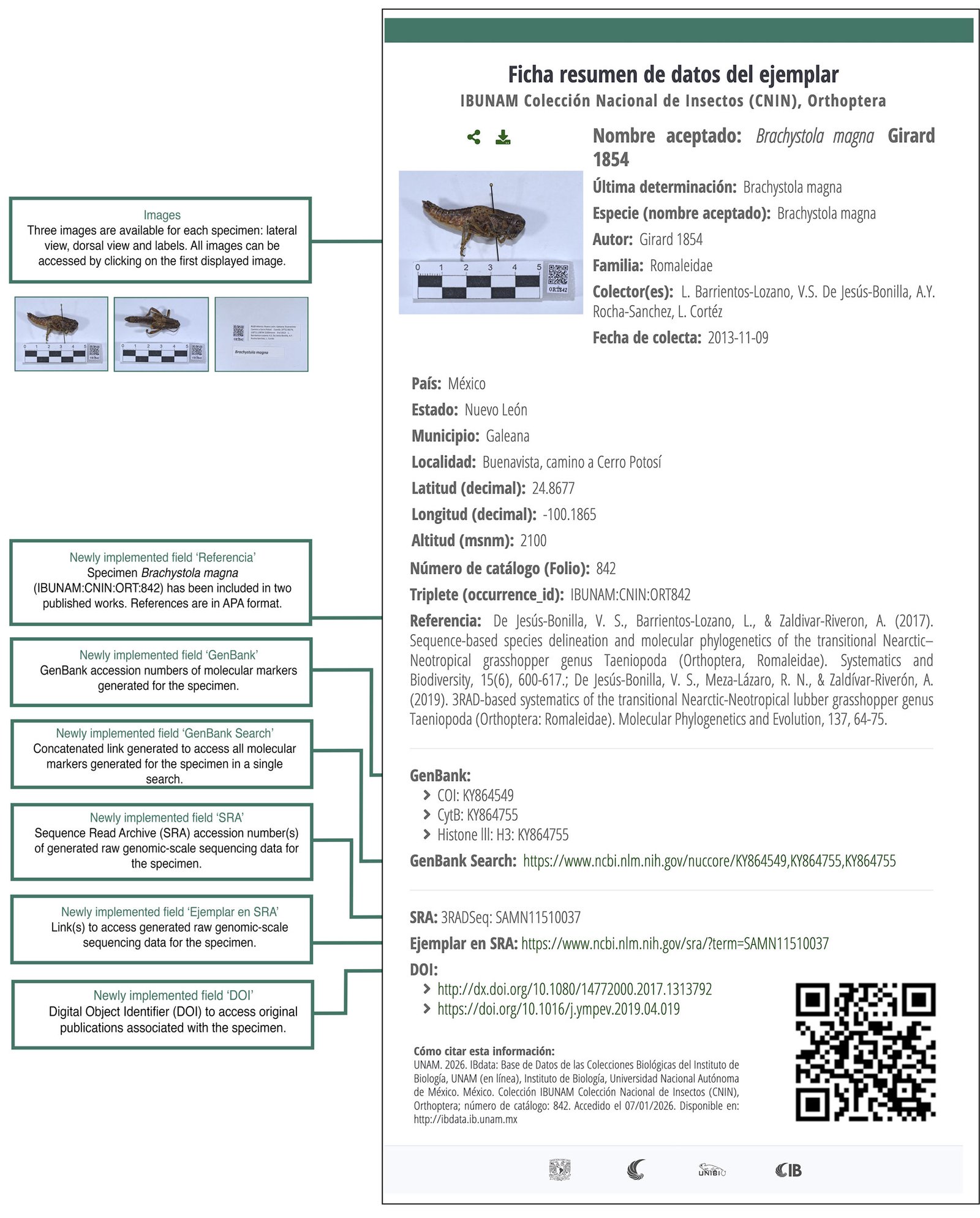
We created new fields into IBdata to capture links to accession numbers of associated genetic and genomic data as well as to the Digital Object Identifier (DOI) of original publications as follows: field ‘GenBank’ containing a list of accession numbers of all molecular markers generated for each specimen; field ‘GenBank Search’ containing a generated concatenated link to GenBank which displays all accession numbers in the field ‘GenBank’ in a single search; field ‘SRA’ containing a list of accession numbers to raw-genomic data generated for some specimens; field ‘Ejemplar en SRA’ (Spanish for ‘Specimen in SRA’) containing the direct link to raw-genomic data into the SRA database; field ‘DOI’ containing the web link to the original publication to which each specimen is associated and field ‘Referencia’ (Spanish for ‘Reference’) with the reference(s) in APA format.
We imaged dorsal and lateral views of each specimen as well as their labels, all images including the previously generated and printed QR codes. In order to do this, we used a Canon EOS Mark II camera with a 50 mm lens on a stand with side light spotlights. We developed a custom automated tool installed locally to verify for images quality, format, size, and image files integrity. This system also enables automatic renaming of image files by reading QR codes included at the time of images capture, thereby minimizing manual processing during large-scale digitization. Images are subsequently and automatically converted to format WebP through the system to optimize storage without loss of images quality. After renaming and validation, the 3 images generated for each specimen were imported into IBdata and can be accessed both as a direct IBdata search or by scanning the pinned QR label.
Results
As a result of an exhaustive navigation of the Orthoptera subcollection, we located material belonging to 36 species whose type material (holotypes, paratypes) is deposited in the CNIN, representative of the families Acrididae, Gryllidae, Pyrgomorphidae, Stenopelmatidae and Tettigoniidae (Table 1). Seven species have only paratypes deposited in the CNIN, and their respective holotypes are deposited either in the Academy of Natural Sciences of Philadelphia (ANSP), USA or in the Museo Civico di Rovereto (MCRI), Italy (Table 1).
Table 1. List of type specimens deposited in the Orthoptera subcollection of the CNIN. For some species, only paratypes are deposited in the CNIN; the holotype of the species with an asterisk (*) are deposited in the Academy of Natural Sciences of Philadelphia (ANSP), USA, and the holotype of the species with 2 asterisks (**) are deposited in the Museo Civico di Rovereto (MCRI), Italy.
We identified 7 articles in which genetic and genomic data have been generated for Orthoptera specimens deposited in the CNIN-IBUNAM corresponding to the Caelifera families Pyrgomorphidae (Sphenarium spp., Sphenacris crassicornis, Prosphena scudderi) and Romaleidae (Brachystola magna, Chromacris colorata, Cibotopteryx variegata, Romalea spp.); and to the Ensifera family Stenopelmatidae (Ammopelmatus sp., Stenopelmatus spp.) (Table 2). These investigations were centered in species delimitation, generation of phylogenetic hypotheses, population genetics and taxonomic revision of these taxa. The genetic resources generated from these specimens correspond to Cytochrome Oxidase Subunit I (COI), Cytochrome B (CytB), 28S ribosomal RNA, and Histone III (H3). For 200 of these specimens genomic-level data was generated, including low-coverage shotgun sequencing data, Triple-digest Restriction Associated DNA sequencing (3RADseq) and partial or complete mitochondrial genomes (Table 2).
Original reference
Species included
Number of specimens
Genetic and genomic data generated and publicly available
Genetic: COI Genomic: mitogenomes, 3RADseq, low-coverage shotgun sequencing data
Table 2. Orthoptera species and number of specimens in CNIN with genetic and genomic data associated.
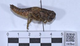
As result of digitization of type specimens and those with genetic data associated, the virtual Orthoptera collection in IBdata currently contains 610 records, from which 485 have Summary Data Sheets containing the 6 newly implemented fields integrating accession numbers, links to NCBI (GenBank and SRA), references and DOIs of original publications (Fig. 1).
Figure 1. Example of Summary Data Sheet in IBdata of Brachystola magna with catalog number 842 (URN = IBUNAM:CNIN:ORT842) including the newly implemented fields to integrate genetic and genomic resources as well as references and DOIs of original associated publications.
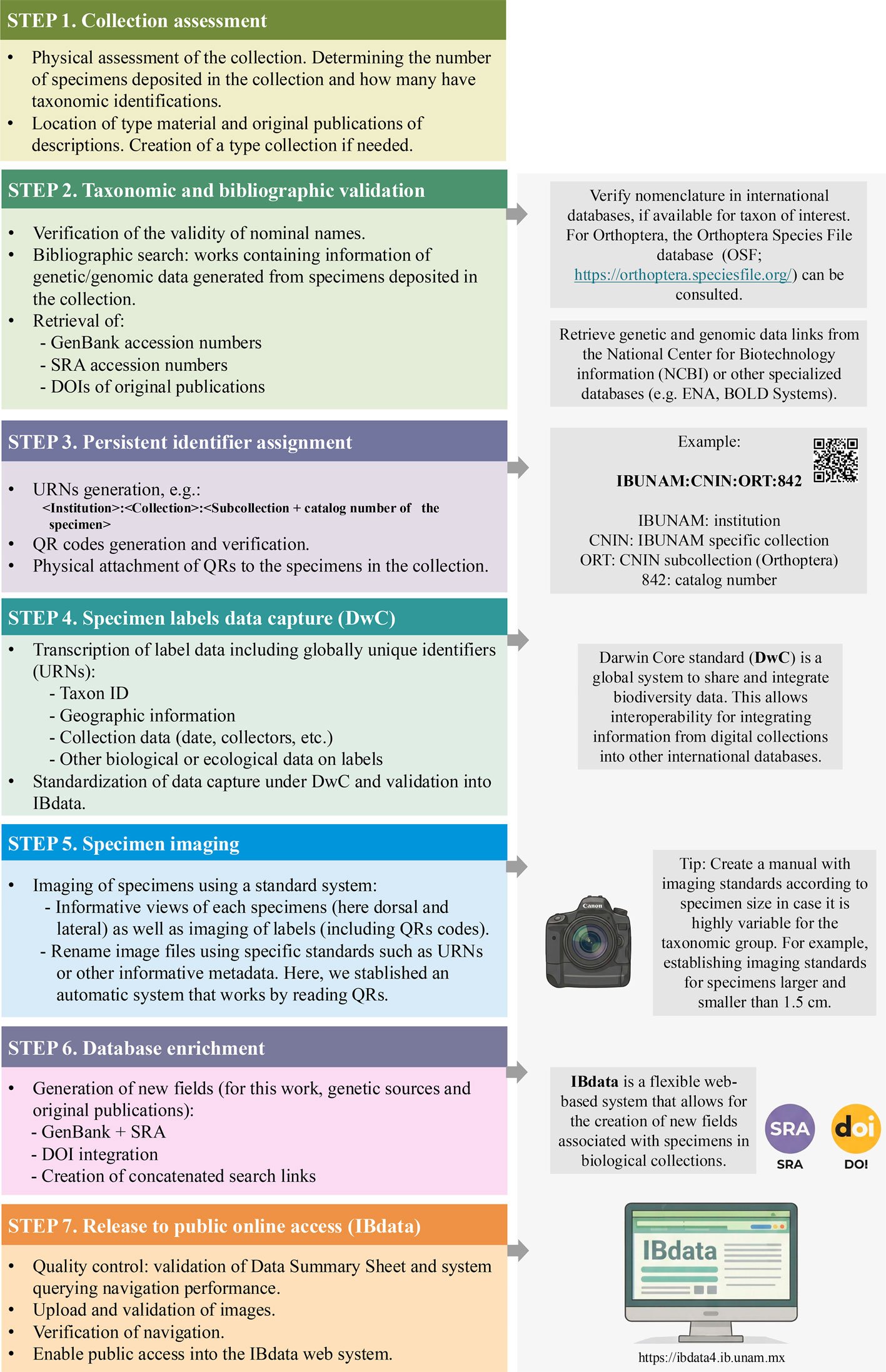
We also generated a 7-phase workflow (Fig. 2) that summarizes the methods applied here, and that can serve as a basic step-by-step guide for users associated not only to IBUNAM collections, but that are interested in initiating or enriching digitization of biological collections in other institutions. Briefly, the workflow includes: 1) initial collection assessment, 2) taxonomic and bibliographic validation, 3) persistent identifier assignment, 4) label data transcription and database capture complying with Darwin Core (DwC), 5) specimens imaging, 6) database enrichment, in the case of this study, genetic information linked to specimens in the collection, and 7) release to public online access (Fig. 2).
Figure 2. Generalized workflow for specimens digitization, validation, enrichment and online access to associated data.
Discussion
In this work, 610 new records of Orthoptera specimens collected in Mexico are now available for public consultation, which together with other virtual entomological collections with Orthoptera records, e.g., National Museum of Natural History of the Smithsonian Institution and the Natural History Museum of London, represent important contributions for opening access to Orthoptera information from Mexico and other parts of the world.
The Orthoptera subcollection of the CNIN is currently the only zoological virtual collection in IBdata that contains genetic and genomic data associated in this institutional database, and the only biological collection housed by the IBUNAM that contains associated DOIs to original publications where these specimens have been studied. This effort for enriching the institutional database IBdata is not isolated, there is an important previous initiative that linked genetic resources to type material of the National Herbarium of Mexico (MEXU) (Granados-Mendoza et al., 2024). Considering that the IBUNAM has implemented its own database for managing its biological collections comprising 10 Zoological Collections and the herbarium MEXU, most of which are reference collections in Mexico, this approach can serve as a model for institutional digitization.
The advent of next-generation sequencing technologies (NGS) has increased the production of molecular data from specimens that are subsequently deposited in biological collections, becoming an extension of these preserved specimens and transforming biological collections into dynamic resources of integrative data. Standardized approaches for linking these genetic resources to other data associated with specimens is critical to the enhancement of the scientific value of specimens and collections. In this sense, the adoption of the Darwin Core standard (DwC), a global system to share and integrate biodiversity data (Wieczorek et al., 2012) by the institutional web system IBdata, is crucial to enhance accessibility and long-term value of biodiversity data, enabling interoperability and the integration of its records into major global biodiversity infrastructures such as the Global Biodiversity Information Facility (GBIF: https://www.gbif.org/). This facilitates the incorporation of information of the IBUNAM institutional biodiversity database into large-scale studies, including monitoring of biodiversity, analysis on the impacts of climate change, ecological, phylogenetic and biogeographic studies, as well as meta-analyses.
Revision of specimens in biological collections and digitization of their associated data facilitates assessment of the state of collections and to optimally plan efforts to enhance their preservation and resources allocation (Beaman & Cellinese, 2012; Hedrick et al., 2020). Positively, digitization efforts of Mexican fauna, including insects, are increasing (e.g., Cubillos-Macías et al., 2025; Pinedo-Escatel et al., 2025), which is helping to democratize biological knowledge. In this context, the inclusion of other resources that are valuable extensions of preserved specimens such as genetic and genomic resources as a standard is critical, considering the current global biodiversity loss scenarios.
Acknowledgements
We thank Maryangela Rodríguez-Hamilton for her help with transcription of specimen labels data in an earlier stage of this study, Isabela Midori Watanabe and Alejandro Zaldívar-Riverón for their help verifying data associated with some specimens. I. Cubillos-Macías thanks the Graduate Program in Biological Sciences of the Universidad Nacional Autónoma de México (UNAM) for the support provided during his master’s studies. This work was supported by the institutional (IBUNAM) project PRONAII-2024-3 (Secihti, México), by a Secihti grant (Ciencia y Frontera 2025, project No. CBF-2025-I-21) to JMJM, and grants given by DGAPA-UNAM (PAPIIT, 2025; project No. IA201425) to JMJM and (PAPIIT, 2026; project No. IF200926) to CMM.
References
Beaman, R. S., & Cellinese, N. (2012). Mass digitization of scientific collections: new opportunities to transform the use of biological specimens and underwrite biodiversity science. Zookeys, 209, 7. https://doi.org/10.3897/zookeys.209.3313
Benites, P., Zaldívar-Riverón, A., Meza-Lázaro, R. N., Samacá- Saenz, E., Gutiérrez-Rodríguez, J., & Hernández-López, A. (2023). Multiple introgression events during the diversification history of the edible Mexican grasshopper genus Sphenarium (Orthoptera: Pyrgomorphidae). Molecular Phylogenetics and Evolution, 183, 107774. https://doi.org/10.1016/j.ympev.2023.107774
Cubillos-Macías, I., Vásquez-Quintero, A. E., Murguía- Romero, M., & Jasso-Martínez, J. M. (2025). Assessment and digitization of Mantodea (Insecta) in the Colección Nacional de Insectos (CNIN) at Instituto de Biología (IBUNAM), Mexico City, Mexico. Zootaxa, 5692, 369–380. https://doi.org/10.11646/zootaxa.5692.2.9
De Jesús-Bonilla, V. S., Barrientos-Lozano, L., & Zaldívar- Riverón, A. (2017). Sequence-based species delineation and molecular phylogenetics of the transitional Nearctic– Neotropical grasshopper genus Taeniopoda (Orthoptera, Romaleidae). Systematics and Biodiversity, 15, 600–617. https://doi.org/10.1080/14772000.2017.1313792
De Jesús-Bonilla, V. S., Meza-Lázaro, R. N., & Zaldívar- Riverón, A. (2019). 3RAD-based systematics of the transitional Nearctic-Neotropical lubber grasshopper genus Taeniopoda (Orthoptera: Romaleidae). Molecular Phylogenetics and Evolution, 137, 64–75. https://doi.org/10.1016/j.ympev.2019.04.019
Funk, V. A. (2018). Collections-based science in the 21st century. Journal of Systematics and Evolution, 56, 175–193. https://doi.org/10.1111/jse.12315
Granados-Mendoza, C., Murguía-Romero, M., & Salazar, G. A. (2024). It’s time to celebrate! Linking genetic resources to the Mexican National Biological Collections custodied by the Institute of Biology of the National Autonomous University of Mexico. Revista Mexicana de Biodiversidad, 95, e955509. https://doi.org/10.22201/ib.20078706e.2024.95.5509
Gutiérrez-Rodríguez, J., Zaldívar-Riverón, A., Weissman, D. B., & Vandergast, A. G. (2022). Extensive species diversification and marked geographic phylogenetic structure in the Mesoamerican genus Stenopelmatus (Orthoptera: Stenopelmatidae: Stenopelmatinae) revealed by mitochondrial and nuclear 3RAD data. Invertebrate Systematics, 36, 1–21. https://doi.org/10.1071/IS21022
Hedrick, B. P., Heberling, J. M., Meineke, E. K., Turner, K. G., Grassa, C. J., Park, D. S. et al. (2020). Digitization and the future of natural history collections. Bioscience, 70, 243–251. https://doi.org/10.1093/biosci/biz163
Lendemer, J., Thiers, B., Monfils, A. K., Zaspel, J., Ellwood, E. R., Bentley, A. et al. (2020). The extended specimen network: A strategy to enhance US biodiversity collections, promote research and education. Bioscience, 70, 23–30. https://doi.org/10.1093/biosci/biz140
Meineke, E. K., Davies, T. J., Daru, B. H., & Davis, C. C. (2019). Biological collections for understanding biodiversity in the Anthropocene. Philosophical Transactions of the Royal Society B, 374. https://doi.org/10.1098/rstb.2017.0386
Murguía-Romero, M., Serrano-Estrada, B., Salazar, G. A., Sánchez-González, G. E., Samper-Palacios, U. M., Gernandt, D. S. et al. (2024). The IBdata web system for biological collections: design focused on usability. Biodiversity Informatics, 18, 1–12. https://doi.org/10.17161/bi.v18i.20516
Pedraza-Lara, C., Barrientos-Lozano, L., Rocha-Sánchez, A. Y., & Zaldívar-Riverón, A. (2015). Montane and coastal species diversification in the economically important Mexican grasshopper genus Sphenarium (Orthoptera: Pyrgomorphidae). Molecular Phylogenetics and Evolution, 84, 220–231. https://doi.org/10.1016/j.ympev.2015.01.001
Pinedo-Escatel, J. A., Blanco-Rodríguez, E., Jarillo, A. M., Becerra-Chiron, I. M., Torres-Moreno, R., Vega- Ovando, F. R. et al. (2025). Annotated type catalogue of the leafhoppers and treehoppers (Insecta: Hemiptera: Auchenorrhyncha) deposited in the collection of Instituto Nacional de Investigaciones Forestales, Agrícolas y Pecuarias, Guanajuato, Mexico. Zootaxa, 5691, 151–192. https://doi.org/10.11646/zootaxa.5691.2.1
Ruiz-Mendoza, P. X., Jasso-Martínez, J. M., Gutiérrez-Rodríguez, J., Samacá-Sáenz, E., & Zaldívar-Riverón, A. (2023). Mitochondrial genome characterization and mitogenome phylogenetics in the central Mexican Stenopelmatus talpa complex (Orthoptera: Stenopelmatidae: Stenopelmatini). Revista Mexicana de Biodiversidad, 94, e945094. https://doi.org/10.22201/ib.20078706e.2023.94.5094
Saint-Andre, P., & Klensin, J. (2017). Uniform Resource Names (URN), namespace definition mechanisms. Internet Engineering Task Force (Technical report), RFC 8141.
Suastes-Jiménez, M. Á., Barrientos-Lozano, L., Gutiérrez- Rodríguez, J., Jasso-Martínez, J. M., & Zaldívar-Riverón, A. (2023). Taxonomic revision of the Stenopelmatus talpa species group (Orthoptera: Stenopelmatidae: Stenopelmatini). Revista Mexicana de Biodiversidad, 94, e945184. https://doi.org/10.22201/ib.20078706e.2023.94.5184
Wieczorek, J., Bloom, D., Guralnick, R., Blum, S., Döring, M., Giovanni, R. et al. (2012). Darwin Core: an evolving community-developed biodiversity data standard. Plos One, 7, e29715. https://doi.org/10.1371/journal.pone.0029715
Biogeography of an invasion: distribution, biases and expansion of Linepithema humile in Mexico
Diego López-Collar a, César Maximiliano Vázquez-Franco b, Diego Gil-Tapetado c y Tania Escalante d, *
a Universidad Complutense de Madrid, Facultad de Ciencias Biológicas, Departamento de Biodiversidad, Ecología y Evolución, Grupo de Biología Evolutiva y de la Conservación, Ciudad Universitaria, C/ José Antonio Novais, 12, Moncloa-Aravaca, 28040 Madrid, España b Universidad Nacional Autónoma de México, Facultad de Ciencias, Departamento de Biología Evolutiva, Museo de Zoología “Alfonso L. Herrera”, Circuito Exterior s/n, Ciudad Universitaria, 04510 Ciudad de México, México c Universidad de Murcia, Campus Espinardo, Facultad de Biología, Departamento de Ecología e Hidrología, 30100 Murcia, España d Universidad Nacional Autónoma de México, Facultad de Ciencias, Departamento de Biología Evolutiva, Grupo de Biogeografía de la Conservación, Circuito Exterior s/n, Ciudad Universitaria, 04510 Ciudad de México, México
*Autor para correspondencia: tescalante@ciencias.unam.mx (T. Escalante)
Recibido: 14 mayo 2025; aceptado: 1 junio 2026
Resumen
Linepithema humile (Mayr, 1868), es una de las especies invasoras más dañinas a escala global. En este estudio analizamos su distribución en México mediante un enfoque areográfico y temporal y modelamos su distribución potencial a partir de la literatura científica, colecciones biológicas y plataformas de ciencia ciudadana. Asimismo, evaluamos el grado de expansión urbana y la presencia de supercolonias en la Ciudad de México. La especie se registró en 14 estados y 15 ecorregiones, con una alta concentración en la Ciudad de México y áreas del centro del país y presencias dispersas en otros entornos urbanos. Encontramos un aumento pronunciado de registros desde 2015, impulsado por las plataformas de ciencia ciudadana. Los modelos de distribución potencial predicen una alta idoneidad ambiental en Baja California y en la Faja Volcánica Transmexicana, especialmente en zonas urbanizadas. En la Ciudad de México, L. humile ocupó 13 alcaldías y los ensayos de agresividad indicaron la existencia de una única supercolonia. Los resultados destacan el papel de la urbanización en la dinámica de invasiones, la necesidad de abordar los sesgos asociados a la procedencia de los datos y el valor de la ciencia ciudadana para el monitoreo de esta especie.
Palabras clave: Ciencia ciudadana; Distribución geográfica; Especie exótica; Formicidae; Supercolonia
Abstract
Linepithema humile (Mayr, 1868), is one of the most damaging invasive species worldwide. We analyzed its distribution in Mexico using an areographic and temporal approach, and modeled its potential distribution based on records from scientific literature, biological collections, and citizen science platforms. In addition, we assessed its degree of urban occupancy and the presence of supercolonies in Mexico City. The species was recorded in 14 states and 15 ecoregions, with a high concentration in Mexico City and adjacent areas of central Mexico, and scattered occurrences elsewhere, primarily in urban environments. Records showed a pronounced increase since 2015, in part driven by citizen science platforms. Potential distribution models predicted high environmental suitability in Baja California and the Trans-Mexican Volcanic Belt, particularly in urbanized areas. In Mexico City, L. humile occupied 13 boroughs, and aggression assays indicate the presence of a single supercolony. Our results emphasize the central role of urbanization in invasion dynamics, the need to address biases associated with data origin and highlight the value of citizen science for monitoring this species.
Linepithema humile (Mayr, 1868), conocida comúnmente como la hormiga argentina, en referencia al país donde se recolectaron los ejemplares utilizados para su descripción (Mayr, 1868; Newell y Barber, 1913), ha adquirido una notable relevancia debido a los impactos ecológicos que genera fuera de su área de distribución nativa (Wetterer et al., 2009), lo que ha motivado su inclusión entre las 100 especies invasoras más perjudiciales a escala global (Global Invasive Species Database, 2009).
El establecimiento de L. humile fuera de su área de distribución natural provoca impactos negativos significativos sobre las comunidades nativas de hormigas (Holway et al., 2002; Menke et al., 2018; Zina et al., 2020) y otros artrópodos (Stanley y Ward, 2012), además de alterar múltiples interacciones ecológicas, con efectos en cascada sobre vertebrados y relaciones planta-animal (Álvarez-Blanco et al., 2017; Blancafort y Gómez, 2005; Gómez y Abril, 2008; Gómez y Oliveras, 2003; Suarez y Case, 2002). Asimismo, L. humile presenta una marcada capacidad para establecerse en entornos alterados antropogénicamente (Holway y Suarez, 2006; Stringer et al., 2009; Touyama et al., 2003), donde constituye un problema relevante al generar pérdidas económicas asociadas a daños en infraestructuras, molestias en propiedades privadas y, especialmente, impactos en el sector agrícola, en gran medida vinculados a su relación mutualista con plagas agrícolas del suborden Sternorrhyncha (Aphididae y Coccoidea) (Gómez y Abril, 2008; Harris, 2002; Newell y Barber, 1913; Suzuki et al., 2025; Zina et al., 2020). En conjunto, estas características dificultan los programas de control y erradicación, que requieren una elevada inversión de recursos y planificación a largo plazo (Angulo et al., 2022, 2024).
Linepithema humile es originaria de la región subtropical de América del Sur, con una distribución nativa asociada a la cuenca del río Paraná (Wetterer et al., 2009). Sin embargo, esta hormiga se ha expandido ampliamente a escala global como consecuencia de la actividad humana, principalmente a través del transporte de mercancías y el comercio internacional (Angulo et al., 2024; Queiroz y Alves, 2018). En la actualidad, L. humile se encuentra ampliamente distribuida en regiones templadas y subtropicales en todo el mundo, incluyendo extensas áreas del sur de Europa, el sureste y la costa oeste de los EUA, algunas localidades en Japón, el suroeste y sureste de Australia, Nueva Zelanda, Sudáfrica y amplias regiones de América Central y del Sur, además de diversos archipiélagos e islas, como Azores, Canarias o Hawai entre otras (Guénard et al., 2017; Wetterer et al., 2009).
La vía de introducción de esta hormiga invasora en México no es clara; sin embargo, se ha propuesto que su llegada estuvo asociada al comercio internacional, mediante la importación de productos procedentes de su área nativa o de otras regiones previamente invadidas (Rosas-Mejía y Janda, 2017), un patrón coherente con lo observado a escala global (Queiroz y Alves, 2018; Roura-Pascual et al., 2009; Suarez et al., 2001; Wetterer et al., 2009). Ante la ausencia de evidencias de dispersión natural secundaria, se plantea que su expansión dentro del territorio mexicano ha estado mediada principalmente por la actividad humana (Rosas-Mejía y Janda, 2017), tal como se ha documentado en otras regiones del mundo (Roura-Pascual et al., 2009; Ward et al., 2005). Actualmente, L. humile está catalogada como especie no nativa invasora en México y forma parte del listado de 42 especies no nativas registradas para el país (Bolton, 2024; DOF, 2016; Rosas-Mejía et al., 2021). Asimismo, ha sido evaluada mediante el método de evaluación rápida de invasividad (MERI), en el que se le asigna un riesgo de invasividad y de dispersión muy elevado (Conabio, 2016).
El potencial invasor de L. humile ha sido revisado por diversos autores mediante modelos de nicho ecológico y de distribución potencial, evidenciando, para la región Neártica, una marcada afinidad por territorios meridionales, como la costa del Golfo de México, así como por la costa oeste de los EUA (Hartley et al., 2006; Jung et al., 2022; Li et al., 2024; Roura-Pascual et al., 2004). En el caso de México, estos modelos identifican áreas con elevada idoneidad climática en la península de Baja California, las zonas elevadas de la Faja Volcánica Transmexicana y la península de Yucatán (Jung et al., 2022; Roura-Pascual et al., 2011). A escala global, un rasgo recurrente en las regiones invadidas por la especie es la alta idoneidad de las áreas costeras, donde la influencia marítima atenúa la continentalidad, incrementa la humedad ambiental y suaviza los extremos térmicos (López-Collar et al., 2024; Roura-Pascual et al., 2011). No obstante, persisten importantes lagunas en la comprensión de los patrones de idoneidad y distribución potencial de L. humile a escalas espaciales más finas, especialmente en relación con factores antrópicos como el grado de urbanización, que se ha demostrado determinante en la distribución de especies asociadas a ambientes perturbados (Polidori et al., 2021), incluida la propia hormiga argentina (López-Collar et al., 2024; Roura-Pascual et al., 2011).
La urbanización constituye uno de los principales motores contemporáneos a escala global de la introducción, establecimiento y expansión de especies exóticas e invasoras, al generar entornos altamente perturbados que favorecen a organismos con rasgos sinantrópicos y elevada plasticidad ecológica (Borden y Flory, 2021; McKinney, 2006). En este contexto, L. humile muestra una notable capacidad para colonizar áreas urbanas, donde la disponibilidad constante de recursos, la reducción de competidores nativos y la conectividad asociada a las infraestructuras humanas facilitan su persistencia y expansión (Holway y Suarez, 2006; Park et al., 2014). En México, las áreas urbanas concentran una proporción especialmente elevada de registros de hormigas exóticas (Rosas-Mejía et al., 2021), lo que las convierte en escenarios clave tanto para el seguimiento temprano de las invasiones biológicas como para la evaluación del grado de expansión espacial de las especies invasoras. La Ciudad de México, una de las mayores metrópolis a nivel mundial, constituye un sistema particularmente relevante para analizar la distribución local de L. humile y sus patrones de establecimiento y expansión en un entorno altamente urbanizado. Asimismo, el estudio de la invasión de esta especie permite incorporar una dimensión poblacional y de comportamiento mediante la evaluación de la existencia de supercolonias, entendidas como redes de colonias genéticamente relacionadas y carentes de agresión intraespecífica (Angulo et al., 2024; Sunamura et al., 2009). Estas estructuras sociales, cuya presencia ha sido documentada en distintas regiones del mundo (Sunamura et al., 2009; Vogel et al., 2010), están estrechamente ligadas al éxito invasor de L. humile y a la intensificación de sus impactos ecológicos, al favorecer la cooperación a gran escala, la homogeneización biótica y el desplazamiento de las comunidades nativas (Angulo et al., 2024; Blight et al., 2012; Brandt et al., 2009; Suhr et al., 2009).
La ciencia ciudadana, ya sea a través de iniciativas participativas a escala local —como School of Ants (Lucky et al., 2014), Correo Real (Rendón-Salinas et al., 2026) o el urban Butterfly Monitoring Scheme (uBMS; Guzmán et al., 2023)— o mediante plataformas globales (p. ej., eBirds.org, iNaturalist.org, Observation.org), se ha consolidado como una fuente relevante de información para el estudio y la conservación de la biodiversidad, al aportar grandes volúmenes de datos con amplia cobertura espacial y temporal (Chandler et al., 2017), complementarios a los procedentes de la literatura científica y las colecciones biológicas. Estos datos se han utilizado mayoritariamente para estimar áreas de distribución geográfica y patrones biogeográficos (Mason et al., 2025), pero también son especialmente relevantes para documentar la presencia de especies exóticas (Demetriou et al., 2025; Hiller y Haelewaters, 2019), el seguimiento de especies invasoras (Johnson et al., 2020) o la mejora de modelos de idoneidad ambiental y distribución potencial (Dimson et al., 2023). En este contexto, la ciencia ciudadana resulta particularmente relevante para monitorear especies asociadas a entornos antropizados, como es el caso de especies invasoras con comportamiento similar al de plagas (p. ej., L. humile), donde puede aumentar la probabilidad de detección y reporte por parte de la ciudadanía (Werenkraut et al., 2025). Sin embargo, la concentración de participación de observadores en áreas urbanas puede generar un sesgo espacial hacia entornos densamente poblados (Geldmann et al., 2016; Mair y Ruete, 2016). Además, persisten problemas relacionados con la calidad y consistencia de los datos, como identificaciones erróneas y sesgos taxonómicos y temporales, especialmente para especies crípticas, factores que explican la reticencia a emplear estos datos en determinados estudios si no se aplican procedimientos de validación adecuados (Burgess et al., 2017).
Ante la necesidad de abordar la invasión de L. humile en México desde un enfoque biogeográfico sintético, que combine múltiples fuentes de información, se proponen los siguientes objetivos: i) actualizar la distribución geográfica conocida de L. humile en México, ii) analizar su expansión espacial y temporal mediante un enfoque biogeográfico que integre análisis areográficos y modelos de distribución potencial. Asimismo, iii) evaluar el papel de la ciencia ciudadana en el seguimiento de la especie y la influencia de la urbanización en su proceso de invasión, considerando explícitamente los sesgos taxonómicos, espaciales y temporales asociados a las fuentes de datos. Por último, iv) evaluar el grado de expansión y la presencia de supercolonias en la Ciudad de México.
Materiales y métodos
Para el análisis areográfico y la evaluación de la expansión geográfica y temporal de L. humile en México, los registros de presencia se obtuvieron de las siguientes fuentes: i) el Global Biodiversity Information Facility (GBIF; referencia de descarga: GBIF.org, 2025a; www.GBIF.org), que aloja datos con licencia de uso explícita procedentes de la plataforma colaborativa iNaturalist (iNaturalist, 2026); ii) bases de datos especializadas en mirmecología, incluyendo Antmaps (Guénard et al., 2017; Janicki et al., 2016; www.antmaps.org;) y AntWeb (AntWeb, 2024; www.antweb.org); iii) bibliografía científica; y iv) registros adicionales obtenidos por los autores a través de comunicaciones personales y muestreos directos.
Para comprobar la fiabilidad de los datos procedentes de plataformas de ciencia ciudadana, se utilizaron los registros de iNaturalist atribuidos a la categoría de “research grade” (es decir, datos validados por la plataforma para su uso en investigación) disponibles a través de GBIF.
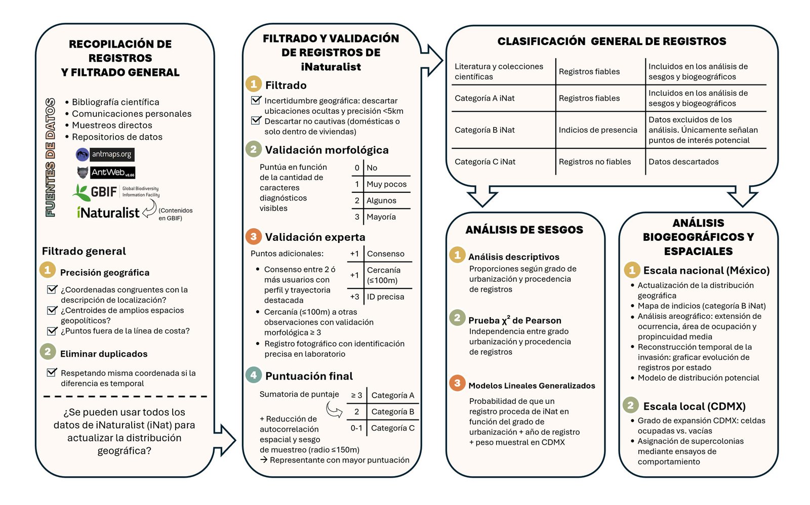
Los datos de presencia fueron sometidos a un proceso de revisión y filtrado para asegurar su fiabilidad (fig. 1). Por un lado, se constató la precisión y congruencia territorial, y se descartaron aquellos puntos correspondientes a centroides de espacios geopolíticos de grandes dimensiones geográficas (p. ej., estados), localizaciones incongruentes o situadas fuera de la línea de costa correspondiente a los límites geopolíticos de México, que no pudieran ser reasignados a localizaciones precisas por la ausencia de la descripción de las localidades. Asimismo, se descartaron registros con georreferencias duplicadas, respetando la coincidencia de coordenadas si existía diferencia temporal o suponían especímenes diferentes pertenecientes a la misma colección científica.
Figura 1. Flujo de trabajo que resume la recopilación y el filtrado de datos, el esquema de validación de registros de iNaturalist y la clasificación de los registros. También se indican los análisis realizados en paralelo: sesgos temporales y espaciales, y análisis biogeográficos a escala regional y local.
Particularmente en el caso de los datos de iNaturalist, las observaciones debían ser no cautivas (para excluir potencialmente las colonias de hormigas domésticas cuyo origen no representa una presencia natural o establecida en la zona), con ubicaciones no ocultas y una incertidumbre geográfica de menos de 5 km. Los registros de iNaturalist contenidos en GBIF (GBIF.org, 2025a) pasaron de 349 a 315 registros antes de ser sometidos al proceso de validación mostrado a continuación. Con el objetivo de realizar una selección rigurosa de los registros fotográficos que reflejara el potencial de la plataforma para detectar indicios de la presencia de L. humile, se elaboró un sistema de puntuación para categorizar la calidad científica de los datos (fig. 1).
Validación morfológica
El primer paso consistió en la valoración morfológica de los individuos fotografiados, de manera que se otorgó una puntuación en función del número de caracteres diagnóstico con base en la descripción de L. humile propuesta por Wild (2007) que fueran visibles (0-No; 1-Muy pocos; 2-Algunos; 3-Mayoría) e incluyen una combinación de escapos antenales largos, llegando a superar fácilmente el margen posterior de la cabeza en vista frontal; cabeza en vista frontal más larga que ancha, alcanzando su punto más ancho justo detrás de los ojos compuestos y estrechada en la parte anterior, con los márgenes laterales convergiendo en dirección a las mandíbulas, lo que la hace tener un aspecto triangular y alargado; en vista lateral se aprecia el pronoto y mesonoto formando una línea convexa continua con una sutura mesopropodeal algo marcada y el propodeo inclinado hacia adelante; el pronoto y los 2 primeros terguitos del gáster sin setas erectas son caracteres clave, pero difícilmente apreciables en fotografías con resolución limitada; el cuerpo y los apéndices normalmente de tonos marrón rojizo y amarillento; en ciertos casos la cabeza y gáster de un color grisáceo más oscuro que el mesosoma; gáster normalmente de color gris oscuro de forma alargada y terminado en pico; cuerpo de tamaño pequeño (2.3-3 mm) y estilizado.
Validación experta
A partir de esta puntuación inicial, se añadió un punto adicional en 2 situaciones: i) con el objetivo de incorporar el criterio experto, cuando existía consenso entre 2 o más usuarios de iNaturalist con experiencia demostrada en mirmecología, reflejada en sus perfiles mediante la afiliación a instituciones de investigación de reconocido prestigio (centros de investigación o universidades) y una trayectoria constatada en la identificación de observaciones naturalistas, que mostrara más de 10,000 identificaciones; y ii) cuando se disponía de otras observaciones con una puntuación de caracteres morfológicos igual a 3 dentro de un radio ≤ 100 m. En este último caso, se asumió la disponibilidad de un mayor número de caracteres diagnósticos visibles al tratarse de fotografías pertenecientes a un mismo conjunto de observaciones o a individuos de la misma colonia.
Asimismo, se añadieron 3 puntos a aquellas observaciones asociadas a muestras con ejemplares colectados que pudieron ser identificados paralelamente mediante una lupa binocular. Con base en la puntuación total obtenida, cada registro fue asignado a una categoría de calidad: puntuación ≥ 3 (categoría A), puntuación = 2 (categoría B) y puntuación = 0-1 (categoría C). Finalmente, con el fin de reducir la autocorrelación espacial y el sesgo asociado al esfuerzo de muestreo, las observaciones localizadas dentro de un radio ≤ 150 m fueron agrupadas y representadas por el registro de mayor categoría.
Procedencia y clasificación de los registros de presencia
A continuación, se detalla el número de registros en función de su procedencia (tabla 1), categoría de fiabilidad y aplicación en el presente estudio. Literatura y colecciones científicas: este conjunto incluye 35 registros, correspondientes a 32 georreferencias únicas de especímenes depositados en colecciones científicas y observaciones realizadas por especialistas publicadas en la literatura científica. A efectos de este estudio, estos registros presentan el máximo nivel de fiabilidad, dado que su procedencia garantiza una correcta identificación taxonómica. Por ello, fueron utilizados para los análisis biogeográficos, la evaluación de sesgos y los modelos de distribución potencial. Categoría A (iNaturalist): estos 65 registros, correspondientes a 125 observaciones tras la eliminación de la autocorrelación espacial, se basan en fotografías de calidad suficiente, en las que la postura de los individuos permite reconocer de forma inequívoca la combinación de caracteres diagnósticos suficiente para su correcta identificación, generalmente incluyendo vistas lateral y dorsal, y en algunos casos frontal. Estos datos, junto con los de literatura y colecciones científicas se utilizaron para los análisis biogeográficos, la evaluación de sesgos y los modelos de distribución potencial. Categorías B y C (iNaturalist): debido a la imposibilidad de observar con claridad los caracteres diagnósticos y a la ausencia de consenso experto, 190 registros asociados a fotografías no fueron considerados para su uso directo en investigación. En consecuencia, estos registros fueron excluidos de los análisis biogeográficos. No obstante, los registros de la categoría B (55 observaciones no autocorrelacionadas espacialmente) se emplearon para señalar puntos de interés (p. ej., con vistas a futuras campañas de muestreo) y deben interpretarse únicamente como indicios de la posible presencia de L. humile.
Tabla 1. Número de registros antes y después del proceso de filtrado y validación atendiendo al ámbito geográfico y de análisis. CDMX: Ciudad de México; MDP: modelo de distribución potencial; GBIF: Global Biodiversity Information Facility; Coord.: coordenadas; FAE: filtro de autocorrelación espacial; des.: descartados.
Análisis areográfico y reconstrucción temporal de la invasión
Con base en los datos, se elaboró un mapa de distribución de L. humile en México con registros validados pertenecientes a la literatura, colecciones científicas y la categoría A (iNaturalist), así como un mapa de indicios complementario representando los registros de la categoría B (material suplementario 1: fig. S1) mediante QGIS Desktop 3.44.5 (QGIS.org, 2025).
Para el análisis areográfico, los registros procedentes de la literatura, colecciones científicas y categoría A se superpusieron geográficamente a los estados geopolíticos de México, las ecorregiones (Olson et al., 2001) y un mapa de vegetación y cambio de uso de suelo (INEGI, 2023). Además, los registros obtenidos fueron utilizados para reconstruir el área de distribución geográfica conocida mediante 3 procedimientos: extensión de presencia, área de ocupación (IUCN, 2019) y propincuidad media (Rapoport, 1975). Los 2 primeros métodos fueron obtenidos en QGIS con las herramientas de mínima geometría delimitadora y calculadora de malla. El método de propincuidad media fue obtenido con las medidas de la media y desviación estándar, empleando la librería “fossil” (Vavrek, 2011) en RStudio 2025.09.2+418 (Posit team, 2025) y la herramienta de agregar atributos de geometría, estadísticas para campos y buffer en QGIS.
Para reconstruir temporalmente la invasión de L. humile en los estados geopolíticos de México, se graficó el número de registros por año y en función de su procedencia (literatura y colecciones científicas o categoría A). Asimismo, se graficaron los registros acumulados por año para observar la progresión en la detección de L. humile. Para reconstruir la invasión de manera visual en el espacio geográfico se empleó la herramienta “Temporal” en QGIS para construir los 61 cuadros (1 por año de 1965 a 2025). Posteriormente, fueron usados para elaborar un GIF y un archivo de video (extensión mp4) en Ezgf.com (ezgif.com).
Análisis del sesgo de urbanización y procedencia de los datos
Para evaluar posibles sesgos asociados al grado de urbanización y a la procedencia de los registros, se clasificaron todas las observaciones en 3 categorías de tamaño poblacional humano como “proxy” del nivel de urbanización de acuerdo con la base de datos Gridded Population of the World (GPW), correspondiente al año 2015 (CIESIN-CIAT, 2024): rural (< 250 habitantes/km²), periurbano (> 250 habitantes/km²) y urbano (≥ 1,000 habitantes/km²). En primer lugar, se exploraron diferencias en el número de registros entre categorías de urbanización y respecto a la procedencia de los datos (literatura/colecciones científicas o iNaturalist), tanto a nivel general sobre el conjunto de datos como por cada estado, mediante análisis descriptivos. Además, la asociación entre la categoría de población humana y la procedencia de los registros se evaluó mediante una prueba de independencia χ² de Pearson. Posteriormente, se ajustaron modelos lineales generalizados (GLM) con distribución binomial y enlace logit para modelar la probabilidad de que un registro procediera de iNaturalist, en lugar de literatura o colecciones científicas en función de la categoría de población. Para controlar el efecto del incremento temporal del uso de plataformas de ciencia ciudadana, se incorporó el año de registro como covariable continua, previamente centrada. Dado el fuerte peso muestral de Ciudad de México, se realizaron análisis de sensibilidad excluyéndola, con el fin de evaluar la robustez de los resultados frente a la concentración espacial de registros.
Modelado de la distribución potencial
Este modelo (MDP) se utilizó para revelar áreas susceptibles de albergar la presencia de L. humile, basándose en la idoneidad del hábitat en función de variables climáticas y de urbanización. El modelo se construyó a partir de registros globales de presencia de L. humile obtenidos de GBIF (GBIF.org, 2025b) y correspondientes únicamente a datos de colecciones científicas, evitando el posible sesgo taxonómico de los datos de ciencia ciudadana a escala mundial. Tras eliminar los duplicados y referencias dudosas el número de registros se redujo de 5,993 a 1,874 (tabla 1). Los registros de México se actualizaron con los 100 registros procedentes de la literatura, colecciones científicas y categoría A empleados en el presente trabajo. Para reducir la autocorrelación espacial y el sesgo de muestreo, se realizó un filtrado espacial de 1 km² siguiendo a López-Collar et al. (2024). El conjunto definitivo quedó constituido por 1,344 registros de presencia a escala global, contando con 80 georreferencias para México (tabla 1).
La distribución potencial basada en la idoneidad del hábitat se estimó mediante el paquete sabinaNSDM (Mateo et al., 2024). Para representar la distribución completa de la especie a escala global (modelo global) y en México (modelo nacional, equivalente al modelo regional en el marco metodológico de Mateo et al. [2024]), se llevó a cabo un modelo jerárquico anidado a una resolución de 30 segundos de arco (~ 1 km²), obteniéndose modelos adicionales que incorporaron el modelo global como covariable (modelo con covariable). Los algoritmos empleados fueron: modelo aditivo generalizado (GAM), modelo lineal generalizado (GLM), gradient boosting model (GBM), random forest (RF) y el GLM ajustado mediante máxima entropía (MaxNet). Un modelo consenso final se construyó basado en el promedio de 75 modelos individuales con covariable (es decir, 15 iteraciones × 5 algoritmos).
Para el “background” se construyeron 10,000 puntos mediante la función NSDM.FormattingData del paquete sabinaNSDM (Mateo et al., 2024) y la evaluación interna se llevó a cabo mediante el área bajo la curva ROC (AUC), el true skill statistic (TSS) y el coeficiente kappa de Cohen (Kappa) para cada modelo individual y para el modelo final. La importancia relativa de cada variable y algoritmo se calculó para el modelo nacional ensamblado y para el modelo global como covariable utilizando los paquetes sabinaNSDM y biomod2 (Mateo et al., 2024). El modelo ensamblado final con covariable se convirtió en un modelo binario de presencia/ausencia utilizando el umbral de corte (0.261) que maximizó el TSS (fig. S2).
Las 19 variables bioclimáticas se obtuvieron del conjunto de datos WorldClim 2.1 (Fick y Hijmans, 2017; http://www.worldclim.org), con un tamaño de celda de 30 arcosegundos (~ 1 km²). Además, se utilizó la densidad de población humana como “proxy” del grado de urbanización proporcionada por GPW correspondiente al año 2015 (CIESIN-CIAT, 2024) para explorar la relación de L. humile con el entorno urbano.
Para establecer un conjunto de variables climáticas no correlacionadas, se caracterizaron las variables con los puntos de “background”, se realizó un análisis de correlación y, posteriormente, se eliminó una variable de cada par que presentaba un coeficiente de correlación de Pearson > 0.7. Después, se aplicó un análisis iterativo del factor de inflación de la varianza (VIF) (Lin et al., 2011) para eliminar aquellas variables con VIF > 5 que pudieran aportar información redundante al modelo (material suplementario 1: fig. S3). Finalmente, se utilizó la función NSDM.SelectCovariates del paquete sabinaNSDM (Mateo et al., 2024) para reducir el número de variables a las más relevantes para el modelo. Los MDP fueron realizados en R 4.5.0 y RStudio 2025.09.2+418. La visualización de los mapas de idoneidad se llevó a cabo mediante QGIS.
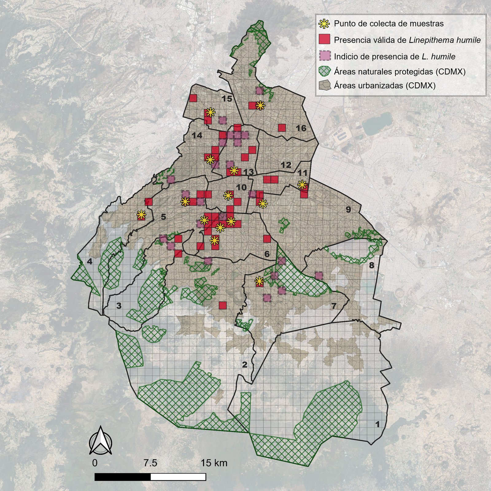
Para reflejar el grado de expansión en la Ciudad de México se tuvieron en cuenta aquellos registros pertenecientes a la literatura, colecciones científicas e iNaturalist ubicados dentro de los límites geopolíticos de las alcaldías (INEGI, 2020a). Con el propósito de sistematizar el seguimiento a largo plazo de la hormiga argentina en la Ciudad de México y evitar el sesgo de muestreo, se creó una malla de 1 km² y se asignaron los puntos a los cuadros correspondientes, distinguiendo aquellos pertenecientes a literatura, colecciones y categoría A de aquellos indicios pertenecientes a la categoría B. Como referencia espacial se añadió la capa de área geoestadística básica urbana y las áreas naturales protegidas de la ciudad (Conabio, 2020; INEGI, 2019).
Ensayos de comportamiento para la asignación de supercolonias
Sobre el mapa de la Ciudad de México, se delimitaron zonas para la búsqueda y recolección de L. humile, priorizando localizaciones previamente conocidas o áreas adyacentes, con distancias entre puntos superiores a 1 km para garantizar la independencia e identidad de cada nido. En cada sitio, se recolectaron aproximadamente entre 30 y 70 obreras, las cuales fueron mantenidas vivas en recipientes plásticos circulares (8 cm de alto y 5 cm de diámetro) con tapas perforadas para permitir la ventilación. Siempre que fue posible, se incluyó parte del sustrato del nido o, en su defecto, torundas de algodón humedecido para asegurar la supervivencia temporal de los especímenes. Parte de las muestras fueron preservadas en etanol 96º y depositadas en la Colección de Entomología de la Universidad Complutense de Madrid (UCME). Los sitios de colecta se representaron sobre el mapa de la Ciudad de México (fig. 8). Se tomaron las consideraciones pertinentes en relación con el manejo responsable de fauna silvestre, en primer lugar, contando con los permisos de colecta necesarios emitidos por la Subsecretaría de Política Ambiental y Recursos Naturales de la Dirección General de Vida Silvestre con el oficio Nº SGPA/DGVS/10697/23 y, en segundo lugar, recibiendo la aprobación por parte de la Comisión de Ética Académica y Responsabilidad Científica (CEARC/Bioética/1190226) de la Facultad de Ciencias de la Universidad Nacional Autónoma de México.
Figura 8. Mapa de las localizaciones de Linepithema humile en la Ciudad de México. Los cuadros rojos indican presencias válidas, cuyos datos proceden de literatura, colecciones científicas y registros válidos de iNaturalist (categoría A). Los cuadros rosas con línea punteada indican indicios de presencia (categoría B de iNaturalist). Las estrellas amarillas indican los puntos de colecta de muestras utilizadas en los ensayos de agresividad. La malla verde indica porciones de áreas naturales protegidas dentro de la Ciudad de México. En marrón, dentro de los límites de las alcaldías, aparece el área geoestadística básica urbana (entorno urbanizado). Las alcaldías de la ciudad se muestran en línea sólida: 1- Milpa Alta, 2 – Tlalpan, 3 – Magdalena Contreras, 4 – Cuajimalpa de Morelos, 5 – Álvaro Obregón, 6 – Coyoacán, 7 – Xochimilco, 8 – Tláhuac, 9 – Iztapalapa, 10 – Benito Juárez, 11 – Iztacalco, 12 – Venustiano Carranza, 13 – Cuauhtémoc, 14 – Miguel Hidalgo, 15 – Azcapotzalco, 16 – Gustavo A. Madero.
Los enfrentamientos individuales se llevaron a cabo en laboratorio siguiendo un protocolo estandarizado que permite la detección de diferentes supercolonias (i.e.: diferentes linajes genéticos) con un grado muy alto de fiabilidad (Blight et al., 2017; Giraud et al., 2002; Sunamura et al., 2009; Vogel et al., 2010). En placas Petri de 5.2 cm de diámetro, se colocaron 2 obreras de diferentes localidades y se observaron durante 10 minutos, registrando si ocurría una interacción de agresión, amistosa o ausencia de contacto. Una agresión implica el reconocimiento de los pares de individuos como pertenecientes a supercolonias distintas y una interacción amistosa como el reconocimiento de la misma supercolonia (Blight et al., 2017; Giraud et al., 2002; Suhr et al., 2009). Para cada par de localizaciones se establecieron 5 repeticiones de enfrentamientos individuales con obreras diferentes. Los detalles metodológicos adicionales y el material suplementario están disponibles en el repositorio en línea en: https://zenodo.org/records/21844722.
Resultados
Proceso de filtrado y validación de registros
Del total de 349 registros asociados a fotografías procedentes de iNaturalist albergados en GBIF a fecha de 06 de diciembre de 2025, 224 (64%) no superaron el filtro impuesto. La mayoría de los registros descartados se debieron a la imposibilidad de evaluar adecuadamente los caracteres diagnósticos necesarios para la correcta identificación de L. humile. Esto ocurrió principalmente por la baja resolución de las fotografías, la excesiva distancia entre la cámara y el ejemplar, o la posición desfavorable del organismo en la imagen —ya fuera por el ángulo de captura o por la ocultación parcial de estructuras corporales relevantes. En otros casos, la determinación taxonómica inicial resultó errónea debido a confusiones con taxones morfológicamente similares, como ejemplares pertenecientes a los géneros Azteca Forel, 1878 y Dorymyrmex Mayr, 1866.
Por su parte, los datos provenientes de la literatura y colecciones científicas se actualizaron tras su revisión, resultando en un total de 35 registros, de los cuales 32 están asociadas a georreferencias únicas. Por ejemplo: la cita de L. humile en Baja California reportada por Johnson y Ward (2002), presenta una imprecisión geográfica que se ha reproducido en trabajos posteriores (Dáttilo et al., 2019) y en bases de datos como GABI (Guénard et al., 2017). Dado que en dicho estado la especie se restringía a la Provincia Florística de California, es posible que el registro corresponda al entorno urbano o al municipio de Ensenada, coherente con la descripción original de la localidad, aunque no con las coordenadas que fueron asignadas posteriormente. En el caso del estado de Chihuahua, existe un registro cuya validez es incierta, ya que, aunque su presencia se refleja en Antmaps (Guénard et al., 2017) como un registro de museo, no se especifica la localidad exacta ni la institución donde se encuentra depositado, por lo que se descartó para los propósitos de este trabajo. El conjunto final de registros filtrados y validados se encuentran recopilados en el material suplementario 2 de este trabajo.
Distribución de Linepithema humile en México
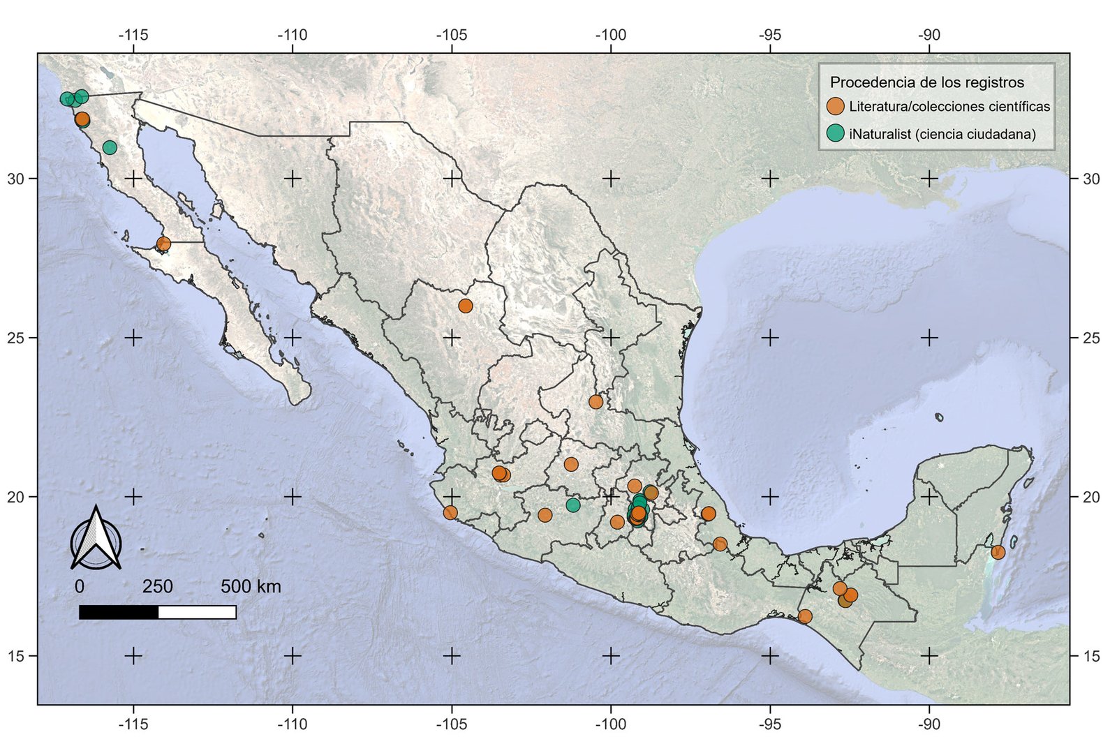
Tras el proceso de filtrado y validación, el número total de registros para L. humile en México fue de 100, de los cuales 30 corresponden a ejemplares preservados en colecciones científicas, 5 a registros documentados en la literatura y 65 a observaciones de categoría A provenientes de la plataforma de ciencia ciudadana iNaturalist. La extensión geográfica que abarcan los registros fue entre 32.57º y 16.23º de latitud norte y -117.08º y -87.84º de longitud este (fig. 2). La figura S1 del material suplementario 1 muestra el mapa de registros pertenecientes a la categoría B entendidos como indicios de la presencia de la especie.
Figura 2. Mapa de los registros históricos de Linepithema humile en México. Los puntos naranjas indican registros procedentes de la literatura y colecciones científicas mientras que los puntos verdes indican observaciones procedentes de la plataforma de ciencia ciudadana iNaturalist.
Análisis areográfico y reconstrucción temporal de la invasión
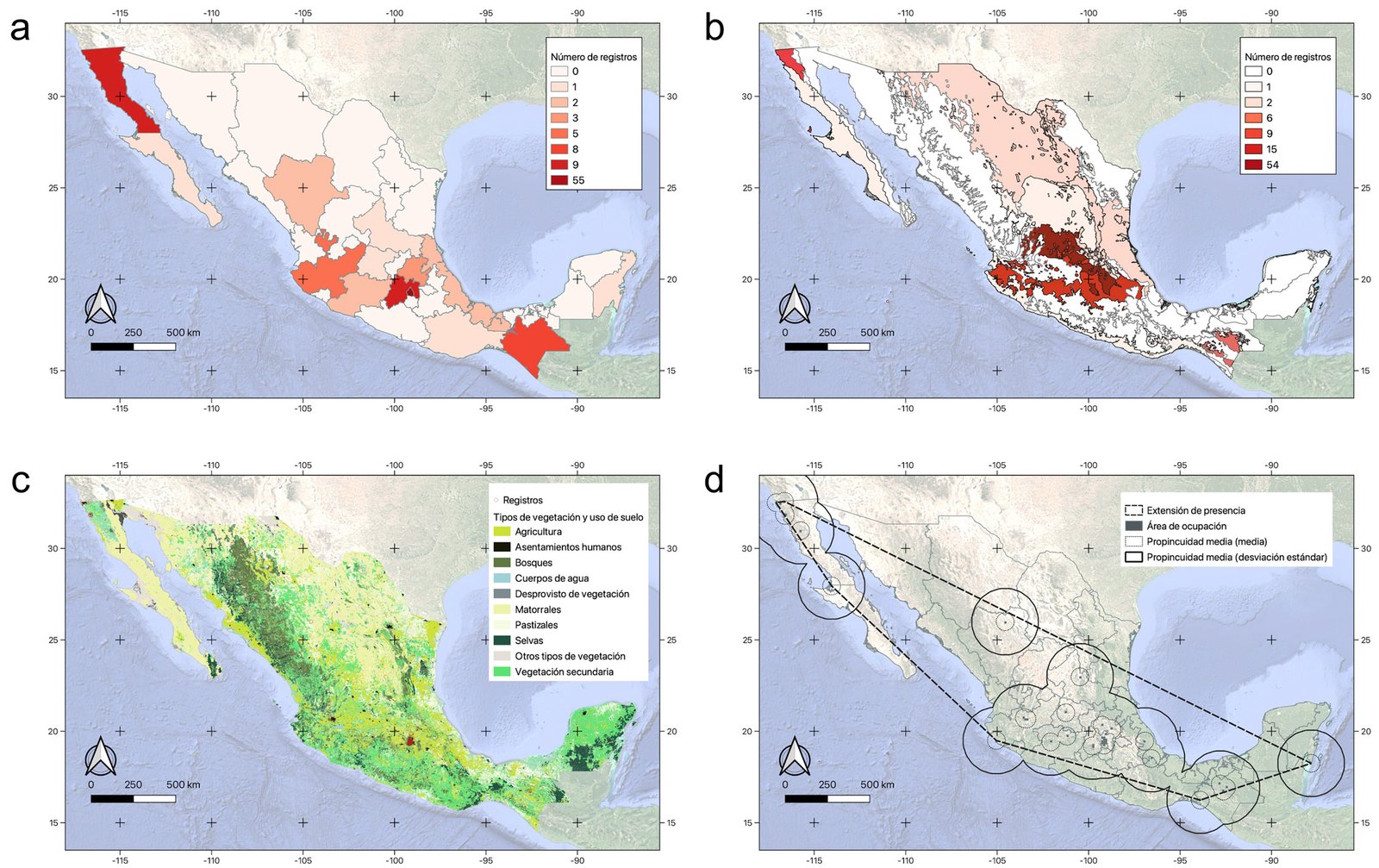
De acuerdo con los datos obtenidos y los diferentes métodos de inferencia de áreas de distribución, se obtuvo que L. humile se distribuye en 14 de los 32 estados de México (fig. 3a). La mayor concentración de registros se localiza en la Ciudad de México (anteriormente Distrito Federal, con 55 registros), seguida de Baja California (9) y el Estado de México (9). Los restantes estados presentan 8 o menos registros. En cuanto a las ecorregiones, L. humile se distribuye en 15 de ellas (fig. 3b), siendo el matorral del centro de México el que concentra el mayor número de registros (54), seguido de los bosques de pino-encino de la Faja Volcánica Transmexicana (14) y de salvia y chaparral costero de California (9). Finalmente, para los tipos de vegetación y uso de suelo, se encontraron registros en 15 categorías, 4 de ellas correspondientes a agricultura de temporal o riego, y una de vegetación secundaria, destacando, además, la presencia en áreas de asentamientos humanos (fig. 3c). La mayor cantidad de registros se obtuvo precisamente en zonas urbanas (74 registros), seguidas por áreas de agricultura de temporal anual (5 registros) y 4 categorías con 3 registros cada una: agricultura de riego anual y semipermanente, agricultura de temporal permanente, bosque cultivado y matorral desértico micrófilo.
Figura 3. Análisis areográfico de los registros de Linepithema humile en México: a) estados geopolíticos; b) ecorregiones (Olson et al., 2001); c) tipos de vegetación y uso de suelo de México (INEGI, 2023); d) distribución geográfica de L. humile en México inferida con 3 métodos: extensión de presencia (línea discontinua), área de ocupación (cuadros grises) y propincuidad media con el valor de la media (línea punteada) y la desviación estándar (línea negra continua).
El área de distribución geográfica obtenida mediante las 3 metodologías empleadas es congruente entre sí (fig. 3d). No obstante, los métodos de área de ocupación y propincuidad media utilizando el valor de la media podrían estar subestimando el área de distribución real de la especie. Por su parte, la extensión de presencia y propincuidad media con desviación estándar predicen que L. humile podría estar presente en prácticamente todos los estados del país, con excepción de Yucatán.
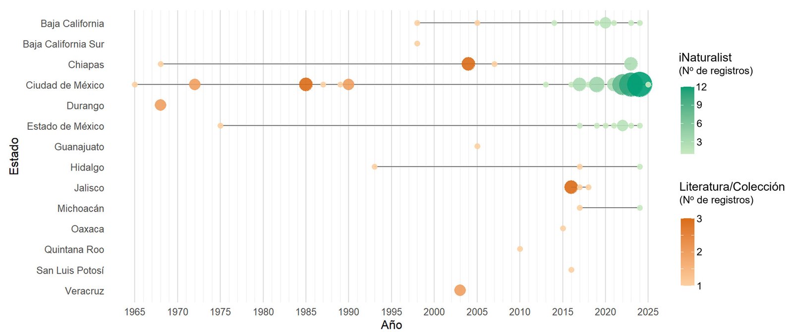
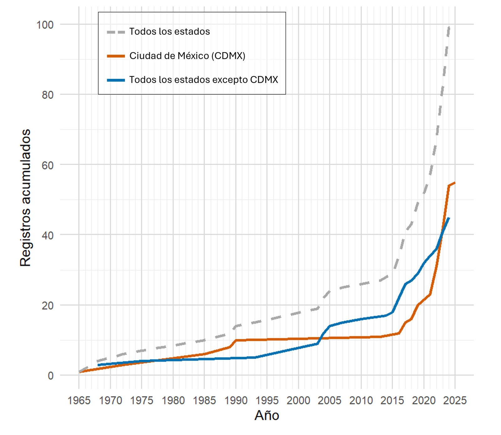
El registro confirmado más antiguo de la presencia de L. humile en México data de 1965, mientras que el más reciente, considerado en este estudio como presencia válida (categoría A), corresponde a abril de 2025 (figs. 3, 4) y como indicio a noviembre de 2025 (categoría B). La distribución temporal de los registros no es continua, se destaca la década de 1975 a 1985 como el intervalo más prolongado sin registros. Hasta 2015, la acumulación de registros fue gradual, sin superar las 3 citas anuales (fig. 4). A partir de 2016 se observa un incremento progresivo en el número de registros a nivel nacional (fig. 5). Este aumento es especialmente notable en la Ciudad de México, aunque en otros estados, como Baja California y el Estado de México, también experimentan este fenómeno (fig. 4). Los años con mayor cantidad de registros fueron 2022 (16 registros), 2023 (38) y 2024 (24), mostrando una tendencia creciente en el tiempo. Los datos procedentes de literatura y colecciones científicas aportan las primeras citas (4 y 10 respectivamente) para todos los estados donde se ha detectado la presencia de L. humile (material suplementario 1: tabla S1). Por su parte, los datos procedentes de iNaturalist, si bien no aportan nuevos registros a nivel de estado, confirman su presencia en la última década en 6 de ellos (fig. 4). El análisis espacial de la invasión, representado en el video, evidencia los periodos en los que no se registran observaciones y la acumulación progresiva de registros en la Ciudad de México, así como hallazgos esporádicos en otros estados (video: https://youtu.be/0yXOEUlDXD8).
Figura 4. Evolución temporal del número de registros de Linepithema humile para cada estado de México. En color naranja se representan los registros provenientes de literatura y/o colecciones científicas y en color verde los provenientes de plataformas de ciencia ciudadana (iNaturalist). El tamaño de los círculos y la intensidad de color son proporcionales al número de citas por año.Figura 5. Evolución temporal de los registros acumulados de Linepithema humile para la Ciudad de México (línea naranja), el resto de los estados (línea azul) y el conjunto de estados (línea gris discontinua).
Análisis del sesgo de urbanización y procedencia de los datos
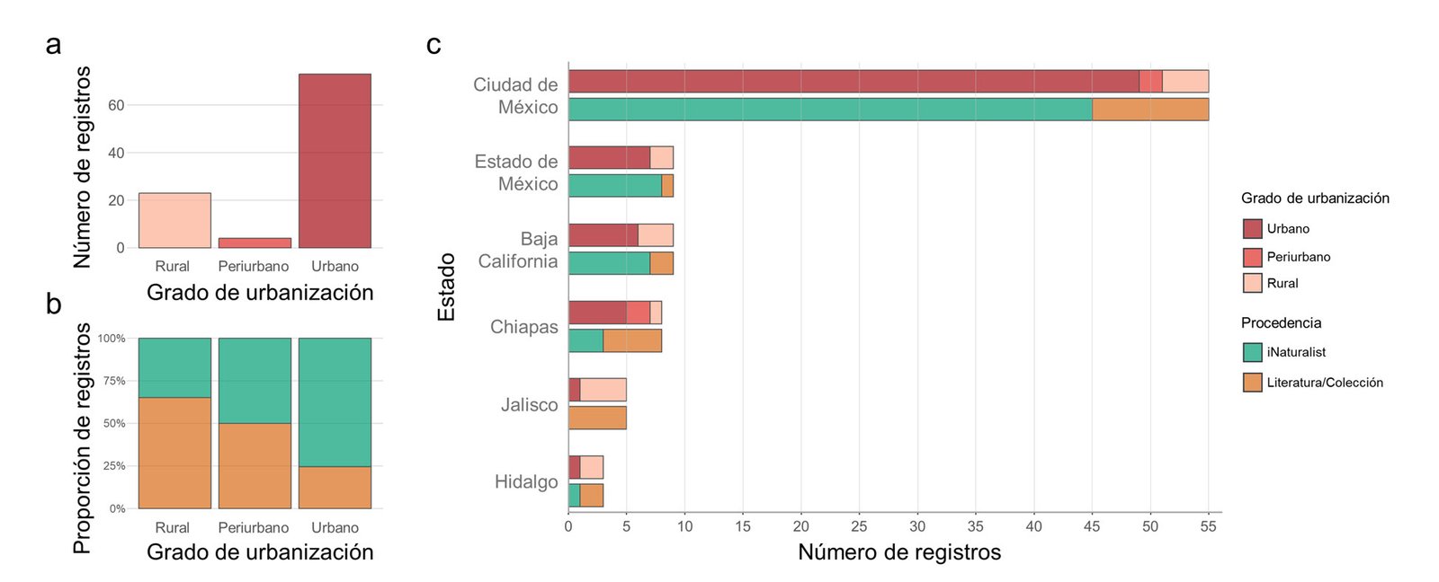
El número de registros mostró diferencias claras entre las categorías de población, con una mayor concentración de observaciones en entornos urbanos en comparación con zonas periurbanas y áreas rurales (fig. 6a). La proporción de observaciones provenientes de iNaturalist fue mayor en entornos urbanos mientras que los registros de literatura y colecciones científicas predominan en entornos rurales (fig. 6b). Los datos revelaron que la Ciudad de México concentra un número de registros urbanos muy grande dominados mayoritariamente por observaciones procedentes de iNaturalist. Esta situación, aunque con un número de registros mucho menor, también se da en los estados de México y Baja California, en contraste con otros estados del país, donde la contribución relativa de literatura y colecciones es mayor (fig. 6c).
Figura 6. a) Proporción de registros de Linepithema humile en México atendiendo a la procedencia (literatura y/o colecciones científicas y la plataforma de ciencia ciudadana iNaturalist) según el grado de urbanización (rural: < 250 habitantes/km²); periurbano: > 250 habs./km²; urbano: ≥ 1,000 habs./km²); b) número de registros por estado (se muestran los 6 estados con más registros) atendiendo al grado de urbanización (barra superior) y la procedencia de los datos (barra inferior).
La prueba χ² de Pearson reveló una asociación significativa entre la categoría de población y la procedencia de los datos (χ² = 13.06, gl = 2, p = 0.0015), indicando que la distribución de las fuentes no es independiente del grado de urbanización. Los modelos binomiales confirmaron este patrón (tabla 2). En el modelo sin covariables temporales (modelo A), los registros procedentes de entornos urbanos mostraron una probabilidad significativamente mayor de corresponder a iNaturalist en comparación con los entornos rurales. Al incorporar el año de registro como covariable (modelo B), el efecto de la categoría urbana se mantuvo significativo, mientras que el efecto del año fue positivo y estadísticamente significativo, reflejando un incremento progresivo en la contribución relativa de iNaturalist a lo largo del tiempo. Este modelo presentó una mejora sustancial del ajuste (reducción marcada de la desvianza residual y del AIC), lo que sugiere que el sesgo urbano está parcialmente mediado por un fuerte componente temporal asociado al incremento en la última década del uso de plataformas de ciencia ciudadana. El análisis de sensibilidad tras excluir los registros de Ciudad de México (modelo C) mostró que el efecto temporal mantenía su significación, mientras que el efecto de la urbanización se atenuaba y dejaba de ser estadísticamente significativo, lo que señala el gran peso que tienen los datos de la capital.
Predictor
Modelo A: sin covariables
Modelo B: covariable temporal (año)
Modelo C: sensibilidad
Intercepto
-0.63 ± 0.44
-4.77 ± 1.74**
-6.18 ± 2.63
Periurbano
0.63 ± 1.09
4.89 ± 14.38
-3.66 ± 4,612.21
Urbano
1.75 ± 0.52***
3.47 ± 1.32**
2.53 ± 1.57
Año
—
0.77 ± 0.24**
0.99 ± 0.40*
Nº observaciones
100
100
45
Residuo de desviación
116.81
21.63
13.63
AIC
122.81
29.63
21.63
Tabla 2. Modelos lineales generalizados binomiales que evalúan el efecto del nivel de urbanización y el tiempo (años) sobre la probabilidad de que los registros de Linepithema humile provengan de datos de ciencia ciudadana (iNaturalist) en lugar de la literatura o colecciones biológicas. Los coeficientes (β) se muestran en la escala logit ± error estándar. Se utilizaron entornos rurales (< 250 habitantes/km²) como categoría de referencia (periurbanos > 250 habs./km²; urbanos ≥ 1,000 habs./km²). El modelo de sensibilidad excluye los registros de Ciudad de México del modelo B. Niveles de significación: p < 0.05 (*), p < 0.01 (**), p < 0.001 (***).
Áreas de distribución potencial y papel de la urbanización
De acuerdo con el modelo consenso, la distribución potencial de L. humile en México se explica por las siguientes 5 variables: Bio7 – rango anual de temperatura, Bio5 – temperatura máxima del mes más cálido, Bio19 – precipitación del trimestre más frío, Bio15 – estacionalidad de las precipitaciones y densidad de población (proxy de urbanización). La contribución de las variables a los modelos se muestra en el material suplementario 1: tablas S2, S3). La evaluación del modelo consenso obtuvo buenos resultados con una calibración de AUC > 0.993, TSS > 0.913 y Kappa > 99.97 (material suplementario 1: tabla S4).
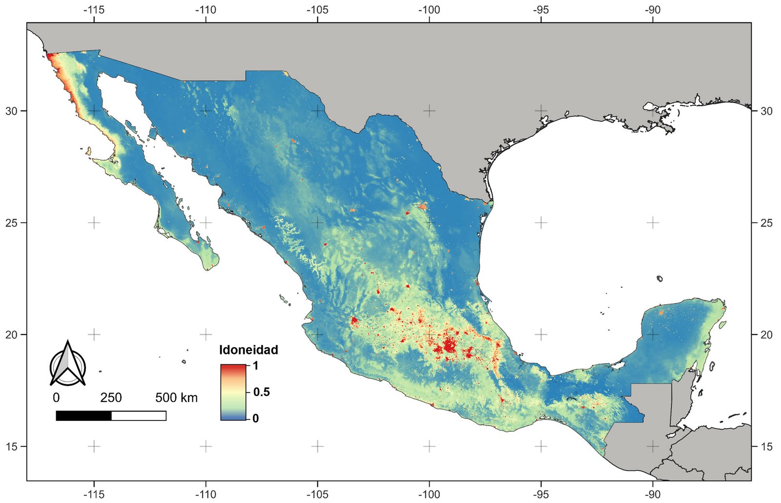
Los modelos denotan un alto grado de idoneidad en zonas altamente urbanizadas en torno al centro del país (fig. 7, idoneidad > 0.7) como por ejemplo en la Ciudad de México, Toluca, Puebla, Xalapa, Pachuca, Querétaro, Guanajuato, León o Aguascalientes, acompañadas de zonas de menor idoneidad en áreas naturales circundantes (idoneidad en torno a 0.5). En términos biogeográficos corresponden a localizaciones hacía el sur de la Sierra Madre Occidental y del desierto Chihuahuense junto con la Faja Volcánica Transmexicana, parte de la Sierra Madre del Sur y territorios en las Tierras Altas de Chiapas. El estado de Baja California, a lo largo de toda su costa oeste, también presenta valores de idoneidad altos. El resto del país presenta valores de idoneidad bajos, incluso en zonas costeras, con excepción de los núcleos urbanos repartidos por todo el territorio nacional. En el norte del país destaca la alta idoneidad en ciudades como Monterrey, Torreón, Chihuahua o Ciudad Juárez, aunque también hay zonas naturales de menor idoneidad que se extienden por la Sierra Madre Occidental y el norte de Chihuahua. En los modelos, los territorios que rodean el golfo de México, coincidiendo con Tamaulipas, las áreas costeras de Veracruz, Tabasco y la península de Yucatán obtienen valores de idoneidad muy bajos o nulos. Los resultados apoyan la idea de que la urbanización desempeña un papel importante en el patrón de distribución observado de L. humile.
Figura 7. Mapa de la distribución potencial de Linepithema humile atendiendo a variables climáticas y densidad de población en los límites geopolíticos de México.
Grado de expansión en la Ciudad de México
El número total de registros de L. humile en la Ciudad de México (hasta noviembre de 2025) asciende a 84, correspondientes a 121 observaciones antes de aplicar el filtro de autocorrelación espacial. De estos, 10 registros proceden de fuentes bibliográficas y de colecciones científicas, mientras que 74 corresponden a observaciones de iNaturalist, de las cuales 45 se consideran presencias válidas y 29 indicios. En consecuencia, se dispone de un total de 55 puntos de presencia válidos de L. humile en la Ciudad de México.
A efectos de los análisis biogeográficos realizados en este estudio, se excluyeron 112 de los 192 registros procedentes de iNaturalist, lo que representa 58.3% del total de datos aportados por esta plataforma a través de GBIF. Tras la superposición de una malla de cuadros de 1 × 1 km, se identificaron 47 cuadros con presencias válidas y 23 cuadros que representan indicios de la presencia de la especie (fig. 8), lo que supone 4.34% de cuadros (de un total de 1,612) con presencia confirmada o posible por parte de L. humile en CDMX.
Linepithema humile tiene presencia en 13 de las 16 alcaldías que componen la división administrativa de la Ciudad de México. Las alcaldías con mayor número de cuadros con presencias válidas se sitúan hacía el núcleo urbano: Coyoacán (10), Cuauhtémoc (5), Benito Juárez (4) y Miguel Hidalgo (4). Si bien L. humile se expande principalmente por las áreas urbanizadas, cabe destacar la presencia de la especie en zonas naturales o parques urbanos como es el caso de los Viveros de Coyoacán y en el entorno de la Ciudad Universitaria, por su cercanía a la Reserva Ecológica del Pedregal de San Ángel (fig. 8). Asimismo, existen indicios de su presencia cerca de El Tepeyac, al norte de la ciudad y hacia el sur, en las zonas de conservación ecológica de los ejidos de Xochimilco y San Gregorio Atlapulco, La Loma y la zona ecológica y cultural del bosque de Tlalpan.
Asignación de supercolonias
En total se recolectaron 14 muestras correspondientes a 11 de las 16 alcaldías que conforman la ciudad (tabla S5), con distancias entre puntos de muestreo que variaron entre 1.6 km y 23.8 km. Se realizaron 175 ensayos de comportamiento, en los cuales todos los cruces resultaron en interacción amistosa (en ningún caso se dio una señal de enfrentamiento) entre los pares de individuos (tabla S6), lo que indica la presencia de una única supercolonia en la Ciudad de México con base en las pruebas realizadas con las muestras recolectadas.
Discusión
La distribución de L. humile en México no muestra una continuidad geográfica clara, sino un patrón espacialmente fragmentado a lo largo de gran parte del territorio nacional. Además, el patrón es temporalmente discontinuo durante los aproximadamente 60 años desde sus primeros registros en el país. Este patrón es consistente con el observado en numerosas especies sinantrópicas a escala global, caracterizadas por distribuciones amplias fuera de sus áreas nativas y por una fuerte asociación con actividades humanas (Faeth et al., 2011). En este contexto, las hormigas destacan como uno de los grupos animales con mayor número de especies globalmente distribuidas, estrechamente ligadas al ser humano y capaces de colonizar tanto ambientes antrópicos como entornos naturalizados fuera de su distribución geográfica nativa (Bertelsmeier, 2021; Carpintero et al., 2014; Menke et al., 2011; Vonshak y Gordon, 2015).
A pesar de la afinidad generalmente descrita de L. humile por territorios costeros en regiones invadidas a escala global (Hartley et al., 2006; Roura-Pascual et al., 2004, 2011), en México su distribución se concentra principalmente en áreas del interior del país, con una clara asociación con entornos urbanizados. Los modelos de distribución potencial indican una alta idoneidad climática en regiones centrales, en concordancia con lo propuesto por algunos autores (Hartley et al., 2006; Jung et al., 2022; Li et al., 2024), mientras que la mayor parte del litoral mexicano —con la excepción de algunos núcleos urbanos y la costa noroeste de la península de Baja California— presenta una idoneidad ambiental baja, en contraste con patrones descritos previamente (Roura-Pascual et al., 2004). Este patrón sugiere que la presencia de L. humile en México está fuertemente condicionada por la disponibilidad de ambientes antropizados que proporcionan condiciones favorables para su establecimiento, como áreas urbanas con espacios verdes o zonas agrícolas irrigadas, incluso en regiones que, desde un punto de vista climático, podrían resultar limitantes para su supervivencia.
Las vías de introducción de L. humile en México no están claramente identificadas (Rosas-Mejía y Janda, 2017). No obstante, el registro histórico más antiguo datado en 1965 en la Ciudad de México (leg. N.L.H. Krauss; Wetterer et al., 2009), junto con el papel central de esta urbe como nodo de comercio nacional e internacional, sugiere que la especie pudo haber sido introducida accidentalmente a través del transporte de mercancías procedentes de otras regiones del continente americano o de áreas previamente invadidas. De hecho, la distribución histórica previa a la década de 1990 muestra una concentración de registros en la Ciudad de México y las observaciones posteriores, sin considerar los registros de la península de Baja California, se han ido sucediendo en estados adyacentes o muy próximos a la capital del país, llegando a territorios más alejados en las últimas décadas como Chiapas, Quintana Roo o Jalisco.
Sin embargo, no puede descartarse la existencia de introducciones independientes no documentadas en otras regiones del país producidas con anterioridad. En concreto, Baja California constituye actualmente una de las entidades con mayor número de registros, concentrados principalmente en la ciudad de Tijuana y sus alrededores. Considerando la amplia presencia de L. humile en la vecina ciudad de San Diego (EUA) y que la primera cita confirmada para el estado de California data de 1905 (Smith, 1936; Wetterer et al., 2009), resulta plausible que una de las vías de entrada de la especie en México haya sido a través de la frontera con California.
No obstante, la interpretación de los patrones espaciales y temporales descritos debe considerarse a la luz de las limitaciones inherentes a las fuentes de datos disponibles. La distribución fragmentada y la aparente expansión reciente de L. humile en México pueden estar condicionadas, al menos en parte, por diferencias en el esfuerzo de muestreo, la accesibilidad a determinadas regiones y un marcado sesgo espacial hacia entornos urbanos, donde la probabilidad de detección y reporte es mayor. Asimismo, el incremento de registros en las últimas décadas coincide con la consolidación de plataformas de ciencia ciudadana, como iNaturalist, lo que puede amplificar tendencias temporales que no necesariamente reflejan cambios reales en la distribución de la especie. Adicionalmente, la fiabilidad taxonómica de los registros procedentes de estas plataformas depende de procesos de validación rigurosos, especialmente en grupos con especies morfológicamente similares y de tamaño pequeño. En conjunto, estos aspectos ponen de manifiesto la necesidad de evaluar críticamente el papel de las distintas fuentes de información empleadas y justifican un análisis específico de los sesgos y limitaciones asociados al uso de datos de ciencia ciudadana en el seguimiento de L. humile en México.
Papel de la ciencia ciudadana en el seguimiento de Linepithema humile en México: sesgos y limitaciones
En los últimos años, las plataformas de ciencia ciudadana han adquirido un papel cada vez más relevante en el estudio de la distribución y dinámica espacial de especies, especialmente en contextos donde los datos procedentes de muestreos sistemáticos son escasos o desigualmente distribuidos (Chandler et al., 2017). En el caso de L. humile en México, la incorporación de registros procedentes de iNaturalist a escala regional ha permitido ampliar de forma significativa la cobertura temporal de la información disponible; sin embargo, su contribución ha sido más limitada desde el punto de vista espacial. Por ejemplo, no ha detectado nuevas citas a nivel de estado, aunque aporta indicios de su presencia en el estado de Aguascalientes.
A escala local, la aportación de iNaturalist resulta más relevante, al haber advertido la presencia de la especie en localidades concretas previamente no documentadas en la literatura o en colecciones científicas, como Tecate y San Quintín en Baja California, o varias localidades del Estado de México (p. ej., Zumpango de Ocampo, Santa María Cuevas, Bosques de Ixtacala y Tultepec), así como indicios en Toluca de Lerdo y áreas circundantes. No obstante, es en la Ciudad de México donde la contribución de iNaturalist resulta más evidente, al revelar la presencia de L. humile en una proporción considerable de su extensión urbana.
No obstante, el uso de este tipo de datos con fines biogeográficos conlleva limitaciones inherentes, relacionadas tanto con sesgos de muestreo —como la sobrerrepresentación de entornos urbanos y accesibles— como con la variabilidad en la calidad taxonómica de las observaciones. Estas limitaciones hacen necesario un análisis crítico de la información generada por plataformas participativas y la aplicación de criterios de validación específicos, particularmente en especies invasoras con implicaciones ecológicas y de gestión relevantes. En el caso de L. humile, los errores de identificación pueden derivarse de la variabilidad en la calidad de las imágenes, de la ausencia de caracteres diagnósticos clave visibles o de la confusión con especies ecológica y morfológicamente afines —por ejemplo, dentro de la subfamilia Dolichoderinae, géneros como Azteca, Dorymyrmex o Tapinoma Foerster, 1850—, lo que limita el uso directo de estos registros con fines biogeográficos sin la aplicación de procesos adicionales de validación taxonómica.
En este contexto, el sistema de validación aplicado en el presente estudio responde a la necesidad de asegurar la fiabilidad taxonómica y espacial de los registros procedentes de iNaturalist, manteniendo al mismo tiempo su valor informativo para el análisis biogeográfico. La clasificación de las observaciones en categorías A, B y C, basada en la visibilidad de caracteres morfológicos diagnósticos, el grado de consenso experto y la coherencia espacial entre registros próximos, permitió discriminar entre presencias confirmadas, indicios plausibles y observaciones poco confiables para análisis espaciales. En conjunto, la estrategia adoptada proporciona un marco metodológico replicable que integra el potencial de la ciencia ciudadana con criterios de calidad acordes con estudios biogeográficos y de seguimiento de especies invasoras (Dimson et al., 2023; Johnson et al., 2020); esto limita el sesgo de muestreo y la sobrerrepresentación de registros asociados a variables antrópicas como la densidad de población (Mair y Ruete, 2016).
Los resultados evidencian un marcado sesgo espacial en los registros de L. humile en México procedentes de iNaturalist hacia entornos urbanos, mientras que los registros de literatura y colecciones científicas adquieren más relevancia en áreas rurales. Este patrón no puede atribuirse exclusivamente a un artefacto metodológico: aunque la concentración de observadores en grandes áreas metropolitanas introduce un sesgo de muestreo evidente, la elevada densidad de registros en la Ciudad de México también sugiere una realidad biológica, coherente con la alta idoneidad de los entornos urbanos para la expansión de esta especie invasora asociada a ambientes antropizados.
El efecto temporal detectado en los modelos estadísticos sugiere que el sesgo urbano se ha intensificado en años recientes, en paralelo al crecimiento de la ciencia ciudadana. Este resultado refuerza la necesidad de considerar explícitamente el año de registro en análisis basados en datos de presencia, especialmente cuando se combinan fuentes heterogéneas. El análisis de sensibilidad tras excluir la Ciudad de México indica que, si bien el sesgo temporal es generalizado, la intensidad del patrón urbano se concentra espacialmente, lo que sugiere que las grandes áreas metropolitanas actúan como amplificadores tanto del esfuerzo de muestreo como de la señal ecológica subyacente.
Importancia de la urbanización: el ejemplo de la Ciudad de México
La distribución actual de L. humile en México puede interpretarse como el resultado de una marcada afinidad por los entornos urbanos, entendida tanto como una preferencia ecológica como por un comportamiento adaptativo frente a ambientes fuertemente antropizados (Borden y Flory, 2021; López-Collar et al., 2024).
Los resultados de los modelos de idoneidad respaldan la hipótesis de que la afinidad de L. humile por entornos urbanos constituye un factor clave en su dispersión en México (Roura-Pascual et al., 2009). El papel de las ciudades como “islas climáticas”, documentado tanto para L. humile en otras regiones invadidas como para otras especies sinantrópicas (López-Collar et al., 2024; Polidori et al., 2021), resulta coherente con la fragmentación espacial y la marcada asociación urbana observadas en el país. En este contexto, las áreas urbanas pueden funcionar como refugios bioclimáticos en regiones donde las condiciones ambientales generales serían limitantes, favoreciendo la persistencia local de la especie a modo de reservorios y actuando como focos de dispersión a escalas espaciales más amplias.
Además, la prevalencia de L. humile en zonas urbanas se alinea con un patrón común entre especies no nativas en México, cuyos registros son más frecuentes en contextos urbanos (Rosas-Mejía et al., 2021). Las áreas verdes, parques y jardines botánicos ubicados en ciudades proporcionan microhábitats que permiten condiciones ideales de humedad, recursos alimenticios y refugio, favoreciendo la formación de nuevas colonias de la hormiga argentina (Hartley y Lester, 2003; López-Collar y Cabrero-Sañudo, 2021; Suarez et al., 2001). El comercio y translocación de plantas ornamentales y materiales de jardinería entre viveros, otros espacios verdes urbanos y hogares, puede desempeñar un papel importante en la propagación e introducción accidental de estas colonias en nuevas áreas a través de ciudades y puertos (Obregón y Reyes-López, 2016; Rosas-Mejía et al., 2021; Ward et al., 2005).
En este marco, la Ciudad de México —la segunda entidad federativa más poblada del país, con más de 9.2 millones de habitantes (INEGI, 2020b)— reúne de manera excepcional estos factores, configurándose como un entorno altamente favorable para la expansión de L. humile. Las colonias de esta hormiga ocupan amplias extensiones en parques y áreas verdes urbanas y se observan con frecuencia formando largas hileras en calles arboladas y zonas residenciales adyacentes a jardines privados (López-Collar, D., obs. pers.). La coexistencia de otras especies exóticas o invasoras, como Tapinoma melanocephalum (Fabricius, 1793) y Paratrechina longicornis (Latreille, 1802), sugiere además un escenario de fuerte presión sobre las comunidades de hormigas nativas, potencialmente asociado a procesos de desplazamiento y homogenización biótica (Vázquez-Franco, C. M., obs. pers.).
Finalmente, los ensayos de agresividad realizados indican la posible presencia de una única supercolonia de L. humile en la Ciudad de México, lo que implica la ocupación de cientos de km² por un mismo sistema cooperativo. Este patrón ha sido documentado en otras regiones invadidas, como Australia, donde Suhr et al. (2009) describen una supercolonia ampliamente extendida en la ciudad de Melbourne y genéticamente similar a colonias de otras ciudades, lo que apunta a la existencia de una estructura supercolonial a escala continental. Las consecuencias ecológicas de estas estructuras supercoloniales, aún poco estudiadas en entornos urbanos, podrían ser particularmente graves para la diversidad de hormigas nativas y para el funcionamiento de los ecosistemas urbanos en México. Si bien las colonias de la Ciudad de México no han podido asignarse a ningún linaje previamente descrito —debido a la ausencia de análisis comparativos con poblaciones de otras regiones, así como de estudios de hidrocarburos cuticulares o marcadores genéticos (Blight et al., 2017; Vogel et al., 2010)—, el presente trabajo constituye un punto de partida para futuras investigaciones orientadas a analizar la dinámica de supercolonias en México y su integración en un contexto global, lo que permitiría avanzar en la reconstrucción del proceso de invasión de la especie.
La combinación de fuentes de información heterogéneas —literatura científica, colecciones biológicas y plataformas de ciencia ciudadana— ha resultado esencial para reconstruir la dinámica espacial y temporal de la invasión de L. humile en México. Sin embargo, ha puesto de relieve la necesidad de aplicar protocolos rigurosos de validación taxonómica y de abordar explícitamente los sesgos espaciales y temporales asociados a los datos procedentes de iNaturalist. La presencia de L. humile en México no responde a un patrón de expansión continua producido únicamente por la idoneidad climática regional, sino a un proceso espacialmente fragmentado y estrechamente vinculado a la urbanización. Los entornos urbanos actúan como núcleos de establecimiento, persistencia y dispersión secundaria, funcionando como “islas bioclimáticas” que mitigan las restricciones ambientales a escala regional y favorecen la consolidación de poblaciones viables. Especialmente en la Ciudad de México, la amplia expansión detectada, junto con la evidencia preliminar de una única supercolonia, sugiere un elevado grado de integración poblacional, con potenciales consecuencias significativas para la estructura de las comunidades de hormigas nativas y para los procesos ecológicos en este entorno urbano. En conjunto, los resultados de esta investigación destacan la importancia de enfoques que integren muestreos sistemáticos y herramientas participativas sometidas a procesos rigurosos de validación taxonómica en análisis biogeográficos, y subrayan la necesidad de incorporar la dimensión urbana en las estrategias de monitoreo, prevención y gestión de L. humile y otras especies invasoras en México.
Agradecimientos
Diego Gabriel Rosas-Barrera, Frida Cecilia Sánchez-Rivera, Frida Itzel Madrid-Mier, Ana Mitzi Ramírez-Arellano, Omar Barrera-Moreno, Alina Katia Juárez-Medina y Gerardo Rodríguez-Tapia proporcionaron retroalimentación en versiones preliminares de este manuscrito. Agradecemos a Eduardo Martínez Alpízar y a Verónica Rincón Rubio por su asistencia en la recolección de muestras en la Ciudad de México. Extendemos los agradecimientos a todas las personas que han contribuido al conocimiento biogeográfico de Linepithema humile en México a través de la plataforma de ciencia ciudadana iNaturalist. Agradecemos extensamente la donación, por parte del Museo de Zoología Alfonso L. Herrera (UNAM) a la Colección de Entomología de la Universidad Complutense de Madrid, de los ejemplares de L. humile recolectados en Ciudad de México. Agradecemos a los revisores anónimos sus comentarios y sugerencias que mejoraron sustancialmente este trabajo.
Referencias
Álvarez-Blanco, P., Caut, S., Cerdá, X. y Angulo, E. (2017). Native predators living in invaded areas: responses of terrestrial amphibian species to an Argentine ant invasion. Oecologia, 185, 95–106. https://doi.org/10.1007/s00442-017-3929-x
Angulo, E., Guénard, B., Balzani, P., Bang, A., Frizzi, F., Masoni, A. et al. (2024). The Argentine ant, Linepithema humile: natural history, ecology and impact of a successful invader. Entomologia Generalis, 44, 41–61. https://dx.doi.org/10.1127/entomologia/2023/2187
Angulo, E., Hoffmann, B. D., Ballesteros-Mejia, L., Taheri, A., Balzani, P., Bang, A. et al. (2022). Economic costs of invasive alien ants worldwide. Biological Invasions, 24, 2041–2060. https://doi.org/10.1007/s10530-022-02791-w
AntWeb. (2024). Versión 8.112. California Academy of Sciences. Recuperado el 26 octubre, 2024 de: https://www.antweb.org
Bertelsmeier, C. (2021). Globalization and the anthropogenic spread of invasive social insects. Current Opinion in Insect Science, 46, 16–23. https://doi.org/10.1016/j.cois.2021.01.006
Blancafort, X. y Gómez, C. (2005). Consequences of the Argentine ant, Linepithema humile (Mayr), invasion on pollination of Euphorbia characias (L.) (Euphorbiaceae). Acta Oecologica, 28, 49–55. https://doi.org/10.1016/j.actao.2005.02.004
Blight, O., Berville, L., Vogel, V., Hefetz, A., Renucci, M., Orgeas, J. et al. (2012). Variation in the level of aggression, chemical and genetic distance among three supercolonies of the Argentine ant in Europe. Molecular Ecology, 21, 4106–4121. https://doi.org/10.1111/j.1365-294X.2012.05668.x
Blight, O., Josens, R., Bertelsmeier, C., Abril, S., Boulay, R. y Cerdá, X. (2017). Differences in behavioural traits among native and introduced colonies of an invasive ant. Biological Invasions, 19, 1389–1398. https://doi.org/10.1007/s10530-016-1353-5
Bolton, B. (2024). An online catalog of the ants of the World. California Academy of Sciences. Recuperado el 30 mayo, 2023 de: http://antcat.org
Borden, J. B. y Flory, S. L. (2021). Urban evolution of invasive species. Frontiers in Ecology and the Environment, 19, 184–191. https://doi.org/10.1002/fee.2295
Brandt, M., Van Wilgenburg, E. y Tsutsui, N. D. (2009). Global- scale analyses of chemical ecology and population genetics in the invasive Argentine ant. Molecular Ecology, 18, 997– 1005. https://doi.org/10.1111/j.1365-294X.2008.04056.x
Burgess, H. K., DeBey, L. B., Froehlich, H. E., Schmidt, N., Theobald, E. J., Ettinger, A. K. et al. (2017). The science of citizen science: exploring barriers to use as a primary research tool. Biological Conservation, 208, 113–120. https://doi.org/10.1016/j.biocon.2016.05.014
Carpintero, S., Retana, J., Cerdá, X., Reyes-López, J. y Arias de Reyna, L. (2014). Exploitative strategies of the invasive Argentine ant (Linepithema humile) and native ant species in a southern Spanish pine forest. Environmental Entomo- logy, 36, 1100–1111. https://doi.org/10.1093/ee/36.5.1100
Chandler, M., See, L., Copas, K., Bonde, A. M., López, B. C., Danielsen, F. et al. (2017). Contribution of citizen science towards international biodiversity monitoring. Biological Conservation, 213, 280–294. https://sedac.ciesin.columbia.Edu/data/collection/gpw-v3
Conabio (Comisión Nacional para el Conocimiento y Uso de la Biodiversidad). (2020). Áreas naturales protegidas estatales, municipales, ejidales, comunitarias y privadas de México 2020. Catálogo de metadatos geográficos. Comisión Nacional para el Conocimiento y Uso de la Biodiversidad. Recuperado el 16 marzo, 2026 de http://geoportal.conabio.gob.mx/metadatos/doc/html/anpest20gw.html
Dáttilo, W., Vásquez-Bolaños, M., Ahuatzin, D. A., Antoniazzi, R., Chávez-González, E., Corro, E. et al. (2019) Mexico ants: incidence and abundance along the Nearctic-Neotropical interface. Ecology, 101, e02944. https://doi.org/10.1002/ecy.2944
Demetriou, J., Borowiec, L., Georgiadis, C., Economo, E. P., Roy, H. E., Martinou, A. F. et al. (2025). Citizen-science supplements species inventories and reveals the invasion of Monomorium exiguum and Pheidole parva (Hymenoptera: Formicidae) in Cyprus. Sociobiology, 72, e11594. https://doi.org/10.13102/sociobiology.v72i3.11594
Dimson, M., Berio-Fortini, L., Tingley, M. W. y Gillespie, T. W. (2023). Citizen science can complement professional invasive plant surveys and improve estimates of suitable habitat. Diversity and Distributions, 29, 1141–1156. https://doi.org/10.1111/ddi.13749
Faeth, S. H., Bang, C. y Saari, S. (2011). Urban biodiversity: patterns and mechanisms. Annals of the New York Academy of Sciences, 1223, 69–81. https://doi.org/10.1111/j.1749-6632.2010.05925.x
Fick, S. E. y Hijmans, R. J. (2017). WorldClim 2: new 1-km spatial resolution climate surfaces for global land areas. International Journal of Climatology, 37, 4302–4315. https://doi.org/10.1002/joc.5086
Geldmann, J., Heilmann-Clausen, J., Holm, T. E., Levinsky, I., Markussen, B. O., Olsen, K. et al. (2016). What determines spatial bias in citizen science? Exploring four recording schemes with different proficiency requirements. Diversity and Distributions, 22, 1139–1149. https://doi.org/10.1111/ddi.12477
Giraud, T., Pedersen, J. S. y Keller, L. (2002). Evolution of supercolonies: the Argentine ants of southern Europe. Proceedings of the National Academy of Sciences, 99, 6075–6079. https://doi.org/10.1073/pnas.092694199
Gómez, C. y Abril, S. (2008). Linepithema humile (Argentine ant). Centre for Agriculture and Biosciences International, CABI Compendium. Recuperado el 15 septiembre, 2024 de https://doi.org/10.1079/cabicompendium.30839
Gómez, C. y Oliveras, J. (2003). Can the Argentine ant (Linepithema humile, Mayr) replace native ants in myrmecochory? Acta Oecologica, 24, 47–53. https://doi.org/10.1016/S1146-609X(03)00042-0
Guénard, B., Weiser, M., Gomez, K., Narula, N. y Economo, E. P. (2017). The Global Ant Biodiversity Informatics (GABI) database: a synthesis of ant species geographic distributions. Myrmecological News, 24, 83–89. https://doi.org/10.25849/myrmecol.news_024:083
Guzmán, P., Bhowmik, S., Gaya, G., Cercós, J., Cabrero, F. J., Pino, J. et al. (2023). Informe anual uBMS 2023. Bellaterra: CREAF. Informe inédito.
Harris, R. J. (2002). Potential impact of the Argentine ant (Linepithema humile) in New Zeland and options for its control. En I. Mackenzie (Ed.), Science of conservation 196. Wellington: Department of Conservation.
Hartley, S. y Lester, P. J. (2003). Temperature-dependent development of the Argentine ant, Linepithema humile (Mayr) (Hymenoptera: Formicidae): a degree-day model with implications for range limits in New Zealand. New Zealand Entomologist, 26, 91–100. https://doi.org/10.1080/00779962.2003.9722113
Hartley, S., Harris, R. y Lester, P. J. (2006). Quantifying uncertainty in the potential distribution of an invasive species: climate and the Argentine ant. Ecology Letters, 9, 1068– 1079. https://doi.org/10.1111/j.1461-0248.2006.00954.x
Hiller, T. y Haelewaters, D. (2019). A case of silent invasion: citizen science confirms the presence of Harmonia axyridis (Coleoptera, Coccinellidae) in Central America. Plos One, 14, e0220082. https://doi.org/10.1371/journal.pone.0220082
Holway, D. A. y Suarez, A. V. (2006). Homogenization of ant communities in mediterranean California: the effects of urbanization and invasion. Biological Conservation, 127, 319–326. https://doi.org/10.1016/j.biocon.2005.05.016
Holway, D. A., Lach, L., Suarez, A. V., Tsutsui, N. D. y Case, T. J. (2002). The causes and consequences of ant invasions. Annual Review of Ecology and Systematics, 33, 181–233. https://doi.org/10.1146/annurev.ecolsys.33.010802.150444
INEGI (Instituto Nacional de Geografía, Estadística e Informática). (2019). Área geoestadística básica urbana, 2019. Catálogo de metadatos geográficos. Comisión Nacional para el Conocimiento y Uso de la Biodiversidad. Recuperado el 16 marzo, 2026 de: http://geoportal.conabio.gob.mx/metadatos/doc/html/agbumge19gw.html
INEGI (Instituto Nacional de Geografía, Estadística e Informática). (2020a). Áreas Geoestadísticas Municipales. Límites de las Alcaldías. Marco Geoestadístico. Recuperado el 20 febrero, 2024 de: https://www.inegi.org.mx/temas/mg/
INEGI (Instituto Nacional de Geografía, Estadística e Informática). (2023). Biblioteca digital de Mapas. Recuperado el 20 febrero, 2024 de: https://www.inegi.org.mx/app/mapas/
Janicki, J., Narula, N., Ziegler, M., Guénard, B. y Economo, E. P. (2016). Visualizing and interacting with large- volume biodiversity data using client-server web-mapping applications: the design and implementation of antmaps. org. Ecological Informatics, 32, 185–193. https://doi.org/10.1016/j.ecoinf.2016.02.006
Johnson, B. A., Mader, A. D., Dasgupta, R. y Kumar, P. (2020). Citizen science and invasive alien species: an analysis of citizen science initiatives using information and communications technology (ICT) to collect invasive alien species observations. Global Ecology and Conservation, 21, e00812. https://doi.org/10.1016/j.gecco.2019.e00812
Johnson, R. A. y Ward, P. S. (2002). Biogeography and endemism of ants (Hymenoptera: Formicidae) in Baja California, Mexico: afirst overview. Journal of Biogeography, 29, 1009– 1026. https://doi.org/10.1046/j.1365-2699.2002.00746.x
Jung, J. M., Kim, S. H., Jung, S. y Lee, W. H. (2022). Spatial and climatic analyses for predicting potential distribution of an invasive ant, Linepithema humile (Hymenoptera: Formicidae). Entomological Science, 25, e12527. https://doi.org/10.1111/ens.12527
Li, T., Jiang, P., Liu, J., Zhu, J., Zhao, S., Li, Z. et al. (2024). Considering climate change impact on the global potential geographical distribution of the invasive Argentine ant and little fire ant. Bulletin of Entomological Research, 114, 454–465. https://doi.org/10.1017/S0007485324000270
Lin, D., Foster, D. P. y Ungar, L. H. (2011). VIF regression: a fast regression algorithm for large data. Journal of the American Statistical Association, 106, 232–247. https://doi.org/10.1198/jasa.2011.tm10113
López-Collar, D. y Cabrero-Sañudo, F. J. (2021). Update on the invasion status of the Argentine ant, Linepithema humile (Mayr, 1868), in Madrid, a large city in the interior of the Iberian Peninsula. Journal of Hymenoptera Research, 85, 161–177. https://doi.org/10.3897/jhr.85.65725
López-Collar, D., Cabrero-Sañudo, F. J. y Gil-Tapetado, D. (2024). The urban island: climatic suitability of Linepithema humile (Hymenoptera: Formicidae) and the role of cities in the invasion of the Western Palearctic. Integrative Zoology, 20, 1169–1184. https://doi.org/10.1111/1749-4877.12903
Lucky, A., Savage, A. M., Nichols, L. M., Castracani, C., Shell, L., Grasso, D. A. et al. (2014). Ecologists, educators, and writers collaborate with the public to assess backyard diversity in The School of Ants Project. Ecosphere, 5, 78. http://dx.doi.org/10.1890/ES13-00364.1
Mair, L. y Ruete, A. (2016). Explaining spatial variation in the recording effort of citizen science data across multiple taxa. Plos One, 11, e0147796. https://doi.org/10.1371/journal.pone.0147796
Mason, B. M., Mesaglio, T., Heitmann, J. B., Chandler, M., Chowdhury, S., Gorta, S. B. Z. et al. (2025). iNaturalist accelerates biodiversity research. Bioscience, 75, 953–965. https://doi.org/10.1093/biosci/biaf104
Mateo, R. G., Morales-Barbero, J., Zarzo-Arias, A., Lima, H., Gómez-Rubio, V. y Goicolea, T. (2024). sabinaNSDM: an R package for spatially nested hierarchical species distribution modelling. Methods in Ecology & Evolution, 15, 1796–1803. https://doi.org/10.1111/2041-210X.14417
Mayr, G. (1868). Formicidae novae Americanae collectae a Prof. P. de Strobel. Annuario della Società dei Naturalisti e Matematici, Modena, 3,161–178.
Menke, S. B., Guénard, B., Sexton, J. O., Weiser, M. D., Dunn, R. R. y Silverman, J. (2011). Urban areas may serve as habitat and corridors for dry-adapted, heat tolerant species; an example from ants. Urban Ecosystems, 14, 135–163. https://doi.org/10.1007/s11252-010-0150-7
Menke, S. B., Ward, P. S. y Holway, D. A. (2018). Long- term record of Argentine ant invasions reveals enduring ecological impacts. Ecology, 99, 1194–1202. https://doi.org/10.1002/ecy.2200
Newell, W. y Barber T. C. (1913). The Argentine Ant. Washington DC: U.S. Department of Agriculture. Bureau of Entomo- logy Bulletin. https://doi.org/10.5962/bhl.title.109851
Obregón, R. y Reyes-López, J. (2016). Primera cita de la hormiga invasora Linepithema humile (Mayr, 1868) en el País Vasco (Hymenoptera, Formicidae). Revista Gaditana de Entomología, 7, 515–518.
Olson, D. M., Dinerstein, E., Wikramanayake, E. D., Burgess, N. D., Powell, G. V., Underwood, E. C. et al. (2001). Terrestrial ecoregions of the world: a new map of life on Earth: a new global map of terrestrial ecoregions provides an innovative tool for conserving biodiversity. Bioscience, 51, 933–938. https://doi.org/10.1641/0006-3568(2001)051[0933:TEOTWA]2.0.CO;2
Park, S. H., Hosoishi, S. y Ogata, K. (2014). Long-term impacts of Argentine ant invasion of urban parks in Hiroshima, Japan. Journal of Ecology and Environment, 37, 123–129. https://doi.org/10.5141/ecoenv.2014.015
Polidori, C., García-Gila, J., Blasco-Aróstegui, J. y Gil-Tapetado, D. (2021). Urban areas are favouring the spread of an alien mud-dauber wasp into climatically non-optimal latitudes. Acta Oecologica, 110, 103678. https://doi.org/10.1016/j.actao.2020.103678
Posit team. (2025). RStudio: integrated development environ- ment for R. Posit Software, PBC, Boston, MA. URL http://www.posit.co/
QGIS.org. (2025). QGIS Geographic Information System. QGIS Association. http://www.qgis.org
Queiroz, A. I. y Alves, D. (2018). People, transports and the spread of the Argentine ant in Europe, from c. 1850 to the present. CEM Cultura, Espaço y Memória, 7, 37–62.
Rapoport, E. H. (1975). Areografía: estrategias geográficas de las especies. Ciudad de México: Fondo de Cultura Económica.
Rendón-Salinas, E., Vieyra-Domínguez, R., Cruz-Piña, M., Mondragón-Contreras, G. Mendoza-Pérez M. y Martínez- Pacheco, A. (2026). Superficie forestal ocupada por las colonias de mariposas monarca en México durante la hibernación de 2025–2026. WWF México. https://www.correoreal.mx/
Rosas-Mejía, M. y Janda, M., (2017). Reporte final con la revisión de cuatro especies de hormigas con potencial invasor en México: Linepithema humile, Nylanderia fulva, Solenopsis invicta y Pheidole megacephala así como información de hormigas introducidas en el país. Proyecto GEF-Invasoras. Informe técnico. https://doi.org/10.13140/RG.2.2.21713.63841
Rosas-Mejía, M., Guénard, B., Aguilar-Méndez, M. J., Ghilardi, A., Vásquez-Bolaños, M., Economo, E. P. et al. (2021). Alien ants (Hymenoptera: Formicidae) in Mexico: the first database of records. Biological Invasions, 23, 1669–1680. https://doi.org/10.1007/s10530-020-02423-1
Roura-Pascual, N., Bas, J. M., Thuiller, W., Hui, C., Krug, R. M. y Brotons, L. (2009). From introduction to equilibrium: reconstructing the invasive pathways of the Argentine ant in a Mediterranean region. Global Change Biology, 15, 2101–2115. https://doi.org/10.1111/j.1365-2486.2009.01907.x
Roura-Pascual, N., Hui, C., Ikeda, T., Leday, G., Richardson, D. M., Carpintero, S. et al. (2011). Relative roles of climatic suitability and anthropogenic influence in determining the pattern of spread in a global invader. Proceedings of the National Academy of Sciences, 108, 220–225. https://doi.org/10.1073/pnas.1011723108
Roura-Pascual, N., Suarez, A. V., Gómez, C., Pons, P., Touyama, Y., Wild, A. L. et al. (2004). Geographical potential of Argentine ants (Linepithema humile Mayr) in the face of global climate change. Proceedings of the Royal Society of London. Series B: Biological Sciences, 271, 2527–2535. https://doi.org/10.1098/rspb.2004.2898
Smith, M. R. (1936). Distribution of the Argentine ant in the United States and suggestions for its control or eradication. United States Department of Agriculture Circular, 387, 1–39.
Stanley, M. C. y Ward, D. F. (2012). Impacts of Argentine ants on invertebrate communities with below-ground consequences. Biodiversity and Conservation, 21, 2653– 2669. https://doi.org/10.1007/s10531-012-0324-0
Stringer, L. D., Stephens, A. E., Suckling, D. M. y Charles, J. G. (2009). Ant dominance in urban areas. Urban Ecosystems, 12, 503–514. https://doi.org/10.1007/s11252-009-0100-4
Suarez, A. V., Holway, D. A. y Case, T. J. (2001). Patterns of spread in biological invasions dominated by long-distance jump dispersal: insights from Argentine ants. Proceedings of the National Academy of Sciences, 98, 1095–1100. https://doi.org/10.1073/pnas.98.3.1095
Suhr, E. L., McKechnie, S. W. y O’Dowd, D. J. (2009). Genetic and behavioural evidence for a city-wide supercolony of the invasive Argentine ant Linepithema humile (Mayr) (Hymenoptera: Formicidae) in southeastern Australia. Australian Journal of Entomology, 48, 79–83. https://doi.org/10.1111/j.1440-6055.2008.00688.x
Sunamura, E., Hatsumi, S., Karino, S., Nishisue, K., Terayama, M., Kitade, O. et al. (2009). Four mutually incompatible Argentine ant supercolonies in Japan: inferring invasion history of introduced Argentine ants from their social structure. Biological Invasions, 11, 2329–2339. https://doi.org/10.1007/s10530-008-9419-7
Suzuki, A., Seko, Y., Sakamoto, H., y Goka, K. (2025). Detection of honey bee pathogenic viruses in Argentine ants Linepithema humile (Hymenoptera: Formicidae) invading Japan. Applied Entomology and Zoology, 60, 1–7. https://doi.org/10.1007/s13355-025-00904-0
Touyama, Y., Ogata, K. y Sugiyama, T. (2003). The Argentine ant, Linepithema humile, in Japan: assessment of impact on species diversity of ant communities in urban environments. Entomological Science, 6, 57–62. https://doi.org/10.1046/j.1343-8786.2003.00008.x
Vavrek, M. J. (2011). Fossil: palaeoecological and palaeogeographical analysis tools. Palaeontologia Elec- tronica, 14, 1–16.
Vogel, V., Pedersen, J. S., Giraud, T., Krieger, M. J. y Keller, L. (2010). The worldwide expansion of the Argentine ant. Diversity and Distributions, 16, 170–186. https://doi.org/10.1111/j.1472-4642.2009.00630.x
Vonshak, M. y Gordon, D. M. (2015). Intermediate disturbance promotes invasive ant abundance. Biological Conservation, 186, 359–367. https://doi.org/10.1016/j.biocon.2015.03.024
Ward, D. F., Harris, R. J. y Stanley, M. C. (2005). Human- mediated range expansion of Argentine ants Linepithema humile (Hymenoptera: Formicidae) in New Zealand. Sociobiology, 45, 401–407.
Werenkraut, V., Lescano, M. N., Elizalde, L. y Pirk, G. I. (2025). Citizen science quickly reveals the Argentine ant Linepithema humile (Mayr, 1868) distribution in an invaded urban area and provides unexpected findings. Neotropical Entomology, 54, 133. https://doi.org/10.1007/s13744-025-01348-5
Wetterer, J. K., Wild, A. L., Suarez, A. V., Roura-Pascual, N. y Espadaler, X. (2009). Worldwide spread of the Argentine ant, Linepithema humile (Hymenoptera: Formicidae). Myrmecological News 12, 187–194.
Wild, A. L. (2007). Taxonomic revision of the ant genus Linepithema (Hymenoptera: Formicidae). Berkeley: University of California Publications in Entomology.
Zina, V., Branco, M. y Franco, J. C. (2020). Impact of the invasive argentine ant in citrus agroecosystems: effects on the diversity and frequency of native ant species foraging on tree canopy. Insects, 11, 785. https://doi.org/10.3390/insects11110785
Los peces asociados a arrecifes del Parque Nacional Revillagigedo (Pacífico mexicano): un inventario curado, comentado e ilustrado
D. Ross Robertson a, *, Benjamin Frable b, Benjamin C. Victor c, William Ludt d, Michelle R. Gaither e, Carlos J. Estape f, Allison Morgan-Estape f, Diane Pitassy g, Katriina L. Ilves h, Omar Domínguez-Domínguez i, Omar Valencia-Méndez j, Arturo Ayala-Bocos k, Edgar Adrián Acevedo-Álvarez i, María Gloria Solís-Guzmán i, A. Karim Awhida-Robinson i, Luis Fernando Martínez-García i, Ayla Gabriela Ramos-Mayoral i, María Elena Castillo-Victor i, Xavier Madrigal-Guridi i, Juan Esteban Martínez-Gómez l, Eloísa Torres-Hernández m, Lee Richter n, Sara Richter n, Andre Michael Goolishian-Hernández o, Serenity Mitchell o, Jeffrey D. Haines p, Alasdair G. Dunlap-Smith q, Ellen Place r, Carol Cox s, Robert Cox s, Fernando Duarte-Ramos t, Carlos Armando Sánchez-Ortiz t
a Smithsonian Tropical Research Institute, Naos Marine Laboratory, Ft Amador, Balboa, Republic of Panamá b University of California San Diego, Scripps Institution of Oceanography, Marine Vertebrate Collection, 9500 Gilman Drive, La Jolla, CA 92093-0244, USA c Ocean Science Foundation, 4051, Glenwood, CA 92604, USA d Natural History Museum of Los Angeles County, Department of Ichthyology, 900 Exposition Blvd., Los Angeles, CA 90007, USA e University of Central Florida, Genomics and Bioinformatics Cluster, Department of Biology, 4110 Libra Drive, Orlando, FL 32816, USA f 197 Gulfview Drive, 33036 Islamorada, FL, USA g Smithsonian Institution, National Museum of Natural History, Museum Support Center, 4210 Silver Hill Rd., Suitland, MD 20746, USA h Canadian Museum of Nature, Research & Collections, P.O. Box 3443, Sta. D, Ottawa, Ontario, K1P 6P4 Canada i Universidad Michoacana de San Nicolás de Hidalgo, Facultad de Biología, Laboratorio de Biología Acuática, Edificio R, Planta Baja, Ciudad Universitaria, 58030 Morelia, Michoacán, Mexico j Centro de Investigación Científica y de Educación Superior de Ensenada, Departamento de Ecología Marina, Carretera Ensenada – Tijuana No. 3918, Zona Playitas, 22860 Ensenada, Baja California, Mexico k Ecosistemas y Conservación, Proazul Terrestre A.C., Benito Juárez 665, Centro, 2300 La Paz, Baja California Sur, Mexico l Instituto de Ecología A.C., Red de Interacciones Multitróficas, Carretera antigua a Coatepec 351, Col. El Haya, 91073 Xalapa, Veracruz, Mexico m Universidad Nacional Autónoma de México, Instituto de Biología, Departamento de Zoología, Pabellón Nacional de la Biodiversidad, Colección Nacional de Peces, Tercer Circuito, Ciudad Universitaria, Coyoacán, 04510 Ciudad de México, Mexico n Fish Bay #1, 00830 St. John VI, USA o 5000 estate enighed, PMB 337, 00830 St. John USVI, USA p 2310 SE Maniton Terrace, 34952 Port St. Lucie, FL, USA q 50 Tug Mountain Road, Orange, 03741 New Hampshire, USA r 17117 NE 5th St. 98008 Bellevue, WA, USA s 202 Coral Dr, 32456 Port St. Joe, FL, 32456 USA t Universidad Autónoma de Baja California Sur, Departamento de Ciencias Marinas y Costeras, Carretera al Sur Km. 5.5, 23080 La Paz, Baja California Sur, Mexico
Accurate inventories of species living at isolated islands are essential for understanding the biogeographic and functional composition of insular faunas, habitat area vs. faunal-size relations and levels of endemism, as well as for purposes of conservation and management. Constructing such inventories involves new field research and rigorous winnowing of existing records that have errors in specimen identification and metadata or are unsubstantiable due to a lack of reliable source information. This paper provides a curated, photographically illustrated inventory of reef-associated fishes found at the 4 islands in the Revillagigedo National Park (RNP), 400 km southwest of Baja California. We assessed the quality of data about records relating to 364 species and added new data (specimens of 132 species and images of 182 species) that confirm species occurrences at each island in the park. The resultant inventory includes 234 accepted species occurrences, with 121 unaccepted occurrences (33.2% of the assessed species). Among the confirmed species, 166-189 (70.9-80.8%) evidently are park residents. New information indicates that the RNP fauna includes 23 named and probable species of endemics, representing 9.8% of the accepted species and 12.2-13.9% of the residents, highlighting the uniqueness of the RNP and its importance for conservation.
Los inventarios precisos de especies en islas aisladas son esenciales para comprender la composición biogeográfica y funcional de las faunas insulares, las relaciones área-fauna y los niveles de endemismo, además de ser fundamentales para la conservación y manejo. Su elaboración requiere nuevas investigaciones de campo, además de un riguroso cribado de registros existentes con errores de identificación o metadatos no verificables. Este artículo presenta un inventario ilustrado de los peces asociados con arrecifes del Parque Nacional Revillagigedo (PNR), ubicado a 400 km al suroeste de Baja California. Se evaluó la calidad de registros de 364 especies, incorporando datos nuevos (especímenes de 132 especies e imágenes de 182) que confirman presencias en cada una de las islas. El inventario resultante incluye 234 presencias aceptadas y 121 no aceptadas (33.2 % de las especies evaluadas). Dentro las confirmadas, entre 166 y 189 especies (70.9%-80.8%) son residentes del parque. La nueva información indica que la fauna del PNR incluye 23 especies endémicas nombradas y probables, representando 9.8% de las especies aceptadas y entre 12.2% y 13.9% de los residentes, lo que ilustra la singularidad ecológica del PNR y su importancia para la conservación marina.
Accuracy in faunal inventories for reef fishes and other reef organisms at isolated tropical islands is important for a variety of reasons. Species inventories often provide the only data used to assess the biogeographic relationships Dubic et al., 2023; Hobbs et al., 2012, 2014; Robertson & Allen, 1996; Robertson & Cramer, 2009), as well as many studies of their composition in terms of functional ecological characteristics (e.g., Bender et al., 2013; Dubuc et al., 2023; Ferrari et al., 2023; Palacios-Salgado et al., 2019; Torres-García et al., 2025), relationships between faunal size, habitat area and island isolation (Dubuc et al., 2024; Hobbs, 2012, 2014; Olivier et al., 2018; Sandin et al., 2008) and levels of endemism (Dubuc et al., 2023; Hobbs et al., 2011, 2014; Robertson & Cramer, 2009; Victor, Grove et al., 2024). Accurate faunal inventories are also essential for management and conservation purposes (IOC-UNESCO, 2024).
Faunal inventories typically are assembled based on various combinations of information in existing scientific and grey-literature publications and in museum databases, some hosted by online aggregators, that refer to specimens collected from the 18th century to the present. They also often include personal observations by authors and the results of new research. However, as time goes by, inventories tend to accumulate species names through the uncritical acceptance of records. Constructors of inventories often fail to question and delete names except those representing obvious errors, such as the inclusion of species that do not occur in the biogeographic region in which the study area is located. However, data from primary sources of information, such as museum collections, particularly older collections, also need to be rigorously evaluated to ensure accuracy in species occurrences on inventories. For example, Mundy (2005) compiled a curated inventory of Hawaiian Islands fishes, which involved a detailed annotated evaluation of supporting information for each species. That inventory included 1,177 verified marine species plus 9.7% of the total evaluated that he regarded as invalid. Another inshore-fishes inventory by Mundy et al. (2010) for parts of the Phoenix and Line Islands included 5.6% of the species as unaccepted or requiring verification. Rates of rejection in other curated local marine fish inventories in some cases are even higher: 14.4% of marine fishes recorded at Malta (Borg et al., 2023) and 18.1% of alien marine fishes recorded at Greece (Zenetos, 2018).
The Revillagigedo Archipelago is an isolated cluster of 4 small, volcanic islands that lie 400 km southwest of the tip of the Baja California Peninsula, Mexico, in what is now the Revillagigedo National Park (RNP), which receives the highest level of protection available to Mexican parks, with no industrial fishing allowed. Research on the archipelago’s fish fauna began with collections between the 1880s and 1890s studied by Gilbert (1890), Heller and Snodgrass (1903), Jordan and Gilbert (1882), Jordan and McGregor (1899), and Snodgrass and Heller (1905). This was followed by another burst of collecting activity in the mid-20th century (Beebe, 1937; Ricker, 1959; Schmitt & Schultz, 1940) and subsequent deposition of substantial collections of specimens made between the 1930s and 1970s at the California Academy of Sciences, the Natural History Museum of Los Angeles County, the University of British Columbia Fish Collection (now part of the Beaty Biodiversity Museum) and the Canadian Museum of Nature, both in Canada, Scripps Institution of Oceanography and the U. S. National Museum of Natural History. In Mexico there are collections of RNP fishes at the Colección Nacional de Peces (CNPE-IBUNAM), the Colección del Laboratorio de Ecología, Escuela Nacional de Ciencias Biológicas, Instituto Politécnico Nacional (ENCB-IPN-LEM), the fish collection at Universidad Michoacana de San Nicolás de Hidalgo (CPUM) and the Colección Ictiológica, Centro Interdisciplinario de Ciencias Marinas, Instituto Politécnico Nacional, Baja California Sur (CICIMAR).
The first major ichthyological inventory of RNP fishes that incorporated information from a variety of sources was that of Castro-Aguirre and Balart (2002). That inventory, which focused on the biogeographic relationships of members of that fauna, included 228 shore —and pelagic fishes— 178 of them reef-associated species. However, it lacked original (primary) source records linked to each of the species included and did not indicate occurrence of each species at the different RNP islands. Subsequently, 2 more comprehensive inventories of RNP fishes were published in 2016. Both included reef-associated and other types of fishes, provided extensive primary-source records and employed some degree of winnowing of doubtful and erroneous records. One inventory, by Del Moral-Flores et al. (2016), which provided information on species occurrences at each of the 4 RNP islands, excluded 36 (8.9%) of the total of 402 species it discussed, most due to changes to nomenclature in the taxonomic literature, but some arising from issues with the geographic ranges of certain species and possible inappropriateness of archipelago habitats for others. The other inventory, by Fourriére et al. (2016), which did not include information on occurrences at each of the RNP islands, classed 10 (2.5%) of 399 species as doubtful occurrences.
Some of the RNP specimens from 19th-mid 20th century museum collections have been reassessed during taxonomic studies that targeted specific groups of archipelago fishes. These include species in various families of blennies (Dawson, 1975; Hastings & Robertson, 1999; Hubbs, 1953; Kresja, 1960; Rosenblatt et al., 2013; Springer, 1962); wrasses (Allen & Robertson, 1992a; Bussing, 1987); pipefishes (Dawson, 1981, 1985; Fritsche, 1980); gobies (Bussing, 1990; Ginsburg, 1947; Miller & Stefanni, 2001); soapfishes and groupers (Allen & Robertson, 1999; Guimares, 1999; McCarthy, 1979); damselfishes (Allen & Woods, 1980); clingfishes (Briggs, 1951, 1955); needlefishes (Collette & Banford, 2001); and frogfishes (Pietsch & Arnold, 2020). However, a substantial fraction of the museum material and its provenance have yet to be reexamined in the light of current taxonomic knowledge. That knowledge, now readily accessible in vast online resources, was not available to people responsible for making and annotating 19th to mid-20th century faunal collections and documenting that information in publications.
Here we expand on the “two 2016 efforts” to produce an improved inventory based on a more comprehensive verification of species records. In addition, in November 2022 a group of 17 scuba divers (7 diving ichthyologists plus 10 citizen-scientist underwater photographers) from Mexico, the USA and Panama spent 9 days diving at the 4 islands of the RNP. The objective of that expedition was to document occurrences of reef fishes at each island by photographing as many species as possible in their natural habitats and collecting specimens of some for further study (see Estape [2023] for a video presentation of that expedition). The present paper developed from that effort by including detailed assessments of species in the RNP based on various types of pre-existing information to produce a comprehensively curated inventory of the archipelagos reef-associated fishes that also documents their distribution among the different islands. That pre- existing information includes records in professional ichthyological publications that provide useable primary- source information: accessible and assessable species-level location data and selected museum specimens that date from collections in the later 19th to mid-20th century that have never been reassessed since those specimens were accessioned by the museums. This paper also incorporates a substantial amount of additional new primary-source data obtained in the RNP at different times during the past decade by different coauthors: specimen collections, DNA analyses, images of live and freshly collected specimens, and reliable field observations.
Materials and methods
The Revillagigedo Archipelago comprises 4 small volcanic islands situated southwest of the tip of the Baja California peninsula, with the closest island, San Benedicto, 406 km from the tip of Baja and the farthest, Clarion, 700 km from Baja. Three of the islands (Socorro, San Benedicto, and Roca Partida) are relatively close together (50-140 km apart) on the eastern side of the archipelago and are well separated from Clarion Island, the westernmost island, by distances ranging from 290 to 430 km. These islands are the base of the Revillagigedo National Park (the RNP), a rectangular 148,000 km2 marine park bounded by latitudes 17.655° to 20.009° N and longitudes -110.078° to -115.471° W. That reserve encompasses the Revillagigedo archipelago and a surrounding area of 6,400 km2 of deep sea, which is imbedded in a 142,000 km2 buffer zone (Fig. 1). The 4 islands are relatively small, ranging from < 1 ha. for Roca Partida to ~ 130 km2 for Socorro. Marine habitats consist mainly of rocky shorelines plus some soft bottoms, which drop rapidly off into deep water, intertidal rock pools and a few sheltered bays on Socorro and Clarion that have sandy beaches, with 1 on Socorro having a marine lagoon behind it. Reefs of the RNP islands are predominately rocky (Ramírez-Zúñiga et al., 2025), although scattered coral colonies and communities are common.
Figure 1. Map of the Revillagigedo National Park (RNP).
Here we follow the family and genus level classification of fishes as indicated in Eschmeyer’s Catalog of Fishes (Fricke et al., 2026).
Reef-associated fishes
Coral and rocky reefs down to depths of ~ 250 m have reef-fish faunas dominated by members of families of bony fishes found associated with shallow reefs (Baldwin et al., 2018). The inventory presented here focuses on species belonging to such families because those are what are traditionally considered to be reef fishes. Reef-associated fishes include not only demersal and benthic species that live in or on consolidated hard substrata (coral- and rocky reefs) but also demersal and benthic species that are restricted to unconsolidated or soft bottoms (sand, mud, and gravel) immediately adjacent to or within the matrices of reefs. Reef-associated fishes also include pelagic species that live in the water column, facultatively associate with reefs, are regularly seen over and immediately adjacent to them, and have trophic interactions with organisms on reefs. Those trophic interactions can include contributing food to reefs (e.g., material removed from the skin of large pelagics by reef fishes, e.g., Mobula birostris in the RNP (Clarión Angelfish & Manta) or Mola alexandrini at the western Galápagos (Bodianus & Mola) or extracting food from them (e.g., Carcharhinus falciformis and Thunnus albacares preying on juvenile Elagatis bipinnulata on reef at Cocos Is.; Auster et al., 2016). This definition follows Cord et al. (2024) and Robertson (2024).
The inventory presented here, which includes both bony fishes and elasmobranchs, is based on a wider range of species than those classed as reef fishes by Fourriére et al. (2016), who split the fauna into reef fishes and non- reef fishes, with the latter group including many pelagic and soft-bottom fishes that we class as reef-associated (see Robertson [2024] for a list of Tropical Eastern Pacific (TEP) reef-associated bony-fish species), as well as deep-water species belonging to non-reef families. The inventory of Del Moral-Flores et al. (2016) did not consider reef-associated fishes as a separate group.
Categories of species evaluated
The categories are: i) Confirmed/accepted species: species confirmed as part of the RNP fauna comprise those with positive identifications from 1 or more primary sources (see below). Accepted species also include a few common, widely distributed TEP species with distinctive morphological features that make them readily recognizable to divers and that were observed at 1 or more islands by a coauthor of this paper or in existing published professional ichthyological studies. They also include settlement-stage juveniles of benthic and demersal reef-associated species that were collected at a night-light while the ship was anchored immediately adjacent to the 3 largest islands during the 2022 expedition. ii) Unaccepted species: such species lack any identifiable support from primary sources that would confirm their presence in the RNP. They include misidentified museum specimens reassessed as such by museum curators, museum specimens that are too small or in such poor condition as to be unidentifiable to species, those with inadequate or erroneous location data, those whose occurrence is based on museum specimens that have been all lost and demersal/benthic species recorded as present based on specimens of pelagic larvae collected well offshore rather than benthic or settlement stage individuals. iii) Unresolved species: these include species that have been recorded at and plausibly could occur in the RNP, based on their geographic ranges, and occurrence at other TEP offshore islands, but currently lack adequate primary source data that verify their records. They also include species recorded as observed in previous studies that might have been confused with other visually similar species confirmed as present in the RNP.
Residency status
We regard a reef-associated species as being a resident in the RNP if there is evidence of long-term, persistent occurrence or an extant breeding population at 1 or more of the 4 islands. That evidence includes multiple observations of adults and, especially, juveniles at 1 or more of those islands during the 2022 expedition, repeated collections of multiple individuals over many years, multiple vouchered records at 1 or more islands over multiple recent years of ecologically non-cryptic species and recent images from iNaturalist and other sources at those islands. We used the yardstick of “multiple occurrences at multiple islands and/or multiple, well separated years, particularly if there are records since 2000”. This leaves a group we class as uncertain residents. These mainly include a few species that have a single, usually old record in the RNP and that lack recent records due to sampling difficulties may have led to their abundance being underestimated. Among them are some cryptic species, such as ophichthid eels and flatfish that bury in soft bottoms or live deep inside crevices (bythitids) that are normally effectively sampled only with ichthyocides. They also include species typically found below normal scuba depths (e.g., some congrids, tilefishes, serranids, scorpionfishes, and bythitids), that are less likely to have been sampled. Some may eventually be shown to be residents, while others may be vagrants. Non-residents or vagrants: species that do not fit either of the above categories and that have sufficiently few records that they likely represent species that occasionally recruit to the RNP but do not establish a breeding population there. They mainly include demersal, readily visible species living in shallow water, that, if they were residents, would be expected to be recorded repeatedly, in substantial numbers, over multiple years.
Endemics and the rate of endemism
Endemics are species that have a resident population only in the RNP. They include some species known from the mainland or other islands in small enough numbers to lack self-sustaining populations outside the RNP. Genetic evidence of endemism includes RNP populations composed entirely of local haplogroups or almost entirely when there are vagrant individuals at other sites, while non-endemics have substantial amounts of shared haplogroups with other sites, on the mainland and other TEP oceanic islands.
Levels of endemism frequently are measured as the percentage of the total number of species known from a location that are endemics, because those are the only data available. Examples for TEP fishes include Briggs (1974), Briggs and Bowen (2013), Del Moral-Flores et al. (2016), and Fourriére et al. (2014, 2016, 2017). In their discussion of geographic patterns of endemism among shore-fishes of the TEP, Robertson and Cramer (2009) considered endemism in relation to numbers of regional residents and excluded regional vagrants (c.f., Pinheiro et al., 2018). However, they did not consider more localized (provincial or island) endemism in relation to site residency and used the percentage of all species present at each site because residency information was not available for most oceanic islands. McCosker and Rosenblatt (2010) assessed the rate of endemism among Galápagos fishes in relation to local (Galápagos) residency, excluding local vagrants, while Victor, Grove et al. (2024) assessed it both in relation to the total fauna and to residents. If endemism is related to the total local fauna its rate will gradually decline through time as new vagrants appear at a site, even though the number of resident species may remain constant. Vagrants also have quantitatively negligible and temporary influence within local ecosystems, on resident populations or on the evolution of endemic populations. Hence, here we also focus on residents in calculating the rate of endemism for RNP reef-associated fishes.
Data sources
Primary sources used here comprise various types of sources that provide species-level data relating to occurrence of fishes within the RNP that we were able to assess for validity. They include information on specimen records in museum databases and online aggregators of such data, scientific publications by professional ichthyologists that recorded species during fieldwork within the RNP and taxonomic publications that involved examination of museum specimens from the RNP. They also include taxonomically diagnostic images of species taken in the RNP, including images taken by the authors and by visitors to the archipelago that are hosted by iNaturalist. Those sources also include DNA sequence data obtained from collections in the archipelago by some of this paper’s coauthors. The present paper is based on information from primary sources, which include 2 previous comprehensive inventories, by Del Moral-Flores et al. (2016) and Fourriére et al. (2016) — collectively referred to as the “two 2016 inventories”— both of which listed museum data for individual species. Del Moral-Flores et al. (2016) also listed which islands each species had records from, while Fourriére et al. (2016) recorded observations of species in different years, without indicating species occurrences at individual islands in the archipelago. Del Moral-Flores et al. (2016) referred to collections from 4 Mexican museums and 11 museums in other countries and mentioned the physical review of museum specimens. However, besides including a figure of images of 10 common species from 2 museum collections, the Colección Nacional de Peces, IBUNAM (CNPE-IBUNAM) in Mexico and the Natural History Museum of Los Angeles County (LACM) in the USA, that paper does not indicate which other specimens from which museums were examined for verification. Fourriére et al. (2016) reported no examination of any museum specimens.
We used several types of data to vouch for (i.e., validate) the occurrence of different species at different islands in the RNP. i) Taxonomically diagnostic images and specimens obtained during the 2022 expedition. The November 2022 expedition visited all 4 islands on a liveaboard diving support ship, the Quino El Guardián (see Estape, 2023). ii) Taxonomically diagnostic iNaturalist images. Images of fishes taken by citizen scientists available on the iNaturalist website (iNaturalist) that we reviewed and confirmed the identification of provided voucher information about occurrences of species at different islands in different years. iii) Universidad Michoacana Team collecting efforts between 2015-2023 and genetic analyses of RNP fish populations. Groups of ichthyological students from the Universidad Michoacana (UMSNH) laboratory of coauthor ODD made 4 collecting trips (2015, 2016, 2019 and 2023) to Clarion, San Benedicto and Socorro, collecting as many species as possible, particularly those found in tide pools. That collecting by ODD’s laboratory has led to genetic evaluations of the relationships of RNP populations to those on the mainland and other oceanic islands in the TEP, information that we draw on here. In addition, coauthor AAB made a series of visits to various parts of the archipelago in between 2012, 2013, 2014, 2017, 2019, 2022, 2023, 2024 and 2025, where he recorded species he observed while diving at different islands and, in some cases, took underwater videos of unusual species, from which screen captures provide island-specific voucher images used here. iv) UABCS, La Paz efforts between 2016 and 2025. Coauthor CS-O participated in an expedition to the archipelago during 2016 that resulted in a technical report (Aburto-Oropeza et al., 2016) based largely on several thousand hours of videos recorded by BRUVS (Baited Remote Underwater Video Systems). That report provided voucher data for a review of the occurrences of elasmobranchs and chimaeras in the RNP by Becerril-Garcia et al. (2020), which we regard as a primary-source curated inventory. Those videos also produced voucher images of deep- living bony reef fishes species included here. Monitoring reef-fish populations in the RNP by CS-O’s UABCS-La Paz team also produced the most recent record of a new member of the RNP reef-associated fish fauna, in June 2025. v) Reassessment of museum specimens. These were made in cases where no other primary sources of data confirmed the presence of a species in the RNP. In such cases fish curators at various museums examined specimens of particular species to verify their identities. Associated collection-site metadata was also reviewed to verify whether they were collected in the RNP. That information came from a combination of aggregators, including GBIF, OBIS, Conabio (Comisión Nacional para el Conocimiento y Uso de la Biodiversidad), Fishnet2, Vertnet, and iDigBio. In addition, the online databases of museums that supplied data to those aggregators were reviewed because no aggregator provides all the data currently available in individual museum databases that feed data to that aggregator. Museum name codes follow Sabaj (2023). Those museums are: ANSP (Academy of Natural Sciences, Philadelphia), AMNH (American Museum of Natural History), CAS (California Academy of Sciences, San Francisco), CMNFI (the Canadian Museum of Nature), CNPE (Colección Nacional de Peces, IBUNAM, Mexico), CPUM (Colección de Peces de la Universidad Michoacana de San Nicolás de Hidalgo, Morelia), CSLB (California State University, Long Beach, Fish specimens), CUMV (Cornell University Museum of Vertebrates, Ithaca), FMNH (Field Museum of Natural History, Chicago, Zoology Fish Collection), LACM (Natural History Museum of Los Angeles County), MCZ (Museum of Comparative Zoology, Cambridge), NHMUK (Natural History Museum, London), ROM (Royal Ontario Museum, Toronto), SIO (Scripps Institution of Oceanography, San Diego), UBC (University of British Columbia, Beaty Biodiversity Museum; which has too many errors to represent a very reliable source), UF (University of Florida, Florida Museum of Natural History, Ichthyology), UMMZ (University of Michigan Museum of Zoology), USNM (National Museum of Natural History, Smithsonian Institution, Washington DC). In cases where questionable specimens of a particular species were lodged at multiple museums, specimens from only 1 museum typically were reviewed. If the identity in that database was confirmed, we assumed correct identifications of specimens at any other museums, since the object of these reviews was to verify occurrence in the RNP. In situations in which misidentifications or erroneous location data were detected in the first case reviewed, specimens and collection data from another museum were examined, if available. vi) IATTC geographic distribution data of species caught in the international tuna fishery. We also used public domain location records of pelagic species caught in the TEP by the international tuna fishery and recorded by observers of the Inter-American Tropical Tuna Commission (IATTC) to help determine which of those species that are reef-associated are found in the RNP. vii) Genetic analyses of 2022 expedition specimens. We used these to confirm identifications of certain species and to provide data on evolutionary relationships of RNP populations with those on other TEP oceanic islands and the mainland. viii) UNESCO eDNA data. In 2023 a UNESCO sponsored eDNA sampling of water at a total of 21 stations adjacent to all 4 islands. The data on species-level assignments and location of ASV reads of 3 mitochondrial genes, cytochrome oxidase-1 (CO1), 12S and 16S for each species are located at a UNESCO site (UNESCO eDNA) and at OBIS (OBIS-UNESCO eDNA). We reviewed those data and used them to add a few species to the RNP confirmation-required group of-species that had not previously been recorded there and expanded the base of voucher data on some other species that had other existing forms of voucher data. Three species that lack other forms of voucher data have CO1 species-name assignments at the 100% confidence level, as well, in some cases, 16S reads with name assignments with 100% confidence. Given problems in name assignment due to misidentification of reference sequences in GenBank and limitations on the ability of 12S and 16S to reliably distinguish between congeners (Fontes et al., 2024), we added only species in cases in which misidentifications or confusion with other members of the same genus are unlikely, e.g., monospecific families or genera, when a species was the sole member of its genus in the TEP or when all other congeners present in the TEP were also included in the eDNA database. Other eDNA data, again mostly CO1, with 100% confidence species-name assignments, provided additional information on the occurrence and distribution in the RNP of 14 other species already confirmed by other voucher data. ix) Video surveys of deep-living fishes. There have been a few studies of deep-reef fishes in the RNP fauna based on videos collected by dropcams (Giddens et al., 2019), a small ROV (Remotely Operated Vehicle) operated at 30-90 m depth of both reef and adjacent sand habitat (Hollarsmith et al., 2020; Velasco-Lozano et al., 2020) and a submersible (Ayala-Bocos et al., 2015). These have provided useful information through voucher images of identifiable species at different RNP islands and information on mesophotic reef-fish abundances. However, much of the video databases produced by Aburto-Oropeza et al. (2016) and Ayala-Bocos et al. (2015) have yet to be reviewed and may in the future produce confirmation of additional species not mentioned here, as well as information that could help clarify the population status of some species already confirmed from the RNP.
Secondary sources are those that do not provide species-level data linked directly to a primary source, e.g., a georeferenced location from a museum record, or an image or indication from which island(s) in the RNP a species was recorded. Secondary sources include grey literature and government reports about the RNP that include lists of fish species. They also include some ichthyological publications that produce species lists based on data recycled from other published sources and do not individually link listed species to primary sources or to particular islands, e.g., Castro-Aguirre and Balart (2002) and Conanp (2019) and the governmental reports derived from those. The RNP species list used by Torres- García et al. (2025) to examine variation in taxonomic and functional diversity of fishes among various Mexican Pacific reefs also does not include primary-source data, does not refer to either the 2002 or 2016 checklists and appears to have used lists from government reports that recycle secondary data. Hence this paper is treated as an unusable secondary source. Other secondary sources also include digital resources by Robertson and Allen (2006, 2015) for which no primary-source information could be found in 2025 on some RNP location records. Hence, such secondary data cannot be reassessed if the basis for inclusion of each species on an inventory is unclear and such data are not relied upon here.
Results
Accepted species
We assessed the quality of existing primary-source records relating to 364 species included in various RNP databases and added new data (specimens of 132 species and images of 182 species) that confirm species occurrences at the different islands and assist estimation of their population status. Acceptance was based on a variety of factors. While reliable images demonstrated occurrences of many species, most also had other forms of supporting data. Re-examination of specimens of 46 species from 8 museums confirmed their identifications and location data, including 30 species lacking other forms of voucher data. Re-examination of museum specimens also corrected misidentifications of specimens of 12 other species, providing additional data relating to their status as RNP residents (Table 2). The resultant inventory includes 234 accepted species occurrences (including 19 not in both 2016 inventories and another 5 not in one of them), from 165 (80.5%) of the 205 assessed genera and 66 (81.5%) of the 81 assessed families (Tables 1, Supplementary material: Table S1). Among the confirmed species, 166-189 (70.9-80.8%) have sufficient records to be regarded as archipelago residents. That proportion may well increase when more information becomes available on non-resident and “residency uncertain” species.
Family
Resident
Species
Clarion
Roca Partida
San Benedicto
Socorro
Fourr. accepted
DMF accepted
Supporting data
Acanthuridae
yes
Acanthurus nigricans
Yes
Yes
Yes
Yes
Yes
Yes
Museums (7); inat; observe; 2022- images, specimens, common
Museum (1); pubs; inat; observe; 2022- images, observe
Syngnathidae
yes
Bryx veleronis#
Yes
Yes
Yes
Yes
Museums* (2); pubs; 2022- specimens, DNA
Syngnathidae
yes
Doryrhamphus melanopleura#
Yes
Yes
Yes
Yes
Yes
Yes
Museums (4); pubs; DNA; 2022- images, specimens, observe, DNA
Syngnathidae
no
Syngnathus auliscus
Yes
(Yes)
Yes
Museum* (1)
Synodontidae
uncertain
Synodus lacertinus
Yes
Yes
Yes
Yes
Yes
Museum (1); 2022- images, specimens, DNA
Tetraodontidae
yes
Arothron hispidus
Yes
Yes
Yes
Yes
Yes
Museum (1); observe; 2022- images, specimens
Tetraodontidae
yes
Arothron meleagris
Yes
Yes
Yes
Yes
Yes
Yes
Museums (10); inat; pubs; 2022- images, specimens, common
Tetraodontidae
yes
Canthigaster janthinoptera#
Yes
Yes
Museum (1); inat; DNA; 2022- images
Tetraodontidae
yes
Canthigaster punctatissima#
Yes
Yes
Yes
Yes
Yes
Yes
Museums (5); inat; pubs; DNA; 2022- images, specimens, DNA
Tetraodontidae
yes
Sphoeroides lobatus
Yes
Yes
Yes
Yes
Yes
Museums (2); inat; pub; 2022- images, specimens
Triglidae
no
Bellator loxias
Yes
(Yes)
Yes
Pub
Tripterygiidae
yes
Axoclinus multicinctus
Yes
Yes
Yes
Yes
Yes
Museums (3); inat; pub; 2022- images, specimens; DNA
Tripterygiidae
yes
Enneanectes exsul
Yes
Yes
Yes
Yes
Yes
Museums (4); pub; 2022- images, specimens, DNA
Zanclidae
yes
Zanclus cornutus
Yes
Yes
Yes
Yes
Yes
Yes
Museums (6); observe; inat; pubs; 2022- images, specimens, common
Table 1. Reef-associated fishes with reliable data validating their presence in the Revillagigedo National Park (RNP). Supplementary Table S1 provides detailed information on primary-source data and island occurrences, which is expanded on in some cases in species accounts. Species name: species with name# have explanatory species accounts in text. Residency: see methods for definitions of Resident, Uncertain and Not Resident. Island names: yes -data supports occurrence of species at a particular island. Fourr (Fourriére et al. 2016): yes- accepted as a reef species, (yes) accepted as a non-reef species. DMF (Del Moral-Flores et al. 2016): yes- accepted species. Supporting data types: see methods for definitions; museums —museum (no.) with specimens, museum* indicates identification and metadata verified at one or more museums; inat – verified images from iNaturalist; observe —reliable observations by ichthyologists; capture —identification based on captured and released individual (s); eDNA —2023 UNESCO-edna data; pub(s) – publications with verifiable data; 2022- data produced by 2022 expedition (specimens/ images/ observations/ DNA).
DNA sequencing of specimens, single specimens per species in most cases, collected during the 2022 expedition provided confirmation of the identity of individuals of 35 species. More expansive genetic studies by ODD’s laboratory, some of them previously published (Acevedo-Álvarez et al., 2021; Bernal-Hernández et al., 2024; Torres-García et al., 2024; Torres-Hernández et al., 2021, 2022) and some in progress, provided information on the population status of 15 species in relation to endemism. Both those sets of genetic data provided useful information about the endemism status of RNP species. UNESCO eDNA provided supporting data for 2 old single museum collections (Pronotogramus multifasciatus, the only member of its genus in the TEP, and Serranus aequidens) and 2 species that only had observational records (Ablennes hians and Seriola dorsalis). In addition, 2023 eDNA data provided additional information on the distributions of 11 other species among the different RNP islands that were already confirmed by other primary data as present. Finally, we accepted observation-only records of 5 species with distinctive morphology (Carcharodon carcharhias, Lutjanus inermis, Anisotremus taeniatus, Hoplopagrus guentheri, and Caranx caninus). Based on all sources of data there are 189 species known from Clarion, 126 from Roca Partida, 159 from San Benedicto and 204 from Socorro (Tables 1, Supplementary material: Table S1).
Photographic database of accepted species
The 9 photographers on the 2022 expedition produced more than 5,000 underwater images of living fishes in their natural habitats. Those images confirmed the occurrences of 137 species at various RNP islands, with another 9 species confirmed by specimen images. Similar images from 2 other coauthors (CDC and AAB), taken at Roca Partida, San Benedicto and Socorro in 2015, confirmed 25 island occurrences (Supplementary material: Files S2-4). Live-fish images taken over the past decade by 19 iNaturalist underwater photographers also provided confirmation of 123 species occurrences, among them vouchers of 13 species not photographed during the 2022 expedition, with 71 of those images being included in the 4 island-fauna supplemental plates (Supplementary material: Files S1-S4). Those iNaturalist images provided sole-source documentation of occurrence of 3 species in the RNP, Mobula tarapacana (previously recorded as observed), Hemiramphus saltator and Mugil cephalus. The deep-reef videos of the ROV, BRUV and submersible studies provided voucher images in the supplemental island-fauna plates for 23 occurrences at different islands of 16 species and were the only sources of images for 11 of those species (Aburto-Oropeza et al., 2016; Ayala-Bocos et al., 2015; Hollarsmith et al., 2020). Altogether those various sources provided images of 181 species in 125 genera and 57 families, including 149 species of residents, 144 of them with live-fish images. Images provided the only voucher record of 5 species (Chaenopsis alepidota, Citharichthys sp., Platax teira, Scorpaena afuerae, and Thalassoma purpureum) newly added to the fauna. The 4 island-fauna image plates in Supplementary material: files S1-S4 include 468 field images of living fishes plus 14 of specimens collected there in 2022. Together all those images provide confirmation of 123 species from Clarion (Supplementary material: File S1), 74 from Roca Partida (Supplementary material: File S2), 118 from San Benedicto (Supplementary material: File S3) and 151 from Socorro (Supplementary material: File S4).
Species accounts of accepted species
These accounts expand on the information contained on those species in the 2 “accepted species” tables (Tables 1, Supplementary material: ST1), providing details relating to the occurrence and population status of various species of reef-associated fishes at different islands in the RNP.
Ablennes hians. This pantropical, epipelagic needlefish occurs primarily in offshore areas and is often found inshore around islands (Collette et al., 2015). It is the only member of its genus. In the TEP it is distributed from the Gulf of California and southern Baja to northern Peru, plus the Galápagos, Cocos and Malpelo. The 2002 checklist and both 2016 inventories included A. hians, but without providing primary source information. Although there are relatively few museum records and iNaturalist images of this species in the TEP, that likely reflects the species use of offshore habitats rather than rarity. While there is only one museum record from the Galápagos, Grove and Lavenberg (1997) recorded large schools occurring seasonally in inshore waters of that archipelago. The only museum record relating to the RNP is an SIO specimen of Tylosurus fodiator, misidentified as A. hians, collected just outside the park limits. Coauthor AAB observed small schools (< 10 individuals) of A. hians at a single, high wave-energy site at San Benedicto in 2017, 2019, and 2022. The eDNA expedition of 2023 produced 603 reads of 1 ASV of CO1 plus tens of thousands of reads of multiple ASVs of 16S (100% species-name match in both cases) from Clarion, San Benedicto, and Socorro. Given these observations and the amounts of DNA recovered at the 3 main islands we class A. hians as a resident.
Acanthurus xanthopterus. This Indo-Pacific species is widespread in the TEP, from the Gulf of California to Ecuador and all the oceanic islands. All records of this species in the RNP are recent, from 2007 (Chávez- Comparan et al., 2010) to 2024, with the most multiyear records represented by observations by AAB at Roca Partida, plus the collection of a single specimen by ODD. All images of this readily recognizable, large (to 70 cm TL) species that are available, from both the 2022 expedition and iNaturalist, are of solitary, medium-large to large adults (Supplementary material: Files S1-S4), except for 1 of 2 adults by iNaturalist, and most are from Roca Partida. This species is known to live for up to at least 35 years (Taylor et al., 2024) and what might have been the same individual, was observed in midwater over multiple years at that tiny speck of habitat, likely feeding on the feces of carnivorous and planktivorous fishes (Abesamis et al., 2012), which are particularly abundant at Roca Partida. We tentatively class it as a resident.
Acanthemblemaria mangognatha. See endemics section A.
Alectis ciliaris. The only museum record of this large benthopelagic species is of a single individual collected in 1980 (LACM; specimen ID confirmed) at Socorro. AAB obtained images of 2 adults at San Benedicto in 2023 and observed single adults at that same island in 2017 and 2019 and at Socorro in 2023 and there is an iNaturalist image from Socorro (Supplementary material: File S4). These scattered observations of so few adults and no juveniles of a species known to often form schools do not indicate the presence of a resident population.
Aluterus monoceros. This circumtropical monacanthid is widely distributed in the TEP, from the Gulf of California to Chile and all the offshore TEP islands except Clipperton. The only RNP museum records are of 4 fish collected at San Benedicto in 1951 that are in SIO. Single individuals were photographed at San Benedicto and Socorro in 2022 and AAB observed single individuals at San Benedicto in 2013, Roca Partida in 2014 and Socorro in 2017 and 2023. Fourriére et al. (2016) observed it in 2012-2013 but not in 1994-1999, 2007 or 2010. These records scattered across a large range of years refer to few individuals. This species also associates with offshore flotsam (Hunter & Mitchell, 1966, 1968) and has been videoed at near- surface BRUVS deployed in deep water between Cocos and the Galápagos (Cambra et al., 2021; Vaudo et al., 2023; and see Amonoceros_floatinglog). This pelagic habit may lead to occasional recruitment to the RNP. Due to these issues, we record its population status as uncertain.
Anarchias galapagensis. This small, highly cryptic moray eel is rarely seen or collected without the use of ichthyocides. It has been collected at Socorro in 1939 (2 individuals LACM), 1971 (3 individuals LACM) and 1995 (1 individual CNPE) and at Clarion in 1959 (1 individual LACM), 1971 (10 individuals LACM) and 1974 (1 individual SIO). Since it was collected as recently as 1995 and there were multiple collections at 2 islands over several decades we class this species as a resident.
Anisotremus perezponcedeleoni. See endemics section A.
Anisotremus taeniatus. Both adults and juveniles of A.taeniatus, a common and widely distributed species in the TEP, have very distinctive, conspicuous color patterns that make them readily distinguishable from all other similar species. Hence, although the only record of this species is from an observation, we accept it as a validated occurrence in the RNP, as a vagrant.
Aseraggodes herrei. See endemics section C.
Axoclinus multicinctus. See endemics section A.
Azurina atrilobata. This easily recognized species is abundant on shallow reefs on the mainland, Cocos and the Galápagos and has been recorded only a few times in the RNP. There are specimens at CMNFI collected at Socorro in 1957, and a single specimen at LACM caught in deep water ~ 4 km offshore from San Benedicto (in Baja State in the database, rather than Colima State where the RNP is located), AAB observed it at Roca Partida and San Benedicto in 2012, but not 2013, 2014, 2017, 2019, 2020 or 2023. Chávez-Comparan et al. (2010) did not include this species among those they recorded at Socorro in 2007. It was photographed and a specimen collected from a small group of adults at San Benedicto in 2022 and another collected at Clarion (DNA barcoded) but not encountered at the other 2 islands. This species has been found in abundance associated with offshore flotsam (Hunter & Mitchell, 1966, 1968; Mora et al., 2001) which could facilitate its arrival in groups in the RNP. Given the paucity and intermittency of records it is regarded as an uncertain resident in the RNP.
Azurina hirundo. This species, which was described from specimens collected at Guadalupe Island, is distributed from southern California (where it now appears to have a resident population) to islands scattered along the coast of Baja California (Guadalupe, the Cedros island complex, and Alijos Rocks) and the RNP. Adults of this distinctive, readily recognizable species have a long history of being observed in the 3 easternmost islands, between the early 1990s to the early 2010s (Fourriére et al., 2016), as well as 2016, 2017, 2023, and 2024. Photographs of this species in the RNP are available from 1994, 2015, 2023, and 2024, the last 2 of groups of 9-10 individuals. However, it was not observed at any of the 4 islands during the 2022 expedition. Although its known depth range is fairly shallow, 5~30 m, this active, midwater feeding planktivore may sometimes range into deeper water when feeding and hence was missed by scuba divers in 2022. Azurina atrilobata, for example, is found as deep as 80 m, and Azurina multilineata from the Caribbean down to 130 m. However, Hollarsmith et al. (2020) used an ROV to survey 15 sites between 19-80 m depth at San Benediction and Socorro in 2018 but recorded no A. hirundo. In June 2024, AAB observed thousands of juveniles of this species in shallow water at Roca Partida, which, when he returned in November, had reached about 5 cm TL. We conclude that this species, which we class as a resident, undergoes substantial population fluctuations in the RNP. However, it is also possible that the RNP population is maintained to some extent by influxes of larvae carried south from more northerly populations by the California Current.
Bathygobius ramosus longipinnis. See endemics section B.
Brotula ordwayi. This large ophidiid (reaches 75 cm TL) has been collected once at Roca Partida (LACM, 1939, 1 adult) and an individual was videoed at Socorro in 2015 by CAS (Supplementary material: File S4). There are no other records. This is a deepwater species typically found well below scuba depth limits (depth range to 270 m)and neither Hollarsmith et al. (2020) nor Giddens et al. (2019) recorded this species in their video studies of fishes in deep water in the RNP. Hence, we record its population status as uncertain.
Bryx clarionensis. See endemics section D.
Canthidermis maculata. This semioceanic species is known from the mouth of the Gulf of California to Colombia, plus all the oceanic islands, and from oceanic records, where it associates with flotsam (Hunter & Mitchell, 1966) and BRUVS (Vaudo et al., 2023). There are 2 SIO specimens, collected in 1962 (several kilometers offshore from Socorro) and 1975, plus 1 more recently that is in CPUM. Berry and Baldwin (1966) also recorded it from the RNP. The occasional collection of single individuals over 60 + years indicates a persistent presence, but with an uncertain residency status due to its pelagic habits and scarcity.
Canthigaster punctatissima and Canthigaster janthinoptera. According to Allen and Randall (1977), C. punctatissima has the following species-specific coloration: a brown head and body covered in numerous small, round white to blue-white spots that extend onto the base of the caudal fin, no short pale lines radiating from the eye and no entire or partial ocellus at the base of the dorsal fin. According to those authors the only morphological and morphometric difference between C. punctatissima and the Indo-Central Pacific (ICP) species, C.janthinoptera is their coloration. In addition to a body covered in small round spots like those of C. punctatissima that can also extend onto the base of the caudal fin, C. janthinoptera has pronounced pale lines radiating from the eyes and a large, entire or partial ocellus at the base of the dorsal fin (Allen & Erdmann, 2024; Allen & Randall, 1977). Based on images of C. janthinoptera from the ICP on iNaturalist this species varies geographically in coloration in that large region, with the addition of thin pale lines on other parts of the head and parts of the body in some populations. There are numerous images of Canthigaster at various sites in the TEP that fit the definition of C. janthinoptera. At the RNP small, recently recruited juveniles, whose coloration was not mentioned by either Allen and Erdmann (2024) or Allen and Randall (1977), have a well-defined ocellus at the base of the dorsal fin, lines on the head and longitudinally on the nape and many fewer, more dispersed round spots on the sides of the body than is seen in adults of both species.
Among the adult Canthigaster at the RNP whose images are available from the 2022 expedition and iNaturalist 5 have only round spots on the body and head (Supplementary material: File S5A), 6 have radiating eye lines and a partial dorsal ocellus (Supplementary material: File S5B), and 17 have an intermediate color pattern, with scattered short lines and irregularities in spot form around the eyes and a varying degree of development of the dorsal ocellus (Supplementary material: File S5C, D). ODD and ETH (unpublished data) have found no genetic differences in terms of distribution of CO1 haplotypes within a haplotype network that included TEP fish with (n = 29) and without (n = 46) radiating eye lines (including 2 with and 6 without eye lines from the RNP) and individuals of C janthinoptera from the Indo-West Pacific. Sharing of CO1 lineages is present in various species complexes within Canthigaster (ODD, unpublished data). Given the blurred morphological character boundaries between species within this complex we include both species as part of the RNP fauna, where C. janthinoptera has not been recorded previously. We class both as residents because both are relatively common. We have not examined museum specimens from the RNP listed as “C. punctatissima” to determine how many might have color patterns consistent with C. janthinoptera.
Caranx caballus. This common, widespread TEP endemic carangid is known from southern California to Chile and all the offshore islands. It is a resident in the Galápagos (Victor, Grove et al., 2024), but probably a vagrant at Clipperton (Allen & Robertson, 1997). There is a long history of collections, in small numbers, and observations at all the RNP islands. However, in 2022 we photographed only 3 singleton individuals, ODD’s group collected 1 specimen it between 2015-2023 and there are only 3 separate images in iNaturalist, from 2021, including 2 images of a small group of fish in a multispecies group associated with a floating refrigerator ~ 30km offshore from San Benedicto (Green Jack flotsam). An SIO specimen collected in 1962 was taken in open water several miles from Socorro. This species is notable for repeatedly recruiting in large numbers of adults at the Hawaiian Islands, where it does not persist and is regarded as a non-resident (Mundy, 2005). Adults of this species commonly associate with offshore flotsam (Hunter & Mitchell, 1966, 1968) and have been repeatedly videoed at near-surface BRUVS deployed over deep water between Cocos and the Galápagos, far from land (Cambra et al., 2021; Vaudo et al., 2023). Caranx caballus, which ranges down to depths of 100 m, was not recorded in the ROV mesophotic study at the RNP islands by Hollarsmith et al. (2020) and Velasco- Lozano et al. (2020). Given how few of this species have been seen recently in the RNP it is possible that the low numbers there are maintained entirely by intermittent recruitment of adults from the mainland. Due to its persistently low abundance and strong potential for oceanic dispersal by adults we class this species as an uncertain resident.
Caranx caninus. There are no museum records of this species in the RNP. The only primary source records for this species are observations of single individuals at Roca Partida and San Benedicto in 2012 by coauthor AAB. Hence, we include it as a non-resident. C. caninus appears to be a specialist predator on engraulid fishes (Sánchez- García et al., 2017), none of which have been recorded from the RNP, a factor that may contribute to the lack of a population of this jack in the RNP.
Chaenopsis alepidota. The sole record of this species in the RNP is a photograph of part of the head of a single individual taken at Socorro in 2022. The identification is based on the color pattern of the head, which varies in a species-specific manner among members of that genus. This identification was confirmed by Dr. Phil Hastings, an expert in the taxonomy of TEP chaenopsids. Chaenopsis species are small, cryptic fishes found in sand and rubble habitats, which have not been extensively sampled in the RNP, particularly during this century. Hence, we record its population status as uncertain.
Chaetodon humeralis. The only museum records are from 1959 and 1961 collections at Socorro, housed at UBC and CMNFI (which was supplied with specimens from the UBC collection), the latter with a confirmed identification. There are iNaturalist images from Socorro taken in 2007 (a pair), 2020 (a pair) and 2024 (a single individual). ODD and students collected 4 adults from each of Socorro and Clarion in 2015, plus 2 more adults from Socorro in 2016, but none in 2019 or 2023. This species was not recorded during the 2022 expedition, or observed by AAB at Socorro, San Benedicto, and Roca Partida between 2012 and 2024. Hence, we consider it to be a non-resident, one that repeatedly arrives in the RNP in very low numbers.
Chriolepis sp. See endemics section B.
Cirrhitichthys oxycephalus. This Indo-Pacific species is widely distributed on reefs throughout the mainland (the Gulf of California to Peru) and all the offshore islands of the TEP. It is abundant at all 4 islands in the RNP, hence a resident. A recent genetic study spanning the longitudinal limits of its range (Red Sea to the Americas) found 2 major clades (Torres-García et al. 2024), one in the Indo-central Pacific and the other in the TEP. There are 2 subclades in the TEP, one at Clipperton and the other covering the rest of the TEP, with no indications that the RNP population is genetically isolated from the mainland population. That study also indicated that the name Cirrhitichthys corallicola Tee Van, 1940, type locality Colombia, could be resurrected for the TEP population if it is supported by a reexamination of morphological variation in this species (Torres-García et al., 2024).
Citharichthys sp. While the fish in the screen-grab image taken from a submersible video on sand at 60 m depth at Roca Partida in 2016 is identifiable as a species of Citharichthys (Supplementary material: File S2), it is not possible to determine which species it is due to the orientation of the fish in the image. The putative specimen of Citharichthys xanthostigma in USNM from Clarion was examined and is a misidentified Citharichthys platophrys. However, that record comes from the excluded 1889 Albatross collection compromised by problematic location data (Table 2). There are at least 6 species of this genus known from deep habitats around southern Baja, plus at least 2 insular endemic members of the genus and the Roca Partida fish could be any one of them. Hence, we include the Roca Partida fish as having an uncertain identity and population status.
Coryphopterus urospilus. See endemics section C.
Ctenochaetus marginatus. This surgeonfish, which is found in the central and eastern Pacific, is concentrated mainly from Costa Rica to Colombia on the mainland, with a few records in southern Mexico, and from all the oceanic islands of the TEP, including a multiple records at the Galápagos. Fourriére et al. (2016) recorded this species as observed in the late 1990s and 2007 (the latter by Chávez-Comparan et al. [2010], who did not record it as common), and, although they noted an SIO record from the RNP, the current online SIO catalog lists no specimens from there. There is only one other museum record, a UBC specimen collected in 1959 from Clarion. The few photographic records from 2022-2023 are almost entirely of solitary large adults, with the few iNaturalist images restricted to Socorro. ODD collected 2 individuals from Socorro and AAB has observed single adults and occasional pairs of adults at San Benedicto and Socorro. The general paucity of records, and recent observations restricted to adults of a readily recognizable surgeonfish indicates that C. marginatus has an uncertain residency status in the RNP. This species can live for at least 25 years and may recruit only intermittently from elsewhere to the RNP islands (Clements et al., 2012).
Dactyloscopus insulatus. See endemics section A.
Doryrhamphus melanopleura and Doryrhamphus paulus. See endemics section D.
Echidna nebulosa. This species is widespread and common in many parts of the TEP. There are single iNaturalist images from Socorro (2021) and Clarion (2023) and 3 different individuals were photographed at Clarion in 2022. ODD collected 1 specimen at Clarion in 2015 and 4 at Socorro in 2015, all of them in intertidal rock pools, which are now in CPUM. There are no published museum records from the RNP. Small, reef-living cryptic moray eels are secretive and may not be readily visible and there appear to be sufficient records to class this as a resident.
Echidna nocturna. This species is another small, cryptic moray that is widespread in the TEP. In the RNP there are museum collections from Socorro (CAS 1897 [2], 1925 [1], 1979 [1], SIO 1955 [1]) and Clarion (CAS 1897 [3], 1925 [3]). One individual was observed at San Benedicto in 2022, and ODD collected 9 specimens at Clarion in 2015 and 11 specimens at Socorro in 2015, 2016, and 2023 (all from intertidal rock pools) that are in CPUM. Due to repeated collections over more than 100 y and an abundance of recent collections we class this small, reef-living cryptic moray eel as a resident.
Enneanectes exsul. see endemics section A.
Epinephelus analogus. A single LACM lot of 3 specimens collected in 1971 was examined and found to be misidentified Epinephelus labriformis. A USNM specimen collected in 1938 (Schmidt & Schultz, 1940) was examined and confirmed to be E. analogus. This species also was included among those Chávez-Comparan et al. (2010) recorded as observed. Since there is only 1 confirmed record of this species in the RNP we class it as a waif without a resident population.
Epinephelus clippertonensis and Epinephelus labriformis. E. clippertonensis was described from Clipperton Atoll by Allen and Robertson (1999), who, at that time, thought it was a Clipperton endemic. That description involved comparisons of the morphology, including marked differences in coloration, of 312 E. clippertonensis from Clipperton and 80 E. labriformis from Mexico, Panama, and Peru. Among the latter were 7 USNM specimens from Clarion that were collected in 1889 by the Albatross expedition to the RNP islands and other parts of Mexico. Allen and Robertson (1999) identified those 7 as E. labriformis, based on morphological characteristics other than coloration, which would not have been clearly discernible in those more than century-old specimens. Specimens of some species from different Albatross voyages have been erroneously mixed with those from the 1889 RNP expedition (see comments in the section on unaccepted databases and species) and others have incomplete collection data. The Albatross E. labriformis specimens putatively from Clarion are part of the group with an incomplete collection date, which raises the possibility that they were collected elsewhere. Assessment of the morphology of the 2 species from our very recent collections in the RNP could help resolve the issue of the degree of resemblance of both forms to E. clippertonensis from Clipperton.
Since E. clippertonensis was described it has become evident that, in addition to Clipperton, fish with E. clippertonensis coloration also occur in the RNP (Del Moral-Flores et al., 2016; Fourriére et al., 2016; Hollarsmith et al., 2020; Robertson & Allen, 2006, 2015), southern Baja California, and Alijos Rocks, 290 km west of southern Baja California and 735 km north of the RNP (Craig et al., 2006; and see SIO specimen database). Review of images of live fish from the 2022 expedition and the few (12) available on iNaturalist in late 2024 shows the following, in terms of coloration: RNP fish include 126 E. clippertonensis, 6 E. labriformis and 3 with intermediate coloration (all of the latter 2 groups from 2022 images). Chávez-Comparan et al. (2010) mentioned only E. labriformis as present at Socorro, likely due to lack of knowledge about the differences between the 2 species. At mainland Mexico among images by some of the present coauthors, but mainly from iNaturalist, 168 have coloration of E. labriformis and 2 of E. clippertonensis, both at southern Baja. All images south of Mexico have E. labriformis coloration: Costa Rica (51), Panama (50), Cocos (7) and Galápagos (80). Thus, based on coloration, the great majority of the current RNP population comprises E.clippertonensis, with a few E. labriformis and possibly some hybrids, and E. clippertonensis is largely restricted to offshore islands.
Craig et al. (2006) examined genetic relationships, using CytB mtDNA, among 304 individuals of both species from the mainland between Baja California and the Gulf of California to Panama, plus Cocos, Galápagos, Clipperton and Alijos Rocks, but included none from the RNP. They found that all 24 individuals from Clipperton had E. clippertonensis coloration, but 20 had E. clippertonensis haplotypes and 4 had the most common mainland (E. labriformis) haplotype. While all but 1 of 12 individuals from Alijos Rocks had E. clippertonensis coloration, all but 1 also belonged to a haplogroup only present there, while the remaining individual had the most common E. labriformis haplotype. ODD (unpublished data) sequenced 14 individuals collected in the RNP (no information on coloration available) and they form 2 haplogroups, 11 in a haplogroup closely related to the unique Alijos Rocks haplogroup and 3 in a haplogroup most closely related to E. labriformis. These results support the conclusion that both species are in the RNP, although E. labriformis is much less common. However, the existence of a large, local haplogroup involving the great majority of individuals at the RNP (and other such haplogroups at Alijos Rocks and Clipperton) and a lack of a strong relationship between genetics and E. clippertonensis coloration among fish at Alijos Rocks, Clipperton, and possibly the RNP, indicates that the taxonomic status of E. clippertonensis is complex and currently unresolved. Craig et al. (2006) provided a detailed discussion of various possible explanations of the disconnections between coloration and genetics in E. clippertonensis. See also account of E. clippertonensis in endemics section D.
Forcipiger flavissimus and Forcipiger longirostris. Prior to 1898, when F. flavissimus was described from specimens collected in the RNP, fish from there were identified as F. longirostris, a name that carried over to some mid-20th century collections by UBC from the RNP. Three museums, CMFI, SIO and LACM, house 45 specimens from the RNP, including 19 individuals collected in 2022. The morphology of those was re- examined. Six from CMFI that were collected there in the 1950s and originally labelled F. longirostris are F. flavissimus. Twenty from SIO and 19 from LACM were correctly labelled F. flavissimus. ODD collected 15 individuals in the RNP, which have been examined morphologically and are F. flavissimus. Forty images of different individuals of Forcipiger in the RNP obtained during the 2022 expedition plus 11 from iNaturalist all appear to be F. flavissimus, based on snout length and, when visible, other features indicated in the images in Supplementary material: file S6. Similarly, all of the 25 identifiable (to species) images of Forcipiger taken elsewhere in the TEP that are available on iNaturalist plus 17 images of different individuals taken by CJE and AME at the Galápagos and Baja also appear to be F. flavissimus. Thus, there is no evidence that F. longirostris occurs in the RNP together with F. flavissimus, or anywhere else in the TEP, which is not included in the geographic range of F. longirostris in any modern publications that have such information (e.g., Allen, 1981; Mundy, 2005; Myers & Pratchett, 2010; Randall, 2005, 2007). Forcipiger flavissimus was 1 of the transpacific fishes examined by Lessios and Robertson (2006), who found that 5 individuals from Clipperton and 3 from the RNP had the most common sequence of ATPase mtDNA found among conspecifics from the western side of the Eastern Pacific Barrier, indicating a lack of long-term isolation of the TEP population.
Both species of Forcipiger are found throughout the ICP, indicating similar dispersal capabilities. Both are at all major island groups on the western border of the East Pacific Barrier, including the Line Islands, from where propagules of potential transpacific migrants can be dispatched towards the TEP on the equatorial countercurrent. In Hawaii, where both species are found, Randall (2007) noted that F. longirostris tends to occur in deeper water. The 2 also have dissimilar diets (Konow & Ferry-Graham, 2013; Randall, 2005), indicating that the presence of only 1 of them in the TEP likely is not due to competitive exclusion of the other. While there are no validated records of F. longirostris in the TEP close similarities in the appearance of those 2 species mean that attention should be given to careful review of images taken in the future to verify whether F. longirostris does arrive in the TEP on some occasion.
Gobiesox canidens. See endemics section A.
Grammonus diagrammus. This TEP endemic brotula is a highly cryptic black fish that lives deep in crevices and is rarely seen alive in its habitat. Such forms are rarely caught in abundance without the use of ichthyocides. The fact that it was caught in 2 different years, once with 5 different individuals, suggests that it has a resident population at Clarion.
Gymnothorax flavimarginatus. This is a large (to 120 cm), distinctively colored and not particularly secretive moray that is widely distributed in the Indo-Pacific. It is known from all the TEP oceanic islands, as a vagrant in the Galápagos (Victor, Grove et al., 2024), with a few records from the Mexican mainland and with most records concentrated in mainland Costa Rica and Panama. There are no museum records prior to its collection by ODD (specimens in CPUM) and it was not observed by Fourriére et al. in 1994-1999, 2007, 2010 or 2012-2013. Acceptance by the “two 2016 inventory” studies was based on secondary sources. A single specimen was photographed at Socorro in 2022 and a few reads of CO1 (100% name assignment) at Clarion during the 2023 eDNA study. This species is classed as an RNP non-resident.
Halichoeres adustus. See endemics section D.
Halichoeres insularis. See endemics section A.
Halichoeres nicholsi. See endemics section B.
Halichoeres sanchezi. See endemics section A.
Hemiramphus saltator. Although this species is listed in the 2002 checklist and both 2016 inventories, we were unable to locate any voucher items until a photograph of this species was taken in June 2025 by an iNaturalist contributor at Socorro (Supplementary material: File S4). That image showed a school of 4 individuals, which, the photographer stated, comprised no more than 10 individuals. Because of this paucity of records, we list this species as having an uncertain population status.
Heteropriacanthus carolinus. See Priacanthus alalaua.
Holacanthus clarionensis. See endemics section A.
Holacanthus passer. The only museum records of this species, which is common throughout the rest of the TEP, are a single specimen in CMNFI collected in 1968 at Socorro and 2 in CPUM, one collected at Clarion in 2014 and the other at Socorro in 2015. AAB recorded single individuals at San Benedicto in 2014 and another at Socorro in 2017. Fourriére et al (2016) reported observations in the late 1990s, 2010 and 2012-2013, but did not provide numbers of individuals or the islands at which they were seen. Hollarsmith et al. (2020) and Velasco-Lozano et al. (2020) did not record this species during their ROV mesophotic study. This species was not recorded in 2022. We include an image of a single individual photographed at Roca Partida in 2015, and an image of a likely hybrid of H. passer X H. clarionensis (Supplementary material: File S7) collected at Socorro during the 2022 expedition. Given the rarity of this conspicuous, readily recognizable, demersal species we regard it as a vagrant.
Hypanus dipterurus and Hypanus longus. While there are multiple validated records indicating that H. longus is a resident in the RNP there are many fewer of H. dipterurus. Due to morphological similarities of those 2 species some confusion is inevitable, since a large proportion of the much longer tail of H. longus, which is often used for identification, is frequently lost in live individuals. There are 2 putative RNP records of H. dipterurus in GBIF: one LACM specimen from Socorro, on re-examination, is H. longus and another from MNHN is from the Gulf of California, not the RNP. However, both species were accepted in the curated RNP inventory by Becerril-García et al. (2020), based on an observation at San Benedicto as well as a museum record of H. dipterurus from Socorro (likely the erroneous record from LACM). Since there is one confirmed image of H. dipterurus from Socorro (Supplementary material: File S4) its presence in the RNP is accepted as a vagrant due to the very small number of verified records.
Hyporthodus cifuentesi. Aburto-Oropeza et al. (2017) employed deep water BRUVs and recorded this species as abundant at multiple islands, including Socorro. Hollarsmith et al. (2020) videotaped it at Clarion and San Benedicto using a small ROV, and we include an image from each of those studies. Due to its abundance, we class it as a resident.
Hypsoblennius proteus. See endemics section A.
Iniistius pavo. This species is a medium-sized, Indo- Pacific wrasse found in shallow sand habitats around the fringes of reefs. It is widely distributed in the TEP, from central Pacific Baja to the Gulf of California and south to Colombia, as well as all the offshore islands except Clipperton (which has a minuscule amount of shallow sand habitat). It was photographed at 3 islands in 2022: an adult and a juvenile at each of Clarion and San Benedicto, and an adult at Socorro. AAB only observed it once, at Socorro, in 2023 and Fourriére et al. (2016) observed it in the 1990s, but not in 2007, 2010 or 2012-2013. There are no museum records of this species. It is classed as an uncertain resident due to this pattern of observations.
Kyphosus sectatrix and Kyphosus lutescens. See K. lutescens in unaccepted-species section.
Labrisomus socorroensis. See endemics section A.
Lutjanus argentiventris. This species, which is common on the TEP mainland, often seen in schools, is rare in the RNP. It has been repeatedly observed as single individuals at different locations in different islands in different years: at Clarion in 2013 and 2022 (Supplementary material: File S1), at San Benedicto in 2013, 2017, 2018, and 2024 (Supplementary material: File S3), and at Socorro in 2019. Its rarity and the lack of museum specimens indicates that it is a vagrant that repeatedly arrives from the mainland.
Lutjanus inermis. Chávez-Comparan et al. (2010) recorded this species on 50% of 37 transects at Socorro in 2007 and that it was the ninth most abundant species on those transects. Although there are no voucher specimens or photos of this species it seems reasonable to accept this sole group of observation records owing to the distinctive form and coloration of this species that make it readily distinguishable from other Lutjanus species. Local abundance in this species would not be surprising as it often occurs in large aggregations. As there are no other records of this species from the RNP, L. inermis is classed as a non-resident.
Lythrypnus cf. dalli. See endemics section B.
Lythrypnus insularis. See endemics section A.
Mobula tarapacana and Mobula thurstoni. The only record of M. tarapacana is an iNaturalist image in 2021 at Clarion (Supplementary material: File S1) and an observation at Roca Partida by Becerril-García et al. (2020). The only records of M. thurstoni are a video of a school of at least 25 individuals at Roca Partida in 2018, a photograph of a single individual at Clarion in 2022 and 6 reads of a CO1 ASV obtained by the 2023 eDNA sampling at San Benedicto and assigned to M. thurstoni with 100% confidence. G. Stevens (of Manta Trust, https://www. mantatrust.org/, pers. com. 2024) considers that both these species occur too intermittently to have a resident population in the RNP.
Mugil cephalus. The first visual record of this species in the RNP is from iNaturalist images taken by Alberto Alcalá at southern Socorro in May 2024 (Supplementary material: File S4), with only a small group (~ 6 individuals) observed then. He returned to the same site at Socorro in November 2024 and obtained a photograph of 27 individuals, which he said was part of a school of ~ 80 adults (Mugil). iNaturalist hosts other images of adults of this species taken at Socorro in 2021, 2023, and 2025. Despite the existence of a school of adults, we list residency as uncertain, since there are no other records of this species in the RNP and all those images seem to have been taken at the same general site at Socorro. The type locality for M. cephalus is in Europe. Global-scale genetic studies of M. cephalus, the most recent one by Thieme et al. (2025), have concluded that putatively pantropical M. cephalus actually comprises 16 allopatric species. Those include 2 species in the TEP, Mugil galapagensis (endemic to the Galápagos Islands) and another found from southern California to northern Peru. The only name of a species from that area that is listed in Eschmeyer’s Catalog of Fishes (Fricke et al., 2026) as a synonym of M.cephalus is Mugil mexicanus, type locality Acapulco, which likely is the name that should be applied to the Revillagigedo population as well as the mainland TEP population.
Mugil setosus and Mugil curema. Gilbert (1892) described M. setosus from Clarion, noting its similarity to M. curema and stating that it was abundant there (the type collection includes 14 specimens). M. setosus is 1 of 2 species names that have been proposed for the TEP member of the M. curema species complex. Durand and Borsa (2015), in a genetic study, hesitated to provide a name for TEP members of that complex, among others, until the TEP phylogeny was resolved and proposed the name “Mugil species O”. Their study revealed 2 close mtDNA lineages of that species on the mainland of the TEP. They did not have samples from the RNP in their analysis and did not mention M. setosus. New CO1 DNA- barcode data obtained by ODD (unpublished data) shows that all 6 sequenced RNP specimens belong to 1 of those 2 lineages, as do specimens from mainland Mexico and Costa Rica. The other lineage, 1.5% divergent from the former, occurs throughout the mainland of the TEP, from the Gulf of California to Ecuador. Britzke et al. (2019) compared the morphology of type specimens from Clarion and fish from the Gulf of California, Panama, Ecuador and Peru and found no morphological evidence for more than one species in the complex and concluded that M. sp. O is synonymous with M. setosus. Fourriére et al. (2016) listed only M. setosus for the RNP, while Del Moral-Flores et al. (2016) included both M. setosus and M. curema. Since the type location of M. setosus is the RNP and, to date, only a single lineage has been found there, we consider that to be M.setosus and that it is resident in the RNP.
Myrichthys pantostigmius. see endemics section D.
Myripristis clarionensis and Myripristis leiognathus. In color (uniform red) and form, these 2 species often look almost identical, so are easily confusable to the untrained eye or in less-than-ideal viewing circumstances. However, both species have large, obvious, well-defined scales on the body. The distinguishing feature visible to trained divers with a clear view of these fish and obvious in most well-focused images of these species is the number of scale rows between the lateral line and the spinous dorsal fin: 2.5 rows in M. leiognathus and 3.5 rows in M. clarionensis, with the half row running along the base of the dorsal fin above (and partly covered by) the row below of the 2 or 3 rows of fully visible scales above the lateral line (Supplementary material: File S8). All RNP museum specimens of these 2 species collected that have been examined to date (72 from SIO and 168 from LACM) have been called M. clarionensis, except for 2 juveniles and an adult collected in the 1960s that are housed in CMNFI and were re-examined and confirmed as M. leiognathus. ODD collected 21 specimens, all of which are M clarionensis. On the 2022 expedition we collected 8 M. clarionensis and 1 juvenile M. leiognathus and obtained identifiable images of 69 different individuals at the 4 islands, all of them M. clarionensis. iNaturalist has 7 identifiable images from the RNP labelled, correctly, as M. clarionensis, but none of M. leiognathus. From this we conclude, like Greenfield (1965), that, while M. clarionensis is a common RNP resident, M. leiognathus is an occasional vagrant there and does not have a resident population.
Myxodagnus opercularis. There are a number of museum collections of this species; at Clarion (LACM) in 1971, and at Socorro: 1 in 1925 (CAS), 3 individuals in 1934 (LACM), 4 in 1970 (SIO) and another 2 in 1971 (LACM). This fish is a very small, highly cryptic species that lives buried in the superficial layer of sand and hence unlikely to appear in collections that do not use ichthyocides, which have not been used since the mid-20th century to collect fishes in the RNP. Since multiple individuals were repeatedly collected at Socorro in each of 4 different years over a 46-year period and it was collected at the end of that period at 2 islands we class it as a resident.
Ophioblennius clippertonensis and Ophioblennius steindachneri. There are 2 currently recognized species of this genus in the TEP, O. steindachneri and O. clippertonensis. The latter was first described as a subspecies of O. steindachneri by Springer (1962) based on morphological differences and he included the RNP population, from which he examined 25 specimens collected in 1953 at Socorro (LACM 48933.007), as part of O. steindachneri steindachneri. Subsequently those 2 were raised to species status by Hastings and Springer (2009). To date, O. steindachneri has been thought to be the only species present on the TEP mainland and oceanic islands except Clipperton, which is occupied by the endemic O. clippertonensis (Fricke et al., 2026). Del Moral-Flores et al. (2016) and Fourriére et al. (2016) include only O. steindachneri as part of the RNP fauna. However, DNA barcodes by ODD (unpublished data) of 34 individuals from the Revillagigedos, 17 from Clipperton and 26 from the mainland and Galápagos show 3 haplogroups, 1 for mainland/Galápagos fish (O. steindachneri), separated by 1.3% of uncorrected pairwise genetic distances (p-distances) from 1 haplogroup for Clipperton and 1 haplogroup from the RNP that is closely related (p-distance = 0.6%) to the Clipperton haplogroup. In addition, a few O. steindachneri are present at the Revillagigedos (5 of 34 total) and Clipperton (3 of 17 total) and a single “clippertonensis” haplotype is present on mainland Mexico. Given the present information the simplest explanation is that both species, with a predominance of O. clippertonensis, currently are in the RNP, although further study, particularly involving comparisons of the morphology of fishes collected in 1953 with those collected 70 years later during the present study, may well change that conclusion. Images of Ophioblennius from the RNP show a similar range of variation in coloration to that seen in O. steindachner on the mainland and Galápagos.
Orthopristis cantharina. Once thought to be endemic to the Galápagos, this species is known from Baja California and the Gulf of California as well (GBIF-O. cantharina; Robertson & Allen, 2024). There are no reliable museum records from the RNP (see comments about the problematic databases, below). However, video by AAB at San Benedicto shows what most likely is that species, which has a distinctive shape. The screen-grab image (Supplementary material: File S3) shows 2 large individuals (the species reaches at least 45 cm TL) near a rock on sand adjacent to rocky reef. The more strongly colored individual in the background was swimming rapidly to-and-from around the other individual. Based on this single observation we class O. cantharina as a non-resident.
Pareques sp. See endemics section B.
Platax teira. The native range of this species is restricted to the Indo-West Pacific, with its nearest population about 7,000 km from Mexico. In 2023 a single large adult was photographed at Cabo Pulmo, southeastern Baja, the first record of this species in the TEP. Subsequently, in 2024 and 2025, juveniles and multiple adults have been photographed at various sites scattered along 1,000 km of the southern Mexican mainland coast (Medina-Rosas & Moreno-López, 2025; Petatán-Ramírez et al., 2025). An adult was photographed on the west coast of Socorro in May 2025 and another on the east coast in June 2025 (Supplementary material: File S4). Subsequently an adult was photographed at Roca Partida in December 2025 (Supplementary material: File S2). Because these single, solitary adults provide the only records to date of this species in the RNP we include it as a non-resident. The sudden appearance of adults at very small, isolated locations such as Roca Partida indicates that they, like juveniles, can disperse pelagically, most likely associated with flotsam.
Priacanthus alalaua and Heteropriacanthus carolinus. Priacanthus alalaua is known from the Hawaiian Islands, Guam and Japan as well as the RNP, plus Alijos Rocks, Guadalupe and southwestern Baja California (Hashimoto & Motomura, 2025; Starnes, 1988). Fish in the RNP, where it is a resident, reach a larger size and occur in shallower water than this species at Hawaii (Fitch & Crooke, 1984; Starnes, 1988). Heteropriacanthus carolinus is an Indo-Pacific priacanthid found throughout most of the TEP, including all the oceanic islands, and is a common resident in shallow water in the RNP. The similarity in general body shape and reddish coloration of these 2 species likely will make them difficult to distinguish in underwater images of live individuals that are not high quality closeups. Morphological differences in the preoperculum that distinguish between these 2 species are indicated in File S9.
Pristigenys serrula. The occurrence of this species at the RNP derives from 3 sources. Starnes (1988) noted it as “recorded” there but provided no more information. Del Moral-Flores et al. (2016) and Fourriére et al. (2016) cited secondary sources (Castro-Aguirre & Balart, 2002; Robertson & Allen, 2006, 2015), that likely were based on Starnes (1988). Fourriére et al. (2016) also referred to an occurrence in FishBase, an MNHN record from a problematic database that has been entirely excluded (see comments below about unaccepted databases). Hollarsmith et al. (2020) recorded 2 observations of single individuals at depths of 76-84 m at Clarion, but none at San Benedicto or Socorro. We have included a screen- grab image from that study at Clarion (Supplementary material: File S1). Although these are the only records of this species it ranges down to 250 m depth and is usually found at depths below scuba activity and likely is an RNP resident.
Prognathodes falcifer. This species has a highly distinctive form and color pattern that differs from all other chaetodontids in the northern TEP and allows ready recognition. Fourriére et al. (2016) recorded observations between 1994-1998 and 2010. Hollarsmith et al. (2020) recorded it 12 times at Clarion, San Benedicto and Socorro in 2018 and we include 2 screen-grab images from videos used in that study (Supplementary material: Files S1, S4). Video taken by Ayala-Bocos et al. (2015) at Roca Partida and San Benedicto (Supplementary material: Files S2, S3) shows it to be common at depth. Hence, we regard it as a resident.
Pronotogrammus multifasciatus. This deep-reef species (depth range 40-400 m) is known from California to northern Peru and all the oceanic islands except Clipperton. The only museum specimen was a juvenile collected in 1897, which has been lost from CAS. The UNESCO eDNA project that sampled in 2023 recorded several thousand reads of 2 ASVs of 16S (100% confidence) at each of Clarion, San Benedicto and Socorro. We accept the reliability of the species assingnment for that gene because P. multifasciatus is the only member of its genus in the TEP. Due to the abundance of such reads of a species unlikely to be accessible to shallow collecting at the 3 major islands we class it as a resident.
Rypticus courtenayi. See endemics section A.
Scomber australasicus and Scomber japonicus. Scomber australasicus, which is genetically distinct from S. japonicus (Catanese et al., 2010) evidently has a resident population in the RNP with numerous individuals sampled there over more than 2 decades. There are also a few records in the southwestern Gulf of California. A global phylogeny of Scomber based on mtDNA by Scoles et al. (1998) showed no differentiation of the RNP population from those elsewhere in the Pacific, indicating that the RNP population is unlikely to be endemic. In contrast, the only RNP records available for S. japonicus are CAS specimens collected in 1925, 3 from Clarion and 1 from Socorro. The fact that so few S. japonicus were collected almost 100 years ago, and none since then, indicates it is not resident in the RNP.
Scorpaena afuerae. The 2 records of this deep-reef species (depth range 35-100 m) in the RNP are from videos obtained from a submersible at Roca Partida by Ayala- Bocos et al. (2015) and by an ROV at Socorro by CS-O in 2016. We have identified these as S. afuerae based on those fish having a red body with their pelvic fins and the inner surface of their pectoral fins being white with large red spots (Supplementary material: Files S2, S4). This color pattern is only seen in S. afuerae among all the known species of Scorpaena in the TEP. We tentatively class this species as a resident, based on these 2 records.
Scorpaenodes xyris. This small reef-dwelling scorpaenid, which was described from Baja specimens by Jordan and Gilbert (1892), is common at all 4 RNP islands. A genetic study by Bernal-Hernández et al. (2024) found that while all 44 individuals from the RNP belong to a local mitochondrial lineage, 3 fish from that lineage occur in the Cortés province, 2 in the Panamic province (central Mexico to Peru), and 2 at Clipperton Island. As a result, the RNP population has only a small degree of isolation (0.3% separation) from the other populations.
Selene peruviana. There are a few old records of this benthopelagic, conspicuous and readily recognizable species: 1 from Socorro in 1959, now at CMNFI, which confirmed that identification, another from Socorro at collected in 1972 SIO (collection location uncertain) and 4 at USNM (Albatross 1889 specimens, confirmed identification, excluded from use due to incomplete collection data). We class this species as an RNP non-resident.
Seriola dorsalis. Seriola dorsalis, a large, conspicuous, readily recognizable jack, is a north Pacific species recently split from what was once regarded as a globally distributed species, Seriola lalandi (Martinez-Takeshita et al., 2015). Before the 2023 eDNA study the only primary-source record was a 2012-2013 observation listed by Fourriére et al. (2016). That eDNA study produced a very small number of reads of CO1 and several thousand reads of 16S from the 3 main RNP islands, with 100% assignment to S. lalandi. Based on those genetic data we record it as present, but without a resident population.
Serranus aequidens. Serranus aequidens is a deep- living species (depth range 75-500 m) that would be unlikely to appear in shallow water collections. In addition to 2 USNM specimens collected at Socorro in 1934, whose identity was confirmed by our re-examination, a small number of reads of CO1 with 100% assignment to S.aequidens were obtained at Clarion by the 2023 eDNA research. At present we regard its population status in the RNP as uncertain.
Serranus socorroensis. See endemics section A.
Stegastes flavilatus, Stegastes rectifraenum and Stegastes acapulcoensis. The 5 species of Stegastes for which there are museum collection records in the RNP can be distinguished by various combinations of the number of soft rays of the dorsal, anal and pectoral fins plus the number of lower gill-rakers on the first gill arch, as well as species-specific coloration of live and recently collected individuals (Allen & Woods, 1980). Jordan and McGregor (1899), who made the earliest collections of Stegastes in the RNP, from Clarion, San Benedicto and Socorro, identified them as S. flavilatus and S. rectifraenum. Subsequently, Heller and Snodgrass (1903) included those authors specimens of both species as Stegastes redemptus when they described that species. Ricker (1959) noted that those preserved specimens lacked color that could have been useful for identifying them.
GBIF contains information about UBC specimens named S. flavilatus and S. rectifraenum that were made at Clarion and Socorro between 1957-1963 by P.A. Larkin and colleagues. Those include multiple lots involving numerous individuals of both entities, some of which were transferred to CMNFI. Our examination of 13 individuals in the 1957-1963 CMNFI collection labelled S. flavilatus shows that all were misidentified S. redemptus. In addition, our examination of 20 individuals in 6 lots from Clarion and Socorro between 1959-1963 that were labelled S. rectifraenum shows that 18 were correctly identified and 2 were misidentified Stegastes leucorus. Those UBC collections produced only 1 individual named S. redemptus from Clarion in 1963, and 2 lots of 3 individuals from Socorro in 1962-1963, i.e., at the end of that multi- year collecting effort. However, 2 UBC lots comprising 35 individuals of S. redemptus, but including no S. flavilatus or S. rectifraenum, were obtained from Socorro in 1954 by a different collector (M.A. Newman). We confirmed the identification of 22 of those S. redemptus from 4 collection lots. Collections made between 1925-1955, that are deposited in other museums, also include numerous S. redemptus from both those islands, but no S. flavilatus or S.rectifraenum: 4 lots at LACM and FMNH collected at Clarion, together with 48 lots of 82 individuals, including 1 lot of 32 fish, at CAS. Collections between 1925 and 1955 of S. redemptus, but no S. flavilatus or S. rectifraenum, at Socorro include 17 individuals at CAS, 29 individuals in 3 lots at LACM in 1971-1973 and 3 individuals at SIO during 1956-1973. Thus, collecting efforts by different museums at different times in the mid-20th century at the 2 largest islands in the RNP produced very different numbers of S.rectifraenum as well as an abundance of S. redemptus. Castañeda-Beltrán (1988) collected 9 individuals he identified as S. rectifraenum from Clarion, and visually recorded many individuals under that name as well but made no mention of observing or collecting either S. flavilatus or S. redemptus, which suggests those fish were misidentified. There is a 2007 observation record of S. rectifraenum in Fourriére et al. (2016), but no information about what life stage it involved. Those authors also list LACM as a source of specimens of S. rectifraenum. However, there are no specimens of that species from the RNP in the LACM catalog.
Since the mid-20th century the only vouchered records of S. flavilatus have been an iNaturalist image of a juvenile S. flavilatus at Socorro in 2007, our observations of multiple small juveniles (but no adults or large juveniles) of S. flavilatus at San Benedicto in 2022 and our collection of a juvenile S. flavilatus at Clarion in 2022. We also observed multiple small juveniles of what could have been either S. acapulcoensis or S. rectifraenum (small juveniles of these 2 species have identical coloration) at San Benedicto. DNA barcoding produced 100% matches of the sequences of 2 of those that we collected to S. acapulcoensis, although we recognize that S. rectifraenum and S. acapulcoensis are closely related and broadly share an mtDNA lineage. In contrast, in 2022 we observed and photographed many S.redemptus ranging in size from juveniles to large adults at Clarion, San Benedicto, and Socorro. Given the known misidentification of S. flavilatus from mid-20th century collecting events and that adults of only S. redemptus and S. leucorus have been collected and observed over more than 50 y, we conclude that the only resident Stegastes species in the RNP are those 2 species, which are both common there (Supplementary material: Files S1-S4). However, juvenile S. flavilatus and S. acapulcoensis occasionally recruit there from the mainland but do not establish resident populations. We class S. acapulcoensis, S.flavilatus, and S. rectifraenum as non-residents.
Stegastes leucorus. See endemics section D.
Stegastes redemptus. See endemics section A.
Stethojulis bandanensis. This transpacific wrasse is the only member of its genus in the TEP. ODD collected 2 individuals of this species at Socorro in 2015 and six at Clarion in 2016, which are housed at CPUM. These represent the only museum records. Single individuals were photographed at San Benedicto and Socorro in 2022, and there are iNaturalist images of 4 single individuals taken at Socorro in 2007, 2023, 2024, and 2025. The 2023 eDNA expedition produced 51 reads of 2 CO1 ASVs (99- 100% name assignment confidence) at Socorro and San Benedicto. Because this species has no records prior to 2007 and so few individuals have been observed, we do not regard it as having a resident population.
Thalassoma virens. See endemics section D.
Tomicodon absitus and Tomicodon sp. See endemics sections A and B, respectively.
Tylosurus fodiator. This species, which is endemic to the TEP, extends from the Gulf of California to Ecuador and all the offshore islands, except Clipperton. While there are RNP museum records from the early to mid-20th century, the numbers of individuals involved are low. A single individual was seen and photographed during the 2022 expedition and AAB recorded none at any island between 2012-2024. There are iNaturalist images from 2020, 2021, 2024, and 2025 at Socorro, and one from 2024 at Clarion. However, most such images are of fish at a distance, making certain identification difficult. It is large, conspicuous and easy to catch by hook and line. The 2023 eDNA sampling produced 66 reads of CO1 (100% species assignment to Tylosurus crocodilus (of which T. fodiator was, until recently, classed as a subspecies) at Clarion and San Benedicto. Due to the combination of the paucity of collecting and photographic records and the eDNA data we class it as an uncertain resident in the RNP.
Tylosurus melanotus. This Indo-Pacific species, another large member of the genus, is known from the Gulf of California to Colombia, plus all the offshore islands except the Galápagos. Collette and Banford (2001) stated that T. melanotus replaces Tylosurus pacificus at the Revillagigedos and other offshore islands in the TEP, although only T. pacificus is known from the Galápagos as a vagrant (Victor, Grove et al., 2024). There are 2 RNP collection records of single individuals collected at Socorro. The 1952 specimen initially cataloged in USNM as T. pacificus was examined by Collette and Banford (2001) and reidentified as T. melanotus. LACM also has a specimen identified as T. pacificus, collected at Socorro in 1955, which our re-examination showed to be a misidentified T. melanotus. Del Moral-Flores et al. (2016) and Fourriére et al. (2016) recorded both T. pacificus and T. melanotus at the RNP, citing both LACM and USNM as sources of the T. pacificus record but not providing a primary source for T. melanotus. The 2023 eDNA sampling produced 64 reads of CO1 with 100% species assignment to Tylosurus acus, of which T. melanotus was previously classed as a subspecies, at all 4 islands. Due to the paucity of (old) museum records combined with the few recent eDNA data, we class it as an uncertain resident in the RNP.
Xyrichtys sp. See endemics section B.
Unaccepted databases and species
Two rejected databases: i) a database at the USNM from the Albatross 1889 Expedition. In February-April 1889 the USS Albatross collected fishes in Pacific Mexico, including Guadalupe Island, Alijos Rocks, the Revillagigedo Islands, the Gulf of California and the Pacific coast of Baja California (Tanner, 1889). Fishes were sampled at 3 Revillagigedo islands between March 4-11, Clarion for 1.25 days, then Socorro for 2.5 days and finally San Benedicto for less than 1 day. Specimens from that expedition are in the collections of the USNM and MCZ. The MCZ collection is relatively small, with no obvious errors. However, the USNM collection was evidently assembled in pieces at different times, as indicated by large variation in catalog numbers, and various records have vague collection dates. The 131-series of catalog numbers in particular has a relatively large number of location errors and vague collection dates (no date, or 1889 without a day and month date, or March 1889 rather than the known collection dates at the RNP islands). That 131-series also includes 3 ariid catfishes supposedly obtained at Clarion: Ariopsis sp., Notarius insculptus, and Notarius troschelii. Members of this family are egg- brooders, do not have a pelagic juvenile phase that would enable oceanic dispersal and lack confirmed records from any of the TEP offshore islands. Further, N. insculptus is restricted to Panama and Colombia and the specimens of these 3 species apparently came from a single collection in Panama or Colombia, which were visited by the Albatross on a different cruise to that at the RNP. Because ariids are not reef-associated fishes in the TEP they are not included among the unaccepted group of such species considered here. This case provides an example of the degree of unreliability of the 131-series dataset, which is why we excluded from the accepted species list all species for which 131-series records represent the sole RNP record: Chaetodipterus zonatus, Chloroscombrus orqueta, C. platophrys, Eucinostomus argenteus, and Symphurus leeorum. The 131-series records also include Diplectrum euryplectrum, which, since the LACM 1939 record of that species is also erroneous, is also excluded from the accepted species list. In addition, we also discounted 131-series records for Caranx sexfasciatus, Caulolatilus princeps, O. cantharina, and S. peruviana, all of which have more recent records that we regard as validated and, hence, retain them as members of the RNP fauna. Based on known or likely erroneous location records from the Albatross USNM collection for species with various non- 131-series catalog numbers we also excluded Orthopristis chalceus (known from mainland Mexico), Mugil thoburni (a Galápagos endemic; Durand & Borsa, 2015; Victor, Grove et al., 2024), Centropyge bicolor/= Holacanthus bicolor/= Holacanthus mesoleucus (an Indo-West Pacific species recorded in the USNM ledger as from St Lucia), Sebastes carnatus (a temperate NE Pacific species), S. peruviana (identification confirmed, but incomplete collection data) and Guentheridia formosa (from Panama in the ledger; a species restricted to the mainland between El Salvador and Ecuador). Finally, 2 USNM Albatross- collection specimens labelled Carcharhinus plumbeus that we examined are both newborn size and lack complete data on collection dates. Because Carcharhinus species are notoriously difficult to identify at that stage of development and there are no other validated records of this species in the TEP the RNP record of this species is not accepted. Location errors are not uncommon in 19th century and early 20th century collections from expeditions that visited multiple, widely dispersed sites, which were then divided between collections in different institutions then, much later, reassembled in one museum. These including errors related to the Galápagos fish fauna arising from the 1888 Albatross expedition to the Galápagos, Colombia and Panama (Victor, Grove et al., 2024). ii) A Muséum National d’Histoire Naturelle, Paris (MNHN) database. There is 1 database in GBIF that we excluded entirely, which is from the Muséum National d’Histoire Naturelle, Paris (MNHN). This, which is geolocated in GBIF at 20o N latitude, -110o W longitude, at the northeastern corner of the RNP, has been cited as support for some fish occurrences in the RNP by Del Moral-Flores et al. (2016) and Fourriére et al. (2016). It is a compendium of records of 71 species with collection dates between 1867 and 1999 that, in GBIF, includes the statement that it is from the “Baie de Californie”, i.e., the Gulf of California. For some species listed in that database collecting locations in that Gulf are actually included, e.g., Espíritu Santo Island for Syacium ovale. It also includes records of west Atlantic and Indo-west Pacific species. Incorrectly georeferencing alone makes it irrelevant to RNP occurrences. That database includes records we reject for 15 accepted species and 6 unaccepted species (Tables 2, Supplementary material: Table S1). Assessments leading to non-acceptance of species in the RNP fauna Our assessments of the 364 reef-associated fishes that potentially are members of the RNP fauna indicate that there are erroneous records of 121 species in 87 genera, 54 families, eliminating 33% of the assessed species, 19% of the assessed genera and 16% of the assessed families (Table 2). Of those 121 species, 46 were misidentified or were unidentifiable and 4 were synonymized with other species also included by both 2016 inventories. Further, 37 lacked vouchers, acceptance of their records in the “two 2016 inventories” having been based on secondary sources (Bautista-Romero et al., 1994; Castro-Aguirre & Balart, 2002; Robertson & Allen, 2006, 2015) and lacked verifiable primary-source data (specimens, images or reliable observations). For 45 species review of location data showed that their records were not from within the RNP, while in 22 species all specimens were lost, permanently precluding assessment and 2 species were represented solely by pelagic larvae collected well offshore, and hence were not accepted. Finally, 40 of the 121 species had multiple issues relating to their rejection, e.g., misidentification plus unreliable location data. Of those 121 species 32 were not mentioned by either of the “two 2016 inventories”, 50 had been accepted by both and another 11 accepted on one inventory but not mentioned by the other. In addition, 8 species were accepted on one inventory but rejected on the other and only 3 species had been rejected in both inventories. Re-examination of museum specimens during the assessment process established that in 45 cases, involving 28 species from 8 museums, those specimens were misidentified accepted species.
Family
Recorded identification
Name authority
Correct identification
Fourr.
DMF
Problems
Data and sources relating to problems
Acanthuridae
Acanthurus achilles#
Shaw, 1803
–
Yes
ID, voucher
Chan74: grey literature, many identification issues
Acanthuridae
Prionurus punctatus
Gill, 1862
P.laticlavius
Yes
Yes
synonym
Ld19: synonym; both species recorded by Fourr & DMF
Aetobatidae
Aetobatus narinari
Gill, 1865
Yes
Yes
voucher
BG20: no evidence; TEP form now named A. laticeps
Anthiadidae
Acanthistius pictus
(Tschudi, 1846)
–
–
lost, location
UBC: specimen lost; Peruvian species
Apogonidae
Apogon dovii
Günther, 1861
Yes
Yes
voucher, location
No primary source; southern TEP species
Apogonidae
Apogon guadalupensis
Osborn & Nichols, 1917
A.atricaudus
Yes
Yes
synonym
Lea22: synonym; both species recorded by Fourr & DMF
Atherinopsidae
Atherinops affinis
(Ayres, 1860)
Doubt
–
voucher
No primary source
Balistidae
Melichthys vidua
(Richardson, 1845)
Yes
Yes
ID
DMF: cite Rick, which does not mention M. vidua
Balistidae
Sufflamen fraenatum#
(Latreille, 1804)
S.verres#
–
Reject
ID
J&M; USNM*
Balistidae
Xanthichthys auromarginatus#
(Bennett, 1832)
Sufflamen verres#
–
–
ID
Giddens: DRR reviewed video to identify*
Balistidae
Xanthichthys lineopunctatus#
(Hollard, 1854)
X. mento#
–
Yes
ID
SIO*; CUMV*; MCZ*; CAS (lost); UBC
Balistidae
Xanthichthys ringens
(Linnaeus, 1758)
X.mento#
–
–
ID, location
CMNFI*; Atlantic species
Belonidae
Tylosurus pacificus#
(Steindachner, 1876)
T.melanotus#
Yes
Yes
ID
USNM*; LACM*; C&B2001: ID*
Carangidae
Chloroscombrus orqueta#
Jordan & Gilbert, 1883
Yes
Yes
location
Albatross 1889: USNM*, unreliable location
Carangidae
Decapterus punctatus
(Cuvier, 1829)
D. muroadsi
–
Reject
ID, location
CMNFI*; Atlantic species; DMF: inferred is D. muroadsi
Carangidae
Euprepocaranx dorsalis
(Gill, 1863)
Alectes ciliaris#
Yes
Yes
ID
LACM*; E. dorsalis is name change from Carangoides otrynter
Carangidae
Gnathanodon speciosus
(Forsskål, 1775)
–
Yes
voucher
No primary source
Carangidae
Hemicaranx zelotes
Gilbert, 1898
Yes
–
voucher
No primary source
Carcharhinidae
Carcharhinus acronotus
(Poey, 1860)
–
–
lost, location
UBC: lost; Atlantic species
Carcharhinidae
Carcharhinus brachyurus
(Günther, 1870)
C.falciformis
Yes
Yes
ID, lost
LACM*; CSLB*; UBC: specimen lost; BG20: not mentioned
SIO*; UBC*; records precede description of A. mangognatha
Chaenopsidae
Acanthemblemaria hancock#i
Myers & Reid, 1936
A.mangognatha*#
Doubt
–
update, location
Rick; H&R*; southern TEP species; records precede description of A. mangognatha
Chaenopsidae
Acanthemblemaria macrospilus$
Brock, 1940
A.mangognatha*#
Doubt
–
update
CAS*; SIO*; records precede description of A. mangognatha
Chaetodontidae
Chaetodon meyeri
Bloch & Schneider, 1801
Yes
Yes
voucher
No primary source
Chaetodontidae
Forcipiger longirostris#
(Brousonnet, 1782)
F.flavissimus#
Yes
Reject
ID
CMNFI*; SIO*; CAS
Cirrhitidae
Oxycirrhites typus
Bleeker, 1857
Yes
Yes
voucher
No primary source
Clinidae
Heterclinus tristis
(Klunzinger, 1872)
Axoclinus multicinctus#
–
–
ID, location
UBC*: genus endemic to Southwest Pacific correct Rosenblatt;
Congridae
Ariosoma gilberti
(Ogilby, 1898)
A. hemiaspidus
Yes
Yes
larvae
SIO*: larvae
Congridae
Heteroconger digueti
(Pellegrin, 1923)
Yes
Yes
lost
CAS: lost; no other primary sources
Cyclopsettidae
Citharichthys xanthostigma
Gilbert, 1891
C. platophrys#
Doubt
Yes
ID, location
Albatross 1889: USNM*, location unclear
Cyclopsettidae
Citharichthys gilberti
Jenkins & Evermann, 1889
Citharichthys sp.#
Yes
Yes
ID, larvae
SIO*: larvae collected well offshore, fin-ray counts not of C. gilberti; LACM*: small, unidentifiable to species
Cyclopsettidae
Syacium latifrons
(Jordan & Gilbert, 1882)
Doubt
–
voucher
No primary source
Cynoglossidae
Symphurus leeorum
Jordan & Bollman, 1890
Yes
–
location
USNM: location doubtful
Diodontidae
Diodon eydouxii
Brissout de Barneville, 1846
Yes
Yes
voucher
No primary source
Dussumieridae
Etrumeus acuminatus
Gilbert, 1890
Yes
–
voucher
B-R94: grey literature, unconfirmed
Echeneidae
Remora albescens
(Temminck & Schlegel, 1850)
Yes
Yes
lost, voucher
CAS: lost; no other primary sources
Embiotocidae
Embiotoca jacksoni
Agassiz, 1853
Doubt
–
location
CAS*: San Benito (Baja), not San Benedicto
Epinephelidae
Alphestes multiguttatus
(Günther, 1867)
Yes
Yes
voucher
CAB; no primary source
Epinephelidae
Epinephelus quinquefasciatus
(Bocourt, 1868)
Yes
Yes
lost, ID, voucher
SIO*: lost & too small to reliably identify to species; no voucher
Epinephelidae
Hyporthodus niphobles
Gilbert & Starks in Gilbert, 1897
Yes
Yes
location
SIO: outside RNP
Epinephelidae
Mycteroperca jordani
(Jenkins & Evermann, 1889)
Yes
Yes
voucher
No primary source
Epinephelidae
Mycteroperca prionura
Rosenblatt & Zahuranec, 1967
Epinephelus labriformis#
Yes
–
ID
LACM*
Epinephelidae
Mycteroperca sp.
E.labriformis#
–
–
ID
LACM*
Ephippidae
Chaetodipterus zonatus#
(Girard, 1858)
Yes
Yes
location
Albatross 1889: USNM*, ID correct but location unclear
Fistulariidae
Fistularia petimba
Lacepede, 1803
F.commersonii
–
–
ID, location
LACM*; UBC; DMF suggest F.corneta; pantropical except for TEP
Gerreidae
Diapterus brevirostris
Sauvage, 1879
Yes
Yes
voucher
no primary source
Gerreidae
Diapterus sp.
–
–
ID, location
USNM*: unidentifiable, location suspect
Gerreidae
Eucinostomus argenteus#
Baird & Girard, 1855
–
–
location
Albatross 1889: USNM, location Panama; west Atlantic species
Gerreidae
Eucinostomus gracilis
(Gill, 1862)
–
–
location
UBC: location = Tres Marías Is.
Ginglyostomidae
Ginglymostoma unami
Del Moral- Flores et al., 2015
–
–
voucher
BG20: no evidence; MNHN: Gulf of California; no primary source
Girellidae
Girella nigricans
(Ayres, 1860)
Yes
Yes
lost, voucher
CAS: lost; no other primary sources
Gobiesocidae
Arcos sp.
Tomicodon sp.#
–
–
ID
UBC*: small, unidentifiable to species
Gobiesocidae
Gobiesox aethus#
(Briggs, 1951)
G. canidens#
Yes
Yes
ID
ODDDNA: only G. canidens present
Gobiesocidae
Gobiesox adustus#
Jordan & Gilbert, 1882
G.canidens#
Yes
Yes
ID
ODDDNA: only G. canidens present
Gobiesocidae
Tomicodon eos
(Jordan & Gilbert, 1882)
Yes
Reject
voucher
SIO: not in catalog; no primary source
Gobiesocidae
Tomicodon zebra
(Jordan & Gilbert, 1882)
Yes
Yes
voucher
SIO: not in catalog; no primary source
Gobiidae
Barbulifer pantherinus
(Pellegrin, 1901)
–
Reject
location
MNHN: Gulf of California; no primary source
Gobiidae
Lythrypnus pulchellus#
Ginsburg, 1938
L. insularis#
Yes
Yes
update
Records precede L. insularis description
Gobiidae
Lythrypnus rhizophora#
(Heller & Snodgrass, 1903)
L.insularis#
Doubt
reject
update, location
Records precede L. insularis description; L. rhizophora is southern TEP species
Gobiidae
Lythrypnus zebra#
(Gilbert, 1890)
L. insularis#
Yes
Yes
update
Records precede L. insularis description
Grammistidae
Rypticus bicolor
Valenciennes, 1846
R.courtenayi#
Doubt
Reject
ID, lost
CMNFI*; SIO*; CAS: lost
Grammistidae
Rypticus saponaceus
(Bloch & Schneider, 1801)
R.courtenayi#?
–
Reject
location
DMF: misidentified R. courtenayi; Atlantic species; MNHN: Gulf of California
Haemulidae
Anisotremus surinamensis
(Bloch, 1791)
A. perezponcedeleoni#
–
–
ID, location
UBC*; West Atlantic species
Haemulidae
Orthopristis chalcea
(Günther, 1864)
Yes
Reject
location
Albatross 1889: USNM*, unreliable location
Kyphosidae
Kyphosus lutescens#
(Jordan & Gilbert, 1882)
K.sectatrix#
–
Yes
synonym
K&C13,16: synonym; ODDDNA supports synonym
Labridae
Bodianus pulcher
(Ayres, 1854)
–
–
lost, location
CAS: lost, location error – San Benito is in Baja
Labridae
Halichoeres chierchiae#
Di Caporiacco, 1947
H.nicholsi?#
Yes
Yes
Voucher, ID
No voucher; ID = H. nicholsi?
Labridae
Halichoeres dispilus#
(Günther, 1864)
H.insularis?#
Yes
Yes
Voucher, ID
No voucher; ID = H. insularis?
Labridae
Halichoeres melanotis#
(Gilbert, 1890)
H. sanchezi#
Yes
Yes
voucher, ID
SIO: not in catalog; ID = H. sanchezi (sister species)
Labridae
Halichoeres semicinctus
(Ayres, 1859)
H. insularis#
Doubt
–
ID, lost
LACM*; CAS: lost
Labridae
Thalassoma lutescens
(Lay & Bennett, 1839)
T.grammaticum
Yes
Reject
ID
T.lutescens in TEP = misidentified T. grammaticum
(Scarinae)
Nicholsina denticulata#
(Evermann & Radcliffe, 1917)
Calotomus carolinus
Yes
Yes
ID, voucher
USNM*; CMNFI*; CPUM*; CC10: no voucher
(Scarinae)
Scarus perrico
Jordan & Gilbert, 1882
S.compressus?
Yes
Yes
voucher, location
SIO: not in catalog; MNHN: Gulf of California; no primary source
Labrisomidae
Labrisomus multiporosus
Hubbs, 1953
L. socorroensis#
Yes
Yes
ID
UBC: in catalog as L. socorroensis
Labrisomidae
Labrisoums xanti#
Gill, 1869
L.socorroensis#
Yes
Yes
ID
LACM*: L. socorroensis
Labrisomidae
Malacoctenus margaritae#
(Fowler, 1944)
Labrisomus?
Yes
Yes
ID, voucher
CC10; DMF; no voucher, = juvenile Labrisomus?
Lutjanidae
Lutjanus novemfasciatus
Gill, 1862
–
–
ID
H20 video: unidentifiable; VL not mentioned
Mobulidae
Mobula mobular
(Bonaterre, 1788)
Doubt
Yes
voucher
BG20: no evidence; synonym of M. mobular
Mugilidae
Mugil curema#
Valenciennes, 1836
M.setosus
Yes
Yes
synonym
Br19: TEP population is synonym; both species listed by Fourr & DMF
Mugilidae
Mugil thoburni#
(Jordan & Starks, 1896)
–
Yes
location
Albatross 1889: USNM -location Galápagos; a Galápagos endemic
Mullidae
Pseudupeneus grandisquamis
(Gill, 1863)
Mulloidichthys dentatus
Yes
Yes
ID
SIO*
Muraenidae
Enchelynassa canina
(Quoy & Gaimard, 1824)
Gymnothorax sp.
–
–
ID
CPUM*
Muraenidae
Gymnothorax mordax
(Ayres, 1859)
G. flavimarginatus?#
–
–
ID, voucher
CB88: identification undecided; G. flavimarginatus & G. mordax coloration similar
Muraenidae
Gymnothorax undulatus
(Lacepède, 1803)
Yes
Yes
voucher
B&R: no mention; no primary source
Muraenidae
Muraena argus
Yes
Yes
voucher
No primary source
Muraenidae
Muraena clepsydra
Yes
Yes
voucher
No primary source
Muraenidae
Uropterygius marmoratus
(Lacepede, 1803)
U.macrocephalus
–
–
ID, location
CMNFI*; U. marmoratus; Indo-west Pacific, not known
Muraenidae
Uropterygius polystictus
Myers & Wade, 1941
Yes
Yes
voucher
CAB; no primary source
Muraenidae
Uropterygius versutus
Bussing, 1991
Yes
Yes
voucher
B91: no mention; no primary source
Nematistiidae
Nematistius pectoralis
Gill, 1862
Yes
Yes
location
MNHN: Gulf of California; no primary source
Ophichthidae
Myrichthys tigrinus
Girard, 1859
M. pantostigmius#
–
Yes
ID, location
SIO*; LACM*; M. tigrinus rename is M. xystrurus; MNHN: Gulf of California
Opistognathidae
Opistognathus punctatus
Peters, 1869
Yes
Yes
location
SIO: outside study area
Opistognathidae
Opistognathus rhomaleus
Jordan & Gilbert, 1881
Yes
Yes
location
SIO: specimen = aquarium eggs, vague location
Opistognathidae
Opistognathus rosenblatti
Allen & Robertson, 1991
Yes
Yes
location
SIO: location suspect
Oplegnathidae
Oplegnathus insignis
(Kner, 1867)
–
Reject
location
DMF: no source; Galápagos/Peru species
Ostraciidae
Acanthostracion notacanthus
(Bleeker, 1863)
–
–
location, lost
CAS: lost; Atlantic species
Polynemidae
Polydactylus approximans
(Lay & Bennett, 1839)
–
Reject
voucher
DMF: no source
Polynemidae
Polydactylus opercularis
(Gill, 1863)
–
–
lost
CAS: lost
Pomacanthidae
Centropyge bicolor
(Bloch, 1787)
Chaetodontoplus mesoleucus
–
–
location
Albatross 1889: USNM, Indo-west Pacific species, ledger says St. Lucia
Pomacentridae
Abudefduf concolor
(Gill, 1862)
Abudefduf declivifrons
Doubt
Reject
location, lost
CAS: lost; southern TEP species; A.declivifrons occurs in Mexico
Pomacentridae
Chromis limbaughi
Yes
Yes
voucher, lost
CAS: lost; no primary source
Pomacentridae
Chromis punctipinnis
(Cooper, 1863)
–
–
location
J&M: NHMUK location = San Benito (Baja), not San
Pomacentridae
Hypsypops rubicundus
(Girard, 1854)
Yes
Yes
voucher, lost
CAS: lost; no primary source
Sciaenidae
Cynoscion xanthulus
Jordan & Gilbert, 1882
Yes
Reject
location
LACM: mainland site
Sciaenidae
Roncador stearnsii
(Steindachner, 1875)
–
–
location
CAS: location = Baja
Scorpaenidae
Scorpaena tierrae
Hildebrand, 1946
S.mystes
–
–
ID, location
UBC*; Peruvian species.
Scorpaenidae
Scorpaena sp.
–
–
ID
LACM*: too small for reliable identification
Scorpaenidae
Scorpaenopsis gibbosa
(Bloch & Schneider, 1801)
–
–
location, lost
CAS: lost; Indian Ocean endemic
Scorpaenidae
Sebastes carnatus
(Jordan & Gilbert, 1880)
–
Reject
location
Albatross 1889: USNM, temperate NE Pacific species, location unreliable
Serranidae
Diplectrum euryplectrum
Jordan & Bollmann, 1890
Serranidae
Yes
Yes
ID, lost, location
LACM*: too small for reliable identification; Albatross 1889: USNM, specimens lost, location unreliable
Serranidae
Serranus psittacinus#
Valenciennes, 1846
S socorroensis#
–
Yes
ID
S&H: predates description of S.socorroensis
Sparidae
Calamus brachysomus
(Lockington, 1880)
–
–
voucher
no primary source
Sphyraenidae
Sphyraena argentea
Girard, 1854
Yes
Yes
lost, ID
SIO: lost, too small for reliable identification
Syngnathidae
Syngnathus sp.
Bryx veleronis#
–
–
ID
LACM*
Synodontidae
Synodus hoshinonus
Tanaka, 1917
–
–
lost, location
CAS: lost; Indo-west Pacific species
Tetraodontidae
Guentheridia formosa
(Günther, 1870)
Yes
Reject
location
Albatross 1889: USNM: location = Panama
Triglidae
Prionotus albirostris
Jordan & Bollman, 1890
Doubt
–
voucher
No primary source
Table 2. List of unaccepted species of the reef-associated fish fauna previously recorded as present at the Revillagigedo National Park. Recorded name: original name in database or publication; for species name# see text for further information. Correct identification: name of reidentified species; name? indicates suggested identification. Fourr.: yes indicates species accepted by Fourriére et al. (2016); doubt = doubtfully present, not included in their inventory; confirm? = presence unconfirmed, not included in their inventory. DMF: yes indicates species accepted by Del Moral-Flores et al. (2016), reject indicates they rejected occurrence. Problem: reasons for rejection – location = records are outside RNP; synonym = recent synonymization; ID = misidentification; larvae = specimens are larvae, no benthic stage individuals known in RNP; lost = museum specimens lost, no other vouchers available; voucher = no known voucher (i.e., confirmed specimens, reliable observations by professional ichthyologists, observations by authors, images); update = name not changed in museum databases following taxonomic update. Data and sources relating to problems: * indicates specimen identification checked by source museum; no primary source —only secondary sources of data available; TEP —Tropical Eastern Pacific. Primary Literature Sources: A-A21 = Acevedo-Álvarez et al. (2021); B91 = Bussing (1991); BG20 = Becerril-García et al. (2020); B&R = Böhlke and Randall (2000); Br19 = Britzke et al. (2019); CB88 = Castañeda-Beltrán (1988); CC10 = Chávez-Comparan et al. (2010); Chan74 = Chan (1974); C&B2001 = Collette and Banford (2001); Daw85 = Dawson (1985); DMF = Del Moral-Flores et al. (2016); Fourr. = Fourriére et al 2016; Giddens = Giddens et al. (2019); H20 = Hollarsmith et al. (2020); H&R = Hastings and Robertson (1999); J&M = Jordan and McGregor (1899); K&C13,16 = Knudsen and Clements (2013), (2016); Lea22 = Lea et al. (2022); Ld19 = Ludt et al. (2019); P&A = Pietch and Arnold (2020); Rick = Ricker (1959); S&H = Snodgrass and Heller (1905); VL = Velasco-Lozano et al. (2020); DNA: dna sequences by ODD, BF &/or BV. Primary Museum Sources: CAS = California Academy of Sciences (note: some losses can be attributed to effects of the 1906 earthquake and fire at San Francisco); CMNFI = Canadian Museum of Nature Fish Collection (Ottawa); CPUM: Colección de Peces de la Universidad Michoacana de San Nicolás de Hidalgo; CSLB: California State University, Long Beach Fish specimens; CUMV = Cornell University Museum of Vertebrates, Fish Collection; LACM = Natural History Museum of Los Angeles County; MNHN = Muséum National d’Histoire Naturelle, Paris (see comments about this collection in text); MCZ = Museum of Comparative Zoology, Cambridge; NHMUK = Natural History Museum, London; SIO = Scripps Institution of Oceanography, Marine Vertebrate Collection; UBC = University of British Columbia, Cowen Vertebrate Collection (Beaty Biodiversity Museum); USNM = National Museum of Natural History, Smithsonian Institution
CPUM is the only Mexican museum or research collection from which we have examined RNP specimens to verify their identification and metadata. Fricke et al. (2024) provide comprehensive information on species occurrences in Mexican ichthyological collections in their checklist of Mexican fishes. They list Mexican collections for some of the reef-associated species in the Castro- Aguirre and Balart (2002) checklist that we included in Table 2 (and Table 3) here, but do not indicate whether those collections contain specimens from the RNP of those species: Carcharhinus brachyurus, Carcharhinus leucas, Aetobatus laticeps, Mobula mobular, Muraena argus, Uropterygius polystictus, Serranus psittacinus, Gnathanodon speciosus, Nematistius pectoralis, Abudefduf declivifrons, Halichoeres dispilus, and Labrisomus multiporosus. If any of those collections include RNP specimens those should be examined to verify identities and collection metadata. Species accounts of selected unaccepted species Below are species accounts of 18 unaccepted species that expand on the reasons for their rejection summarized in Table 2.
SIO: misidentified as Carapus mourlani, location suspect
Chanidae
eDNA only
Chanos chanos
(Fabricius, 1775)
eDNA: 21r CO1; MNHN is Gulf of California
Congridae
location
Gorgasia punctata#
Meek & Hildebrand, 1923
SIO: location suspect
Opistognathidae
location
Opistognathus fossoris#
Bussing & Lavenberg, 2003
SIO: location suspect
Paralichthyidae
eDNA only
Paralichthys californicus
(Ayres, 1859)
eDNA: 21r CO1, 735r 16S
Scombridae
ID
Sarda chilensis#
(Cuvier, 1832)
Yes
Yes
UBC: not in UBC online database
Table 3. List of nine species whose status as possible members of the reef-associated fish fauna of the Revillagigedo National Park (RNP) requires confirmation. Problem: location = records may be outside RNP; ID = uncertain identification; Source = no primary source data; Voucher = no known voucher (specimen, DNA or image); Fourriére et al., 2016 and Del Moral-Flores et al., 2016: indicates if species listed as accepted by those authors. Species name#: see text for further information. Sources of information: Literature: CB88 = Castañeda- Beltrán (1988); CC10 = Chávez-Comparan et al. (2010); Rick59 = Ricker (1959). Museums: CMNFI = Canadian Museum of Nature Fish Collection (Ottawa); CAS = California Academy of Sciences (note: some losses from this museum can be attributed to effects of the 1906 earthquake and fire at San Francisco); SIO = Scripps Institution of Oceanography, Marine Vertebrate Collection; UBC = Beaty Biodiversity Museum; eDNA: 2023 UNESCO eDNA survey: eDNA: r = number of reads of CO1 and 16S ASVs.
Acanthurus achilles. The only record of this species in the RNP is an unpublished grey literature report by Chan (1974), which was accepted by Del Moral-Flores et al. (2016) but not mentioned by Fourriére et al. (2016). That account demonstrated an obvious lack of familiarity with RNP fishes as most species were only identified to genus. It described A. achilles as common at San Benedicto and in Hawaii but did not mention Acanthurus nigricans, which is common at both the RNP and the Hawaiian Is. Other records in that article likely represent confusion of names, including multiple records of E. analogus (as grouper) but no mention of the common E. clippertonensis (as E. labriformis since this publication preceded the description of E. clippertonensis) and of F. longirostris (a Hawaiian species) but not F. flavissimus. Hence, we attribute this report of A. achilles to misidentification and regard it as erroneous. Although there are a few validated records of A. achilles from Clipperton and Baja California, there is no evidence of a resident population in the TEP.
Carcharhinus leucas. The only record of this species in the RNP is a single juvenile Carcharhinus collected in 1982 by Castañeda-Beltrán (1988) at Clarion and recorded as C. leucas. Becerril-García et al. (2020) cited Castañeda- Beltrán as doubtful and do not include C. leucas in their curated inventory of RNP elasmobranchs. Juveniles of morphologically similar Carcharhinus species can be hard to identify, the very short description of the individual collected by Castañeda-Beltrán (1988) is not definitive for C. leucas and could represent any of several other Carcharhinus species known from the RNP. Hence, this record of C. leucas at the Revillagigedo Islands is not accepted.
Carcharhinus melanopterus. The specimen collected in Socorro in 1959 that was deposited in the UBC collection under this name has been destroyed. However, there are confirmed records of this species at Cocos Is. (Fourriére et al., 2017) so it is possible that this record in the RNP is correct. We record its presence in the RNP as unaccepted as there is no way to resolve whether or not the UBC specimen was correctly identified.
Gobiesox aethus. Briggs (1951) described G. aethus based on a single specimen from Clarion and to date it, along with G. canidens, has been regarded as an endemic (Del Moral-Flores et al., 2016; Fourriére et al., 2016). Torres-Hernández et al. (2022) assessed DNA barcode sequences of 6 specimens from Clarion and 19 from Socorro as part of a phylogeographic study of the widely distributed Gobiesox adustus. Sampling of additional individuals has brought the total number of CO1 sequences from the RNP to 45 and indicates that only 1 species, an endemic, is present there. Since the description of G. canidens preceded that of G. aethus by Briggs (1951), the likely name of the RNP endemic population is G. canidens and G. aethus is a synonym.
Halichoeres chierchiae, Halichoeres dispilus, and Halichoeres melanotis. Juveniles of these 3 species, which are very common inhabitants on mainland reefs, resemble, respectively, juveniles of the Revillagigedos form of H. nicholsi and the Revillagigedo endemics H. insularis and H. sanchezi. Given that the records of all 3 in the RNP are based entirely on unvouchered observations of each species, misidentification is a reasonable explanation for all 3 cases and they likely represent invalid records.
Kyphosus lutescens. This species was named by Jordan and Gilbert (1892) based on a single, all-yellow specimen collected at Socorro. Recently it was synonymized with K. sectatrix, a pantropical species, by Knudsen and Clements (2013, 2016) based on morphological comparisons. However, Del Moral-Flores et al. (2016) included K. lutescens as an RNP endemic and rejected K. sectatrix in their inventory. In contrast, Fourriére et al. (2016) included only K. sectatrix in their inventory. Coloration of RNP specimens varies from all-yellow to all white to all- grey, with many fish showing intermediate patterns with varying degrees of 2 or 3 colors on different parts of the body (Supplementary material: Files S1-S4; iNaturalist images; Robertson & Allen, 2024; Valencia-Méndez et al., 2018). Similar local color variation is known in other populations of K. sectatrix elsewhere in the Indo-Pacific. In addition, newly available DNA barcodes of yellow and grey morphs from the RNP by ODD (unpublished data) show that they belong to a single haplogroup and support Knudsen and Clement’s (2016) conclusion that K. lutescens is a synonym of K. sectatrix. In the eastern Pacific K sectatrix occurs not only at the Revillagigedos, but also Baja California, the Galápagos, Isla del Coco, Roca Alijos and Guadalupe Island.
Labrisomus xanti. See comments about L. socorroensis in endemics section.
Malacoctenus margaritae. The only record of this labrisomid species is from Chávez-Comparan (2010), who did not mention observing any other species of labrisomids. Del Moral-Flores et al. (2016) pointed out that this species is a southern TEP species occurring on the mainland from Costa Rica southwards and proposed that what Chávez-Comparan (2010) saw could have been Malacoctenus mexicanus, which occurs on the Mexican mainland. Fourriére et al. (2016) also referred to this record as M. mexicanus. We suggest that more likely it was either a juvenile Labrisomus or even E. exsul. In the absence of vouchers confirming otherwise we exclude M. margaritae/mexicanus from the accepted species set.
Mugil curema. See M. setosus in accepted section.
Mugil thoburni. This species was described in 1896, from specimens collected in the Galápagos and currently is regarded as a Galápagos endemic (Victor, Grove et al., 2024). Both Del Moral-Flores et al. (2016) and Fourriére et al. (2016) recorded it in the RNP, based on a USNM record that is from a collection with many erroneous location records (see above) and thus is not considered a validated record.
Nicholsina denticulate. The few records of this species in the RNP consist of specimens deposited in CMNFI (2 individuals collected in 1968) and USNM (3 individuals collected in 1994), plus observations by Chávez-Comparan (2010) and 4 possible individuals collected at Socorro by ODD. Reexamination of those 2 sets of museum specimens, supported by DNA results of the 4 ODD fish (unpublished data), show that they are all Calotomus carolinus. Thus, the only remaining potential records of N. denticulata are from observations, and Chávez- Comparan (2010) listed neither species as common. Young individuals of both species have very similar forms and mottled brownish camouflage coloration and can easily be confused, while IP individuals are also quite similar in form and color. Only the TP males of those 2 species are readily distinguishable by color patterns (Robertson & Allen, 2024). Given the fact that the museum specimens were incorrectly identified we think that misidentification is also likely with those observational records. We only observed and photographed C. carolinus at the RNP in 2022 and the only photographs in iNaturalist are of C. carolinus (n = 37 taken between 2017 and 2025). Hence, we list N. denticulata as part of the non-accepted group.
Serranus psittacinus. See S. socorroensis in endemics section.
Sufflamen fraenatum. Del Moral-Flores et al. (2016) suggested that specimens of S. fraenatum from the TEP represent misidentified Sufflamen verres, which is common throughout the region and the RNP. Specimens named S. fraenatum (Balistes capistratus and Pachynathus capistratus are synonyms) were collected at Clarion and Socorro in 1897 by Jordan and McGregor (1898). However, in which museum Jordan and McGregor’s specimens are housed is not clear. The USNM has specimens of B. capistratus renamed as S. verres, that were collected at Socorro and Clarion in by the Albatross expedition of 1883-1889, i.e., before S. verres was described in 1904. GBIF also lists 5 museum records from the Gulf of California and the Galápagos, but only the latter postdates the description of S. verres. Reexamination of specimen data for a 1957 Seckenburg Museum “S. fraenatum” from the Galápagos showed that it had already been reidentified as S. verres. We agree with Del Moral-Flores et al. (2016) that the S. fraenatum records from the RNP are misidentified S. verres. Although Palacios-Morales et al. (2014) identified a juvenile Sufflamen collected on the southern coast of Mexico as S. fraenatum, the color pattern of that individual resembles that of juvenile S. verres rather than juvenile S. fraenaum and genetic reassessment (by ODD, unpublished data) shows that it is indeed an S. verres. Hence, there is no convincing evidence of any occurrences of S. fraenatum in the TEP. However, that species is distributed throughout the Indo-Central Pacific, including isolated islands and archipelagos, indicating a strong capability for dispersal. It occurs at all major island groups on the western edge of the East Pacific Barrier, including the Line Islands, which is the most likely location to dispatch propagules of transpacific migrants towards the TEP on the equatorial countercurrent. Hence, it does have the geographic and biological potential to be a transpacific migrant to the TEP and might well be recorded there in the future.
Tylosurus pacificus. Del Moral-Flores et al. (2016) and Fourriére et al. (2016) recorded T. melanotus and T. pacificus in the RNP. The T. pacificus records are based on misidentified T. melanotus (see account of T. melanotus among accepted species).
Xanthichthys lineopunctatus and Xanthichthys auromarginatus. Xanthichthys mento was described from a specimen from Clarion by Jordan and Gilbert (1882), who made no mention of X. lineopunctatus, which has a generally similar color pattern to X. mento. Records labelled as X. lineopunctatus from the RNP, collected in the mid-20th century, still exist in several museums. Our reexaminations of such specimens from SIO, MCZ and CUMV now shows that they are X. mento. In any case, X. lineopunctatus is an Indo-west Pacific species, with its nearest population 11,000 + km from the Americas (Matsuura, 2022), so is highly unlikely to occur in the TEP. However, 3 other species of Xanthichthys: X. auromarginatus, Xanthichthys caeruleolineatus and Xanthichthys greenei, do occur at the Line Islands on the western edge of the East Pacific Barrier and X. caeruleolineatus occurs as a vagrant at Cocos and Galápagos. Giddens et al. (2019) recorded deep-living fishes using dropcams in the RNP and other offshore islands in the TEP. Inspection by DRR of a relatively low-quality image from a video that they identified as X. auromarginatus that was kindly provided by J. Giddens indicates it was a S. verres and not a Xanthichthys species.
Review of an RNP specimen labelled Xanthichthys ringens, an Atlantic species, in CMNFI, also showed that it is X. mento. The only species we have observed or collected in the RNP between 2012-2025 is X. mento, which is very common at all 4 islands, and there are numerous records of this species in the RNP from the 1940s to the present, including many iNaturalist images. Based on this information we conclude that the only species in the RNP, and elsewhere in the TEP, are X. mento as a resident, and X. caeruleolineatus as a vagrant at southern sites in the TEP.
Species whose presence in the RNP requires confirmation
In addition, there are 9 potential occurrences in need of confirmation through more robust voucher data (see Table 3).
Pseudobalistes naufragium. The only record of this species in the RNP is an observation by Chávez-Comparan et al. (2010), who did not list it among the common species they observed. They also did not record the life stage of the individual(s) observed. While adults of P. naufragium usually are readily distinguishable from adults of Balistes polylepis, another plain colored balistid that is common and found throughout the RNP, the juveniles of those 2 species can appear quite similar. Hence, without a voucher, the record of P. naufragium is listed as unresolved.
Strongylura exilis. There are several records of this species in the RNP. Three needlefishes identified as S. exilis in the UBC catalog that were collected both during and shortly after the 1954-1958 activity discussed by Ricker (1959) that subsequently were transferred to CMNFI were reexamined and identified as Platybelone pterura. There is a 1925 CAS record from Clarion, but the specimen has been lost and there is no other information about it in the CAS online catalog. A specimen relating to the 1946 record in the SIO database, of a synonym, Tylosurus stolzmanni, cannot be located and the record has been removed from the catalog. Castañeda-Beltrán (1988) collected 2 needlefishes from Clarion in 1982 that he named S. exilis and recorded that they ranged between 83 to 100 cm TL. Although S. exilis is known to reach a maximum size of 91cm TL (Love et al., 2021), 2 other belonids confirmed from the RNP that reach 100 cm are T.crocodilus and T. melanotus, either of which might have been named as S. exilis by Castañeda-Beltrán (1988). It should also be noted that there has been confusion about the application of correct genus names to TEP Tylosurus andStrongylura species collected during the 20th century that are in various museum collections: e.g., Tylosurus exilis (CAS), Strongylura fodiator (UBC), T. stolzmanni (SIO), and Strongylura galapagensis (ANSP), the last a synonym of T. pacificus. Given the absence of confirmed records, the confusion about identifications and names of needlefish specimens and a lack of putative records since 1982, we consider the occurrence of S. exilis in the RNP to be unresolved.
Echiodon exsilium, Gorgasia punctata and Opistognathus fossoris. The records of these 3 species, which are known to occur in the Gulf of California and the mainland Mexican coast, come from a single small lot of 4 species obtained by A. Kerstitch (University of Arizona) that, according to the SIO catalog, was collected at Clarion on June 1, 1993. That specimen lot, initially in the University of Arizona collection, was later moved to SIO. When they were reexamined by author BF the identities of G. punctata and O. fossoris were confirmed but the E. exsilium was found to have been misidentified as Carapus mourlani. The only other species collected by Kerstitch during 1993 listed in the SIO catalog is a different lot of 2 Pontinus vaughani, also collected on June 1, but, according to the SIO catalog, “doubtfully obtained at La Paz”, southern Baja. If Kerstitch collected fish at the Revillagigedo islands in 1993, it seems likely that there would be more than 1 small lot containing 3 species for which there are no other records in the RNP. Given this conflicting information about the June 1 collecting location and the lack of information about other fish specimens collected by Kerstitch from currently unknown locations during 1993, we regard these 3 sole- source records as requiring confirmation.
Sarda chilensis. Del Moral-Flores cited Ricker (1959) as the source of the only record of this species in the RNP. Ricker (1959) indicated that a specimen collected at Socorro was deposited in the UBC collection. However, the UBC online database in GBIF (UBC database, GBIF) does not contain any records of this species from the RNP.
Fricke et al. (2024) list Mexican collections for 4 of the species included in Table 3: P. naufragium, S. exilis, E. exsilium, and S. chilensis. If any of those collections include RNP specimens of those species, they should be examined to verify identities and collection metadata.
Using the UNESCO eDNA study we added 3 species not previously recorded from the RNP to the “requiring confirmation” group, due to the potential for eDNA to be derived from larvae rather than adults and to relatively low numbers of reads of ASVs of CO1 for each of those species: Decapterus macrosoma (the 2 other members of the genus found in the TEP were also detected by eDNA from the RNP, as well as by other voucher information), Chanos chanos (a monospecific family), and Paralichthys californicus (whose GenBank reference sequence we determined is correct). Decapterus macrosoma is known from the Galápagos and C. chanos from all the other TEP oceanic islands. Paralichthys californicus occurs on the Pacific coast of Baja as far south as Magdalena Bay and its larvae could be occasionally swept to the RNP by the southerly flow of the California Current.
Endemism of the RNP reef-associated fish fauna
Fourriére et al. (2016) listed 12 species as RNP endemics, while Del Moral-Flores et al. (2016) listed 23. Information presented in the species accounts below indicate that while 12 of the species mentioned by both 2016 inventories are validate endemics, 4 more mentioned only by Del Moral-Flores et al. (2016) are also endemics, and another 7 species, one of them included on both inventories and another only on the Del Moral-Flores et al. (2016) inventory, are probable endemics. In addition, another 3 species (one of them on the Del Moral-Flores et al. (2016) inventory as an endemic) are potential endemics (Table 4). However, we disagree with the listing of 7 other species as endemics in one or both 2016 inventories, as explained in the species accounts of unaccepted endemics, below. In combination our investigations indicate that there are 16 described and named endemics, another 7 probable endemics, only 2 of them named, and 4 potential endemics (see Table 4 and species accounts below). Those included some species that have been recorded from the mainland but evidently lack self-sustaining populations there.
Family
Species
Endemic Status
Known from
Fourriére et al. (2016)
Del Moral-Flores et al. (2016)
Blenniidae
Hypsoblennius proteus
Known
B, C, P, S
Yes
Yes
Chaenopsidae
Acanthemblemaria mangognatha
Known
B, C, S
Yes
Yes
Dactyloscopidae
Dactyloscopus insulatus
Known
B, C, S
Yes
Yes
Gobiesocidae
Gobiesox canidens
Known
C, P, S, (B?)
Yes
Yes
Gobiesocidae
Tomicodon absitus
Known
B, P, S
Yes
Yes
Gobiesocidae
Tomicodon sp.
Probable
C
New data
New data
Gobiidae
Bathygobius ramosus longipinnis
Probable
C, S, (B?)
No
Yes
Gobiidae
Chriolepis sp.
Probable
B, C, S
New data
New data
Gobiidae
Coryphopterus urospilus
Potential
B, C, S
New data
New data
Gobiidae
Lythrypnus cf. dalli
Probable
C
New data
New data
Gobiidae
Lythrypnus insularis
Known
B, C, S
Yes
Yes
Haemulidae
Anisotremus perezponcedeleoni
Known
B, C, P, S
New data
New data
Labridae
Halichoeres insularis
Known
B, C, P, S
No
Yes
Labridae
Halichoeres nicholsi
Probable
B, C, S
New data
New data
Labridae
Halichoeres sanchezi
Known
B, S
New data
New data
Labridae
Xyrichtys sp.
Probable
C, S, (B & P?)
Yes
Yes
Labrisomidae
Labrisomus socorroensis
Known
B, C, S
Yes
Yes
Pomacanthidae
Holacanthus clarionensis
Known
B, C, P, S
No
Yes
Pomacentridae
Stegastes redemptus
Known
B, C, S
No
Yes
Sciaenidae
Pareques sp.
Probable
B, C, S
New data
New data
Serranidae
Rypticus courtenayi
Known
B, C, P, S
Yes
Yes
Serranidae
Serranus socorroensis
Known
B, C, P, S
Yes
Yes
Soleidae
Aseraggodes herrei
Potential
B, C, S
No
No
Syngnathidae
Bryx clarionensis
Potential
C, S, (B?)
No
Yes
Trypterigiidae
Axoclinus multicinctus
Known
B, C, S
Yes
Yes
Trypterigiidae
Enneanectes exsul
Known
B, C, S
Yes
Yes
Table 4. Known, probable and potential endemic reef-associated fishes of the Revillagigedo National Park based on the results of the present study. Islands are San Benedicto (B), Clarion (C), Roca Partida (P) and Socorro (S). Species accounts in text discuss data relating to endemism for all species listed. New data: data relating to endemism presented here became available after publication of the two 2016 checklists.
Named endemic species accounts
Acanthemblemaria mangognatha. There are no records of this species, described by Hastings and Robertson (1999) as a Revillagigedo endemic, from anywhere in the TEP other than the RNP. Museum specimen records of 3 mainland congeners, Acanthemblemaria crockeri, Acanthemblemaria hancocki, and Acanthemblemaria macrospilus, at the RNP all predate that description. None of them were accepted by Del Moral-Flores et al. (2016) or Fourriére et al. (2016) and specimens of each have been shown to be A. mangognatha (Hastings & Robertson, 1999; our own specimen reviews).
Anisotremus perezponcedeleoni. The RNP population previously known as Anisotremus interruptus was described as an RNP endemic, A. perezponcedeleoni, by Acevedo-Álvarez et al. (2021), who used both morphological and genetic data to arrive at that conclusion.
Axoclinus multicinctus and Enneanectes exsul. These are 2 small, cryptobenthic triplefins. A. multicinctus was described by Allen and Robertson (1992c) and E. exsul by Rosenblatt et al. (2013). Those are the only 2 tripterygiids currently known from the RNP and recorded there since 2000. Records from the 1950s and 1960s of Axoclinus carminalis, Axoclinus lucillae, Axoclinus sp., Enneanectes sexmaculatus (= A. carminalis) and Enneapterygius sp. (a genus that does not occur in the neotropics) have not been curated since being deposited under those names in UBC and most likely are of either or both A. multicinctus and E. exsul as there are no records of any other tripterygiids being collected in the RNP since those UBC collections. The same applies to the 1925 CAS collection of “Tripterygion dubius” in the RNP, a species name that does not appear in Eschmeyer’s Catalog of Fishes (Fricke et al., 2026) from a genus that does not occur in the Americas.
Dactyloscopus insulatus. This Revillagigedos endemic species, which is known from all 3 main islands in the RNP, was described as an endemic subspecies of Dactyloscopus pectoralis by Dawson (1975) and subsequently raised to the species level by Hastings and Springer (2009). There are no records of this species from anywhere in the TEP other than the RNP and no other members of the genus have recorded from the RNP. We obtained images and specimens at Socorro in 2022.
Gobiesox canidens. Briggs (1951) described 2 species of Gobiesox from the RNP: G. aethus, based on a single specimen from Clarion, and G. canidens, based on 5 specimens from Socorro. To date both species have been regarded as endemics (Del Moral-Flores et al., 2016; Fourriére et al., 2016; Fricke et al., 2024, 2026). Torres- Hernández et al. (2022) examined genetic relationships among populations of G. adustus (Jordan & Gilbert, 1882), assessing DNA barcode sequences of 155 individuals across the great majority of its geographic range, from Baja California to Ecuador and Isla del Coco, and including 6 specimens from Clarion and 19 from Socorro. The Revillagigedo haplotypes formed a single haplogroup segregated by a p-distance of 2.6% from the Baja California haplogroup, the nearest other haplogroup, and there are no mainland haplotypes in the RNP. Subsequent sampling of additional individuals has brought the total number of sequences from the RNP to 45 and reinforces earlier indications that only 1 haplogroup and species is present there. A more comprehensive, integrative taxonomic analysis of the Revillagigedo population will be presented by ETH at a later stage. Gobiesox canidens is the likely name of the RNP endemic population since its description preceded that of G. aethus in Briggs (1951). Images show that fish from the RNP resemble G. adustus in coloration, a dark brown fish with thin pale blue-white irregular lines crossing the head and running longitudinally along the body (Supplementary material: Files S1, S4, and G. adustus color)
Halichoeres insularis. This species was described by Allen and Robertson (1992a) from specimens collected at Socorro in 1991. It is now known to also occur at Clarion and San Benedicto. While Del Moral-Flores et al. (2016) accepted this species as an endemic, Fourriére et al. (2016) did not, without explanation. This was likely due to supposed records from Alijos Rocks and Guadalupe Island indicated by Robertson and Allen (2015). Those were predicated on the assumption that a photo of a terminal phase male taken at Guadalupe (Guadalupe Halichoeres) was in fact H. insularis. However, during the 2022 expedition DRR searched for but was unable to find any TPs like that from Guadalupe, despite the superabundance of H. insularis in the RNP (aggregations of scores to hundreds of individuals were common at all 3 major islands). The only color phases seen in 2022 were those described by Allen and Robertson (1992a). Hence, we conclude that there is another, as yet undescribed species of Halichoeres related to H. insularis at Guadalupe and perhaps Alijos Rocks. Based on that we treat H. insularis as an RNP endemic. The taxonomic status of the Guadalupe population remains to be investigated.
Halichoeres sanchezi. This distinctively colored species was recently described as a new endemic wrasse from the RNP, currently known only from San Benedicto and Socorro (Victor, Frable et al., 2024) and nowhere else in the TEP. Halichoeres melanotis is the sister of H. sanchezi and reports of the former in the RNP made before 2024 most likely actually refer to H. sanchezi.
Holacanthus clarionensis. This species was listed as an endemic by Del Moral-Flores et al. (2016), but not by Fourriére et al. (2016). It is common at all 4 Revillagigedo islands, where photographs of aggregations of scores of individuals are easily obtained. Records on the mainland are scattered from southern Mexico to the central Gulf of California, along southwestern Baja up to Cedros Island and at Guadalupe Island. As of December 2024, GBIF had 26 primary-source records from the mainland, from 1959 to the present; those include 12 photographs from iNaturalist. AME&CJE photographed single fish at Cabo Pulmo and Cabo San Lucas in 2021-2022. All photographic records from sites other than the RNP are of single isolated adults. The similarly sized sister of H. clarionensis, H. passer, can live up to 20 years (Fernández-Rivera et al., 2016) and mainland records of H. clarionensis that have accumulated over the past 85 y most likely refer to single, long-lived isolated waifs rather than members of a self- maintaining mainland population. Hence, we regard H. clarionensis as a Revillagigedos endemic. We include an image of a likely hybrid of H. passer X H. clarionensis (Supplementary material: File S7) collected at Socorro during the 2022 expedition. Coauthor AAB obtained an image (video screengrab) of another such hybrid at Socorro in 2024.
Hypsoblennius proteus. This species was described by Krejsa (1960) as endemic to the RNP, based on 37 specimens in 4 museums from all 4 RNP islands. He compared those to 217 specimens of Hypsoblennius brevipinnis from sites scattered throughout Baja California and the Gulf of California, Cocos, Panama, Colombia, Ecuador, Peru and the Galápagos. He did not mention finding H. proteus anywhere except the RNP or finding H. brevipinnis in the RNP. As noted by both 2016 inventories, H. proteus is endemic to the RNP and the only member of its genus known from there.
Labrisomus socorroensis. This species was described as an RNP endemic by Hubbs (1953), based on 2 specimens collected at Socorro. Hubbs noted its similarity to L. xanti, including in the structure of its (preserved) color pattern and distinguished the 2 based on patterns of scalation on the side of the head. Hubbs (1953) also examined 559 L. xanti and described L. multiporosus, based on 253 specimens, without mentioning the occurrence of either species in the RNP. A LACM specimen from Clarion collected in 1971 that was listed as L. xanti was reexamined and reidentified as L. socorroensis. As of January 2026, there are 9 images of live Labrisomus from Socorro in iNaturalist, 7 labelled L. xanti and 2 labelled L. socorroensis. The Ricker (1959) specimen recorded as L. multiporosus with a UBC number is listed in the UBC catalog as L. socorroensis, and all of that museum’s specimens of Labrisomus from the RNP are listed as L. socorroensis (see GBIF).
ODD (unpublished data) DNA barcoded 28 individuals of Labrisomus from the RNP; 25 of those belong to a haplogroup composed solely of RNP fish, separated from a haplogroup containing mainland L. xanti by a p-distance of 0.6%. In addition, 2 RNP specimens have haplotypes found in the L. xanti haplogroup. There are various scenarios that could explain the existence of a few “L. xanti” haplotypes in the RNP, including its presence there as vagrants, hybridization with its close relative, L. socorroensis, and an early stage of speciation by L. socorroensis (see Craig et al., 2006 for a detailed discussion of a similar situation in Epinephelus clippertonensis). Until this situation is examined in greater depth, involving morphology and other genes, we suggest that L. socorroensis should be regarded as endemic to the RNP and the presence of L. xanti as unresolved.
Lythrypnus insularis. Both Del Moral-Flores et al. (2016) and Fourriére et al. (2016) listed this species among the RNP endemics. Bussing (1990) described this species from 54 specimens collected at Clarion and 33 collected at Socorro, and this is the only member of the genus he noted as occurring in the RNP. RNP records of congeners (Lythrypnus sp., Lythrypnus pulchellus, Lythrypnus rhizophora, and Lythrypnus zebra) in the collections of LACM, SIO and CAS from the RNP all refer to fish collected in 1925, 1953, 1955, 1959, 1970 and 1971 and named as such long before Bussing’s description. A few records from 1971 were reidentified as L. insularis after Bussing’s description of that species. Lythrypnus insularis has not been recorded anywhere other than at the RNP. In 2022 we collected 7 L. insularis from Socorro, 27 from Clarion and 1 from San Benedicto. DNA barcodes of 7 L. insularis from Socorro and 15 from Clarion collected in 2022 by ODD (unpublished data) show only 1 species present, with a suggestion of some separation of the Socorro and Clarion populations. Del Moral-Flores et al. (2016) and Fourriére et al. (2016) both recorded L. pulchellus and L. zebra as present in the RNP. However, given the lack of records of either of those species since 1971 when the L. insularis specimens described by Bussing (1990) were collected, we conclude that L. insularis is the only named species among that group that is present in the RNP. A limited number of DNA barcodes of L. pulchellus, L. rhizophora, and L. zebra as well as a large sample of L. insularis from Socorro and Clarion indicate distinct separation of the RNP populations, and that differences between L. insularis and the 3 others vary from 7.5% for L. rhizophora to 10.3% for L. pulchellus and 15.3% for L. zebra. The 2022 specimens and photographs of 50 + different individuals show the same basic, although variable, color pattern: body reddish anteriorly shading to dark grey posteriorly with 13-14 long thin, dark-edged iridescent vertical blue bars; head reddish to golden with varying degrees of red to gold spotting on side and lower part of head (lower spots with dark centers in some fish), with thin, dark-edge blue cross bars on nape and cheeks; iris reddish to gold; fins vary from transparent to grey, the unpaired fins darkest.
Rypticus courtenayi. This species was described as an RNP endemic by McCarthy (1979), in a paper reviewing the taxonomic status of the 3 TEP species: Rypticus bicolor, R. courtenayi, and Rypticus nigripinnis. McCarthy based his description of R. courtenayi on 80 specimens he examined from Clarion, San Benedicto and Socorro. He also examined 237 specimens of R. bicolor and 203 of R. nigripinnis and made no mention of either species at the RNP. Guimares (1999), in his review of the genus, also considered R. courtenayi to be the only species in the RNP. Major distinguishing features of the 3 species include the number of dorsal-fin spines, patterns of pores on the head and jaws, shape of the chin and color pattern. Five museum collections (LACM, USNM, SIO, CMNFC and CAS) from the RNP that predate McCarthy’s paper have specimens labelled as either R. bicolor (or its synomym Rypticus xanti) or R. nigripinnis. Only 1 (adult) among those specimens from LACM, CMNFI and SIO that were in an identifiable state has morphology consistent with R. nigripinnis rather than R. courtenayi. Prior to 2022 ODD obtained 12 specimens from the RNP, plus specimens of R. bicolor (n = 36) and R. nigripinnis (n = 7) from the mainland, Cocos, Galápagos and Clipperton. DNA barcodes (ODD unpublished data) clearly separate those 3 species into 3 haplogroups, with p-distances = 1.7% separating R. courtenayi from R. bicolor and 4.9% separating R. courtenayi from R. nigripinnis. During the 2022 expedition 2 juveniles were collected from Roca Partida. Although head pore patterns of those 2 were of the R. nigripinnis type their DNA barcodes clustered with those of R. courtenayi, indicating that differences in pore patterns described by McCarthy (1979) are not definitive for juveniles. The haplotype of 1 individual in a sample of 14 Rypticus from Clipperton also clustered with the R. courtenayi haplogroup, the remainder with R. bicolor. This was the only non-RNP R. courtenayi to be recorded either in museum collections or identified by DNA barcodes outside the RNP. The combination of morphology of McCarthy’s large sample of RNP fish and these DNA results strongly indicate that R. courtenayi is an RNP endemic, with occasional waifs reaching Clipperton Island and occasional waifs of R. nigripinnis reaching the Revillagigedo islands.
Serranus socorroensis. There are no records of S. socorroensis which was described from 5 Socorro specimens by Allen and Robertson (1992b) anywhere in the TEP other than the RNP. There are records of 2 other Serranus species from the RNP: S. psittacinus (as Prionodes fasciatus) by Snodgrass and Heller (1905), who simply mentioned it as occurring in those islands, without further comment or reference to a specimen; and a USNM record (USNM 94027) of S. aequidens from Socorro, which was cited by Fourriére et al. (2016). Our reexamination of that USNM specimen confirms that identification. Castro-Aguirre and Balart (2002) included S. psittacinus in the Revillagigedos fauna, citing Snodgrass and Heller (1905), as did Del Moral-Flores et al. (2016). Since there are no voucher specimens or other records of S. psittacinus from the Revillagigedos, and the structure of its color pattern resembles that of S. socorroensis, which was described long after Snodgrass and Heller’s paper, Heller and Snodgrass’s record most likely refers to S. socorroensis. We conclude that, at present, S. socorroensis and S. aequidens represent the only 2 confirmed species of Serranus known from the RNP islands, the former as an endemic.
Stegastes redemptus. This species is known from all Revillagigedo islands except Roca Partida. There are a few mainland records from southern Baja California: 5 in GBIF between 1960-2018, a photograph of a juvenile at Baja California taken in 2018 on iNaturalist, and photographs of a single individual taken at Ventana by CJE & AME in 2021. Hence, we conclude that the few mainland records are of single, isolated waifs, that there is no established population anywhere other than the RNP and that it is endemic to that park.
Tomicodon absitus. Briggs (1955) described T. absitus from 11 specimens collected at Socorro. This was considered to be the sole endemic member of the genus in the RNP by Del Moral-Flores et al. (2016), Fourriére et al. (2016), and Fricke et al. (2026). DNA barcoding of Revillagigedo specimens of the genus by ODD (unpublished data) shows that there are 2 haplogroups separated by a p-distance of 19.5%, 1 at Socorro (n = 22) and the other at Clarion (n = 52). Three other Tomicodon species have been recorded at the RNP at various times: Tomicodon eos, Tomicodon petersii, and Tomicodon zebra. The sequences of the 2 Revillagigedos lineages do not cluster with the sequences of the latter 2 of those 3 (Torres- Hernández et al., 2022), or with sequences of 3 other species of Tomicodon that occur in mainland Mexico but have not been recorded at the RNP, Tomicodon boehlkei, Tomicodon humeralis, and Tomicodon myersi. There are no sequences available for T. eos for comparison. The only possible validated record of those 6 non-endemic species in the Revillagigedos is of T. petersii, an LACM specimen from Socorro identified by Briggs (1955). These results indicate that there are 2 endemic Tomicodon species at the Revillagigedos, T. absitus at Socorro (and probably San Benedicto and Roca Partida) and Tomicodon sp., an undescribed species, from Clarion and that waifs of T. petersii may occasionally manage to recruit to the RNP. A more comprehensive, integrative taxonomic analysis of the 2 Revillagigedo populations will be presented by ETH at a later stage.
Probable endemic species accounts
Bathygobius ramosus longipinnis. This cryptobenthic species, which lives in intertidal habitat, was described as a subspecies endemic to the RNP by Ginsburg (1947). Del Moral-Flores et al. (2016) included it as an endemic subspecies, while Fourriére et al. (2016) referred to it simply as B. ramosus, which occurs on the mainland from the Gulf of California to Peru. However, Miller and Stefani (2001), which was cited in neither 2016 inventory, regarded it as a valid subspecies, based on morphological comparisons, but also noted similarities with the population at the Tres Marías Islands, in the mouth of the Gulf of California. ODD collected 15 individuals at both Clarion and Socorro, as well as substantial numbers of individuals from mainland sites throughout the rest of B. ramosus range, between Baja California and Ecuador. Together the Clarion and Socorro populations represent a very well-defined CO1 haplogroup (ODD unpublished data) that is well separated (by 3.6%) from B. ramosus haplogroups on the mainland. This indicates that the RNP population, with no other haplogroups present there, most likely is endemic. Although information is lacking on the genetic relationship of the Tres Marías population to those in the RNP and the mainland it seems unlikely that it will be closely allied to the RNP population, since the Tres Marías are much closer to the mainland (< 90 km) than to the RNP (500 km). The Galápagos and Clipperton are populated by other members of the genus (Miller & Stefani, 2001), while B. ramosus also occurs at Isla del Coco (Fourriére et al., 2017: ODD unpublished CO1 data).
Chriolepis sp. Neither 2016 inventory mentions any Chriolepis from the RNP. This undescribed cryptobenthic species was collected at Clarion and San Benedicto by the 2022 expedition and at San Benedicto in 2023 by ODD. There is an SIO collection of 39 specimens of Chriolepis from Clarion in 1955, by R. Rosenblatt et al., who labeled it Chriolepis n. sp. There also are LACM records of a Chriolepis sp. collected in 1939 (n = 8) and 1971 (n = 6) from Clarion and Socorro, but those specimens are listed in the catalog as lost, so are not included here. Findley (1983) examined the LACM specimens and concluded that those from the RNP likely represent an endemic but did not describe and name it because the specimens were so small. No other members of the genus have been recorded from the RNP. A description of this probable endemic species is in preparation by OV-M.
Halichoeres nicholsi. Halichoeres nicholsi was described by Jordan and Gilbert (1882), from a single specimen collected at Socorro in 1880 by the USS Hassler and named after the captain of the ship during that cruise. Subsequently 5 other names were synonymized with H. nicholsi by Bussing (1987): Halichoeres sellifer Gilbert, 1890 from Clarion, Halichoeres macgregori from Panama Gilbert and Starks 1904, and 3 from the Galápagos: Halichoeres maculosus Clark, 1936, Halichoeres stictus and Halichoeres stigmasepia, both by Fowler (1944). There are consistent, pronounced coloration differences between all 3 color phases (juvenile, IP adult, TP adult) of the RNP population and those phases from populations on the mainland between Mexico and Ecuador and at the Galápagos (Supplementary material: File S10). These color differences are evident in underwater photos from Clarion, San Benedicto and Socorro (mainly from the 2022 expedition, with 40 others from iNaturalist) as well as many iNaturalist images from the mainland and Galápagos, plus some taken on the mainland in 2023, and at Galápagos in 2024 by AME and CJE: juveniles in the RNP almost invariably (35 of 38 individuals) have red- brown dark markings on a white body, while those from the mainland and Galápagos (and 1 from the Revillagigedos) typically have blackish to chocolate-brown dark markings on a white background (n = 78), and rarely red-brown markings (n = 3). IP adults from the mainland have white and yellow bodies with a blackish mid-lateral stripe along the body and a strong black vertical bar above that stripe under the center of the spinous dorsal fin (n = 187). Those from the RNP invariably (n = 32) have reddish brown bodies and fins, with or without a poorly developed dark vertical bar under the spinous dorsal fin. All terminal phase individuals at the RNP (n = 25) have a pale bluish- white body with an indistinct grey bar at mid-body and a large yellow patch covering the cheek and operculum. Terminal phase fish from the mainland also have bluish- white bodies, plus a broad black bar on the upper 2/3 of the body under the center of the spinous dorsal fin, with a yellow blotch at the front edge of that bar, and blue spots on the cheeks. Only 1 of 124 TPs from the mainland, at Cabo San Lucas, had a color pattern intermediate between those 2 TP color patterns, the remaining 123 exhibited the non-Revillagigedo pattern.
DNA barcoding by ODD (unpublished data) shows that the 27 specimens from Socorro and Clarion form 1 haplogroup and 37 fish from the mainland plus 27 from Galápagos form another, although those 2 haplogroups only differ by a p-distance of 0.23%. Evolutionary change in color patterns seems to proceed more rapidly than change in mtDNA genetic markers (Craig et al., 2006) and, in labrids, color differences are often the most pronounced morphological features separating sister species. The consistent, marked differences in coloration (morphology) between those 2 groups, in combination with that small genetic difference, indicates that the Revillagigedo population is a local endemic, named H. nicholsi.
Lythrypnus cf dalli. This species was discovered and collected at Clarion Is. during the 2022 expedition. Based on its color pattern it is a close relative of Lythrypnus dalli, which has not been recorded in the RNP, although there are some differences in color patterns between the 2 (Supplementary material: File S11). A limited number of DNA barcodes of this species differ by 3.5% from barcodes of L. dalli from Peru and 2.7 % from barcodes from each of the allopatric populations of L. dalli found in California/northern Baja California and in the Gulf of California (ODD and BV, unpublished data), which are known to be well separated genetically (Bernardi et al., 2003). These genetic and morphological differences support the view that the Clarion population likely is an RNP endemic.
Pareques sp. There are 5 species of Pareques currently known from the TEP, 4 named and 1 undescribed (Chao, 1995). They include 3 with very similarly colored plain brown adults: Pareques viola from mainland Nicaragua to Peru, Pareques perissa, endemic to the Galápagos islands, and an undescribed species (Pareques species A; see Robertson & Allen, 2024) from mainland Mexico. The coloration of adults of the Pareques sp. in the RNP is very similar to that of adults of both P. viola and P. species A. from mainland Mexico. In his review of the TEP members of the genus McPhail (1963) only dealt with P. viola among those 3, which he considered to occur in mainland Mexico and the RNP as well as the southern TEP. DNA barcodes of 2 specimens from San Benedicto (from BOLD) and 2 from Clarion (collected by the 2022 expedition) differ by 4.82%, on average, from P. viola and 10.1% from P. species A, with P. viola differing by 9.5% from P. species A (see also the molecular phylogeny based on CO1 in Carvalho-Filho et al., 2022). This result is surprising in that the sister to the RNP population is far more distant from the archipelago (2,800 km) than is the population of P. species A., in Mexico (400 km), although this geographic relationship parallels those seen in B. clarionensis and A. herrei. Based on these levels of genetic difference among those Pareques populations we class the RNP population as probably endemic to those islands.
Tomicodon sp. See species account for T. absitus in endemics section. This species, found only at Clarion, is genetically highly divergent (p-distance separation 19.5%) from T. absitus at Socorro.
Xyrichtys sp. A. The evidence for the presence of this species (Robertson & Allen, 2024) are relatively low- quality photographs of live individuals at Socorro, some from the 1980s and others, by author CC, from 2015. Examination of specimens are essential for confirming the taxonomic identity and status of this species vis a vis RNP endemism. Both 2016 inventories regarded it as an RNP endemic and here we consider that it likely is an undescribed endemic species.
Potential RNP endemics species accounts
Aseraggodes herrei. This small, highly cryptic, sand- living flatfish was described from a single specimen collected in the Galápagos. There evidently is a population in the RNP as it has been collected at Clarion, 3 specimens in 1971, LACM, and Socorro, 2 specimens in 1977, SIO; plus 5 specimens taken at Clarion by the 2022 expedition. ODD and students collected 2 at Clarion and 1 at San Benedicto during their multiyear collecting activity. This species is evidently largely restricted to living at the offshore islands and is also known from the Galápagos, Cocos and Malpelo, a minimum of 2,800 km from Socorro. Single SIO specimens collected in each of 1961 and 1977 at the southeast tip of Baja California might represent waifs from the RNP population. Given the great distance separating those northern and southern TEP populations it is possible that they are sufficiently genetically isolated to represent separate species, with the northern one endemic to the RNP.
Bryx clarionensis. Bryx veleronis was described by Herald (1940) based on 10 specimens collected in the Galápagos (holotype location) in 1938, and 18 individuals obtained at Clarion in 1934, the latter apparently collected by benthic trawl. Subsequently, B. clarionensis was described by Fritsche (1980) from 8 specimens dip-netted at a nightlight at southeast Clarion in 1955. He compared those specimens with 7 of the Clarion specimens of the same size range that Herald used to describe B. veleronis and separated the 2 groups based on the lengths of their snouts relative to head length: distinctly longer in B. clarionensis than in B. veleronis, with no intergradation. He included both species in the RNP fauna. Dawson (1985) synonymized B. clarionensis with B. veleronis, stating: “The recently described B. clarionensis, based on planktonic specimens and distinguished only be a somewhat longer snout, is here considered conspecific with B. veleronis”. While Fourriére et al. (2016) included only B. veleronis in their RNP inventory, Del Moral-Flores et al. (2016) listed both species, with B. clarionensis as an RNP endemic.
We collected 30 specimens of Bryx during the 2022 expedition by dipnet at a nightlight at southeastern Clarion, where Fritzsche’s (1955) specimens were collected. The range of absolute snout lengths in a sample of 9 of those 2022 fish was much wider than reported by Fritsche for both species at Clarion, with intergradation of sizes rather than a dichotomy that he used to separate them. The DNA barcodes of 8 of those fish include 3 closely related haplotypes (0.3% separation; see Bryx), with the individuals with the shortest and longest snouts having the same haplotype. These results support Dawson’s (1985) conclusion that there is only 1 species in the RNP and here we follow that publication, which is the most recent general review of the taxonomy of TEP pipefishes, in calling that population B. veleronis with B. clarionensis as a synonym.
Herald (1940) noted that the 18 Clarion B. veleronis he examined had more dorsal-fin rays (25-28) than the 13 fish from the Galápagos, Costa Rica and Colombia (21-24), while Fritsche (1955) recorded that the 8 B. clarionensis from Clarion also had 25-28 dorsal fin rays. However, dorsal fin rays of the 9 2022 fish ranged from 23 to 26, demonstrating some overlap between the RNP population (by 4 of 35 individuals) and those from the southern TEP. Outside the RNP B. veleronis is known only from mainland Costa Rica to Colombia and the southern oceanic islands (Cocos, Galápagos and Malpelo, but not Clipperton). Hence the RNP population may well be sufficiently isolated from those other populations (by ~ 2,800 km or more) to represent an endemic species, called B. clarionensis. Since genetic data from those southern populations of B. veleronis currently are lacking, the status of the population in the RNP remains to be resolved.
Coryphopterus urospilus. This species, the only member of this neotropical genus in the TEP, is widely distributed throughout the region, from southern Baja California and the Gulf of California to Peru, and all the offshore islands except Clipperton. It is common at the 3 major islands of the RNP. ODD (unpublished data) DNA barcoded 31 individuals from the RNP, as part of a region- wide study. Twenty-five of those belong to a haplogroup restricted to the RNP, with that population separated by an average of 0.6% from other haplogroups found on the mainland and the Galápagos. Species not accepted as RNP endemics We reviewed data available for 6 species considered to be RNP endemics by Del Moral-Flores et al. (2016), one more considered endemic in both 2016 inventories and one that is abundant throughout the RNP islands and much less common on the mainland that was not included among the endemics in either 2016 inventory. The species accounts of those 8 below indicate why we concluded that none are RNP endemics.
Doryrhamphus paulus. Doryrhamphus paulus was described by Frische (1980) from specimens collected in the RNP, who used the name D. melanopleura (type locality eastern Indian Ocean, described in 1858) for the population in the remainder of the TEP and the rest of the Indo-Pacific. Dawson (1981) in turn called the RNP population Doryrhamphus excisus paulus, using Doryrhamphus excisus excisus for the population in the rest of the TEP and much of the Indo-Pacific. Del Moral- Flores et al. (2016) referred to D. paulus as an endemic RNP species, while Fourriére et al. (2016) included it as a non-endemic subspecies of Doryrhamphus excisus. The west and central Pacific populations most recently reverted to the name D. melanopleura, which is also used for non- RNP populations in the TEP by Fricke et al. (2026). DNA sequencing (CytB) of 27 specimens by ODD (unpublished data) from the RNP, plus 50 elsewhere in Mexico, Costa Rica, Ecuador and the Galápagos shows that there are 3 discrete haplogroups in the TEP (Lessios & Robertson, 2006). While 1 haplogroup includes the great majority of RNP specimens, a few individuals from another major haplogroup also occur in the RNP and more than 1/3 of the Galápagos population also belongs to that “RNP” haplogroup. Thus, while there is evidence of partial isolation of the RNP population, the level of haplotype sharing with the Galápagos indicates that there likely is no RNP endemic population. To complicate matters further, Doryrhamphus californiensis (Gill, 1862) was described from Baja after D. melanopleura but before D. paulus and may be either a synonym of D. melanopleura (Frische, 1980) or taxonomically valid (Stiller et al., 2022). Until this complex taxonomic situation in the TEP is formally resolved by further study, we refer to the entire TEP population as D. melanopleura.
Epinephelus clippertonensis. Epinephelus clipperto– nensis was listed as a Revillagigedos endemic by Del Moral-Flores et al. (2016) but not Fourriére et al. (2016). However, while it is common in the RNP it also has a resident population at Clipperton Island, its type locality, and likely one at southern Baja as well. Hence it is not endemic to the RNP.
Gobiesox aethus. See species account in unaccepted- species section.
Halichoeres adustus. This species was described by Gilbert (1890) based on 3 specimens collected at Socorro in 1889. It was listed as an RNP endemic by Del Moral- Flores et al. (2016) but not Fourriére et al. (2016). However, since it is also known from the mainland between the mouth of the Gulf of California and Colombia, as well as Isla del Coco and the Galápagos (Bussing, 1987; Victor, Grove et al., 2024), there is no evidence that the RNP population is endemic. Interestingly, this species appears to be relatively rare in the RNP, with a single individual photographed during the 2022 expedition, with only 2 images in iNaturalist from 2025, and 1 taken by AAB in 2025. There also are very few museum specimens. Hence, we consider its residency status in the RNP to be uncertain.
Kyphosus lutescens. See species account in unaccepted-species section.
Myrichthys pantostigmius. Although Del Moral- Flores et al. (2016), but not Fourriére et al. (2016), included this among the RNP endemics, it is also common enough at Clipperton to be listed as a resident there by Allen and Robertson (1997). Hence, it is not a Revillagigedos endemic. Myrichthys pantostigmius is the only member of the genus with a confirmed presence in the RNP, while reports of Myrichthys xystrurus (as Myrichthys tigrinus) are misidentifications of that species.
Stegastes leucorus. Neither Del Moral-Flores et al. (2016) nor Fourriére et al. (2016) list this species, which is the most common member of its genus throughout the RNP, as an endemic. Other members of its clade are endemics at other TEP offshore islands: Stegastes baldwini at Clipperton and Stegastes beebei at the Galápagos, Cocos and Malpelo. The latter also has scattered isolated mainland records between Costa Rica and Peru. Stegastes leucorus has the largest and most widespread set of mainland records of any potential Revillagigedo endemic, with about 60 primary source records in GBIF, scattered from southern Mexico to southern California. Author CS-O has observed multiple small aggregations of 4-5 adults and also juveniles in the Cabo San Lucas area, which indicates that there likely is a small self-sustaining population on the mainland. Hence, we do not regard it as endemic to the RNP.
Thalassoma virens. This is another species that was also listed as a Revillagigedos endemic by Del Moral- Flores et al. (2016) but not Fourriére et al. (2016). However, Allen and Robertson (1997) recorded it as a resident at Clipperton, and it also occurs around the tip of the Baja Peninsula (Victor et al., 2001). Hence it is not endemic to the RNP.
Deep-reef species
Species of reef-associated fishes in the Greater Caribbean that are mostly or entirely restricted to mesophotic, and greater depths represent about 15% of the regional reef-associated fauna there, and include regional endemics (Robertson et al., 2022). There is information on such species for Cocos and Galápagos, which have had the most intensive taxonomic research involving deep-reef fishes of any sites in the TEP. Table 5 provides a list about 16 such species in the RNP, none of which are endemic to the archipelago.
Family
Species
Habitat
Resident
Fourriére et al. (2016)
Del Moral-Flores et al. (2016)
Aburto-Oropeza et al.
Giddens et al. (2019)
Hollarsmith et al. (2020)
This study
Chaetodontidae
Prognathodes falcifer
Open reef
Yes
Yes
Yes
Live image
Live image
Congridae
Paraconger similis
Soft bottom
uncertain
Yes
Yes
Confirmed
Cyclopsettidae
Citharichthys sp.
Soft bottom
uncertain
New data
New data
Live image
Epinephelidae
Hyporthodus cifuentesi
Open reef
Yes
Yes
Yes
Yes
Yes
Live image
Live image
Holocentridae
Pristigenys serrula
Open reef
Yes
Yes
Yes
Live image
Live image
Latilidae
Caulolatilus affinis
Reef & sand
uncertain
Yes
Yes
Confirmed
Latilidae
Caulolatilus princeps
Reef & sand
uncertain
Yes
Yes
Yes
Accepted
Lutjanidae
Lutjanus peru
Open reef
Yes
Yes
Yes
Yes
Yes
Live image
Ophidiidae
Brotula ordwayi
Reef
Yes
Yes
Yes
Live image
Pomacentridae
Chromis alta
Open reef
Yes
Yes
Yes
Live image
Live image
Priacanthidae
Cookeolus japonicus
Open reef
Yes
Yes
Yes
Confirmed
Priacanthidae
Priacanthus alalaua
Open reef
Yes
Yes
Yes
Confirmed
Serranidae
Serranus aequidens
Soft bottom
uncertain
Yes
Not listed
Confirmed
Scorpaenidae
Pontinus vaughani
Open reef
Yes
Yes
Yes
Live image
Scorpaenidae
Scorpaena afuerae
Reef & sand
Yes
New data
New data
Live image
Triglidae
Bellator loxias
Soft bottom
No
Yes
Yes
Accepted
Table 5. Deep-living reef-associated bony fishes from the Revillagigedo National Park recorded by various sources. Publication columns: yes = listed in each publication; new data = occurrence documented after 2016; live image = video image. This study: live image included here; confirmed = occurrence confirmed by examination of specimens, confirmed by eDNA; accepted = reliable published taxonomic account.
Discussion
Accepted species
The assessments made of 364 potential members of the RNP reef-associated fish fauna indicate that only 234 (64.3%) are validated members, a number that is lower by ~ 12% than the number of the same set of taxa accepted by the “two 2016 inventories”. Among that set of 234 species, 187 are known from Clarion, 126 from Roca Partida, 160 from San Benedicto and 201 from Socorro. These numbers contrast to the number of reef-associated species (178, 155 of which are in our accepted group) listed by Castro- Aguirre and Balart (2002) and numbers of (all types of) species they listed at the 3 main islands: 80 for Clarion, 15 for San Benedicto and 111 for Socorro. All of the reef- associated fishes included in that 2002 checklist are also included in the 2016 inventories and among the species assessed here. The numbers arrived at here also represent substantial increases in the number of species listed by the 2016 inventories: 3.3% more than all (reef-associated and non-reef) species listed for Clarion by Del Moral- Flores et al. (2016) (Fourriére et al. [2016] did not provide individual island data), 98% more at Roca Partida and 26% more at San Benedicto. Although the number in Socorro is 6.5% less than the total number in Del Moral-Flores et al. (2016) that is due to a combination of the abundance there of non-reef species and our rejection of various species they listed as part of the fauna (2016) (see below). That list accepted only 155 of the 201 reef-associated fishes (i.e., 22.9% fewer) we include with validated records from Socorro.
Among the 19 accepted species not mentioned in both 2016 inventories, only 3 (P. multifasciatus, Diplobatis ommata, and the probable endemic Chriolepis sp.) had been collected prior to the publication of those inventories, while all the others are more recent additions. Those 19 include 7 species added by the 2022 expedition that were not in either 2016 inventory and represent new additions to the fauna: C. alepidota, Gymnothorax verillii, Lutjanus aratus, O. clippertonensis, and T. purpureum, plus 1 new endemic (H. sanchezi) and 1 probable endemic (L. cf. dalli. at Clarion). Three of those represent new residents: O.clippertonensis and the 2 endemics.
Analyses of the functional structure of reef-fish faunas based on simple faunal inventories typically include all members of the fauna (e.g., Bender et al., 2017; Dubuc et al., 2023; Ferrari et al., 2023; Palacios-Salgado et al., 2019). We suggest that at this “occurrence” level the most appropriate set of species for functional-structure analyses is the residents, although local inventories often do not provide information on residency. Residents represent the ecologically important sector of the fauna and non-residents are too rare as individuals to have an ecological impact on the residents or other elements of the local ecosystem. The residents among the accepted set for the RNP differ from those in the 2 2016 checklists. Three species in 3 genera have been removed (G. aethus, K. lutescens, and Prionurus punctatus) and 10 species in 10 genera added: O. clippertonensis, P. multifasciatus, D. ommata, Quassiremus evionthas, S. afuerae, and C. janthinoptera, plus 4 new actual or probable endemics Tomicodon sp., Chriolepis sp., L. cf. dalli, and H. sanchezi. However, the effects of that change in this small percentage (< 5%) of residents on the functional structure of the fish assemblage would be much smaller than the effects of the removal of ~ 20% non-residents from the assemblage. The results of functional analyses would also have differed without the removal of the unaccepted third of the species from a wide diversity of genera and families that we assessed (see below) or the rejection of 20.4-22.1% of the species accepted by the 2 2016 checklists (see below). Photographic database Species with photographs represent 59-75% of those known from each island and images from various sources presented here document 77.4% of the 234 accepted species. This represents a solid start to more complete documentation of the fauna using taxonomically diagnostic images, which unequivocally demonstrate occurrence, and, in some cases, provide information about population status. Those numbers also demonstrate the value that citizen scientist contributions can make to research on faunal inventories, some as coauthors of this paper and others as depositors of taxonomically useful images in iNaturalist.
Unaccepted species
Our assessments of the 364 reef-associated fishes that potentially are members of the RNP fauna indicate that there are erroneous records of 121 (33.2%) of the assessed species, 19% of the assessed genera and 18% of the assessed families (Table 2). Those errors are due to a variety of reasons, with most arising from misidentification or inability to identify (38.0%), a lack of vouchers (30.6%) or incorrect location data (37.2%). Loss of museum specimens in 18.0% of those species means that their occurrence is unresolvable using existing information. Multiple types of problems were present in 33.1% of those species. Of those 121 species, 27 were included in the 2002 checklist, 32 were not mentioned in either of the “two 2016 inventories”, 52 had been accepted by both and another 13 accepted in one 2016 inventory but not by the other. Eight species were accepted on one 2016 inventory but rejected on the other and only 3 species had been rejected on both those inventories. Re- examination of museum specimens of 72 species showed that 38% of those species had been misidentified or, in a few cases, were unidentifiable, in some species involving multiple individuals from multiple museums. Those misidentified and unidentifiable cases involved older records of specimens collected in the 19th to mid-20th century, highlighting the necessity to physically review specimens in older collections. Reviewing metadata of old collections is also important, as experience with the 1889 Albatross collections has shown. The level of rejection of potential members of the RNP fauna is distinctly higher than in other studies of fish faunas that culled erroneous and unsupported records (Borg et al., 2023; Mundy, 2005; Mundy et al., 2010; Victor, Grove et. al., 2024). This reflects the relative importance of the previously unassessed inventory of old records that have been found to be erroneous in the present case. However, among those 121 excluded species are a number whose proximity to the RNP on mainland Mexico could allow them to recruit to the RNP and be included as validated members of the fauna in the future.
Endemic species and the endemism rate
The “two 2016 inventories” and the present study differ in terms of how many species they regard as endemics or probable endemics and which species those are, due to a combination of factors. Those include new information about the genetics and morphology of species long known from the RNP (A. perezponcedeleoni, H. nicholsi, B. ramosus, Pareques sp.), the recent discovery of new additions to the RNP fauna (H. sanchezi, L. cf dalli, Tomicodon sp.), synonymization (G. aethus and K. lutescens), rediscovery of an unnoticed, probably endemic species (Chriolepis species) and the presence (E. clippertonensis, H. adustus, M. pantostigmius, and T. virens) or absence (L. insularis, H. clarionensis, S. redemptus) of resident populations of species outside as well as inside the RNP. The 3 main islands have similarly high numbers of endemics and probable endemics. Most actual and probable endemics are present at more than 1 of the main islands and are present at Clarion as well as the eastern islands (Table 4). All but 2 species are present at multiple islands, with 2 likely restricted to Clarion and another 2 restricted to multiple eastern islands, a reflection of the fact that Clarion is as isolated from the main eastern islands as they are from Baja California.
Fourriére et al. (2016) estimated the reef-fish endemism rate to be 5.5% of 235 species or 4.8% of the expanded reef-fish inventory of 271 from that paper that includes various other taxa and ecotypes that we included as reef- associated, as did Fourriére et al. (2017) for Cocos. Del Moral-Flores et al. (2016) in turn estimated 7.1% of the 366 species of all types that they regarded as validated, equivalent to 9.8% of the 268 species of those that are reef- associated. However, they overestimated the number of endemics (see above) and taking that into account reduces their endemism rates to 4.9% and 6.7% respectively. Other estimates of RNP endemism rates include 9-10% of a fauna of ~ 100 species by Briggs (1974) and 8% of 212 species by Robertson and Cramer (2009), and Briggs and Bowen (2013). The 16 named endemics plus 7 probable endemics identified here produce an estimate of 9.8% of the entire 234- member reef-associated assemblage accepted here. However, endemics have evolved in response to local, long-term conditions in the RNP, including the persistent presence in abundance of other residents. Since at any time non-residents are present in very small numbers and, that presence often is transient, that group of species is ecologically irrelevant to the community-level evolutionary processes involved in the development of endemics. Hence, we suggest that the most relevant part of the assemblage for determining the endemism rate is the resident species. Our data indicate that the endemism rate of known endemics is 8.5-9.6% of the residents, and 12.2- 13.9% of the residents if probable endemics are included.
Two other TEP offshore islands have comparably comprehensive data about endemism rates: Cocos Island and the Galápagos. For Cocos, 13 species of endemics represent 3.7% of the entire reef-associated fauna of 355 species (Fourriére et al., 2017; who do not present information on the residency of species in their inventory). For the Galápagos, 43 endemics represent 10.2% of the entire reef-associated fauna of 432 species and 12.2% of the members of that fauna that are residents (Victor, Grove et al., 2024). However, while the rate of endemism in the RNP is similar to that of the current estimate for the Galápagos, we think the RNP rate will rise further as more research is done on the integrative taxonomy of members of the RNP fauna and may also do so for Cocos and Galápagos with more such research there as well.
Deep-reef fishes in the RNP
Such fishes are members of typical reef-fish families that have depth ranges restricted largely or entirely to mesophotic and greater depths that are below normal scuba limits (Baldwin et al., 2018; Pinheiro et al., 2019). In the Greater Caribbean intensive sampling with crewed submersibles has shown that deep-reef fishes constitute substantial proportions of both regional and (well-studied) local faunas (Robertson et al., 2022). A total of 16 such species are currently known from the RNP. They include 14 species listed by the “two 2016 inventories” plus 2 recently found through examination of images collected by a submersible (by ABB) and BRUVS (by CAS-O) in 2016. The 15 of those that are named represent 6.3% of the accepted species, 10 are residents and none are endemics. In contrast, at Cocos Island, 46 (13.0%) of the 355 reef- associated fishes (Fourriére et al., 2017) and the Galápagos, 59 (13.7%) of 432 reef-associated fishes are deep-living species (Victor, Grove et al., 2024). In both cases they include endemics (3 at Cocos and 6 at the Galápagos) as well as other residents. Those 2 sites have a much longer history of more intensive taxonomic research on their deep faunas than does the RNP. To date there has been no research specifically aimed at thoroughly documenting the deep-reef fish fauna of the RNP, particularly any small, cryptic species like those that feature in the deep- reef faunas of Cocos and the Galápagos. Hence, it is quite probable that more research will yield not only more deep- reef additions to the RNP fauna, but also more (deep) endemics.
How many valid reef-associated fishes are known from the RNP?
Fourriére et al. (2016) accepted as validated 235 species of reef fishes, plus another 36 species they did not class as reef fishes but which we include in that group. Fourriére et al. (2017) also included as reef fishes in their inventory of Cocos Island reef fishes only part of the set of species we class here as reef-associated. Fourriére et al. (2016) discounted only 13 species as doubtful or unconfirmed. Our assessment agrees with their 13 discounts but does not accept 5 of the species they did accept. Thus, among the 271 species Fourriére et al. (2016) included in their checklist (of both reef and non-reef fishes) we accept as validated only 213, 78.6% of those they accepted and 91.0% of those we accept as validated. Del Moral- Flores et al. (2016) in turn accepted only 210 (89.7%) of the 234 species of reef fishes we included as validated, accepted another 58 species we rejected, and discounted a further 17 species we also did not accept. Thus, the net number of species among the 268 included that are also included in our set of accepted species is 78.9% of those they accepted. Neither of those “two 2016 inventories” mentioned another 37 species that we assessed but did not accept or 19 other species that we did accept and only one of those 2 inventories accepted another 6 species that we also accepted.
Our assessment indicates that there are validated records for 234 reef-associated fishes and that we do not accept records of another 121 species for various reasons. This set of validated species is 16-17% smaller than the sets of species included in the “two 2016 inventories”, but ~ 11% larger than numbers of such species in those inventories that we regard as validated.
Most previous sampling in the RNP has been directed at rocky reefs in shallow (scuba depth or intertidal) water. However, that sampling failed to find a substantial number of species that use that habitat and were collected and photographed subsequently to the publication of the 2016 inventories. There are 16 species of deep-living reef fishes currently known from the RNP (Table 5). These, which include both hard-reef species and those living in sand habitat, constitute 6.8% of the reef-associated fishes in the RNP fauna as currently known. The relative abundance of such deep-reef fishes is distinctly higher at other TEP offshore islands with much better sampled deep habitats, 13% of those at Cocos (Fourriére et al., 2017) and 14.7% at Galápagos (Victor, Grove et al., 2024). In addition, while the former both have deep-living endemics, none are currently known from the RNP.
Insufficient collecting attention has been directed at RNP habitats other than rocky reefs, including sand and rubble bottoms in both shallow (scuba-depth) areas as well as deep-reef hard-bottom and sand-rubble habitats. Rhodolith beds are a pantropical habitat often found associated with reefs and are known to support diverse faunas of reef-associated fishes (Anderson et al., 2023). In the TEP t rhodolith beds occur from Mexico to Panama on the mainland, as well as Cocos, the Galápagos and the RNP (Diaz-Licona et al., 2025). Using a small ROV, Hollarsmith et al. (2020) found extensive rhodolith beds at Clarion at 40-80 m, in which they recorded 25 species of reef fishes, with habitat variation produced by differing fleshy algal assemblages associated with those beds at different parts of the island. A recent study of shallow (2- 25m depth) rhodolith beds at Cocos Island (Diaz-Licona et al., 2025) listed 37 species of reef fishes living in them. Sampling effort, particularly towards small cryptobenthic species, should be directed at that habitat at all the RNP islands. To date, most research has been focused on the 3 eastern islands of the RNP, due to their greater accessibility. Additional field and laboratory research on integrative taxonomy needs to be made to compare and contrast the faunas of the eastern islands (Roca Partida, San Benedicto and Socorro) with that of Clarion. Given the existence of endemics restricted to either Clarion or the eastern islands, further work on documenting the Clarion fauna likely would yield additional species and local endemics. Due to these sampling biases, we think that there are more, quite possibly substantially more, unknown reef-associated fishes in the RNP that more extensive sampling of such habitats would reveal, including the discovery of deep-living endemics.
Concluding remarks
There are 2 aspects to the construction of this new inventory of RNP reef-associated fishes: reassessment of existing information and the addition of new information. The assessment of the potential inventory of RNP reef- associated fishes described here produced marked changes in the validated inventory, with non-acceptance of 1/3 of the potential members of the fauna that were indicated by old information. This demonstrates that detailed examination of the variety of primary sources of data is essential for producing reliable inventories and culling erroneous and unsupported records. Grey literature reports and ichthyological publications that do not provide details of, or assess the validity of, voucher information and simply recycle previously published information only tend to produce inflated, unreliable inventories. Our analysis has shown how common unsupported records can become in inventories. Older museum records, particularly those from research programs that collected at multiple locations scattered over a region on multiple occasions, can have significant error rates due to a lack of rigorous record keeping, loss of original associated metadata and fragmentation and transfers of parts of old collections among different collections at different times. Misidentifications of specimens in old collections reflect the lack of the range of reliable information that is now available: comprehensive taxonomic studies that are identifiable through Fricke et al. (2026); comprehensive online databases from museums that provide details about their specimens and their provenance; and museum curators who have the time to check identification of specimens and their provenance metadata; and diving imagery produced by citizen scientists, such as those from RNP activity by iNaturalist contributors and by members of the 2022 expedition. Participation of citizen-scientist photographers in expeditions and as coauthors of arising publications to which they make significant contributions will provide recognition of the value of their efforts (Mason et al., 2025).
Expanding the base of such information through recent field and laboratory research and analyses has also made significant contributions to understanding what species are in the RNP and what their status is with respect to residency and insular endemism. Citizen scientists who contribute images, for example to iNaturalist, have made and will continue to make invaluable contributions to that effort. New genetic evaluations of individuals and populations of reef-associated fishes in the RNP that we reported and the first results of eDNA studies have demonstrated their utility for additions to the inventory through species identification and assessment of the level and geographic pattern of endemism within the RNP as well as between the RNP and the mainland and elsewhere in the TEP. The isolation of Clarion from the eastern islands of the RNP, which has resulted in it being under-sampled during this century, has produced some microendemics, as demonstrated by the few genetic data mentioned above. The number of members of the fauna, including endemics, newly recorded by a single, short expedition in 2022 clearly demonstrates that there is much still to learn.
Fourriere et al. (2016) statistically estimated the size of the RNP reef-fish fauna, and concluded that it was well documented, with only ~ 9 species likely present in addition to the 235 they listed. However, assessments of those 235 species led to us including only 177 of them in the group of accepted species presented here, to which we added 21 species not mentioned in their study, 7 of them newly discovered during the 2022 expedition, plus 36 species that Fourriere et al. (2016) listed as non-reef types. Further research likely will show that some of the 121 species that we did not accept due to data inadequacies and some of the 9 species requiring confirmation are valid members of the fauna. In addition, there are reasons to believe that other species of reef-associated fishes await discovery in the RNP. There are sampling deficits of particular habitats (e.g., rhodolith beds and other deep- reef habitats, which could be sampled by technical divers); comprehensive review of various ROV, BRUV and submersible videos of shallow and deep reef fishes is lacking; there have been highly uneven sampling efforts directed at different ecotypes of fishes at different times during the past 125 years (e.g., no use of ichthyocides to collect hidden cryptobenthic species in subtidal areas for many decades); and there has been much less comprehensive sampling at Clarion than at the eastern islands. Many species currently accepted as part of the RNP fauna evidently are vagrants. Ocean currents that impinge on the archipelago carry fish recruits there from Baja California, the Mexican mainland and southern parts of the TEP, as well as the central Pacific. The influx of currently undocumented vagrants can be expected to continue indefinitely, gradually increasing the number of species confirmed at the RNP. While the present size of the RNP fauna undoubtedly is larger than the 234 species documented here, the question of how much larger would best be addressed through research aimed at an array of sampling gaps and at genetic relations among populations of broad range of species found at both Clarion and the eastern islands of the RNP.
Acknowledgements
Thanks to Dora María Sierra Palma (owner of the Liveaboard, Quino El Guardián, which supported the 2022 expedition), Susan Long of Mexicanliveaboards. com and the crew of the Quino El Guardián during that expedition. H. J. Walker, P. A. Hastings, and J. M. Kim provided help with specimen identification and analyses of museum records at SIO; D. Catania assisted regarding the existence of specimens at CAS, N. Bailly identified some UBC specimens and facilitated loans of others to the LACM for review. C. Lowe helped with the identification of shark specimens at Long Beach Museum, D. Long with identifications of elasmobranchs and A. Driskell (USNM) for help with DNA data. Arturo Ayala- Bocos would like to thank the Undersea Hunter Deep Sea submersible and its pilot, Diana Benito, for sharing some videos used here. Angélica Tamayo provided the image of P. teira she took at Socorro in 2025, and Jordan Hollarsmith shared images from her RNP ROV study. Various people helped obtain the permission to collect during the 2022 expedition: Alberto Tirado Arámburo, Universidad Autónoma de Baja California Sur (UABCS); Gustavo Cruz Chávez, UABCS; Everardo Mariano Meléndez (Conanp); Josué Melesio Tiscareño Villorin (Conanp); Luz Eréndida Frías Hernández (Conanp) and Georgina Guadalupe Villavicencio Rousseau (Conanp). The Mexican Navy provided generous logistical support for collecting activities of the research group of ODD at Socorro and Clarion islands between 2015-2023, ODD extends a special thanks to all the people from Universidad Michoacana de San Nicolás de Hidalgo who helped with fieldwork between 2015-2023. Samples were collected under the permits SGPA/DGVS/02920/15 of 18 March 2015 and its extension SGPA/DGVS/12333/15 of 28 October 2015 granted to JEMG and PPF/DGOPA-035/15, PPF/DGOPA-065/21, PPF/DGOPA-085/22, and SGPA/ DGVS/005723/18 to ODD. Collections and photography during the 2022 expedition were done under permit PPF/ DGOPA-099/22 to Carlos Armando Sánchez Ortiz. We thank a reviewer for useful comments on the ms.
References
Abesamis, R., Clements, K. D., Choat, J. H., McIlwain, J., Myers, R., Rocha, L. A. et al. (2012). Acanthurus xanthopterus. The IUCN Red List of Threatened Species 2012: e.T177989A1512937. Retrieved on August 20, 2024 from: http://dx.doi.org/10.2305/IUCN.UK.2012.RLTS.T177989A1512937.en
Aburto-Oropeza, O., Ballesteros, E., Ezcurra, E., Friedlander, A., Henning, B., Hoyos, M. et al. (2017). Archipiélago de Revillagigedo: biodiversidad, amenazas y necesidades de conservación. San Diego, California: UC San Diego, Aburto Lab.
Aburto-Oropeza, O., & Hull, P. M. (2008). A probable spawning aggregation of the leather bass Dermatolepis dermatolepis (Boulenger) in the Revillagigedo Archipelago, México. Journal of Fish Biology, 73, 288–295. https://doi.org/10.1111/j.1095-8649.2008.01909.x
Allen, G. R. (1981). Butterfly and angelfishes of the world, Vol. 2 Second Edition. Sydney, Australia: Mergus.
Allen, G. R., & Erdmann, M. V. (2024). Reef fishes of the East Indies, Second Edition, Volumes I–III. Perth, Australia: Tropical Reef Research.
Allen, G. R., & Randall, J. E. (1977). Review of the sharpnose pufferfishes (subfamily Canthigasterinae) of the Indo- Pacific. Records of the Australian Museum, 30, 475–511. https://doi.org/10.3853/j.0067-1975.30.1977.192
Allen, G. R., & Robertson, D. R. (1992a). Deux nouvelles especes de Girelles (Labridae: Halichoeres) du Pacifique oriental tropical. Revue française d’Aquariologie, 19, 47–52.
Allen, G. R., & Robertson, D. R. (1992b). Serranus socorroensis, a new species of serranid fish from the tropical eastern Pacific Ocean. Revue française d’Aquariologie, 19, 37–40.
Allen, G. R., & Robertson, D. R. (1992c). Three new species of Triplefins (Pisces: Tripterygiidae) from Malpelo and Socorro Islands, in the tropical eastern Pacific. Revue française d’Aquariologie, 19, 53–56.
Allen, G. R., & Robertson, D. R. (1997). An annotated checklist of the fishes of Clipperton Atoll, tropical eastern Pacific. Revista de Biologia Tropical, 45, 813–843
Allen, G. R., & Robertson, D. R. (1999). Epinephelus clippertonensis, a new species of serranid fish from the tropical eastern Pacific. Revue française d‘Aquariologie Herpétologie, 26, 11–15.
Allen, G. R., & Woods, L. P. (1980). A review of the damselfish genus Stegastes from the eastern Pacific with the description of a new species. Records of the Western Australian Museum, 8, 171–198.
Anderson, A. B., Pinheiro, H. T., Batista, M. B., Francini-Filho, R. B., Gomes, L. E. O., Bernardino, A. F. et al. (2023). Biogeographic patterns of marine fishes associated with rhodolith beds in the Southwestern Atlantic reveal an ecotone of biodiversity. Biodiversity and Conservation, 32, 821–837. https://doi.org/10.1007/s10531-022-02528-0
Auster, P. J., Sánchez-Jiménez, A., Rodríguez-Arrieta, J. A., Quesada, A. J., Pérez, C., Naranjo-Elizondo, B. et al. (2016). Facilitative behavioral interactions between deepwater piscivores at Isla del Coco National Park and Las Gemelas Seamount, Costa Rica. Revista de Biología Tropical, 64, 187–196. https://doi.org/10.15517/rbt.v64i1.23425
Ayala-Bocos, A., Hoyos-Padilla, M., García-Benito, D., & Martínez-Castillo, V. (2015). New record of the frogfish Fowlerichthys avalonis (Actinopterygii, Antennariidae) at the oceanic Revillagigedo Archipelago, west Mexico. Marine Biodiversity Records, 8, 1–4. https://doi.org/10.1017/S1755267215000275
Berry, F. H., & Baldwin, W. J. (1966). Triggerfishes (Balistidae) of the eastern Pacific. Proceedings of the California Academy of Sciences (Series 4), 34, 429–474.
Bautista-Romero, J., Reyes-Bonilla, D. B., & Lluch-Cota, S. E.(1994). Aspectos generales sobre la fauna marina. In A. Ortega-Rubio, & A. Castellanos-Vera (Eds.), La Isla Socorro, Reserva de la Biosfera Archipiélago Revillagigedo, México Publ. Núm. 8 (pp. 247–276). La Paz, México: CIBNOR.
Beebe, W. (1937). The Templeton Crocker Expedition. II. Introduction, itinerary, list of stations, nets and dredges. Zoologica, 22, 33–46.
Becerril-García, E. E., Gutiérrez-Ortiz, M. A., Preciado- González, P. A., & Ayala-Bocos, A. (2019). Presence of Remora remora on Mobula birostris in Revillagigedo National Park, Mexico. Marine and Freshwater Research, 71, 414–417. https://doi.org/10.1071/MF19089
Becerril-García, E. E., Hoyos-Padilla, E. M., Henning, B., & Salinas-De León, P. (2020). Sharks, rays, and chimaeras of the Revillagigedo National Park: an update of new and confirmed records. Journal of Fish Biology, 97, 1228–1232. https://doi.org/10.1111/jfb.14457
Bender, M. G., Leprieur, F., Mouillot, D., Kulbicki, M., Parravicini, V., Pie, M. R. et al. (2017). Isolation drives taxonomic and functional nestedness in tropical reef fish faunas. Ecography, 40, 425–435. https://doi.org/10.1111/ecog.02293
Bender, M. G., Pie, M. R., Rezende, E. L., Mouillot, D., & Floeter, S. R. (2013). Biogeographic, historical and environmental influences on the taxonomic and functional structure of Atlantic reef fish assemblages. Global Ecology and Biogeography, 22, 1173–1182. https://doi.org/10.1111/geb.12099
Bernardi, G., Findley, L., & Rocha-Olivares, A. (2003). Vicariance and dispersal across Baja California in disjunct marine fish populations. Evolution, 57, 1599–1609. https://doi.org/10.1111/j.0014-3820.2003.tb00367.x
Bernal-Hernández, M. E., Beltrán-López, R. G., Robertson, D. R., Baldwin, C. C., Espinoza, E., Martínez-Gómez, J. E. et al. (2024). Cryptic diversity in Scorpaenodes xyris (Jordan & Gilbert 1882) (Scorpaeniformes: Scorpaenidae) throughout the Tropical Eastern Pacific. Journal of Molecular Evolution, 92, 842–860. https://doi.org/10.1007/s00239-024-10212-w
Borg, J. A., Dandria, D., Evans, J., Knittweis, L., & Schembri, P. J. (2023). A critical checklist of the marine fishes of Malta and surrounding waters. Diversity, 15, 225. https://doi.org/10.3390/d15020225
Böhlke, E. B., & Randall, J. E. (2000). A review of the moray eels (Anguilliformes: Muraenidae) of the Hawaiian Islands, with descriptions of two new species. Proceedings of the Academy of Natural Sciences of Philadelphia, 150, 203–278.
Briggs, J. C. (1951). A review of the clingfishes (Gobiesocidae) of the eastern Pacific with descriptions of new species. Proceedings of the California Zoological Club, 1, 57–108.
Briggs, J. C. (1955). A monograph of the clingfishes (Order Xenopterygii). Stanford Ichthyological Bulletin, 6, 1–224.
Briggs, J. C. (1974). Marine Zoogeography. New York: McGraw-Hill
Briggs, J. C., & Bowen, B. W. (2013). Marine shelf habitat: biogeography and evolution. Journal of Biogeography, 40, 1023–1035. https://doi.org/10.1111/jbi.12082
Britzke, R., Menezes, N. A., & Nirchio, M. (2019). Redescription of Mugil setosus Gilbert 1892 with comments on the occurrence of Mugil curema Valenciennes 1836 in the Pacific Ocean (Teleostei: Perciformes: Mugilidae). Zootaxa, 4671, 396–406. https://doi.org/10.11646/zootaxa.4671.3.5
Bussing, W. A. (1987). Los peces de la familia Labridae de la Costa Pacífica de Costa Rica. Revista de Biología Tropical, 33, 81–98.
Bussing, W. A. (1990). New species of gobiid fishes of the genera Lythrypnus, Elacatinus and Chriolepis from the eastern tropical Pacific. Revista de Biología Tropical, 38, 99–118.
Bussing, W. A. (1991). A new species of eastern Pacific moray eel (Pisces: Muraenidae). Revista de Biología Tropical, 39, 97–102.
Cambra, M., Lara-Lizardi, F., Peñaherrera-Palma, C., Hearn, A., Ketchum, J. T., Zarate, P. et al. (2021). A first assessment of the distribution and abundance of large pelagic species at Cocos Ridge seamounts (Eastern Tropical Pacific) using drifting pelagic baited remote cameras. Plos One, 16, e0244343. https://doi.org/10.1371/journal.pone.0244343
Carvalho-Filho, A., Oliveira, C., Maximiano, L., Tavera, J., Acero, A. P., & Marceniuk, A. P. (2022). Review of the Pareques acuminatus (Bloch & Schneider, 1801) species complex, with revalidation of Pareques lineatus (Cuvier, 1830) from the Western Atlantic (Percomorphacea: Sciaenidae). Zootaxa, 5195, 401–418. https://doi.org/10.11646/zootaxa.5195.5.1
Castañeda-Beltrán, E. (1988). Prospección de la fauna ictiológica de isla Clarión, México. Biología Marina, Secretaría de Marina, México, 4, 97–136.
Castro-Aguirre, J. L., & Balart, E. F. (2002). La ictiofauna de las Islas Revillagigedo y sus relaciones zoogeográficas, con comentarios acerca de su origen y evolución. In M. L. Lozano-Vilano (Ed.), Libro jubilar en Honor al Dr. Salvador Contreras Balderas (pp. 153–170). Monterrey: Facultad de Ciencias Biológicas, Universidad Autónoma de Nuevo León.
Catanese, G., Manchado, M., & Infante, C. (2010). Evolutionary relatedness of mackerels of the genus Scomber based on complete mitochondrial genomes: strong support to the recognition of Atlantic Scomber colias and Pacific Scomber japonicus as distinct species. Gene, 452, 35–43. https://doi.org/10.1016/j.gene.2009.12.004
Chan, G. L. (1974). Report of biological observations of the Revillagigedo expedition. NAUI BioMarine Exploration Seminar, College of Maine, United States; unpublished, unreviewed report. https://www.biodiversitylibrary.org/bibliography/155008
Chao, N. L. (1995). Sciaenidae. In W. Fischer, F. Krupp, W. Schneider, C. Sommer, K. E. Carpenter, & V. H. Niem (Eds.), Guía FAO para la identificación para los fines de la pesca. Pacífico centro-oriental. Volumen III. Vertebrados – Parte 2 (pp. 1201–1813). Organización de las Naciones Unidas para la Agricultura y la Alimentación.
Chávez-Comparán, J. C., Patiño-Barragán, M., Calderón- Riveroll, G., Lezama-Cervantes, C., Lara-Chávez, B., Ibarra-Castillas, M. et al. (2010). Lista de peces generada por censos visuales submarinos en la isla Socorro Colima, México. Revista Cubana de Investigaciones Pesqueras, 27, 72–78.
Collette, B. B., & Banford, H. M. (2001). Status of the eastern Pacific agujon needlefish Tylosurus pacificus (Steindachner, 1876) (Beloniformes: Belonidae). Revista de Biología Tropical, 49 (Suppl. 1), 51–57.
Cord, I., Floeter, S. R., Araújo, G. S., Quimbayo, J. P., Robertson, D. R., Victor, B. C. et al. (2024). Atlantic reef fishes: distributions and life-history traits (Version 1) [Data set]. Zenodo. https://doi.org/10.5281/zenodo.13655554
Dawson, C. E. (1975). Studies on eastern Pacific sand stargazers (Pisces: Dactyloscopidae). 2. Genus Dactyloscopus, with descriptions of new species and subspecies. Science Bulletin, Natural History Museum of Los Angeles County, 22, 1–61
Dawson, C. E. (1981). Review of the Indo-Pacific pipefish genus Doryrhamphus Kaup (Pisces: Syngnathidae), with descriptions of a new species and a new subspecies. Ichthyological Bulletin of the J. L. B. Smith Institute of Ichthyology, 44, 1–27
Dawson, C. E. (1985). Indo-Pacific pipefishes (Red Sea to the Americas). Gulf Coast Research Laboratory, Ocean Springs, Mississippi. Del Moral-Flores, L. F., Negrete, J. M. G., & Camacho, A. F. G. (2016). Peces del archipiélago de las islas Revillagigedo: una actualización sistemática y biogeográfica. Biocyt: Biología, Ciencia y Tecnología, 9, 596–619.
Díaz-Licona, C. A., Schubert, N., González-Gamboa, V., Tuya, F., Azofeifa-Solano, J. C., & Fernández-García, C. (2025). Rhodolith beds in the Eastern Tropical Pacific: Habitat structure and associated biodiversity. Aquatic Botany, 201, 103914. https://doi.org/10.1016/j.aquabot.2025.103914
Dubuc, A., Quimbayo, J. P., Alvarado, J. J., Araya-Arce, T., Arriaga, A., Ayala-Bocos, A. et al. (2023). Patterns of reef fish taxonomic and functional diversity in the Eastern Tropical Pacific. Ecography, 2023, e06536. https://doi.org/10.1111/ecog.06536
Durand, J. D., & Borsa, P. (2015). Mitochondrial phylogeny of grey mullets (Acanthopterygii: Mugilidae) suggests high proportion of cryptic species. Comptes Rendus Biologies, 338, 266–277
Estape, A. M. (2023). Documenting reef-fish diversity in the Revillagigedo Archipelago, Pacific Mexico, November 2022. Zenodo. https://zenodo.org/records/8146184
Ferrari, D. S., Floeter, S. R., Leprieur, F., & Quimbayo, J. P. (2023). A trait-based approach to marine island biogeography. Journal of Biogeography, 50, 528–538. https://doi.org/10.1111/jbi.14549
Findley, L. T. (1983). A revision of the eastern Pacific species of the gobiid genus Chriolepis (Teleostei: Gobiidae) (Mexico, Latin America) (Ph.D. Dissertation). University of Arizona, Tucson AZ.
Fitch, J. E. (1956). Pacific mackerel. California Cooperative Oceanic Fisheries Investigations Progress Report, 1956, 29–32.
Fitch, J. E., & Crooke, S. J. (1984). Revision of eastern Pacific catalufas (Pisces: Priacanthidae) with description of a new genus and discussion of the fossil record. Proceedings of the California Academy of Sciences, 43, 301–315.
Fontes, J. T., Katoh, K., Pires, R., Soares, P., & Costa, F. O. (2024). Benchmarking the discrimination power of commonly used markers and amplicons in marine fish (e) DNA (meta)barcoding. Metabarcoding and Metagenomics, 8, 295–320. https://doi.org/10.3897/mbmg.8.128646
Fourriére, M., Alvarado, J. J., Ayala-Bocos, A., & Cortes, J. (2017). Updated checklist and analysis of completeness of the marine fish fauna of Isla del Coco, Pacific of Costa Rica. Marine Biodiversity, 47, 813–821. https://doi.org/10.1007/s12526-016-0501-6
Fourriére, M., Reyes-Bonilla, H., Ayala-Bocos, A., Ketchum, J. A., & Chávez-Comparan, J. C. (2016). Checklist and analysis of completeness of the reef fish fauna of the Revillagigedo Archipelago, Mexico. Zootaxa, 4150, 436–466. http://doi.org/10.11646/zootaxa.4150.4.4
Fourriére, M., Reyes-Bonilla, H., Rodríguez-Zaragoza, F. A., & Crane, N. (2014). Fishes of Clipperton Atoll, Eastern Pacific: checklist, endemism, and analysis of completeness of the inventory. Pacific Science, 68, 375–395. https://doi.org/10.2984/68.3.7
Fricke, R., Reséndiz-López, M. A. & Oseguera-Rodríguez, A. S. (2024). Fishes and lampreys of Mexico. An annotated checklist. Mexico City: Conabio.
Fritzsche, R. A. (1980). Revision of the eastern Pacific Syngnathidae (Pisces: Syngnathiformes), including both recent and fossil forms. Proceedings of the California Academy of Sciences, 42, 181–227. GBIF: Global Biodiversity Information Facility. https://www.gbif.org;lastaccessedonAugust13,2025
Giddens, J., Goodell, W., Friedlander, A., Salinas-de-León, P., Shepard, C., Henning, B. et al. (2019). Patterns in bathyal demersal biodiversity and community composition around archipelagos in the Tropical Eastern Pacific. Frontiers in Marine Science, 6, 1–15. https://doi.org/10.3389/fmars.2019.00388
Gilbert, C. H. (1890). A preliminary report on the fishes collected by the steamer Albatross on the Pacific coast of North America during the year 1889, with descriptions of twelve new genera and ninety-two new species. Proceedings of the United States National Museum, 13, 49–126.
Gilbert, C. H. (1892). Descriptions of thirty-four new species of fishes collected in 1888 and 1889, principally among the Santa Barbara Islands and in the Gulf of California. In Scientific results of explorations by the U. S. Fish Commission Steamer Albatross (pp. 539–566). Proceedings of the United States National Museum, 14(No. 880).
Ginsburg, I. (1947). American species and subspecies of Bathygobius, with a demonstration of a suggested modified system of nomenclature. Journal of the Washington Academy of Sciences, 37, 275–284.
Gotshall, D. W. (1998). Sea of Cortez marine animals: a guide to the common fishes and invertebrates – Baja California to Panama. Monterey, CA: Sea Challengers.
Greenfield, D. W. (1965). Systematics and zoogeography of Myripristis in the eastern tropical Pacific. California Fish and Game, 51, 229–247.
Grove, J. S. & Lavenberg, R. J. (1997). The fishes of the Galápagos Islands. Stanford, CA: Stanford University Press.
Guimarães, R. Z. P. (1999). Revision, phylogeny and comments on biogeography of soapfishes of the genus Rypticus (Teleostei: Serranidae). Bulletin of Marine Science, 65, 337–379.
Hashimoto, S., & Motomura, H. (2025). First Japanese records of Priacanthus alalaua (Perciformes: Priacanthidae) from the Ryukyu Islands.Biogeography, 27, 47-51. https://doi.org/10.11358/biogeo.27.47
Hastings, P. A., & Robertson, D. R. (1999). Acanthemblemaria atrata and Acanthemblemaria mangognatha, new species of eastern Pacific barnacle blennies (Chaenopsidae) from Isla del Coco, Costa Rica, and Islas Revillagigedo, Mexico, and their relationships with other barnacle blennies. Revue française d‘Aquariologie Herpétologie, 25, 107–118.
Hastings, P. A., & Springer, V. G. (2009). Recognizing diversity in blennioid fish nomenclature (Teleostei: Blennioidei). Zootaxa, 2120, 3–14. https://doi.org/10.11646/zootaxa.2120.1.2
Heller, E., & Snodgrass, R. E. (1903). Papers from the Hopkins Stanford Galápagos expedition, 1898–1899. XV. New fishes. Proceedings of the Washington Academy of Sciences, 5, 189–229.
Herald, E. S. (1940). A key to the pipefishes of the Pacific American coasts with descriptions of new genera and species. Report Allan Hancock Pacific Expedition, 1932– 1938, 9, 51–64.
Hobbs, J. P. A., Jones, G. P., Munday, P. L., Connolly, S. T., & Srinivasan, M. (2012). Biogeography and the structure of coral reef fish communities on isolated islands. Journal of Biogeography, 39, 130–139. https://doi.org/10.1111/j.1365-2699.2011.02576.x
Hobbs, J. P. A., Newman, S. J., Mitsopoulos, G. E. A., Travers, M. J., Skepper, C. L., Gilligan, J. J. et al. (2014). Checklist and new records of Christmas Island fishes: the influence of isolation, biogeography and habitat availability on species abundance and community composition. Raffles Bulletin of Zoology (Suppl.), 30, 184–202.
Hollarsmith, J. A., Winquist, R. O. T., Velasco-Lozano, M., DuBois, K., Reyes-Bonilla, H., Neumann, K. C. et al. (2020). Habitats and fish communities at mesophotic depths in the Mexican Pacific. Journal of Biogeography, 47, 1552–1563. https://doi.org/10.1111/jbi.13842
Hubbs, C. (1953). Revision of the eastern Pacific fishes of the clinid genus Labrisomus. Zoologica, Scientific Contributions of the New York Zoological Society, 38, 113–136.
Hunter, J. R., & Mitchell, C. T. (1966). Association of fishes with flotsam in offshore waters of Central America. US Fishery Bulletin, 66, 13–29.
Hunter, J. R., & Mitchell, C. T. (1968). Field experiments on the attraction of pelagic fish to floating objects. Journal du Conseil / Conseil Permanent International pour l’Exploration de la Mer, 31, 427–434. iNaturalist. https://doi.org/10.25607/4wbg-d349
Jordan, D. S., & Evermann, B. W. (1903). Descriptions of new genera and species of fishes from the Hawaiian Islands. Bulletin of the U. S. Fish Commission, 22, 161–208.
Jordan, D. S., & Gilbert, C. H. (1882). Notes on a collection of fishes made by Lieut. Henry E. Nichols, U. S. N., on the west coast of Mexico, with descriptions of new species. Proceedings of the United States National Museum, 4, 225–233.
Jordan, D. S., & McGregor, R. C. (1899). List of fishes collected at the Revillagigedo Archipelago and neighboring islands. United States Commission of Fish and Fisheries, Report of the Commissioner, 24, 271–284.
Klimley, A. P., Ketchum, J. T., Lara-Lizardi, F., Papastamatiou, Y. P., & Hoyos-Padilla, E. M. (2022). Evidence for spatial and temporal resource partitioning of sharks at Roca Partida, an isolated pinnacle in the eastern Pacific. Environmental Biology of Fishes, 105, 1963–1974. https://doi.org/10.1007/s10641-021-01206-4
Knudsen, S. W., & Clements, K. D. (2013). Revision of the family Kyphosidae (Teleostei: Perciformes). Zootaxa, 3751, 1–101. https://doi.org/10.11646/zootaxa.3751.1.1
Knudsen, S. W., & Clements, K. D. (2016). World-wide species distributions in the family Kyphosidae (Teleostei: Perciformes). Molecular Phylogenetics and Evolution, 101, 252–266. http://dx.doi.org/10.1016/j.ympev.2016.04.037
Konow, N., & Ferry-Graham, L. (2013). Functional morphology of butterflyfishes. In M. S. Pratchett, M. L. Berumen, & B. G. Kapoor (Eds.), The Biology of butterflyfishes (pp. 19–47). Boca Raton, Florida: CRC Press.
Krejsa, R. J. (1960). The eastern, tropical Pacific fishes of the genus Blenniolus, including a new island endemic. Copeia, 1960, 322–336. https://doi.org/10.2307/1439760
Lara-Lizardi, F., Hoyos-Padilla, M., Ketchum, J. T., & Galván- Magaña, F. (2018). Range expansion of the whitenose shark, Nasolamia velox, and migratory movements to the oceanic Revillagigedo Archipelago (west Mexico). Journal of the Marine Biological Association of the United Kingdom, 98, 949–953. https://doi.org/10.1017/S0025315417000108
Lea, R. N., Fraser, T. H., Baldwin, C. C., & Craig, M. T. (2022). Five valid species of cardinalfishes of the genus Apogon (Apogonidae) in the eastern Pacific Ocean, with a redescription of A. atricaudus and notes on the distribution of A. atricaudus and A. atradorsatus. Ichthyology & Herpetology, 110, 106–114. https://doi.org/10.1643/i2020137
Lessios, H. A., & Robertson, D. R. (2006). Crossing the impassable: genetic connections in 20 reef fishes across the Eastern Pacific Barrier. Proceedings of the Royal Society B, 273, 2201–2208.
Love, M. S., Bizzarro, J. J., Cornthwaite, A. M., Frable, B. W., & Maslenikov, K. P. (2021). Checklist of marine and estuarine fishes from the Alaska–Yukon Border, Beaufort Sea, to Cabo San Lucas, Mexico. Zootaxa, 5053, 1–285. https://doi.org/10.11646/zootaxa.5053.1.1
Ludt, W. B., Bernal, M. A., Kenworthy, E., Salas, E., & Chakrabarty, P. (2019). Genomic, ecological, and morphological approaches to investigating species limits: A case study in modern taxonomy from Tropical Eastern Pacific surgeonfishes. Ecology and Evolution, 9, 4001– 4012. https://doi.org/10.1002/ece3.5029
Martínez-Takeshita, N., Purcell, C. M., Chabot, C. L., Craig, M. T., Paterson, C. N., Hyde, J. R. et al. (2015). A tale of three tails: cryptic speciation in a globally distributed marine fish of the genus Seriola. Copeia, 103, 357–368. https://doi.org/10.1643/CI-124-224
Mason, B. M., Mesaglio, T., Heitmann, J. B., Chandler, M., Chowdhury, S., Gorta, S. B. Z. et al. (2025). iNaturalist accelerates biodiversity research. BioScience, 2025, biaf104. https://doi.org/10.1093/biosci/biaf104
Matsuura, K. (2022). Family Balistidae, Triggerfishes. In P. C. Heemstra, E. Heemstra, D. A. Ebert, W. Holleman, & J. E. Randall (Eds.), Coastal fishes of the western Indian Ocean, Volume 5 (pp. 414–429). Makhanda, South Africa: South African Institute for Aquatic Biodiversity.
McCarthy, L. V. (1979). Eastern Pacific Rypticus (Pisces: Grammistidae). Copeia, 1979, 393–400. https://doi.org/10.2307/1443213
McCosker, J. E., & Rosenblatt, R. H. (2010). The fishes of the Galápagos Archipelago: an update. Proceedings of the California Academy of Sciences, 61, 167–195.
McPhail, J. D. (1961). A review of the Tropical Eastern Pacific species of Pareques (Sciaenidae). Copeia, 1961, 27–32. https://doi.org/10.2307/1440167
Medina-Rosas, P., & Moreno-López, J. A. (2025). First records of the Indo-Pacific Platax teira (Forsskål, 1775), Longfin Batfish (Perciformes, Ephippidae), in the Tropical Eastern Pacific. Check List, 21, 427–432. https://doi.org/10.15560/21.2.427
Miller, P. J., & Stefanni, S. (2001). The eastern Pacific species of Bathygobius (Perciformes: Gobiidae). Revista de Biología Tropical, 49 (Suppl. 1), 141–156.
Mora, C., Francisco, V., & Zapata, F. A. (2001). Dispersal of juvenile and adult reef fishes associated with floating objects and their recruitment into Gorgona Island reefs, Colombia. Bulletin of Marine Science, 68, 557–561.
Mundy, B. C. (2005). Checklist of the fishes of the Hawaiian Islands. Bishop Museum Bulletin in Zoology, 6, 1–703.
Mundy, B. C., Richard, W., Demartini, E., Greene, B., Zgliczynski, B., Schroeder, R. E. et al. (2010). Inshore fishes of Howland Island, Baker Island, Jarvis Island, Palmyra Atoll, and Kingman Reef. Atoll Research Bulletin, 585, 1–132. https://doi.org/10.5479/si.00775630.585
Ochoa-López, E., Villavicencio-Garayzar, C. J., & Ruiz-Gaytán, A. (1997). First record of whitetip reef shark, Triaenodon obesus on the west coast of México (Revillagigedo Archipelago). Revista de Biologia Tropical, 44/45, 687–688.
Olivier, D., Loiseau, N., Petatán-Ramírez, D., Millán, O. T., Suárez Castillo, A. N., Torre, J. et al. (2018). Functional biogeography of the reef fishes of the islands of the Gulf of California: Integrating functional divergence into marine conservation. Global Ecology and Conservation, 16, e00506. https://doi.org/10.1016/j.gecco.2018.e00506
Palacios-Morales, G., Torres-Hernández, E., Campos-Medina, A., & Domínguez-Domínguez, O. (2014). Taxonomic and genetic corroboration of the presence of the bridled trigger fish Sufflamen fraenatum (Balistidae) for the coast of Mexico. Revista Mexicana de Biodiversidad, 85, 641–644. https://doi.org/10.7550/rmb.36883
Palacios-Salgado, D. S., Campos-Dávila, L., Granados-Amores, J., Cruz-Escalona, V. H., Peterson, M. S., Moreno-Sánchez, X.G. et al. (2019). Functional diversity in fish assemblages of the Tropical Eastern Pacific Ocean: a review of two decades of progress in the functional diversity approach. Hidrobiológica, 29, 17–40. https://doi.org/10.24275/uam/izt/dcbs/hidro/2019v29n1/Palacios
Petatán-Ramírez, D., Webster, P., Boye, L., Vázquez-Vera, L., & Reyes-Bonilla, H. (2025). First record of Platax teira (Forsskål, 1775), Longfin Batfish (Acanthuriformes, Ephippidae), in Cabo Pulmo National Park, Mexico. Check List, 21, 534–538. https://doi.org/10.15560/21.3.534
Pietsch, T. W., & Arnold, R. J. (2020). Frogfishes. Biodiversity, zoogeography, and behavioral ecology. Baltimore: Johns Hopkins University Press.
Pinheiro, H. T., Rocha, L. A., Macieira, R. M., Carvalho-Filho, A., Anderson, A. B., Bender, M. G. et al. (2018). South- western Atlantic reef fishes: zoogeographical patterns and ecological drivers reveal a secondary biodiversity centre in the Atlantic Ocean. Diversity and Distributions, 24, 951– 965. https://doi.org/10.1111/ddi.12729
Pinheiro, H. T., Shepherd, B., Castillo, C., Abesamis, R. A., Copus, J. M., Pyle, R. L. et al. (2019). Deep reef fishes in the world’s epicenter of marine biodiversity. Coral Reefs, 38, 985–995. https://doi.org/10.1007/s00338-019-01825-5
Ramírez-Zúñiga, M. A., Molina-Alonso, A., Carmona-Ruiz, Y. A., León-Solórzano, E., Salgado-Castrejón, M., Serviere- Zaragoza, E. et al. (2025). Arrecifes rocosos. In Área marina del Parque Nacional Revillagigedo: pasado, presente y futuro de la investigación marina. Retrieved on July 25 from https://escholarship.org/uc/item/3wp552dt
Randall, J. E. (2005). Reef and shore fishes of the South Pacific. New Caledonia to Tahiti and the Pitcairn Islands. Honolulu: University of Hawaii Press.
Randall, J. E. (2007). Reef and shore fishes of the Hawaiian Islands. Honolulu: Sea Grant College Program, University of Hawai’i.
Ricker, K. E. (1959). Fishes collected from the Revillagigedo Islands during the 1954–1958 cruises of the “Marijean”. Institute of Fisheries, University of British Columbia, Vancouver, Canada Museum Contribution, 4, 1–10.
Robertson, D. R. (2024). Reef-associated bony fishes of the Tropical Eastern Pacific: a database (Version 1). Zenodo. https://doi.org/10.5281/zenodo.13863109
Robertson, D. R., & Allen, G. R. (1996). Zoogeography of the shorefish fauna of Clipperton Atoll. Coral Reefs, 15, 121–131.
Robertson, D. R., & Allen, G. R. (2006). Shorefishes of the Tropical Eastern Pacific: an information system. CD-ROM. Smithsonian Tropical Research Institute, Balboa, Panama (superseded, no longer available).
Robertson, D. R., & Allen, G. R. (2015). Shorefishes of the Tropical Eastern Pacific: online information system. Version 2.0. Smithsonian Tropical Research Institute, Balboa, Panama (superseded, no longer available).
Robertson, D. R., & Allen, G. R. (2024). Shorefishes of the Tropical Eastern Pacific: online information system. Version 3.0. Smithsonian Tropical Research Institute, Balboa, Panama. www.stri.org/sftep
Robertson, D. R., & Cramer, K. (2009). Marine shore-fishes and biogeographic subdivisions of the Tropical Eastern Pacific. Marine Ecology Progress Series, 380, 1–17.
Robertson, D. R., Tornabene, L., Lardizabal, C. C., & Baldwin, C. C. (2022). Submersibles greatly enhance research on the diversity of deep-reef fishes in the Greater Caribbean. Frontiers in Marine Science, 8, 800250. https://doi.org/10.3389/fmars.2021.800250
Rosenblatt, R. H., Miller, E. C., & Hastings, P. A. (2013). Three new species of triplefin blennies of the genus Enneanectes (Teleostei, Tripterygiidae) from the tropical eastern Pacific with a key to Pacific species of Enneanectes. Zootaxa, 3636, 361–373. https://doi.org/10.11646/zootaxa.3636.2.7
Sabaj, M. H. (2023). Codes for Natural History Collections in Ichthyology and Herpetology (online supplement). Version 9.5 (10 Nov 2023). American Society of Ichthyologists and Herpetologists, Washington, DC. Retrieved from https://asih.org
Sandin, S. A., Vermeij, M. J., & Hurlbert, A. H. (2008). Island biogeography of Caribbean coral reef fish. Global Ecology and Biogeography, 17, 770–777.
Sánchez-García, C., Escobar-Sánchez, O., Valdez-Pineda, M. C., Ramírez-Pérez, J. S., Morán-Angulo, R. E., & Moreno- Sánchez, X. G. (2017). Selective predation by crevalle jack Caranx caninus on engraulid fishes in the SE Gulf of California, Mexico. Environmental Biology of Fishes, 100, 899–912. https://doi.org/10.1007/s10641-017-0615-0
Schmitt, W. L., & Schultz, L. P. (1940). List of the fishes taken on the Presidential Cruise of 1938. Smithsonian Miscellaneous Collections, 98, 1–10.
Schultz, L. P. (1946). A revision of the genera of mullets, fishes of the family Mugilidae, with descriptions of three new genera. Proceedings of the United States National Museum, 96, 377–395.
Scoles, D. R., Collette, B. B., & Graves, J. E. (1998). Global phylogeography of mackerels of the genus Scomber. Fishery Bulletin, 96, 823–842.
Snodgrass, R. E., & Heller, E. (1905). Papers from the Hopkins- Stanford Galápagos Expedition, 1898–1899. XVII. Shore fishes of the Revillagigedo, Clipperton, Cocos and Galápagos Islands. Proceedings of the Washington Academy of Science, 6, 333–427.
Springer, V. G. (1962). A review of the blenniid fishes of the genus Ophioblennius Gill. Copeia, 1962, 426–433.
Starnes, W. C. (1988). Revision, phylogeny and biogeographic comments on the circumtropical marine percoid fish family Priacanthidae. Bulletin of Marine Science, 43, 117–203.
Stiller, J., Short, G., Hamilton, H., Saarman, N., Longo, S., Wainwright, P. et al. (2022). Phylogenomic analysis of Syngnathidae reveals novel relationships, origins of endemic diversity and variable diversification rates. BMC Biology, 20, 75. https://doi.org/10.1186/s12915-022-01271-w
Tanner, Z. L. (1889). Report upon the investigations of the U.S. Fish Commission steamer Albatross for the year ending June 20, 1889. Report of the U.S. Commission of Fish and Fisheries for 1888 (1892), XVI, 395–512.
Taylor, B. M., Prince, J., Mutz, S., Pardee, C., Wiley, J., Robertson, D. R. et al. (2024). A widespread, consistent, and perplexing biphasic pattern in log catch-at-age data from a widely-harvested family of tropical reef fishes. Fish and Fisheries, 25, 910-917. https://doi.org/10.1111/faf.12853
Teague, G. W. (1951). The sea-robins of America: a revision of the triglid fishes of the genus Prionotus. Comunicaciones Zoológicas del Museo de Historia Natural de Montevideo, 3, 1–59.
Thieme, P., Reisser, C., Bouvier, C., Rieuvilleneuve, F., Béarez, P., Coleman, R. R. et al. (2025). Historical biogeography of the Mugil cephalus species complex and its rapid global colonization. Molecular Phylogenetics and Evolution, 205, 108296. https://doi.org/10.1016/j.ympev.2025.108296
Torres-García, R., Ramírez-Ortiz, G., De León-Siller, E., Beas-Luna, R., Lorda, J., Malpica-Cruz, L. et al. (2025). Taxonomic and functional richness of fish in temperate and tropical reefs of the Mexican Pacific. Ciencias Marinas, 50, e3512. https://doi.org/10.7773/cm.y2025.3512
UNESCO (Organización de las Naciones Unidas para la Educación, la Ciencia y la Cultura). (n.d.). eDNA expedition to the Archipiélago de Revillagigedo. OBIS database. Retrieved on 3 March, 2025, from https://obis.org/dataset/c8705088-d0be-4a84-985b-c2cabcbc0879
Valencia-Méndez, O., Domínguez-Domínguez, O., López- Pérez, A., Martínez-Gómez, J. E., & Ayala-Bocos, A. (2018). Partial albinism in the Revillagigedo sea chub Kyphosus sectatrix (Perciformes: Kyphosidae) from Clarion Island, Mexico. Revista Mexicana de Biodiversidad, 89, 572–576. https://doi.org/10.22201/ib.20078706e.2018.2.2242
Vaudo, J. J., Plum, T. S., Logan, R. K., Wetherbee, B. M., & Mahmood, S. S. (2023). Diversity and spatiotemporal variation of an Eastern Tropical Pacific pelagic vertebrate community assessed with drifting pelagic BRUVS. Marine Biology, 170, 157. https://doi.org/10.1007/s00227-023-04308-y
Velasco-Lozano, M. F., Ramírez-Ortiz, G., Reyes-Bonilla, H., & Hollarsmith, J. A. (2020). Fish assemblages at mesophotic depths in the Pacific: a comparison between continental and oceanic islands of Mexico. Ciencias Marinas, 46, 321–342. https://doi.org/10.7773/cm.v46i4.3112
Victor, B. C., Frable, B. W., & Ludt, W. B. (2024). Halichoeres sanchezi n. sp., a new wrasse from the Revillagigedo Archipelago of Mexico, tropical eastern Pacific Ocean (Teleostei: Labridae). PeerJ, 12, e16828. https://doi.org/10.7717/peerj.16828
Victor, B. C., Grove, J. S., Long, D. J., Robertson, D. R., Keith, I., Bensted-Smith, W., & Salinas-de-León, P. (2024). List of Fishes of the Galápagos Archipelago, Ecuador (Version 2.0). Journal of the Ocean Science Foundation, 41, 54–111. https://doi.org/10.5281/zenodo.14057695
Victor, B. C., Wellington, G. M., Robertson, D. R., & Ruttenberg, B.(2001). Effects of the El Niño-Southern Oscillation event on the distribution of reef associated labrid fishes in the eastern Pacific Ocean. Bulletin of Marine Science, 69, 279–288.
Zenetos, A., Corsini-Foka, M., Crocetta, F., Gerovasileiou, V., Karachle, V., Simboura, M. et al. (2018). Deep cleaning of alien and cryptogenic species records in the Greek Seas (2018 update). Management of Biological Invasions, 9, 209– 226. https://doi.org/10.3391/mbi.2018.9.3.04
Fireflies (Coleoptera: Lampyridae) of southern Mexico and description of 39 new species
Santiago Zaragoza-Caballero a, Sara López-Pérez b, *, Mireya González-Ramírez e, Geovanni M. Rodríguez-Mirón b, Viridiana Vega-Badillo c, Ishwari G. Gutiérrez-Carranza d, Daniel Edwin Domínguez-León d, e, Paulina Cifuentes-Ruiz f, Miriam Aquino-Romero g, Anel Teresa Mercedes Núñez-Monroy a, Oscar Pérez-Flores h
a Universidad Nacional Autónoma de México, Departamento de Zoología, Instituto de Biología, Apartado postal 70-153, 04510 Ciudad de México, México b Universidad Nacional Autónoma de México, Facultad de Estudios Superiores Zaragoza, Museo de Zoología, Colección Coleopterológica, Av. Batalla del 5 de mayo s/n, Col. Ejército de Oriente, 09230 Ciudad de México, México c Instituto de Ecología A.C., Colección entomológica IEXA “Dr. Miguel Ángel Morón Ríos”, Carretera Antigua a Coatepec 351, El Haya, 91073 Xalapa, Veracruz, México d IUCN Species Survival Commission-Firefly Specialist Group, Rue Mauverney 28 1196, Gland, Suiza e Universidad Nacional Autónoma de México, Facultad de Estudios Superiores Zaragoza, Av. Batalla del 5 de mayo s/n, Col. Ejército de Oriente, 09230 Ciudad de México, México. f Universidad Nacional Autónoma de México, Escuela Nacional Preparatoria 8 Miguel E. Schulz, Colegio de Biología, Av. Lomas de Plateros s/n, Merced Gómez, 01600 Ciudad de México, México g University of Georgia, Entomology Department, 136 Cedar St., Bldg. C, Athens, GA 30602, EUA h Universidad Nacional Autónoma de México, Escuela Nacional de Estudios Superiores Unidad Morelia, Laboratorio Nacional de Análisis y Síntesis Ecológica, Antigua Carretera a Pátzcuaro Núm. 8701, Exhacienda de San José de la Huerta, 58190 Morelia, Michoacán, México
*Autor para correspondencia: slopez.p@hotmail.com (S. López-Pérez)
Recibido: 01 febrero 2026; aceptado: 23 abril 2026
Resumen
Se presenta información sobre luciérnagas registradas en Chiapas, Guerrero y Oaxaca, región que se denominó sur. Además, se provee una descripción breve de aquellas presentes en esta región y que no se reportan en trabajos previos. Se describen 39 especies nuevas de Photinus Laporte. Cada especie nueva está ilustrada dorsal y ventralmente, así como los genitales masculinos. Se presentan registros nuevos para: Aspisoma aelianum (Gorham), Cratomorphus picipennis Gorham, Lucidota discolor Gorham, Photinus ahuizotli Zaragoza-Caballero y Domínguez-León, P. anagabrielae Zaragoza-Caballero y Gutiérrez-Carranza, P. hoffmanni Zaragoza-Caballero y Gutiérrez-Carranza, P. juanrulfoi Zaragoza-Caballero y Domínguez-León, P. kaedii Zaragoza-Caballero y González-Ramírez, P. paracongruus Zaragoza-Caballero, P. silveirai Zaragoza-Caballero y González-Ramírez, P. tenuilineatus Zaragoza-Caballero, P. toledoi Zaragoza-Caballero, P. perezi Zaragoza-Caballero, Photuris fulvipes (Blanchard in Brullé) y Pyropyga extensa Green. Después de la revisión del ejemplar de Photinus consimilis Green depositado en la Colección Nacional de Insectos del Instituto de Biología, UNAM, se concluye que corresponde a una hembra de P. tenuilineatus Zaragoza-Caballero. Con la descripción de las especies nuevas de esta región, Chiapas tiene un registro de 65 especies, Guerrero 41 y Oaxaca 79, la diversidad de luciérnagas en México asciende a 346.
Palabras clave: Diversidad; Lampyridae; Especies en riesgo; Conservación; Photinus consimilis
Abstract
Fireflies from Chiapas, Guerrero, and Oaxaca are documented, an area which is designated as the southern region. Information on species in the region and brief descriptions of those not previously treated are provided. Thirty-nine new species belonging to the genus Photinus Laporte are described. Each new species is illustrated in dorsal and ventral views, as well as the male genitalia. New state records for Aspisoma aelianum (Gorham), Cratomorphus picipennis Gorham, Lucidota discolor Gorham, Photinus ahuizotli Zaragoza-Caballero and Domínguez-León, P. anagabrielae Zaragoza-Caballero and Gutiérrez-Carranza, P. hoffmanni Zaragoza-Caballero and Gutiérrez-Carranza, P. juanrulfoi Zaragoza-Caballero and Domínguez-León, P. kaedii Zaragoza-Caballero and González-Ramírez, P. paracongruus Zaragoza-Caballero, P. silveirai Zaragoza-Caballero and González-Ramírez, P. tenuilineatus Zaragoza-Caballero, P. toledoi Zaragoza-Caballero, P. perezi Zaragoza-Caballero, Photuris fulvipes (Blanchard in Brullé), and Pyropyga extensa Green are provided. After examining the specimen of Photinus consimilis Green deposited in the National Insect Collection of the Institute of Biology, UNAM, it was concluded that it corresponds to a female of P. tenuilineatus Zaragoza-Caballero. With the description of the new species from this region, the state of Chiapas has a record of 65 species, Guerrero 41, and Oaxaca 79, the diversity of fireflies in Mexico rises to 346.
Keywords: Diversity; Lampyridae; Species at risk; Conservation; Photinus consimilis
Introducción
La familia Lampyridae Latreille, 1817 se caracteriza por presentar cuerpo poco esclerosado, paralelo u ovalado, generalmente aplanado; longitud variada. Coloraciones variadas que van desde el negro, castaño, rojizo y amarillento. La cabeza está completa o parcialmente cubierta por el pronoto, hipognata. Los ojos usualmente no emarginados (emarginados en Luciolinae). Antenas variables, pueden ser filiformes, serradas, flabeladas o biflabeladas, se conforma de 7-62 antenómeros (Nunes et al., 2020). Pronoto de forma variada, márgenes generalmente redondos, base aproximadamente de la misma longitud que la base de los élitros. Élitros lisos, algunos con pubescencia, generalmente cubriendo todo el abdomen con excepción de las hembras neoténicas. Alas membranosas presentes, reducidas o en algunas especies ausentes. Fórmula tarsal 5-5-5, uñas simples, dentadas o bífidas. Órgano fotógeno presente en uno o ambos sexos generalmente en los ventritos V, VI y VII, ausente en especies diurnas. Edeago trilobado, de formas variadas, con o sin excresencias dorsolaterales (Branham, 2010).
Las luciérnagas presentan una distribución amplia en el mundo, ocupando diversos hábitats, desde bosques húmedos y secos hasta zonas áridas (Lewis et al., 2020; Zaragoza-Caballero y Ramírez-García, 2009). Sus larvas pueden ser acuáticas, semiacuáticas o terrestres y presentan un órgano fotógeno (Branham, 2010). Su alimentación se basa en caracoles, lombrices y otros invertebrados pequeños (Lewis et al., 2020). En México, hasta 2025 se habían descrito 307 especies, las cuales se distribuyen por todo el país; sin embargo, las condiciones ambientales son determinantes en la distribución de la riqueza estatal. En Zacatecas y Tlaxcala solo se han registrado 2 y 3 especies, respectivamente, en comparación con los estados de Veracruz, Oaxaca y Chiapas que concentran en conjunto más de 50% de las especies conocidas en México (Zaragoza-Caballero, López-Pérez et al., 2020; Zaragoza-Caballero et al., 2023, 2024).
Actualmente, las luciérnagas se encuentran amenazadas por diversos factores como la contaminación lumínica, el cambio climático, la pérdida de hábitat, el cambio de uso de suelo y el uso de pesticidas que afectan a estos insectos en alguna etapa de su desarrollo (Lewis et al., 2020). La pérdida y degradación del hábitat pueden ser perjudiciales principalmente para aquellas que cuentan con hembras no voladoras, que son más vulnerables al pisoteo o la destrucción del hábitat debido a su limitada capacidad de movimiento (Fallon et al., 2021).
Recientemente, Fallon et al. (2021) evaluaron los riesgos de extinción de las luciérnagas utilizando los criterios de la Lista Roja de la Unión Internacional para la Conservación de la Naturaleza (UICN por sus siglas en inglés), a partir de la cual catalogaron a 18 especies de 132 distribuidas en EU y Canadá como vulnerables, en peligro y en peligro crítico. Algunas de las especies evaluadas también se distribuyen en México; sin embargo, para las especies que habitan en el país es evidente la falta de información sobre su distribución, hábitat e historia natural. En la mayoría de los casos solo se cuenta con la información proveniente de la descripción original de las especies (Zaragoza-Caballero, López-Pérez et al., 2020; Zaragoza-Caballero et al., 2023, 2024).
En México hasta finales del siglo XX se conocían 91 especies de 17 géneros, al año 2025 se contabilizaron 307 especies, lo cual denota el déficit linneano de las luciérnagas en el territorio mexicano. El conocimiento taxonómico de las luciérnagas en México ha tenido un gran avance en los últimos años. A partir del denominado “Proyecto luciérnagas de México” (Zaragoza-Caballero, Cifuentes-Ruiz et al., 2020) se han descrito poco más de 100 especies nuevas de 23 estados del territorio mexicano. Además de las descripciones, se han presentado claves taxonómicas para la separación de subfamilias, géneros y especies del género Photinus Laporte. Asimismo, la mayoría de las especies previamente descritas han sido ilustradas mediante fotografías, no solo en sus vistas dorsales y ventrales, sino también diferentes vistas del aparato reproductor masculino, indispensable en la separación de especies.
Los insectos están pasando por una crisis global (Kehoe et al., 2021; Montgomery et al., 2020) y para realizar planes de conservación, es fundamental conocer qué especies se encuentran registradas en cierta zona; además de generar información sobre su historia natural. En el presente trabajo se contribuye al conocimiento taxonómico de los estados de Chiapas, Guerrero y Oaxaca y se describen 39 especies nuevas para la ciencia. Se incorporan fotografías de las especies nuevas en su hábito dorsal y ventral, así como del aparato reproductor masculino. Además, se presenta una breve descripción de las especies que se han registrado con anterioridad en estos estados y que no se han incluido en Zaragoza-Caballero, López-Pérez et al. (2020) y Zaragoza-Caballero et al. (2023, 2024). Así mismo se dan a conocer nuevos registros estatales para 15 especies.
Materiales y métodos
Figura 1. Región sur de México, número previo de especies, número de nuevos registros estatales y especies nuevas.
El presente estudio se limita a las especies distribuidas en Chiapas, Guerrero y Oaxaca, que en conjunto se denominó región sur (fig. 1) (Zaragoza-Caballero, Cifuentes-Ruiz et al., 2020). Todos los ejemplares utilizados en el presente estudio se encuentran depositados en la Colección Nacional de Insectos (CNIN) del Instituto de Biología de la Universidad Nacional Autónoma de México. Los ejemplares tipo quedan depositados en la misma colección.
Para las especies previamente registradas en la región y que no se incluyen en Zaragoza-Caballero, López-Pérez et al. (2020, 2023), Zaragoza-Caballero et al. (2024) se ilustra el hábito en vista dorsal y ventral. Las especies previamente registradas por Zaragoza-Caballero (2015, 2017), Zaragoza-Caballero y Navarrete-Heredia (2014), Zaragoza-Caballero y Gutiérrez-Carranza (2018), Ferreira (2024) y Gutiérrez-Carranza et al. (2025) no se ilustran en este trabajo ya que estas publicaciones cuentan con fotografías de buena calidad. Lucidota bicellonycha McDermott, 1958, Photinus moestus (Perty, 1830), P. nigridorsis Gorham, 1881 P. ovatus Gorham, 1881, P. salvini Gorham, 1881 y Cratomorphus elevatus Olivier, 1896 no se ilustran en fotografías debido a la falta de material; las diagnosis y datos de estas especies se recuperaron de las descripciones originales. Para el resto de las especies que se registran en la región, pero no se han abordado en trabajos recientes y de acceso libre, se presenta una descripción breve realizada a partir de ejemplares depositados en la CNIN y descripciones originales. Para las especies nuevas se ilustra su hábito dorsal y ventral, así como los genitales masculinos. Para la revisión de los ejemplares, la separación del edeago en machos y la toma de medidas se utilizó un microscopio estereoscopio Carl Zeiss™ Discovery V8; las medidas se expresan en mm.
La información del resumen taxonómico se estandarizó mostrando primero el estado donde se registra la especie, la localidad y posteriormente la fecha; la información restante se presenta de acuerdo con la etiqueta. Para separar información de distintas etiquetas se utilizó “|”. Las fotografías digitales se tomaron en el Laboratorio de Microscopía y Fotografía de la Biodiversidad del Instituto de Biología de la Universidad Nacional Autónoma de México (UNAM), con un microscopio estereoscópico Carl Zeiss™ Axio Zoom V16, equipado con una cámara Zeiss Axiocam MRc5 y con el software ZEN™ = Zeiss Efficient Navigation pro-2012 y con una cámara Canon EOS M6 Mark II, empleando 2 lentes Ultra Macro: Laowa 65 mm f/2.8 2X y Laowa 25 mm f/2.8 2.5-5X; y un riel automatizado StackShot Macro Reil, las imágenes capturadas fueron apiladas con el programa Zerene Stacker v.1.04. Todas las fotografías fueron editadas en Adobe Photoshop v. 22.5.0. A todos los ejemplares de las especies nuevas se les extrajo el aparato reproductor masculino, siguiendo el protocolo de Gutiérrez-Carranza (2023).
La distribución se toma a partir de las descripciones originales y otras fuentes como Cicero et al. (2021), Gorham (1881), Pérez-Hernández et al. (2022), Zaragoza-Caballero (1988), Zaragoza-Caballero, López-Pérez et al. (2020, 2023), Zaragoza-Caballero et al. (2024), además de ejemplares depositados en la CNIN. El arreglo supraespecífico sigue a Bouchard et al. (2011) y Martín et al. (2019), las especies aparecen en orden alfabético. Se adiciona la distribución conocida y nuevos registros de cada especie.
Descripciones
Previo a este trabajo, en la región sur de México se registraban 94 especies (Ferreira, 2024; Gutiérrez-Carranza et al., 2023, 2025; Lima et al., 2021; Pérez-Hernández et al., 2022; Zaragoza-Caballero et al., 2023). Photinus consimilis Green, 1956 fue reportado para Oaxaca por Pérez-Hernández et al. (2022) a partir de un ejemplar colectado en Oaxaca y depositado en la CNIN, el cual al ser revisado en este trabajo se determinó como hembra de P. tenuilineatus Zaragoza-Caballero, 1996 conocida anteriormente solo para Veracruz. Photinus consimilis se distribuye solo en Canadá y EUA. Con esta contribución se adicionan 15 registros estatales nuevos y 39 especies nuevas, por lo que la riqueza de luciérnagas de la región aumentó a 147 (fig. 1) y el total de especies mexicanas a 346.
Subfamilia Psilocladinae McDermott, 1964
Psilocladus Blanchard, 1845
Psilocladus cancinoi Gutiérrez-Carranza, Zaragoza-Caballero y Keller, 2025
Diagnosis: en Gutiérrez-Carranza et al. (2025)
Distribución: Chiapas.
Subfamilia Chespiritoinae Ferreira, Keller y Branham, 2020
Chespirito Ferreira, Keller y Branham, 2020
Diagnosis: en Zaragoza-Caballero et al. (2023).
Chespirito zaragozai Ferreira, Keller y Branham, 2020
Diagnosis: en Zaragoza-Caballero et al. (2023).
Distribución: Chiapas.
Xacoxoxotlani Ferreira, 2024
Xacoxoxotlani chiapensis Ferreira, 2024
Diagnosis: en Ferreira (2024).
Distribución: Chiapas.
Subfamilia Lampyrinae Rafinesque, 1815
Tribu Cratomorphini Olivier, 1911
Aspisoma Laporte, 1833
Aspisoma aegrota (Gorham, 1880)
Diagnosis: en Zaragoza-Caballero, López-Pérez et al. (2020).
Distribución: Chiapas, Hidalgo, Jalisco, Michoacán, Morelos, Oaxaca, Puebla, San Luis Potosí, Tamaulipas y Veracruz.
Aspisoma aelianum (Gorham, 1884)
Diagnosis: en Zaragoza-Caballero et al. (2023).
Distribución: Jalisco, Nayarit y San Luis Potosí. Nuevo registro: Oaxaca (CNIN). Material examinado: México, Oaxaca, San Pedro Mixtepec, 15 km S. Río Grande, 10-1989, F. A. Noguera, A. Rodríguez.
Diagnosis: en Zaragoza-Caballero, López-Pérez et al. (2020).
Distribución: Oaxaca, Puebla y Veracruz.
Aspisoma pulchellum (Gorham, 1880)
Diagnosis: en Zaragoza-Caballero, López-Pérez et al. (2020).
Distribución: Chiapas, Estado de México, Tabasco y Veracruz.
Aspisomoides Zaragoza-Caballero, 1995
Diagnosis: en Zaragoza-Caballero, López-Pérez et al. (2020) y Zaragoza-Caballero et al. (2023).
Aspisomoides bilineatum (Gorham, 1880)
Diagnosis en Zaragoza-Caballero, López-Pérez et al. (2020).
Distribución: Guerrero, Jalisco, Michoacán, Morelos, Nayarit, Oaxaca, San Luis Potosí, Sinaloa, Sonora, Tabasco, Tamaulipas y Veracruz
Aspisomoides costatum (Gorham, 1880)
Diagnosis: en Zaragoza-Caballero et al. (2023).
Distribución: Chiapas, Durango, Guerrero, Oaxaca, Tabasco y Veracruz.
Cratomorphus Motschulsky, 1853
Diagnosis: en Zaragoza-Caballero (2023).
Cratomorphus anitae Zaragoza-Caballero, 1996
Figura 2. Vista dorsal de especies de Lampyridae. A) Cratomorphus anitae, B) C. ayalai, C) C. ramirezi, D) C. rodriguezae, E) Tenaspis angularis, F) Photinus acontrerasi, G) P. alanisae, H) P. avendanoae, I) P. benignoi, J) P. buenoi, K) P. ciervophallus, L) P. davilae, M) P. dispersus, N) P. ednae, Ñ) P. elvirae, O) P. epetriophallus, P) P. euguii, Q) P. franciscotoledoi, R) P. franckei, S) P. ifigeniae.Figura 3. Vista ventral de especies de Lampyridae. A) Cratomorphus anitae, B) C. ayalai, C) C. ramirezi, D) C. rodriguezae, E) Tenaspis angularis, F) Photinus acontrerasi, G) P. alanisae, H) P. avendanoae, I) P. benignoi, J) P. buenoi, K) P. ciervophallus, L) P. davilae, M) P. dispersus, N) P. ednae, Ñ) P. elvirae, O) P. epetriophallus, P) P. euguii, Q) P. franciscotoledoi, R) P. franckei, S) P. ifigeniae.
Figs. 2A, 3A
Largo 18.14 mm; ancho 7.95 mm. Coloración castaño oscura con excepción de pronoto, prosterno, pro y mesocoxas, parte basal de los fémures, los 3 últimos esternitos y el pigidio, amarillentos; pronoto con el margen y una mancha morena en la parte media. Pronoto casi triangular, más ancho que largo, con el disco ligeramente convexo, lados explanados, margen posterior sinuoso, el anterior redondeado, integumento chagrinado, pilosidad procumbente. Élitros aovados, de 3 veces y media tan largos como anchos, casi planos, integumento chagrinado. Aparato luminoso presente en la parte media de los esternitos 5-6. Edeago alargado, lóbulos laterales soldados en su base dorsal al lóbulo medio; lóbulo medio con el borde basal esclerosado, el ventral más angosto, membranoso, saco interno no visible, orificio medio abierto en el tercio distal.
Distribución: Chiapas.
Cratomorphus ayalai Zaragoza-Caballero, 1996
Figs. 2B, 3B
Largo 16.93 mm; ancho 7.60. Coloración castaño claro, con una mancha oscura en la parte media basal en el pronoto, cabeza y abdomen negro. Pronoto más ancho que largo, con el disco convexo, parte anterior ligeramente deflexionada, lados posteriores explanados, borde posterior casi recto, ángulos posteriores redondeados, integumento gruesamente chagrinado, pilosidad procumbente. Élitros aovados, 4 veces más largos que anchos, con 2 costillas apenas marcadas, integumento finamente chagrinado. Aparato luminoso ocupando gran parte de los esternitos 5-6. Edeago alargado, con los lóbulos laterales de forma triangular y ápice recurvado, lóbulo medio curvado con el ápice dilatado, borde dorsal esclerosado, el ventral formado por 2 quillas, orificio medio casi terminal.
Distribución: Chiapas.
Cratomorphus concolor (Perty, 1830)
Diagnosis: en Zaragoza-Caballero, López-Pérez et al. (2020) y Zaragoza-Caballero et al. (2023).
Distribución: Campeche, Chiapas, Estado de México, Hidalgo, Puebla, Quintana Roo, San Luis Potosí, Tabasco, Veracruz y Yucatán.
Cratomorphus elevatus Olivier, 1896
Cuerpo ovoide, de color castaño; cabeza negra; pronoto amarillo pálido, con una mancha basal oscura, carenado longitudinal; escutelo triangular amarillento; élitros cafés con márgenes pálidos, con 3 costillas. Abdomen lustroso, pubescente, brillante, negro, último segmento triangular; pigidio ojival.
Distribución: Oaxaca.
Cratomorphus leoneli Lima, Lima da Silveira, Vasconcelos-da Fonseca y Zaragoza-Caballero, 2021
Diagnosis: en Lima et al. (2021).
Distribución: Campeche, Chiapas y Oaxaca.
Cratomorphus picipennis Gorham, 1881
Diagnosis: en Zaragoza-Caballero et al. (2023).
Distribución: Chiapas y Veracruz. Nuevo registro: Oaxaca (CNIN).
Material examinado: México, Oaxaca, 6.7 km SO entronque carr. Salina Cruz-Sta. Cruz Huatulco, Arroyo Xuchitl, 11-07-2005. México, Oaxaca, Parque Nal. Huatulco 0.5 km N Est. El Sabanal, 05-11-2005, S. Zaragoza. Oaxaca, Parque Nal. Huatulco Estación El Sabana, 04/11/2005, S. Zaragoza.
Cratomorphus ramirezi Zaragoza-Caballero, 1996
Figs. 2C, 3C
Diagnosis: Largo 14 mm; ancho 5.9 mm. Coloración negra con excepción del pronoto amarillento. Pronoto semicircular, más ancho que largo, con el disco convexo, parte anterior muy deflexionado, lados basales explanados, ángulos posteriores redondeados, integumento gruesamente chagrinado, pilosidad procumbente. Élitros aovados, un poco más de 3 veces tan largos como anchos, disco ligeramente convexo y con 2 costillas apenas marcadas que alcanzan casi la mitad del élitro, integumento finamente chagrinado. Aparato luminoso ocupando casi toda la superficie de los esternitos 5-6. Edeago alargado, con los lóbulos laterales casi triangulares, membranosos en su porción apical, dorsalmente soldados al lóbulo medio, lóbulo medio ancho, de ápice recurvado, región ventral membranosa, orificio medio terminal, saco interno no visible.
Distribución: Chiapas.
Cratomorphus rodriguezae Zaragoza-Caballero, 1996
Figs. 2D, 3D
Diagnosis: Largo 10.02 mm; ancho 4.88 mm. Color castaño oscuro, con excepción de pronoto, ápice del escutelo, margen de los élitros, coxas y base de los fémures que son amarillentos; pronoto con una mancha negra en la parte media basal, flanqueada por manchas rojizas. Pronoto semicircular, más ancho que largo, disco convexo, parte laterales planas, margen anterior ligeramente deflexionado, el posterior recto, ángulos posteriores redondeados, integumento gruesamente chagrinado, pilosidad procumbente. Élitros aovados más anchos hacia la base, casi 3 veces más largos que anchos, disco convexo. Aparato luminoso sobre los esternitos 5-6. Edeago corto, robusto en su base, lóbulos laterales triangulares, con una excrecencia semicircular en su cara interna, ápice recurvado, membranoso, soldados en su base dorsal al lóbulo medio, lóbulo medio ancho, corto, borde dorsal casi recto, el ventral con 2 quillas que limitan un área membranosa en donde se localiza el orificio medio que es terminal, saco interno no visible.
Distribución: Chiapas y Oaxaca.
Cratomorphus signativentris Olivier, 1895
Diagnosis: en Zaragoza-Caballero et al. (2023).
Distribución: Campeche, Chiapas, Oaxaca, Querétaro, Quintana Roo, San Luis Potosí, Tabasco y Veracruz.
Pyractomena Melsheimer, 1846
Diagnosis: en Zaragoza-Caballero, López-Pérez et al. (2020) y Zaragoza-Caballero et al. (2023).
Pyractomena striatella Gorham, 1880
Diagnosis: en Zaragoza-Caballero et al. (2024).
Distribución: Chiapas, Quintana Roo y Tabasco.
Tenaspis LeConte, 1881
Diagnosis: en Zaragoza-Caballero et al. (2023, 2024).
Tenaspis angularis (Gorham, 1880)
Figs. 2E, 3E
Largo 9.46 mm; ancho 5.40 mm. Cuerpo ovado, coloración castaño-rojiza, con excepción del pronoto, que es amarillento, y la base del pronoto con una mancha castaña transversal. Pronoto triangular, más ancho que largo, disco cóncavo, medianamente carinado, parte lateral plana, margen anterior y posterior ligeramente deflexionados, ángulos posteriores redondeados, integumento rugosamente punteado, pilosidad procumbente. Élitros aovados más anchos a la base, con una costilla longitudinal levemente marcada, casi 3 veces más largos que anchos (7.44 × 2.68 mm), disco convexo. Sin aparato luminoso. Edeago corto, robusto en su base, lóbulos laterales en vista dorsal soldados en su base, romboideos, y en vista lateral un tanto triangulares, con una angosta y larga prolongación, lóbulo medio dorsalmente cubierto por los lóbulos laterales en su mitad basal, mitad apical angosta, quitinizada, lateralmente membranosa, lo mismo que toda la región ventral, orificio medio terminal.
Distribución: Chiapas, Hidalgo y San Luis Potosí.
Tenaspis gonzalenzis Zaragoza-Caballero, 1995
Diagnosis: en Zaragoza-Caballero et al. (2024).
Distribución: Chiapas y Veracruz.
Tribu Photinini LeConte, 1881
Subtribu Lucidotina Lacordaire, 1857
Lucidota Laporte, 1833
Diagnosis: en Zaragoza-Caballero, López-Pérez et al. (2020).
Lucidota bella Gorham, 1880
Diagnosis: en Zaragoza-Caballero, López-Pérez et al. (2020).
Distribución: Campeche, Chiapas, Estado de México, Oaxaca, Tabasco y Veracruz.
Lucidota bicellonycha McDermott, 1958
Diagnosis: largo 8.9 mm; ancho 4 mm. Color castaño oscuro, patas rojizas a castaño oscuro. Pronoto ancho, con una línea negra longitudinal, ángulos posteriores proyectados hacia atrás del medio a la base, margen basal sinuado, superficie transparente, fuertemente punteada. Élitros ovalados, más anchos aproximadamente en la mitad de su longitud, con una costilla poco visible, márgenes explanados bastante anchos en la base, estrechándose rápidamente. Sin órgano luminoso. Edeago con lóbulo medio aplanado, aparentemente tubular, curvo hacia arriba; lóbulos laterales subrectangulares presentan una corta proyección cerca de la base en el borde dorsal, y se prolongan hacia adelante en una punta estrecha.
Distribución: Oaxaca.
Lucidota discolor Gorham, 1881
Diagnosis: en Zaragoza-Caballero et al. (2024).
Distribución: Veracruz. Nuevo registro: Chiapas. Material examinado: México, Chiapas, Ocozocoautla de Espinosa, 3 km O Laguna Bélgica, 16°53’47.18” N, 93°27’9.50” O, 05 al 20-07-2003, V.H. Toledo, A.M. Corona.
Subtribu Photinina LeConte, 1881
Ankonophallus Zaragoza-Caballero y Navarrete-Heredia, 2014
Diagnosis: en Zaragoza-Caballero y Navarrete-Heredia (2014).
Ankonophallus consueloae Zaragoza-Caballero y Gutiérrez-Carranza, 2018
Diagnosis: en Zaragoza-Caballero y Gutiérrez-Carranza (2018).
Distribución: Chiapas.
Ankonophallus faciater Zaragoza-Caballero y Navarrete-Heredia, 2014
Diagnosis: en Zaragoza-Caballero y Navarrete-Heredia (2014).
Distribución: Guerrero.
Photinus Laporte, 1833
Diagnosis: en Zaragoza-Caballero, López-Pérez et al. (2020) y Zaragoza-Caballero et al. (2023).
Photinus acontrerasi Zaragoza-Caballero y Aquino-Romero sp. nov.
Figura 4. Vista dorsal de edeagos de Lampyridae. A) Photinus acontrerasi, B) P. alanisae, C) P. avendanoae, D) P. benignoi, E) P. buenoi, F) P. ciervophallus, G) P. davilae, H) P. dispersus, I) P. ednae, J) P. elvirae, K) P. epetriophallus, L) P. euguii, M) P. franciscotoledoi, N) P. franckei, Ñ) P. ifigeniae, O) P. isabelae.Figura 5. Vista ventral de edeagos de Lampyridae. A) Photinus acontrerasi, B) P. alanisae, C) P. avendanoae, D) P. benignoi, E) P. buenoi, F) P. ciervophallus, G) P. davilae, H) P. dispersus, I) P. ednae, J) P. elvirae, K) P. epetriophallus, L) P. euguii, M) P. franciscotoledoi, N) P. franckei, Ñ) P. ifigeniae, O) P. isabelae.Figura 6. Vista lateral de edeagos de Lampyridae. A) Photinus acontrerasi, B) P. alanisae, C) P. avendanoae, D) P. benignoi, E) P. buenoi, F) P. ciervophallus, G) P. davilae, H) P. dispersus, I) P. ednae, J) P. elvirae, K) P. epetriophallus, L) P. euguii, M) P. franciscotoledoi, N) P. franckei, Ñ) P. ifigeniae, O) P. isabelae.
Figs. 2F, 3F, 4A, 5A, 6A
Macho. Largo 23.81 mm, ancho 9.27 mm; cuerpo semi paralelo; de color negro, pronoto cremoso con márgenes laterales negros y una mancha negra más o menos paralela basalmente ensanchada, proyectada en 2 pequeñas líneas del mismo color; aparato luminoso ocupando los esternitos 5-6. Cabeza: espacio interocular (0.88 mm), convexo, divergente, integumento opaco, chagrinado, con diminutas sedas; frente vertical, distancia interantenal (0.18 mm), más angosta que fosita antenal (0.46 mm); ojos finamente facetados, semiesféricos, más largos (1.13 mm) que anchos (0.52 mm); antenas comprimidas, largas, rebasando coxas posteriores, escapo de 1.09 mm de longitud, claviforme, un poco más largo que los 2 siguientes antenitos juntos (1.14 mm), segundo corto (0.38 mm), tercero de 0.76 mm, cuarto-décimo 0.84 mm, undécimo 0.92 mm; sutura frontoclipeal membranosa, cóncava; clípeo cuadrado con sedas cortas y largas en el borde anterior recto; mandíbulas falcadas; palpómero maxilar apical fusiforme, robusto; labial securiforme. Tórax: pronoto más ancho (7.18 mm) que largo (4.63 mm), ojival, borde posterior ondulado, ángulos posteriores obtusos, disco brillante, convexo, lados ampliamente explanados, con poros glandulares ordenados en el margen; escutelo espatulado, con borde posterior romo, superficie brillante, diminutamente punteada y pilosidad decumbente; élitros poco más de 4 veces más largos (19.18 mm) que anchos (4.54 mm), superficie rugosamente punteada, opaca, con 2 tipos de pilosidad decumbente, una más larga; epipleura angosta; espiráculos respiratorios mesotorácicos membranosos; patas cortas, pro y mesopatas semejantes entre sí, las posteriores un poco más largas, fémures comprimidos, casi fusiformes, tibias acanaladas, apicalmente dilatadas, borde externo no crenulado, tarsómeros lateralmente comprimidos, primer metatarsómero más largo (0.95 mm) que los 2 siguientes juntos (0.87 mm), cuarto bífido, cubriendo la mitad del quinto, uñas simples. Abdomen: últimos tergitos con ángulos posteriores agudos, pigidio convexo y lateralmente angulado; esternitos 5-6 más largos que los precedentes, con puntuaciones estigmatiformes, sexto y séptimo esternito con borde posterior cóncavo, el octavo espatulado; edeago (figs. 4A, 5A, 6A) con pieza basal simétrica, más larga (1.20 mm) que lóbulos laterales (1.05 mm), con borde dorsal anterior convexo, posterior con una proyección triangular en la concavidad; lóbulo medio un poco más de 2.5 tan largo (0.76 mm), como ancho (0.30 mm), casi cónico, con el ápice no rebasando los lóbulos laterales, membranoso en vista dorsal y ventralmente quitinoso, parte media, con estructuras de apariencia molar en parte media, ápice membranoso, orificio medio apicalmente abierto, excrecencias dorsobasales simétricas, lobuladas, divergentes y separadas en su base; lóbulos laterales interiormente excavados y con ápice en vista dorsal truncada, paralelos en vista lateral, ventralmente dilatados, curvados con el ápice truncado, sin modificaciones para la recepción de las excrecencias del lóbulo medio. Hembra desconocida.
Resumen taxonómico
Etimología: especie dedicada a Atilano Contreras Ramos, destacado entomólogo dedicado al estudio de insectos acuáticos.
Material examinado: holotipo macho. México, Chiapas, El Triunfo, 8-VII-1993, Col. S. Zaragoza. | COL. TIP-03981.
Comentarios taxonómicos
Photinus acontrerasi sp. nov. difiere de P. sarukhani sp. nov. que alcanza una talla de 17.27 mm, con el borde posterior del esternito 4 de color cremoso, el borde posterior de la pieza basal cóncavo, lóbulos laterales con ápice redondeado, en vista lateral acuminados. Photinus acontrerasi alcanza una talla de 23.81 mm, el borde posterior del esternito 4 de color cremoso solo en la parte media, el borde posterior de la pieza basal cóncavo con una proyección media triangular, lóbulos laterales con ápice truncado, en vista lateral casi paralelos.
Photinus acremophallus Zaragoza-Caballero y Gutiérrez-Carranza, 2018
Diagnosis: en Zaragoza-Caballero y Gutiérrez-Carranza (2018).
Distribución: Campeche, Chiapas, Oaxaca y Quintana Roo.
Photinus advenus Olivier, 1907
Diagnosis: en Zaragoza-Caballero et al. (2023).
Distribución: Michoacán, Oaxaca, San Luis Potosí y Veracruz.
Photinus ahuizotli Zaragoza-Caballero y Domínguez-León, 2020 en Zaragoza-Caballero, López-Pérez et al. (2020).
Diagnosis: en Zaragoza-Caballero, López-Pérez et al. (2020).
Distribución: Estado de México. Nuevo registro: Guerrero (CNIN). Material examinado (2): México, Guerrero 32 km O Iguala, 15-IX-1982, elev 1,350 m | J. a: Powell, J. A. Chemsak, at light.
Photinus alanisae Zaragoza-Caballero y Vega-Badillo sp. nov.
Macho. Largo 8.57 mm, ancho 3.00 mm; cuerpo semiparalelo; de color castaño, con excepción del pronoto, sutura elitral, márgenes laterales de los élitros, coxas, trocánter, fémur que son ambarinos, pronoto con una mancha castaña casi rectangular; aparato luminoso ocupando los esternitos 5-6. Cabeza: espacio interocular (0.66 mm), cóncavo, paralelo, integumento brillante, chagrinado, con diminutas sedas; frente vertical, distancia interantenal (0.10 mm), más angosta que la fosita antenal (0.21 mm); ojos finamente facetados, semiesféricos, más largos (0.91 mm) que anchos (0.75 mm); antenas comprimidas, largas, alcanzando las coxas posteriores, escapo de 0.43 mm de longitud, en forma de clava, un poco más corto que los 2 siguientes antenitos juntos (0.51 mm), segundo corto (0.16 mm), tercero y cuarto de 0.35 mm, quinto-décimo (0.29 mm), undécimo 0.40 mm; sutura frontoclipeal membranosa, cóncava; clípeo trapezoidal, borde anterior recto, superficie espaciadamente punteada, con sedas largas y erectas; mandíbulas falcadas, con sedas basales; palpómero maxilar apical securiforme, robusto; labial fusiforme. Tórax: pronoto más ancho (2.37 mm) que largo (1.56 mm), semicircular, borde posterior recto, bordes laterales casi paralelos en su mitad basal, ángulos posteriores rectos, disco brillante, convexo, lados angostamente explanados, con poros glandulares ordenados en el margen, más abundantes en la parte anterior del disco; escutelo casi triangular, con el borde posterior romo, superficie brillante, diminutamente punteada y pilosidad decumbente; élitros 4.2 veces más largos (5.31 mm) que anchos (1.25 mm), superficie rugosamente punteada, brillante, con pilosidad decumbente; epipleura reducida; espiráculos respiratorios mesotorácicos tubulares; patas cortas, pro y mesopatas semejantes entre sí, las posteriores un poco más largas, fémures comprimidos, casi fusiformes, tibias acanaladas, apicalmente dilatadas, borde externo crenulado, tarsómeros lateralmente no comprimidos, primer metatarsómero más largo (0.35 mm) que los 2 siguientes juntos (0.28 mm), el cuarto escotado, cubriendo casi todo el quinto, uñas simples. Abdomen: penúltimo tergito con los ángulos posteriores agudos, pigidio bicóncavo; esternitos 5-6 más cortos que los precedentes, con puntuaciones estigmatiformes, séptimo esternito con el borde posterior escotado, el octavo espatulado; edeago (figs. 4B, 5B, 6B) con la pieza basal simétrica, más larga (0.57 mm) que los lóbulos laterales (0.46 mm), con el borde dorsal posterior cóncavo, el proximal convexo; lóbulo medio basalmente cilíndrico, 5 veces tan largo (0.26 mm) como ancho (0.05 mm), porción apical trunca, sin alcanzar el ápice de los lóbulos laterales, parte dorsal y ventral quitinosas, ápice membranoso, orificio medio terminal, excrecencias dorsobasales largas, simétricas, lobuladas, divergentes, con una base ancha esclerotizada que se extiende hasta el lóbulo medio; lóbulos laterales interiormente excavados y, en vista dorsal con el ápice redondeado, ventralmente casi paralelos, lateralmente en forma de S con el ápice transparente, con modificaciones para la recepción de las excrecencias del lóbulo medio. Hembra desconocida.
Resumen taxonómico
Etimología: especie dedicada a la estudiante Alanis Ninette Veliz Ojeda, que inicia sus estudios de coleópteros de la familia Lampyridae.
Material examinado: holotipo macho. México, Chiapas, Tuxtla Gutiérrez, El Zapotal, 2 min S Tuxtla Gutiérrez. 15-VII-1956. J.W. MacSwain, D.D. Linsdale col. | COL.TIP-03982 | Paratipos: 4 machos. (1) Mismos datos que el holotipo | COL.TIP-03983. (2) México, Chiapas, Tuxtla Gutiérrez, El Zapotal, 2 min S Tuxtla Gutiérrez. 10-VII-1957. J.A. Chemsak, B.J. Rannells col. | COL. TIP-03984-85. (1) México, Chiapas, Tuxtla Gutiérrez, SE Tuxtla Gutiérrez el Jobo. 908 m snm. 13-VIII-2002. A.M. Corona, V.H. Toledo cols. | QR 51900 | COL.TIP-03986.
Comentarios taxonómicos
Especie morfológicamente similar a Photinus marthae Zaragoza-Caballero y Cifuentes-Ruiz, 2023 y a Photinus reynosoi sp. nov. de las cuales se distingue por la forma y tamaño de la pieza basal del edeago.
Photinus anagabrielae Zaragoza-Caballero y Gutiérrez-Carranza, 2020 en Zaragoza-Caballero, López-Pérez et al. (2020).
Diagnosis: en Zaragoza-Caballero, López-Pérez et al. (2020).
Distribución: Puebla y Veracruz. Nuevo registro: Chiapas (CNIN). Material examinado: México, Chiapas, Carr. 202 cascadas de Welib ja 216 m snm, 17°22’431” N, 91°48’013” O, 7-VII-2009, L.F. de la Mora. México, Chiapas, Simojovel, VIII/1-16/58 | J.A. Chemsak collector.
Photinus albolimbatus Gemminger, 1870
Diagnosis: en Zaragoza-Caballero, López-Pérez et al. (2020) y Zaragoza-Caballero et al. (2023).
Distribución: Ciudad de México, Durango, Hidalgo, Oaxaca, Puebla y Veracruz.
Photinus aliciae Zaragoza-Caballero, 2005
Diagnosis: en Zaragoza-Caballero et al. (2023).
Distribución: Colima, Guerrero, Jalisco y Michoacán.
Photinus ater Gorham, 1881
Diagnosis: en Zaragoza-Caballero et al. (2023).
Distribución: Ciudad de México, Durango, Guanajuato, Jalisco, Michoacán, Oaxaca y Puebla.
Photinus avendanoae Zaragoza-Caballero y Aquino-Romero sp. nov.
Macho. Largo 9.09 mm, ancho 3.72 mm; cuerpo semi paralelo; cuerpo cremoso; disco pronotal con ángulos externos mínimamente más oscuros, centro con 2 manchas cafés ambarinas, una sobre de otra, la superior más difusa, con 2 manchas de color rosa pálido, a un lado de la mancha más oscura; escutelo castaño, más claro que los élitros; élitros cafés en el centro, con los márgenes del mismo color que el resto del cuerpo; fémures con la base castaña, así como tibias y tarsómeros; aparato luminoso blanquecino, ocupando los esternitos 5-6. Cabeza: espacio interocular (0.85 mm) cóncavo, integumento brilloso, chagrinado, pilosidad ligera, decumbente; distancia interantenal (0.20 mm) ligeramente más amplia que fosita antenal (0.16 mm); ojos finamente facetados, semiesféricos, una tercera parte más largos (0.94 mm) que anchos (0.64 mm); antenas filiformes largas, que sobrepasan metacoxas; escapo (0.79 mm) claviforme, ligeramente más corto que los 2 próximos antenitos juntos, segundo corto (0.20 mm) piriforme, tercero al décimo 0.50 mm, ligeramente aplanados, undécimo más largo (0.61 mm), cilíndrico; sutura frontoclipeal membranosa ligeramente emarginada; clípeo trapezoidal, con el borde anterior convexo, superficie rugosa, con puntuación densa y profunda, pilosidad densa, procumbente, con las sedas largas; mandíbulas falcadas, curvadas; palpómeros maxilar apical y labial securiformes. Tórax: pronoto más ancho (3.03 mm) que largo (2.29 mm), ojival, semicircular, con el borde posterior ligeramente cóncavo; disco brillante, convexo, con lados explanados y pilosidad densa y procumbente, poros glandulares ordenados en el margen; escutelo lingüiforme, con el borde anterior convexo, superficie brillante, rugosa, con pilosidad fina, decumbente; élitros casi 4 veces más largos (8.45 mm) que anchos (2.09 mm), superficie, brillosa, integumento rugoso, pilosidad corta, densa y procumbente; epipleura estrecha, ligeramente más angosta en la base; espiráculos respiratorios mesotorácicos tubulares; patas cortas, fémures fusiformes, metafémures ligeramente más estrechos y alargados; pro y mesotibias con la base sutilmente más ensanchada que las metatibias; tarsómeros estrechos, primer metatarsómero ligeramente más corto (0.27 mm) que los 2 siguientes juntos (0.32 mm), cuarto bífido, cubriendo parte del quinto, uñas simples. Abdomen: esternitos 5-6 el doble de largo (1.02 mm) que los precedentes (0.46 mm), sin puntuaciones estigmatiformes, octavo con la base romo; pigidio con el borde superior bisinuado; edeago (figs. 4C, 5C, 6C) con pieza basal simétrica, casi tan ancha (0.43 mm) como larga (0.50 mm), con bordes anteriores fuertemente convexos en vista dorsal, ángulo anterior cóncavo; lóbulo medio cuneiforme, mínimamente más ancho (0.17 mm) que largo (0.13 mm), estrecho hacia la mitad de la base, parte dorsal y ventral quitinosa, orificio medio ventralmente abierto, sin excrecencias dorsobasales; lóbulos laterales cilíndricos, estrechos, 5 veces más largos (0.35 mm) que anchos (0.06), con ápice romo, sin modificaciones para la recepción de las excrecencias del lóbulo medio. Hembra desconocida.
Resumen taxonómico
Etimología: especie dedicada a Roberta Avendaño Martínez “La Tita”, activista universitaria del Movimiento Estudiantil de 1968, egresada de la Facultad de Derecho de la Universidad Nacional Autónoma de México.
Material examinado: holotipo macho. México: Guerrero: Atoyac de Álvarez km 14, El Paraíso, Nueva Delhi, 19-VII-2005, 17°24’12” N, 100°11’37” O, 1,153 m snm, L. Cervantes J. Calonico | COL.TIP-03987. Paratipo 1 macho. México, Guerrero, Atoyac de Álvarez km 14, El Paraíso, Santiago La Unión, 19-VII-2005, 17°15’12” N, 100°20’32” O, L. Cervantes R. Mariño. | COL.TIP-03988.
Comentarios taxonómicos
Aunque a simple vista esta especie comparte características morfológicas similares a Photinus abrilae Zaragoza-Caballero y González-Ramírez, 2020, principalmente en la forma del edeago, difieren por el ancho de los lóbulos laterales, en P. avendanoae sp. nov. son un poco curvos, mientras que en P. abrilae no son curvos en vista lateral, ligeramente fusiformes.
Photinus benignoi Zaragoza-Caballero y Domínguez-León sp. nov.
Macho. Largo 11.12 mm, ancho 4.02 mm, cuerpo semi paralelo; de color castaño claro, pronoto con márgenes laterales ambarinos y el centro con una mancha castaña que se extiende cerca del margen anterior, adicionalmente con 2 pequeñas manchas rosas en cada lado; aparato luminoso ocupando los esternitos 5-7. Cabeza: espacio interocular (0.68 mm), cóncavo, integumento brillante, chagrinado, con diminutas sedas; frente vertical, distancia interantenal (0.07 mm), más angosta que fosita antenal (0.28 mm); ojos divergentes, finamente facetados, semiesféricos, más largos (0.9 mm) que anchos (0.45 mm); antenas comprimidas, largas, rebasando las coxas posteriores, escapo de 0.76 mm de longitud, semitriangular, más corto que los 2 siguientes antenitos juntos (1 mm), segundo corto (0.24 mm), tercero 0.75 mm, cuarto-décimo 0.87 mm, undécimo 0.97 mm; sutura frontoclipeal membranosa, cóncava; clípeo trapezoidal, borde anterior recto, superficie espaciadamente punteada, con sedas largas y erectas; mandíbulas falcadas, con sedas basales; palpómero maxilar apical fusiforme, robusto; labial securiforme. Tórax: pronoto más ancho (3.22 mm) que largo (2.12 mm), ojival, borde posterior sinuado, ángulos posteriores obtusos, disco brillante, convexo, lados ampliamente explanados, con poros glandulares ordenados en el margen, más abundantes en parte anterior del disco; escutelo casi triangular, con borde posterior romo, superficie brillante, diminutamente punteada y pilosidad decumbente; élitros casi 5 veces más largos (9 mm) que anchos (2.01 mm), superficie rugosamente punteada, opaca, con 2 tipos de pilosidad decumbente, una un poco más larga; epipleura angosta; espiráculos respiratorios mesotorácicos tubulares; patas cortas, pro y meso-patas semejantes entre sí, posteriores un poco más largas, fémures comprimidos, casi fusiformes, tibias acanaladas, apicalmente dilatadas, borde externo no crenulado, tarsómeros lateralmente comprimidos, primer metatarsómero más largo (0.51 mm) que los 2 siguientes juntos (0.45 mm), cuarto bífido, cubriendo casi todo el quinto, uñas simples. Abdomen: pigidio convexo; esternitos 5-6 tan largos que los precedentes, sin puntuaciones estigmatiformes, 7 con borde posterior cóncavo, 8 no se encuentra en el ejemplar; edeago (figs. 4D, 5D, 6D) con pieza basal simétrica, más larga (0.85 mm) que ancha (0.63 mm), más corta que lóbulos laterales (0.92 mm), con borde dorsal posterior cóncavo, proximal convexo; lóbulo medio basalmente cilíndrico, un poco más de 7 veces tan largo (0.78 mm) como ancho (0.1 mm), porción apical acuminada, casi alcanzando ápice de los lóbulos laterales, parte dorsal membranosa, ventral quitinosa, orificio medio ventralmente abierto, excrecencias dorso basales ausentes; lóbulos laterales esbeltos, un poco más de 8 veces tan largos (0.92 mm) como anchos (0.11 mm), en vista lateral el ápice presenta un dentículo, ventralmente dilatados en la parte media. Hembra desconocida.
Resumen taxonómico
Etimología: especie dedicada al Dr. Benigno Gómez, gran promotor de la entomología cultural y la etnobiología; coordinador de Desarrollo Organizacional del Colegio de la Frontera Sur en Chiapas, México.
Material examinado: holotipo macho. México: Oaxaca: Pluma Hidalgo, 31-I-89. E. Barrera, A. Cadena, E. Ramírez cols. | COL.TIP-03989.
Comentarios taxonómicos
Especie morfológicamente similar desde la vista dorsal a Photinus plumbeus Gorham, 1880 de la cual se distingue por su tamaño corporal y por la forma particular del edeago. El tamaño corporal de P. plumbeus es menor con respecto a P. benignoi sp. nov.; adicionalmente los lóbulos laterales en esta última presentan un dentículo en el ápice. La forma del edeago es similar a la de Photinus perotensis Zaragoza-Caballero, 1996, sin embargo, P. benignoi es diferente en la morfología dorsal, tiene un tamaño corporal menor, mientras el lóbulo medio es más largo que los lóbulos laterales en P. perotensis y los dentículos de los lóbulos laterales apicales son menos marcados en P. benignoi sp. nov.
Photinus buenoi Zaragoza-Caballero y Pérez-Flores sp. nov.
Macho. Largo 4.38 mm, ancho 2.76 mm; cuerpo paralelo; integumento mayormente de color castaño; pronoto con los márgenes laterales anchos, amarillos, centralmente castaño con manchones rojizos a los lados; élitros con márgenes laterales castaño-amarillentos, el resto de la superficie castaña; coxas, trocánteres y mitad anterior de fémures de patas anteriores y medias amarillos; sin aparato luminoso. Cabeza: espacio interocular (0.18 mm), ligeramente deprimido, integumento brillante, con sedas cortas; frente casi vertical, distancia interantenal (0.01 mm), más angosta que la fosita antenal (0.03 mm); ojos divergentes, finamente facetados, semiesféricos, prominentes, más largos (0.19 mm) que anchos (0.13 mm); antenas comprimidas, largas, sobrepasando el ápice de las mecoxas, escapo de 0.14 mm de longitud, claviforme, más corto que los 2 siguientes antenitos juntos (0.23 mm), segundo corto (0.03 mm), tercero y quinto de 0.11 mm, cuarto de 0.12 mm, sexto-décimo 0.13 mm, undécimo 0.14 mm de largo; sutura frontoclipeal membranosa, cóncava; clípeo rectangular, borde anterior recto, superficie espaciadamente punteada, con sedas largas y erectas; mandíbulas falcadas, esbeltas, con sedas basales; palpómero maxilar apical securiforme, labial securiforme. Tórax: pronoto más ancho (1.38 mm) que largo (0.94 mm), ojival, borde posterior ligeramente cóncavo, ángulos posteriores casi rectos, disco brillante, convexo, lados ampliamente explanados, con poros glandulares ordenados en el margen, distribuidos heterogéneamente; escutelo lingüiforme, con el borde posterior truncado, superficie brillante, con puntuaciones toscas y pilosidad decumbente; élitros 3.5 veces más largos (3.43 mm) que anchos (0.96 mm), superficie rugosamente punteada, brillante, con 2 tipos de pilosidad decumbente, una más larga; epipleura reducida; espiráculos respiratorios mesotorácicos tubulares; patas largas, pro y meso-patas semejantes entre sí, las posteriores más largas, fémures comprimidos, algo fusiformes, tibias acanaladas, poco dilatadas apicalmente, borde externo no crenulado, tarsómeros comprimidos lateralmente, primer metatarsómero ligeramente más largo (0.07 mm) que los 2 siguientes juntos (0.05 mm), cuarto bífido, cubriendo más de la mitad del quinto, uñas simples. Abdomen: últimos tergitos con ángulos posteriores obtusos, pigidio convexo, con ángulos posteriores redondeados; esternitos 5-6 más cortos que los precedentes, sin puntuaciones estigmatiformes, 7 con el borde posterior ligeramente cóncavo, 8 espatulado; edeago (figs. 4E, 5E, 6E) con pieza basal simétrica, más larga (0.27 mm) que ancha (0.23 mm), apenas más larga que lóbulos laterales (0.26 mm), con borde dorsal posterior cóncavo, proximal convexo; lóbulo medio cuneiforme, apenas más largo (0.22 mm) que ancho (0.19 mm), con ápice alcanzando el tercio posterior de lóbulos laterales, parte dorsal y ventral membranosa, ápice membranoso, orificio medio ventralmente abierto, excrecencias dorso basales largas, asimétricas, lobuladas, divergentes, basalmente separadas; lóbulos laterales esbeltos, 2 veces tan largos (0.26 mm) como altos (0.13 mm), interiormente excavados, en vista dorsal con el ápice redondeado, ventralmente dilatados en la parte media, en vista lateral más altos en su base, sin modificaciones para la recepción de las excrecencias del lóbulo medio. Hembra desconocida.
Resumen taxonómico
Etimología: especie dedicada al Dr. Julián Bueno Villegas, reconocido investigador dedicado al estudio de los miriápodos neotropicales.
Material examinado: holotipo macho. México, Oaxaca, San Mateo, Yetla, 25-IX-1989, F. A. Noguera, A. Rodríguez | COL.TIP-03989. Paratipos 12 machos. (2) México, Oaxaca, Temascal, 30-VI-1964. A.C. Raske col. | QR 51997 | COL.TIP-03990-91. (1) México, Oaxaca, La Ventosa 48 min E., 21-VII-63. Doyen Collector | Photinus sp. (Laporte, 1833) | Colección del Instituto de Biología, UNAM, México D.F. | QR 51995 | COL.TIP-03992. (1) México, Chiapas: Solosuchiapa km 1, Solosuchiapa-Tuxtla Gutiérrez, 25-VI-2007, 17°241’434” N, 93°01’47” O, 104 m snm. C. Mayorga, G. Ortega, L. Cervantes | COL.TIP-03993. (2) México, Chiapas, Ocosingo Chajul, Reserva Montes Azules, 10-16-VII-87, F. Arias, R. Barba, L. Cervantes cols. | COL.TIP-03994-95. (2) México, Chiapas, Santo Domingo, 15 min SE Simojovel, 8-15-VII-58 | COL.TIP-03996-97. (1) México, Chiapas, Pijijiapan, km 28, 3-VII-1988, A. Cadena y L. Cervantes cols. | COL. TIP- 03998. (3) México: Veracruz: Acayucan 18 min S, 18-VII-63. J. Doyen Collector | Photinus sp. ♂ (Laporte, 1833) | Colección del Instituto de Biología, UNAM, México D.F. | QR 51925 | COL.TIP-03999-04001.
Comentarios taxonómicos
Esta especie es morfológicamente similar a Photinus aliciarodriguezae Zaragoza-Caballero y López-Pérez, 2023 y a P. zongolicaensis Zaragoza-Caballero y Domínguez-León, 2020, de las cuales se distingue por el tamaño y la forma del edeago. El tamaño de Photinus buenoi sp. nov. es menor en comparación a P. aliciarodriguezae y P. zongolicaensis. La forma del edeago en P. aliciarodriguezae es distintivamente más esbelta, con los lóbulos laterales delgados, en P. buenoi sp. nov. son más anchos los lóbulos laterales y el lóbulo medio es de menor tamaño que estos. De P. zongolicaensis se diferencia por los lóbulos laterales anchos, dilatados apicalmente, mientras que en P. buenoi sp. nov., son más esbeltos y apicalmente se estrechan, además, en este último el lóbulo medio es más ensanchado en la mitad posterior. La forma dorsal general también es similar a Photinus angieae Zaragoza-Caballero y Domínguez-León, 2023, Photinus apahtzii Zaragoza-Caballero y López-Pérez, 2023 y a Photinus aulophallus Zaragoza-Caballero y Gutiérrez-Carranza, 2018, pero se diferencia de todos los anteriores porque estos presentan aparato luminoso y P. buenoi sp. nov. no presenta aparato luminoso.
Photinus ciervophallus Zaragoza-Caballero y Rodríguez-Mirón sp. nov.
Macho. Largo 20.39 mm, ancho 7.44 mm; cuerpo ovoide; de color negro, pronoto con el margen negro y una ancha mancha paralela negra, lados cremosos; aparato luminoso ocupando los esternitos 5-6. Cabeza: espacio interocular (0.76 mm), plano, divergente, integumento brillante, chagrinado, con diminutas sedas; frente vertical, distancia interantenal (0.23 mm), más angosta que fosita antenal (0.28 mm); ojos finamente facetados, semiesféricos, más largos (1.67 mm) que anchos (0.62 mm); antenas comprimidas, largas, rebasando coxas posteriores, escapo de 0.84 mm de longitud, casi cilíndrico, un poco más corto que los 2 siguientes antenitos juntos (0.99 mm), segundo corto (0.28 mm), tercero-décimo 0.71 mm y, undécimo 0.78 mm; sutura frontoclipeal membranosa, cóncava; clípeo semicircular, rugosamente punteado, con largas sedas; mandíbulas falcadas; palpómero maxilar apical fusiforme, robusto; el labial securiforme. Tórax: pronoto más ancho (5.72 mm) que largo (3.63 mm), ojival, borde posterior recto, ángulos posteriores obtusos, disco brillante, convexo, lados ampliamente explanados, con poros glandulares ordenados en el margen, irregulares en parte anterior del disco; escutelo espatulado, con borde posterior romo, superficie brillante, rugosamente punteada; élitros más de 4 veces más largos (16.36 mm) que anchos (3.72 mm), superficie rugosamente punteada, opaca, con 2 tipos de pilosidad decumbente, una más larga; epipleura angosta; espiráculos respiratorios mesotorácicos tubulares; patas cortas, pro y mesopatas semejantes entre sí, posteriores un poco más largas, fémures comprimidos, casi fusiformes, tibias acanaladas, apicalmente dilatadas, borde externo no crenulado, tarsómeros lateralmente comprimidos, primer metatarsómero más largo (0.84 mm) que los 2 siguientes juntos (0.71 mm), el cuarto bífido, casi cubriendo al quinto, uñas simples. Abdomen: últimos tergitos con los ángulos posteriores agudos, pigidio convexo, con el borde posterior ondulado; esternitos 5-6 tan largos como los precedentes, con puntuaciones estigmatiformes, sexto y séptimo esternito con el borde posterior cóncavo, octavo espatulado con un surco longitudinal; edeago (figs. 4F, 5F, 6F) con pieza basal asimétrica, más larga (1.36 mm) que los lóbulos laterales (1.05 mm), con borde dorsal anterior un tanto triangular, posterior cóncavo, lóbulo medio un poco más de 3 veces tan largo (0.75 mm), como ancho (0.24 mm), casi cilíndrico, con ápice no rebasando los lóbulos laterales, parcialmente membranoso en vista dorsal y ventralmente quitinoso, angosto y con espinas en parte media, ápice membranoso, orificio medio apicalmente abierto, excrecencias dorso basales simétricas, acuminadas, divergentes y separadas en su base; lóbulos laterales muy curvados, con ápice dentado, en vista lateral acuminados, sin modificaciones para la recepción de las excrecencias del lóbulo medio. Hembra desconocida.
Resumen taxonómico
Etimología: el epíteto hace referencia a la forma de las astas de los ciervos que tienen los lóbulos laterales del
Material examinado: holotipo macho. México, Chiapas, Unión Juárez, Chiquihuites, 15°05’43.79” N; 92°05’57.61” O, 2,018 m snm, 8-X-2018, trampa de luz blanca y negra. Cols. Cancino-López R.J. y Luna-Luna A.M | COL.TIP-04002. Paratipos 3 machos. (1) Guatemala, Depto. of Guatemala Huerta, Puerta Parada. 4.5 km E. Guatemala City, M. Maldonado 11-X-1983 | COL.TIP-04003. (1) mismos datos, con fecha de 11-IX-83 | COL.TIP-04004. (1) mismos datos, con fecha de 22-IX-83 | COL.TIP-04005.
Comentarios taxonómicos
Únicamente 3 especies de lampíridos mexicanos, sobrepasan los 20 mm de longitud: Photinus congruus Chevrolat, 1834 (21.72 mm), P. meteoralis Gorham, 1881 (21.69 mm) y P. ciervophallus sp. nov. (20.39 mm). La primera tiene una forma y color diferente, el reproductor también difiere mucho de las otras 2. Los élitros de P. meteoralis son acuminados y la mancha negra pronotal es semicircular. En P. ciervophallus sp. nov. la mancha es paralela, y los élitros son aovados. Lo largo y la forma de astas de los lóbulos laterales, la hace totalmente diferente a todas las especies de Photinus.
Photinus cisteilae Zaragoza-Caballero, 2015
Diagnosis: en Zaragoza-Caballero (2015).
Distribución: Guerrero y Oaxaca.
Photinus congruus Chevrolat, 1834
Diagnosis: en Zaragoza-Caballero, López-Pérez et al. (2020).
Distribución: Chiapas, Oaxaca, Puebla, Quintana Roo y Veracruz.
Photinus corrusca (Linnaeus, 1767)
Diagnosis: en Zaragoza-Caballero, López-Pérez et al. (2020) y Zaragoza-Caballero (2023).
Distribución: Chiapas, Ciudad de México, Estado de México, Morelos, Oaxaca, Puebla, San Luis Potosí, Tamaulipas, Tlaxcala y Veracruz.
Photinus danieli Zaragoza-Caballero, 2017
Diagnosis: en Zaragoza-Caballero (2017).
Distribución: Oaxaca.
Photinus davilae Zaragoza-Caballero y Rodríguez-Mirón sp. nov.
Macho. Largo 14.18 mm, ancho 4.18 mm; cuerpo paralelo; de color castaño; pronoto con lados amarillos, disco castaño; élitros cafés, lados amarillentos; sin aparato luminoso. Cabeza: espacio interocular (0.82 mm) transverso, deprimido, paralelo, integumento lustroso, finamente punteado, con sedas conspicuas, decumbentes; frente (0.16 mm), más angosta que la fosita antenal (0.24 mm); ojos finamente facetados, semiesféricos, más largos (0.46 mm) que anchos (0.38 mm); antenas comprimidas, escapo de 0.62 mm de longitud, subcónico, más corto que los 2 siguientes antenitos juntos (0.77 mm), segundo corto (0.2 mm), tercero de 0.57 mm, cuarto 0.6 mm, quinto 0.63 mm; sutura frontoclipeal membranosa, cóncava; clípeo trapezoidal, borde anterior recto, superficie espaciadamente punteada, con sedas largas y erectas; mandíbulas falcadas, con sedas basales; palpómero maxilar apical securiforme, robusto; palpómero labial triangular. Tórax: pronoto semicircular, más ancho (4.27 mm) que largo (2.82 mm), parte media del borde posterior recto, ángulos posteriores romos, disco brillante, con un surco, diminutamente punteado, lados explanados hacia arriba, con poros glandulares ordenados en el margen, más abundantes en la parte anterior del disco; escutelo subtriangular, con el borde posterior obtuso, diminutamente punteada y pilosidad decumbente; élitros 5.4 veces más largos (11.36 mm) que anchos (2.09 mm), superficie rugosamente punteada, lustroso, pilosidad decumbente amarilla; epipleura amplia en la base y reducida hacia el ápice; espiráculos respiratorios mesotorácicos tubulares; pro y mesopatas semejantes entre sí, posteriores un poco más largas, fémures comprimidos, casi fusiformes, tibias aplanadas, levemente dilatadas al ápice, borde externo crenulado, tarsómeros lateralmente comprimidos, primer metatarsómero más largo (0.44 mm) que los 2 siguientes juntos (0.37 mm), cuarto bífido, cubriendo casi todo el quinto, uñas simples. Abdomen: borde del pigidio convexo; esternitos 5-6 tan largos que los precedentes, sin puntuaciones estigmatiformes, 5-6 con borde posterior recto, 7 con borde posterior cóncavo con forma de “V”, 8 ojival; edeago (figs. 4G, 5G, 6G) con pieza basal simétrica, poco más larga (1.1 mm) que ancha (1 mm), más larga que lóbulos laterales (0.81 mm), con borde dorsal cóncavo; lóbulo medio, ventralmente quitinoso, dilatado basalmente, lanceolado, región anterior esbelta, porción apical redondeado, casi alcanzando ápice de los lóbulos laterales, parte dorsal membranosa, orificio medio ventralmente abierto, excrecencias dorso basales robustas, en forma de protuberancias connadas al lóbulo medio; lóbulos laterales dilatados en la base, subcuadrada (0.4 mm), 5 veces más anchos en la base que la parte apical, ápice ahusado, sin modificaciones para la recepción de las excrecencias del lóbulo medio. Hembra desconocida.
Resumen taxonómico
Etimología: dedicada a la Dra. Patricia Dolores Dávila Aranda, por sus aportes a la botánica mexicana y por su designación como primera secretaria general de la UNAM.
Material examinado: holotipo macho. México, Oaxaca, Pochutla, Hagia sofia, X-24-2012, J. Ramírez col. | COL.TIP-04006. Paratipo. Un macho. México, Oaxaca, 4 min al sur de Ixtepec, X-26-1966 | Ray F. Smith col. | COL.TIP-04007.
Comentarios taxonómicos
Especie cercana a Photinus benignoi sp. nov. de la que se distingue por diferencias en el tamaño, forma del edeago y patrón de coloración. P. davilae sp. nov. tiene una longitud de 14.18 mm y ancho 4.18 mm, la pieza basal del edeago es tan larga como ancha, ápice del lóbulo lateral ahusado, el color del pronoto y élitros cafés oscuro y los márgenes son amarillos. Photinus benignoi sp. nov. tiene una longitud de 11.12 mm, ancho 4.02 mm, la pieza basal del edeago es más larga que ancha, el ápice del lóbulo lateral tiene un dentículo, el pronoto y los élitros son amarillos y los tonos más claros en los márgenes.
Photinus dispersus Zaragoza-Caballero y Pérez-Flores sp. nov.
Macho. Largo 7.67 mm, ancho 2.86 mm; cuerpo paralelo; integumento mayormente de color castaño; pronoto con los márgenes laterales amarillos, centralmente castaños; élitros con márgenes laterales castaño-amarillentos, el resto de la superficie castaña; patas anteriores castaño amarillentas en algunas zonas; aparato luminoso ocupando los esternitos 5-6. Cabeza: espacio interocular (0.48 mm), deprimido, integumento opaco, chagrinado, con diminutas sedas; frente vertical, distancia interantenal (0.08 mm), más angosta que fosita antenal (0.14 mm); ojos divergentes, finamente facetados, esféricos, prominentes, ligeramente más largos (0.56 mm) que anchos (0.53 mm); antenas comprimidas, largas, alcanzando ápice de coxas posteriores, escapo de 0.28 mm de longitud, claviforme, un poco más corto que los 2 siguientes antenitos juntos (0.36 mm), segundo corto (0.08 mm), tercero de 0.21 mm, cuarto de 0.28 mm, quinto-décimo 0.26 mm, undécimo 0.30 mm de largo; sutura frontoclipeal membranosa, cóncava; clípeo trapezoidal, borde anterior recto, superficie espaciadamente punteada, con sedas largas y erectas; mandíbulas esbeltas, falcadas, con sedas basales; palpómero maxilar apical securiforme, robusto, labial securiforme. Tórax: pronoto más ancho (2.08 mm) que largo (1.74 mm), ojival, borde posterior ligeramente cóncavo, ángulos posteriores ligeramente obtusos, disco opaco, convexo, lados ampliamente explanados, con poros glandulares dispersos en margen, distribuidos heterogéneamente; escutelo espatulado, con borde posterior romo, superficie brillante, con puntuaciones toscas y pilosidad decumbente; élitros más de 4.5 veces más largos (5.94 mm) que anchos (1.23 mm), superficie rugosamente punteada, poco brillante, con 2 tipos de pilosidad decumbente, una más larga; epipleura reducida; espiráculos respiratorios mesotorácicos tubulares; patas largas, mesopatas ligeramente más largas que propatas, posteriores más largas que las 2 anteriores, fémures comprimidos, algo fusiformes, tibias acanaladas, dilatadas hacia el ápice, borde externo no crenulado, tarsómeros comprimidos lateralmente, primer metatarsómero más largo (0.18 mm) que los 2 siguientes juntos (0.11 mm), cuarto bífido, cubriendo más de la mitad del quinto, uñas simples. Abdomen: últimos tergitos con ángulos posteriores redondeados, pigidio convexo, con ángulos posteriores ondulados; esternitos 5-6 tan largos que los precedentes, con puntuaciones estigmatiformes, 7 con borde posterior ligeramente cóncavo, 8 espatulado; edeago (figs. 4H, 5H. 6H) con pieza basal simétrica, casi tan larga (0.33 mm) como ancha (0.27 mm), más larga que lóbulos laterales (0.29 mm), con borde dorsal posterior cóncavo, proximal convexo; lóbulo medio subcilíndrico, estrechándose hacia el ápice, más de 3 veces tan largo (0.24 mm) como ancho (0.07 mm), con ápice no rebasando lóbulos laterales, parte dorsal membranosa y ventralmente quitinoso, ápice membranoso, orificio medio apicalmente abierto, excrecencias dorso basales cortas, simétricas, lobuladas, divergentes, basalmente separadas; lóbulos laterales esbeltos, más de 2 veces tan largos (0.29 mm) como anchos (0.13 mm), interiormente excavados, en vista dorsal con ápice obtuso, ventralmente dilatados en parte media, en vista lateral ligeramente más altos en su base, sin modificaciones para la recepción de excrecencias del lóbulo medio. Hembra desconocida.
Resumen taxonómico
Etimología: el epíteto específico se refiere a la disposición de los poros glandulares en el pronoto.
Material examinado: holotipo macho. México, Guerrero, Xilitla, 8 km N Mezcala, 580 m, IX-17/23-1982 J. A. Powell, J. A. Chemsak, at light. | COL.TIP-04008.
Comentarios taxonómicos
Especie morfológicamente similar a Photinus cempoalli Zaragoza-Caballero y Zurita-García, 2020, de la cual se distingue por su tamaño corporal y por la forma del edeago. El tamaño corporal de P. cempoalli es mayor con respecto a P. dispersus sp. nov. La pieza basal del edeago es más corta que los lóbulos laterales en P. cempoalli, en P. dispersus sp. nov. es más larga que los lóbulos laterales. En vista lateral, en esta última los lóbulos laterales están evidentemente dilatados.
Photinus dugesi Zaragoza-Caballero, 1995
Diagnosis: en Zaragoza-Caballero, López-Pérez et al. (2020) y Zaragoza-Caballero (2023).
Distribución: Ciudad de México, Colima, Estado de México, Hidalgo, Morelos y Oaxaca.
Photinus ednae Zaragoza-Caballero y López-Pérez sp. nov.
Macho. Largo 10.89 mm, ancho 2.72 mm; cuerpo paralelo; de color castaño, pronoto amarillento, disco con mancha roja, lados amarillentos; aparato luminoso ocupando esternitos 5-7. Cabeza: espacio interocular (0.91 mm) deprimido, casi paralelo, integumento opaco, finamente punteado, con sedas cortas esparcida; frente vertical, distancia interantenal (0.21 mm), más angosta que la fosita antenal (mm); ojos finamente facetados, semiesféricos, más largos (0.88 mm) que anchos (0.52 mm); escapo de 0.3 mm de longitud, cilíndrico, más corto que los 2 siguientes antenitos juntos (0.42 mm), segundo corto (0.13 mm), tercero de 0.29 mm, cuarto 0.29 mm, quinto 0.14 mm; sexto-noveno 0.2 mm, sutura frontoclipeal membranosa, cóncava; clípeo trapezoidal, borde anterior recto, superficie esparcidamente punteada, con sedas largas y erectas; mandíbulas falcadas, sin sedas basales; palpómero maxilar apical triangular, robusto; labial securiforme. Tórax: pronoto más ancho (2.45 mm) que largo (2.09 mm), ojival, borde posterior recto, ángulos posteriores obtusos, disco brillante, con un surco en el medio, lados explanados, con poros glandulares ordenados en el margen, más abundantes en la parte anterior del disco; escutelo casi rectangular, con el borde posterior truncado, superficie brillante, diminutamente punteada y pilosidad decumbente; élitros 6.4 veces más largos (8.8 mm) que anchos (1.36 mm), superficie rugosamente punteada, opaca, con 2 pilosidades decumbentes; epipleura angosta; espiráculos respiratorios mesotorácicos tubulares; pro y meso-patas semejantes entre sí, posteriores un poco más largas, fémures comprimidos, casi fusiformes, tibias aplanadas, apicalmente dilatadas, borde externo no crenulado, tarsómeros lateralmente comprimidos, primer metatarsómero más largo (0.18 mm) como los 2 siguientes juntos (0.14 mm), cuarto bífido, cubriendo casi todo el quinto, uñas simples. Abdomen: penúltimo tergito con ángulos posteriores romos; esternitos 5-6 más cortos que los precedentes, sin puntuaciones estigmatiformes, el 7 con borde posterior cóncavo, 8 espatulado; edeago (figs. 4I, 5I, 6I) con pieza basal simétrica, más corta (0.8 mm) que los lóbulos laterales (0.9 mm), con el borde dorsal posterior cóncavo; lóbulo medio más de 2 veces tan largo (0.18 mm) como ancho 12 (0.08 mm), cilíndrico, de igual longitud que lóbulos laterales (0.9 mm), membranoso en vista ventral y dorsalmente quitinoso, ápice membranoso, orificio medio ventralmente abierto, excrecencias dorso basales muy cortas; lóbulos laterales con ápice en vista dorsal redondeado, ventralmente dilatados en el ápice, en vista lateral curvos, con ápice redondo, tocándose. Hembra desconocida.
Resumen taxonómico
Etimología: especie dedicada a la Dra. Edna Naranjo García, curadora de la Colección Nacional de Moluscos del Instituto de Biología, UNAM.
Material examinado: holotipo macho. México, Oaxaca, Ocotlán, 8-VII-1952 | E. E. Gilbert, C. D. MacNell, col. | COL.TIP-04009 | Paratipo. Un macho. México, Oaxaca, Puerto Ángel, VII-20-1963, A. B. Lau,
Col. | COL.TIP-04010.
Comentarios taxonómicos
Photinus ednae sp. nov. es una especie con excrecencias muy pequeñas en el lóbulo medio; la especie más cercana es P. tuxtlaensis Zaragoza-Caballero. 1995 por presentar un hábito similar; sin embargo, la estructura del edeago es diferente, el lóbulo medio de P. tuxtlaensis es más delgado y largo, los lóbulos laterales no se juntan en el ápice.
Photinus elvirae Zaragoza-Caballero y Núñez-Monroy sp. nov.
Macho. Largo 7.86 mm, ancho 2.76 mm. Cuerpo semi paralelo; de color castaño, pronoto cremoso, disco con una macula naranja; aparato luminoso ocupando los esternitos 6 y 7. Cabeza: espacio interocular (2.03 mm), cóncavo, divergente, integumento brillante, chagrinado, con sedas; frente vertical, distancia interantenal (1.18 mm), más angosta que la fosa antenal (1.63 mm); ojos finamente facetados, semiesféricos, más anchos (3.2 mm) que largos (2.13 mm); antenas comprimidas, largas, rebasando las metacoxas, escapo de 1.67 mm de longitud, en forma de clava, un poco más largo que los 2 siguientes antenitos juntos (1.29 mm), el segundo corto (0.46 mm), del tercero al décimo 0.83 mm; sutura frontoclipeal membranosa, emarginada; clípeo trapezoidal, membranoso, borde anterior recto, con sedas largas; mandíbulas falcadas, esbeltas, y angularmente arqueadas; palpómero maxilar apical fusiforme, robusto; el labial securiforme. Tórax: pronoto más ancho (1.85 mm) que largo (1.48 mm), semicircular, borde posterior convexo, ángulos posteriores rectos, disco brillante diminutamente punteada, convexo, lados ampliamente explanados, con poros glandulares ordenados en el margen; escutelo curvo, con el borde posterior romo, superficie brillante; élitros casi 4 veces más largos (5 mm) que anchos (1.38 mm), superficie punteada, brillosa, con pilosidad decumbente; epipleura angosta; espiráculos respiratorios mesotorácicos tubulares; patas cortas, pro y meso-patas semejantes entre sí, las posteriores un poco más largas, fémures comprimidos, casi fusiformes, tibias acanaladas, apicalmente dilatadas, borde externo no crenulado, tarsómeros lateralmente comprimidos, primer metatarsóero más corto (1.36 mm) que los 2 siguientes juntos (1.44 mm), el cuarto bífido, cubriendo casi todo el quinto, uñas simples. Abdomen: penúltimo tergito con los ángulos posteriores romos, pigidio con el borde posterior romo; esternitos 5-6 tan largos como los precedentes, sin puntuaciones estigmatiformes, el 7 con el borde posterior cóncavo; edeago (figs. 4J, 5J, 6J) con la pieza basal simétrica, más larga (2.72 mm) que los lóbulos laterales (0.9 mm), con el borde dorsal posterior cóncavo, el anterior convexo; lóbulo medio casi 2 veces más largo (1.72 mm) que ancho (0.9 mm), casi cónico, más corto que los lóbulos laterales (0.61 mm), membranoso en vista dorsal y ventralmente quitinoso y base con 10 estructuras de apariencia molar, ápice membranoso, orificio medio ventralmente abierto, excrecencias dorso basales simétricas, lobuladas, casi cilíndricas, divergentes; lóbulos laterales interiormente excavados y con el ápice en vista dorsal redondeada, ventralmente dilatados en la parte media, en vista lateral casi paralelos, con el ápice romo, sin modificaciones para la recepción de las excrecencias del lóbulo medio. Hembra desconocida.
Resumen taxonómico
Etimología: especie dedicada a la maestra Celia Elvira Aguirre Acosta, curadora de la Colección de Macromicetos del Herbario Nacional, quien ha formado a decenas de micólogos y con su gran trayectoria ha dado luz al conocimiento de los hongos.
Material examinado: holotipo macho. México, Oaxaca, Cacahuatepec 45 km de la Pinotepa Nacional, Pie de la Cuesta, 15-07-2004, 178 m snm, 16°37’59.7” N, 98°07’46” O, Cervantes A. Delgado C. Mayorga: holotipo macho. | QR: 51963 | COL.TIP-04011.
Comentarios taxonómicos
Especie morfológicamente similar a P. cushingi Zaragoza-Caballero y Rodríguez-Mirón, 2023 de la cual se distingue por su tamaño corporal, así como por el largo del lóbulo medio y el tamaño de las excrecencias del lóbulo medio del edeago. En P. cushingi el tamaño corporal es mayor con respecto a P. elvirae sp. nov., en P. cushingi el edeago es casi tan largo como P. elvirae sp. nov.; sin embargo, en P. cushingi el lóbulo medio es más largo, los lóbulos laterales más cortos y las excrecencias son de mayor tamaño que en P. elvirae sp. nov.
Photinus enyae Zaragoza-Caballero, 2015
Diagnosis: en Zaragoza-Caballero et al. (2023).
Distribución: Guerrero y Nayarit.
Photinus epetriophallus Zaragoza-Caballero y Gutiérrez-Carranza sp. nov.
Macho. Largo 8.18 mm, ancho 3.45 mm; cuerpo casi paralelo; color castaño oscuro con excepción de: pronoto con una mancha astada negra, máculas laterales rojizas, explanaciones cremosas y márgenes castaño claro; sin aparato luminoso. Cabeza: espacio interocular (0.71 mm), plano, paralelo, integumento lustroso con sedas decumbentes; frente vertical; distancia interantenal más angosta (0.13 mm) que la fosita antenal (0.22 mm); ojos finamente facetados, ovoides, más largos (0.44 mm) que anchos (0.31 mm); antenas filiformes, largas (3.11 mm), sobrepasan las coxas posteriores, escapo (0.51 mm), cilíndrico, más largo que los 2 siguientes antenitos juntos (0.42), segundo corto (0.16 mm), tercero-décimo de 0.27 mm, undécimo de 0.31 mm; sutura frontoclipeal membranosa, cóncava; clípeo trapezoidal, superficie punteada, con pocas sedas irregularmente distribuidas; mandíbulas falcadas; palpómero maxilar apical fusiforme, robusto; el labial triangular. Tórax: pronoto semicircular, más ancho (2.34 mm) que largo (1.72 mm), borde posterior recto, ángulos posteriores rectos, disco convexo, lados con explanaciones angostas, superficie punteada y lustrosa, poros glandulares distribuidos en los márgenes, más abundantes en la región anterior del disco; escutelo espatulado, con el borde posterior redondeado, superficie brillante, punteada y con poros; élitros casi 4 veces más largos (5.72 mm) que anchos (1.52 mm), superficie rugosamente punteada, lustrosa en la base y gradualmente opaca hacia el ápice, con 2 tipos de pilosidad decumbente, una más larga; epipleura amplia en la base y reducida hacia el ápice; espiráculos respiratorios mesotorácicos tubulares; patas cortas y sucesivamente más largas, fémures comprimidos, casi fusiformes, tibias no acanaladas, gradualmente dilatadas hacia el ápice, borde externo crenulado, tarsómeros lateralmente comprimidos, primer metatarsómero más largo (0.31 mm) que los 2 siguientes juntos (0.24 mm), cuarto bífido, casi cubriendo al quinto, uñas simples. Abdomen: ventritos 5-6 similares a los precedentes, sin puntuaciones estigmatiformes, 7 con borde posterior cóncavo, pigidio redondeado, 8 espatulado; edeago (figs. 4K, 5K, 6K): pieza basal simétrica, más larga (0.58 mm) que lóbulos laterales (0.44 mm), con borde dorsal posterior cóncavo con forma de “V”, lóbulo medio 2.25 veces más largo (0.40 mm) que ancho (0.18 mm), con forma de aguijón, poco curvado, cilíndrico en la base y acuminado distalmente, ápice casi alcanza los lóbulos laterales, latero-ventralmente esclerosado, superficie glabra, membranoso dorsalmente y hacia el ápice, orificio medio apicalmente abierto, excrecencias dorso basales simétricas, pediculadas y robustas, divergentes, conjuntas en su base, no fusionadas, lóbulos laterales dilatados en la base, lateralmente con forma de “S”, sin modificaciones para la recepción de las excrecencias del lóbulo medio. Hembra desconocida.
Resumen taxonómico
Etimología: el nombre alude al lóbulo medio del edeago con forma de aguijón. El epíteto proviene del griego epetrion = aguja y phallos = pene.
Material examinado: holotipo macho. México, Oaxaca, Carr. 175 Tuxtepec-Oaxaca, 16 km al S de Guelatao, 2,050 m snm, 30-VI-1995, A. Pérez, J. Blackaller y A. Soria Cols. | COL.TIP-04012 | Paratipo. Un macho. Mismos datos que el holotipo. | COL.TIP-04013.
Comentarios taxonómicos
Especie cercana a Photinus kuaukali Zaragoza-Caballero y Vega-Badillo, 2020, de la que se distingue por el tamaño y forma del edeago. P. epetriophallus sp. nov. mide 8.18 mm de largo y 3.45 mm de ancho y el borde dorsal posterior de la pieza basal del edeago es cóncavo con forma de “V”. P. kuaukali presenta 5.91 mm de largo y 2.08 mm de ancho y el borde dorsal posterior de la pieza basal del edeago es cóncavo y redondeado.
Photinus euguii Zaragoza-Caballero y Cifuentes-Ruiz sp. nov.
Macho. Largo 14.51 mm, 6.8 mm; cuerpo semi paralelo; de color amarillo, pronoto con los márgenes laterales amarillos y una mancha castaño claro cremosa en el disco; aparato luminoso ocupando los esternitos 5-6. Cabeza: espacio interocular (0.88 mm), cóncavo, integumento brillante, chagrinado, con diminutas sedas; frente vertical, distancia interantenal (0.23 mm), más angosta que la fosita antenal (0.3 mm); ojos divergentes finamente facetados, semiesféricos, más largos (1.13 mm) que anchos (0.74 mm); antenas filiformes, comprimidas, largas, más de 2 veces más largas que el pronoto, rebasando las coxas posteriores, escapo de 0.79 mm de longitud, casi cilíndrico, un poco más corto que los siguientes antenitos juntos (0.88 mm), el segundo corto (0.23 mm), el tercero y cuarto de 0.65 mm, quinto-décimo de 0.55 mm, undécimo 0.65 mm; sutura frontoclipeal membranosa, cóncava; clípeo trapezoidal, borde anterior recto, superficie espaciadamente punteada, con sedas largas y erectas; mandíbulas falcadas, con sedas basales; palpómero maxilar apical fusiforme, robusto; palpómero labial securiforme. Tórax: pronoto ojival, más ancho (4.2 mm) que largo (2.9 mm), borde posterior recto, ángulos posteriores obtusos, disco brillante, convexo, lados ampliamente explanados, con poros glandulares ordenados en el margen, más abundantes en parte anterior del disco; escutelo casi triangular, con borde posterior romo, superficie brillante, diminutamente punteada y pilosidad decumbente; élitros casi 4 veces más largos (11.81mm) que anchos (3.09 mm), superficie rugosamente punteada, brillante, con 2 tipos de pilosidad decumbente, una más larga; epipleura angosta; espiráculos respiratorios mesotorácicos tubulares; patas cortas, pro y mesopatas semejantes entre sí, posteriores un poco más largas, fémures comprimidos, casi fusiformes, tibias acanaladas, apicalmente dilatadas, borde externo no crenulado, tarsómeros lateralmente comprimidos, primer metatarsómero más largo (0.6 mm) que los 2 siguientes juntos (0.45 mm), cuarto bífido, cubriendo casi todo el quinto, uñas simples. Abdomen: penúltimo tergito con ángulos posteriores agudos, pigidio convexo, esternitos 5-6 un poco más cortos que los precedentes, con puntuaciones estigmatiformes, borde posterior del séptimo esternito cóncavo, 8 no visible; edeago (figs. 4L, 5L, 6L) con la pieza basal simétrica, un poco más larga (0.65 mm) que ancha (0.53 mm), un poco más corta que lóbulos laterales (0.74 mm), con borde dorsal posterior cóncavo, proximal convexo; lóbulo medio basalmente cilíndrico, 3 veces tan largo (0.55 mm) como ancho (0.18 mm), porción apical acuminada, sin alcanzar el ápice de lóbulos laterales, parte dorsal membranosa, ventral quitinosa, ápice membranoso, orificio medio ventralmente abierto, excrecencias dorso basales largas, simétricas, ápice lobulado, divergentes, basalmente separadas; lóbulos laterales casi 3 veces tan largos (0.74 mm) como altos (0.26 mm), excavados en vista lateral, región apical fuertemente redondeada, lútea, ventralmente dilatados en la parte media ventralmente cubriendo el lóbulo medio. Hembra desconocida.
Resumen taxonómico
Etimología: especie dedicada a Euguí Roy Martínez Pérez, de San Agustín Loxicha, Oaxaca, biólogo que perdió la vida en la defensa de una región rica por su biodiversidad, pero amenazada por la tala ilegal y la caza furtiva.
Material examinado: holotipo macho. México, Oaxaca, 11 km al O de San Martín Lachilá 12-07-2004, 16º34’548” N, 96º55’854” O, 1,814 m snm, L. Cervantes, A. Delgado, C. Mayorga, S. Gamez. | COL.TIP-04013.
Comentarios taxonómicos
Especie similar a Photinus nerivelae sp. nov., de la cual difiere en la longitud por ser de mayor tamaño y presentar puntuaciones estigmatiformes; P. nerivelae no presenta puntuaciones.
Photinus extensus Gorham, 1881
Diagnosis: en Zaragoza-Caballero, López-Pérez et al. (2020).
Distribución: Ciudad de México, Chiapas, Estado de México, Hidalgo y Morelos.
Photinus florae Zaragoza-Caballero y Cifuentes-Ruiz (2020), Zaragoza-Caballero, López-Pérez et al. (2020).
Diagnosis: en Zaragoza-Caballero et al. (2020).
Distribución: Guerrero y Morelos.
Photinus franciscotoledoi Zaragoza-Caballero y Pérez-Flores sp. nov.
Macho. Largo 6.82 mm, ancho 2.86 mm; cuerpo paralelo; integumento mayormente castaño, más claro ventralmente; pronoto con los márgenes laterales amarillo pálido, centralmente castaño con manchones rojizos a los lados; élitros con sutura elitral y márgenes laterales amarillo pálido, parte media de élitros con márgenes laterales más anchos, el resto de la superficie castaña; sin aparato luminoso. Cabeza: espacio interocular (0.48 mm), deprimido centralmente, integumento brillante, con sedas cortas; frente vertical, distancia interantenal (0.09 mm), más angosta que la fosita antenal (0.13 mm); ojos divergentes, finamente facetados, semiesféricos, más largos (0.33 mm) que anchos (0.21 mm); antenas comprimidas, largas, alcanzando el ápice de las metacoxas, escapo de 0.19 mm de longitud, casi cilíndrico, más corto que los 2 siguientes antenitos juntos (0.24 mm), segundo corto (0.07 mm), tercero de 0.15 mm, cuarto de 0.17 mm, quinto-décimo 0.16 mm, undécimo 0.19 mm de largo; sutura frontoclipeal membranosa, cóncava; clípeo trapezoidal, corto, borde anterior ligeramente recto, superficie espaciadamente punteada, con escasas sedas largas y erectas; mandíbulas falcadas, esbeltas, con sedas basales; palpómero maxilar apical fusiforme, robusto, el labial securiforme. Tórax: pronoto más ancho (1.96 mm) que largo (1.63 mm), ojival, borde posterior ligeramente cóncavo, ángulos posteriores casi rectos, disco brillante, convexo, lados ampliamente explanados, con poros glandulares ordenados en el margen, distribuidos homogéneamente; escutelo linguiforme, con el borde posterior redondeado, superficie brillante, con puntuaciones toscas y pilosidad decumbente abundante; élitros casi 4 veces más largos (5.19 mm) que anchos (1.32 mm), superficie rugosamente punteada, brillante, con pilosidad decumbente abundante; epipleura angosta; espiráculos respiratorios mesotorácicos tubulares; patas largas, pro y meso-patas semejantes entre sí, las posteriores un poco más largas, fémures comprimidos, algo fusiformes, tibias acanaladas, apicalmente dilatadas, borde externo crenulado, tarsómeros comprimidos lateralmente, primer metatarsómero más largo (0.16 mm) que los 2 siguientes juntos (0.12 mm), cuarto bífido, cubriendo la mitad del quinto, uñas simples. Abdomen: últimos tergitos con ángulos posteriores ligeramente redondeados, pigidio convexo, con ángulos posteriores redondeados; esternitos 5-6 menos largos que precedentes, sin puntuaciones estigmatiformes, 7 con borde posterior cóncavo, 8 espatulado; edeago (figs. 4M, 5M, 6M) con pieza basal simétrica, más larga (0.41 mm) que ancha (0.28 mm), más larga que lóbulos laterales (0.37 mm), con borde dorsal posterior cóncavo, proximal convexo; lóbulo medio espatulado, casi 4 veces tan largo (0.22 mm) como ancho (0.06 mm), con ápice casi tan largo como los lóbulos laterales, parte dorsal y ventral mayormente quitinosa, ápice membranoso, orificio medio apicalmente abierto, excrecencias dorso basales largas, simétricas, lobuladas, divergentes, basalmente unidas; lóbulos laterales ensanchados, 2 veces más largos (0.37 mm) que altos (0.18 mm), interiormente excavados, en vista dorsal con el ápice redondeado, ventralmente dilatados en la parte media, en vista lateral más altos en su base, sin modificaciones para la recepción de excrecencias del lóbulo medio. Hembra desconocida.
Resumen taxonómico
Etimología: especie dedicada a Francisco López Toledo, reconocido artista plástico de México y defensor del patrimonio artístico mexicano.
Material examinado: holotipo macho. México, Guerrero, km 7 Carr. Cacahuamilpa-Taxco, 12-06-2001, E. Barrera, H. Brailovsky. | COL.TIP-04014.
Comentarios taxonómicos
Esta especie es morfológicamente similar a Photinus malinalxochitlae Zaragoza-Caballero y González-Ramírez, 2020 y a Photinus molangoensis Zaragoza-Caballero y Domínguez-León, 2020, de las cuales se distingue por el tamaño y la forma del edeago. El tamaño de P. malinalxochitlae y P. molangoensis es mayor en comparación con Photinus franciscotoledoi sp. nov. La forma del edeago en P. molangoensis es distintivamente más esbelta y alargada, con los lóbulos laterales curvados, en P. franciscotoledoi sp. nov. son más cortos y rectos los lóbulos laterales. P. malinalxochitlae presenta los lóbulos laterales esbeltos, curvados, mientras que en P. franciscotoledoi sp. nov., son más anchos y rectos, además, en este último el lóbulo medio casi alcanza el ápice de los lóbulos laterales. La forma dorsal general también es similar a Photinus acremophallus Zaragoza-Caballero y Gutiérrez-Carranza, 2018, Photinus noguerai Zaragoza-Caballero, 1996, Photinus pyralis (Linneo, 1767) y a Photinus staku Zaragoza-Caballero y Vega-Badillo, 2024, pero se diferencia de todos los anteriores porque éstos presentan aparato luminoso y P. franciscotoledoi sp. nov. no lo presenta.
Photinus franckei Zaragoza-Caballero y González-Ramírez sp. nov.
Macho. Largo 13.72 mm, ancho 3.82 mm; cuerpo casi paralelo; color castaño con excepción de: pronoto ambarino, con una banda longitudinal castaña y esbozos de máculas laterales color crema; clípeo, procoxas, trocánteres, y ápice de los fémures amarillos; aparato luminoso ocupando los esternitos 5-6. Cabeza: espacio interocular (0.82 mm), plano, paralelo, integumento brillante, con largas sedas; frente vertical, distancia interantenal (0.21 mm), tan larga como la fosita antenal (0.21 mm); ojos finamente facetados, semiesféricos, prominentes, más largos (0.82 mm) que anchos (0.56 mm); antenas filiformes y largas (5.62 mm), 2 veces más largas que el pronoto, sobrepasando el borde posterior del metaesterno, escapo alcanzando 0.56 mm de longitud, claviforme, más corto que los 2 antenitos anteriores juntos (0.66 mm), segundo antenito corto (0.21 mm), tercero más largo que los subsiguientes (0.57 mm), cuarto-décimo de 0.53 mm, undécimo 0.57 mm; sutura frontoclipeal membranosa, cóncava; clípeo trapezoidal, con borde anterior redondeado, superficie punteada, con sedas largas irregularmente distribuidas; mandíbulas falcadas, esbeltas, angularmente arqueadas, con sedas en su base externa; palpómero maxilar apical securiforme, robusto; palpómero labial securiforme. Tórax: pronoto semicircular, más ancho (3.45 mm) que largo (2.36 mm), borde posterior recto, ángulos posteriores obtusos, disco convexo, explanaciones laterales amplias y acanaladas, con poros glandulares espaciadamente distribuidos con excepción de la superficie medio-posterior, superficie brillante con pilosidad escasa y decumbente; escutelo espatulado con borde posterior redondeado, superficie plana, lisa y con pilosidad escasa, decumbente; élitros paralelos, 6 veces más largos (11.36 mm) que anchos (1.91 mm), integumento chagrinado y rugosamente punteado, opaco, pilosidad decumbente de 2 tipos: una larga y otra corta; epipleura angosta; espiráculos respiratorios mesotorácicos tubulares; patas cortas y esbeltas, pro y mesopatas semejantes entre sí, las posteriores un poco más largas, fémures fusiformes, tibias aplanadas y acanaladas, apicalmente dilatadas, borde externo crenulado, tarsómeros lateralmente comprimidos, primer metatarsómero más corto (0.53mm) que los 2 siguientes juntos (0.71 mm), cuarto bífido, cubriendo casi todo el quinto, uñas simples. Abdomen: esternitos 5-6 más cortos que los precedentes, con puntuaciones estigmatiformes, borde posterior del sexto esternito emarginado, borde posterior del pigidio biemarginado; edeago (figs. 4N, 5N, 6N) con pieza basal simétrica, más larga (0.82 mm) que los lóbulos laterales (0.67 mm), con borde dorsal posterior cóncavo, anterior convexo; lóbulo medio 2 veces y media más largo (0.57 mm) que ancho (0.21), cónico, más corto que los lóbulos laterales, con parte dorsal membranosa y ventral con base esclerosada y parte apical membranosa, base con 2 estructuras de apariencia molar, orificio medio ventralmente abierto, excrecencias dorso basales simétricas, como lóbulos largos, divergentes; lóbulos laterales interiormente excavados y con ápice en vista dorsal redondeada, ventralmente dilatados en la parte media, en vista lateral casi paralelos, con ápice agudo, no modificados para la recepción de las excrecencias del lóbulo medio. Hembra desconocida.
Resumen taxonómico
Etimología: especie dedicada al Dr. Oscar Federico Francke Ballvé destacado aracnólogo especializado en ricinuleidos y otros arácnidos de México.
Material examinado: holotipo macho: México: Oaxaca: 4-VIII-1964 | H. V. Daly collector | Photinus sp. (Laporte, 1833) | Colección del Instituto de Biología, UNAM, México D.F. | QR 51911 | COL.TIP-04015.
Comentarios taxonómicos
Especies morfológicamente similar a Photinus temazcalli Zaragoza-Caballero y González-Ramírez, 2020 de la cual se distingue por la forma del clípeo y del borde posterior del escutelo, longitud de la pieza basal y de las excrecencias dorso basales. En P. temazcalli el clípeo es rectangular, en cambio en P. franckei sp. nov., es trapezoidal; el borde posterior del escutelo en P. temazcalli es trunco, mientras que en P. franckei sp. nov., es redondeado; en P. temazcalli la pieza basal del edeago es más corta que los lóbulos laterales, en contraste en P. franckei sp. nov., es más larga que los lóbulos laterales; las excrecencias dorso basales en P. temazcalli son lóbulos cortos, mientras que en P. franckei sp. nov., son lóbulos largos.
Photinus furcatus Zaragoza-Caballero, 2000
Diagnosis: en Zaragoza-Caballero, López-Pérez et al. (2020) y Zaragoza-Caballero et al. (2023).
Distribución: Guerrero, Morelos, Nayarit y Oaxaca.
Photinus gliscens Gorham, 1881
Diagnosis: en Zaragoza-Caballero et al. (2024).
Distribución: Chiapas, Oaxaca y Veracruz.
Photinus guatemalae Gorham, 1880
Diagnosis: en Zaragoza-Caballero, López-Pérez et al. (2020).
Distribución: Guerrero, Hidalgo, Puebla y Veracruz. Photinus hoffmanni Zaragoza-Caballero y Gutiérrez-Carranza, 2020
Diagnosis: en Zaragoza-Caballero, López-Pérez et al. (2020).
Distribución: Puebla. Nuevo registro: Oaxaca (CNIN). Material examinado: México, Oaxaca, Huajolotitlan, 15-VIII-92, E. Barrera, C. Mayorga.
Photinus ifigeniae Zaragoza-Caballero y Aquino-Romero sp. nov.
Macho. Largo 13.27 mm, ancho 4.81 mm, cuerpo paralelo; color castaño con márgenes del disco pronotal y de élitros cremosos; disco pronotal con una mancha semicircular distintiva castaña, más ancha que larga; élitros con una línea en el centro del mismo color que los márgenes, que atraviesa su longitud casi por completo; cabeza cremosa, así como bordes inferiores de esternitos; aparato luminoso blanquecino ocupando los esternitos 5-6. Cabeza: espacio interocular (0.93 mm) ligeramente cóncavo, integumento opaco, chagrinado, piloso; frente vertical, distancia interantenal (0.25 mm), casi del mismo tamaño que la fosita antenal (0.27 mm); ojos finamente facetados, semiesféricos, más largos (1.22 mm) que anchos (0.80 mm); antenas filiformes largas, que sobrepasan ligeramente en longitud a las procoxas; escapo (0.81 mm) claviforme, del mismo largo que los próximos 2 antenitos juntos, segundo corto (0.24 mm) piriforme, tercero 0.48 mm, cuarto-undécimo 0.70 mm; sutura frontoclipeal membranosa, cóncava; clípeo trapezoidal, borde anterior recto, superficie rugosa, con puntuación densa y profunda, pilosidad densa, con sedas largas y rectas; mandíbulas falcadas, esbeltas y curvadas, palpómeros maxilar apical y labial securiformes. Toráx: pronoto más ancho (3.62 mm) que largo (2.37 mm), ojival, semicircular, borde posterior cóncavo, disco brillante, convexo, lados explanados con pilosidad densa y decumbente, con poros glandulares ordenados en el margen; escutelo hexagonal, con la parte posterior alargada, superficie brillante, con puntuación fina y con pilosidad fina, decumbente; élitros 4.5 veces más largos (10.18 mm) que anchos (2.25 mm), superficie brillosa, integumento rugoso, pilosidad pequeña y decumbente; epipleura estrecha, más angosta en la base, espiráculos respiratorios mesotorácicos tubulares; patas cortas, fémures fusiformes, mesofémures más anchos, metafémures más alagados, tibias ensanchadas sutilmente en la base; tarsómeros estrechos, primer metatarsómero mínimamente más largo (0.37 mm) que los 2 siguientes juntos (0.32 mm), cuarto bífido, cubriendo parte del quinto, uñas simples. Abdomen: esternitos 5-6 ligeramente más largos que los precedentes, sin puntuaciones estigmatiformes, séptimo con ángulos posteriores romos, octavo con base ligeramente hendida; pigidio con borde superior truncado; edeago (figs. 4Ñ, 5Ñ, 6Ñ) con pieza basal simétrica, más larga (0.94 mm) que ancha (0.73 mm), más larga que lóbulos laterales, con borde dorsal posterior convexo y anterior cóncavo; lóbulo medio cuneiforme, 3 veces más largo (0.30mm) que ancho (0.11 mm), parte dorsal y ventral quitinosa, orificio medio ventralmente abierto, sin excrecencias dorsobasales; lóbulos laterales estrechos, poco más de 4 veces más largos (0.64 mm) que anchos (0.16 mm), con ápice en vista dorsal romo, en vista dorsal romo y ligeramente encumbrado, en vista lateral acuminados, con ápice claviforme, sin modificaciones para la recepción de las excrecencias del lóbulo medio. Hembra desconocida.
Resumen taxonómico
Etimología: especie dedicada a la Doctora Ifigenia Martínez y Hernández, primera economista mexicana, catedrática universitaria, también reconocida por ser la primera directora mujer de la Facultad de Economía de la Universidad Nacional Autónoma de México.
Material examinado: holotipo macho. México, Chiapas, km 23 Carr. Montebello, Sta. Elena, 24-III-1980,
Col. Lucio Rivera | QR 51695| COL.TIP-04016.
Comentarios taxonómicos
Photinus ifigeniae sp. nov., en general, es fácilmente reconocible por la mancha uniforme semicircular castaña en el disco pronotal y la línea cremosa más o menos ensanchada de centro de cada élitro. A pesar de eso, P. ifigeniae y P. homerogomezi Zaragoza-Caballero y Rodríguez-Mirón 2024 son ligeramente parecidos, ambos tienen el cuerpo de forma ojival y el edeago con un lóbulo medio estrecho, corto y cuneiforme. Sin embargo, los lóbulos laterales de P. ifigeniae son estrechos y uniformes en lo ancho, a diferencia del segundo, donde los lóbulos laterales son mucho más ensanchados, fácilmente visibles en vista lateral.
Photinus isabelae Zaragoza-Caballero y Cifuentes-Ruiz sp. nov.
Figura 7. Vista dorsal de especies de Photinus. A) Photinus isabelae, B) P. juliae, C) P. lazcanoi, D) P. lloydi, E) P. mariaeugeniae, F) P. mariomolinai, G) P. margaritae, H) P. medellini, I) P. meteoralis, J) P. nerivelai, K) P. Pachecoi, L) P. pelegae, M) P. pitstiki, N) P. platyphallos, Ñ) P. pseudogliscens, O) P. reynosoi, P) P. romeronapolesi, Q) P. samirfloresi, R) P. sarukhani, S) P. souzae.Figura 8. Vista ventral de especies de Photinus. A) Photinus isabelae, B) P. juliae, C) P. lazcanoi, D) P. lloydi, E) P. mariaeugeniae, F) P. mariomolinai, G) P. margaritae, H) P. medellini, I) P. meteoralis, J) P. nerivelai, K) P. pachecoi, L) P. pelegae, M) P. pitstiki, N) P. platyphallos, Ñ) P. pseudogliscens, O) P. reynosoi, P) P. romeronapolesi, Q) P. samirfloresi, R) P. sarukhani, S) P. souzae.
Figs. 5O, 6O, 7A, 8A
Macho. Largo 6.45 mm; ancho 2.72 mm; cuerpo semi paralelo; de color castaño claro, pronoto y élitros con márgenes amarillos, sin aparato luminoso. Cabeza: espacio interocular (0.55 mm) cóncavo, integumento brillante, chagrinado, con diminutas sedas; frente vertical, distancia interantenal (0.13 mm) más angosta que la fosita antenal (0.16 mm); ojos divergentes, finamente facetados, semiesféricos, un poco más largos (0.34 mm) que anchos (0.27 mm); antenas filiformes, comprimidas, 2 veces más largas que el pronoto, sin rebasar las coxas posteriores; escapo de 0.34 mm de longitud, casi cilíndrico, un poco más corto que los 2 siguientes antenitos juntos (0.41 mm), segundo corto (0.18 mm), tercero de 0.23 mm, cuarto-décimo de 0.25 a 0.27 mm, undécimo de 0.34 mm; sutura frontoclipeal membranosa, cóncava, clípeo trapezoidal, borde anterior recto, superficie espaciadamente punteada, con sedas largas y erectas; mandíbulas falcadas, con sedas basales; palpómero maxilar apical fusiforme, robusto, palpómero labial securiforme. Tórax: pronoto ojival, más ancho (1.81 mm) que largo (1.27 mm), borde posterior recto, ángulos posteriores obtusos, disco brillante, con mancha castaña más oscura en el tercio anterior, convexo, lados ampliamente explanados, con poros glandulares ordenados en el margen, más abundantes en la parte anterior del disco; escutelo casi triangular, con borde posterior romo, superficie brillante, diminutamente punteada y pilosidad decumbente, una más larga; epipleura angosta, espiráculos respiratorios no tubulares, transversos; patas cortas, pro y mesopatas semejantes entre sí, las posteriores un poco más largas, fémures comprimidos, casi fusiformes, tibias acanaladas, apicalmente dilatadas, borde externo no crenulado, tarsómeros lateralmente comprimidos, primer metatarsómero más corto (0.11 mm) que los 2 siguientes juntos (0.18 mm), cuarto cubriendo casi todo el quinto, uñas simples. Abdomen: penúltimo tergito con ángulos agudos, pigidio no visible; esternitos 5-6 más cortos que los precedentes, sin puntuaciones estigmatiformes, 7 con borde posterior cóncavo, 8 espatulado; edeago (figs. 4O, 5O, 6O) con pieza basal simétrica, casi tan larga (0.31 mm) como ancha (0.27 mm), más corta que los lóbulos laterales (0.38 mm), con el borde dorsal posterior cóncavo, el proximal convexo; lóbulo medio basalmente cilíndrico, 3 veces tan largo (0.27 mm) como ancho (0.09 mm), porción apical acuminada, casi alcanzando el ápice de los lóbulos laterales, parte dorsal membranosa, ventral quitinosa, ápice membranoso, orificio medio ventralmente abierto, excrecencias dorso basales cortas, robustas, simétricas, de ápice romo, basalmente juntas; lóbulos laterales robustos, un poco menos de 2 veces tan largos (0.37 mm) como anchos (0.20 mm), interiormente poco excavados, en vista dorsal con ápice redondeado, ventralmente dilatados en la parte media, lateralmente casi paralelos, sin modificaciones para la recepción de las excrecencias del lóbulo medio. Hembra desconocida.
Resumen taxonómico
Etimología: especie dedicada a Martha Isabel (Pati) Ruiz Corzo, activista reconocida por su labor a favor de la protección de la biodiversidad en la Sierra Gorda, en el estado de Querétaro, en el centro de México.
Material examinado: holotipo macho. México, Oaxaca, 1-12-2004, km 111 Carr. Oaxaca-Pto. Escondido, 1,443 m snm, 16º26’05” N, 97º01’58” O, E. Barrera. | COL.TIP-04017.
Comentarios taxonómicos
Especie semejante a Photinus elvirae sp. nov.; sin embargo, las excrecencias son más largas y dirigidas hacia arriba en P. isabelae, en P. elvirae se dirigen lateralmente. Los lóbulos laterales en P. isabelae se juntan en el ápice, en P. elvirae están juntos desde la mitad hacia el ápice. También cercana a P. stephanieae sp. nov., de la que se distingue por el tamaño y forma del edeago. Ver diagnosis Photinus juanrulfoi Zaragoza-Caballero y Domínguez-León, 2023
Diagnosis: en Zaragoza-Caballero et al. (2023).
Distribución: Durango. Nuevo registro: Chiapas (CNIN). Material examinado: México, Chiapas, III-13-53, R.C. Bechtel, E.I. Schinger collectors.
Photinus juliae Zaragoza-Caballero y González-Ramírez sp. nov.
Figura 9. Vista dorsal de edeagos de Photinus. A) Photinus juliae, B) P. lazcanoi, C) P. lloydi, D) P. mariaeugeniae, E) P. mariomolinai, F) P. margaritae, G) P. medellini, H) P. nerivelai, I) P. pachecoi, J) P. pelegae, K) P. pitstiki, L) P. pseudogliscens, M) P. reynosoi, N) P. romeronapolesi, Ñ) P. samirfloresi, O) P. sarukhani.Figura 10. Vista ventral de edeagos de Photinus. A) Photinus juliae, B) P. lazcanoi, C) P. lloydi, D) P. mariaeugeniae, E) P. mariomolinai, F) P. margaritae, G) P. medellini, H) P. nerivelai, I) P. pachecoi, J) P. pelegae, K) P. pitstiki, L) P. pseudogliscens, M) P. reynosoi, N) P. romeronapolesi, Ñ) P. samirfloresi, O) P. sarukhani.Figura 11. Vista lateral de edeagos de Photinus. A) Photinus juliae, B) P. lazcanoi, C) P. lloydi, D) P. mariaeugeniae, E) P. mariomolinai, F) P. margaritae, G) P. medellini, H) P. nerivelai, I) P. pachecoi, J) P. pelegae, K) P. pitstiki, L) P. pseudogliscens, M) P. reynosoi, N) P. romeronapolesi, Ñ) P. samirfloresi, O) P. sarukhani.
Figs. 7B, 8B, 9A, 10A, 11A
Macho. Largo 14.09 mm, ancho 4.54 mm; cuerpo casi paralelo; color castaño con excepción de: pronoto amarillo crema, con una banda longitudinal castaña en forma de rectángulo y esbozos de máculas laterales que posiblemente fueron rojizas; epipleura y élitros con una banda longitudinal amarillo crema; coxas, trocánteres y fémures ambarinos; aparato luminoso ocupando los esternitos 5-6. Cabeza: espacio interocular (0.88 mm), cóncavo, paralelo, integumento brillante, chagrinado, con sedas largas; frente vertical, distancia interantenal (0.29 mm), más angosta que fosita antenal (0.32 mm); ojos finamente facetados, semiesféricos, prominentes, tan largos (0.67 mm) como anchos (0.67 mm); antenas filiformes y largas (5.84 mm), casi 2 veces más largas que el pronoto, sobrepasando el borde posterior del metaesterno, escapo alcanzando 0.67 mm de longitud, claviforme, más corto que los 2 antenitos anteriores juntos (0.83 mm), segundo antenito corto (0.21 mm), tercero-décimo de 0.62 mm; sutura frontoclipeal membranosa, cóncava; clípeo diminuto y trapezoidal, con borde anterior recto, superficie espaciadamente punteada, con sedas largas escasas, uniformemente distribuidas; mandíbulas falcadas, esbeltas, angularmente arqueadas, con sedas en su base externa; palpómero maxilar apical securiforme, robusto; palpómero labial securiforme. Tórax: pronoto semicircular, más ancho (4.09 mm) que largo (3 mm), borde posterior recto, ángulos posteriores obtusos, disco convexo, explanaciones laterales anchas y acanaladas, con poros glandulares espaciadamente distribuidos con excepción de la superficie medio-posterior, superficie brillante con pilosidad abundante y decumbente; escutelo espatulado con borde posterior romo, superficie plana, lisa y con pilosidad escasa, decumbente; élitros paralelos, casi 5 veces más largos (11.09 mm) que anchos (2.27 mm), integumento chagrinado y rugosamente punteado, opaco, pilosidad decumbente de 2 tipos: una larga y otra corta; epipleura angosta, limitada por una costilla ancha en la base y que gradualmente disminuye al ápice; espiráculos respiratorios mesotorácicos tubulares; patas largas y esbeltas, pro y mesopatas semejantes entre sí, las posteriores un poco más largas, fémures comprimidos, fusiformes, tibias aplanadas y acanaladas, apicalmente dilatadas, borde externo crenulado, tarsómeros lateralmente comprimidos, primer metatarsómero más largo (0.55 mm) como los 2 siguientes juntos (0.51 mm), cuarto bífido, cubriendo casi todo el quinto, uñas simples. Abdomen: esternitos 5-6 más cortos que los precedentes, con puntuaciones estigmatiformes, borde posterior del sexto esternito escotado, séptimo con el borde posterior cóncavo, octavo espatulado, borde posterior del pigidio ligeramente bicóncavo; edeago (figs. 9A, 10A, 11A) con el borde dorsal posterior cóncavo de la pieza basal; lóbulo medio más de 3 veces más largo (0.61 mm) que ancho (0.20 mm), cónico, más corto que los lóbulos laterales (0.76 mm), con parte dorsal membranosa y ventral con base esclerosada y parte apical membranosa, orificio medio ventralmente abierto, excrecencias dorso basales simétricas, como lóbulos largos, divergentes; lóbulos laterales interiormente excavados y con ápice en vista dorsal agudos, ventralmente dilatados en la parte media, en vista lateral casi paralelos, no modificados para la recepción de las excrecencias del lóbulo medio. Hembra desconocida.
Resumen taxonómico
Etimología: especie dedicada a la Dra. Julia Carabias Lillo cuya carrera se ha centrado en la ecología, conservación de ecosistemas y el manejo de recursos naturales, especialmente en la selva Lacandona.
Material examinado: holotipo macho: México: Chiapas: Comitán, 14-VIII-1956. D. H. Janzen Collector. | Photinus sp. 63 (Laporte, 1833) | Colección del Instituto de Biología, UNAM, México D.F. | QR 51904 | COL. TIP-04018.
Comentarios taxonómicos
Especie morfológicamente similar a Photinus tepetzala Zaragoza-Caballero y Vega-Badillo, 2020 de la cual se distingue por la forma del espacio interocular y del borde posterior del clípeo, así como la longitud de los esternitos 5-6 y de las excrecencias dorso basales. En P. tepetzala el espacio interocular es convexo, en cambio en P. juliae sp. nov. es cóncavo; el borde anterior del clípeo en P. tepetzala es escotado, mientras que en P. juliae sp. nov., es recto; en P. tepetzala los esternitos 5-6 son más largos que los precedentes, en contraste en P. juliae sp. nov., son más cortos; las excrecencias dorso basales en P. tepetzala son lóbulos cortos, mientras que en P. juliae sp. nov., son lóbulos largos.
Photinus kaedii Zaragoza-Caballero y González-Ramírez, 2023 en Zaragoza-Caballero et al. (2023)
Diagnosis: en Zaragoza-Caballero et al. (2023).
Distribución: Sinaloa. Nuevo registro: Guerrero (CNIN). Material examinado: México, Guerrero, Olinala las Juntas, 26-VIII-2005, 1,485 m snm, 17°47’38” N, 98°46’17” O, L. Cervantes, R. Carranza.
Photinus kleriocaro Zaragoza-Caballero, 2005
Diagnosis: en Zaragoza-Caballero et al. (2023).
Distribución: Colima, Jalisco, Guerrero, Nayarit y Sinaloa.
Photinus lazcanoi Zaragoza-Caballero y González-Ramírez sp. nov.
Macho. Largo 20.45 mm, ancho 7.28 mm; cuerpo casi paralelo; color castaño con excepción de: pronoto ambarino y esbozos de máculas laterales rojizas; élitros el margen interno y externo ambarinos; coxas, trocánteres, fémures y parte media del metasterno amarillos; aparato luminoso ocupando los esternitos 5-6. Cabeza: espacio interocular (1.08 mm), plano, paralelo, integumento brillante, chagrinado, con largas sedas; frente vertical, distancia interantenal (0.26 mm), más angosta que fosita antenal (0.34 mm); ojos finamente facetados, semiesféricos, prominentes, más largos (1.13 mm) que anchos (0.62 mm); antenas filiformes y largas (6.24 mm), una vez y media más largas que el pronoto, sobrepasando el borde posterior del metaesterno, escapo alcanzando 0.62 mm de longitud, claviforme, más corto que los 2 antenitos anteriores juntos (0.78 mm), segundo antenito corto (0.26 mm), tercero más corto que los subsiguientes (0.52 mm), cuarto-décimo de 0.57 mm, undécimo 0.85 mm; sutura frontoclipeal membranosa, cóncava; clípeo trapezoidal, con borde anterior recto, superficie punteada, con sedas largas irregularmente distribuidas; mandíbulas falcadas, robustas, angularmente arqueadas, con sedas en su base externa; palpómero maxilar apical securiforme, robusto; palpómero labial securiforme. Tórax: pronoto semicircular, más ancho (5.64 mm) que largo (4.09 mm), borde posterior recto, ángulos posteriores obtusos, disco convexo, explanaciones laterales angostas y acanaladas, con poros glandulares espaciadamente distribuidos con excepción de la superficie medio-posterior, superficie brillante con pilosidad escasa y decumbente; escutelo espatulado con borde posterior romo, superficie plana, lisa y con pilosidad abundante, decumbente; élitros paralelos, 4 veces y media más largos (16.36 mm) que anchos (3.64 mm), integumento chagrinado y rugosamente punteado, opaca, pilosidad decumbente de 2 tipos: una larga y otra corta; epipleura angosta, limitada por una costilla ancha en la base y que gradualmente disminuye al ápice; espiráculos respiratorios mesotorácicos tubulares; patas cortas y esbeltas, pro y mesopatas semejantes entre sí, las posteriores un poco más largas, fémures ligeramente robustos, casi fusiformes, tibias aplanadas y acanaladas, apicalmente dilatadas, borde externo no crenulado, tarsómeros lateralmente comprimidos, primer metatarsómero más largo (0.79mm) como los 2 siguientes juntos (0.60 mm), cuarto bífido, cubriendo casi todo el quinto, uñas simples. Abdomen: esternitos 5-6 más cortos que los precedentes, con puntuaciones estigmatiformes, borde posterior del sexto esternito emarginado, borde posterior del pigidio cóncavo; edeago (figs. 9B, 10B, 11B) con pieza basal simétrica, tan larga (0.92 mm) como los lóbulos laterales (0.92 mm), con borde dorsal posterior cóncavo, anterior convexo; lóbulo medio 3 veces más largo (0.85 mm) que ancho (0.25), cónico, más corto que los lóbulos laterales, con parte dorsal membranosa y ventral con base esclerosada y parte apical membranosa, base con 2 estructuras de apariencia molar, orificio medio ventralmente abierto, excrecencias dorso basales simétricas, como lóbulos largos, divergentes; lóbulos laterales interiormente excavados y ápice en vista dorsal redondeada, ventralmente dilatados en la parte media, en vista lateral casi paralelos, con ápice romo, no modificados para la recepción de las excrecencias del lóbulo medio. Hembra desconocida.
Resumen taxonómico
Etimología: especie dedicada al Dr. Antonio Eusebio Lazcano Araujo Reyes, reconocido por su investigación en el origen y evolución temprana de la vida, así como por su destacada labor como divulgador científico.
Material examinado: holotipo macho: México: Guerrero: Petaquillas, 9 kms. O. Chilpancingo, 6-VII-1963. F. Pacheco, M | Photinus sp. 51 (Laporte, 1833) | Colección del Instituto de Biología, UNAM. México, D.F. | QR 51854 | COL.TIP-04019.
Comentarios taxonómicos
Especie morfológicamente similar a Photinus toledoi Zaragoza-Caballero, 2000 de la cual se distingue por su tamaño corporal, la forma del borde posterior del sexto esternito y del pigidio. En P. toledoi el tamaño corporal es menor con respecto a P. lazcanoi sp. nov.; el borde posterior del del sexto esternito en P. toledoi es escotado, mientras que en P. lazcanoi sp. nov., es emarginado; en P. toledoi el borde posterior del pigidio es trunco, en contraste en P. lazcanoi sp. nov. es cóncavo.
Photinus lekoalloios Zaragoza-Caballero, 1996
Diagnosis: en Zaragoza-Caballero et al. (2023).
Distribución: Chiapas y Veracruz.
Photinus lloydi Zaragoza-Caballero y Pérez-Flores sp. nov.
Macho. Largo 9.43 mm, ancho 3.94 mm; cuerpo paralelo; integumento mayormente de color castaño; pronoto con los márgenes laterales anchos, amarillo pálido, centralmente castaño rojizo, con las orillas ligeramente naranjas; élitros con sutura elitral y márgenes laterales amarillos, el resto de la superficie castaña; coxas, trocánteres y parte anterior de las patas, castaño amarillento; aparato luminoso ocupando los esternitos 5-7. Cabeza: espacio interocular (0.66 mm), ligeramente deprimido, integumento brillante, chagrinado, con sedas cortas; frente casi vertical, distancia interantenal (0.16 mm), más angosta que la fosita antenal (0.19 mm); ojos divergentes, finamente facetados, semiesféricos, más largos (0.68 mm) que anchos (0.49 mm); antenas comprimidas, largas, sobrepasando la mitad del metasterno, escapo de 0.34 mm de longitud, casi cilíndrico, ligeramente más ancho en el ápice, más corto que los 2 siguientes antenitos juntos (0.47 mm), el segundo corto (0.11 mm), el tercero de 0.24 mm, el cuarto de 0.26 mm, del quinto al décimo 0.19 mm, y el undécimo 0.29 mm de largo; sutura frontoclipeal membranosa, cóncava; clípeo trapezoidal, borde anterior ligeramente redondeado, superficie con abundantes puntos, poco separados, con sedas largas y erectas; mandíbulas falcadas, esbeltas, con sedas basales; palpómero maxilar apical fusiforme, robusto, labial securiforme. Tórax: pronoto más ancho (2.92 mm) que largo (1.97 mm), ojival, borde posterior ligeramente ondulado, ángulos posteriores casi rectos, disco brillante, convexo, lados ampliamente explanados, con poros glandulares ordenados en el margen, distribuidos homogéneamente; escutelo lingüiforme, con el borde posterior redondeado, superficie brillante, con puntuaciones toscas y pilosidad decumbente; élitros más de 3.5 veces más largos (7.48 mm) que anchos (2.07 mm), superficie rugosamente punteada, brillante, con 2 tipos de pilosidad decumbente, una más larga y menos abundante; epipleura reducida; espiráculos respiratorios mesotorácicos tubulares; patas largas, pro y meso-patas semejantes entre sí, las posteriores un poco más largas, fémures comprimidos, fusiformes, tibias acanaladas, apicalmente dilatadas, borde externo crenulado, tarsómeros comprimidos lateralmente, primer metatarsómero ligeramente más largo (0.24 mm) que los 2 siguientes juntos (0.21 mm), cuarto bífido, cubriendo la mitad del quinto, uñas simples. Abdomen: últimos tergitos con los ángulos posteriores agudos, pigidio convexo, con ángulos posteriores redondeados; esternitos 5-6 poco menos cortos que los precedentes, con puntuaciones estigmatiformes, 7 con el borde posterior ligeramente cóncavo, 8 espatulado; edeago (figs. 9C, 10C, 11C) con la pieza basal simétrica, más larga (0.58 mm) que ancha (0.44 mm), apenas más larga que los lóbulos laterales (0.56 mm), con borde dorsal posterior cóncavo, proximal convexo; lóbulo medio casi cilíndrico, con ápice no rebasando a los lóbulos laterales, parte dorsal membranosa y ventralmente quitinoso, excrecencias dorso basales cortas, simétricas, lobuladas, divergentes, basalmente separadas; lóbulos laterales esbeltos, casi 2.5 veces tan largos (0.56 mm) como altos (0.23 mm), interiormente excavados, en vista dorsal con ápice redondeado, en vista lateral más altos en su base, sin modificaciones para la recepción de excrecencias del lóbulo medio. Hembra desconocida.
Resumen taxonómico
Etimología: especie dedicada a James E. Lloyd, conocido como “Firefly Doc” por sus trabajos pioneros con luciérnagas y sus numerosas contribuciones al estudio de esta familia.
Material examinado: holotipo macho. México, Chiapas, Ocosingo, km 7 Ocosingo-San Cristóbal, 1,180 m snm, 16º50’33” N, 92º06’15” O, 27/VI/07, Bosque Pino-Encino, C. Mayorga, G. Ortega, L. Cervantes. | COL. TIP-04020.
Comentarios taxonómicos
Esta especie es morfológicamente similar a Photinus kleriocaro Zaragoza-Caballero, 2005 y a Photinus poncianoae Zaragoza-Caballero-Pérez-Flores, 2024, de las cuales se distingue por el tamaño y la forma del edeago. El tamaño de P. kleriocaro es menor que Photinus lloydi sp. nov., mientras que P. poncianoae es de mayor talla. Del edeago principalmente se diferencia P. lloydi sp. nov. de las otras 2 especies por las excrecencias dorso basales distintivamente cortas y el lóbulo medio acortado. La forma general también se asemeja a Photinus tuxtlaensis (Zaragoza-Caballero, 1995), del que se diferencia por la forma del edeago, notablemente más estrecho y sin excrecencias dorsobasales en P. tuxtlaensis, más ancho y con excrecencias dorsobasales cortas en P. lloydi sp. nov., además, el tamaño de esta última es mayor que en P. tuxtlaensis.
Photinus lunicollis Gorham, 1880
Diagnosis: en Zaragoza-Caballero, López-Pérez et al. (2020).
Distribución: Puebla y Oaxaca.
Photinus mariaeugeniae Zaragoza-Caballero y López-Pérez sp. nov.
Macho. Largo 11.2 mm, ancho 3.26 mm; cuerpo casi paralelo; cabeza, antenas y patas cafés; disco pronotal con 2 manchas rojizas a los lados, el centro y la base, castaño, el resto del pronoto amarillento; élitros cafés con excepción de los márgenes laterales y el margen elitral; mancha lútea ocupando esternitos 5-7. Cabeza: espacio interocular (0.5 mm), poco deprimido, paralelo, integumento opaco, finamente punteado, con sedas cortas esparcidas; frente vertical, distancia interantenal (0.1 mm), más angosta que fosita antenal (0.2 mm); ojos finamente facetados, esféricos, poco más largos (0.6 mm) que anchos (0.4 mm); escapo de 0.4 mm de longitud, casi cilíndrico, más corto que los 2 siguientes antenitos juntos (0.5 mm), segundo muy corto (0.1 mm), tercero 0.4 mm, cuarto 0.5 mm, quinto-séptimo 0.6, octavo 0.7 mm, noveno-décimo 0.6 mm, onceavo 0.8 mm; sutura frontoclipeal membranosa, sinuada; clípeo trapezoidal, borde anterior recto, superficie espaciadamente punteada, con sedas largas y erectas; mandíbulas falcadas, con sedas basales; palpómero maxilar y labial apical securiforme. Tórax: pronoto más ancho (2.3 mm) que largo (1.9 mm), semicircular, borde posterior recto, ángulos posteriores obtusos, disco brillante, con un surco en el medio, lados explanados, con poros glandulares ordenados en el margen, más abundantes en parte anterior del disco; escutelo espatulado, con el borde posterior redondo, superficie brillante, 3 puntos gruesamente marcados y con poca pilosidad; élitros más de 5 veces más largos (9.3 mm) que anchos (1.6 mm), superficie rugosamente punteada, opaca, con 2 pilosidades decumbentes; epipleura angosta; espiráculos respiratorios mesotorácicos tubulares; pro y meso-patas semejantes entre sí, posteriores un poco más largas, fémures comprimidos, fusiformes, tibias aplanadas, apicalmente dilatadas, borde externo no crenulado, tarsómeros lateralmente comprimidos, primer metatarsómero tan largo (0.3 mm) como los 2 siguientes juntos, cuarto bífido, cubriendo casi todo el quinto, uñas simples. Abdomen: penúltimo tergito con ángulos posteriores romos; esternitos 5-6 más cortos que los precedentes, sin puntuaciones estigmatiformes, 7 con borde posterior cóncavo, 8 espatulado; edeago (figs.9D, 10, D, 11D) con pieza basal simétrica, más corta (0.2 mm) que los lóbulos laterales (0.3 mm), con borde dorsal posterior cóncavo; lóbulo medio poco más de 2 veces más largo que ancho (0.3 mm), cilíndrico, misma longitud que lóbulos laterales (0.3 mm), membranoso en vista dorsal y ventralmente un tanto quitinoso, con excrecencias dorso basales, alargadas, dirigidas hacia los laterales; lóbulos laterales con el ápice redondeado, curvo en vista dorsal y ventral. Hembra desconocida.
Resumen taxonómico
Etimología: especie dedicada a la Biól. María Eugenia Díaz Batres por su larga trayectoria como curadora de la Colección Entomológica del Museo de Historia Natural y Cultura Ambiental de la Ciudad de México.
Material examinado: México: Chiapas: Reserva El
Triunfo, 6-V-1993. | COL.TIP-04021.
Comentarios taxonómicos
Es cercana a P. morronei Zaragoza-Caballero, 2020 en la forma del edeago; sin embargo, la longitud de este en P. morronei es más larga; el cuerpo de P. morronei es paralelo, sin líneas blanquecinas en los márgenes laterales de los élitros; el pronoto ojival en P. morronei y semicircular en P. mariaeugeniae sp. nov. La longitud total del cuerpo es mayor en P. morronei.
Photinus mariomolinai Zaragoza-Caballero y Cifuentes-Ruiz sp. nov.
Macho. Largo 17 mm, ancho 6 mm; cuerpo semi paralelo; de color negro con márgenes amarillos, pronoto amarillo, con una mancha negra en el disco y lados cremosos; aparato luminoso ocupando los esternitos 5-6. Cabeza: espacio interocular (1 mm), cóncavo, integumento brillante, chagrinado, con diminutas sedas; frente vertical, distancia interantenal (0.24 mm), más angosta que la fosita antenal (0.32 mm); ojos divergentes, finamente facetados, semiesféricos, más largos (1.2 mm) que anchos (0.76 mm); antenas filiformes, comprimidas, largas, 1.6 veces más largas que el pronoto, rebasando las coxas posteriores, escapo de 0.84 mm, casi cilíndrico, un poco más largo que los 2 siguientes antenitos juntos (0.76 mm), segundo corto (0.16 mm), tercero de 0.6 mm, cuarto-décimo 0.52, undécimo 0.64 mm; sutura frontoclipeal membranosa, cóncava; clípeo trapezoidal, borde anterior recto, superficie espaciadamente punteada, con sedas largas y erectas; mandíbulas falcadas, con sedas basales; palpómero maxilar apical securiforme, robusto; palpómero labial securiforme. Tórax: pronoto semicircular, más ancho (5 mm) que largo (3.6 mm), borde posterior recto, ángulos posteriores obtusos, disco brillante, convexo, lados ampliamente explanados, con poros glandulares ordenados en el margen, más abundantes en la parte anterior del disco; escutelo casi triangular, con el borde posterior romo, superficie brillante, diminutamente punteada y pilosidad decumbente; élitros casi 5 veces más largos (13.4 mm) que anchos (3 mm), superficie rugosamente punteada, brillante, con 2 tipos de pilosidad decumbente, una más larga; epipleura angosta; espiráculos respiratorios mesotorácicos tubulares; patas cortas, pro y mesopatas semejantes entre sí, las posteriores un poco más largas, fémures comprimidos, casi fusiformes, tibias acanaladas, apicalmente dilatadas, borde externo no crenulado, tarsómeros lateralmente comprimidos, primer metatarsómero más largo (0.6 mm) que los 2 siguientes juntos (0.44 mm), cuarto bífido, cubriendo casi todo el quinto, uñas simples. Abdomen: penúltimo tergito con ángulos posteriores agudos, pigidio convexo; esternitos 5-6 casi tan largos como precedentes, con puntuaciones estigmatiformes, 7 con el borde posterior cóncavo, 8 espatulado; edeago (figs. 9E, 10E, 11E) con la pieza basal simétrica, un poco más ancha (0.64 mm) que larga (0.54 mm), más corta que los lóbulos laterales (0.78 mm), con el borde dorsal posterior cóncavo, el proximal convexo; lóbulo medio basalmente cilíndrico, una vez y media tan largo (0.38 mm) como ancho (0.24 mm), porción apical acuminada, casi alcanzando el ápice de los lóbulos laterales, parte dorsal membranosa, la ventral quitinosa, ápice membranoso, orificio medio ventralmente abierto, excrecencias dorso basales robustas, simétricas, lobuladas, divergentes, basalmente separadas; lóbulos laterales esbeltos, casi 2 veces y media tan largos (0.78 mm) como altos (0.32 mm), interiormente excavados, en vista dorsal con el ápice redondeado, lúteo, ventralmente dilatados en la parte media, lateralmente casi paralelos, sin modificaciones para la recepción de las excrecencias del lóbulo medio. Hembra desconocida.
Resumen taxonómico
Etimología: especie dedicada a Mario Molina, científico mexicano, premio Nobel de Química en 1995. También se dedicó a la promoción de políticas públicas para la calidad del aire y la protección ambiental en México y el mundo.
Material examinado: holotipo macho. México, Simojovel, Chiapas, VIII-1-16-58. J.A. Chemsak. | COL. TIP-04022.
Comentarios taxonómicos
Especie similar a Photinus avendanoae sp. nov., pero difiere en las excrecencias dorsobasales del edeago; además, los lóbulos laterales en P. mariomolinae en vista ventral rodean al lóbulo medio, en P. avendanoae quedan juntos en el ápice y no rodean el lóbulo medio. También se asemeja a P. franckei; sin embargo, en esta última especie los lóbulos laterales en vista dorsal se juntan desde la mitad hacia el ápice formando una curva pronunciada, en P. mariomolinai se juntan solo en el ápice; la forma de las excrecencias es distinta entre las 2 especies.
Photinus margaritae Zaragoza-Caballero y Domínguez-León sp. nov.
Macho. Largo 9.36 mm, ancho 4.43 mm; cuerpo semi paralelo; color castaño claro, pronoto con márgenes laterales ambarinos y el centro con mancha castaña que se extiende cerca del margen anterior; aparato luminoso ocupando esternitos 5-7. Cabeza: espacio interocular (0.62 mm), cóncavo, integumento brillante, chagrinado, con diminutas sedas; frente vertical, distancia interantenal (0.16 mm), más angosta que fosita antenal (0.21 mm); ojos divergentes, finamente facetados, semiesféricos, más largos (1.01 mm) que anchos (0.57 mm); antenas comprimidas, largas, rebasando coxas posteriores, escapo 0.72 mm de longitud, semitriangular, un poco más largo que los 2 siguientes antenitos juntos (0.62 mm), segundo corto (0.23 mm), tercero de 0.39 mm, del cuarto-décimo 0.42 mm y, undécimo 0.96 mm de largo; sutura frontoclipeal membranosa, cóncava; clípeo trapezoidal, borde anterior recto, superficie espaciadamente punteada, con sedas largas y erectas; mandíbulas falcadas, con sedas basales; palpómero maxilar apical fusiforme, robusto; labial securiforme. Tórax: pronoto más ancho (3.33 mm) que largo (2.41 mm), ojival, borde posterior recto, ángulos posteriores obtusos, disco brillante, convexo, lados ampliamente explanados, poros glandulares ordenados en el margen, más abundantes en parte anterior del disco; escutelo casi triangular, con el borde posterior romo, superficie brillante, diminutamente punteada y pilosidad decumbente; élitros un poco más de 5 veces más largos (7.72 mm) que anchos (1.71 mm), superficie rugosamente punteada, opaca, con 2 tipos de pilosidad decumbente, una un poco más larga; epipleura angosta; espiráculos respiratorios mesotorácicos tubulares; patas cortas, pro y meso-patas semejantes entre sí, posteriores un poco más largas, fémures comprimidos, casi fusiformes, tibias acanaladas, apicalmente dilatadas, borde externo no crenulado, tarsómeros lateralmente comprimidos, primer metatarsómero más largo (0.5 mm) que 2 siguientes juntos (0.41 mm), cuarto bífido, cubriendo casi todo el quinto, uñas simples. Abdomen: pigidio convexo; esternitos 5-6 tan largos como precedentes, con puntuaciones estigmatiformes, 7 con borde posterior cóncavo, 8 no se encuentra en el ejemplar; edeago (figs. 9F, 10F, 11F) con pieza basal simétrica, tan larga (0.51 mm) como ancha (0.5 mm), más larga que lóbulos laterales (0.36 mm), con borde dorsal posterior cóncavo, proximal convexo; lóbulo medio basalmente cilíndrico, un poco más de 5 veces tan largo (0.32 mm) como ancho (0.06 mm), porción apical acuminada, no alcanzando ápice de lóbulos laterales, parte dorsal y ventral membranosa, orificio medio ventralmente abierto, excrecencias dorso basales más anchas en base, de forma ovalada; lóbulos laterales anchos, un poco más de 8 veces tan largos (0.36 mm) como anchos (0.17 mm), vista lateral con ápice con un dentículo, ventralmente con ápice no esclerotizado. Hembra desconocida.
Resumen taxonómico
Etimología: especie dedicada con cariño a la Dra. Margarita Canales de la Facultad de Estudios Superiores Iztacala, que confió, apoyó y motivó incondicionalmente durante su licenciatura al segundo autor de la especie para seguir en su desarrollo académico y personal.
Material examinado: holotipo macho. México: Oaxaca:
La Ventosa, 48 millas, VII/21/63 | COL.TIP-04023.
Comentarios taxonómicos
Especie morfológicamente similar a Photinus congruus Chevrolat, 1834 de la cual se distingue por su tamaño corporal y por la forma particular del edeago. El tamaño de P. congruus es mayor con respecto a P. margaritae sp. nov., además la primera especie mencionada presenta 2 líneas características en los élitros; el edeago en vista dorsal es muy parecido, sin embargo, las excrecencias dorsobales en P. margaritae sp. nov. son más pequeñas y más anchas en la base y sus lóbulos laterales son igual de anchos en la porción basal y distal, convergiendo en el ápice.
Photinus marthae Zaragoza-Caballero y Cifuentes-Ruiz, 2023 en Zaragoza-Caballero et al. (2023)
Diagnosis: en Zaragoza-Caballero et al. (2023)
Distribución: Oaxaca y Michoacán.
Photinus magdalenae Zaragoza-Caballero, 2015
Diagnosis: en Zaragoza-Caballero (2015).
Distribución: Guerrero y Oaxaca.
Photinus medellini Zaragoza-Caballero y Gutiérrez-Carranza sp. nov.
Macho. Largo 12.55 mm, ancho 5.64 mm; cuerpo ovoide; color castaño oscuro con excepción de: pronoto amarillento con una mancha paralela negra, borde lateral y apical de los élitros y trocánteres amarillo pajizo; sin aparato luminoso. Cabeza: espacio interocular (0.72 mm), plano, paralelo, integumento chagrinado con pocas sedas; frente vertical; distancia interantenal más angosta (0.14 mm) que fosita antenal (0.28 mm); ojos finamente facetados, ovoides, más largos (0.62 mm) que anchos (0.48 mm); antenas comprimidas, largas (6.69 mm), sobrepasan las coxas posteriores, escapo (0.69 mm), cilíndrico, más corto que los 2 siguientes antenitos juntos (0.83), segundo corto (0.28 mm), tercero (0.55 mm), cuarto al décimo de 0.62 mm, undécimo de 0.83 mm; sutura frontoclipeal membranosa, cóncava; clípeo trapezoidal, superficie punteada, con sedas largas irregularmente distribuidas; mandíbulas falcadas; palpómero maxilar apical fusiforme, robusto; labial triangular. Tórax: pronoto semicircular, más ancho (4.18 mm) que largo (2.73 mm), borde posterior redondeado, ángulos posteriores ligeramente obtusos, disco convexo, lados ampliamente explanados, superficie chagrinada y opaca, poros glandulares distribuidos irregularmente con excepción del centro del disco; escutelo espatulado, con borde posterior truncado, superficie brillante, punteada y con poros; élitros 4 veces más largos (10.91 mm) que anchos (2.73 mm), superficie rugosamente punteada, opaca, con 2 tipos de pilosidad decumbente, una más larga; epipleura amplia en la base y reducida hacia el ápice; espiráculos respiratorios mesotorácicos tubulares; patas cortas y semejantes entre sí (4.14 mm), fémures comprimidos, casi fusiformes, tibias acanaladas, levemente dilatadas hacia el ápice, borde externo crenulado, tarsómeros lateralmente comprimidos, primer metatarsómero más largo (0.69 mm) que los 2 siguientes juntos (0.38 mm), cuarto bífido, casi cubriendo al quinto, uñas simples. Abdomen: tergitos 4-6 con ángulos posteriores agudos y proyectados, ventritos 5-6 más cortos que los precedentes, sin puntuaciones estigmatiformes, 7 con borde posterior cóncavo, pigidio truncado con borde posterior bisinuado, 8 ojival; edeago (figs. 9G, 10G, 11G): pieza basal simétrica, casi tan larga (0.97 mm) como los lóbulos laterales (1.00 mm), con borde dorsal posterior cóncavo con forma de “V”, lóbulo medio 4 veces más largo (0.83 mm) que ancho (0.21 mm), cilíndrico, ápice no rebasando los lóbulos laterales, dorso-lateralmente esclerosado, superficie glabra con excepción de la región latero-apical que es rugosa, membranoso hacia el ápice, orificio medio ventralmente abierto, excrecencias dorso basales robustas, en forma de protuberancias connadas al lóbulo medio, lóbulos laterales dilatados en la base, sin modificaciones para la recepción de las excrecencias del lóbulo medio. Hembra desconocida.
Resumen taxonómico
Etimología: especie dedicada al Dr. Rodrigo A. Medellín Legorreta, en reconocimiento a su trayectoria centrada en la ecología y conservación de murciélagos. El epíteto específico corresponde al primer apellido.
Material examinado: holotipo macho. México, Guerrero, Atoyac de Álvarez, La Golondrina, 1,800 m snm, 06-VIII-1983, B. M. M. (bosque mesófilo de montaña), Col. Luis A. | QR 51990 | COL.TIP-04023.
Comentarios taxonómicos
Especie cercana a Photinus davilae sp. nov. de la que se distingue por el tamaño, patrón de coloración y forma del edeago. P. medellini sp. nov. tiene una longitud menor de 12.55 mm, no obstante, presenta un cuerpo más ovoide con un ancho total de 5.64 mm, la mancha del pronoto es paralela, el margen amarillento de los élitros es ancho, la pieza basal es más larga que ancha y el lóbulo medio no rebasa los lóbulos laterales. P. davilae presenta una longitud de 14.18 mm y 4.18 mm de ancho, la mancha del pronoto cubre casi en su totalidad el disco, el margen amarillento de los élitros es esbelto, la pieza basal es tan larga como ancha y el lóbulo medio casi alcanza el ápice de los lóbulos laterales.
Photinus meteoralis Gorham, 1881
Fig. 7I, 8I
Longitud 19-21 mm largo, ancho. Color castaño oscuro con excepción del pronoto que es amarillento con una mancha oscura en el disco. Pronoto ojival, margen basal casi recto, margen apical redondeado, ángulos poco agudos. Élitros más anchos en la base, angostos hacia el ápice, con una costilla en el medio poco visible. Aparato luminoso ocupando parte del esternito 4 y 5-6. Edeago: pieza basal tan larga como los lóbulos laterales que dorsalmente cubren al lóbulo medio en su base, excrecencias dorso-basales más menos de forma renada y estrechamente relacionadas, lóbulos laterales casi triangulares en vista lateral y modificados para la recepción de las excrecencias.
Distribución: Chiapas.
Photinus mireyae Zaragoza-Caballero, 2015
Diagnosis: en Zaragoza-Caballero (2015).
Distribución: Guerrero.
Photinus moestus (Perty, 1830)
Diagnosis: coloración oscura, cuerpo paralelo; antenas serradas; pronoto semicircular con el disco negro; élitros paralelos.
Distribución: Oaxaca.
Photinus morelosensis Zaragoza-Caballero, 2000
Diagnosis: en Zaragoza-Caballero, López-Pérez et al. (2020).
Distribución: Ciudad de México, Chiapas, Estado de México, Hidalgo, Morelos y Oaxaca.
Photinus navarretei Zaragoza-Caballero, 2015
Diagnosis: en Zaragoza-Caballero (2015).
Distribución: Guerrero.
Photinus nerivelai Zaragoza-Caballero y Rodríguez-Mirón sp. nov.
Macho. Largo 12.19 mm, ancho 2.29 mm. Cuerpo casi paralelo; de color castaño; pronoto con lados amarillos, disco castaño; élitros cafés, lados amarillentos; aparato luminoso ocupando esternitos 5-7. Cabeza: espacio interocular (0.79 mm), deprimido, paralelo, integumento lustroso, finamente punteado, con sedas conspicuas; frente vertical, distancia interantenal (0.15 mm), más angosta que la fosita antenal (0.22 mm); ojos finamente facetados, semiesféricos, más largos (0.87 mm) que anchos (0.93 mm); antenas comprimidas, escapo de 0.6 mm de longitud, cilíndrico, más corto que los 2 siguientes antenitos juntos (0.66 mm), segundo corto (0.22 mm), tercero de 0.48 mm, cuarto 0.43 mm, quinto 0.43 mm; sutura frontoclipeal membranosa, cóncava; clípeo trapezoidal, borde anterior recto, superficie espaciadamente punteada, con sedas largas y erectas; mandíbulas falcadas, con sedas basales; palpómero maxilar apical securiforme, robusto; palpómero labial triangular. Tórax: pronoto semicircular, más ancho (3.91 mm) que largo (2.64 mm), parte media del borde posterior redondeado, ángulos posteriores con una muesca, disco brillante, diminutamente punteado, lados explanados, con poros glandulares ordenados en el margen, más abundantes en la parte anterior del disco; escutelo subtriangular, con el borde posterior obtuso, diminutamente punteada y pilosidad decumbente; élitros 4.2 veces más largos (9.55 mm) que anchos (2.27 mm), superficie rugosamente punteada, opaca, con 2 tipos de pilosidad decumbente, una de blanquecina muy pequeña y la otra amarilla; epipleura amplia en la base y reducida hacia el ápice; espiráculos respiratorios mesotorácicos tubulares; pro y mesopatas semejantes entre sí, posteriores un poco más largas, fémures comprimidos, casi fusiformes, tibias aplanadas, apicalmente dilatadas, borde externo no crenulado, tarsómeros lateralmente comprimidos, primer metatarsómero más largo (0.44 mm) que los 2 siguientes juntos (0.29 mm), cuarto bífido, cubriendo casi todo el quinto, uñas simples. Abdomen: penúltimo tergito con ángulos posteriores romos; esternitos 5-6 más cortos que los precedentes, cóncavo, sin puntuaciones estigmatiformes, del 5-7 con borde posterior cóncavo, 8 ojival; edeago (figs. 9H, 10H, 11H) con pieza basal simétrica, más corta (0.44 mm) que los lóbulos laterales (0.7 mm), con borde dorsal posterior cóncavo; lóbulo medio 2 veces tan largo como ancho (0.20 mm), cilíndrico, longitud similar a lóbulos laterales (0.40 mm), membranoso en vista dorsal y ventralmente quitinoso, ápice membranoso, orificio medio ventralmente abierto, excrecencias dorso basales con forma de clava; lóbulos laterales con ápice en vista dorsal ligeramente dilatados, tocándose, cubriendo parte del lóbulo medio, ventralmente dilatados en el ápice, dejando expuesto el lóbulo medio, en vista lateral curvos, con ápice redondo, exponiendo el ápice del lóbulo medio. Hembra desconocida.
Resumen taxonómico
Etimología: dedicada al Dr. Rodolfo Neri Vela, astronauta, académico y promotor de la ciencia en México. El epíteto específico refiere a la conjugación de los 2 apellidos.
Material examinado: holotipo macho. México, Oaxaca, 63 min O Tehuantepec, 21-VIII-1952 | E. E. Gilbert, C. D. MacNell, cols. | COL.TIP-04024 | Paratipo. Un macho. México, Oaxaca, Puerto Angel, VII-20-1963, A. B. Lau, Col. | COL.TIP-04025.
Comentarios taxonómicos
Especie morfológicamente similar a Photinus abrilae Zaragoza-Caballero y González-Ramírez, 2020 de la que se distingue por diferencias en los esternito 5 y 6. En P. nerivelai sp. nov. carece de puntuaciones estigmatiformes y los ángulos posteriores son truncados. En P. abrilae, presentan poros estigmatiformes y los ángulos posteriores son redondeado, de manera adicional el tono de color de P. abrilae es más oscuro que el de P. nerivelai sp. nov. También similar a Photinus euguii quien es mayor en longitud y presenta puntuaciones estigmatiformes.
Photinus nigridorsis Gorham, 1881
Diagnosis: parte ventral del cuerpo, patas y antenas blancas, élitros opacos con la parte explanada amarillenta, pronoto con el disco negro, márgenes amarillentos. Pronoto semicircular, más ancho que largo, márgenes laterales sinuados, poco reflexos. Élitros ovalados, anchos en el medio, estrechándose al ápice.
Distribución: Guerrero y Oaxaca.
Photinus ovatus Gorham, 1881
Diagnosis: longitud 13 mm. Pronoto con una franja media oscura, el resto de color amarillento, élitros amarillentos en la parte media basal, el resto de coloración oscura. Pronoto semicircular, margen basal casi recto, élitros ovalados, más anchos en la parte media.
Distribución: Oaxaca.
Photinus paracongruus Zaragoza-Caballero, 1996
Diagnosis: en Zaragoza-Caballero et al. (2023).
Distribución: Veracruz. Nuevo registro: Chiapas (CNIN). Material examinado: México, Chiapas, 5 km N Par. Nac. Laguna Bélgica. México, Chiapas, Ocozocoautla de Espinosa, 13/04/2002, E.D. Rincón N. México, Chiapas, Mal Paso, 15-04-1974, 542, A. Riestra. México, Chiapas, Cintalapa. 19 km N. Rizo de Oro.
Photinus pachecoi Zaragoza-Caballero y González-Ramírez sp. nov.
Macho. Largo 24.72 mm, ancho 9.64 mm; cuerpo casi paralelo; color castaño con excepción de: pronoto amarillo crema, con una banda longitudinal castaño en forma de hexágono y esbozos de máculas laterales que posiblemente fueron rojizas; élitros ambarinos; coxas, trocánteres, márgenes internos y externos de los fémures ambarinos; márgenes laterales y parte central de los esternitos abdominales 1-4 y esternitos 7 y 8 que son ambarinos; aparato luminoso ocupando los esternitos 5-6. Cabeza: espacio interocular (1.05 mm), cóncavo, paralelo, integumento brillante, chagrinado, con diminutas sedas; frente vertical, distancia interantenal (0.21 mm), más angosta que fosita antenal (0.40 mm); ojos finamente facetados, semiesféricos, prominentes, más largos (1.74 mm) que anchos (0.98 mm); antenas filiformes y largas (10.01 mm), 2.2 veces más largas que el pronoto, sobrepasando el borde posterior del metaesterno, escapo alcanzando 0.98 mm de longitud, claviforme, un poco más corto que los 2 antenitos anteriores juntos (1.08 mm), segundo antenito corto (0.31 mm), tercero más corto que los subsiguientes (0.77 mm), cuarto 0.93 mm, quinto-décimo 0.97 mm, undécimo 1.20 mm; sutura frontoclipeal membranosa, cóncava; clípeo trapezoidal, con borde anterior recto, superficie espaciadamente punteada, con sedas largas irregularmente distribuidas; mandíbulas falcadas, esbeltas, angularmente arqueadas, con sedas en su base externa; palpómero maxilar apical securiforme, robusto; palpómero labial securiforme. Tórax: pronoto semicircular, más ancho (6.36 mm) que largo (4.45 mm), borde posterior biemarginado, ángulos posteriores obtusos, disco convexo, explanaciones laterales anchas y acanaladas, con poros glandulares espaciadamente distribuidos con excepción de la superficie medio-posterior, superficie brillante con pilosidad escasa y decumbente; escutelo espatulado con borde posterior emarginado, superficie plana, lisa y con pilosidad escasa, decumbente; élitros paralelos, 4 veces más largos (20.27 mm) que anchos (4.82 mm), integumento chagrinado y rugosamente punteado, opaca, pilosidad decumbente; epipleura angosta; espiráculos respiratorios mesotorácicos tubulares; patas largas y esbeltas, pro y mesopatas semejantes entre sí, las posteriores un poco más largas, fémures comprimidos, casi fusiformes, tibias aplanadas y acanaladas, apicalmente dilatadas, borde externo no crenulado, tarsómeros lateralmente comprimidos, primer metatarsómero más largo (1.16 mm) como los 2 siguientes juntos (0.93 mm), cuarto bífido, cubriendo casi todo el quinto, uñas simples. Abdomen: esternitos 5-6 más cortos que los precedentes, con puntuaciones estigmatiformes, borde posterior del sexto esternito emarginado, séptimo esternito con el borde posterior cóncavo, el octavo ojival; borde posterior del pigidio biemarginado; edeago (figs. 9I, 10I, 11I) con pieza basal simétrica, más cortos (0.97 mm) que los lóbulos laterales (1.20 mm), con borde dorsal posterior cóncavo, anterior convexo; lóbulo medio casi 3 veces más largo (1.34 mm) que ancho (0.46), cónico, más largo que los lóbulos laterales, con parte dorsal membranosa y ventral con base esclerosada y parte apical membranosa, orificio medio ventralmente abierto, excrecencias dorso basales simétricas, como lóbulos largos, robustos, y juntas; lóbulos laterales interiormente excavados, ventralmente dilatados en la parte media, en vista lateral casi paralelos, con ápice romo, no modificados para la recepción de las excrecencias del lóbulo medio. Hembra desconocida.
Resumen taxonómico
Etimología: especie dedicada al destacado escritor mexicano José Emilio Pacheco Berny, reconocido por su versatilidad en géneros como la poesía, narrativa, ensayo y traducción.
Material examinado: holotipo macho: México: Chiapas: Tapalapa 6 km NO Tapalapa, 18-III-94. B. Gómez. Trampa de luz U.V. | ♂ | Colección del Instituto de
Biología, UNAM. México, D.F. | COL.TIP-04026.
Comentarios taxonómicos
Especie morfológicamente similar a Photinus guatemalae Gorham, 1880 de la cual se distingue por su tamaño corporal, cercanía de las excrecencias dorso basales y longitud del lóbulo medio. En P. guatemalae el tamaño corporal es menor con respecto a P. pachecoi sp. nov.; las excrecencias dorso basales en P. guatemalae están juntas, mientras que en P. pachecoi sp. nov., las excrecencias dorso basales están separadas; en P. guatemalae el lóbulo medio es tan largo como los lóbulos laterales, en contraste en P. pachecoi sp. nov., el lóbulo medio es más largo que los lóbulos laterales.
Photinus pelegae Zaragoza-Caballero y Pérez-Flores sp. nov.
Macho. Largo 9.08 mm, ancho 3.36 mm; cuerpo paralelo; integumento mayormente castaño claro, más oscuro ventralmente; pronoto con los márgenes laterales amarillo pálido, centralmente amarillo; élitros con sutura elitral y márgenes laterales amarillo pálido, el resto de la superficie castaña; aparato luminoso ocupando los esternitos 5-6. Cabeza: espacio interocular (0.52 mm), cóncavo, integumento brillante, chagrinado, con diminutas sedas; frente vertical, distancia interantenal (0.11 mm), más angosta que la fosita antenal (0.22 mm); ojos divergentes, finamente facetados, semiesféricos, más largos (0.63 mm) que anchos (0.52 mm); antenas comprimidas, largas, alcanzando el borde posterior del metasterno, escapo de 0.38 mm de longitud, casi cilíndrico, más corto que los 2 siguientes antenitos juntos (0.55 mm), segundo corto (0.17 mm), tercero de 0.38 mm, cuarto al décimo 0.42 mm y undécimo 0.44 mm de largo; sutura frontoclipeal membranosa, cóncava; clípeo trapezoidal, borde anterior ligeramente redondeado, superficie espaciadamente punteada, con sedas largas y erectas; mandíbulas falcadas, robustas, con sedas basales; palpómero maxilar apical securiforme, robusto, labial securiforme. Tórax: pronoto más ancho (2.52 mm) que largo (1.88 mm), ojival, borde posterior recto, ángulos posteriores ligeramente obtusos, disco brillante, convexo, lados ampliamente explanados, con poros glandulares ordenados en el margen, distribuidos homogéneamente; escutelo triangular, con el borde posterior romo, superficie brillante, diminutamente punteada y pilosidad decumbente abundante; élitros casi 4 veces más largos (7.21 mm) que anchos (1.84 mm), superficie rugosamente punteada, brillante, con 2 tipos de pilosidad decumbente, una más larga; epipleura angosta; espiráculos respiratorios mesotorácicos tubulares; patas largas, pro y meso-patas semejantes entre sí, posteriores un poco más largas, fémures comprimidos, algo fusiformes, tibias acanaladas, apicalmente dilatadas, borde externo crenulado, tarsómeros comprimidos lateralmente, primer metatarsómero más largo (0.27 mm) que los 2 siguientes juntos (0.16 mm), cuarto bífido, cubriendo casi todo el quinto, uñas simples. Abdomen: últimos tergitos con ángulos posteriores agudos, pigidio convexo, con ángulos posteriores redondeados; esternitos 5-6 tan largos que los precedentes, con puntuaciones estigmatiformes, 7 con el borde posterior ligeramente cóncavo, 8 espatulado; edeago (figs. 9J, 10J, 11J) con pieza basal simétrica, más larga (0.57 mm) que ancha (0.42 mm), más larga que lóbulos laterales (0.49 mm), con borde dorsal posterior cóncavo, el proximal convexo; lóbulo medio casi cilíndrico, más de 3 veces tan largo (0.29 mm) como ancho (0.08 mm), con ápice no rebasando lóbulos laterales, parte dorsal membranosa y ventralmente quitinoso, ápice membranoso, orificio medio apicalmente abierto, excrecencias dorso basales largas, simétricas, lobuladas, divergentes, basalmente separadas; lóbulos laterales esbeltos, casi 3 veces tan largos (0.49 mm) como altos (0.17 mm), interiormente excavados, en vista dorsal con ápice redondeado, ventralmente dilatados en parte media, en vista lateral más altos en su base, sin modificaciones para la recepción de las excrecencias del lóbulo medio. Hembra desconocida.
Resumen taxonómico
Etimología: especie dedicada a Orit Peleg por sus investigaciones en el campo de la comunicación sincrónica de las luciérnagas.
Material examinado: holotipo macho. México, Guerrero, Zumpango del Río, km 27 desv. a Filo de Caballo, 1,739 m snm, 25/VIII/2005, 17º46’33” N, 99º42’16” O.
Cols. L. Cervantes, R. Carranza. | COL.TIP-04027.
Comentarios taxonómicos
Especie morfológicamente similar a Photinus pulchellus Gorham, 1880, de la cual se distingue por la forma del pronoto y del edeago. El pronoto en P. pulchellus es semicircular apicalmente con respecto a P. pelegae sp. nov. que es más conspicuo; adicionalmente, la forma del escutelo en esta última es triangular. La forma del edeago en P. pulchellus presenta la pieza basal y el lóbulo medio más anchos, mientras que en P. pelegae sp. nov. son menos anchos, con el borde dorsal posterior de la pieza basal notoriamente más cóncavo, además los lóbulos laterales en P. pulchellus están curvados en vista lateral, mientras que en P. pelegae sp. nov. son más rectos lateralmente.
Photinus pitstiki Zaragoza-Caballero y Vega-Badillo sp. nov.
Macho. Largo 6.50 mm, ancho 2.25 mm; cuerpo semi paralelo; color castaño, con excepción de partes laterales del pronoto, márgenes laterales de los élitros y la parte apical del esternito 7 y del pigidio que son ambarinos; pronoto con una mancha negra más menos paralela basalmente ensanchada; sin aparato luminoso. Cabeza: espacio interocular (0.59 mm), plano, paralelo, integumento brillante, liso, con diminutas sedas; frente vertical, distancia interantenal (0.09 mm), 2 veces más angosta que la fosita antenal (0.19 mm); ojos finamente facetados, semiesféricos, más largos (0.37 mm) que anchos (0.22 mm); antenas comprimidas, largas, apenas rebasando las coxas posteriores, escapo de 0.41 mm de longitud, en forma de clava, tan largo como los 2 siguientes antenitos juntos, segundo corto (0.15 mm), tercero-noveno de 0.26mm, décimo 0.21 mm y undécimo de 0.26 mm; sutura frontoclipeal membranosa, cóncava; clípeo trapezoidal, borde anterior cóncavo, superficie densamente punteada, con sedas largas y erectas; mandíbulas falcadas, con sedas basales; palpómero maxilar apical securiforme, robusto; labial fusiforme. Tórax: pronoto más ancho (1.92 mm) que largo (1.38 mm), ojival, borde posterior recto, ángulos posteriores obtusos, disco brillante, convexo, lados ampliamente explanados, con poros glandulares ordenados en el margen, más abundantes en la parte anterior del disco; escutelo casi triangular, con el borde posterior romo, superficie brillante, gruesamente punteada y pilosidad decumbente; élitros 4.2 veces más largos (5.05 mm) que anchos (1.20 mm), superficie rugosamente punteada, opaca, con 2 tipos de pilosidad decumbente, una más larga; epipleura ancha; espiráculos respiratorios mesotorácicos tubulares; patas cortas, pro y mesopatas semejantes entre sí, las posteriores un poco más largas, fémures comprimidos, casi fusiformes, tibias acanaladas, apicalmente dilatadas, borde externo crenulado, tarsómeros lateralmente no comprimidos, primer metatarsómero un poco más largo (0.21 mm) como los 2 siguientes juntos (0.19 mm), el cuarto bífido, cubriendo la mitad del quinto, uñas simples. Abdomen: penúltimo tergito con los ángulos posteriores agudos, pigidio con borde posterior obcordado; esternitos del 1-6 con longitud semejante, sin puntuaciones estigmatiformes, séptimo esternito con el borde posterior escotado, el octavo ojival; edeago (figs. 9K, 10K, 11K) con la pieza basal simétrica, más larga (0.62 mm) que los lóbulos laterales (0.45 mm), con el borde dorsal posterior cóncavo, el proximal convexo; lóbulo medio cónico, 6 veces tan largo como ancho (0.68 mm), porción apical acuminada, rebasando el ápice de los lóbulos laterales, parte dorsal membranosa, la ventral con la base esclerosada y el ápice membranoso, orificio medio apical, excrecencias dorsobasales largas, simétricas, con apariencia lobular, proyectadas hacia el ápice formando una apariencia de corazón, lóbulos laterales interiormente paralelos con el borde interno crenulado, en vista dorsal con el ápice redondeado, ventralmente dilatados en la parte basal protegiendo el lóbulo medio, en vista lateral estrechados bruscamente hacia el ápice desde su parte medía, con una pequeña modificación para la recepción de las excrecencias del lóbulo medio. Hembra desconocida.
Resumen taxonómico
Etimología: el epíteto específico proviene de la palabra pitstik, del náhuatl, que significa estrecho y alude a la forma que presentan los lóbulos laterales.
Material examinado: holotipo macho. México, Guerrero, Los Ocotes km 6 carr. Taxco-Ixcateapan. 23-XI-2005. H. Brailovsky, E. Barrera cols. | COL.TIP-04028.
Comentarios taxonómicos
Especie morfológicamente similar a Photinus tepeyollotli Zaragoza-Caballero y Vega-Badillo, 2020 y Photinus xipei Zaragoza-Caballero y Vega-Badillo. En ambas especies, el edeago presenta lóbulos laterales que se estrechan bruscamente en vista lateral, de manera similar a lo que ocurre en P. pitstiki sp. nov. Sin embargo, el inicio de este estrechamiento varía según la especie. Por otro lado, se puede distinguir de P. tepeyollotli por la distancia interantenal. En P. pitstiki sp. nov. la distancia interantenal es 2 veces más angosta que la fosita antenal, en cambio en P. tepeyollotli es tan amplia como lo ancho de la fosita antenal.
Photinus platyphallos Zaragoza-Caballero, 1995
Figs. 7N, 8N
Diagnosis: largo 8.39 mm; ancho 3.21. Color negro con excepción de 2 pequeñas manchas laterales sobre el séptimo esternito que representa el aparato luminoso. Pronoto semicircular, élitros casi paralelos. Edeago ancho y aplanado, pieza basal simétrica; lóbulos laterales en vista dorso-ventral angostos con forma de gancho; lóbulo medio aplanado; excrecencias dorsobasales simétricas poco prominentes, dirigidas hacia atrás.
Distribución: Oaxaca.
Photinus productus Gorham, 1881
Diagnosis: en Zaragoza-Caballero, López-Pérez et al. (2020).
Distribución: Chiapas, Oaxaca, Puebla y Veracruz.
Photinus pseudogliscens Zaragoza-Caballero y Vega-Badillo sp. nov.
Macho. Largo 13.42 mm, ancho 5.00 mm; cuerpo semi paralelo; color castaño, pronoto con una mancha castaña casi rectangular basalmente ensanchada, lados cremosos; élitros con bandas amarillas marginales y sobre el disco; aparato luminoso ocupando esternitos 5-6. Cabeza: espacio interocular (0.79 mm), cóncavo, paralelo, integumento brillante, liso, con diminutas sedas; frente vertical, distancia interantenal (0.16 mm), más angosta que la fosita antenal (0.26 mm); ojos finamente facetados, semiesféricos, más largos (1.17 mm) que anchos (0.73 mm); antenas comprimidas, largas, rebasando las coxas posteriores, escapo de 0.82 mm de longitud, en forma de clava, un poco más largo que los 2 siguientes antenitos juntos (0.76 mm), segundo corto (0.19 mm), tercero-décimo 0.57mm, undécimo 0.67 mm; sutura frontoclipeal membranosa, cóncava; clípeo trapezoidal, borde anterior recto, superficie densamente punteada, con sedas largas y erectas; mandíbulas falcadas, con sedas basales; palpómero maxilar apical securiforme, robusto; labial securiforme. Tórax: pronoto más ancho (3.65 mm) que largo (2.77 mm), semicircular, borde posterior recto, ángulos posteriores obtusos, disco brillante, convexo, lados ampliamente explanados, con poros glandulares ordenados en el margen; escutelo casi triangular, con borde posterior romo, superficie brillante, gruesamente punteada y pilosidad decumbente; élitros 3.4 veces más largos (10.00 mm) que anchos (2.91 mm), superficie rugosamente punteada, brillante, con 2 tipos de pilosidad decumbente, una más larga; epipleura ancha; espiráculos respiratorios mesotorácicos tubulares; patas cortas, pro y mesopatas semejantes entre sí, las posteriores un poco más largas, fémures comprimidos, casi fusiformes, tibias acanaladas, apicalmente dilatadas, borde externo crenulado, tarsómeros lateralmente no comprimidos, primer metatarsómero más largo (0.53 mm) como los 2 siguientes juntos (0.48 mm), cuarto bífido, cubriendo casi todo el quinto, uñas simples. Abdomen: penúltimo tergito con los ángulos posteriores agudos, pigidio obcordado; esternitos 5-6 más cortos que los precedentes, con puntuaciones estigmatiformes, séptimo esternito con borde posterior escotado, octavo ojival; edeago (figs. 9L, 10L, 11L ) con pieza basal simétrica, más larga (0.78 mm) que los lóbulos laterales (0.52 mm), con el borde dorsal posterior cóncavo, el proximal convexo; lóbulo medio cilíndrico, 1.5 veces tan largo (0.37 mm) como ancho, porción apical trunca, sin alcanzando el ápice de los lóbulos laterales, dorsalmente membranoso en la base y quitinoso de la parte media hacia el ápice, la ventral quitinosa, orificio medio terminal, excrecencias dorsobasales largas, simétricas, lobuladas, divergentes, aplanadas lateralmente; lóbulos laterales interiormente excavados y, en vista dorsal con el ápice redondeado, ventralmente dilatados en la parte media, lateralmente en forma de S con el ápice transparente, sin modificaciones para la recepción de las excrecencias del lóbulo medio. Hembra desconocida.
Resumen taxonómico
Etimología: el epíteto específico pseudogliscens hace referencia al parecido de esta especie con Photinus gliscens Gorham, 1881.
Material examinado: holotipo macho. México, Chiapas, km 84, Tuxtla Gutiérrez – Villa Flores. 530 m snm. 12-VII-1988. A. Cadena, L. Cervantes cols. | QR 51907 | COL.TIP-04029.
Comentarios taxonómicos
Especie morfológicamente similar a Photinus gliscens Gorham, 1881 de la cual se distingue por su tamaño corporal y por la forma particular del lóbulo medio del edeago. En P. gliscens el tamaño corporal es mayor con respecto a P. pseudogliscens sp. nov.; el lóbulo medio en P. gliscens es totalmente membranoso en vista dorsal, en contraste con P. pseudogliscens sp. nov. que dorsalmente es membranoso en la base y quitinoso de la parte media hacia el ápice.
Photinus pyralis (Linnaeus, 1767)
Diagnosis: en Zaragoza-Caballero et al. (2023).
Distribución: Colima, Estado de México, Guanajuato, Guerrero, Jalisco, Michoacán, Morelos, Nuevo León, San Luis Potosí y Sinaloa.
Photinus reichei Gorham, 1881
Diagnosis: en Zaragoza-Caballero et al. (2024).
Distribución: Oaxaca y Veracruz.
Photinus reynosoi Zaragoza-Caballero y Vega-Badillo sp. nov.
Macho. Largo 9.27 mm, ancho 3.00 mm; cuerpo semi paralelo; color castaño, con excepción del pronoto, sutura elitral, márgenes laterales de los élitros, escutelo, coxas, trocánter, fémur que son ambarinos, aparato luminoso ocupando los esternitos 5-6. Cabeza: espacio interocular (0.95 mm), cóncavo, paralelo, integumento brillante, liso, con diminutas sedas; frente vertical, distancia interantenal (0.16 mm), 2 veces más angosta que la fosita antenal (0.32 mm); ojos finamente facetados, semiesféricos, más largos (0.98 mm) que anchos (0.69 mm); antenas comprimidas, largas, casi alcanzando las coxas posteriores, escapo de 0.53 mm de longitud, en forma de clava, tan largo como los 2 siguientes antenitos juntos (0.52 mm), segundo corto (0.15 mm), tercero y cuarto 0.37 mm, quinto-décimo (0.32 mm), undécimo 0.43 mm; sutura frontoclipeal membranosa, cóncava; clípeo trapezoidal, borde anterior recto, superficie espaciadamente punteada, con sedas largas y erectas; mandíbulas falcadas, con sedas basales; palpómero maxilar apical securiforme, robusto; labial fusiforme. Tórax: pronoto más ancho (2.57 mm) que largo (1.96 mm), semicircular, en su mitad basal, con una quilla, ángulos posteriores agudos, disco brillante, convexo, lados ampliamente explanados, con poros glandulares ordenados en el margen, más abundantes en la parte anterior del disco; escutelo casi triangular, con el borde posterior romo, superficie brillante, diminutamente punteada y pilosidad decumbente; élitros 4.4 veces más largos (6.76 mm) que anchos (1.53 mm), superficie rugosamente punteada, brillante, con pilosidad decumbente; epipleura reducida; espiráculos respiratorios mesotorácicos tubulares; patas cortas, pro y mesopatas semejantes entre sí, las posteriores un poco más largas, fémures comprimidos, casi fusiformes, tibias acanaladas, apicalmente dilatadas, borde externo crenulado, tarsómeros lateralmente no comprimidos, primer metatarsómero más largo (0.38 mm) que los 2 siguientes juntos (0.30 mm), el cuarto escotado, cubriendo casi todo el quinto, uñas simples. Abdomen: esternitos 5-6 más cortos que los precedentes, con puntuaciones estigmatiformes; edeago (figs. 9M, 10M, 11M) con la pieza basal simétrica, más larga (0.53 mm) que los lóbulos laterales (0.30 mm), con el borde dorsal posterior cóncavo, el proximal convexo; lóbulo medio cónico, 3 veces tan largo (0.38 mm) como ancho (0.11 mm), alcanzando el ápice de los lóbulos laterales, parte dorsal membranosa y la ventral con la base esclerosada, ápice membranoso, orificio medio terminal, excrecencias dorsobasales cortas, simétricas, aplanadas, divergentes y separadas; lóbulos laterales interiormente excavados y, en vista dorsal con el ápice redondeado, ventralmente casi paralelos, lateralmente en forma de S con el ápice transparente, con modificaciones para la recepción de las excrecencias del lóbulo medio. Hembra desconocida.
Resumen taxonómico
Etimología: especie dedicada a Daniel Reynoso Velasco, destacado entomólogo dedicado al estudio de los hemípteros acuáticos.
Material examinado: holotipo macho. México, Oaxaca, La Ventosa, 72 min E Oaxaca. 21-VII-1963. J.
Doyen col. | COL.TIP-0430.
Comentarios taxonómicos
Especie morfológicamente similar a Photinus marthae Zaragoza-Caballero y Cifuentes-Ruiz, 2023 y a Photinus alanisae sp. nov. de las cuales se distingue por la forma y tamaño de la pieza basal del edeago.
Photinus romeronapolesi Zaragoza-Caballero y López-Pérez sp. nov.
Macho. Largo 11.45 mm, ancho 3.28 mm; cuerpo paralelo; de color negro, pronoto alargado, con mancha negra difusa, más menos paralela, lados cremosos; aparato luminoso ocupando esternitos 5-6. Cabeza: espacio interocular (0.88 mm), plano, integumento brillante, chagrinado, con diminutas sedas; frente vertical, distancia interantenal (0.36 mm), más angosta que fosita antenal (0.16 mm); ojos paralelos, finamente facetados, semiesféricos, más largos (0.62 mm) que anchos (0.42 mm); antenas comprimidas, cortas, no alcanzando las coxas posteriores, escapo de 0.50 mm de longitud, claviforme, un poco más largo que los 2 siguientes antenitos juntos (0.53 mm), segundo corto (0.17 mm), tercero de 0.36 mm, cuarto-décimo 0.38 mm, undécimo 0.39 mm; sutura frontoclipeal membranosa, cóncava; clípeo trapezoidal, borde anterior cóncavo, superficie, con sedas largas y erectas; mandíbulas falcadas, con sedas basales; palpómero maxilar apical fusiforme, robusto; labial securiforme. Tórax: pronoto un poco más ancho (2.54 mm) que largo (2.27 mm), borde posterior casi recto, ángulos posteriores obtusos, disco opaco, un poco convexo, lados explanados, con poros glandulares ordenados en el margen, más abundantes en parte anterior del disco; escutelo espatulado, con borde posterior romo, diminutamente punteada con pilosidad decumbente; élitros poco más de 5 veces más largos (9.18 mm) que anchos (1.64 mm), superficie rugosamente punteada, opaca, con 2 tipos de pilosidad decumbente, una más larga; epipleura angosta; espiráculos respiratorios mesotorácicos membranosos; patas cortas, pro y mesopatas semejantes entre sí, las posteriores un poco más largas, fémures comprimidos, casi fusiformes, tibias acanaladas, apicalmente dilatadas, borde externo no crenulado, tarsómeros lateralmente comprimidos, primer metatarsómero tan largo (0.50 mm) como los 2 siguiente juntos, cuarto bífido, cubriendo casi todo el quinto, uñas simples. Abdomen: penúltimo tergito con los ángulos posteriores romos, pigidio cóncavo; esternitos 5-6 tan largos que los precedentes, sin puntuaciones estigmatiformes, sexto y séptimo esternito con borde posterior cóncavo, octavo ojival; edeago (figs. 9N, 10N, 11N) con pieza basal simétrica, casi tan larga (0.50 mm) como ancha (0.45 mm), un poco más corta (0.53 mm) que los lóbulos laterales, con borde dorsal posterior angulado, proximal convexo; lóbulo medio cilíndrico, más de 3 veces y media tan largo (0.60 mm) como ancho (0.16 mm), sobrepasando un poco los lóbulos laterales, parte dorsal membranosa, ventralmente quitinosa, ápice membranoso, orificio medio ventralmente abierto, excrecencias dorso basales largas, lobuladas medianas, simétricas, lobuladas, divergentes, basalmente muy cercanas; lóbulos laterales casi triangulares, un poco más de 2 veces tan largos (0.53 mm) como altos (0.26 mm), en vista dorsal con el ápice redondeado, en vista ventral más o menos paralelos, en vista lateral más altos en su base, con modificaciones para la recepción de las excrecencias del lóbulo medio. Hembra desconocida.
Resumen taxonómico
Etimología: especie dedicada a Jesús Romero Nápoles, entomólogo especialista en el estudio de escarabajos de la subfamilia Bruchinae.
Material examinado: holotipo macho. México, Oaxaca, 4 km Teotitlán del Valle, 10-VIII-1992, D. S.
Verity Col. | COL.TIP-04031.
Comentarios taxonómicos
Esta especie es de talla y forma similar a P. diegoriverai, Zaragoza-Caballero y Domínguez-León, 2023 que tiene el pronoto rojizo y paralelo en la base, el espacio interocular excavado, los esternitos 5-6 con puntuaciones estigmatiformes, el edeago con las excrecencias dorso basales, separada en la base, curvadas y distalmente dilatadas. En Photinus romeronapolesi sp. nov., el pronoto es cremoso, semicircular, con una banda longitudinal oscura, espacio interocular plano, los esternitos 5-6 sin puntuaciones estigmatiformes, el edeago con las excrecencias dorso basales cercanas en la base más menos paralelas.
Photinus ruficollis Gorham, 1880
Diagnosis: en Zaragoza-Caballero, López-Pérez et al. (2020).
Distribución: Ciudad de México, Guerrero y Morelos.
Photinus salvini Gorham, 1881
Longitud 15 mm. Pronoto rojizo con una banda ancha longitudinal en el medio, élitros negros. Pronoto semicircular, más ancho que largo, margen anterior pronunciado al frente. Sin aparato luminoso.
Distribución: Oaxaca.
Photinus samirfloresi Zaragoza-Caballero y Cifuentes-Ruiz sp. nov.
Macho. Largo 17.2 mm, ancho 7.4 mm; cuerpo semi paralelo; de color castaño; pronoto amarillo con una mancha castaño oscuro en el centro, extendiéndose del margen anterior al margen posterior; aparato luminoso ocupando los esternitos 5-6. Cabeza: espacio interocular (0.8 mm) cóncavo, integumento brillante, chagrinado, con diminutas sedas; frente vertical, distancia interantenal (0.3 mm); más ancha que la fosita antenal (0.22 mm); ojos divergentes finamente facetados, semiesféricos, más largos (1.2 mm) que anchos (0.9 mm); antenas filiformes, comprimidas, incompletas, escapo de 0.93 mm, casi cilíndrico, igual de largo que los 2 siguientes antenitos juntos (0.93 mm), segundo corto (0.32 mm), tercero de 0.60 mm, cuarto-décimo 0.79 mm, undécimo ausente, sutura frontoclipeal membranosa, cóncava; clípeo trapezoidal, borde anterior recto, superficie espaciadamente punteada, con sedas largas y erectas; mandíbulas falcadas, con sedas basales; palpómero maxilar apical securiforme, robusto; palpómero labial securiforme. Tórax: pronoto semicircular, más ancho (5.54 mm) que largo (3.45 mm), borde posterior recto, ángulos posteriores obtusos, disco brillante, convexo, lados ampliamente explanados, con poros glandulares en el margen; escutelo casi triangular, con borde posterior romo, superficie brillante, diminutamente punteada y pilosidad decumbente; élitros casi 4 veces más largos (13.72 mm) que anchos (3.54 mm), superficie rugosamente punteada, opaca, con 2 tipos de pilosidad decumbente, una más larga; epipleura angosta; espiráculos respiratorios mesotorácicos tubulares; patas cortas, pro y mesopatas semejantes entre sí, posteriores un poco más largas, fémures comprimidos, casi fusiformes, tibias acanaladas, apicalmente dilatadas, borde externo no crenulado, tarsómeros lateralmente comprimidos, primer metatarsómero un poco más largo (0.79 mm) que los 2 siguientes juntos (0.69 mm), cuarto bífido, cubriendo casi todo el quinto, uñas simples. Abdomen: penúltimo tergito con ángulos posteriores agudos, pigidio convexo; esternitos 5-6 un poco menos largos que los precedentes, sin puntuaciones estigmatiformes, 7 con borde posterior cóncavo, 8 espatulado; edeago (figs. 9Ñ, 10Ñ, 11Ñ) con pieza basal simétrica, un poco más larga (0.74 mm) que ancha (0.65 mm), más corta que lóbulos laterales (0.93 mm), con borde dorsal posterior cóncavo, proximal convexo; lóbulo medio basalmente cilíndrico, 3 veces tan largo (0.69 mm) como ancho (0.23 mm), porción apical acuminada, sin alcanzar el ápice de lóbulos laterales, parte dorsal membranosa, ventral quitinosa, ápice membranoso, orificio medio ventralmente abierto, excrecencias dorso basales simétricas, lobuladas, base más ancha que el ápice, divergentes, basalmente juntas; lóbulos laterales esbeltos, 2 veces y media tan largos (0.93 mm) como anchos (0.37 mm), interiormente excavados, en vista dorsal con ápice redondeado, lúteo, ventralmente dilatados en la parte media, lateralmente casi paralelos, sin modificaciones para la recepción de las excrecencias del lóbulo medio. Hembra desconocida.
Resumen taxonómico
Etimología: la especie está dedicada a Samir Flores Soberanes, defensor de la naturaleza y promotor de la justicia socioambiental. Se opuso a la construcción de la termoeléctrica en Huexca y de un gasoducto asociado en territorio de Amilcingo, Morelos.
Material examinado: holotipo macho. México, Guerrero, P. Roveglia Omilteme, 27-V-37. | COL. TIP-04032.
Comentarios taxonómicos
Especie similar a Photinus margaritae sp. nov.; sin embargo, los lóbulos laterales son más pequeños y las excrecencias dorsobasales son más largas y delgadas en
Photinus saniphallos Zaragoza-Caballero, 2000
Diagnosis: en Zaragoza-Caballero, López-Pérez et al. (2020).
Distribución: Guerrero, Hidalgo y Morelos.
Photinus sarae Zaragoza-Caballero, 2015
Diagnosis: en Zaragoza-Caballero (2015).
Distribución: Guerrero.
Photinus sarukhani Zaragoza-Caballero y Núñez-Monroy sp. nov.
Macho. Largo 17.27 mm, ancho 5.82 mm; cuerpo semi paralelo; de color negro, pronoto con márgenes laterales negros y mancha negra casi paralela basalmente ensanchada, lados cremosos; aparato luminoso ocupando los esternitos 5-6. Cabeza: espacio interocular (0.88 mm), cóncavo, integumento brillante, chagrinado, con diminutas sedas; frente vertical, distancia interantenal (0.18 mm), más angosta que fosita antenal (0.46 mm); ojos divergentes, finamente facetados, semiesféricos, más largos (1.13 mm) que anchos (0.52 mm); antenas comprimidas, largas, rebasando las coxas posteriores, escapo de 0.90 mm de longitud, casi cilíndrico, un poco más corto que los 2 siguientes antenitos juntos (1.03 mm), el segundo corto (0.35 mm), el tercero de 0.68 mm, del cuarto al décimo 0.90 mm y, el undécimo 0.77 mm de largo; sutura frontoclipeal membranosa, cóncava; clípeo trapezoidal, borde anterior recto, superficie espaciadamente punteada, con sedas largas y erectas; mandíbulas falcadas, con sedas basales; palpómero maxilar apical fusiforme, robusto; labial securiforme. Tórax: pronoto más ancho (5.27 mm) que largo (2.91 mm), ojival, borde posterior recto, ángulos posteriores obtusos, disco brillante, convexo, lados ampliamente explanados, con poros glandulares ordenados en el margen, más abundantes en la parte anterior del disco; escutelo casi triangular, con borde posterior romo, superficie brillante, diminutamente punteada y pilosidad decumbente; élitros casi 5 veces más largos (14.36 mm) que anchos (2.91 mm), superficie rugosamente punteada, opaca, con 2 tipos de pilosidad decumbente, una más larga; epipleura angosta; espiráculos respiratorios mesotorácicos tubulares; patas cortas, pro y meso-patas semejantes entre sí, las posteriores un poco más largas, fémures comprimidos, casi fusiformes, tibias acanaladas, apicalmente dilatadas, borde externo no crenulado, tarsómeros lateralmente comprimidos, primer metatarsómero más largo (1.0 mm) que los 2 siguientes juntos (0.72 mm), cuarto bífido, cubriendo casi todo el quinto, uñas simples. Abdomen: penúltimo tergito con ángulos posteriores agudos, pigidio convexo, con ángulos posteriores agudos; esternitos 5-6 tan largos que los precedentes, sin puntuaciones estigmatiformes, séptimo esternito con borde posterior cóncavo, octavo espatulado; edeago (figs. 9O, 10O, 11O) con pieza basal simétrica, casi tan larga (0.86 mm) como ancha (0.80 mm), más larga que lóbulos laterales (0.67 mm), con borde dorsal posterior cóncavo, proximal convexo; lóbulo medio basalmente cilíndrico, un poco más de 5 veces tan largo (0.89 mm) como ancho (0.16 mm), porción apical acuminada, casi alcanzando el ápice de los lóbulos laterales, parte dorsal membranosa, ventral quitinosa y base con 10 estructuras de apariencia molar, ápice membranoso, orificio medio ventralmente abierto, excrecencias dorsobasales largas, simétricas, lobuladas, divergentes, basalmente separadas; lóbulos laterales esbeltos, un poco más de 2 veces y media tan largos (0.67 mm) como altos (0.25 mm), interiormente excavados, en vista dorsal con ápice redondeado, ventralmente dilatados en parte media, casi paralelos lateralmente, sin modificaciones para la recepción de las excrecencias del lóbulo medio. Hembra desconocida.
Resumen taxonómico
Etimología: mucho nos satisface dedicar esta especie al exrector de la Universidad Nacional Autónoma de México Dr. José Sarukhán Kermez por sus esfuerzos en beneficio de la biodiversidad. Pero, sobre todo, por ser fundador y promotor de la Fundación UNAM, instancia que, entre otras cosas, apoya a estudiantes universitarios de bajos recursos.
Material examinado: holotipo macho. México: Chiapas, Finca Prusia, 8-V-85, Cols. F. Arias, M. Vértiz, M. Velasco. | COL.TIP-04033.
Comentarios taxonómicos
Especie morfológica y morfométricamente similar a Photinus tiferethae sp. nov. de la cual se distingue por ser un poco más esbelta con una relación largo/ancho de los élitros 4.93 por 4.43. Pero sobre todo difieren por la apariencia dorsal membranosa del lóbulo medio y la forma alargada de las excrecencias dorso-basales del aparato reproductor.
Photinus simplex Gorham, 1881
Diagnosis: en Zaragoza-Caballero, López-Pérez et al. (2020).
Distribución: Morelos y Oaxaca.
Photinus silveirai Zaragoza-Caballero y González-Ramírez, 2023
Diagnosis: en Zaragoza-Caballero et al. (2023)
Distribución: Jalisco. Nuevo registro: Guerrero (CNIN). Material examinado: México, Guerrero, 32 km O Iguala, IX-15-1982, elev. 1,350 m. | J. A. Powell, J. A. Chemsak, at light.
Photinus souzae Zaragoza-Caballero y Cifuentes-Ruiz sp. nov.
Figura 12. Vista dorsal de edeagos de Lampyridae. A) Photinus souzae, B) P. stephanieae, C) P. tatianafiordelisioae, D) P. tiferethae, E) P. uchimai, F) P. valenzuelai, G) P. vasconcelosi.Figura 13. Vista ventral de edeagos de Lampyridae. A) Photinus souzae, B) P. stephanieae, C) P. tatianafiordelisioae, D) P. tiferethae, E) P. uchimai, F) P. valenzuelai, G) P. vasconcelosi.Figura 14. Vista lateral de edeagos de Lampyridae. A) Photinus souzae, B) P. stephanieae, C) P. tatianafiordelisioae, D) P. tiferethae, E) P. uchimai, F) P. valenzuelai, G) P. vasconcelosi.
Figs. 7S, 8S, 12A, 13A, 14A
Macho. Largo 9.17 mm, ancho 4 mm; Cuerpo semi paralelo, de color negro, pronoto con los márgenes laterales amarillos con negro; abdomen incompleto. Cabeza: espacio interocular (0.69 mm), cóncavo, integumento brillante, chagrinado, con diminutas sedas; frente vertical, distancia interantenal (0.16 mm), más angosta que fosita antenal (0.24 mm); ojos divergentes finamente facetados, semiesféricos, más largos (0.66 mm) que anchos (0.22 mm); antenas filiformes, comprimidas, largas, 2 veces más largas que el pronoto, rebasando las coxas posteriores, escapo de 0.46 mm de longitud, casi cilíndrico, un poco más corto que los 2 siguientes antenitos juntos (0.48 mm), segundo corto (0.18 mm), tercero de 0.30 mm, cuarto-noveno 0.35 mm, décimo de 0.39 mm, undécimo de 0.58 mm; sutura frontoclipeal membranosa, cóncava, clípeo trapezoidal, borde anterior recto, superficie espaciadamente punteada, con sedas largas y erectas; mandíbulas falcadas, con sedas basales; palpómero maxilar fusiforme, robusto, palpómero labial securiforme. Tórax: pronoto ojival, más ancho (2.77 mm) que largo (2 mm), borde posterior recto, ángulos posteriores obtusos, disco con una mancha negra en el centro, basalmente ensanchada; convexo, lados ampliamente explanados, con poros glandulares ordenados en el margen, más abundantes en la parte anterior del disco; escutelo casi triangular, con borde posterior romo, superficie brillante, diminutamente punteada y pilosidad decumbente, una más larga; élitros poco más de 3.5 veces más largos (7.17 mm) que anchos (2.00 mm); epipleura angosta, espiráculos respiratorios no tubulares, transversos; patas cortas, pro y mesopatas semejantes entre sí, las posteriores un poco más largas, fémures comprimidos, casi fusiformes, tibias acanaladas, apicalmente dilatadas, borde externo no crenulado, tarsómeros lateralmente comprimidos, primer metatarsómero casi de igual longitud (0.23 mm) que los 2 siguientes juntos (0.22 mm), cuarto cubriendo casi todo el quinto, uñas simples. Abdomen incompleto; edeago (figs. 12A, 13A, 14A) con pieza basal no visible, lóbulo medio basalmente cilíndrico, 4 veces tan largo (0.40 mm) como ancho (0.09 mm), porción apical ensanchada, rebasando el ápice de los lóbulos laterales, parte dorsal membranosa, ventral quitinosa, ápice membranoso, orificio medio ventralmente abierto, excrecencias dorso basales ovaladas, aplanadas, grandes, simétricas, basalmente juntas; lóbulos laterales robustos, un poco más de 2 veces tan largos (0.74 mm) como anchos (0.31 mm), interiormente poco excavados, en vista dorsal con ápice acuminado, ventralmente dilatados en la parte media, lateralmente casi paralelos, incluye cavidades para la recepción de las excrecencias del lóbulo medio. Hembra desconocida.
Resumen taxonómico
Etimología: la especie está dedicada a Valeria Souza Saldívar, notable ecóloga microbiana que durante parte de su trayectoria profesional ha estudiado y defendido la cuenca de Cuatro Ciénegas, en el desierto de Coahuila,
Material examinado: holotipo macho. México, Chiapas, San Cristóbal, 16 min O, VII-16-57. J. A. Chemsak, P.D. Hurd, B.J. Rannells Collectors. | COL. TIP-04034.
Comentarios taxonómicos
Especie similar a Photinus kardiophallus Zaragoza-Caballero y López-Pérez, 2023; sin embargo, las excrecencias dorsobasales en P. souzae son más redondas y los lóbulos laterales son curvos hacia el ápice.
Photinus stephanieae Zaragoza-Caballero y Gutiérrez-Carranza sp. nov.
Figura 15. Vista dorsal de especies de Lampyridae. A) Photinus stephanieae, B) P. tatianafiordelisioae, C) P. tiferethae, D) P. uchimai, E) P. valenzuelai, F) P. vasconcelosi, G) Phaenolis nigricollis, H) Bicellonycha lucidicollis, I) Bicellonycha ornaticollis.Figura 16. Vista ventral de especies de Lampyridae. A) Photinus stephanieae, B) P. tatianafiordelisioae, C) P. tiferethae, D) P. uchimai, E) P. valenzuelai, F) P. vasconcelosi, G) Phaenolis nigricollis, H) Bicellonycha lucidicollis.
Figs. 12B, 13B, 14B, 15A, 16A
Macho. Largo 4.91 mm, ancho 2.00 mm; cuerpo casi paralelo; color castaño claro con excepción de: margen del pronoto y ventrito VII cremoso; sin aparato luminoso. Cabeza: espacio interocular (0.43 mm), plano, paralelo, integumento diminutamente punteado, lustroso y con pocas sedas decumbentes; frente vertical; distancia interantenal más angosta (0.09 mm) que la fosita antenal (0.13 mm); ojos finamente facetados, semiesféricos, casi tan largos (0.31 mm) como anchos (0.29 mm); antenas filiformes, cortas (2.04 mm), no sobrepasan las coxas posteriores, escapo (0.27 mm), cilíndrico, tan largo como los 2 siguientes antenitos juntos (0.27), segundo corto (0.09 mm), tercero-noveno de 0.18 mm, décimo y undécimo de 0.22 mm; sutura frontoclipeal membranosa, cóncava; clípeo trapezoidal, superficie brillante, con sedas largas irregularmente distribuidas; mandíbulas falcadas; palpómero maxilar apical fusiforme, robusto; el labial triangular. Tórax: pronoto semicircular, más ancho (1.38 mm) que largo (0.90 mm), borde posterior recto, ángulos posteriores rectos, disco convexo, lados con explanaciones angostas, superficie punteada y brillante, poros glandulares distribuidos en los márgenes, más abundantes en la región anterior del disco; escutelo espatulado, con el borde posterior truncado, superficie chagrinada y punteada; élitros 4 veces más largos (3.72 mm) que anchos (0.93 mm), superficie rugosamente punteada, opaca, con 2 tipos de pilosidad decumbente, una más larga; epipleura angosta y gradualmente reducida hacia el ápice; espiráculos respiratorios mesotorácicos tubulares; patas cortas y semejantes entre sí (1.33 mm), metapatas ligeramente más largas (1.69 mm), fémures comprimidos, casi fusiformes, tibias no acanaladas, ligeramente dilatadas hacia el ápice, borde externo crenulado, tarsómeros lateralmente comprimidos, primer metatarsómero ligeramente más largo (0.18 mm) que los 2 siguientes juntos (0.16 mm), el cuarto bífido, casi cubriendo al quinto, uñas simples. Abdomen: ventritos 5-6 similares a los precedentes, sin puntuaciones estigmatiformes, 7 con borde posterior cóncavo, pigidio redondeado, 8 espatulado; edeago (figs. 12B, 13B, 14B): pieza basal simétrica, tan larga (0.27 mm) como los lóbulos laterales (0.27 mm), con borde dorsal posterior cóncavo con forma de “V”, lóbulo medio 3 veces más largo (0.27 mm) que ancho (0.09 mm), cilíndrico en la base y acuminado distalmente, ápice alcanza los lóbulos laterales, latero-ventralmente esclerosado, superficie glabra, membranoso dorsalmente y hacia el ápice, orificio medio apicalmente abierto, excrecencias dorso basales simétricas, no pediculadas y robustas, transversas, conjuntas en su base, no fusionadas, superficie con microesculturación escamosa, lóbulos laterales dilatados en la base, lateralmente triangulares, sin modificaciones para la recepción de las excrecencias del lóbulo medio, dorsalmente presentan una proyección con forma de cresta con el integumento rugoso. Hembra desconocida.
Resumen taxonómico
Etimología: especie dedicada a la Dra. Stephanie Vaz N. Campos, en reconocimiento a su trayectoria centrada en la taxonomía y conservación de las luciérnagas en Brasil. El epíteto específico corresponde al primer nombre.
Material examinado: holotipo macho. México, Oaxaca, km 144 carr. Oaxaca-Pto. Escondido, 1293 m snm, 16º18’38” N, 97º07’34” O, 01/XII/2004, Col. E. Barrera. | COL.TIP-04035 | Paratipo. Un macho. Mismo estado. km 111 carr. Oaxaca- Pto. Escondido, 1,443 m snm, 16º26’05” N, 97º01’58” O, 01/XII/2004, Col. E. Barrera | COL. TIP-04036.
Comentarios taxonómicos
Especie cercana a Photinus isabelae sp. nov., de la que se distingue por el tamaño y forma del edeago. P. stephanieae sp. nov. mide 4.91 mm de largo y 2.00 mm de ancho y en vista dorsal las excrecencias dorsobasales del lóbulo medio y los lóbulos laterales presentan microesculturación rugosa. P. isabelae presenta 6.45 mm de largo y 2.72 mm de ancho y en vista dorsal el integumento de las excrecencias dorsobasales del lóbulo medio y los lóbulos laterales, es glabro.
Photinus tatianafiordelisioae Zaragoza-Caballero y
Macho. Largo 4.8 mm, ancho 1.76 mm; cuerpo casi paralelo; de color castaño oscuro, pronoto amarillento, disco con mancha levemente rojiza, lados amarillentos; élitros con una línea blanquecina en los márgenes laterales; aparato luminoso ocupando los esternitos 5-7. Cabeza: espacio interocular (0.4 mm), deprimido, paralelo, integumento opaco, finamente punteado, con sedas cortas esparcidas; frente vertical, distancia interantenal (0.1 mm), más angosta que fosita antenal (0.07 mm); ojos finamente facetados, casi esféricos, menos largos (0.3 mm) que anchos (0.4 mm); escapo de 0.2 mm de longitud, cilíndrico, más corto que los 2 siguientes antenitos juntos (0.29 mm), segundo corto (0.1 mm), tercero de 0.1 mm, cuarto-octavo 0.85 mm, noveno-décimo 0.1, onceavo 0.85; sutura frontoclipeal membranosa, cóncava; clípeo trapezoidal, borde anterior recto, superficie esparcidamente punteada, con sedas largas y erectas; mandíbulas falcadas, sin sedas basales; palpómero maxilar apical securiforme, robusto; labial triangular. Tórax: pronoto más ancho (1.4 mm) que largo (1.2 mm), ojival, borde posterior recto, ángulos posteriores obtusos, disco brillante, con un surco levemente marcado en el medio, lados explanados, con poros glandulares ordenados en el margen, más abundantes en la parte anterior del disco; escutelo espatulado, con borde posterior redondo, superficie brillante, punteado gruesamente y con poca pilosidad; élitros más de 4 veces más largos (3.8 mm) que anchos (0.88 mm), superficie rugosamente punteada, opaca, con 2 pilosidades decumbentes; epipleura angosta; espiráculos respiratorios mesotorácicos tubulares; pro y meso-patas semejantes entre sí, las posteriores un poco más largas, fémures comprimidos, fusiformes, tibias aplanadas, apicalmente dilatadas, borde externo no crenulado, tarsómeros lateralmente comprimidos, primer metatarsómero tan largo (0.14 mm) como los 2 siguientes juntos (0.14 mm), cuarto bífido, cubriendo casi todo el quinto, uñas simples. Abdomen: penúltimo tergito con los ángulos posteriores romos; esternitos 5-6 tan largos como los precedentes, con puntuaciones estigmatiformes, 7 con el borde posterior cóncavo; edeago (figs. 12C, 13C, 14C) con pieza basal simétrica, más corta (0.8 mm) que lóbulos laterales (0.2 mm), con borde dorsal posterior levemente cóncavo; lóbulo medio más de 3 veces tan largo (0.1 mm) como ancho (0.03 mm), cilíndrico, más corto que lóbulos laterales 30 (0.2 mm), quitinoso en vista ventral y dorsalmente membranoso, ápice comprimido por lóbulos laterales, con excrecencias dorso basales, alargadas, dirigidas hacia los laterales; lóbulos laterales con ápice redondeado, no curvos en vista lateral, muy próximos en el ápice, sin tocarse. Hembra desconocida.
Resumen taxonómico
Etimología: especie dedicada a Tatiana Fiordelisio Coll responsable del Laboratorio Nacional de Soluciones Biomiméticas para Diagnóstico y Terapia (LaNSBioDyT) por su trayectoria como investigadora en la Facultad de Ciencias de la UNAM, especialmente por el desarrollo de los biosensores para detectar el SARS-CoV-2 y el virus del papiloma humano (VPH).
Material examinado: holotipo macho. México, Oaxaca, Temascal, 29-VI-1964, A. G. Raske, col. | COL. TIP-04037. Paratipos 9 machos. (7) mismos datos con excepción de 29-VII-1964 | H. V. Daly, col. | COL.TIP-04038-44. (2) México, Puebla, Pahuatlan Lecho del Río, 700 m snm, 10-VII-1994, E, Barrera, C. Mayorga, cols. México: Puebla, km 5, Pahuatlán La Cruz, 5-VIII-1995, H. Brailovsky, col. COL.TIP-04045-46.
Comentarios taxonómicos
Photinus tatianafiordelisioae es cercana a P. congruus Chevrolat, 1834 en la forma del edeago; sin embargo, P. congruus es de mayor longitud. Photinus pyralis (Linnaeus, 1767) es similar en la forma del cuerpo y el edeago; sin embargo, las excrecencias en P. pyralis son más largas y el edeago más corto.
Photinus taxcoensis Zaragoza-Caballero, 2017
Diagnosis: en Zaragoza-Caballero (2017).
Distribución: Guerrero.
Photinus tenuilineatus Zaragoza-Caballero, 1996
Diagnosis: en Zaragoza-Caballero et al. (2024).
Distribución: Veracruz. Nuevo registro: Oaxaca (CNIN). Material examinado: Oaxaca, San Juan Bautista Tuxtepec, Camelia Roja, 01-1976. México, Oaxaca,
Camelia Roja, 28-01-1976.
Photinus tiferethae Zaragoza-Caballero y Gutiérrez-Carranza sp. nov.
Macho. Largo 17.27 mm, ancho 6.36 mm; cuerpo semi paralelo; de color negro, pronoto con márgenes laterales negros y una mancha negra basalmente más ancha, lados cremosos; borde posterior del esternito 4, 5, 6, 7 y 8, así como tergitos correspondientes de color cremoso; aparato luminoso ocupando esternitos 5-6. Cabeza: espacio inte-rocular (0.87 mm), cóncavo, integumento brillante, chagrinado, con diminutas sedas; frente vertical, distancia interantenal (0.35 mm), más angosta que fosita antenal (0.13 mm); ojos divergentes, finamente facetados, semiesféricos, más largos (0.62 mm) que anchos (0.51 mm); antenas comprimidas, largas, rebasando coxas posteriores, escapo de 0.84 mm de longitud, en forma de clava, más largo que los 2 antenitos siguientes juntos, el segundo corto (0.22 mm), tercero de 0.62 mm, cuarto-décimo 0.67 mm, undécimo 0.77 mm; sutura frontoclipeal membranosa, cóncava; clípeo trapezoidal, borde anterior recto, superficie espaciadamente punteada, con sedas largas y erectas; mandíbulas falcadas, esbeltas, con sedas basales; palpómero maxilar apical fusiforme, robusto; labial securiforme. Tórax: pronoto más ancho (5.00 mm) que largo (3.18 mm), ojival, borde posterior un tanto convexo, ángulos posteriores obtusos, disco brillante, convexo, lados ampliamente explanados, con poros glandulares ordenados en el margen; escutelo casi triangular, con borde posterior romo, superficie brillante, diminutamente punteada y pilosidad decumbente; élitros 4.5 veces más largos (14.09 mm) que anchos (3.18 mm), superficie rugosamente punteada, opaca, con 2 tipos de pilosidad decumbente, una más larga; epipleura angosta; espiráculos respiratorios mesotorácicos tubulares; patas cortas, pro y mesopatas semejantes entre sí, las posteriores un poco más largas, fémures comprimidos, casi fusiformes, tibias apicalmente dilatadas, borde externo no crenulado, tarsómeros lateralmente comprimidos, primer metatarsómero más largo (0.81 mm) como los 2 siguientes juntos (0.70 mm), el cuarto bífido, cubriendo casi todo el quinto, uñas simples. Abdomen: penúltimo tergito con ángulos posteriores agudos, borde posterior del pigidio convexo y angulado; esternitos 5-6 tan largos que los precedentes, sin puntuaciones estigmatiformes, séptimo esternito con borde posterior cóncavo, octavo espatulado; edeago (figs. 12D, 13D, 14D) con pieza basal simétrica, más larga (1.01 mm) que ancha (0.64 mm), más larga que lóbulos laterales (0.85 mm), con borde dorsal posterior cóncavo, proximal convexo; lóbulo medio basalmente cilíndrico, un poco más de 5 veces tan largo (0.70 mm) como ancho (0.13 mm), porción apical acuminada, casi alcanzando el ápice de los lóbulos laterales, parte dorsal y ventral mayormente quitinosa, ápice membranoso, orificio medio ventralmente abierto, excrecencias dorso basales medianas, simétricas, lobuladas, casi transversas, basalmente separadas; lóbulos laterales esbeltos, un poco más de 3 veces y media tan largos (0.85 mm) como altos (0.25 mm), interiormente excavados, en vista dorsal con ápice redondeado, en vista ventral paralelos en parte basal, en vista lateral más altos en su base, sin modificaciones para la recepción de las excrecencias del lóbulo medio. Hembra desconocida.
Resumen taxonómico
Etimología: especie dedicada a Tifereth Gabriela Cruz Rico, estudiante de diseño gráfico de coadyuvante en la toma de fotos de esta contribución.
Material examinado: holotipo macho. México, Chiapas, Finca Prusia, 8-V-85. Cols. F. Arias, M. Vértiz, M. Velasco. | COL.TIP-04047.
Comentarios taxonómicos
Especie simpátrica de P. sarukani de la que difiere en lo ancho y la configuración del edeago.
Photinus tilae Gutiérrez-Carranza y Zaragoza-Caballero, 2023
Diagnosis: en Gutiérrez-Carranza y Zaragoza-Caballero (2023).
Distribución: Jalisco y Oaxaca.
Photinus toledoi Zaragoza-Caballero, 2000
Diagnosis: en Zaragoza-Caballero, López-Pérez et al. (2020).
Distribución: Morelos. Nuevo registro: Guerrero (CNIN). Material examinado: México, Guerrero, Tixtla de Guerrero, 24 km E, Gro, 27-7-1983, J.A. Chemsak, A. Michelbacher, M. Michelbacher.
Photinus tuxtlaensis Zaragoza-Caballero, 1995
Diagnosis: en Zaragoza-Caballero, López-Pérez et al. (2020).
Distribución: Campeche, Chiapas, Hidalgo, Oaxaca, Quintana Roo, San Luis Potosí, Tabasco, Tamaulipas, Veracruz y Yucatán.
Photinus uchimai Zaragoza-Caballero y Domínguez-León sp. nov.
Macho. Largo 8.09 mm, ancho 2.18 mm; cuerpo paralelo; de color negro, pronoto cremoso, y una mancha oscura, difusa, triangular invertida; aparato luminoso ocupando parte media de los esternitos 5-6. Cabeza: espacio interocular (0.67 mm), cóncavo, integumento opaco, chagrinado, con diminutas sedas; frente vertical, distancia interantenal (0.17 mm), un poco más angosta que fosita antenal (0.20 mm); ojos divergentes grandes, finamente facetados, semiesféricos, más largos (0.89 mm) que anchos (0.60 mm); antenas comprimidas, cortas, no rebasando coxas posteriores, escapo de 0.45 mm de longitud, claviforme, un poco más largo que los 2 siguientes antenitos juntos (0.43 mm), segundo corto (0.13 mm), tercero de 0.20 mm, cuarto-undécimo 0.27; sutura frontoclipeal membranosa, cóncava; clípeo trapezoidal, borde anterior recto, superficie espaciadamente punteada, con pocas sedas cortas; mandíbulas falcadas, con sedas basales; palpómero maxilar apical fusiforme, robusto; labial securiforme. Tórax: pronoto más ancho (2.00 mm), que largo (1.16 mm), un tanto ojival, borde posterior cóncavo, ángulos posteriores obtusos, disco opaco, casi plano, con poros glandulares ordenados en el margen, más abundantes en la parte anterior del disco, este con abundantes sedas, sobre todo a los lados; escutelo triangular, superficie opaca, punteada y pilosa; élitros más de 5 veces más largos (6.81 mm) que anchos (1.27 mm), superficie rugosamente punteada, opaca, con 2 tipos de pilosidad decumbente, una más larga; epipleura angosta; espiráculos respiratorios mesotorácicos tubulares; patas cortas, pro y mesopatas semejantes entre sí, las posteriores un poco más largas, fémures comprimidos, casi fusiformes, tibias acanaladas, apicalmente dilatadas, borde externo no crenulado, tarsómeros lateralmente comprimidos, primer metatarsómero más largo (0.45 mm) que los 2 siguientes juntos (0.33 mm), cuarto bífido, cubriendo la mitad del quinto, uñas simples. Abdomen: pigidio convexo; esternitos 5-6 tan largos como los precedentes, con puntuaciones estigmatiformes, séptimo esternito con borde posterior cóncavo, octavo espatulado; edeago (figs. 12E, 13E, 14E) con pieza basal simétrica, casi tan larga (0.39 mm) como ancha (0.33 mm), más corta que lóbulos laterales (0.44 mm), con borde dorsal posterior cóncavo, anterior convexo; lóbulo medio un poco más de 4 veces tan largo (0.42 mm) como ancho (0.10 mm), casi cilíndrico, un poco más largo que los lóbulos laterales, en vista dorsal parcialmente membranoso, ventralmente quitinoso, orificio medio apicalmente abierto, excrecencias dorso basales simétricas, separadas, cortas, lobuladas, transversas; lóbulos laterales casi 1.5 tan largos (0.44 mm) como altos (0.35 mm), con el ápice en vista dorsal redondeado, en vista lateral con ápice romo, sin modificaciones para la recepción de las excrecencias del lóbulo medio. Hembra desconocida. Variación. Únicamente en la talla, de 7.27-9.54 mm de largo y 2.18-2.90 mm de ancho.
Resumen taxonómico
Etimología: especie dedicada a Diego Alejandro Uchima Taborda joven investigador dedicado al estudio de coleópteros de la familia Phengodidae.
Material examinado: holotipo macho. México, Oaxaca, Totolapan, 19 millas NO Oaxaca, 28-VII-63, Collr. W.A. Foster. | QR 51681 | COL.TIP-04048. Paratipos 4 machos. Mismos datos que el holotipo, QR 51686-88, QR 51690. | COL.TIP-04049-52.
Comentarios taxonómicos
Especie relacionada con Photinus producta, ambas presentan un aparato luminoso reducido que ocupa la parte media de los esternitos 5-6, a diferencia de la mayoría de las especies de hábitos nocturnos, cuyo aparato ocupa toda la superficie de esos esternitos. Sin embargo, la talla de P. producta es de 16.8 mm, el pronoto color pálido-rojizo con una mancha negra más menos cuadrada en la parte media basal, los lóbulos laterales en forma de “S”, lóbulo medio más corto que los lóbulos laterales, con las excrecencias largas, paralelas, ampliamente separadas. En tanto, Photinus uchimai sp. nov., mide 8.09 mm, el pronoto con un surco, es de color cremoso, la mancha negra es alargada y se ensancha al ápice, los lóbulos laterales en forma de más menos triangular, el lóbulo medio más largo que los lóbulos laterales, las excrecencias globosas, cortas, y medianamente separadas.
Photinus valenzuelai Zaragoza-Caballero y Vega-Badillo sp. nov.
Macho. Largo 7.50 mm, ancho 2.75 mm; cuerpo semi paralelo; de color castaño, con excepción del pronoto, sutura elitral, márgenes laterales de los élitros, margen posterior de los esternitos 6-7, estenito 8 y pigidio que son ambarinos, pronoto con una mancha negra más menos paralela basalmente ensanchada; sin aparato luminoso. Cabeza: espacio interocular (0.69 mm), plano, paralelo, integumento brillante, liso, con diminutas sedas; frente vertical, distancia interantenal (0.12 mm), más angosta que la fosita antenal (0.16 mm); ojos finamente facetados, semiesféricos, más largos (0.59 mm) que anchos (0.32 mm); antenas comprimidas, muy largas, rebasando el último esternito del abdomen, escapo de 0.53 mm de longitud, en forma de clava, un poco más corto que los 2 siguientes antenitos juntos (0.69 mm), segundo corto (0.16 mm), tercero 0.64 mm, cuarto-décimo de 0.69mm, undécimo 0.86 mm; sutura frontoclipeal conspicua; clípeo trapezoidal, borde anterior recto, superficie espaciadamente punteada, con sedas largas y erectas; mandíbulas falcadas, con sedas basales; palpómero maxilar apical securiforme, robusto;labial securiforme. Tórax: pronoto más ancho (2.42 mm) que largo (1.69 mm), semicircular, borde posterior recto, ángulos posteriores obtusos, disco brillante, convexo, lados ampliamente explanados, con poros glandulares ordenados en el margen, más abundantes en la parte anterior del disco; escutelo casi triangular, con el borde posterior retuso, superficie brillante, diminutamente punteada en la base y pilosidad decumbente; élitros 5 veces más largos (7.50 mm) que anchos (1.50 mm), superficie rugosamente punteada, opaca, con 2 tipos de pilosidad decumbente, una más larga; epipleura ancha; espiráculos respiratorios mesotorácicos tubulares; patas largas, sucesivamente más grandes, fémures comprimidos, casi fusiformes, tibias acanaladas, apicalmente un poco dilatadas, borde externo crenulado, tarsómeros lateralmente no comprimidos, primer metatarsómero tan largo (0.45 mm) como los 2 siguientes juntos, el cuarto bífido, cubriendo solo la mitad del 55ramiquinto, uñas simples. Abdomen: penúltimo tergito con los ángulos posteriores agudos, pigidio bicóncavo; esternitos 5-6 más cortos que los precedentes, sin puntuaciones estigmatiformes, séptimo esternito con el borde posterior escotado, el octavo ojival; edeago (figs. 12F, 13F, 14F) con la pieza basal simétrica, más larga (0.86 mm) que los lóbulos laterales (0.55 mm), con el borde dorsal posterior cóncavo, el proximal convexo; lóbulo medio cilíndrico, 3 veces tan largo (0.32 mm) como ancho (0.10 mm), porción apical acuminada, casi alcanzando el ápice de los lóbulos laterales, parte dorsal membranosa, la ventral con la base esclerosada y el ápice membranoso, orificio medio ventralmente abierto, excrecencias dorsobasales pequeñas asimétricas, divergentes, casi triangulares, conspicuas; lóbulos laterales excavados en vista dorsal con el ápice redondeado, ventralmente paralelos, lateralmente casi triangulares, con modificaciones para la recepción de las excrecencias del lóbulo medio. Hembra desconocida.
Resumen taxonómico
Etimología: especie dedicada a Jorge E. Valenzuela González, destacado entomólogo dedicado al estudio de los himenópteros.
Material examinado: holotipo macho. México, Chiapas, Reserva el Triunfo. 6-V-1993. E. Barrera col. | QR 51977 | COL.TIP-04053.
Comentarios taxonómicos
Especie morfológicamente similar a Photinus xonamancae Zaragoza-Caballero, 1996 de la que se distingue por su tamaño corporal, distancia interocular y mancha pronotal. En P. xonamancae el tamaño corporal es menor con respecto a P. valenzuelai sp. nov.; en P. xonamancae, esta distancia es profundamente cóncava, mientras que en P. valenzuelai sp. nov. es plana y paralela; P. xonamancae presenta una mancha frontal fungiforme, a diferencia de P. valenzuelai sp. nov., cuya mancha frontal es más o menos paralela y ensanchada basalmente.
Photinus vasconcelosi Zaragoza-Caballero y Aquino-Romero sp. nov.
Macho. Largo 9.18 mm, ancho 2.90 mm; cuerpo paralelo; cuerpo castaño; disco pronotal amarillo mantequilla, en el centro con 1 mancha castaña rectangular, más larga que ancha, difusa en la región anterior, con 2 manchas rosadas a los extremos de la base de la mancha castaña; escutelo castaño, del mismo color que los élitros; élitros con los márgenes del mismo color que el disco pronotal; cabeza castaña con la base rosada, con ligeras vetas ambarinas hacia el rostro, patas cafés, con los fémures con el ángulo interno amarillo mantequilla, metaesterno con los ángulos posteriores externos del mismo color amarillo, así como la base del esternito 4; aparato luminoso blanquecino, ocupando los esternitos 5-6. Cabeza: Espacio interocular (0.46 mm) cóncavo, integumento brilloso, chagrinado, pilosidad ligera, procumbente; distancia interantenal (0.17 mm) del mismo ancho que la fosita antenal; ojos finamente facetados, semiesféricos, casi 2 veces más largos (0.85 mm) que anchos (0.50 mm); antenas filiformes no muy largas, que sobrepasan a las procoxas; escapo (0.59 mm) claviforme, ligeramente más largo que los 2 próximos antenitos juntos, el segundo corto (0.13 mm) piriforme, del tercero al décimo de 0.31 mm, ligeramente aplanados, el undécimo más largo (0.76 mm), cilíndrico; sutura frontoclipeal membranosa cóncava; clípeo trapezoidal, con el borde anterior convexo, superficie rugosa, con puntuación densa, pilosidad densa, procumbente, con las sedas cortas; mandíbulas falcadas, curvadas; palpómeros maxilar apical y labial securiformes, el labial fuertemente ensanchado. Tórax: pronoto más ancho (3.03 mm) que largo (2.29 mm), ojival, semicircular, con el borde posterior recto, disco opaco, convexo, con los lados explanados y pilosidad dispersa y procumbente, con poros glandulares ordenados en el margen; escutelo lingüiforme, con el borde anterior recto, superficie brillante, rugosa, con pilosidad fina, decumbente; élitros 4 veces más largos (6.32 mm) que anchos (1.58 mm), superficie, brillosa, integumento rugoso, pilosidad corta, dispersa y procumbente; epipleura estrecha, más angosta en la base; espiráculos respiratorios mesotorácicos tubulares; patas cortas, fémures fusiformes, metafémures ligeramente más estrechos; tarsómeros estrechos, el primer metatarsómero ligeramente más corto (0.20 mm) que los 2 siguientes juntos (0.24 mm), el cuarto bífido, cubriendo parte del quinto, uñas simples. Abdomen: esternitos 5-6 casi el doble de largo (0.88) que los precedentes (0.51 mm), con puntuaciones estigmatiformes, el séptimo con los ápices posteriores romos; edeago (figs.12G, 13G, 14G) con la pieza basal simétrica, casi 2 veces más larga (0.63 mm) que ancha (0.35 mm), con los bordes anteriores fuertemente acuminados en vista dorsal, el ángulo anterior fuertemente cóncavo; lóbulo medio cuneiforme, ligeramente más largo (0.23 mm) que ancho (0.19 mm), con la base fuertemente ensanchada, parte dorsal y ventral quitinosa, orificio medio ventralmente abierto, cos excrecencias dorsobasales, cilíndricas, con el ápice romo, simétricas, ligeramente curveadas hacia el centro; lóbulos laterales cilíndricos, ensanchados, poco más de 3 veces más largos (0.11 mm) que anchos (0.35 mm), con el ápice romo, sin modificaciones para la recepción de las excrecencias del lóbulo medio. Hembra desconocida.
Resumen taxonómico
Etimología: especie dedicada a José Vasconcelos, por su indiscutible e inmensurable aporte en la educación en México; además de haber sido director de la Escuela Nacional Preparatoria y el sexto rector de la Universidad Nacional Autónoma de México.
Material examinado: holotipo macho. México, Guerrero, Acahuizotla, 13-VI-2001, H. Brailovsky, E.
Barrera. | COL.TIP-04053.
Comentarios taxonómicos
Esta especie puede parecer morfológicamente similar a Photinus toledoi Zaragoza-Caballero, 2000 principalmente en la forma del edeago, ya que ambas especies presentan 2 excrecencias dorsobasales estrechas y alargadas, lóbulos laterales ensanchados hacia el ápice y un lóbulo medio corto y grueso. A pesar de estas similitudes, los lóbulos laterales de P. toledoi son más ensanchados. Además, P. vasconcelosi sp. nov. se puede distinguir fácilmente de P. toledoi por el margen externo uniforme de los élitros, y por la mancha del disco pronotal, que a diferencia de P. toledoi, es mucho más ensanchada, formando un rectángulo.
Photinus viridianae Zaragoza-Caballero, 2015
Diagnosis: en Zaragoza-Caballero (2015).
Distribución: Guerrero.
Photinus vivianae Zaragoza-Caballero, 2017
Diagnosis: en Zaragoza-Caballero (2017).
Distribución: Oaxaca y Puebla.
Photinus perezi Zaragoza-Caballero, 1995
Diagnosis: en Zaragoza-Caballero et al. (2023).
Distribución: Veracruz. Nuevo registro: Chiapas (CNIN). Material examinado: México, Chiapas, LA Trinitaria, 5 lagos, Rancho “El refugio”, 1,400 m, 10-V-94, B. Gómez, Luz U.V.
Photinus zongolicaensis Zaragoza-Caballero y Domínguez-León, 2020
Diagnosis: en Zaragoza-Caballero, López-Pérez et al. (2020).
Distribución: Chiapas, Puebla y Veracruz.
Pyropyga Motschulsky, 1852
Diagnosis: en Zaragoza-Caballero et al. (2023).
Pyropyga alticola Green, 1961
Diagnosis: en Zaragoza-Caballero et al. (2023).
Distribución: Chiapas, Ciudad de México, Coahuila, Estado de México, Guerrero, Hidalgo, Morelos, Oaxaca, Puebla y Veracruz.
Pyropyga chemsaki Zaragoza-Caballero, 1993
Diagnosis: en Zaragoza-Caballero et al. (2023).
Distribución: Colima, Jalisco, Morelos, Nayarit, Oaxaca y Puebla.
Pyropyga cordobana Green, 1961
Diagnosis: en Zaragoza-Caballero et al. (2023).
Distribución: Chiapas, Jalisco, Morelos, Puebla, San Luis Potosí y Veracruz.
Pyropyga extensa Green, 1961
Diagnosis: en Zaragoza-Caballero et al. (2023).
Distribución: Ciudad de México, Durango, Puebla, Quintana Roo, Tamaulipas y Veracruz. Nuevo registro: Chiapas (CNIN). Material examinado: México, Chiapas, Solaya Río Laja, F. Arias, L. Cervantes, R. Barba.
Pyropyga exstincta (Gorham, 1880)
Diagnosis: en Zaragoza-Caballero et al. (2023).
Distribución: Colima, San Luis Potosí, Oaxaca y Veracruz.
Pyropyga minuta (LeConte, 1851)
Diagnosis: en Zaragoza-Caballero et al. (2023).
Distribución: Ciudad de México, Chiapas, Coahuila, Colima, Durango, Estado de México, Guanajuato, Guerrero, Hidalgo, Jalisco, Michoacán, Morelos, Nayarit, Nuevo León, Oaxaca, Puebla, Quintana Roo, San Luis Potosí, Tamaulipas y Veracruz.
Pyropyga modesta Green, 1961
Diagnosis: en Zaragoza-Caballero et al. (2023).
Distribución: Chiapas, Coahuila, Colima, Guerrero, Hidalgo, Jalisco, Michoacán, Morelos, Nayarit, Nuevo León, Oaxaca, Puebla, San Luis Potosí, Tamaulipas y Veracruz.
Pyropyga nigricans (Say, 1823)
Diagnosis: en Zaragoza-Caballero et al. (2023).
Distribución: Aguascalientes, Baja California Sur, Chiapas, Chihuahua, Ciudad de México, Durango, Estado de México, Guanajuato, Hidalgo, Jalisco, Michoacán, Morelos, Nayarit, Oaxaca, Puebla, San Luis Potosí, Sinaloa, Sonora y Veracruz.
Tribu Pleotomini Summers, 1874
Phaenolis Gorham, 1880
Diagnosis: en Zaragoza-Caballero, López-Pérez et al. (2020) y Zaragoza-Caballero et al. (2023).
Phaenolis nigricollis Gorham, 1881
Figs. 15G, 16G
Longitud 15 mm. Pronoto transverso, constreñido en la base, poco pronunciado en el ápice, márgenes laterales expandidos. Élitros amarillentos, 3 o 4 costillas poco visibles. Último ventrito hendido y bilobado, pigidio bisinuado.
Distribución: Oaxaca.
Phaenolis ustulata Gorham, 1880
Diagnosis: en Zaragoza-Caballero et al. (2024)
Distribución: Chiapas, Oaxaca y Veracruz.
Pleotomus LeConte, 1861
Diagnosis: en Zaragoza-Caballero, López-Pérez et al. (2020) y Zaragoza-Caballero et al. (2023).
Pleotomus cerinus Zaragoza-Caballero, 2002
Diagnosis: en Zaragoza-Caballero, López-Pérez et al. (2020).
Distribución: Guerrero, Morelos y Oaxaca.
Pleotomus pallens LeConte, 1866
Diagnosis: en Zaragoza-Caballero, López-Pérez et al. (2020) y Zaragoza-Caballero et al. (2023).
Distribución: Durango, Jalisco, Michoacán, Nayarit, Nuevo León, Oaxaca, Puebla, San Luis Potosí, Sinaloa, Tamaulipas y Veracruz.
Subfamilia Photurinae Lacordaire, 1857
Tribu Photurini Lacordaire, 1857
Bicellonycha Motschulsky, 1853
Diagnosis: en Zaragoza-Caballero, López-Pérez et al. (2020) y Zaragoza-Caballero et al. (2023)
Diagnosis: en Zaragoza-Caballero, López-Pérez et al. (2020).
Distribución: Chiapas, Colima, Guanajuato, Guerrero, Hidalgo, Jalisco, Estado de México, Michoacán, Morelos, Nayarit, Oaxaca, Puebla, Querétaro, San Luis Potosí, Tamaulipas y Veracruz.
Bicellonycha collaris (Gorham, 1880)
Diagnosis: en Zaragoza-Caballero, López-Pérez et al. (2020).
Distribución: Chiapas, Estado de México, Morelos, Puebla y Veracruz.
Bicellonycha crassa (Gorham, 1884)
Diagnosis: en Zaragoza-Caballero et al. (2024).
Distribución: Chiapas, Oaxaca y Veracruz.
Bicellonycha cyathigera (Gorham, 1881)
Diagnosis: en Zaragoza-Caballero et al. (2023).
Distribución: Guerrero, Jalisco, Morelos, Oaxaca y Puebla.
Bicellonycha discicollis (Gorham, 1881)
Diagnosis: en Zaragoza-Caballero, López-Pérez et al. (2020).
Distribución: Chiapas, Hidalgo, Estado de México, Morelos, Nayarit, Oaxaca y Veracruz.
Bicellonycha gorhami Zaragoza-Caballero, 1989
Diagnosis: en Zaragoza-Caballero, López-Pérez et al. (2020).
Distribución: Estado de México, Guerrero, Jalisco, Morelos y Veracruz.
Bicellonycha limbata Pic, 1924
Diagnosis: en Zaragoza-Caballero, López-Pérez et al. (2020).
Distribución: Chiapas, Jalisco, Morelos, Oaxaca, Puebla y Veracruz.
Bicellonycha lucidicollis (Gorham, 1880)
Figs. 15H, 16H
Diagnosis: largo 16.38 mm; ancho 3.40 mm. Cuerpo semiparalelo, un poco oval, pardo oscuro, cabeza negra con tintes ferruginosos. Pronoto un tanto ojival, amarillo con tintes rojizos, con una mancha negra en forma de “T” invertida; escutelo pardo; élitros ovalados, acuminados; aparato luminoso amarillo-rojizo ocupando los ventritos 5-6; edeago largo, triangular, lóbulos laterales cubriendo el dorso terminal de lóbulo medio, este, termina en pequeño “arpón” apical. Hembra semejante al macho, frente más amplia, aparato luminoso reducido a una pequeña mancha sobre el ventrito 5, el ápice del 7 triangular, emarginado, uñas simples. Especie de amplia distribución, muy variable en coloración y tamaño que va de 12.71 a 16.54 mm de largo y de 3.18 a 4.00 mm de ancho
Distribución: Chiapas, Morelos, Oaxaca y Veracruz.
Bicellonycha ornaticollis (Blanchard, 1846)
Fig. 16H
Diagnosis: largo 14.43 mm; ancho 4.00 mm. Cuerpo casi paralelo, pardo amarillento, porción sutural de élitros más oscura, cabeza anaranjada. Pronoto amarillo con el disco rojizo y una mancha negra en forma de “W”; escutelo casi negro; élitros ferruginosos; aparato luminoso amarillo-rojizo ocupando los ventritos 5-6; edeago largo, triangular, lóbulos laterales cubriendo el dorso basal de lóbulo medio, este, termina formando un pequeño tubo. Hembra semejante al macho, un poco más grande (15.17-X 4.37 mm), frente más amplia y plana, aparato luminoso ocupa todo el ventrito 5, el ápice del 7 triangular, escotado, uñas simples.
Distribución: Chiapas y Guerrero.
Bicellonycha stigmatica (Olivier, 1886)
Diagnosis: en Zaragoza-Caballero, López-Pérez et al. (2020).
Distribución: Chiapas, Oaxaca, Puebla y Veracruz.
Photuris Dejean, 1833
Diagnosis: en Zaragoza-Caballero, López-Pérez et al. (2020) y Zaragoza-Caballero et al. (2023).
Photuris fulvipes (Blanchard in Brullé, 1846)
Diagnosis: en Zaragoza-Caballero, López-Pérez et al. (2020).
Distribución: Estado de México, Hidalgo, Morelos y Veracruz. Nuevo registro: Oaxaca (CNIN). Material examinado: México, Oaxaca, Entronque carr. Salina Cruz-Santa Cruz Huatulco, Puente Guajinicuit Figueroa, 13-05-1980.
Photuris lugubris Gorham, 1881
Diagnosis: en Zaragoza-Caballero, López-Pérez et al. (2020) y Zaragoza-Caballero et al. (2023).
Distribución: Ciudad de México, Guerrero, Jalisco, Morelos, Oaxaca y Tamaulipas.
Photuris mollis Gorham, 1880
Diagnosis: en Zaragoza-Caballero et al. (2024)
Distribución: Oaxaca y Veracruz.
Photuris tenuisignathus Zaragoza-Caballero, 1995
Diagnosis: en Zaragoza-Caballero et al. (2023).
Distribución: Chiapas, Oaxaca, San Luis Potosí y Veracruz.
Photuris trivittata Lloyd y Ballantyne, 2003
Diagnosis: en Zaragoza-Caballero et al. (2024).
Distribución: Chiapas, Quintana Roo, Tabasco y Veracruz.
Discusión
En este trabajo se destaca la gran diversidad de especies que se encuentran en los estados de Chiapas (65) y Oaxaca (79). Guerrero presenta una diversidad media en cuanto a luciérnagas (41). Es frecuente encontrar este resultado en diversos grupos biológicos, donde los estados sureños presentan una mayor diversidad en el país (Falcón-Brindis et al., 2021). Esta gran diversidad se debe no solo a la histórica atención que han tenido estos estados por sus vegetaciones exuberantes como las selvas altas perennifolias, sino también a la historia geológica del país, donde se pueden encontrar diferentes hábitats en una misma región, dando lugar a diferentes oportunidades de colonizar diferentes nichos. Cabe destacar que para las luciérnagas uno de los estados con mayor atención en su estudio ha sido Veracruz, actualmente con cerca de 100 especies reportadas (Zaragoza-Caballero, 1995; Zaragoza-Caballero et al., 2024).
A pesar de que México es uno de los países megadiversos, esta biodiversidad se ve amenazada por la pérdida acelerada de vegetación; el cambio de uso de suelo ha sido notable en comparación con otros países en desarrollo (Fuller et al., 2007). La información taxonómica proporcionada en este trabajo no solo contribuye al conocimiento de las luciérnagas mexicanas y Neotropicales, sino también aporta a las evaluaciones de riesgo que se pueden realizar a estos insectos. Si bien es cierto que falta conocer más sobre la historia natural de estas especies para poder conservarlas de una mejor manera, el nombre de la especie y su ubicación geográfica son la base para el cuidado de estos escarabajos y todas aquellas especies con las que comparten un hábitat.
Agradecimientos
A Susana Guzmán y Berenit Mendoza Garfias del Laboratorio de Microscopía y Fotografía de la Biodiversidad, Instituto de Biología, UNAM por la ayuda técnica en la toma de fotografías. A Janis Vigil Razo y Yhadnya B. Arroyo Ortiz por la toma de diferentes fotografías. A Valentina Febles Perales por su asistencia en la edición digital como parte del Programa de Servicio Social Estudio Multidisciplinario de Luciérnagas (SS-2025-12/149-5315, responsables SLP y GMRM). Se agradece al proyecto DGAPA-PAPIIT-UNAM IA205322 (Sistemática y evolución morfológica de Megalopodidae (Coleoptera: Chrysomeloidea) por el uso del equipo fotográfico, responsable GMRM. Finalmente agradecemos a 2 revisores anónimos por sus atinados comentarios que mejoraron el trabajo.
Referencias
Bouchard, P., Bousquet, Y., Davies, A. E., Alonso-Zarazaga, M. A., Lawrence, J. F., Lyal, C. H. et al. (2011). Family-group names in Coleoptera (Insecta). Zookeys, 88, 1–972. https://doi.org/10.1515/9783110911213.141
Cicero, J., Pérez Hernández, C. y Walker, A. (2021). Tenaspis angularis. The IUCN Red List of Threatened Species. e.T163979488A166771193. Recuperado el 23 de marzo de 2026 de: 10.2305/IUCN.UK.2021-1.RLTS. T163979488A166771193.en
Falcón-Brindis, A., León-Cortés, J. L. y Montañez-Reyna, M. (2021). How effective are conservation areas to preserve biodiversity in Mexico? Perspectives in Ecology and Conservation, 19, 399–410. https://doi.org/10.1016/j.pecon.2021.07.007
Fallon, C. E., Walker, A. C., Lewis, S., Cicero, J., Faust, L., Heckscher, C. M. et al. (2021). Evaluating firefly extinction risk: Initial red list assessments for North America. Plos One, 16, e0259379. https://doi.org/10.1371/journal.pone.0259379
Ferreira, V. S. (2024). Description of a second genus of Chespiritoinae (Coleoptera, Lampyridae), with updates on the subfamily Diagnosis and key to species and genera. Revista Brasileira de Entomologia, 68, e20240075. https://doi.org/10.1590/1806-9665-RBENT-2024-0075
Fuller, T., Sánchez-Cordero, V., Illoldi-Rangel, P., Linaje, M. y Sarkar, S. (2007). The cost of postponing biodiversity conservation in Mexico. Biological Conservation, 134, 593–600. https://doi.org/10.1016/j.biocon.2006.08.028
Gorham, H. S. (1881). Coleoptera Malacodermata. En F. D. Godman y O. Salvin (Eds.), Biologia Centrali Americana. Insecta. Volume III, Part 2 (pp. 25–112). Porter, Londres. https://doi.org/10.5962/bhl.title.730
Gutiérrez-Carranza, I. G. (2023). Protocolo para disección y montaje de luciérnagas (Coleoptera: Lampyridae). Boletín de la Asociación Mexicana de Sistemática de Artrópodos, 7, 2–6.
Gutiérrez-Carranza, I. G., Zaragoza-Caballero, S. y Domínguez- León, D. E. (2023). Photinus favilai y P. tilae nuevas especies de luciérnagas de México (Coleoptera: Lampyridae). Dugesiana, 30, 209–219. https://doi.org/10.32870/dugesiana.v30i2.7300
Gutiérrez-Carranza, I. G., Zaragoza-Caballero, S. y Keller, O. (2025). El género Psilocladus Blanchard, 1845 (Coleoptera: Lampyridae: Psilocladinae) en México. Duge- siana, 32, 137–148. https://doi.org/10.32870/dugesiana.v32i2.7379
Kehoe, R., Frago, E. y Sanders, D. (2021). Cascading extinctions as a hidden driver of insect decline. Ecological Entomo- logy, 46, 743–756. https://doi.org/10.1111/een.12985
Lima, W., Silveira, L. F. L. D., Fonseca, C. R. V. D. y Zaragoza- Caballero, S. (2021). Cratomorphus leoneli: a new firefly from Mexico (Coleoptera: Lampyridae: Cratomorphini). Revista Mexicana de Biodiversidad, 92, e923831. https://doi.org/10.22201/ib.20078706e.2021.92.3831
Lewis, S. M., Wong, C. H., Owens, A. C. S., Fallon, C., Jepsen, S., Thancharoen, A. (2020). A global perspective on firefly extinction threats. Bioscience, 70, 157–167. https://doi.org/10.1093/biosci/biz157
Martin, G. J., Stanger-Hall, K. F., Branham, M. A., Da Silveira, L. F. L., Lower, S. E., Hall, D. W. et al. (2019). Higher-level phylogeny and reclassification of Lampyridae (Coleoptera: Elateroidea). Insect Systematics and Diversity, 3, 1–15. https://doi.org/10.1093/isd/ixz024
Montgomery, G. A., Dunn, R. R., Fox, R., Jongejans, E., Leather, S. R., Saunders, M. E. et al. (2020). Is the insect apocalypse upon us? How to find out. Biological Conservation, 241, 108327. https://doi.org/10.1016/j.biocon.2019.108327
Nunes, V. C. S., Souto, P. M., Minelli, A., Stanger-Hall, K. F. y Silveira, L. F. L. (2020). Antennomere numbers in fireflies (Coleoptera: Lampyridae): unique patterns and tentative explanations. Zoologischer Anzeiger, 286, 1–10. https://doi.org/10.1016/j.jcz.2020.02.006
Pérez-Hernández, C. X., Zaragoza-Caballero, S. y Romo-Galicia, A. (2022). Updated checklist of the fireflies (Coleoptera: Lampyridae) of Mexico. Zootaxa, 5092, 291–317. https://doi.org/10.11646/zootaxa.5092.3.3
Zaragoza-Caballero, S. (1988). Revisión del género Bicellonycha Mostchulsky (Coleoptera: Lampyridae: Photurinae) del continente americano (Tesis doctoral). Facultad de Ciencias, Universidad Nacional Autónoma de México. México, Ciudad de México.
Zaragoza-Caballero, S. (1995). La familia Lampyridae (Coleoptera) en la Estación de Biología Tropical “Los Tuxtlas”, Veracruz, México. Publicaciones Especiales 14. Ciudad de México: Instituto de Biología, Universidad Nacional Autónoma de México.
Zaragoza-Caballero, S. (2015). Nuevas especies de Photinus (Coleoptera: Lampyridae: Photinini) del bosque tropical caducifolio del Pacífico mexicano. Revista Mexicana de Biodiversidad, 86, 638–651. https://doi.org/10.1016/j.rmb.2015.08.001
Zaragoza-Caballero, S., Cifuentes-Ruiz, P., Domínguez-León, D. E., González-Ramírez, M., Gutiérrez-Carranza, I. G., López-Pérez, S. et al. (2020). Proyecto “Luciérnagas de México”. Boletín de la Asociación Mexicana de Sistemática de Insectos, 4, 20–22.
Zaragoza-Caballero, S. y Gutiérrez-Carranza, I. G. (2018). Aorphallus cibriani gen. nov., sp. nov., y otros Photinini de México (Coleoptera: Lampyridae). Dugesiana, 25, 159–166. https://doi.org/10.32870/dugesiana.v25i2.7047
Zaragoza-Caballero, S., López-Pérez, S., González-Ramírez, M., Rodríguez-Mirón, G. M, Vega-Badillo, V., Domínguez- León, D. E. et al. (2023). Luciérnagas (Coleoptera: Lampyridae) del norte-occidente de México, con la descripción de 48 especies nuevas. Revista Mexicana de Biodiversidad, 94, e945028. https://doi.org/10.22201/ib.20078706e.2023.94.5028
Zaragoza-Caballero, S., López-Pérez, S., González-Ramírez, M., Rodríguez-Mirón, G., Vega-Badillo, V., Gutiérrez- Carranza, I. G. et al. (2024). Luciérnagas de la región golfo- Caribe de México y descripción de 16 especies nuevas. Revista Mexicana de Biodiversidad, 95, e955476. https://doi.org/10.22201/ib.20078706e.2024.95.5476
Zaragoza-Caballero, S., López-Pérez, S., Vega-Badillo, V., Domínguez-León, D. E., Rodríguez-Mirón, G. M., González- Ramírez, M. et al. (2020). Luciérnagas del centro de México (Coleoptera: Lampyridae): descripción de 37 especies nuevas. Revista Mexicana de Biodiversidad, 91, e913104. https://doi.org/10.32870/dugesiana.v21i2.4150
Zaragoza-Caballero, S. y Ramírez-García, E. (2009). Diversidad de Cantharidae, Lampyridae, Lycidae, Phengodidae y Telegeusidae (Coleoptera: Elateroidea) en un bosque tropical caducifolio de la sierra de San Javier, Sonora, México. Revista Mexicana de Biodiversidad, 80, 675–686. https://doi.org/10.22201/ib.20078706e.2009.003.164
Comparison of the morphological traits and body condition of the Clay-colored Thrush (Turdus grayi) in two localities with different degrees of urbanization in the municipality of Centro, Tabasco
José Carlos Burelos-Peralta a, *, Judith Andrea Rangel-Mendoza a, Claudia Isabel Rodríguez-Flores b, Iliana Tamara Cibrián-Llanderal c, Rafael Ávila-Flores a, Alba Zulema Rodas-Martínez a y Juan Manuel Koller-González a
a Universidad Juárez Autónoma de Tabasco, División Académica de Ciencias Biológicas, Carretera Villahermosa-Cárdenas Km. 0.5 s/n, Entronque a Bosques de Saloya, 86039 Villahermosa, Tabasco, México b El Colegio de la Frontera Sur, Unidad Villahermosa, Carretera Villahermosa-Reforma Km 15.5 s/n, Ranchería Guineo, 2ª Sección, 86280 Villahermosa, Tabasco, México c Universidad Veracruzana, Instituto de Neuroetología, Avenida Dr. Luis Castelazo s/n, Col. Industrial Ánimas, Km. 3.5 Carretera Xalapa-Veracruz, 91190 Xalapa, Veracruz, México
*Autor para correspondencia: jose.burelos@gmail.com (J.C. Burelos-Peralta)
Recibido: 10 enero 2026; aceptado: 17 abril 2026
Resumen
Los ambientes urbanos pueden ejercer presiones selectivas sobre la morfología de los organismos, generando respuestas variables entre especies. En aves, la urbanización puede provocar cambios en el tamaño corporal y en rasgos asociados al uso del hábitat. El objetivo de este estudio fue evaluar si la morfología y la condición corporal del mirlo café (Turdus grayi) difieren entre 2 hábitats con distinto grado de urbanización en el municipio de Centro, Tabasco. Para ello, se registraron la longitud de ala, tarso y pico, así como la masa corporal, de 48 individuos capturados con redes de niebla entre mayo de 2023 y febrero de 2024. Los resultados mostraron que los individuos del sitio más urbanizado presentaron menores valores promedio de longitud de ala, tarso, pico y condición corporal en comparación con los registrados en el sitio menos urbanizado. Asimismo, los análisis estadísticos indicaron que el sitio y la edad influyeron significativamente sobre las variables morfológicas evaluadas. Estos resultados sugieren que las condiciones asociadas al grado de urbanización pueden influir en la variación morfológica y en la condición corporal de las poblaciones de T. grayi. Este estudio aporta evidencia sobre los efectos potenciales de la urbanización en aves residentes.
Urban environments can exert selective pressures on organism morphology, generating variable responses among species. In birds, urbanization may cause changes in body size and traits associated with habitat use. The objective of this study was to evaluate whether the morphology and body condition of the Clay-colored Thrush (Turdus grayi) differ between 2 habitats with different degrees of urbanization in the municipality of Centro, Tabasco. To achieve this, wing, tarsus, and bill length, as well as body mass, were recorded from 48 individuals captured with mist nets between May 2023 and February 2024. Results showed that individuals from the more urbanized site presented lower average values of wing, tarsus, and bill length, as well as poorer body condition, compared to those recorded in the less urbanized site. Statistical analyses also indicated that site and age significantly influenced the morphological variables evaluated. These findings suggest that conditions associated with the degree of urbanization may influence morphological variation and body condition in populations of T. grayi. This study provides evidence of the potential effects of urbanization on resident bird species.
La actividad humana ha transformado significativamente los ambientes naturales, generando cambios profundos en la estructura y funcionamiento de los ecosistemas (Chamberlain et al., 2009; Jetz et al., 2007; Shochat et al., 2006). Estas transformaciones pueden afectar la diversidad biológica y alterar la distribución y abundancia de numerosas especies (Jetz et al., 2007; Lepczyk et al., 2023; McDonald et al., 2020; Vitousek et al., 1997). Uno de los procesos más importantes asociados a estas modificaciones es el cambio de uso de suelo, particularmente la conversión de áreas naturales en paisajes urbanos o agrícolas, lo que modifica las condiciones ambientales y la disponibilidad de recursos para las especies (Laurance et al., 2014; Wigginton et al., 2016).
Los cambios en el entorno pueden influir en diversos rasgos biológicos de los organismos, incluyendo características morfológicas asociadas con su desempeño ecológico. En este contexto, la ecomorfología estudia la relación entre la forma de los organismos y las funciones ecológicas que desempeñan, permitiendo comprender cómo determinadas características morfológicas pueden favorecer el uso de ciertos recursos o hábitats (Wainwright, 1991). En aves, rasgos como la longitud del ala, la forma del pico o el tamaño corporal pueden estar relacionados con aspectos como la movilidad, la eficiencia en la obtención de alimento o el uso del espacio (Amiot et al., 2022; Chávez-Zichinelli et al., 2013; Evans et al., 2009; Santos et al., 2023).
Las especies con mayor tolerancia a distintos tipos de hábitat y alta plasticidad fenotípica tienen mayores probabilidades de persistir en entornos urbanos (Santini et al., 2019; Sol et al., 2013). En este contexto, la variación de rasgos morfológicos a lo largo de gradientes de urbanización puede estar influenciada tanto por factores ecológicos como por la historia evolutiva de cada especie (Evans et al., 2010; Lowry et al., 2013; Merckx et al., 2018). Las aves representan un grupo particularmente adecuado para estudiar estas respuestas debido a su alta movilidad, sensibilidad a los cambios ambientales y capacidad de adaptación a ambientes modificados por el ser humano (Bonier et al., 2007; Evans et al., 2010; Sol et al., 2020). En este grupo, rasgos como la forma del ala, la longitud del tarso y la estructura del pico se relacionan estrechamente con la locomoción, el uso del hábitat y las estrategias de forrajeo (Durant et al., 2003; Luther y Greenberg, 2014; Zeffer et al., 2003). Por ello, el análisis de la variación morfológica puede proporcionar información relevante sobre cómo las aves responden a las condiciones ambientales asociadas a la urbanización (Benmazouz et al., 2023; Caizergues et al., 2018; Dulisz et al., 2016; Liker et al., 2008; Meillère et al., 2015; Mena et al., 2025).
Se han documentado diferencias en la morfología de las aves asociadas a los entornos urbanos. Por ejemplo, en el mirlo común (Turdus merula) se observaron variaciones en el tamaño corporal, donde las aves de ambientes urbanos presentaron cuerpos más compactos y alas más cortas, posiblemente relacionadas con las condiciones estructurales propias de estos ambientes (Evans et al., 2009). De manera similar, en el abanico maorí (Rhipidura fuliginosa), los individuos de zonas urbanas mostraron picos más cortos (Amiot et al., 2022). Asimismo, en el rascador viejita (Melozone fusca) se registraron valores más bajos de condición corporal en ambientes urbanos (Chávez-Zichinelli et al., 2013). En conjunto, estos estudios evidencian que la urbanización puede generar cambios en distintos rasgos morfológicos de las aves, los cuales pueden estar asociados tanto a procesos adaptativos, como mejoras en el desplazamiento o el uso de recursos, así como a restricciones ecológicas relacionadas con la disponibilidad de alimento, la estructura del hábitat y las condiciones ambientales (Revelo-Hernández et al., 2016; Schoener, 1974; Winkler, 1988).
En este contexto, el mirlo café (Turdus grayi) es una especie adecuada para explorar los efectos de la urbanización sobre la morfología debido a que se distribuye ampliamente en Mesoamérica y es común en distintos tipos de hábitat, incluyendo áreas urbanas, suburbanas y rurales del sureste de México (Peterson y Chalif, 1989). Su presencia frecuente en ambientes modificados por el ser humano la convierte en un organismo óptimo para evaluar cómo las condiciones asociadas a la urbanización pueden influir en rasgos morfológicos y en la condición corporal de las aves.
La expansión urbana registrada en las últimas décadas en el municipio de Centro (Tabasco, México) ha transformado el paisaje drásticamente, reduciendo la cobertura de vegetación natural y modificando la dinámica de los cuerpos de agua (Barragán-Vázquez et al., 2014; Mihart et al., 2019). Estos cambios han generado un mosaico de ambientes con distintos grados de urbanización, lo que ofrece un escenario adecuado para evaluar posibles variaciones morfológicas en especies que habitan estos entornos.
El objetivo de este estudio fue analizar las diferencias en rasgos morfológicos y condición corporal de individuos de Turdus grayi que habitan en 2 ambientes con distinto grado de urbanización en el municipio de Centro, Tabasco. Dado que diversos estudios han documentado que el entorno urbano puede influir en la morfología de las aves (Chace y Walsh, 2006; Luther y Greenberg, 2014; McKinney, 2002; Revelo-Hernández et al., 2016), se planteó la hipótesis de que los individuos que habitan en ambientes con menor grado de urbanización presentarán valores mayores en las medidas morfométricas y mejor condición corporal en comparación con aquellos que viven en ambientes más urbanizados.
Materiales y métodos
La fase de campo se llevó a cabo del 23 de mayo de 2023 al 22 de febrero de 2024 en 2 sitios del municipio de Centro, Tabasco, México: el Parque Tomás Garrido Canabal (PTGC) y la Unidad de Manejo para la Conservación de la Vida Silvestre Bioparque Saraguatos (UBS) (fig. 1). El PTGC es un parque urbano con una extensión de 6 ha, caracterizado por áreas verdes fragmentadas, vegetación ornamental, presencia constante de actividad humana e infraestructura recreativa (17°59’51.18” N, 92°56’19.74” O); la UBS es un área con menor grado de urbanización y mayor cobertura vegetal, con una extensión de 16 ha, conformada por vegetación más densa y heterogénea, con menor perturbación antrópica (17°55’21.87” N, 92°59’08.07” O). La distancia entre ambos sitios es de 9.68 km, lo que reduce la probabilidad de desplazamiento de individuos entre áreas (Wysocki et al., 2004).
Figura 1. Localización de Tabasco en México, del municipio de Centro y de las áreas de estudio. La zona urbanizada (PTGC) se indica con un círculo azul, mientras que el área conservada (UBS) se muestra en verde.
El municipio de Centro presenta un clima cálido húmedo con lluvias en verano (AM) y en algunas zonas al sur, colindantes con Teapa y Jalapa, se observa clima cálido-húmedo con lluvias todo el año (AF) (Instituto Nacional de Estadística y Geografía, 2014). En la mayor parte del municipio las temperaturas máximas suelen oscilar entre 32 °C y 37 °C, alcanzando hasta 40-42 °C en eventos extremos; las mínimas van de 20 °C a 25 °C en promedio, con descensos ocasionales de 12-16 °C en eventos fríos y la media anual típica supera los 26 °C (Weather Atlas, 2025). Los valores de precipitación se sitúan en ~ 2,200 mm al año (entre 2,190 y 2,237 mm), con máximo mensual en septiembre (~ 300 mm) y mínimo en abril (~ 50 mm) (Servicio Meteorológico Nacional, 2015).
Los sitios de estudio y sus alrededores se caracterizaron mediante variables ambientales obtenidas a través de sensores satelitales (Buermann et al., 2008). MODIS (Moderate Resolution Imaging Spectroradiometer) es un sensor a bordo de los satélites Terra y Aqua. Este instrumento captura datos en 36 bandas espectrales que abarcan desde el visible hasta el infrarrojo térmico, con resoluciones espaciales de 250 m, 500 m y 1 km, y proporciona cobertura global casi diaria, lo que lo hace adecuado para el monitoreo de variables ambientales (Justice et al., 1998). Se empleó el paquete MODISTools (Tuck et al., 2014) en el programa estadístico R (RStudio Team, 2023) para descargar 3 productos MODIS utilizados en la caracterización de la vegetación en los sitios de estudio durante el periodo de muestreo (mayo de 2023 a febrero de 2024). Los productos seleccionados fueron: 1) el índice de área foliar (LAI, por sus siglas en inglés), que cuantifica la cantidad total de área foliar por unidad de superficie de suelo, expresado como m² de hoja por m² de suelo (m²/m²) y cuyos valores típicamente oscilan entre 0 y 10; 2) la fracción de radiación fotosintéticamente activa absorbida por la vegetación (FPAR, por sus siglas en inglés), la cual representa la proporción de radiación utilizada en procesos fotosintéticos, es adimensional y toma valores entre 0 y 1 (o de 0 a 100% cuando se expresa en porcentaje) (Pu et al., 2024); y 3) la cobertura vegetal continua (VCF, por sus siglas en inglés), que estima el porcentaje de cobertura vegetal en 3 componentes: vegetación arbórea, vegetación no arbórea y áreas sin vegetación, expresado en porcentaje (%) y con valores que van de 0 a 100 (DiMiceli et al., 2011).
Los productos LAI y FPAR se obtuvieron con una resolución espacial de 500 m y una resolución temporal de 8 días (Myneni et al., 2021), mientras que el VCF se obtuvo con una resolución espacial de 250 m y una periodicidad anual (DiMiceli et al., 2011). Los valores descargados fueron reescalados de acuerdo con los factores de escala establecidos para cada producto MODIS, ya que estos se distribuyen en formato entero para optimizar su almacenamiento y procesamiento. En particular, los valores de LAI se dividieron entre 10 y los de FPAR entre 100, conforme a la documentación del producto, con el fin de expresarlos en sus unidades reales y permitir su correcta interpretación ecológica (Myneni et al., 2021).
Las aves fueron capturadas en ambos sitios mediante redes de niebla de 12 m de largo, 2 m de altura y 4 bolsas, con luz de malla de 2 cm (Ralph et al., 1997). Se utilizaron un total de 6 redes por sitio, las cuales se colocaron en zonas de forrajeo y refugios previamente identificados mediante observación directa. En la UBS, las redes se colocaron con una separación de 50 m entre sí, mientras que en el PTGC se dispusieron a una distancia de 15 m, de acuerdo con la extensión de cada área de estudio. Las capturas se realizaron 2 días por semana (1 día por sitio), de 06:00 a 12:00 h, durante toda la fase de campo. Las redes fueron revisadas cada 30 min (Mena-Mora, 2020). Para evitar la recaptura de individuos, se realizó un corte en forma de “V” en una de las plumas rectrices de cada ave. Tras la captura de los individuos de mirlo café, se determinó la edad con base en características del plumaje y coloración ocular, considerando como inmaduros a aquellos con patrón moteado amarillento en el plumaje y ojos de color gris, y como adultos a los individuos con plumaje uniforme y ojos de color marrón (Pyle, 2008) (fig. 2A, B, F, G).
Figura 2. Representación de un individuo adulto (A) y uno inmaduro (B) de mirlo café (Turdus grayi). Se muestran las mediciones morfométricas utilizadas: longitud de pico (C), longitud de tarso (D) y longitud de ala (E). Fotografías de individuos capturados en campo que ilustran las diferencias en plumaje y coloración ocular entre adultos (F) e inmaduros (G). Proceso de medición en campo utilizando vernier, incluyendo longitud de pico (H), longitud de tarso (I) y longitud de ala (J). Ilustración por José Carlos Burelos Peralta. Fotografías F, G por José Carlos Burelos Peralta; H-J por Eduardo Emilio Bejarano Martínez.
En cada individuo se registraron las siguientes medidas morfométricas con ayuda de un vernier: longitud alar no aplanada, manteniendo su curvatura natural (Pyle, 2008); longitud del tarso, medida desde la articulación con la tibia hasta el borde distal de la última escama completa antes de los dedos, los cuales se colocaron en un ángulo de 90°; longitud del pico, medida desde la punta hasta su inserción en el cráneo (De Beer et al., 2001; Gosler, 2004; NABC, 2001) (fig. 2C-E, H-J). El peso corporal se obtuvo utilizando una báscula digital con precisión de ± 0.1 g; cada individuo fue colocado en una bolsa de tela previamente tarada para evitar errores de medición (Liker et al., 2008; Mena-Mora, 2020). Todas las mediciones fueron realizadas por una misma persona, con el fin de reducir la variabilidad asociada al observador.
Para estimar la condición corporal de los individuos del mirlo café, se empleó el índice de masa escalada (SMI, por sus siglas en inglés) propuesto por Peig y Green (2009), el cual permite estandarizar la masa corporal en función del tamaño estructural del organismo. Este índice es ampliamente utilizado como una medida del estado energético de los individuos (Brown y Sherry, 2006; Schulte-Hostedde et al., 2005), ya que ajusta el peso corporal con respecto a una variable morfométrica independiente del contenido inmediato de alimento. Se calculó según la siguiente ecuación:
SMI = MX (L0 / Lx)bSMA
donde: MX → Peso del individuo. L0 → Media del tarso de la población. Se calculó de manera independiente para cada población, obteniéndose valores de L0 = 3.00 cm para la localidad urbana (PTGC) y L0 = 2.79 cm para la localidad no urbana (UBS). Lx → Longitud del tarso del individuo. bSMA → Componente de escala estimado, calculado a partir de la pendiente de la regresión del peso en función de la longitud del tarso dividida entre el coeficiente de correlación de Pearson entre dichas variables.
Debido a que en aves silvestres no existe un valor absoluto universal que defina una condición corporal óptima, se empleó un criterio basado en la distribución poblacional del SMI. Se consideró como condición corporal óptima a los valores del SMI cercanos al promedio poblacional, definidos dentro del rango de variación natural delimitado por 1 desviación estándar alrededor de la media. Para este estudio, dicho intervalo correspondió a 70.08-71.72 g en individuos adultos y a 65.36-67.60 g en individuos inmaduros. Los valores por debajo de estos rangos se interpretaron como indicativos de una condición corporal baja (Labocha y Hayes, 2012; Peig y Green, 2009).
La normalidad de las variables morfométricas (longitud de ala, tarso y pico) y de la condición corporal se evaluó mediante la prueba de Shapiro-Wilk, y la homogeneidad de varianzas mediante la prueba de Bartlett. Posteriormente, se analizaron las diferencias entre estas variables mediante pruebas t de Student, utilizando los datos de individuos juveniles y adultos (Rodríguez-Flores y Stiles, 2005). Estas pruebas y análisis se realizaron con el software STATGRAPHICS Centurion v.18.0 (Statpoint Technologies, Inc., 2021), empleando un nivel de significancia de α = 0.05.
Con la finalidad de reducir la dimensionalidad de los datos, identificar relaciones entre variables y explorar patrones de variación morfológica, se realizó un análisis de componentes principales (PCA, por sus siglas en inglés) empleando las variables: longitud de ala, longitud de tarso, longitud de pico y condición corporal. Los análisis se realizaron en R (R Core Team, 2024) mediante el paquete stats, utilizando RStudio como interfaz (RStudio Team, 2023).
Finalmente, se evaluaron los efectos del sitio y la edad, así como su interacción sobre las variables morfométricas y condición corporal mediante un análisis de varianza multivariado (Manova, por sus siglas en inglés), implementado en R (R Core Team, 2024) con funciones del paquete stats y RStudio como interfaz (RStudio Team, 2023). La variable edad se incluyó en el análisis debido a que las diferencias ontogénicas pueden influir en la morfología y la condición corporal de las aves (Liker et al., 2008; Peig y Green, 2010), por lo que su consideración permite una mejor interpretación de las variaciones observadas entre los grupos.
La captura de aves de este proyecto se llevó a cabo conforme a la licencia de colecta científica expedida por la Dirección General de Vida Silvestre de la Subsecretaría de Política Ambiental y Recursos Naturales (Semarnat), bajo el oficio Núm. SPARN/DGVS/04276/23 y oficio Núm. SPARN/DGVS/07129/23.
Resultados
El PTGC presentó valores de LAI de 2.5 m²/m² y de FPAR de 0.25 (25%), lo que indica una baja cobertura vegetal y una reducida capacidad de aprovechamiento de la radiación solar para la fotosíntesis, características asociadas a ambientes urbanizados (Scurlock et al., 2001). Por su parte, la UBS registró un valor de LAI de 5.17 m²/m², lo que sugiere una mayor superficie foliar por unidad de área de suelo y, por ende, una mayor cobertura vegetal. En cuanto al FPAR, se obtuvo un valor de 0.61 (61%), indicando una mayor proporción de radiación fotosintéticamente activa absorbida por la vegetación, lo que refleja una estructura vegetal más densa y funcional en este sitio en comparación con el PTGC.
En cuanto al VCF, el PTGC presentó 8% de cobertura arbórea, 63% de vegetación no arbórea y 29% de áreas sin vegetación, lo que indica una baja proporción de estrato arbóreo y una mayor presencia de superficies abiertas o modificadas. A su vez, la UBS registró 58% de cobertura arbórea, 36% de vegetación no arbórea y 6% de áreas sin vegetación, lo que refleja una mayor dominancia del estrato arbóreo y una cobertura vegetal más continua.
Se capturó un total de 48 individuos de mirlos cafés, de los cuales 30 correspondieron a la UBS y 18 al PTGC. En la UBS se registraron 20 adultos y 10 inmaduros, mientras que en el PTGC se capturaron 12 adultos y 6 inmaduros. La longitud de ala, longitud de tarso, longitud de pico y la condición corporal de los mirlos cafés adultos (UBS: n = 20; PTGC: n = 12) difirieron significativamente entre las áreas de estudio (longitud de ala: t = -2.099, p = 0.04; longitud de tarso: t = -3.891, p = 0.001; longitud de pico: t = -5.413, p = 0.001; condición corporal: t = 3.877, p = 0.001). En específico, los individuos adultos de la UBS presentaron valores más altos de morfometría y condición corporal (longitud de ala: 12.04 ± 0.09 cm; longitud de tarso: 3.04 ± 0.03 cm; longitud de pico: 2.13 ± 0.03 cm; condición corporal: 70.90 ± 0.82 g) en comparación con los registrados en el PTGC (longitud de ala: 11.76 ± 0.06 cm; longitud de tarso: 2.88 ± 0.03 cm; longitud de pico: 1.89 ± 0.02 cm; condición corporal: 66.18 ± 0.75 g).
Al comparar los individuos inmaduros de los mirlos cafés entre sitios (UBS: n = 10; PTGC: n = 6), se encontró que las variables morfométricas y la condición corporal difirieron significativamente entre poblaciones (longitud de ala: t = -3.260, p = 0.005; longitud de tarso: t = -5.358, p = 0.001; longitud de pico: t = -5.850, p = 0.001; condición corporal: t = -5.632, p = 0.001). Específicamente, los individuos inmaduros de la UBS presentaron valores morfométricos y de condición corporal más altos (longitud de ala: 11.84 ± 0.11 cm; longitud de tarso: 2.91 ± 0.03 cm; longitud de pico: 1.86 ± 0.02 cm; condición corporal: 66.48 ± 1.12 g) en comparación con los registrados en el PTGC (longitud de ala: 11.31 ± 0.08 cm; longitud de tarso: 2.61 ± 0.04 cm; longitud de pico: 1.66 ± 0.02 cm; condición corporal: 58.06 ± 0.36 g).
El PCA mostró que los 2 primeros componentes explicaron 90.70% de la varianza total. El componente principal 1 (PC1) presentó cargas positivas similares para todas las variables (longitud de ala = 0.43, longitud de tarso = 0.52, longitud de pico = 0.50 y condición corporal = 0.53), lo que sugiere que este componente representa un gradiente general de tamaño corporal y condición fisiológica de los individuos (tabla 1). Por su parte, el componente principal 2 (PC2) estuvo dominado por la longitud de ala (0.78), con contribuciones negativas de la longitud de pico (-0.46) y la condición corporal (-0.36), lo que indica un eje de variación asociado a diferencias en la forma corporal, particularmente en la relación entre estructuras de vuelo y rasgos asociados a la alimentación y el estado corporal (tabla 1). Estos patrones sugieren que las diferencias entre grupos observadas en el espacio multivariado están principalmente asociadas a variaciones en el tamaño corporal general (PC1) y, en menor medida, a diferencias en la forma corporal (PC2).
PC1
PC2
PC3
PC4
Autovalores
3.008
0.619
0.255
0.115
% de la varianza explicada
75.22
15.50
6.38
2.89
Autovectores
Longitud de ala
0.43 •
0.78 ••
0.42
-0.10 •
Longitud de tarso
0.52
0.16 •
-0.76 ••
0.34
Longitud de pico
0.50
-0.46
0.48
0.53
Condición corporal
0.53 ••
-0.36
-0.05 •
-0.76 ••
Tabla 1. Autovalores y autovectores obtenidos del análisis de componentes principales (PCA) para las medidas morfométricas de las 2 poblaciones de los mirlos cafés (Turdus grayi) del municipio de Centro (Tabasco, México). •• Variables que más aportaron al componente. • Variables que menos aportaron al componente.
El PCA separó a los individuos en 4 grupos definidos por la combinación de sitio (UBS y PTGC) y edad (adultos e inmaduros) (fig. 3). La separación entre grupos se observó principalmente a lo largo del PC1, asociado a un gradiente de tamaño corporal y condición fisiológica. En este eje, los adultos de la UBS (AU en la figura 3) se ubicaron hacia valores positivos, lo que indica mayores dimensiones corporales y mejor condición corporal en comparación con los demás grupos. En contraste, los individuos inmaduros del PTGC (IP en la figura 3) se agruparon hacia valores negativos del PC1, reflejando menores valores en las variables morfométricas y de condición corporal. Los individuos inmaduros de la UBS se posicionaron en una región intermedia, pero mantuvieron valores superiores a los inmaduros del PTGC, lo que confirma la tendencia observada en los análisis univariados. Por su parte, el PC2 contribuyó en menor medida a la separación de los grupos, reflejando variaciones asociadas principalmente a la longitud de ala.
Figura 3. Distribución de los individuos de Mirlo café (Turdus grayi) dado por los 2 primeros componentes principales a partir de las variables morfológicas originales. Cada individuo está categorizado por la combinación de sitio y edad en las 2 poblaciones en el municipio de Centro (Tabasco, México). AP: Adultos del PTGC; AU: adultos de la UBS; IP: inmaduros del PTGC; IU: inmaduros de la UBS; LA: longitud de ala; LT: longitud de tarso; LP: longitud de pico; CC: condición corporal.
Las variables sitio y edad tienen un efecto significativo sobre las variables morfológicas y de condición corporal a nivel general en las poblaciones de mirlos cafés (Manova, sitio (F(4,32) = 15.66, p = 0.001), edad (F(4,32) = 18.67, p = 0.001)). El análisis particular de cada variable de respuesta reveló el grado de influencia significativa que ejercen el sitio y la edad sobre la morfología de los individuos en ambas poblaciones (tabla 2), mientras que la interacción entre ambos factores no fue significativa (p > 0.05).
Sitio
Edad
Variables
F (1, 32)
p-valor
F (1, 32)
p-valor
Longitud de ala
10.790
0.002
7.690
0.008
Longitud de tarso
35.576
0.0001
27.097
0.001
Longitud de pico
42.245
0.0001
64.525
0.001
Condición corporal
44.007
0.0001
50.262
0.001
Tabla 2. Resultados del análisis de varianza multivariado (Manova) para el efecto del sitio y la edad en las variables morfométricas de 2 poblaciones de los mirlos cafés (Turdus grayi) del municipio de Centro (Tabasco, México).
Discusión
Los resultados de este estudio muestran que las poblaciones de Turdus grayi presentan diferencias entre ambientes con distinto grado de urbanización. En particular, los individuos capturados en el sitio con menor influencia urbana (UBS) presentaron valores mayores en variables morfométricas y en el índice de condición corporal en comparación con aquellos registrados en el sitio más urbanizado (PTGC). Este patrón se observó tanto en individuos adultos como inmaduros, lo que sugiere que las características ambientales asociadas a cada sitio podrían influir en la forma corporal de las poblaciones.
Las variaciones morfológicas en aves han sido ampliamente documentadas como respuestas a las condiciones del ambiente que habitan. Rasgos como la longitud del ala, la masa corporal y la forma o longitud del pico están estrechamente vinculados con funciones ecológicas relacionadas con el desplazamiento, el uso del hábitat y la obtención de alimento (Revelo-Hernández et al., 2016; Schoener, 1974; Vágási et al., 2016; Winkler, 1988). En ambientes urbanos, diversos estudios han documentado cambios morfológicos asociados con modificaciones en la disponibilidad de recursos, la estructura del hábitat y las condiciones ambientales propias de estos sistemas (Benmazouz et al., 2023; Evans et al., 2009; Hahs et al., 2023; Seress y Liker, 2015).
En el presente estudio, los individuos capturados en el PTGC presentaron una menor longitud de ala en comparación con aquellos registrados en la UBS. Este patrón ha sido documentado en diversas especies de aves asociadas a ambientes urbanizados, como el gorrión doméstico (Passer domesticus), el carbonero común (Parus major), la chova cenicienta (Corvus cornix), el pinzón terrestre (Geospiza fulliginosa) y la reinita amarilla (Setophaga petechia aureola), en las que se han reportado variaciones en la morfología del ala en función del tipo de ambiente ocupado (Benmazouz et al., 2023; Caizergues et al., 2018; Dulisz et al., 2016; Liker et al., 2008; Meillère et al., 2017; Mena et al., 2025). Diversos autores sugieren que, en contextos urbanos, las aves presentan patrones de movimiento más restringidos y un mayor uso de espacios estructuralmente complejos, lo que favorece morfologías asociadas con vuelos de corta distancia o mayor maniobrabilidad (Dulisz et al., 2016; Shochat, 2004). En conjunto, las diferencias observadas en la longitud del ala podrían interpretarse como respuestas morfológicas relacionadas con las características del entorno urbano.
De manera similar, los individuos del PTGC presentaron menor longitud del tarso, un rasgo que puede modificarse en ambientes urbanizados en respuesta a cambios en los sustratos disponibles para posarse. Esto concuerda con lo reportado en especies como el luis bienteveo (Pitangus sulphuratus) y el tirano pipirí (Tyrannus melancholicus) (Martins-Oliveira et al., 2012; Santos et al., 2023). En entornos urbanos, las perchas naturales suelen ser reemplazadas por estructuras artificiales como cables, postes, señales o edificaciones (Martins-Oliveira et al., 2012; Santos et al., 2023; Sick, 1997). En este sentido, la reducción en la longitud del tarso podría reflejar una menor demanda de resistencia mecánica y, al mismo tiempo, favorecer una mayor agilidad o facilitar ciertos movimientos y posturas en sustratos urbanos, en contraste con las perchas naturales más irregulares o flexibles, como las ramas (Santos et al., 2023).
Respecto a la longitud del pico, los individuos registrados en el PTGC presentaron picos más cortos que aquellos capturados en la UBS. Cambios en la morfología del pico han sido reportados en especies como el luis bienteveo (Pitangus sulphuratus), el hornero común (Furnarius rufus), el zorzal charchalero (Turdus amaurochalinus), la calandria común (Mimus saturninus), el abanico maorí (Rhipidura fuliginosa) y el mirlo común (Turdus merula) (Cristaldi et al., 2017; Hensley et al., 2019). Dado que el pico constituye la estructura principal involucrada en la captura y procesamiento del alimento, su morfología suele reflejar adaptaciones asociadas al tipo y abundancia de recursos tróficos disponibles (Hsu et al., 2014; Winkler et al., 2016; Xu et al., 2023). En ambientes urbanos, donde la diversidad de artrópodos suele ser menor (Chatelain et al., 2023), estas diferencias podrían reflejar ajustes fenotípicos asociados a cambios en la dieta.
En relación con el índice de condición corporal, los individuos registrados en la UBS presentaron valores mayores en comparación con aquellos capturados en el PTGC. Este resultado podría estar relacionado con la mayor cobertura y diversidad vegetal presente en la UBS, lo cual puede favorecer la disponibilidad de recursos alimenticios de origen natural. Diversos estudios han señalado que hábitats con mayor complejidad estructural y riqueza vegetal tienden a albergar una mayor abundancia de insectos, lo que incrementa la disponibilidad de alimento para las aves (Benmazouz et al., 2023; Fernández et al., 2023; Paker et al., 2014; Seress et al., 2020; Winkler et al., 2016). En concordancia con lo anterior, especies como el chingolo común (Zonotrichia capensis), el rascador viejita (Melozone fusca) y la tortolita mexicana (Columbina inca) presentan una mejor condición corporal en ambientes conservados (Chávez-Zichinelli et al., 2013; Fernández et al., 2023; Ruiz et al., 2002). En consecuencia, en ambientes con mayor disponibilidad de recursos tróficos las aves pueden destinar menos esfuerzo a la búsqueda de alimento, lo que podría traducirse en mejores valores de condición corporal (Liker et al., 2008; Meillère et al., 2015; Olsson et al., 2000; Van de Crommenacker et al., 2011).
En ambientes antropogénicos, los recursos comúnmente accesibles (como restos de comida, semillas o frutos proporcionados por los humanos de forma voluntaria o involuntaria) suelen presentar un bajo contenido de nutrientes esenciales, como proteínas y vitaminas y, por consiguiente, ser ricos en grasas, carbohidratos y sales (García-Arroyo et al., 2023; Jones y Reynolds, 2008; Townsend et al., 2019). Esta composición nutricional se refleja en los menores valores de condición corporal que las aves suelen exhibir en ambientes urbanizados (Caizergues et al., 2018).
El PCA evidenció una separación de los individuos en función del sitio y la edad. La alta proporción de varianza explicada por los primeros 2 componentes sugiere que las variables consideradas capturan de manera consistente la variación morfológica presente en las poblaciones estudiadas. Esta separación entre grupos indica que las condiciones ambientales asociadas a cada sitio podrían estar influyendo de manera conjunta en múltiples rasgos morfológicos de los individuos. Cuando las variables presentan cargas similares en un mismo componente, este puede interpretarse como un gradiente general que resume la variación conjunta de los rasgos (Abdi y Williams, 2010). El PC1 obtenido en este estudio refleja un eje de morfología y condición corporal. Por otro lado, cuando los componentes presentan cargas opuestas entre variables, estos representan contrastes funcionales entre rasgos (Lever et al., 2017), lo cual es consistente con el PC2, donde la longitud de ala se opone a variables como la longitud de pico y la condición corporal. Este tipo de patrones ha sido ampliamente descrito en estudios ecológicos como representación de gradientes morfofuncionales (Nichols, 1977).
De manera complementaria, los resultados del Manova indicaron que tanto el sitio como la edad influyen significativamente en el conjunto de variables morfológicas evaluadas. Esto sugiere que las diferencias observadas entre poblaciones no se limitan a un solo rasgo, sino que involucran cambios coordinados en múltiples características corporales. Este tipo de patrón ha sido documentado en otras especies de aves que habitan gradientes de urbanización, donde las condiciones ambientales pueden afectar simultáneamente diversos rasgos morfológicos (Amiot et al., 2022; Evans et al., 2009; Meillère et al., 2015).
A pesar de que los resultados muestran diferencias claras entre los sitios evaluados, este estudio presenta algunas limitaciones que deben considerarse al interpretar los resultados. En primer lugar, el tamaño de muestra fue relativamente modesto y desigual entre sitios, lo que podría influir en el poder estadístico para detectar diferencias más sutiles, aunque el esfuerzo de muestreo fue estandarizado en términos de número de redes, frecuencia y horario de captura. En segundo lugar, el análisis se basó en únicamente 2 sitios de muestreo, lo que limita la capacidad de generalizar los patrones observados a otras poblaciones de la especie. Asimismo, no se controlaron variables potencialmente influyentes como el sexo, la temporalidad o el microhábitat dentro de cada sitio. Adicionalmente, no se realizó una caracterización detallada de la vegetación ni de la oferta de recursos a escala local, lo cual podría influir en las variaciones morfológicas observadas. Se recomienda que futuras investigaciones incorporen estas variables para evaluar con mayor precisión su efecto sobre las poblaciones de T. grayi a lo largo de gradientes de urbanización.
Los resultados de este estudio muestran que las poblaciones de Turdus grayi presentan diferencias en rasgos morfológicos y en la condición corporal entre ambientes con distinto grado de urbanización. En particular, los individuos capturados en el sitio con menor influencia urbana presentan valores mayores en variables morfométricas y en el índice de condición corporal en comparación con aquellos registrados en el sitio más urbanizado. Estos resultados respaldan la predicción inicial de que las aves que habitan en ambientes con menor grado de urbanización presentan valores morfológicos más altos que aquellas que ocupan ambientes más antropizados.
En conjunto, los hallazgos sugieren que las características del hábitat asociadas al grado de urbanización pueden influir en la variación morfológica y en la condición corporal de las poblaciones de esta especie. Este estudio aporta evidencia sobre cómo las modificaciones del paisaje urbano se relacionan con cambios en rasgos morfológicos de aves residentes, y resalta la importancia de considerar las características del hábitat en el estudio de la ecología de aves que habitan en ambientes urbanos.
Agradecimientos
A la Secretaría de Ciencias, Humanidades, Tecnología e Innovación (Secihti), por la beca de maestría otorgada al primer autor. Al Ayuntamiento de Centro, por permitirnos trabajar dentro del Parque Tomás Garrido Canabal y a Bernardo Mendoza y su hija, María Dolores Mendoza, directivos de la UMA Bioparque Saraguatos, quienes nos permitieron trabajar dentro de la unidad de manejo.
Referencias
Abdi, H. y Williams, L. J. (2010). Principal component analysis. WIREs Computational Statistics, 2, 433–459. https://doi.org/10.1002/wics.101
Amiot, C., Harmange, C. y Ji, W. (2022). Morphological differences along a chronological gradient of urbanisation in an endemic insectivorous bird of New Zealand. Urban Ecosystems, 25, 465–475. https://doi.org/10.1007/s11252-021-01156-w
Barragán-Vázquez, M. D. R., Zenteno-Ruiz, C. E., Solís-Zurita, C., López-Luna, M. A., Hernández-Estañol, E., Martínez- Zetina, M. et al. (2014). Herpetofauna asociada a ambientes urbanos y suburbanos de Villahermosa, Tabasco, México. Kuxulkab’, 16, 19–26. https://doi.org/10.19136/kuxulkab.a16n30.409
Benmazouz, I., Jokimaki, J., Juhász, L., Kaisanlahti-Jokimaki, M.-L., Paládi, P., Kardos, G. et al. (2023). Morphological changes in hooded crows (Corvus cornix) related to urbanization. Frontiers in Ecology and Evolution, 11, 1196075. https://doi.org/10.3389/fevo.2023.1196075
Bonier, F., Martin, P. R. y Wingfield, J. C. (2007). Urban birds have broader environmental tolerance. Biology Letters, 3, 670–673. https://doi.org/10.1098/rsbl.2007.0349
Brown, D. R. y Sherry, T. W. (2006). Food supply controls the body condition of a migrant bird wintering in the tropics. Oecologia, 149, 22–32. https://doi.org/10.1007/s00442-006-0418-z
Buermann, W., Saatchi, S., Smith, T., Zutta, B., Chaves, J., Milá, B. y Graham, C. (2008). Predicting species distributions across the Amazonian and Andean regions using remote sensing data. Journal of Biogeography, 35, 1160–1176. https://doi.org/10.1111/j.1365-2699.2007.01858.x
Caizergues, A. E., Grégoire, A. y Charmantier, A. (2018). Urban versus forest ecotypes are not explained by divergent reproductive selection. Proceedings of the Royal Society B: Biological Sciences, 285, 20180261. https://doi.org/10.1098/rspb.2018.0261
Chamberlain, D. E., Cannon, A. R., Toms, M. P., Leech, D. I., Hatchwell, B. J. y Gaston, K. J. (2009). Avian productivity in urban landscapes: a review and meta-analysis. Ibis, 151, 1–18. https://doi.org/10.1111/j.1474-919X.2008.00899.x
Chatelain, M., Rüdisser, J. y Traugott, M. (2023). Urban-driven decrease in arthropod richness and diversity associated with group-specific changes in arthropod abundance. Frontiers in Ecology and Evolution, 11, 980387. https://doi.org/10.3389/fevo.2023.980387
Chávez-Zichinelli, C. A., MacGregor-Fors, I., Quesada, J., Rohana, P. T., Romano, M. C., Valdez, R. et al. (2013). How stressed are birds in an urbanizing landscape? Relationships between the physiology of birds and 3 levels of habitat alteration. Condor, 115, 84–92. https://doi.org/10.1525/cond.2013.110201
Cristaldi, M. A., Giraudo, A. R., Arzamendia, V., Bellini, G. P. y Claus, J. (2017). Urbanization impacts on the trophic guild composition of bird communities. Journal of Natural History, 51, 2385–2404. https://doi.org/10.1080/00222933.2017.1371803
DiMiceli, C. M., Carroll, M. L., Sohlberg, R. A., Huang, C., Hansen, M. C. y Townshend, J. R. G. (2011). Annual global automated MODIS Vegetation Continuous Fields (MOD44B) at 250 m spatial resolution. College Park, MD: University of Maryland.
Dulisz, B., Nowakowski, J. J. y Gómik, J. (2016). Differences in biometry and body condition of the house sparrow (Passer domesticus) in urban population during breeding season. Urban Ecosystems, 19, 1307–1324. https://doi.org/10.1007/s11252-016-0546-0
Durant, D., Fritz, H., Blais, S. y Duncan, P. (2003). The functional response in 3 species of herbivorous Anatidae: effects of sward height, body mass and bill size. Journal of Animal Ecology, 72, 220–231. https://doi.org/10.1046/j.1365-2656.2003.00689.x
Evans, K. L., Gaston, K. J., Sharp, S. P., McGowan, A. y Hatchwell, B. J. (2009). The effect of urbanisation on avian morphology and latitudinal gradients in body size. Oikos, 118, 251–259. https://doi.org/10.1111/j.1600-0706.2008.17092.x
Evans, K. L., Hatchwell, B. J., Parnell, M. y Gaston, K. J. (2010). A conceptual framework for the colonisation of urban areas: the blackbird Turdus merula as a case study. Biological Reviews, 85, 643–667. https://doi.org/10.1111/j.1469-185X.2010.00121.x
Fernández, C., Villaseñor, N. R., Contreras, C., Ávila, M., Sabat, P. y Poblete, Y. (2023). Intra-urban variation in body condition, body size and oxidative status of Rufous-collared sparrow relate to urban green space attributes in a Latin American metropolis. Urban Ecosystems, 26, 575–586. https://doi.org/10.1007/s11252-023-01348-6
García-Arroyo, M., Gómez-Martínez, M. A. y MacGregor-Fors, I. (2023). Litter buffet: on the use of trash bins by birds in 6 boreal urban settlements. Avian Research, 14, 100094. https://doi.org/10.1016/j.avrs.2023.100094
Gosler, A. (2004). Birds in the hand. En W. J. Sutherland, I. Newton y R. E. Green (Eds.), Bird ecology and conservation: a handbook of techniques (pp. 85–118). Oxford University Press, New York.
Hahs, A. K., Fournier, B., Aronson, M. F., Nilon, C. H., Herrera-Montes, A. y Salisbury, A. B. (2023). Urbanization generates multiple trait syndromes for terrestrial animal taxa worldwide. Nature Communications, 14, 4751. https://doi.org/10.1038/s41467-023-39746-1
Hensley, C. B., Trisos, C. H., Warren, P. S., MacFarland, J., Blumenshine, S., Reece, J. et al. (2019). Effects of urbanization on native bird species in 3 southwestern US cities. Frontiers in Ecology and Evolution, 7, 71. https://doi.org/10.3389/fevo.2019.00071
Hsu, Y. C., Shaner, P. J., Chang, C. I., Ke, L. y Kao, S. J. (2014). Trophic niche width increases with bill-size variation in a generalist passerine: a test of niche variation hypothesis. Journal of Animal Ecology, 83, 450–459. https://doi.org/10.1111/1365-2656.12152
Jetz, W., Wilcove, D. S. y Dobson, A. P. (2007). Projected impacts of climate and land-use change on the global diversity of birds. Plos Biology, 5, 1211–1219. https://doi.org/10.1371/journal.pbio.0050157
Labocha, M. K. y Hayes, J. P. (2012). Morphometric indices of body condition in birds: a review. Journal of Ornithology, 153, 1–22. https://doi.org/10.1007/s10336-011-0706-1
Laurance, W. F., Sayer, J. y Cassman, K. G. (2014). Agricultural expansion and its impact on tropical nature. Trends in Ecology and Evolution, 29, 107–116. https://doi.org/10.1016/j.tree.2013.12.001
Lepczyk, C. A., Aronson, M. F. y La Sorte, F. A. (2023). Cities as sanctuaries. Frontiers in Ecology and the Environment, 21, 251–259. https://doi.org/10.1002/fee.2637
Lever, J., Krzywinski, M. y Altman, N. (2017). Principal component analysis. Nature Methods, 14, 641–642. https://doi.org/10.1038/nmeth.4346
Liker, A., Papp, Z. y Lendvai, Á. Z. (2008). Lean birds in the city: body size and condition of house sparrows along the urbanization gradient. Journal of Animal Ecology, 77, 789–795. https://doi.org/10.1111/j.1365-2656.2008.01402.x
Lowry, H., Lill, A. y Wong, B. B. M. (2013). Behavioural responses of wildlife to urban environments. Biological Reviews, 88, 537–549. https://doi.org/10.1111/brv.12012
Luther, D. y Greenberg, R. (2014). Habitat type and ambient temperature contribute to bill morphology. Ecology and Evolution, 4, 699–705.
Martins-Oliveira, L., Leal-Márques, R., Nunes, C. H., Franchin, A. G. y Marçal-Júnior, O. (2012). Forrageamento de Pitangus sulphuratus e de Tyrannus melancholicus (Aves: Tyrannidae) em hábitats urbanos. Bioscience Journal, 28, 1038–1050.
McDonald, R. I., Mansur, A. V., Ascensão, F., Colbert, M., Crossman, K. y Elmqvist, T. (2020). Research gaps in knowledge of the impact of urban growth on biodiversity. Nature Sustainability, 3, 16–24. https://doi.org/10.1038/s41893-019-0436-6
Meillère, A., Brischoux, F., Parenteau, C. y Angelier, F. (2015). Influence of urbanization on body size, condition, and physiology in an urban exploiter: a multicomponent approach. Plos One, 10, e0135685. https://doi.org/10.1371/journal.pone.0135685
Meillère, A., Brischoux, F., Henry, P. Y., Michaud, B., Garcin, R. y Angelier, F. (2017). Growing in a city: consequences on body size and plumage quality in an urban dweller, the house sparrow (Passer domesticus). Landscape and Urban Planning, 160, 127–138. https://doi.org/10.1016/j.landurbplan.2016.12.014
Mena, A., Terán, M., Calderón, D., Torres, M. L. y Cisneros- Heredia, D. F. (2025). Exploring stress and morphology in 2 songbird species across urban, agricultural, and natural habitats on San Cristóbal Island, Galápagos. BMC Zoology, 10, 7. https://doi.org/10.1186/s40850-025-00221-7
Mena-Mora, A. A. (2020). Evaluación de la morfología y estrés en pinzones de tierra pequeños expuestos a distintos grados de cambios de hábitat en San Cristóbal, Galápagos (Tesis). Universidad San Francisco de Quito. Quito, Ecuador.
Merckx, T., Souffreau, C., Kaiser, A., Baardsen, L. F., Backeljau, T., Bonte, D. et al. (2018). Body-size shifts in aquatic and terrestrial urban communities. Nature, 558, 113–116. https://doi.org/10.1038/s41586-018-0140-0
Mihart, M. G. H., Gutiérrez, J. B., Weiss, S. L. A. y Luna, M. A. L. (2019). Fauna silvestre en la ciudad de Villahermosa. En La biodiversidad en Tabasco. Estudio de estado (Vol. II). Ciudad de México: Comisión Nacional para el Conocimiento y Uso de la Biodiversidad.
Myneni, R., Knyazikhin, Y. y Park, T. (2021). MODIS/Terra Leaf Area Index/FPAR 8-day L4 global 500 m SIN grid V061 [Data set]. NASA Land Processes Distributed Active Archive Center. https://doi.org/10.5067/MODIS/MOD15A2H.061
Nichols, S. (1977). On the interpretation of principal components analysis in ecological contexts. Vegetatio, 34, 191–197. https://doi.org/10.1007/BF00055215
Olsson, O., Wiktander, U. y Nilsson, S. (2000). Daily foraging routines and feeding effort of a small bird feeding on a predictable resource. Proceedings of the Royal Society B: Biological Sciences, 267, 1457–1461. https://doi.org/10.1098/rspb.2000.1164
Paker, Y., Yom-Tov, Y., Alon-Mozes, T. y Barnea, A. (2014). The effect of plant richness and urban garden structure on bird species richness, diversity and community structure. Landscape and Urban Planning, 122, 186–195. https://doi.org/10.1016/j.landurbplan.2013.10.005
Peig, J. y Green, A. J. (2009). New perspectives for estimating body condition from mass/length data: the scaled mass index as an alternative method. Oikos, 118, 1883–1891. https://doi.org/10.1111/j.1600-0706.2009.17643.x
Peig, J. y Green, A. J. (2010). The paradigm of body condition: a critical reappraisal of current methods based on mass and length. Functional Ecology, 24, 1323–1332. https://doi.org/10.1111/j.1365-2435.2010.01751.x
Peterson, R. T. y Chalif, E. L. (1989). Aves de México: guía de campo. México, D.F.: Diana.
Pu, J., Yan, K., Roy, S., Zhu, Z., Rautiainen, M., Knyazikhin, Y. et al. (2024). Sensor-independent LAI/FPAR CDR: reconstructing a global sensor-independent climate data record of MODIS and VIIRS LAI/FPAR from 2000 to 2022. Earth System Science Data, 16, 15–34. https://doi.org/10.5194/essd-16-15-2024
Pyle, P. (2008). Identification guide to North American Birds (Part 2). Point Reyes Station, CA: Slate Creek Press.
R Core Team. (2024). R: a language and environment for statistical computing (versión 4.4.1) – Software. R Foundation for Statistical Computing. https://www.r-project.org/
Ralph, C. J., Geupel, G. R., Pyle, P., Martin, T. E., DeSante, D. F. y Milá, B. (1997). Manual de métodos de campo para el monitoreo de aves terrestres. Albany, California: Pacific Southwest Research Station, U.S. Department of Agriculture, Forest Service.
Revelo-Hernández, C., Felipe, J., Ospina, C., José, J., Zerrato, G. y Murillo-García, O. E. (2016). Morphometric variation in the assembly of passerine birds present in 2 zones of tropical forest with different degrees of disturbance. Revista de Ciencias, 20, 125–137.
Rodríguez-Flores, C. I. y Stiles, F. G. (2005). Ecomorphological analysis of a community of hermit hummingbirds (Trochilidae, Phaethorninae) and their flowers in Colombian Amazonia. Ornitología Colombiana, 3, 7–27. https://doi.org/10.59517/oc.e50
Santos, E. G., Pompermaier, V. T., Wiederhecker, H. C. y Marini, M. Â. (2023). Urbanisation-induced changes in the morphology of birds from a tropical city. Emu – Austral Ornithology, 123, 291–302. https://doi.org/10.1080/01584197.2023.2253836
Santini, L., González-Suárez, M., Russo, D., Gonzalez-Voyer, A., von Hardenberg, A. y Ancillotto, L. (2019). One strategy does not fit all: determinants of urban adaptation in mammals. Ecology Letters, 22, 365–376. https://doi.org/10.1111/ele.13199
Schoener, T. W. (1974). Resource partitioning in ecological communities. Science, 185, 27–39.
Schulte-Hostedde, A. I., Zinner, B., Millar, J. S. y Hickling, G. J. (2005). Restitution of mass-size residuals: validating body condition indices. Ecology, 86, 155–163. https://doi.org/10.1890/04-0232
Scurlock, J. M. O., Asner, G. P. y Gower, S. T. (2001). Worldwide historical estimates and bibliography of leaf area index (LAI), 1932-2000. Oak Ridge National Laboratory Technical Memorandum TM-2001/268.
Seress, G. y Liker, A. (2015). Habitat urbanization and its effects on birds. Acta Zoologica Academiae Scientiarum Hungaricae, 61, 373–408. https://doi.org/10.17109/AZH.61.4.373.2015
Seress, G., Sándor, K., Evans, K. L. y Liker, A. (2020). Food availability limits avian reproduction in the city: an experimental study on great tits (Parus major). Journal of Animal Ecology, 89, 1570–1580. https://doi.org/10.1111/1365-2656.13211
Shochat, E., Warren, P. S., Faeth, S. H., McIntyre, N. E. y Hope, D. (2006). From patterns to emerging processes in mechanistic urban ecology. Trends in Ecology and Evolution, 21, 186–191. https://doi.org/10.1016/j.tree.2005.11.019
Sol, D., Trisos, C., Múrria, C., Jeliazkov, A., González-Lagos, C., Pigot, A. L. et al. (2020). The worldwide impact of urbanisation on avian functional diversity. Ecology Letters, 23, 1591–1603. https://doi.org/10.1111/ele.13495
Townsend, A. K., Staab, H. A. y Barker, C. M. (2019). Urbanization and elevated cholesterol in American crows. The Condor: Ornithological Applications, 121, 1–10. https://doi.org/10.1093/condor/duz040
Tuck, S., Phillips, H., Hintzen, R., Scharlemann, J., Purvis, A. y Hudson, L. (2014). MODISTools: downloading and processing MODIS remotely sensed data in R. Ecology and Evolution, 4, 4658–4668. https://doi.org/10.1002/ece3.1273
Vágási, C. I., Pap, P. L., Vincze, O., Osváth, G., Erritzøe, J. y Møller, A. P. (2016). Morphological adaptations in birds. Evolutionary Biology, 43, 48–59. https://doi.org/10.1007/s11692-015-9349-0
Van de Crommenacker, J., Komdeur, J., Burke, T. y Richardson, D. S. (2011). Spatio-temporal variation in territory quality and oxidative status: a natural experiment in the Seychelles warbler (Acrocephalus sechellensis). Journal of Animal Ecology, 80, 668–680. https://doi.org/10.1111/j.1365-2656.2010.01792.x
Vitousek, P. M., Mooney, H. A., Lubchenco, J. y Melillo, J. M. (1997). Human domination of Earth’s ecosystems. Science, 277, 494–499. https://doi.org/10.1126/science.277.5325.494
Wainwright, P. C. (1991). Ecomorphology: experimental functional anatomy for ecological problems. American Zoologist, 31, 680–693. https://doi.org/10.1093/icb/31.4.680
Winkler, H. (1988). An examination of concepts and methods in ecomorphology. Proceedings of the International Ornithological Congress, 19, 2246–2253.
Winkler, D. W., Shamoun-Baranes, J. y Piersma, T. (2016). Avian migration and dispersal. En I. J. Lovette y J. W. Fitzpatrick (Eds.), Handbook of bird biology (pp. 453–492). Ithaca, New York: Princeton University Press.
Wysocki, D., Adamovicz, J., Kosciów, R. y Smietana, P. (2004). The size of breeding territory in an urban population of the blackbird (Turdus merula) in Szczecin (NW Poland). Ornis Fennica, 81, 1–12. https://ornisfennica.journal.fi/article/view/133607
Xu, Y., Price, M., Que, P., Zhang, K., Sheng, S., He, X. et al. (2023). Ecological predictors of interspecific variation in bird bill and leg lengths on a global scale. Proceedings of the Royal Society B: Biological Sciences, 290, 20231387. https://doi.org/10.1098/rspb.2023.1387
Zeffer, A., Johansson, C. y Marmebro, A. (2003). Functional correlation between habitat use and leg morphology in birds (Aves). Biological Journal of the Linnean Society, 79, 461–484. https://doi.org/10.1046/j.1095-8312.2003.00200.x
Inflación del endemismo y el problema de la unidad: consecuencias biogeográficas de la fragmentación taxonómica excesiva
Farrokh Ghahremaninejad *
Kharazmi University, Faculty of Biological Sciences, Department of Plant Sciences, 15719-14911 Tehran, Iran
*Corresponding author: fgh@khu.ac.ir (F. Ghahremaninejad)
Received: 31 January 2026; accepted: 09 April 2026
Abstract
Endemism is a cornerstone concept in biogeography, yet persistent inconsistencies in how it is defined and, more importantly, what taxonomic units are counted, have made many endemism-based studies difficult to compare. In practice, “endemics” are often tallied using mixed analytical currencies: species alongside subspecies, varieties, and forms, sometimes also under species concepts that encourage splitting. Here I revisit the historical development of endemism and emphasize the species as the primary analytical unit for biogeographical inference. I formalize a related phenomenon, endemism inflation, defined as the apparent increase in endemic units produced by taxonomic oversplitting and by the uncritical inclusion of infraspecific ranks in endemism metrics. Drawing on literature on species concepts and biodiversity assessment, I argue that endemism inflation is not merely semantic; it changes maps of endemism, affects the identification of centres of endemism, and can distort conservation prioritization. Even classical comparisons show that endemism values vary across taxonomic groups and with taxonomic practice, not only biology. Finally, I outline practical recommendations for reporting endemism in ways that preserve comparability, including explicit statements of the analytical unit and parallel reporting of species-only versus mixed-rank endemism where feasible.
El endemismo es un concepto fundamental en biogeografía, pero las inconsistencias en su definición y en las unidades taxonómicas contabilizadas dificultan la comparación entre estudios. En la práctica, los “endemismos” suelen calcularse usando criterios mixtos: especies junto a subespecies, variedades y formas, a veces bajo conceptos de especie que fomentan la fragmentación. En este trabajo, reviso el desarrollo histórico del endemismo y enfatizo a la especie como la unidad analítica primaria para la inferencia biogeográfica. Formalizo el concepto de inflación del endemismo, definido como el aumento aparente de unidades endémicas debido al exceso de fragmentación taxonómica y a la inclusión acrítica de rangos infraespecíficos. Con base en la literatura sobre conceptos de especie y evaluación de la biodiversidad, sostengo que esta inflación no es meramente semántica, altera los mapas de endemismo, afecta la identificación de sus centros y puede distorsionar las prioridades de conservación. Los valores de endemismo varían según la práctica taxonómica, no solo por la biología. Finalmente, propongo recomendaciones prácticas para preservar la comparabilidad, como declarar explícitamente la unidad analítica y reportar paralelamente el endemismo de solo especies frente al de rangos mixtos, cuando sea factible.
Palabras clave: Endemismo; Inflación del endemismo; Concepto de especie; Fragmentación taxonómica excesiva; Categorías infraespecíficas; Biogeografía; Comparabilidad
Introduction
Endemism, broadly, the restriction of a taxon to a defined geographic area, sits at the centre of biogeography and conservation. Recent work has highlighted the need for greater conceptual precision in endemism terminology, including the proposal of “euendemic” for fully restricted taxa (Ghahremaninejad, 2026), reinforcing the importance of clearly defined analytical units. It is used to interpret distributional patterns, recognize biogeographic regions, delineate biodiversity hotspots, and support conservation decisions. The catch is that endemism is often invoked as if it were a single, stable measurement, when in fact it behaves more like a family of related ideas whose meaning depends on 2 key choices: (i) what counts as an “endemic unit”, and (ii) which taxonomic rank(s) are used as the unit of analysis.
This is not just pedantry. Endemism metrics are routinely compared across regions and across studies, and are sometimes fed directly into prioritization tools. Yet many studies report endemic “taxa” in ways that mix species with infraspecific entities (subspecies, varieties, forms), or apply taxonomic frameworks that differ sharply in their tendency to split or lump. The result is a conceptual and methodological bottleneck: endemism values that look comparable on paper may not be comparable in reality.
This paper is conceptual and synthetic. It does not propose new species delimitations or introduce new primary distribution datasets. Instead, it clarifies the unit problem in endemism, analyses and formalizes a phenomenon that follows from it: endemism inflation —the apparent increase in endemic counts produced by taxonomic oversplitting and/or by treating infraspecific ranks as equivalent analytical units.
Recent checklist-based revisions show how endemic counts can change markedly depending on circumscription and rank treatment, even within the same country and time window (Baasanmunkh et al., 2021, 2022). Similar sensitivity emerges when endemism is summarized across different spatial frameworks (e.g., phytochoria versus floristic provinces), including in regional syntheses for Iran and adjacent Irano-Turanian areas (Assadi, 2025; Memariani et al., 2016).
Historical background and conceptual development of endemism
The term “endemic” derives from the Greek endēmios, “native to a place”. Before it entered natural history, it had medical usage, distinguishing diseases persistent in a locality from epidemics. Spatial restriction is therefore the original core meaning, while the biological unit (species? genus? “taxa”?) was never built into the term in a strict way.
In botanical science, de Candolle (1820) recognized the concept of geographically restricted plants, describing taxa restricted to particular regions; endemism at this stage was largely descriptive and qualitative. Wallace (1876) later integrated endemism into a broader theory of animal distribution, linking restricted ranges to barriers and historical processes. Vavilov (1992) emphasized regions rich in endemic taxa as historically and evolutionarily meaningful, especially in the context of crop origins and genetic diversity. This historical path helps explain why endemism is foundational and yet methodologically flexible. As Fattorini (2017) and Morrone (2008) note, endemism has been used for diverse analytical purposes, often without making its assumptions explicit, which encourages heterogeneity in practice.
A practical driver of heterogeneity is checklist tradition. National and regional checklists differ in whether they report endemic units as species only or as mixed sets of species and infraspecific ranks, and in how they treat synonymization and taxonomic changes in biogeographic summaries (Baasanmunkh et al., 2022). Those choices affect not only raw endemic counts but also derived products like “hotspot maps” or province-level endemism rates.
The species concept and its role in biogeographical analyses
Species remain the most widely used currency of biogeography, evolutionary biology, and conservation. Yet the “species problem” is longstanding: multiple species concepts coexist, and their practical consequences can be large (Hey, 2001). Mayr’s biological species concept emphasizes reproductive isolation (Mayr, 1942, 1970). In contrast, lineage-based and phylogenetic views treat species as independently evolving lineages (de Queiroz, 2005; Simpson, 1951). Synthesis treatments stress that no single concept fits all datasets and organisms; the choice is partly methodological, and it shapes delimitation and downstream inference (Aldhebiani, 2018; Ereshefsky, 1999; Mayden, 1997). As Sites and Crandall (1997) frame it, the gap between theoretical agreement and practical delimitation remains one of the central issues.
Infraspecific ranks (subspecies, varieties, forms) describe structured variation within species. These categories often have diffuse boundaries, are sensitive to sampling intensity and local taxonomic tradition, and can vary widely in their stability. Yet they are frequently incorporated into endemism datasets and then treated as equivalent to species-level units —sometimes without even stating that this has happened. Darwin (1859) captured the continuity behind this problem bluntly: “I was much struck how entirely vague and arbitrary is the distinction between species and varieties.”
That observation does not resolve modern taxonomy, but it does highlight a key point for biogeography: if the boundary between species and infraspecific variation can be fuzzy, then mixing ranks without stating analytical intent almost guarantees that endemism values will be difficult to compare across studies.
Effects of species concepts on biodiversity and endemism estimates
A substantial literature demonstrates that species concepts and delimitation practice influence biodiversity estimates. Agapow et al. (2004) showed that applying phylogenetic species concepts often increases species counts relative to non-phylogenetic approaches, with knock-on effects on inferred ranges and population sizes. Other studies emphasize sensitivity to sampling and data type, including the risk of artificial fragmentation of biological units (Walsh, 2000; Wiens & Penkrot, 2002). Templeton (1989) framed part of this as reflecting the gradual, process-like nature of divergence rather than discrete biological discontinuities.
The important point for the present argument is modest: endemism metrics inherit these sensitivities, because endemism is calculated over whatever units the analyst provides. Change the units, and you may change the apparent strength, and even the spatial pattern, of endemicity without any change in underlying distributions or processes.
Conceptualizing endemism inflation
Endemism inflation refers to the apparent increase in endemic richness caused not by underlying evolutionary or biogeographical processes, but by changes in taxonomic circumscription and analytical units. It arises most commonly when: 1) species and infraspecific ranks are pooled without distinction; 2) recently described or narrowly delimited taxa are treated as equivalent to long-recognized species; and 3) taxonomic revisions are interpreted as mere nomenclatural updates, without considering their biogeographical consequences. Endemism inflation has 2 main pathways: 1) taxonomic oversplitting, where delimitation practice produces a larger number of recognized units with smaller ranges (including via species concepts or local taxonomic traditions that facilitate splitting); and 2) rank mixing, where infraspecific entities are counted as equivalent analytical units to species in endemism calculations. In both cases, the numerical “signal” of endemic richness can rise without any underlying change in the evolutionary or ecological processes that generate restricted ranges. That is why endemism inflation is not merely terminological: it is a methodological effect with consequences for inference.
Illustrative checklist contrasts underline this point. In recent vascular-plant synthesis work for Mongolia, endemic counts differ depending on circumscription and on whether endemic “taxa” include infraspecific ranks (Baasanmunkh et al., 2021, 2022). Again, this is not an argument about which taxonomy is “right”, it is an argument that results are not directly comparable unless the analytical currency is explicit.
It is also worth noting that the problem is not confined to modern checklists. Classic empirical comparisons already showed that endemism values can be non-equivalent across groups and can shift with taxonomic practice, not only with biology. Delgadillo et al. (2003), comparing 3 plant groups in Mexico, documented strongly different endemism patterns and explicitly cautioned that endemism values may decline with improved taxonomic knowledge and synonymization, an observation that, in effect, foreshadows the logic of endemism inflation.
Biogeographical and conservation implications
Comparability and the erosion of “apples-to-apples” inference
Comparisons among regions and studies are meaningful only if the analytical units are equivalent. Yet it is common to see one study reporting endemic species, another reporting endemic taxa (species plus infraspecific ranks), and a third using a strongly split taxonomy under a particular concept or tradition. These may all be labeled “endemism studies,” but they are not necessarily measuring the same thing.
This becomes particularly consequential when endemism is used to identify centres of endemism or to infer historical processes. A region may appear to be an “endemism hotspot” partly because it has experienced intensive taxonomic subdivision or because infraspecific units were counted. Conversely, a region might look comparatively poor simply because a conservative species-level approach was used. If the unit was never stated, this mismatch cannot be repaired after the fact.
Spatial frameworks and interpretive sensitivity
Endemism counts also shift with spatial framing. Floristic-province syntheses for the Khorassan-Kopet Dagh area highlight local endemics within an Irano-Turanian chorological structure (Memariani et al., 2016). National-scale revisions of Iran’s geobotanical structure emphasize phytochoria recognition using endemic distributions and large specimen bases (Assadi, 2025). These approaches are valuable, but they illustrate the same point: endemism metrics are intertwined with both spatial units and taxonomic units. If either varies, comparability becomes unstable.
Conservation prioritization and unit sensitivity
Conservation assessments often combine endemicity with other rarity constructs (restricted AOO, local rarity, threat category). This increases sensitivity to analytical units because “more units” can become “more threatened units”, even when the underlying biological reality is structured variation within a broader species. For example, when endemicity is combined with threat assessments at fine scale, the resulting prioritization list may not be designed to be directly comparable to species-only endemism summaries (Malekpourzadeh et al., 2025).
Regional floristic surveys can help illustrate both sides of this issue. Species-level inventories often provide more stable baselines across regions (e.g., Akhavan-Roofigar & Feizi, 2025), while local floristic work tied to specific protected areas can be method- and scale-dependent in ways that should not be silently merged with broader endemism syntheses (Aliabadi & Ghahremaninejad, 2025).
Practical recommendations
To minimize endemism inflation and improve comparability, endemism-based studies should: 1) state the analytical unit explicitly (species-only versus taxa including infraspecific ranks); 2) report parallel results where feasible, for example endemic species and endemic taxa (species plus infraspecific ranks); 3) document taxonomic changes that affect endemic counts, including synonymization and rank changes, and indicate how these changes alter summaries; and 4) separate biogeographical inference from conservation ranking when endemicity is combined with threat criteria or other rarity metrics.
These steps are simple, but they impose a discipline that is often missing: they force the analyst to declare when a change in taxonomic currency is being used and what that implies for comparison.
Final remarks
Endemism inflation emerges from the interaction between a historically flexible concept (endemism) and inconsistent analytical practice (mixed ranks and divergent delimitation). Because endemism is inherently unit-dependent, clarity about analytical currency is essential. A conservative, species-centred approach does not deny the biological reality of infraspecific variation, but it preserves comparability and interpretability in biogeographical analysis. Explicitly stating whether endemism refers to species only or to mixed taxonomic ranks should be considered a minimum methodological requirement. Where possible, parallel reporting of species-level and taxon-level endemism can further enhance transparency. Without such measures, endemism risks losing its explanatory power and becoming an artefact of taxonomic practice rather than a window into evolutionary and geographical history.
In short, endemism without an explicit unit is not a measurement, but a moving target.
Acknowledgements
The author gratefully acknowledges the editor and the anonymous reviewers for their careful evaluation, constructive comments, and valuable suggestions, which significantly improved the manuscript.
References
Agapow, P. M., Bininda-Emonds, O. R., Crandall, K. A., Gittleman, J. L., Mace, G. M., Marshall, J. C. et al. (2004). The impact of species concept on biodiversity studies. The Quarterly Review of Biology, 79, 161–179. https://doi.org/10.1086/383542
Akhavan-Roofigar, A., & Feizi, M. T. (2025). Floristic survey of Marshenan Mountain in Central Iran. Iranian Journal of Botany, 31, 37–54. https://doi.org/10.22092/ijb.2025.369048.1518
Aliabadi, M., & Ghahremaninejad, F. (2025). Floristic study of Estand Protected Region, Nehbandan, South Khorassan Province, Iran. Taxonomy and Biosystematics, 17, 1–24. http://dx.doi.org/10.22108/tbj.2024.142561.1280
Baasanmunkh, S., Urgamal, M., Oyuntsetseg, B., Grabovskaya-Borodina, A., Oyundelger, K., Tsegmed, Z. et al. (2021). Updated checklist of vascular plants endemic to Mongolia. Diversity, 13, 619. https://doi.org/10.3390/d13120619
Baasanmunkh, S., Urgamal, M., Oyuntsetseg, B., Sukhorukov, A. P., Tsegmed, Z., Son, D. C. et al. (2022). Flora of Mongolia: annotated checklist of native vascular plants. Phytokeys, 192, 63–169. https://doi.org/10.3897/phytokeys.192.79702
Darwin, C. (1859). On the origin of species by means of Natural Selection. London: John Murray.
De Candolle, A. P. (1820). Essai élémentaire de géographie botanique. Paris.
De Queiroz, K. (2005). Ernst Mayr and the modern concept of species. Proceedings of the National Academy of Sciences of the United States of America, 102, 6600–6607. https://doi.org/10.1073/pnas.0502030102
Delgadillo, C., Villaseñor-Ríos, J. L., & Dávila-Aranda, P. (2003). Endemism in the Mexican flora: a comparative study in three plant groups. Annals of the Missouri Botanical Garden, 90, 25–34. https://doi.org/10.2307/3298523
Ereshefsky, M. (1999). Species and the Linnaean hierarchy. In R. A. Wilson (Ed.), Species: new interdisciplinary essays (pp. 285–305). Massachusetts: MIT Press. https://doi.org/10.7551/mitpress/6396.003.0019
Fattorini, S. (2017). Endemism in historical biogeography and conservation biology: concepts and implications. Biogeographia, 32, 47–75. https://doi.org/10.21426/B632136433
Ghahremaninejad, F. (2026). Euendemic: a proposed term for complete endemism in biogeographical classification. Taxonomy and Biosystematics, 18, 39–42.
Hey, J. (2001). Genes, categories and species: the evolutionary and cognitive causes of the species problem. New York: Oxford University Press.
Malekpourzadeh, L., Ghahremaninejad, F., Mirtadzadini, S. M., & Saljooghi, A. S. (2025). Evaluation of biodiversity and conservation status of endemic and rare plant species of an endemism hotspot in Iran. Australian Journal of Botany, 73, BT24045. https://doi.org/10.1071/BT24045
Mayden, R. L. (1997). A hierarchy of species concepts: the denouement in the saga of the species problem. In M. F. Claridge, H. A. Dawah, & M. R. Wilson (Eds.), Species: the units of biodiversity (pp. 381–424). London: Chapman & Hall.
Mayr, E. (1942). Systematics and the origin of species. New York: Columbia University Press.
Mayr, E. (1970). Populations, species and evolution. Cambridge, Massachusetts: The Belknap Press of Harvard University Press.
Memariani, F., Zarrinpour, V., & Akhani, H. (2016). Plant diversity and phytogeography of the Khorassan–Kopet Dagh region. Phytotaxa, 249, 8–30. https://doi.org/10.11646/phytotaxa.249.1.4
Templeton, A. R. (1989). The meaning of species and speciation. In D. Otte, & J. A. Endler (Eds.), Speciation and its consequences (pp. 3–27). Sunderland, Massachusetts: Sinauer Associates.
Vavilov, N. I. (1992). Origin and geography of cultivated plants. Cambridge, UK: Cambridge University Press.
Wallace, A. R. (1876). The geographical distribution of animals. New York: Harper & Brothers.
Wiens, J. J., & Penkrot, T. A. (2002). Delimiting species using DNA and morphological variation and discordant species limits in spiny lizards (Sceloporus). Systematic Biology, 51, 69–91. https://doi.org/10.1080/106351502753475880
Morfología y estados reproductivos de Peridiniopsis borgei (Dinophyceae: Peridiniopsidaceae), primer registro en México
Beatriz Lira a, Carolina Bustamante-Gil a, Alejandra Mireles-Vázquez b, Vladimir Betancourt b, Karim Benzerara c, Purificación López-García d, Christophe Thomazo e, Robin Havas e, Jeanne Caumartin c, Didier Jézéquel f, Rosaluz Tavera a, *
a Universidad Nacional Autónoma de México, Facultad de Ciencias, Departamento de Ecología y Recursos Naturales, Circuito Exterior s/n, Ciudad Universitaria, Coyoacán, 04510 Ciudad de México, Mexico b Universidad Nacional Autónoma de México, Posgrado en Ciencias del Mar y Limnología, Facultad de Ciencias, Circuito Exterior s/n, Ciudad Universitaria, Coyoacán, 04510 Ciudad de México, Mexico c Sorbonne Université, Museum National d’Histoire Naturelle, UMR CNRS 7590, Institut de Minéralogie, de Physique des Matériaux et de Cosmochimie, IMPMC, 75005 Paris, France d Université Paris-Saclay, Ecologie Société Evolution, CNRS, AgroParisTech, 91190 Gif-sur-Yvette, France e Université Bourgogne Europe, Biogéosciences, UMR CNRS 6282, 21000 Dijon, France f Université de Paris, UMR CARRTEL, IPGP, CNRS UMR7154, INRAE-USMB, 74203 Thonon-les-Bains, France
Received: 19 September 2025; accepted: 21 April 2026
Abstract
Peridiniopsis borgei is a species of the Peridiniopsidaceae family (dinophytes), commonly found in inland waters but previously unrecorded in Mexico. This study presents the first record of a P. borgei bloom in Lake La Preciosa, a subsaline, alkaline crater lake in Puebla State, Mexico. Its proliferation correlates with specific environmental conditions, including low salinity (~ 1.2 PSU) and total dissolved solids (~ 1.7-1.8 g L-1), high levels of dissolved oxygen in the epilimnion (≥ 6.0 mg L-1), and low concentrations of nutrients and iron. From a morphological perspective, the analyzed specimens exhibited well-defined diagnostic features, particularly in the apical region, thereby reinforcing their taxonomic identification. Microscopic observations revealed cell shapes associated with reproductive stages, including elongated and peanut-shaped forms, the biological significance of which remains unclear within Peridiniopsidaceae. No sexual processes were observed, suggesting that the observed stages could be part of post-germinative development. These findings suggest that P. borgei exhibits a dynamic life cycle with overlapping generations and responds to specific environmental conditions that could limit or control its distribution in ecosystems such as Lake La Preciosa. Such conditions position it as a model case for studying dinophytes in subsaline lakes within volcanic environments.
Peridiniopsis borgei es una especie de la familia Peridiniopsidaceae (Dinophyta), común en aguas continentales, pero sin registros previos para México. Este estudio presenta el primer registro de una proliferación de P. borgei en el lago La Preciosa, un lago crateriforme subsalino y alcalino del estado de Puebla, México. Su proliferación se correlacionó con condiciones ambientales específicas, entre ellas baja salinidad (~ 1.2 PSU) y sólidos disueltos totales (~ 1.7-1.8 g L-1), altas concentraciones de oxígeno disuelto en el epilimnio (≥ 6.0 mg L-1) y bajas concentraciones de nutrientes y hierro. Los ejemplares analizados mostraron caracteres diagnósticos bien definidos, particularmente en la región apical, lo que respalda su identificación taxonómica. Las observaciones microscópicas revelaron formas celulares asociadas con etapas reproductivas, incluidas formas alargadas y con aspecto de cacahuate, cuyo significado biológico dentro de Peridiniopsidaceae permanece incierto. No se observaron procesos sexuales, lo que sugiere que estas etapas podrían formar parte del desarrollo posgerminativo. Estos hallazgos indican que P. borgei presenta un ciclo de vida dinámico con generaciones superpuestas y responde a condiciones ambientales específicas como las de La Preciosa. Tales condiciones lo convierten en un caso modelo para el estudio de dinofitas en lagos subsalinos de origen volcánico.
The family Peridiniopsidaceae comprises 35 recognized species of dinoflagellates found in tropical to temperate environments in continental waters worldwide (Guiry & Guiry, 2025). This family is taxonomically distinct from the large and more diverse Peridiniaceae family, primarily due to the characteristic presence of 6 cingular plates and zero to 2 intercalary plates, as well as its presumed preference for continental environments (Gottschling et al., 2017). The genus Peridiniopsis Lemmermann (type genus of Peridiniopsidaceae) has a broad global distribution (Ascencio et al., 2020; Bourrelly, 1968; Carty, 2014; Krakhmalny et al., 2000; Moestrup & Calado, 2018; Zhang et al., 2012). Its holotype, Peridiniopsis borgei Lemmermann, has a wide geographical distribution across non-saline and brackish continental ecosystems in Europe, Asia, North America, and Oceania. Despite its broad distribution, knowledge about the life cycle of P. borgei remains limited, and its ecological role within phytoplankton communities is still poorly understood (Calado & Moestrup, 2002; Carty, 2014; Entz, 1926; Gätz & Schagerl, 1990; Krakhmalny, 2014; Krakhmalny et al., 2000; Ling & Tyler, 2000; Ling et al., 1989; Pollingher & Hickel, 1991; Zhang et al., 2012).
There are only 105 records of continental dinophyte taxa (species and varieties) in Mexico (Novelo & Tavera, 2025). Hence, dinoflagellate diversity likely remains limited in the region. Peridiniopsis borgei has not been previously recorded in Mexican inland waters, and this is the case in much of Latin America as well. This absence of records contrasts with its reported presence in other regions and highlights a significant gap in the knowledge of its geographic distribution, particularly in understudied tropical inland systems. Therefore, documenting its occurrence in Mexico represents an important contribution to understanding its biogeography (Ascencio et al., 2015, 2018, 2020; Boltovskoy, 1973, 1975, 1999, 2003; Bustamante-Gil et al., 2021; Cavalcante et al., 2017; Samanez, 2015). Mexico is home to numerous crater lakes that stand out within the trans-Mexican volcanic belt (TMVB) (Armienta et al., 2008; Benzerara et al., 2023; Cruz-Aviña et al., 2021; Havas et al., 2023, 2025; Iniesto et al., 2022; Zeyen et al., 2021). In these lakes, phytoplankton is an important component of biodiversity and serves as a sensitive indicator of ecological changes (Iniesto et al., 2022). The occurrence of P. borgei may be temporarily associated with specific physicochemical conditions in the water columns of crater lakes, such as vertical stratification and nutrient gradients. For example, dinophytes share the vertical migration patterns of other flagellated algae, responding to circadian rhythms and adjusting to photon flux density (high at the surface) and nutrient and iron availabilities. These features are typically stratified in crater lakes, with the latter occurring higher in the water column near the chemocline, as in Lake La Preciosa (Benzerara et al., 2023; Havas et al., 2023; Raven & Lavoie, 2021; Rengenfors & Kremp, 2018; Rohrlack, 2020).
Peridiniopsis borgei was observed to form blooms during the stratified phase of Lake La Preciosa. In October 2022, live samples revealed cells at various stages of division. Although efforts to establish cultures were unsuccessful, the observed diverse division stages suggested asexual reproduction. However, due to limited knowledge about this species’ life cycle, we could not determine a precise sequence of these stages. This study aims to provide a taxonomic description of P. borgei and to document its reproductive stages, thereby expanding our understanding of its biology and ecological relevance in subsaline volcanic lake systems.
Materials and methods
Located on the Central Plateau of Mexico, the Eastern Basin is one of the country’s largest endorheic basins, spanning 5,250 km2 and encompassing parts of Veracruz, Puebla, and Tlaxcala (Alcocer & Bernal-Brooks, 2019). Within this basin, to the east of Puebla State, lies the Llanos de San Juan Plain, where Lake La Preciosa is located at 19°22’17.91” N, 97°23’13.99” W, at an elevation of 2,330 m asl (Fig. 1). Lake La Preciosa is a warm, monomictic maar-type crater lake with a maximum depth of 46 m. It is characterized as subsaline according to Fritz (2013) with ~ 1.2 PSU and total dissolved solids ~ 1.7-1.8 g L-1 (athalassohaline type). The lake exhibits an alkaline pH (8.5-9.6) and is generally considered oligotrophic to low mesotrophic, with chlorophyll a concentration below 3 to 6 μg L-1. The eukaryotic plankton community responds dynamically to variations in dissolved oxygen levels in the water column (Havas et al., 2022, 2023; Iniesto et al., 2022; Sigala et al., 2017; Zeyen et al., 2021).
Figura 1. A) Map of Mexico showing the location of the Eastern Basin in the state of Puebla; B) Google Earth view of Lake La Preciosa and Lake Quechulac; C) photograph of Lake La Preciosa (east shore).
Sampling campaigns were conducted in September and October 2022 (during lake stratification) and January 2023 (during lake mixing). On September 22 and January 23, water samples were collected at 6 depths (2, 5, 10, 15, 20, and 30 m) using a 3-liter horizontal Van Dorn-La Motte bottle (Chestertown, USA). At each depth, environmental parameters including temperature, pH, dissolved oxygen, conductivity, underwater irradiance, and chlorophyll a concentration were measured with a multiparameter probe (Hydrolab, Kempten, Germany). We monitored underwater irradiance with a time-recording device (HOBO, Bourne, USA) attached to the probe. Surface irradiance values were estimated based on standard solar radiation conditions and converted to photon flux density (PPFD) using published lux-to-PPFD conversion factors (e.g., Thimijan & Heins, 1983). Calculations were performed using an online conversion tool (Waveform Lighting, https://www.waveformlighting.com/horticulture/convert-lux-to-ppfd-online-calculator), assuming full sunlight conditions. Due to the qualitative nature of the observations and the limited number of sampling points, statistical analyses were not applied.
Cell morphology and multiplication stages were examined on a sample of living material under a phase-contrast light microscope (Nikon Eclipse 80i, Melville, USA). Part of the sample was prepared for scanning electron microscopy (SEM) analyses by filtering 5 ml aliquots on 5 µm pore polycarbonate filters. The filters were fixed in 2% glutaraldehyde (GTA) and rinsed with phosphate-buffered saline (PBS); the cellular material was then dehydrated in an ascending series of ethanol (30, 50, 70, 90, 95, and 100%) for 15 min each. Subsequently, samples were transferred to a Petri dish with amyl acetate for 2-3 h and dried using CO2 critical-point drying (BAL-TEC CPD-030, New York, US). The dried material was sputter-coated with gold using a Denton Vacuum Desk II sputter coater (New Jersey, USA) and observed with a Jeol JSM-5310LV scanning electron microscope (SEM, MA, USA). The SEM was operated at 15 kV and secondary electrons as the detection mode.
Results
During the stratification period of the water column (October 2022), several stages of the reproductive process of Peridiniopsis borgei were observed, mainly in samples collected at depths of 5 and 10 m. In contrast, samples collected during the mixed water column period (January 2023) revealed a small population, consisting mainly of vegetative cells, with no reproductive stages observed.
Peridiniopsis borgei cells display a gonyaulacoid/peridinioid morphology and thecal structure and are slightly flattened dorsoventrally and rounded toward the antapex. The apex displays a pronounced conical shape resulting from the union of the apical plates. The epitheca is triangular and symmetrical along the sagittal plane; the hypotheca is rounded. The dinokaryon-like nucleus is observed in the cell’s hypocone, and a red, vertically oriented stigma is visible on the ventral side (Fig. 2A, B). Numerous discoidal chloroplasts, a pusular sac, and a notably large extraplastidial pyrenoid are present in the cell’s epicone (Fig. 2C).
Figura 2. Peridiniopsis borgei (ML and drawing). A) Vegetative cell with typical shape; nucleus (n) at the posterior part of the cell (hypocone) and accumulation bodies (ab); B) elongated stigma on the ventral side of the hypocone; C) pyrenoid (p) and pusular sac (sp); D) drawings of cells highlighting thecal plates associated with the pore complex, dorsally and ventrally; E) apical view showing the pore complex, the covering plate, plates 1’, 2’, and 4’, and the apical ridge (arrowhead); F) apical view highlighting the prolongation of the ridge toward plate 3’ (arrowhead). Bars = 10 µm. SEM in the inset in F) shows how plate 3’ touches the distal part of the apical ridge, integrating with the apex. Reproduced with permission of the author from Plate 3E, p. 123 A, scale 5 µm (Boltovskoy, 1999).
Cell dimensions from each observation (n = 20) range from 33.2-39.5 µm in length and 28.2-37.0 µm in transdiameter. The apex presents a complex apical pore consisting of an apical pore (Po) surrounded by a covering plate (cp) and a pore plate (pp). The thecal formula is Po (cp, pp), 4’, 6’, 5’’’, 6C, 5S, 2’’’’; the epitheca has 10 plates (Po, 4’, 6’’). (Fig. 2D-F). Plate 1’ is hexagonal and diamond-shaped, while plates 2’ and 4’ are pentagonal. We consider plate 3’ as the apical plate because it is in contact with the pore across the suture between 2’ and 4’ (Fig. 2F).
The cingulum is excavated and descends by approximately half its width; the sulcus appears deep and widens toward the bottom of the sulcal cleft; the left sulcal plate has a flap decorated with pores that cover part of the posterior sulcal plate. Another sulcal flap was observed in the posterior portion of the suture between plate 5’’’ and the posterior sulcal plate. The posterior sulcal plate appears wide and does not reach the antapex (Fig. 3A).
Only a few specimens exhibited a marginal ridge between the sutures of plates 2’ and 4’; conspicuous apical marginal ridges and intercalary bands with transverse striations between the sutures were observed. Coinciding with the presence or absence of intercalary bands, most specimens exhibited reticular ornamentation with a pore in each reticulum (Fig. 3B). Specimens lacking intercalary bands displayed a poorly developed reticulum and scattered pores over the theca (Fig. 3C).
Figura 3. Scanning micrographs of Peridiniopsis borgei from La Preciosa. A, B) Specimens with thick intercalary bands between the sutures and transverse striations; C) view of a specimen without intercalary bands. Bars = 10 µm.
Reproductive stages were recorded in samples collected during the stratified period (October 2022). The dominant stage was the motile vegetative cell. Before cell division, cells release from the theca (eleutheroschisis). Immediately, pyrenoid fission was observed (Fig. 4A). Nucleus division was also observed (Fig. 4B), followed by the formation of a cleavage furrow in the cell’s pellicular layer, which participated in cytokinesis (Fig. 4C). This division (desmoesquisis) resulted in 2 daughter cells that eventually separated (Fig. 4D).
Figura 4. Peridiniopsis borgei (ML). A-D) Stages of vegetative division; C) start of cytokinesis with a division septum in the cell wall (arrowhead); E-F) variable cell forms from the same asexual process: E) peanut-shaped cells; F) amorphous cells. Py = Pyrenoid; ab = accumulation body; Nu = nucleus. Scale bars = 10 µm.
Small vegetative cells were also observed, lacking the theca, and surrounded by the pellicular layer (~ 35-50 µm long × 25-27 µm wide); the so-called peanut shape was recognized in these immobile cells (Fig. 4E). Other cells, also immobile, displayed an undefined morphology. They were rare and similarly lacked the theca and were also surrounded by the pellicular layer (Fig. 4F). There was no discernible sequence among these cellular shapes (Fig. 4E, F) and the stages observed during division (Fig. 4A-E). Moreover, a brief eleutheroschisis sequence was observed with cell ecdysis. Initially, the cell rearranged itself within the pellicular layer, demonstrating considerable flexibility and a partial loss of its typical shape. The cell, released through a pore in the pellicular layer, was immediately motile and of the size of the adult cell. Although theca was not visible, a shape close to that typical of a thecate cell was observed (Fig. 5A-F), indicating rapid synthesis of the cell’s new pellicular layer, which largely maintained its shape.
Figura 5. Peridiniopsis borgei (ML). A) Initial phase with slight change in cell shape within the pellicle layer; B) deformation of the pellicle layer at the site of cell release; C, D) the deformation increases and the ecdysic cell pushes outwards, pressing on the pellicle; E) the cell forces its way through the pore already formed in the pellicle; F) the released cell swims immediately (the longitudinal flagellum can be seen) and, although still flexible, already shows the peridinioid shape of P. borgei. Bars = 10 µm.
In the same sample, double-walled resistance cysts were observed (Fig. 6A). We also observed temporary cysts (Fig. 6B) approximately the same size as vegetative cells. Resistance cysts, however, were larger (40-60 µm long × 26-40 µm wide). No hatching events of any cystic stage were observed.
Figura 6. Peridiniopsis borgei (ML). A) Very few resistant cysts in the water column; B) temporary cyst surrounded by disintegrated theca. Bars = 10 µm.
During the stratification of the water column in September 2022, temperature and dissolved oxygen profiles showed coinciding clines (Fig. 7A). In contrast, during the mixing period of January 2023, both parameters were homogeneous throughout the water column (Fig. 8A). Chlorophyll a concentration in the water column, measured in both periods (Table 1), had a median from 3.52 (September) to 3.54 (January) mg L-1. During water-column mixing in January 2023, chlorophyll a concentration exhibited a more homogeneous distribution across the depth profile and was consistent with irradiance values. However, during lake stratification in September 2022, a marked decrease in chlorophyll a concentration was observed over depth, consistent with the oxycline and thermocline, and especially also with irradiance/PAR values (Figs. 7B, 8B; Table 1).
Figura 7. A) Depth profiles for temperature and dissolved oxygen profiles; B) depth profiles for underwater PAR irradiance and chlorophyll a. Stratified period of September 2022.Figura 8. A) Depth profiles for temperature and dissolved oxygen; B) depth profiles for underwater PAR irradiance and chlorophyll a. Mixing period of January 2023.
Depth (m)
Temperature (°C)
pH
Conductivity (mS cm⁻¹)
Dissolved oxygen (mg L⁻¹)
Irradiance (µmol photons m⁻² s⁻¹)
Chlorophyll-a (µg L⁻¹)
September 2022 (stratified period)
0*
—
—
—
—
800
—
2
19.4
9.6
2.347
6.4
316.9
4.5
5
19.4
9.5
2.346
6.4
144
4.5
10
19.3
9.5
2.350
6.3
4.0
3.5
20
18.0
9.3
2.334
0.3
0
1.6
30
15.6
9.3
2.317
0.2
0
0.5
January 2023 (mixing period)
0*
—
—
—
—
1762
—
2
15.4
8.8
2.315
6.8
738.6
3.0
5
15.0
8.8
2.313
6.0
320.9
5.1
10
14.9
8.8
2.313
5.2
31.77
4.0
20
14.8
8.8
2.312
5.0
8.17
3.5
30
14.8
8.8
2.310
5.2
1.06
3.2
Table 1. Physicochemical variables measured in the water column of Lake La Preciosa during the stratified (September 2022) and mixing (January 2023) periods. Surface irradiance values (*) were used as reference values for incident light at the lake surface. Underwater irradiance values correspond to in situ measurements obtained with HOBO data loggers and were used to construct the depth profiles shown in Figs. 7B, 8B (see Materials and methods).
Discussion
According to the literature, Peridiniopsis borgei is a common species in inland waters. However, the lack of information regarding its physiology and the environmental conditions under which it occurs prevents us from profiling its ecological responses. While P. borgei has occasionally been described as a bloom-forming species (e.g., Schagerl et al., 2010; Zohary et al., 1994), we have observed blooms of this species only in Lake La Preciosa, among the 10 lakes investigated by the TMVB. However, P. borgei has also occurred rarely, in small populations, in Lake Quechulac (located in the same eastern basin) during thermal stratification of the water column. The crater lakes of Puebla State share several hydrological characteristics and a specific geological origin, and they are geographically proximate. Despite these similarities, they also present marked differences, for example, in salinity and alkalinity. It has been established that the lakes of the TMVB, and in particular those in Puebla, exhibit a positive correlation between salinity and alkalinity (Zeyen et al., 2017, 2021). The values in La Preciosa, subsaline (PSU 1.17-1.41; TA 14.13-14.40 mM), are higher than in Quechulac, freshwater (PSU 0.45-0.41; TA 6.55-6.68 mM) and much lower than in Atexcac, hyposaline (PSU 2.4-8.73; TA 30.9-31.8 mM) and Alchichica, hyposaline (PSU 8.19-10.1; TA 42.81-43.94 mM) (Havas et al., 2023; Iniesto et al., 2022; Zeyen et al., 2019). Our observations suggest that although P. borgei occurs at low abundance in freshwater environments such as Lake Quechulac, it develops as blooms at salinity and alkalinity levels similar to those in Lake La Preciosa. These limnological differences are likely key factors determining the distribution and abundance of P. borgei in inland aquatic systems in Mexico. Furthermore, based on the existing literature on dinophytes and the conditions at La Preciosa, we propose that mainly during the stratified period, vertical migration occurs in response to gradients in light, nutrients, and iron availability, and constitutes a key ecological strategy for P. borgei (Raven & Lavoie, 2021; Stanković et al., 2024; Torres et al., 2023). Iron availability appears to be crucial for some microbial species at La Preciosa. For example, the cyanobacterium Cyanocatena sp. has been shown to localize iron as extracellular precipitates rich in Fe, Mn, and Si, contributing to iron cycling in the water column (Benzerara et al., 2023). Our observations suggest that P. borgei occurs under specific environmental conditions. In this context, previous metagenomic analyses from Lake La Preciosa have detected 18S rRNA gene sequences identical to those of Peridiniopsis borgei in earlier years (Supplementary material: Fig. S1), suggesting that this species may occur intermittently in the system, although a direct link to the present morphologically identified population remains to be confirmed.
The morphological diversity described in the literature for the apical region of P. borgei cells was also observed in our specimens. For example, according to Ascencio et al. (2020) and Boltovskoy (1999), we identified the 3’ plate as the apical plate. The extension of the suture crest that continues from the apex to the 3’ plate and which integrates it as part of the apical complex can be of variable length. In our specimens, it was relatively long. Accordingly, the studied population lacked intercalary plates. We also detected elongated cells with dividing nuclei and pyrenoids (Fig. 4A, B), as well as peanut-shaped cells (Fig. 4E). These forms resemble those described in species of the genus Parvodinium Carty, though their exact taxonomic significance remains uncertain. In both traditional and recent dinophyte literature, Parvodinium species with elongated and peanut-shaped cells are proposed to be yet unconfirmed reproductive stages within the sexual cycle, perhaps related to the germination of planozygotes or hypnozygotes, and which could represent morphological differences between meiosis 1 and meiosis 2 (Lehner et al., 2025; Pfiester et al., 1984; Sako et al., 1986).
Regarding the reproductive stages, we were unable to observe sexual processes such as syngamy or direct products of zygote germination. Thus, the different cell forms that we observed have been identified and described as part of vegetative multiplication (i.e., asexual reproduction). Classic works on the Dinophyta group have reported these forms, which appear to be common, although they have not yet been located in the life cycle (Entz, 1926). In P. borgei at La Preciosa, these might represent stages of the division process after the germination of hypnozygotes. Hence, only a few of these have been observed suspended in the water column (Fig. 6A, B). Therefore, it remains unclear whether these stages represent meiotic events. Consequently, the observed eleutheroschisis process will also have to wait until we obtain clonal cultures of Peridiniopsis borgei and determine its life cycle.
Overall, our observations suggest that P. borgei may have a short life cycle with overlapping generations under lake conditions associated with subsaline water (~ 1.2 PSU), alkaline water (~ 14 mM TA), and epilimnetic dissolved oxygen availability ≥ 6.0 mg L-1. The rarity of this species in Mexican limnological records could be attributed to its narrow ecological niche and the specific conditions required for bloom formation, if P. borgei in La Preciosa follows a vertical migration strategy driven by the availability of light, oxygen, nutrients, and iron. This lake satisfies the limiting factors that could restrict its growth. Therefore, its population dynamics are regulated by both microbial and geochemical processes.
Acknowledgments
We are grateful for A. Boltovskoy’s review and insightful comments, which substantially improved the article. To financial support from the MITI interdisciplinary programs of the CNRS and the French National Research Agency (ANR) under the Microbialite grant ANR-18-CE02-0013-01, and from the Postdoctoral Fellowship Program of the General Directorate of Academic Personnel Affairs of the UNAM, awarded to CBG. To Guadalupe Vidal’s (LACET) support with laboratory sample processing and Silvia Espinosa’s (Faculty of Sciences) assistance in obtaining electron micrographs.
References
Alcocer, J., & Bernal-Brooks, F. W. (2019). Physical and chemical characterization of inland waters. In A. L. Ibáñez (Ed.), Mexican aquatic environments (pp. 1–41). Ciudad de México: Springer. https://doi.org/10.1007/978-3-030-11126-7_1
Armienta, M. A., Vilaclara, G., De la Cruz-Reyna, S., Ramos, S., Ceniceros, N., Cruz, O. et al. (2008). Water chemistry of lakes related to active and inactive Mexican volcanoes. Journal of Volcanology and Geothermal Research, 178, 249–258. https://doi.org/10.1016/j.jvolgeores.2008.06.019
Ascencio, E., Mendoza-Carbajal, L., Baylón, M., Rivera, P., Krakhmalnyi, A. F., Cruces, F. et al. (2020). Reporte de Peridiniopsis borgei Lemmermann (Dinophyceae) en aguas continentales de Perú. Gayana Botánica, 77, 62–66. http://dx.doi.org/10.4067/S0717-66432020000100062
Ascencio, E., Rivera, P., & Cruces, F. (2015). Morfología de Peridiniopsis elpatiewskyi (Ostenfeld) Bourrelly (Dinophyceae) encontrada por primera vez en aguas continentales de Chile. Gayana Botánica, 72, 42–46. http://dx.doi.org/10.4067/S0717-66432015000100006
Ascencio, E., Rivera, P., Cruces, F., & Vila, I. (2018). Estudio morfológico de Naiadinium polonicum (Dinophyceae) reportado por primera vez en aguas continentales de Chile. Gayana Botánica, 75, 438–446. http://dx.doi.org/10.4067/S0717-66432018000100438
Benzerara, K., Elmaleh A., Ciobanu M., De Wever A., Bertolino P., Iniesto M. et al. (2023). Biomineralization of amorphous Fe-, Mn- and Si-rich mineral phases by cyanobacteria under oxic and alkaline conditions. Biogeosciences, 20, 4183– 4195. https://doi.org/10.5194/bg-20-4183-2023
Boltovskoy, A. (1973). Peridinium gatunense Nygaard. Estructura y estereoultraestructura tecal (Dinoflagellida). Physis B, 32, 331–344.
Boltovskoy, A. (1975). Estructura y estereoultraestructura tecal de dinoflagelados. II. Peridinium cinctum (Müller) Ehrenberg. Physis B, 34, 73–84.
Boltovskoy, A. (1999). Contribución al conocimiento de los dinoflagelados de la república Argentina (Tesis doctoral). Facultad de Ciencias Naturales y Museo, Universidad Nacional de La Plata. La Plata, Argentina.
Boltovskoy, A. (2003). Peridinium willei (Dinophyceae) y sus formas: ecología y distribución en la Argentina. Boletín de la Sociedad Argentina de Botánica, 38, 175–184.
Bourrelly, P. (1968) Notes sur les péridiniens d’eau douce. Protistologica, 4, 5–13.
Bustamante-Gil, C., Boltovskoy, A. Rengefors, K., Tavera, R., Amat, E., & Ramírez-Restrepo, J. J. (2021). Checklist, new records, and taxonomic annotations of freshwater thecate dinoflagellate (Dinophyceae) in Colombia. Phytotaxa, 509, 135–167. https://doi.org/10.11646/phytotaxa.509.2.1
Calado, A. J., & Moestrup, Ø. (2002). Ultrastructural study of the species of Peridiniopsis, Peridiniopsis borgei (Dinophyceae), with special reference to the peduncle and flagellar apparatus. Phycologia, 41, 567–584. https://doi.org/10.2216/i0031-8884-41-6-567.1
Carty, S. (2014). Freshwater dinoflagellates of North America. Ithaca: Cornell University Press.
Cavalcante, K. P., Craveiro, S. C., Calado, A. J., Ludwig, T. A. V., & Cardoso, L. S. (2017). Diversity of freshwater dinoflagellates in the State of Paraná, southern Brazil, with taxonomic and distributional notes. Fottea, 17, 240–263. https://doi.org/10.5507/fot.2016.026
Cruz-Aviña, J. R., Núñez-García, L. G., Cabrera, R., Díaz- Larrea, J., & Castañeda-Roldan, E. I. (2021). Microbiological and physicochemical quality of water in four crater lakes in the state of Puebla, Mexico. Nexo Revista Científica, 34, 1632–1648. https://doi.org/10.5377/nexo.v34i06.13124
Entz, G. (1926). Beiträge zur kenntnis der Peridineen. I. Zur morphologie und biologie von Peridinium borgei Lemmermann. Archiv für Protistenkunde, 56, 397–446.
Fritz, S. C. (2013). Salinity and climate reconstructions from continental lakes. In S. A. Elias, & C. J. Mock (Eds.), Encyclopedia of Quaternary Science, 2nd ed (pp. 507–515). Encyclopedia of Quaternary Science. Oxford: Elsevier.
Gätz, N., & Schagerl, M. (1990). Peridiniopsis borgei Lemm.- eine seltene Dinophyceae in ziegelteichen in Wien und Niederösterreich. Lauterbornia, 4, 24–29.
Gottschling, M., Čalasan, A. Ž., Kretschmann, J., & Gu, H. (2017). Two new generic names for dinophytes harbouring a diatom as an endosymbiont, Blixaea and Unruhdinium (Kryptoperidiniaceae, Peridiniales). Phytotaxa, 306, 296– 300. https://doi.org/10.11646/phytotaxa.306.4.6
Guiry, M. D., & Guiry, G. M. (2025). AlgaeBase. World-wide electronic publication, University of Galway. https://www.algaebase.org
Havas, R., Thomazo, C., Caumartin, J., Iniesto, M., Bert, H., Jézéquel, D. et al. (2025). Untangling the primary biotic and abiotic controls on oxygen, inorganic and organic carbon isotope signals in modern microbialites. Geobiology, 23, e70012. https://doi.org/10.1111/gbi.70012
Havas, R., Thomazo. C., Iniesto. M., Jézéquel. D., Moreira D., Tavera, R. et al. (2023). The hidden role of dissolved organic carbon in the biogeochemical cycle of carbon in modern redox-stratified lakes. Biogeosciences, 20, 2405–2424. https://doi.org/10.5194/bg-20-2405-2023
Iniesto, M., Moreira, D., Benzerara, K., Reboul, G., Bertolino, P., Tavera, R. et al. (2022). Planktonic microbial communities from microbialite-bearing lakes sampled along a salinity- alkalinity gradient. Limnology and Oceanography, 67, 2718–2733. https://doi.org/10.1002/lno.12233
Iniesto, M., Moreira, D., Reboum, G., Deschamps, P., Bertolino, P., Saghai, A. et al. (2020). Core microbial communities of lacustrine microbialites sampled along an alkalinity gradient. Environmental Microbiology, 23, 51–68. https://doi.org/10.1111/1462-2920.15252
Krakhmalny, A. F. (2014). New species of dinoflagellata (Dinoflagellate) for Ukraine. In Nature of Polessia: research and conservation (pp. 330–333). Ukraine: Rivnenska Daukarnia, Kiev.
Krakhmalny, A. F., Wasser, S. P., & Nevo, E. (2000). Dinophyta. In E. Nevo, & S. P. Wasser (Eds.), Biodiversity of Cyanoprocaryotes, algae and fungi of Israel: Cyanoprocaryotes and algae of continental Israel (pp. 177–183). Ruggell: A. R. A. Gantner Verlag K. G.
Lehner, P. M. E., Zhu, B., Stark, M., Knechtel, J., Nyoka, H., Owsianny, P. M. et al. (2025). Linking new DNA sequence data to old scientific names of Parvodinium (Peridiniopsidaceae, Dinophyceae). European Journal of Phycology, 60, 115–134. https://doi.org/10.1080/09670262.2025.2450678
Ling, H. U., Croome, R. L., & Tyler, P. A. (1989). Freshwater dinoflagellates of Tasmania, a survey of taxonomy and distribution. British Phycological Journal, 24, 111–129. https://doi.org/10.1080/00071618900650111
Ling, H. U., & Tyler, P. A. (2000). Australian freshwater algae (exclusive of diatoms). Berlin: J. Cramer in der Gebruder Borntraeger Verlagsbuchhandlung. Moestrup, Ø., & Calado, A. J. (2018). Dinophyceae. In B. Büdel, G. Gärtner, L. Krienitz, & M. Schagerl (Eds.), Süßwasserflora von Mitteleuropa, Bd. 6 – Freshwater Flora of Central Europe, Vol. 6 (pp. 1–561). Berlin: Springer Spektrum. https://doi.org/10.1007/978-3-662-56269-7
Novelo, E., & Tavera, R. (2019.2025). bdLACET Base de datos de algas continentales. Un buscador de algas pensado para ficólogos y no tan ficólogos. Facultad de Ciencias, UNAM. México. https://bdlacet.mx
Pfiester, L. A., Timpano, P., Skvarla, J. J., & Holt, J. R. (1984). Sexual reproduction and meiosis in Peridinium inconspicuum Lemmermann (Dinophyceae). American Journal of Botany, 71, 1121–1127. https://doi.org/10.2307/2443388
Raven, J. A., & Lavoie, M. (2021). Movement of aquatic oxygenic photosynthetic organisms. In U. Lüttge, F. M. Cánovas, M. C. Risueño, C. Leuschner, & H. Pretzsch (Eds.), Progress in Botany Vol. 83 (pp. 315–343). Cham: Springer International Publishing. https://doi.org/10.1007/124_2021_55
Rengenfors, K., & Kremp, A. (2018). The ecology of freshwater dinoflagellates. In Ø. Moestrup, & A. J. Calado (Eds.), Süßwasserflora von Mitteleuropa, Bd. 6 – Freshwater Flora of Central Europe, Vol. 6: Dinophyceae (pp. 27–36). Berlin: Springer Nature. https://doi.org/10.1007/978-3-662-56269-7_3
Rohrlack, T. (2020). The diel vertical migration of the nuisance alga Gonyostomum semen is controlled by temperature and by a circadian clock. Limnologica, 80, 125746. https://doi.org/10.1016/j.limno.2019.125746
Samanez, I. (2015). Primer registro de Lophodinium polylophum (Daday) Lemmermann 1910 (Dinophyceae: Lophodiniaceae) en el Perú. Revista Peruana de Biología, 22, 109–112. https://doi.org/10.15381/rpb.v22i1.11128
Sako, Y., Nakanishi, M., Konda, T., Ishida, Y., Kadota, H., Shrestha, K. et al. (1986). Life cycle of Peridinium sp. B3 (Dinophyceae) isolated from Lake Begnas, Nepal, Bulletin of Japanese Society of Microbial Ecology, 1, 19–27. https://doi.org/10.1264/microbes1986.1.19
Schagerl, M., Bloch, I., Angeler, D. G., & Fesl, C. (2010). The use of urban clay-pit ponds for human recreation: assessment of impacts on water quality and phytoplankton assemblages. Environmental Monitoring and Assessment, 165, 283–293. https://doi.org/10.1007/s10661-009-0945-2
Sigala, I., Caballero, M., Correa-Metrio, A., Lozano-García, S., Vázquez, G., Pérez, L. et al. (2017). Basic limnology of 30 continental waterbodies of the Transmexican Volcanic Belt across climatic and environmental gradients. Boletín de la Sociedad Geológica Mexicana, 69, 313–370. https://doi.org/10.18268/bsgm2017v69n2a3
Thimijan, R. W., & Heins, R. D. (1983). Photometric, radiometric, and quantum light units of measure: a review of procedures for interconversion. Hortscience, 18, 818–822. https://doi.org/10.21273/HORTSCI.18.6.818
Torres, R., Sherrell, R., Reid, B., Pizarro, G., Frangópulos, M., Alarcón, E. et al. (2023). Iron and silicic acid addition effects on early spring macronutrient drawdown and biogenic silica production of Patagonia estuarine waters. Progress in Oceanography, 214, 102982. https://doi.org/10.1016/j.pocean.2023.102982
Zhang, Q., Liu, G. X., & Hu, Z. Y. (2012). Study on freshwater genus Peridiniopsis (Dinophyta) from China. Acta Hydrobiologica Sinica, 36, 751–764.
Zeyen, N., Benzerara, K., Beyssac, O., Daval, D., Muller, E., Thomazo, C. et al. (2021). Integrative analysis of the mineralogical and chemical composition of modern microbialites from ten Mexican lakes: What do we learn about their formation? Geochimica et Cosmochimica Acta, 305, 148–184. https://doi.org/10.1016/j.gca.2021.04.030
Zeyen, N., Benzerara, K., Menguy, N., Brest, J., Templeton, A. S., Webb, S. M. et al. (2019). Fe-bearing phases in modern lacustrine microbialites from Mexico, Geochimica et Cosmochimica Acta, 253, 201–230. https://doi.org/10.1016/j.gca.2019.03.021
Zeyen, N., Daval, D., López-García, P., Moreira, D., Gaillardet, J., & Benzerara, K. (2017). Geochemical conditions allowing the formation of modern lacustrine microbialites, Procedia Earth and Planetary Science, 17, 380–383. https://doi.org/10.1016/j.proeps.2016.12.096
Zohary, T., Erez, J., Gophen, M., Berman-Frank, I., & Stiller, M. (1994). Seasonality of stable carbon isotopes within the pelagic food web of Lake Kinneret. Limnology and Oceanogra- phy, 39, 1030–1043. https://doi.org/10.4319/lo.1994.39.5.1030
Ecological niche modeling of Cedrelinga cateniformis in the Ecuadorian Amazon
Daniel Adrian Vistin-Guamantaqui a, *, Carmen Elena Mantilla-Cabrera b, Paul Marcelo Tacle-Humanante c y Sulaya Betsabe Bayancela-Delgado c
a Escuela Superior Politécnica de Chimborazo, Facultad de Recursos Naturales, Av. Pedro Vicente Maldonado s/n y Av. 11 de Noviembre, Riobamba, Ecuador b Escuela Superior Politécnica de Chimborazo, Facultad de Recursos Naturales, Agronomía, Grupo de Investigación Seguridad Informática y Telemática, Av. Pedro Vicente Maldonado s/n y Av. 11 de Noviembre, Riobamba, Ecuador c Escuela Superior Politécnica de Chimborazo, Facultad de Recursos Naturales, Grupo de Investigación de Manejo y Aprovechamiento de los Recursos Renovables, Av. Pedro Vicente Maldonado s/n y Av. 11 de Noviembre, Riobamba, Ecuador
*Autor para correspondencia: adrianvistin@yahoo.com (D.A. Vistin-Guamantaqui)
Recibido: 12 noviembre 2025; aceptado: 10 abril 2026
Resumen
La Amazonía ecuatoriana es uno de los ecosistemas más biodiversos del planeta, enfrenta presiones derivadas de la deforestación, expansión agrícola, minería y fragmentación del paisaje, que amenazan su resiliencia ecológica. Cedrelinga cateniformis (Ducke) Ducke destaca por su rápido crecimiento, adaptabilidad a suelos ácidos y capacidad de mejorar la fertilidad, constituyendo una alternativa para la restauración mediante sistemas agroforestales. El objetivo de este estudio fue modelar el nicho ecológico con el algoritmo MaxEnt en las 6 provincias amazónicas del Ecuador para identificar áreas de distribución potencial y apoyar la planificación de estrategias de conservación y producción sostenible. Se utilizaron 19 variables bioclimáticas tomadas de WorldClim más la elevación, validando 136 registros de presencia. Tras eliminar colinealidades (r > 0.70), se seleccionaron 10 variables; la validación (75/25%) se realizó con AUC y TSS. El modelo alcanzó un AUC de 0.992. La variable más influyente fue la precipitación del mes más seco (BIO14; 71.9%), identificándose 13,288 km² de idoneidad óptima (11.07% del territorio), principalmente en Sucumbíos y Orellana.
The Ecuadorian Amazon, one of the most biodiverse ecosystems on the planet, faces increasing pressures from deforestation, agricultural expansion, mining, and landscape fragmentation, threatening its ecological resilience. Cedrelinga cateniformis (Ducke) Ducke is notable for its rapid growth, adaptability to acidic soils, and capacity to improve soil fertility, making it a promising species for ecological restoration through agroforestry systems. This study aimed to model its ecological niche using the MaxEnt algorithm across the 6 Amazonian provinces of Ecuador to identify potential distribution areas and support conservation and sustainable production strategies. Nineteen bioclimatic variables from WorldClim and elevation data were analyzed using 136 validated presence records. After removing collinearity (r > 0.70), 10 variables were selected, and the model was validated (75/25%) using AUC and TSS. The model showed excellent performance (AUC = 0.992). The most influential variable was precipitation of the driest month (BIO14; 71.9%). Approximately 13,288 km² (11.07% of the territory) showed optimal suitability, mainly in Sucumbíos and Orellana, highlighting key areas for restoration and conservation planning in the Ecuadorian Amazon.
Keywords: Potential distribution; Bioclimatic variables; Environmental suitability; Agroforestry systems
Introducción
La Amazonia del Ecuador abarca aproximadamente 2% de la cuenca del Amazonas, ésta se extiende por 6 provincias en el Ecuador (Sucumbíos, Napo, Orellana, Pastaza, Morona Santiago y Zamora Chinchipe). Este espacio es reconocido como una de las regiones más biodiversas del planeta, donde se establecen vastos bosques húmedos tropicales y una extraordinaria variedad de flora y fauna (Arias-Gutiérrez et al., 2016). Estos territorios han sido ocupados por indígenas de múltiples nacionalidades como son los Waoranis, Kichwa y Shuar, quienes por décadas han mantenido una relación ancestral y de dependencia con este ecosistema, aprendiendo a convivir en equilibrio con la naturaleza (Buitrón-Cañadas y López-Sandoval, 2019). Este ecosistema biodiverso genera un sinnúmero de servicios ambientales, principalmente el de proveer alimentos, medicinas, agua dulce, materiales de construcción para las viviendas, regulación climática y hábitats vitales para que se desarrollen múltiples organismos, es fuente de servicios culturales ligados a la cosmovisión y prácticas tradicionales ancestrales (Álvarez et al., 2024).
Alarcón-Aguirre et al. (2021) señalan que el bosque húmedo tropical del Ecuador es reconocido como un hotspot de biodiversidad a nivel mundial; sin embargo, actualmente enfrenta un alarmante proceso de deterioro debido a múltiples presiones de origen antrópico que comprometen su funcionalidad ecológica. Entre estas, la deforestación constituye el principal factor de impacto, impulsada principalmente por la apertura de áreas destinadas a la ganadería y al establecimiento de cultivos comerciales como palma africana (Elaeis guineensis), arroz (Oryza sativa), malanga (Colocasia esculenta) y maíz (Zea mays). Entre 2001 y 2020 se reportó la pérdida de más de 623,000 ha, concentradas principalmente en las provincias de Morona Santiago y Sucumbíos. Por otro lado, la actividad minera se ha consolidado como un motor adicional de degradación de este ecosistema, que provoca la destrucción de extensas áreas y afecta severamente la calidad del suelo y de los recursos hídricos, especialmente por la contaminación asociada al uso de mercurio y cianuro (Anto-Rubio, 2020).
De la misma manera, la fragmentación es un fenómeno que ocasiona una reducción de la viabilidad genética de innumerables especies, lo que ocasiona un impacto irreversible en los recursos genéticos, así como alteraciones en los ciclos ecológicos (Vargas-Chaves, 2024). Este conjunto de presiones se agrava debido a la falta de planes, programas y proyectos que viabilicen su restauración y resiliencia ecológica con la urgencia que requiere esta crisis, si bien en el Ecuador existe la iniciativa como es el Plan Nacional de Restauración del Paisaje 2021-2030 (Programa Nacional de Reforestación, 2019) y proyectos piloto que exploran un conjunto de métodos y técnicas en el ámbito de las micorrizas y su utilidad en la restauración (Arias-Gutiérrez et al., 2016), la escala y la velocidad de implementación son a menudo superadas por el avance de las actividades extractivas, entonces nace la necesidad de fortalecer la gobernanza a nivel local regional y nacional acompañada de la implementación de políticas públicas que se comprometan en desarrollar diferentes mecanismos factibles para la restauración ecológica activa y pasiva en sus territorios, principalmente en las zonas más afectadas (Conrado-Da Cruz et al., 2021).
Las comunidades oriundas de estos sitios, durante muchos años, practican el uso tradicional de la tierra conocido como chakra. En la provincia de Napo, esta práctica es promovida principalmente por las comunidades indígenas Kichwa y Kijus y ha alcanzado un reconocimiento a nivel mundial debido a su importancia cultural, productiva y ambiental (Álvarez et al., 2024). Tal es su relevancia, que la Organización de las Naciones Unidas para la Alimentación y la Agricultura (FAO) la ha reconocido como Patrimonio Agrícola Mundial. Este sistema productivo cubre una extensión aproximada de 162,082 ha y se caracteriza por la combinación de múltiples especies, principalmente cultivos de ciclo corto, como yuca (Manihot esculenta), plátano (Musa spp.), chonta (Bactris gasipaes), cacao (Theobroma cacao) y café (Coffea arabica), así como otras especies frutales y medicinales, lo que contribuye a la conservación de la biodiversidad y a la sostenibilidad del paisaje amazónico (Heredia-R et al., 2020).
Si bien no existe una cifra exacta en el Ecuador sobre la implementación de estos sistemas, de manera general fuentes gubernamentales manifiestan que son relativamente muy escasas debido a la presión de los monocultivos y modelos agrícolas comerciales, baja rentabilidad monetaria, limitaciones de mercado y cadenas de comercialización, falta de políticas públicas consistentes y apoyos gubernamentales. También otros factores sociológicos como es la migración, el cambio generacional y pérdida de conocimientos influyen en la presión sobre las tierras y conflictos por el uso del suelo (Uribe-Taborda et al., 2020).
Hernández-Núñez et al. (2021) manifiestan que los sistemas agroforestales (SAF) representan un sistema de uso integrado del suelo, se considera que están profundamente arraigados y científicamente validados como una alternativa viable en contra de los monocultivos, que son los que en su mayoría impulsan la deforestación y la degradación de la superficie arable (De Santana et al., 2023). Estos sistemas se implementan en diversas tipologías donde destacan los sistemas agrosilvícolas, los cuales integran cultivos con árboles nativos y los sistemas silvopastoriles que son una asociación de pastos y especies arbóreas (Kay et al., 2019). Un ejemplo es con C. cateniformis (Ducke) (Fabaceae), especie de árbol que se caracteriza por su alta adaptabilidad a suelos ácidos, arcillosos y de baja fertilidad, lo que la convierte en una especie especialmente relevante para programas de rehabilitación forestal, recuperación de suelos degradados y la implementación de sistemas agroforestales (Scarcelli et al., 2025). Asimismo, su madera presenta una densidad media y buena durabilidad, características que le confieren múltiples usos, entre ellos la carpintería, la construcción y la fabricación de muebles de alto valor económico (Haag et al., 2020).
Dentro del aspecto ecológico, esta especie contribuye a la captura de carbono, de igual manera mejora la fertilidad del suelo especialmente cuando se la implementa en sistemas silvopastoriles y agroforestales, ya que incrementa la macrofauna y la actividad biológica del suelo (Díaz-Pablo et al., 2024). Por otro lado, C. cateniformis presenta una ventaja en aspectos de propagación, ya que sus semillas poseen buena viabilidad facilitando su uso en programas de restauración ecológica debido a que tiene un crecimiento rápido y alta resistencia a plagas como el barrenador de brotes (Hypsipyla grandella) ya que se ha identificado que interactúa biológicamente con bacterias nitrificantes (García-Quintana et al., 2023). Estudios recientes y de campo han destacado que la especie enfrenta amenazas significativas en el Ecuador debido a la deforestación, fragmentación y la expansión de la frontera agrícola, motivo por el cual en los últimos años sus poblaciones se han visto disminuidas de manera alarmante, con efectos negativos en la provisión de los innumerables beneficios ecológicos y socioeconómicos asociados a esta especie. Con base en esta importancia nace la iniciativa de proponer a C. cateniformis como un eslabón clave para la gestión de la biodiversidad y resiliencia ecológica en el ecosistema tropical del Ecuador (Vistin-Guamantaqui et al., 2025).
Los sistemas de información geográfica (SIG) se han consolidado como herramientas fundamentales para la gestión de la biodiversidad, especialmente en el modelamiento de nichos ecológicos de especies arbóreas (Pauletto et al., 2025). A través de la integración de variables ambientales, climáticas y edáficas, los SIG permiten predecir la distribución potencial de las especies bajo condiciones actuales y escenarios futuros de cambio climático. Esto facilita la identificación de áreas prioritarias para la conservación y restauración de los ecosistemas (Franklin, 2023).
Diversos estudios han demostrado que el cambio climático y la deforestación reducen significativamente el hábitat disponible para numerosas especies, lo que evidencia la necesidad urgente de implementar políticas de conservación y restauración in situ y ex situ. En este contexto, Vieira-Capucho et al. (2025) señalan que los modelos de nicho ecológico constituyen una herramienta clave, ya que permiten identificar áreas con alta idoneidad climática y anticipar los efectos del cambio climático. De esta manera, estos modelos se convierten en una estrategia de manejo adaptativo que facilita la planificación y ejecución de programas y proyectos de conservación, revegetación, forestación y sistemas agroforestales. Asimismo, Morais-Sousa et al. (2025) destacan que este tipo de modelamiento también favorece la conectividad entre hábitats y fortalece la resiliencia de los ecosistemas forestales, permitiendo priorizar acciones de manejo y conservación orientadas a reducir la vulnerabilidad de las especies. En conjunto, estos enfoques contribuyen a la preservación de la biodiversidad, la cual resulta fundamental para mantener los servicios ecosistémicos esenciales para la región y el bienestar de las comunidades locales (Calvas-Serrano et al., 2024).
El objetivo de esta investigación fue desarrollar un modelo de nicho ecológico para C. cateniformis en las 6 provincias amazónicas del Ecuador mediante la utilización del algoritmo de máxima entropía, con el fin de identificar áreas potenciales de distribución que permitan proponer sitios adecuados para la gestión de sistemas agroforestales sostenibles y contribuyan a la conservación de la especie y a incrementar la resiliencia ecológica de los ecosistemas amazónicos del Ecuador.
Materiales y métodos
La zona de estudio abarca 6 provincias que conforman la Amazonía ecuatoriana, la cual se extiende desde la Cordillera Oriental de los Andes, al este hasta la frontera con Perú y el sur de Colombia. Esta región cubre una superficie aproximada de 120,000 km² y constituye una de las zonas más biodiversas y ecológicamente relevantes del país (López et al., 2013). Abarca 6 provincias, de las cuales Pastaza ocupa 29,628.8 km², Morona Santiago 24,029.1 km², Orellana 21,675.4 km², Sucumbíos 18,146.5 km², Napo 12,542.5 km² y Zamora Chinchipe 10,565.8 km² (fig. 1) (Vistin-Guamantaqui et al., 2025). La región se divide en 2 zonas altitudinales: la alta Amazonía, con elevaciones superiores a 1,000 m snm, y la llanura Amazónica, con altitudes inferiores a este nivel. Presenta un clima tropical muy húmedo durante todo el año, influenciado por la intensa evapotranspiración de los extensos bosques amazónicos.
Figura 1. Mapa de ubicación de la Amazonia ecuatoriana. La figura muestra la distribución geográfica de los registros de presencia de Cedrelinga cateniformis, mientras que el área sombreada en color verde corresponde a las 6 provincias amazónicas del Ecuador.
Las precipitaciones son constantes a lo largo del año, con un ligero incremento entre marzo y julio y una disminución en los meses de agosto y enero, variaciones asociadas al desplazamiento de la zona de convergencia intertropical (ZCIT) (León-Baque et al., 2021). En la región amazónica, la precipitación alcanza valores superiores a 4,500 mm anuales, lo que la convierte en una de las zonas más lluviosas del Ecuador (INAMHI, 2025). Esta elevada pluviosidad se distribuye de manera relativamente uniforme a lo largo del año, contribuyendo al mantenimiento de los ecosistemas húmedos y a la densa cobertura vegetal característica de la zona, en cuanto al régimen térmico, la temperatura promedio anual oscila entre 24 y 25 ºC.
Los registros de la presencia de C. cateniformis fueron obtenidos mediante una revisión exhaustiva y sistemática de múltiples fuentes de información, que incluyeron colecciones de herbarios digitales, así como bases de datos en línea provenientes de servicios globales de información sobre diversidad biológica: Global Biodiversity Information Facility (GBIF, 2025), Missouri Botanical Garden (Tropicos, 2025). Se utilizó la plataforma Google Earth como herramienta de apoyo geoespacial para la verificación y validación de los puntos de presencia de C. cateniformis. Mediante la inspección visual de las coordenadas y la comparación con coberturas de referencia, se determinó la precisión espacial de cada punto de presencia. Como resultado, se consolidó un total de 136 registros georreferenciados, distribuidos en las 6 provincias que conforman la región amazónica del Ecuador, empleando como sistema de referencia geodésico el World Geodetic System 1984 (WGS 84) (fig. 1).
El modelo de distribución potencial de C. cateniformis fue elaborado a partir de variables bioclimáticas con una resolución espacial de 1 km (equivalente a 0.008983° ó 32.34”), obtenidas de la base de datos WorldClim (Hijmans et al., 2025). Este conjunto incluyó 19 variables bioclimáticas (tabla 1), las cuales describen patrones espaciales y temporales de temperatura y precipitación en la región de estudio, factores determinantes en la distribución ecológica de la especie. Con los resultados del modelo, tomando en cuenta la permutación y el porcentaje de contribución, se seleccionaron las variables bioclimáticas (BIOs) para la validación del modelo: (BIO1) temperatura media anual, (BIO2) rango medio diurno, (BIO8) temperatura media del trimestre más lluvioso, (BIO9) temperatura media del trimestre más seco, (BIO12) precipitación anual, (BIO14) precipitación del mes más seco, (BIO15) estacionalidad de la precipitación, (BIO17) precipitación del trimestre más seco y (BIO19) precipitación del trimestre más frío. Adicionalmente, se incorporó la elevación, también obtenida de WorldClim, con el fin de representar de manera más precisa los gradientes topográficos asociados a la distribución de la especie.
Variables
Descripción
Unidad
BIO 1
Temperatura media anual
°C x 10
BIO 2
Rango de temperaturas diurnas
°C x 10
BIO 3
Isotermalidad (BIO2/BIO7) (* 100)
%
BIO 4
Estacionalidad en la temperatura (desviación estándar * 100)
°C x 100
BIO 5
Temperatura máxima del mes más cálido
°C x 10
BIO 6
Temperatura mínima del mes más frío
°C x 10
BIO 7
Rango anual de temperatura (BIO5-BIO6)
°C x 10
BIO 8
Temperatura media del trimestre más lluvioso
°C x 10
BIO 9
Temperatura media del trimestre más seco
°C x 10
BIO 10
Temperatura media del trimestre más cálido
°C x 10
BIO 11
Temperatura media del trimestre más frío
°C x 10
BIO 12
Precipitación anual
mm
BIO 13
Precipitación del mes más lluvioso
mm
BIO 14
Precipitación del mes más seco
mm
BIO 15
Estacionalidad en la precipitación (coeficiente de variación)
%
BIO 16
Precipitación del trimestre más lluvioso
mm
BIO 17
Precipitación del trimestre más seco
mm
BIO 18
Precipitación del trimestre más cálido
mm
BIO 19
Precipitación del trimestre más frío
mm
ELEV
Elevación
m snm
Tabla 1. Caracterización de las 19 variables bioclimáticas incluidas en el modelo predictivo del nicho ecológico de C. cateniformis.
El desempeño del modelo de nicho ecológico fue evaluado mediante un conjunto de métricas ampliamente utilizadas en estudios de modelación de la distribución de especies. En primer lugar, se empleó el área bajo la curva (AUC, por sus siglas en inglés), la cual permite cuantificar la capacidad del modelo para discriminar entre áreas con condiciones ambientales favorables y no favorables sin depender de un umbral específico. De manera complementaria, se realizó una validación cuantitativa basada en la construcción de una matriz de confusión, utilizando 136 registros de presencia de la especie, los cuales fueron contrastados con las predicciones generadas por el modelo en la Amazonía ecuatoriana (Beeman et al., 2021).
La salida continua del modelo, expresada como un gradiente de idoneidad ambiental, fue binarizada en categorías de presencia y ausencia mediante la aplicación de un umbral de corte seleccionado en función del equilibrio entre sensibilidad y especificidad. A partir de la matriz de confusión resultante, se calcularon la sensibilidad —que expresa la capacidad del modelo para identificar correctamente las presencias reales— y la especificidad, que refleja su habilidad para discriminar las ausencias. Con base en estos parámetros, se estimaron la estadística de habilidad verdadera (TSS) y el índice de Kappa, métricas que permiten evaluar la concordancia entre las observaciones y las predicciones, descontando el efecto del azar. En conjunto, estas métricas posibilitaron una evaluación integral de la capacidad predictiva y la fiabilidad espacial del modelo de nicho ecológico desarrollado (Cruz-Román et al., 2023).
Se aplicó un análisis de componentes principales (PCA) utilizando las variables bioclimáticas (BIOs) con el propósito de identificar aquellas que más contribuyen a la presencia de C. cateniformis en la región amazónica del Ecuador. Este método multivariante permitió reducir la dimensionalidad de las variables y sintetizar la variabilidad ambiental en ejes ortogonales que representan los principales gradientes climáticos del área de estudio. Para la construcción del espacio ambiental se consideraron los 2 primeros componentes principales, los cuales explicaron la mayor proporción de la varianza total de los datos. Posteriormente, este espacio fue dividido en una cuadrícula de 100 celdas, con el fin de facilitar el análisis comparativo entre las condiciones ambientales. Los puntos de presencia fueron transformados en densidades de ocurrencia dentro del espacio ambiental definido por el PCA. A partir de estas densidades, se calculó el índice de ocupación, una medida que permite comparar de manera objetiva la distribución de la especie entre distintas regiones o condiciones ambientales, incluso cuando la disponibilidad de hábitats no es homogénea (Broennimann et al., 2014).
El índice de ocupación obtenido se representó en el espacio ambiental bidimensional para delimitar de manera precisa el nicho climático potencial de la especie. Posteriormente, se realizó un análisis de solapamiento y equivalencia de nicho, con el propósito de evaluar el grado de similitud y estabilidad. El procesamiento de las imágenes ráster se efectuó mediante el software ArcMap 10.2, con el fin de evaluar si las poblaciones de C. cateniformis ocupan condiciones ambientales similares a lo largo de su distribución geográfica o si existen diferencias ecológicas asociadas a gradientes climáticos o altitudinales. Este análisis permitió detectar zonas de convergencia y divergencia ambiental, proporcionando una comprensión más detallada de la estructura y extensión del nicho climático de la especie dentro del territorio amazónico ecuatoriano, contribuyendo así a identificar los factores ambientales que determinan su distribución potencial (Buendía-Espinoza et al., 2020).
Se realizó el posprocesamiento de los rásteres correspondientes al modelo de distribución potencial de C. cateniformis, los cuales fueron proyectados geográficamente en el software ArcMap 10.2 para su análisis espacial, visualización cartográfica e interpretación ecológica. El modelo generado produjo una superficie continua de probabilidad de presencia, cuyos valores se clasificaron en 5 categorías de idoneidad ambiental. Las áreas con valores inferiores al umbral se consideraron como ausencia potencial, mientras que los intervalos 0-0.25, 0.25-0.50, 0.50-0.75 y 0.75-1.00 fueron definidos como baja, media, alta y óptima probabilidad de presencia, respectivamente. Esta clasificación permitió una mejor discriminación de las zonas de mayor adecuación ambiental para la especie.
Los modelos finales se obtuvieron mediante una salida logística en el algoritmo MaxEnt, utilizando como criterios de desempeño la presencia mínima de entrenamiento y la maximización de la suma de sensibilidad y especificidad, lo que permitió establecer umbrales binarios de presencia-ausencia con alta confiabilidad (Scrivanti y Anton, 2020). Cada umbral fue estimado a partir del promedio de 100 iteraciones independientes a fin de reducir la variabilidad y garantizar la estabilidad del modelo. Finalmente, se identificaron y delimitaron áreas con alta idoneidad ambiental para el crecimiento y establecimiento de C. cateniformis en las 6 provincias de la región amazónica del Ecuador.
Resultados
Se obtuvo un valor de AUC = 0.992 para el modelado de C. cateniformis. Este valor corresponde a una alta capacidad de predicción y fiabilidad del modelo aplicado, lo que da confianza para reconocer la alta correspondencia entre las condiciones climáticas observadas y las áreas potenciales de distribución de la especie predicha por el modelo. La sumatoria de todas las aportaciones al modelo fue de 95.4%, donde la precipitación del mes más seco aporta 71.9%, seguido de la temperatura media del trimestre más seco (7.1%), la estacionalidad en la precipitación (3.4%), la precipitación del trimestre más frío (3%), la temperatura media anual (2.3%), la precipitación anual (1.8%), el rango de temperatura diurna (1.7%), la elevación (1.7%), la temperatura media del trimestre más lluvioso (1.5%) y, finalmente, la precipitación del trimestre más seco (1%).
Para la validación del modelo se utilizaron 136 registros independientes, conformados por 68 datos de presencia y 68 pseudoausencias generadas aleatoriamente dentro del área de estudio, evitando las zonas con registros confirmados de la especie. La matriz de confusión evidenció que el modelo clasificó correctamente 127 casos, de los cuales 64 correspondieron a presencias correctamente predichas (verdaderos positivos) y 63 a pseudoausencias correctamente identificadas (verdaderos negativos). Asimismo, se registraron 5 falsos positivos, donde el modelo predijo presencia en sitios clasificados como pseudoausencias y 4 falsos negativos, correspondientes a presencias observadas que no fueron detectadas por el modelo. Estos resultados evidenciaron una alta concordancia entre las predicciones y los datos de validación independientes, con una baja proporción de errores de comisión y omisión, lo que indicó un adecuado desempeño predictivo del modelo.
A partir de la matriz de confusión, se calculó el índice de Kappa y el estadístico de habilidad verdadera (TSS) para evaluar la precisión y la concordancia del modelo predictivo. El modelo alcanzó una sensibilidad de 0.94, evidenciando una alta capacidad para identificar correctamente las presencias reales de la especie y una especificidad de 0.93, lo que refleja una adecuada discriminación de las áreas no favorables. La combinación de estos parámetros derivó en un valor de TSS de 0.87, considerado indicativo de un desempeño óptimo y robusto, independiente de la prevalencia de la especie. De manera concordante, el índice de Kappa registró un valor de 0.87, lo que señala una alta coincidencia entre las observaciones y las predicciones del modelo, descontando el efecto del azar. La identificación de áreas con condiciones ambientales favorables para C. cateniformis se distribuyó principalmente en zonas con características ambientales específicas definidas por el modelo (fig. 2), lo que permitió delimitar espacialmente regiones con mayor idoneidad ecológica para la especie.
Figura 2. Distribución espacial modelada mediante MaxEnt para Cedrelinga cateniformis en Ecuador. El mapa muestra diferentes niveles de idoneidad del hábitat: las zonas en rojo representan áreas óptimas, las de naranja indican alta idoneidad, las de amarillo corresponden a idoneidad media, las de azul reflejan baja idoneidad y las de verde señalan áreas prioritarias para la gestión de la biodiversidad y la resiliencia ecológica.
El PCA mostró que la precipitación del mes más seco (BIO14), explicó 71.90% de la contribución total al ajuste del modelo, constituyéndose como el predictor climático de mayor peso en la distribución potencial de C. cateniformis en la Amazonía ecuatoriana. Este resultado indica que la presencia de la especie se asocia principalmente a valores mínimos de precipitación mensual, mientras que áreas con déficits hídricos más marcados fueron clasificadas fuera del rango potencial de ocurrencia. La respuesta del modelo muestra una alta sensibilidad a las condiciones de precipitación mínima estacional y muestra que los valores bajos de BIO14 limitan la idoneidad ambiental para la especie. En consecuencia, el régimen hídrico mensual durante el periodo más seco se identificó como el factor climático dominante que condiciona la distribución espacial modelada de C. cateniformis.
La disponibilidad hídrica durante los periodos de déficit pluviométrico constituye el factor más restrictivo en la distribución potencial y sugiere una alta sensibilidad de la especie a las condiciones de estrés hídrico estacional. En menor proporción, la temperatura media del trimestre más seco (BIO 9) aportó 7.1%, mientras que la estacionalidad de la precipitación (BIO 15) y la precipitación del trimestre más frío (BIO 19) registraron contribuciones de 3.4 y 3%, respectivamente (tabla 2). Lo anterior sugiere que la variabilidad climática asociada a la disponibilidad de humedad y las condiciones térmicas durante los periodos críticos desempeñó un papel determinante en la configuración del nicho ecológico potencial.
Código
Variables ambientales
Contribución (%)
Permutación (%)
BIO14
Precipitación del mes más seco
71.90
0.00
BIO 9
Temperatura media del trimestre más seco
7.10
2.90
BIO 15
Estacionalidad en la precipitación
3.40
34.90
BIO 19
Precipitación del trimestre más frío
3.00
4.40
BIO 1
Temperatura media anual
2.30
4.50
BIO 12
Precipitación anual
1.80
0.10
BIO 2
Rango de temperaturas diurnas
1.70
0.80
Elevación
Elevación
1.70
9.90
BIO 8
Temperatura media del trimestre más lluvioso
1.50
8.00
BIO 17
Precipitación del trimestre más seco
1.00
2.30
Tabla 2. Importancia relativa de las variables bioclimáticas en la definición del nicho ecológico y la proyección espacial de la distribución potencial de C. cateniformis basada en 99 réplicas del modelo.
Las variables restantes presentaron contribuciones individuales menores a 2.5%, incluyendo la temperatura media anual (BIO 1) con 2.3%, la precipitación anual (BIO 12) con 1.8%, el rango de temperaturas diurnas (BIO 2) y la elevación con 1.7% cada una, así como la temperatura media del trimestre más lluvioso (BIO 8) con 1.5% y la precipitación del trimestre más seco (BIO 17) con 1%.
Aunque estas variables mostraron una influencia marginal, su incorporación permitió refinar la delimitación ambiental del modelo, aportando información complementaria sobre la variabilidad térmica y altitudinal del área de estudio. De manera agregada, las variables relacionadas con la precipitación acumularon más de 80% de la contribución total, lo que sugiere una fuerte dependencia de C. cateniformis de los gradientes de humedad característicos de la Amazonía ecuatoriana, destacando la importancia de los regímenes pluviométricos estacionales como principales moduladores de la distribución potencial de la especie.
Mediante el geoprocesamiento del SDM generado en el software MaxEnt, se determinó el potencial de distribución de C. cateniformis, que incluyó sitios definidos en las 6 provincias de la Amazonia ecuatoriana principalmente en la parte norte y sur (fig. 2). Específicamente las áreas óptimas para el desarrollo de esta especie se localizan en la provincia de Sucumbíos, al oeste del cantón Lago Agrio, norte y centro del cantón Cascales, al este del cantón Gonzalo Pizarro, al este del cantón Cuyabeno y finalmente en 70% del territorio perteneciente al cantón Shushufindi, mientras que en la provincia de Orellana la idoneidad óptima está al oeste del cantón Aguarico, este y oeste del cantón Puerto Francisco de Orellana, en 75% del territorio del cantón La Joya de los Sachas y al noreste del catón Loreto.
También hay condiciones óptimas en la provincia de Napo, al sureste del cantón Archidona, centro del cantón Tena y este del cantón Carlos Julio Arosemena Tola. De igual manera, en la provincia de Pastaza se registra una pequeña extensión al oeste del cantón Arajuno, mientras que en el cantón Santa Clara hay una pequeña extensión al oeste y en el cantón Pastaza. En la provincia de Morona Santiago las áreas con mayor idoneidad se encuentran al sur del cantón Taisha, gran parte del cantón Tiwintza y al sur del cantón Gualaquiza. Mientras que en la provincia de Zamora Chinchipe en gran parte del cantón Pangui, centro del cantón Yantzaza, oeste del cantón Paquisha, 80% del cantón Centinela del Condor, al este del cantón Zamora y, finalmente, al norte y este del cantón Nangaritza.
El área óptima del potencial de distribución de C. cateniformis fue de 13,288 km² (fig. 2). Esta superficie corresponde a la categoría de 0.75-1 para el desarrollo de la especie. En la Amazonía norte, conformada por las provincias de Sucumbíos y Orellana se concentra la mayor extensión de hábitat potencial, con 8,458 km²; en la Amazonía central, que comprende Napo y Pastaza, se identificaron 1,544 km²; y finalmente, en la Amazonía sur, correspondiente a Morona Santiago y Zamora Chinchipe, se estimaron 3,286 km². Considerando que la superficie total del ecosistema tropical en el ecuador es de aproximadamente 120,000 km², el área determinada por el modelo para C. cateniformis representa alrededor de 11.07% del territorio nacional con condiciones favorables para su supervivencia y producción (tabla 3), lo que evidencia un potencial significativo para su manejo sostenible en estas zonas.
Ubicación
Provincia
Cantón
Km²
(%)
Amazonia Norte
Sucumbíos
Lago Agrio
8,458
63.65
Cascales
Gonzalo Pizarro
Cuyabeno
Shushufindi
Orellana
Aguarico
Puerto Francisco de Orellana
La Joya de los Sachas
Loreto
Amazonia Centro
Napo
Archidona
1,544
11.62
Tena
Carlos Julio Arosemena Tola
Pastaza
Arajuno
Santa Clara
Pastaza
Amazonia Sur
Morona Santiago
Taisha
3,286
24.73
Tiwintza
Gualaquiza
Zamora Chinchipe
Pangui
Yantzaza
Paquisha
Centinela del Condor
Zamora
Nangaritza
Tabla 3. Extensión territorial de las áreas óptimas modeladas para C. cateniformis en las 6 provincias de la Amazonía ecuatoriana.
El modelo también identificó zonas con idoneidad moderada a alta en las provincias de Zamora Chinchipe y Morona Santiago, donde los patrones climáticos presentan una menor variabilidad anual y diaria. Estas áreas se caracterizan por una distribución más homogénea de la precipitación y una menor amplitud térmica diaria y estacional, lo que se refleja en la estabilidad espacial de la idoneidad predicha (fig. 3). Hay una diferenciación regional clara en las áreas con condiciones apropiadas para la especie dentro de la Amazonía ecuatoriana. Al superponer la distribución potencial obtenida en el modelo con las isotermas e isobaras presentadas en la figura 3, se observó que los sitios con mayor idoneidad se concentraron principalmente en la Amazonía norte y, de manera más marcada, en la Amazonía sur. Estos patrones espaciales coincidieron con las condiciones climáticas reportadas en los informes meteorológicos del Instituto Nacional de Meteorología e Hidrología (INAMHI, 2025), lo que permitió identificar regiones con mayor favorabilidad ambiental para C. cateniformis.
Figura 3. Distribución espacial de las isolíneas de temperatura y precipitación, y áreas bioclimáticamente óptimas para Cedrelinga cateniformis en las 6 provincias de la Amazonía ecuatoriana. La figura representa la distribución espacial de las condiciones bioclimáticas relevantes para el modelado de nicho ecológico. El mapa de la izquierda muestra las isolíneas de precipitación anual (mm) y su gradiente espacial, mientras que el mapa de la derecha presenta las isolíneas de temperatura media anual (°C), junto con las zonas que exhiben mayor idoneidad ambiental en color rosa pálido para el establecimiento de sistemas agroforestales con la especie.
Los patrones climáticos en las provincias de Zamora Chinchipe y Morona Santiago muestran una mayor estabilidad tanto en el invierno como en el verano, así como en el día y la noche a lo largo del año; esta estabilidad se debe a la influencia de la cordillera Oriental que actúa como barrera orográfica que genera microclimas húmedos y regula la variabilidad térmica y pluviométrica. La topografía montañosa y la presencia de vastas áreas de bosques favorecen una distribución homogénea de la precipitación durante el año, con ciclos estacionales y diurnos menos marcados, lo que se traduce en una menor amplitud térmica diaria y estacional (fig. 3).
Las mayores probabilidades de idoneidad ambiental para C. cateniformis se asocian a rangos de precipitación entre 3,000 y 6,000 mm y a temperaturas comprendidas entre 22 y 26 °C. Estos rangos climáticos concentran los valores más altos de idoneidad predicha (fig. 3). En la Amazonía sur del Ecuador, particularmente en sectores influenciados por la cordillera Oriental, el modelo identificó áreas extensas y continuas con idoneidad alta, caracterizadas por condiciones de alta humedad y elevados niveles de precipitación. La distribución espacial de estas áreas muestra una relación consistente con gradientes altitudinales y climáticos propios de la región, evidenciando patrones regionales definidos de idoneidad ambiental para la especie.
Discusión
El modelado de nicho ecológico de C. cateniformis con 10 variables bioclimáticas de temperatura y precipitación ha permitido identificar áreas ambientalmente óptimas para el desarrollo y establecimiento de la especie dentro del bosque húmedo tropical, considerando sus requerimientos bioclimáticos. Los rangos de idoneidad ambiental obtenidos para C. cateniformis en la Amazonía ecuatoriana muestran coincidencias y diferencias con lo reportado por Rojas-Briceño et al. (2020) quienes registraron temperaturas entre 23 y 27 °C y precipitaciones de 1,800 a 2,440 mm. En este estudio, las mayores probabilidades de idoneidad se asociaron a temperaturas similares (22-26 °C), pero con precipitaciones más altas (3,000-6,000 mm). La similitud térmica sugiere que la temperatura representa un factor relativamente estable para la especie, mientras que la precipitación evidencia una mayor amplitud ecológica. Estas diferencias podrían estar relacionadas con las condiciones más húmedas características de la Amazonía ecuatoriana. En conjunto, los resultados sugieren que C. cateniformis presenta tolerancia a un amplio gradiente de precipitación, favoreciendo su distribución en ambientes altamente húmedos.
En la Amazonía alta del Ecuador, la topografía asociada a la cordillera oriental, frecuentemente referida como flanco oriental andino, modula de manera significativa la dinámica térmica y de humedad a escala local y regional (Arias-Gutiérrez et al., 2016). Las elevaciones montañosas actúan como barreras orográficas que interceptan los flujos de aire húmedo provenientes del Atlántico y favorecen procesos de ascenso forzado, condensación y precipitación recurrente (Vargas-Chaves, 2024). Este mecanismo incrementa la cobertura nubosa persistente y reduce la radiación solar directa durante el día, lo cual limita el calentamiento diurno, mientras que la alta humedad atmosférica y la nubosidad nocturna disminuyen la pérdida de calor por radiación, que atenúan el enfriamiento nocturno (Polasky et al., 2025). Como resultado, se generan microclimas con menor amplitud térmica diaria y estacional, así como una mayor estabilidad térmica a lo largo del año (Gomes-Oliveira et al., 2022). Estas condiciones, reforzadas por la compleja topografía y la continuidad de la cobertura boscosa, explican por qué las áreas identificadas por el modelo no experimentan cambios térmicos bruscos y mantienen niveles elevados de humedad, lo que contribuye a la persistencia de condiciones ambientales favorables para C. cateniformis.
En la Amazonía sur, Morona Santiago y Zamora Chinchipe se observó un foco de idoneidad notable que coincide con sectores donde la Cordillera Oriental genera una interacción orográfica que favorece microclimas locales con elevada humedad y ciclos convectivos frecuentes; esa influencia orográfica incrementa la retención de humedad y la frecuencia de eventos de precipitación intensa, favoreciendo sitios con condiciones climáticas óptimas para el establecimiento y crecimiento de C. cateniformis (INAMHI, 2025). Asimismo, los patrones estacionales ecuatorianos caracterizados por una estación lluviosa marcada por mayor transporte de humedad desde la cuenca amazónica y la circulación de vientos ondeantes, y por una estación relativamente más seca con mayor variabilidad interanual modulan la fenología y la disponibilidad hídrica en los microhábitats modelados. En este contexto, la interacción de masas de aire húmedo tropical transportada por la circulación atlántica y la convección local reforzada por sistemas convectivos y el reciclaje hídrico de la propia vegetación explican la persistencia de áreas con precipitación anual elevada 3,000-6,000 mm y temperaturas moderadas 22-26 °C que el modelo identifica como óptimos hallazgos concordantes con estudios recientes sobre climatología y dinámica convectiva en la Amazonía ecuatoriana (Calvas-Serrano et al., 2024).
Los patrones de distribución potencial obtenidos en este estudio muestran que las áreas con mayor idoneidad ambiental para C. cateniformis se concentran en zonas con alta precipitación y condiciones climáticas húmedas, lo que coincide con la dinámica climática de la Amazonia del Ecuador caracterizada por periodos lluviosos que favorecen el establecimiento de la especie (Vistin-Guamantaqui et al., 2025). Estas condiciones se relacionan con la influencia de masas de aire húmedo provenientes del Atlántico y la Amazonía, junto con el efecto orográfico de la cordillera, factores que contribuyen a generar los rangos de precipitación entre 3,000 y 6,000 mm identificados como óptimos en el modelo. Asimismo, las áreas con menor idoneidad coincidieron con zonas donde la estacionalidad seca es más marcada, lo que sugiere limitaciones en la expansión de la especie hacia ambientes marginales. Los resultados obtenidos refuerzan la importancia de las condiciones climáticas regionales y de la conservación de áreas con microclimas favorables para la persistencia y manejo sostenible de C. cateniformis en la Amazonía ecuatoriana.
De manera similar a lo reportado en la Amazonía norte del Perú, donde se proyecta un incremento de áreas con idoneidad media para C. cateniformis bajo escenarios futuros, los resultados obtenidos en la Amazonía ecuatoriana también evidencian la presencia de extensas zonas con idoneidad media distribuidas principalmente en las provincias de Pastaza, Morona Santiago, sectores de Orellana y áreas intermedias de Sucumbíos y Napo. Estas regiones, presentan condiciones subóptimas, con características ambientales favorables que podrían permitir la expansión potencial de la especie en el futuro (Polasky et al., 2025). Esta coincidencia entre ambos estudios sugiere que las áreas con idoneidad media representan zonas estratégicas para la planificación forestal y la implementación de sistemas agroforestales, especialmente en territorios que han sido alterados por actividades antrópicas. En este sentido, mientras el estudio realizado en Perú proyecta una expansión futura de estas áreas, los resultados obtenidos en Ecuador ya evidencian la existencia actual de estos espacios con potencial de establecimiento, lo que refuerza la importancia de considerarlos en estrategias de restauración, manejo sostenible y conservación de C. cateniformis a mediano y largo plazo (Gomes-Oliveira et al., 2022).
Por otro lado, es importante considerar lo señalado por Booth (2022), quien indica que la variabilidad climática interanual, especialmente aquella asociada a eventos como El Niño y La Niña, puede influir significativamente en estos ecosistemas. Esta situación resulta relevante, ya que C. cateniformis presenta una baja tolerancia a cambios bruscos en las condiciones ambientales. La alteración de los patrones de precipitación y temperatura durante estos eventos puede afectar su desarrollo en la cuenca amazónica y, en consecuencia, modificar o incluso reducir las áreas previamente identificadas como hábitats adecuados para la especie.
La implementación de sistemas agroforestales con C. cateniformis debe iniciarse mediante una planificación territorial basada en los resultados del modelo de distribución de especies (SDM), apoyada con herramientas SIG y visitas en campo para identificar áreas degradadas y suelos con potencial de recuperación ecológica dentro de los cantones antes determinados. Este proceso debe complementarse con la participación de las comunidades locales a través de talleres participativos, donde se integren conocimientos técnicos y saberes tradicionales para definir de manera conjunta los espacios más adecuados para el establecimiento de estos sistemas. Mediante representaciones cartográficas participativas, se pueden orientar las intervenciones hacia zonas estratégicas como áreas de recarga hídrica, corredores de conectividad ecológica y sitios con potencial de captura de carbono, favoreciendo la resiliencia de los paisajes agrícolas fragmentados frente al cambio climático. En este sentido, la articulación social y técnica, coinciden con lo señalado por Murniati et al. (2022), permite promover una gestión inclusiva, adaptativa y sostenible que fortalezca tanto la recuperación ecológica como los beneficios socioeconómicos para las comunidades locales.
En toda la Amazonía ecuatoriana se debe implementar un sistema de monitoreo ambiental participativo que trabaje conjuntamente con el Ministerio de Ambiente y Energía monitoreando parámetros como el almacenamiento de carbono, biodiversidad y calidad del suelo, las comunidades locales apoyadas por universidades pueden registrar el crecimiento de C. cateniformis la presencia de fauna asociada y la humedad del suelo mediante herramientas digitales, esto servirá para evaluar la efectividad de los sistemas agroforestales en la captura de carbono y la restauración ecológica. Se propone incluir C. cateniformis en programas nacionales de restauración productiva y mecanismos REDD+ (reducción de emisiones por deforestación y degradación forestal) orientados a la captura de carbono, donde a mediano y largo plazo el gobierno podría ofrecer incentivos tributarios o económicos a productores que adopten modelos agroforestales sustentables. Además, se recomienda integrar los resultados del SDM en los planes de ordenamiento territorial provincial y garantizar así la compatibilidad entre desarrollo rural y conservación. Esta articulación institucional fomentará la resiliencia ecológica, la recuperación de la biodiversidad y el cumplimiento de compromisos climáticos internacionales del Ecuador.
Agradecimientos
Los autores expresan su agradecimiento a la Escuela Superior Politécnica de Chimborazo (ESPOCH) por el apoyo institucional brindado para el desarrollo de la presente investigación.
Referencias
Alarcón-Aguirre, G., Canahuire-Robles, R. R., Guevara-Duarez, F. M., Rodríguez-Achata, L., Gallegos-Chacón, L. E. y Garate-Quispe, J. (2021). Dinámica de la pérdida de bosques en el sureste de la Amazonia peruana: un estudio de caso en Madre de Dios. Ecosistemas, 30, 2175. https://doi.org/10.7818/ECOS.2175
Álvarez, K., Valdivia, G. y Flora, L. (2024). Las luchas de las mujeres shuar en contextos extractivos: una ecología política feminista y comunitaria desde la Amazonía ecuatoriana. Journal of Latin American Geography, 23, 193–219. https://doi.org/10.1353/lag.2024.a948101
Anto-Rubio, M. P. (2020). Impacto de la minería y tala ilegal en el desarrollo y la seguridad nacional. Revista de Ciencia e Investigación en Defensa-CAEN, 1, 123. https://doi.org/10.58211/recide.v1i2.23
Arias-Gutiérrez, R., González-Sousa, R., Herrera-Sorzano, A. y Pérez-Quintana, M. (2016). Agrobiodiversidad amazónica y estrategias de desarrollo local sostenible. Revista de Ciencias Sociales, 151, 43–57. https://doi.org/10.15517/rcs.v1i151.24969
Beeman, S. P., Morrison, A. M., Unnasch, T. R. y Unnasch, R. S. (2021). Ensemble ecological niche modeling of West Nile virus probability in Florida. Plos One, 16, e0256868. https://doi.org/10.1371/journal.pone.0256868
Booth, T. H. (2022). Checking bioclimatic variables that combine temperature and precipitation data before their use in species distribution models. Austral Ecology, 47, 1506–1514. https://doi.org/10.1111/aec.13234
Broennimann, O., Mráz, P., Petitpierre, B., Guisan, A. y Müller-Schärer, H. (2014). Contrasting spatio-temporal climatic niche dynamics during the eastern and western invasions of spotted knapweed in North America. Journal of Biogeography, 41, 1126–1136. https://doi.org/10.1111/jbi.12274
Buendía-Espinoza, J. C., Díaz-Aguilar, I., Cahuich-Damián, J. E., Morales-García, A., Martínez-Hernández, P. A. y Zamora-Elizalde, M. C. (2020). Análisis de adaptabilidad de Leucaena collinsii en la microcuenca Tula, México. Revista Mexicana de Ciencias Agrícolas, 11, 1233–1245. https://doi.org/10.29312/remexca.v11i6.2611
Buitrón-Cañadas, V. y López-Sandoval, M. F. (2019). El trabajo femenino indígena en la economía agrícola familiar en la Amazonía del Ecuador. Espacio y Desarrollo, 33, 67–89. https://doi.org/10.18800/espacioydesarrollo.201901.004
Calvas-Serrano, G., Maita, J., Angamarca, E., Eguiguren, P. y Veintimilla, D. (2024). Impactos del cambio climático en la distribución potencial de especies forestales priorizadas de la Amazonía ecuatoriana. Bosques Latitud Cero, 14, 31–46. https://doi.org/10.54753/blc.v14i1.2115
Conrado-Da Cruz, D., Rey-Benayas, J. M., Costa-Ferreira, G., Ribeiro-Santos, S. y Schwartz, G. (2021). An overview of forest loss and restoration in the Brazilian Amazon. New Forests, 52, 1–16. https://doi.org/10.1007/s11056-020-09777-3
Cruz-Román, J., Lema-Palaquibay, L., Carrasco-López, D. y Román-Santamaría, E. (2023). Modelos de nicho ecológico aplicados a invasiones biológicas: el caso de Cirsium vulgare Savi Ten. a través de los contienentes. Sur Academia: Revista Académica-Investigativa de la Facultad Jurídica, Social y Administrativa, 10, 27–42. https://doi.org/10.54753/suracademia.v10i20.1970
De Santana, A. C., De Santana, Á. L., De Santana, Á. L., De Oliveira, G. M. T. S. y do Santos, M. A. S. (2023). Bioeconomic evaluation of an agroforestry system and the potential to recover degraded areas and capitalize producers in the state of Pará, Brazilian Amazon. Desenvolvimento e Meio Ambiente, 61, 439–455. https://doi.org/10.5380/DMA.V61I0.80516
Díaz-Pablo, M. E., Alegre-Orihuela, J. C., Gómez-Bravo, C. A., Mendoza-Tamani, P. y Arévalo-Hernández, C. O. (2024). Reservas de carbono en tres sistemas silvopastoriles de la Amazonía peruana. Manglar, 21, 305–311. https://doi.org/10.57188/manglar.2024.033
Franklin, J. (2023). Species distribution modelling supports the study of past, present, and future biogeographies. Journal of Biogeography, 50, 1533–1545. https://doi.org/10.1111/jbi.14617
García-Quintana, Y., Arteaga-Crespo, Y., De Decker, M. y Castelo, M. C. (2023). Seed viability, germination, and seedling quality patterns of three forest species for restoration in Amazonian conditions. Enfoque UTE, 14, 18–32. https://doi.org/10.29019/enfoqueute.890
GBIF. (2025). GBIF: Global Biodiversity Information Facility. Recuperado el 2 enero, 2025 de: https://www.gbif.org https://www.gbif.org
Haag, V., Koch, G., Melcher, E. y Welling, J. (2020). Characterization of the wood properties of Cedrelinga cateniformis as a substitute for timbers used for window manufacturing and outdoor applications. Maderas: Ciencia y Tecnología, 22, 23–36. https://doi.org/10.4067/S0718-221X2020005000103
Heredia-R, M., Torres, B., Cayambe, J., Ramos, N., Luna, M. y Díaz-Ambrona, C. G. H. (2020). Sustainability assessment of smallholder agroforestry indigenous farming in the Amazon: a case study of Ecuadorian Kichwas. Agronomy, 10, 1973. https://doi.org/10.3390/agronomy10121973
Hernández-Núñez, H. E., Andrade, H. J., Suárez-Salazar, J. C., Sánchez, J. R., Gutiérrez, D. R., Gutiérrez-García, G. A. et al. (2021). Carbon storage in agroforestry systems in Colombia’s eastern plains. Revista de Biologia Tropical, 69, 352–368. https://doi.org/10.15517/RBT.V69I1.42959
Hijmans, R. J., Cameron, S. E., Parra, J. L., Jones, P. G. y Jarvis, A. (2025). Very high resolution interpolated climate surfaces for global land areas. Disponible en: https://www.worldclim.org/data/index.html https://www.worldclim.org/data/index.html
INAMHI (Instituto Nacional de Metereología e Hidrología). (2025). Boletín de predicción climática N°08-2025, agosto-octubre. Recuperado el 13 enero, 2025 de: https://servicios.inamhi.gob.ec/clima/ https://servicios.inamhi.gob.ec/clima/
Kay, S., Rega, C., Moreno, G., den Herder, M., Palma, J. H. N., Borek, R. et al. (2019). Agroforestry creates carbon sinks whilst enhancing the environment in agricultural landscapes in Europe. Land Use Policy, 83, 581–593. https://doi.org/10.1016/j.landusepol.2019.02.025
León-Baque, E. E., Vásquez-Granda, V. D. y Valderrama-Chávez, M. D. (2021). Cambios en patrones de precipitación y temperatura en el Ecuador: regiones sierra y oriente. Revista Dilemas Contemporáneos: Educación, Política y Valores, 8, 24. https://doi.org/10.46377/dilemas.v8i.2608
López, V., Espíndola, F., Calles, J. y Ulloa, J. (2013). Atlas Amazonia ecuatoriana bajo presión. Quito, Ecuador: EcoCiencia.
Programa Nacional de Reforestación. (2019). Plan Nacional de Restauración Forestal 2019-2030. Quito, Ecuador: Ministerio del Ambiente.
Morais-Sousa, R. L., Geraldo de Carvalho, F., Bragança-Gil, A. S., Bernardi-Vieira, T. y Sala-Michelan, T. (2025). Temperature and precipitation influence the distribution of different Cyperaceae life forms: the role of protected areas in the Amazon for conservation. Biological Conservation, 301, 110886. https://doi.org/10.1016/j.biocon.2024.110886
Murniati, Suharti, S., Minarningsih, Nuroniah, H. S., Rahayu, S. y Dewi, S. (2022). What makes agroforestry a potential restoration measure in degraded conservation forest? Forests, 13, 267. https://doi.org/10.3390/f13020267
Gomes-Oliveira, M., Souza-Araujo, C., Do-Vale, I. y Souza-Miranda, I. (2022). Tree population structure in fragments of different sizes in the Eastern Amazon. Environment, Development and Sustainability, 24, 5743–5763. https://doi.org/10.1007/s10668-021-01681-w
Pauletto, D., Arco-Verde, M. F., Crespo-Silva, I., de Sousa-Lopes, L. S., Correa-Araujo, A. J., Araujo-Lucas, F. C. et al. (2025). Adoption and diversity of agroforestry systems in the Amazon biome: a bibliometric overview. Land, 14, 524. https://doi.org/10.3390/land14030524
Polasky, A., Sapkota, V., Forest, C. E. y Fuentes, J. D. (2025). Discrepancies in precipitation trends between observational and reanalysis datasets in the Amazon Basin. Scientific Reports, 15, 7268. https://doi.org/10.1038/s41598-025-87418-5
Rojas-Briceño, N. B., Cotrina-Sánchez, D. A., Barboza-Castillo, E., Barrena-Gurbillón, M. A., Sarmiento, F. O., Sotomayor, D. A. et al. (2020). Current and future distribution of five timber forest species in Amazonas, northeast Peru: contributions towards a restoration strategy. Diversity, 12, 305. https://doi.org/10.3390/D12080305
Scarcelli, N., Mariac, C., Couderc, M., Castro-Ruíz, D., Estivals, G., Angulo-Chávez, C. A. C. et al. (2025). The complete chloroplast genome of tornillo (Cedrelinga cateniformis Ducke 1922, Fabaceae). Ecology and Evolution, 15, 1–5. https://doi.org/10.1002/ece3.71355
Tropicos. (2025). Missouri Botanical Garden. Recuperado el 10 enero, 2025 de: https://www.tropicos.org https://www.tropicos.org
Uribe-Taborda, S. F., González-Serna, A. y Torres-Aguia, E. (2020). La gobernación de los Quijos, Sumaco y La Canela. Marcos del proceso de producción sociohistórica del territorio en la Alta Amazonía ecuatoriana, siglos XVI-XIX. Universitas, 32, 55–76. https://doi.org/10.17163/uni.n32.2020.03
Vargas-Chaves, I. (2024). Recursos genéticos y recursos biológicos: una aproximación jurídica desde su rol en la biodiversidad como un interés tutelado. Revista Academia & Derecho, 15, 1–21.
Vieira-Capucho, H. L., De Souza-Bezerra, C., Souza-Tomaz, J., Freitas-de Souza, S., Lopes, R., Ferreyra-Ramos, S. L. et al. (2025). Modelagem de nicho ecológico para conservação de Manilkara huberi (Ducke) A. Chev. Em cenários de mudanças climáticas. Nativa, 13, 144–155. https://doi.org/10.31413/nat.v13i1.18574
Vistin-Guamantaqui, D. A., Cabezas-Andrade, L. D., Balseca-Castro, J. E. y Medina-Ñuste, L. F. (2025). Potential distribution model for the establishment of forest plantations with Pourouma cecropiifolia in Ecuadorian Amazonia. Tropical and Subtropical Agroecosystems, 28, 051. https://doi.org/10.56369/tsaes.5946
Protocolo de OCR selectivo para la digitalización masiva de etiquetas de ejemplares de herbario Miguel Murguía-Romero a, *, Diana G. Flores-Camargo b
a Universidad Nacional Autónoma de México, Instituto de Biología, Unidad de Informática para la Biodiversidad, Tercer Circuito Exterior s/n, Ciudad Universitaria, Coyoacán, 04510 Ciudad de México, Mexico b Universidad Nacional Autónoma de México, Instituto de Biología, Jardín Botánico, Tercer Circuito Exterior s/n, Ciudad Universitaria, Coyoacán, 04510 Ciudad de México, Mexico
Received: 07 October 2025; accepted: 20 March 2026
Abstract
It still remains to digitize label data of a high percentage of specimens of vascular plants in the herbariums. There are experiences of the use of the OCR technique to support the process of digitization of specimens, however, it is still necessary to explore and describe in greater detail its limitations and strengths. The digitization of some of the data of the labels from herbarium specimens can be done massively and automatically by applying optical character recognition techniques (OCR). Five target fields (geographic and taxonomic super-primary fields) were selected to obtain their information through OCR applied to 8,451 images of herbarium specimens, guided by a label information architecture and with human intervention. The information contained in the 5 target fields was identified in 70.6% of the labels, 23.7% in 1–4 of the target fields, and only in 5.7% none could be identified. Mistakes ranged from 0.8 to 3.3% depending on the field. OCR cannot automatically identify all information fields of herbarium specimen labels; however, it is possible in a high percentage to retrieve the information of the most consulted fields.
Aún falta digitalizar los datos de las etiquetas de un alto porcentaje de especímenes de plantas vasculares en los herbarios. Existen experiencias del uso de la técnica OCR para apoyar el proceso de digitalización de especímenes; sin embargo, aún es necesario explorar y describir con mayor detalle sus limitaciones y fortalezas. La digitalización de algunos de los datos de las etiquetas de ejemplares de herbario se puede realizar de forma masiva y automática mediante la aplicación de técnicas de reconocimiento óptico de caracteres (OCR). Se seleccionaron 5 campos objetivo (campos superprimarios geográficos y taxonómicos) para obtener su información mediante OCR aplicado a 8,451 imágenes de especímenes de herbario, guiado por una arquitectura de la información de las etiquetas y con intervención humana. La información contenida en los 5 campos objetivo se identificó en 70.6% de las etiquetas, en 23.7% en 1-4 de los campos objetivo y solo en 5.7% no se pudo identificar ninguna. Los errores variaron de 0.8 a 3.3% según el campo. El OCR no puede identificar automáticamente todos los campos de información de las etiquetas de organismos de herbario, sin embargo, es posible obtener la información en un alto porcentaje de los campos más consultados.
Palabras clave: Informática de la biodiversidad; Colecciones biológicas; Bases de datos; Procesamiento de imágenes; MEXU
Introduction
Having records of herbarium specimens in databases is important from 2 perspectives. First, it allows users to have information regarding global flora in different geographical scales in order to propose more effective and precise strategies for its utilization and conservation (Soltis et al., 2018). Secondly, it facilitates the administration and curation of the collection, because doing an efficient curation of a collection with thousands of specimens as well as maintaining the services that they provide to different types of users is practically impossible now without a database of its specimens.
Currently, we have a great number of herbarium specimens already digitized and available in public databases. For example, the website GBIF (www.gbif.org) has 102.5 million records of vascular plant specimens available. Nevertheless, despite the digitization efforts of the last 3 decades, a great number of specimens from a variety of collections have not been digitized yet, therefore, the information is not available in databases (Corlett, 2022). It has been estimated that at the present speed of the cataloging process, 1,500 years are needed to complete the digitization of the global specimens (Blagoderov et al., 2012). This showcases the need to generate more efficient technological and administrative strategies in order to have, in a shorter period, complete data on the global flora and build comprehensive databases that can be used for analysis.
The optical character recognition technology (OCR) has been proposed to regain the information from herbarium’s labels massively, but the exercises in this regard achieve recognition rates below 50% (Takano et al., 2024). However, to increase the recognition percentage, the OCR can be combined with the appropriate use of the database technology, particularly, through the use of catalogs and SQL language, as well as an adequate definition of the information architecture of a specimen that guides the text recognition.
This work proposes a protocol that defines a strategy to fill the gap in information on herborized specimens that have not yet been digitized. The proposed protocol, the Selective-OCR protocol (Appendix 1), addresses 2 aspects in a novel manner. First, it explicitly recognizes that OCR technology fails in the recognition of some words or text. Secondly, it proposes the selective digitization of only 5 of the primary fields (Conabio, 2019), referred to here as super-primary fields. The information of these fields is useful to delineate searches of interest of specimens for users that look for the data. This, when associated with photographs, makes it possible to complete the other data capture with additional efforts based on specific needs, for example, it will be possible to locate the records of specimens collected from a particular state or province, or for a specific species, in the database.
Materials and methods
The Mexican National Herbarium of the Instituto de Biología of the Universidad Nacional Autónoma de México (MEXU) has around 1.6 million herborized specimens of vascular plants, 1.3 million have been digitized. It is estimated that 300,000 specimens from this collection have yet to be digitized (Murguía-Romero et al., 2024). We have selected 8,451 images from herborized specimens to process them via OCR to obtain the data from their labels. The images come from specimens from diverse families and collection years. They were photographed from January to September 2023 by the herbarium personnel. This activity constitutes a previous step to the capture of the information of its labels, which is usually carried out by the same staff and volunteers using the IBdata system’s capture interface (https://ibdata4.ib.unam.mx, Murguía-Romero, Serrano-Estrada et al., 2023; Murguía-Romero et al., 2024). IBdata is the web system developed by the Instituto de Biología of the Universidad Nacional Autónoma de México through which the database of specimens of the biological collections (zoological, botanical and mycological) can be consulted, which stores the information following the Darwin Core standard (https://dwc.tdwg.org/terms/); in addition to the visualization of the specimen records, it integrates a capture and editing interface with validation rules.
Figure 1. Schematization of the 5 super-primary fields. Upper section: the purpose of the Selective-OCR protocol in this exercise was to recover 5 fields from the specimen labels: 2 geographic and 3 taxonomic. These are defined as GeoTax. Lower section: example of an herbarium specimen label highlighting 3 of the super-primary fields; the genus and country fields are recovered by inferring, in the first case, by looking at the name of the species, and in the second case, by the country-state hierarchy, taking care of verifying the exclusion of homonyms.
Because the photography process includes controls that ensure that work is not duplicated, this also ensures that there are no duplicate specimens in the image sample used to apply the OCR protocol. Two geographic fields (country and state) and 3 taxonomic fields (family, genus, and species) were defined as super-primary fields, which have also been called GeoTax fields (Murguía-Romero et al., 2024; Fig. 1). To quantify the percentage of error of assignment of values to each of the 5 fields, 30% of the processed records were reviewed along with the image of their labels. The purpose of applying the protocol in this exercise was to assign 5 super-primary fields of the label of each specimen and to make them available for their public consultations in the IBdata institutional web system.
The only information about the specimens that can be determined from their images prior to processing is the catalog number, as this is part of the file name. Therefore, stratified sampling, for example by taxonomic family, collection date, or state, is not possible. To verify that the sample was unbiased, a Wilcoxon test was performed post-processing, that is, after OCR processing, to compare the percentages by state in the sample and across all specimens in the MEXU database. The image sample included specimens from more than 50 herbaria, ensuring a high level of representativeness in the structure of the processed labels.
Figure 2. Summary of the Selective-OCR protocol (see Appendix 1 for details).
The specimen’s images were subjected to the Selective-OCR protocol (Fig. 2), which can be considered a specialization of the object-to-image-to-data workflow (Nelson et al., 2015). The result of applying OCR to each image was stored in a text file. The average number of lines, after excluding lines with 1 to 2 characters, was 16.5 (SD = 5.11) with a range of 1 to 57. The working database was integrated with 4 tables. The center table “dat_line” was integrated by exporting the lines of text obtained with OCR with 2 additional fields: the row number (sequential) and the name of the image file. The catalog of species, genera, and families “cat_tax” (according to the names accepted by the Kew’s World Check List of Vascular Plants, https://powo.science.kew.org; Murguía-Romero, Ortiz et al., 2023), and the catalog from countries and states “cat_geo” (states or provinces) formed 2 other tables. A fourth table “dat_specimen” was created with the list of image names and by adding the 5 super-primary fields (country, state/province, family, genus, and species) and the catalog number to store the identified value in the text lines of the OCR.
Through queries to the database, and by using regular expressions (Friedl, 2006), the names of the species and states were identified in the OCR text table by using the respective catalog tables. The values from the super-primary fields were stored in the particular fields of each record of each label. These searches assume a standard information architecture of a specimen (Morville, 2006), meaning, a pattern of the order and place of each type of information on the surface of the specimen and the label can be proposed. The information architecture proposed includes a label from the specimen, the determination correction labels, the catalog number, and the institutional seals, among other elements (Appendix 2).
Results
The 5 super-primary fields were recovered in 70.6% of the 8,451 OCR analyzed images, in 23.7% at least 1 of the 5 were recovered, and only in 5.7% of cases no fields were recovered (Fig. 3). A manual capture was performed of records corresponding to labels whose primary fields could not be recovered by processing the OCR lines database. In total, the values of the super-primary fields of 2,483 specimen label records were manually recovered: 2,002 in which the OCR did not identify a super-primary field and 481 in which none were identified.
Figure 3. Percentage of correct identification of the values included in the super-primary fields (family, genus, species, country, and state/province) after applying the Selective-OCR protocol.
After processing, it was determined that the specimens in the sample came from 24 different countries, and in the case of Mexico, all 32 states were represented, and more than 200 botanical families were included, which ensures a broad representation of the type of labels on the specimens and reflects the variability of labels in herbaria around the world. No significant differences were found when comparing the percentages of specimens in the 32 Mexican states, which indicates that the sample is not biased in this respect.
One of the main aspects that must be addressed to move towards the evaluation and improvement of data quality is to estimate the error of the proposed protocol (Chapman et al., 2020). To do this, the values of the records that involved manual capture were compared before and after being reviewed and corrected, so the error was estimated based on a 30% sample. The estimated error rate varied from 0.8% to 3.3% depending on the field (Table 1).
Super-primary field
% assigned values
% estimated error (95% CI)
Overall success rate (95% CI)
Country
90.30
0.62 (0.20-1.04)
89.74 (88.13-91.35)
State/Province
83.10
0.78 (0.31-1.25)
82.45 (80.43-84.47)
Family
84.10
1.50 (0.85-2.15)
82.88 (80.88-84.88)
Genus
84.10
3.30 (2.35-4.25)
81.31 (79.24-83.38)
Species
79.30
0.80 (0.33-1.27)
78.67 (76.49-80.85)
Table 1. Percentage of the effectiveness of the Selective-OCR protocol by super-primary field and the estimated associated error.
Among the main causes identified as to why the values from the super-primary fields could not be recovered with OCR include the badly oriented images, images with degraded letters, text in manuscript, and dot matrix printed labels, among others.
When the values of the 5 super-primary fields for the 8,451 records were registered in the “dat_specimen” table, the catalog identifiers from the IBdata database were assigned and imported into the web system for public consultation. Of this set, 1,145 had already been captured by the herbarium staff and some photographs corresponded to the same specimen, therefore, only 6,667 new records were imported into IBdata. In the IBdata interface (https://ibdata4.ib.unam.mx) the list of these records can be obtained using the Simple Search with the word ocr2023.
Discussion
Using the Selective-OCR protocol, applied by a 2-person team, it was possible to integrate data from 5 fields with more than 8,000 herborized specimens and assign them to their respective Darwin Core fields in a searchable online database. Measuring the method’s efficiency is an important parameter for comparing different approaches. In the proposed protocol, the success rate of assignment to the 5 target fields was estimated at 70.6%, while in 5.7% of cases none of the fields could be assigned. The result of the digitization through the Selective-OCR protocol is available in a public database where the data of the super-primary fields of the specimens that were analyzed can be consulted, which provides to those interested in digitization a context of the strengths and weaknesses of this tool.
Other efforts to systematize the use of OCR for digitizing data from herbarium specimen labels are reported in the literature. For example, Guralnick et al. (2024) reported the digitization of labels from 7,995 specimens using OCR and the participation of 177 volunteers; however, the method they propose focuses on the correct identification of the type of label on the specimen; it does not include the classification of information into Darwin Core fields, which, from the perspective of the authors, should be performed by humans. The digitization result cannot be consulted in a public database, which makes it difficult to evaluate the results. Therefore, the success rate in the automatic identification of information from specific fields is not reported either.
The Selective-OCR protocol provides a methodological framework for organizing biological collection digitization projects, as it is structured in sequential steps that allow for clear management of resources and objectives. Another strength of this procedure is that the information architecture of the herborized specimen and the label constitute a tool that addresses the diversity of label formats and can be adapted to different label models. The proposed information architecture is a tool that guides in the allocation of the Darwin Core field. In fact, this architecture is inspired by the knowledge representation called “scripts” (Schank & Abelson, 1975, 1977) in the context of Artificial Intelligence, proposed to represent paradigmatic situations, which, when framed within a general structure, facilitate information processing in specific contexts. The information architecture can be further improved by incorporating more elements considered in the scripts construct. Kirchhoff et al. (2018) have proposed a service-based workflow for automated information extraction from herbarium specimens in which the ‘text operator’ conducts and coordinates all text processing activities after text extraction by OCR, and is assisted by means of a proper user interface; the protocol proposed here addresses the need to reduce the role of the ‘text operator’ so that the identification of fields with Darwin Core is performed automatically through database queries guided by the information architecture. After identifying the type of information, for example, taxonomic names, the corresponding Darwin Core field must be identified, in this case, if it is the identification of the specimen or associated taxa, or in the case of personal names, if it is the person who determined the specimen or the one who collected it.
One of the weaknesses of the protocol we present here is that it did not estimate productivity or costs. This is because the proposed protocol requires human intervention in 6 of the 7 steps. Just as the speed and quality of records of manually captured specimens depend largely on the profile of the person capturing them, the same is true for human intervention in the proposed protocol.
Although the primary objective of the protocol is to digitize specimens whose data are not yet available in databases, the protocol can also be used to validate the integrity and quality of the information captured manually. For example, we have detected that in some database records there are entries without values in the geographic coordinate fields, however, the labels of the corresponding specimens do specify them, indicating that there was an omission in the capture process. In these cases, although the OCR cannot accurately transcribe the coordinates from the labels in the images, it is possible to detect whether they are coordinates. Therefore, the presence or absence of coordinates in the database records can be compared, thus estimating the degree of completeness in the capture of this field.
This work did not investigate or evaluate Large Language Models (LLM; Shanahan, 2024) tools, which are colloquially known as Generative Artificial Intelligences (GAI; Pavlick, 2025). These tools can be used to assign each line of text extracted from the OCR to a specific field; however, in cases where they are applied, the assignment error must also be estimated in order to report the error percentage in queries that access records constructed with this method. The information architecture of the herborized specimen and the label used for the Selective-OCR protocol can be used as a prompt for the GAI tools (Korzynski et al., 2023).
The use of OCR technology is necessarily linked to relational database technology, which is the artifact in which the scan results will ultimately be stored. Therefore, one of the weaknesses of the proposed protocol is that its implementation requires personnel specialized in database management with knowledge of biodiversity data. For example, it will be difficult for a person to review and validate OCR outputs using only spreadsheets without resorting to database management. Likewise, it will be difficult to do it for an IT professional without knowledge of biodiversity as a scientific name, accepted name, synonym, taxonomic hierarchy, among many others. It is therefore important to train personnel specialized in biodiversity informatics, as well as the integration of multidisciplinary work teams.
The Selective-OCR protocol deals with the fact that the use of OCR to recover information from herbarium specimen labels is not all-encompassing. With OCR and its subsequent processing in a relational database using regular expressions, and guided by an information architecture of the specimen, recovering the fields that can be corroborated by catalogs, such as taxonomic and geographic catalogs, is massively feasible and more efficient. The effectiveness and the margin of error of the Selective-OCR protocol reported here can be useful for comparison when applied to more specimens and in other collections.
Acknowledgements
The authors thank the entire MEXU herbarium staff who maintain the collection and participate in photographing the specimens. José Luis Villaseñor reviewed a preliminary version of the manuscript, and his suggestions substantially improved the final version. We are deeply grateful for the comments from the Editor in Chief of RMB and from an anonymous reviewer who substantially improved the final version of the manuscript. Fernanda Y. Bernal Bonilla reviewed and edited the English of the preliminary version.
Appendix 1. Steps of the Selective-OCR protocol
Step 1. Image preparation
The optical character recognition (OCR) process is carried out on the specimen photographic image. It is important to verify the correct orientation (vertical or horizontal), as well as a minimum resolution of 300 dpi (or even 600 dpi if the font size is very small) to allow recognition using the OCR tool. Two aspects must be decided or taken into account; the first is to define whether character recognition will be performed on the entire image area or only on the area where the data label(s) is (are) located. By choosing the area of the image where only the data label is located, information that can cause noise in the identification of the target information, such as stamps and catalog numbers, can be eliminated. On the other hand, the advantage of applying OCR to the entire image area is that additional information can be identified. What was noise in the context of objective fields, now acquires value, such as the ability to recover catalog numbers. The second aspect is the nomenclature of the image files. It is important that from the creation of the files, names that facilitate their management are assigned, for example, the initials of the person who took the picture, the date of capture, or the room or drawer where the specimens come from, in this last case it might be possible to recognize from the beginning the family or taxonomic group of the specimen.
Step 2. OCR application to the images
OCR will be applied to each of the specimen images, storing in text files all recognized lines. The result will be text files for each image. Diverse programs that do OCR exist, the most adequate one can be chosen depending on the specimen characteristics and the images that will be processed.
Step 3. Working database preparation
The text files coming from the OCR (step 2) will be imported into a database table (“dat_line”). It is recommended to include the specimen or photograph identifier, the line number, and the OCR text line, as fields. The line number is useful when an information architecture is considered for the herborized specimen (Appendix 2), because, when more than one scientific name of a species appears on the label, the order in which they appear is useful to identify the last identification of the specimen and, above all, differences from other scientific names that are indicated as associated taxa (associatedTaxa in Darwin Core, Darwin Core Maintenance Group, https://dwc.tdwg.org/terms/). In addition to the table of OCR lines, it is important to include tables of geographic (county, and state/province) and taxonomic (families, genera, and species) catalogs, such as “cat_geo” and “cat_tax.” As well as a fourth table “dat_specimen” where the values from the five super-primary fields will be stored, that can include the specimen identifier or image of the digitized specimen as a primary key.
Step 4. Recovery of values from the super-primary fields
In the “dat_specimen” table, the values from the five super-primary fields will be stored and identified by database queries that use regular expressions in the geographic and taxonomic catalogs. The information architecture of the labels is a key element in differentiating homonym values, for example, the name of the country can be associated with the place of the collector’s affiliated institution instead of the collection place or locality (e.g. “Herbario de la Universidad de Sonora”). A taxonomic name may refer to a taxon associated with the locality of collection and not to the taxon identity of the specimen, for instance, “Associated with Pachycereus weberi.” The order and disposition of the information architecture will determine the type of information it will deal with.
Step 5. Content validation and error estimate
Once the “dat_specimen” table has been completed with the values that the OCR identified, a validation of the allocated data will be carried out by quantifying those cases in which they have been erroneously assigned. This evaluation can be done by either comparing previously captured records done by persons or by selecting a subset of 200 to 400 records and revising them manually with the specimen labels. From this evaluation, the percentage of incorrect allocations of values can be estimated and reported to document the process of digitization via OCR in the respective collection.
Step 6. Manual capture to recover missing data
Optionally, the values from the fields that could not be identified by the OCR will be completed. This is the purpose of identifying the possible causes of error; so that the whole set of processed fields has the values from the five super-primary fields. That way, the users can filter out and select the subsets of interest according to geographic and taxonomic criteria.
Step 7. Publication of data from specimen records
Finally, from the “dat_specimen” table, the analyzed specimen data will be published in repositories that allow for public consultation.
Appendix 2. Information architecture of the herborized specimen and the label used for the Selective-OCR protocol
The information architecture of a specimen (Fig. A2.1) describes the topology of the elements in a paradigmatic herbarium sample that is used as a guide to identify the correct values of the objective fields of the OCR. Nevertheless, each element could not be in the place described by the information architecture, it serves as a general guide that works for most records.
As part of the information architecture of a specimen, the information architecture of a specimen label is also included (Fig. A2.2), which describes the topology of the information within the main label of the specimen.
In the case that the information is preceded by a category (for example, “Det”, “Collection date”, etc.), it can be identified easily by the analysis of the texts obtained from the OCR in the database. But, if it is the opposite case, the information architecture helps in this process since the elements corresponding to each field, by the order or apparition on the label, can be excluded or selected. For example, the architecture indicates that the associated taxa are positioned after the taxonomic identification, that way, the first taxonomic name that appears on the texts can be assigned as the identity of the specimen (scientificName), while the subsequent ones, to the “associated taxa” field.
Figure A2.1. Information architecture of a herbarium specimen.
Figure A2.2. Information architecture of a herbarium specimen label.
References
Blagoderov, V., Kitching, I. J., Livermore, L., Simonsen, T. J., & Smith, V. S. (2012). No specimen left behind: industrial scale digitization of natural history collections. Zookeys, 209, 133–146. https://doi:10.3897/zookeys.209.3178
Chapman, A. D., Belbin, L., Zermoglio, P. F., Wieczorek, J., Morris, P. J., Nicholls, M. et al. (2020). Developing standards for improved data quality and for selecting fit for use biodiversity data. Biodiversity Information Science and Standards, 4, e50889. https://doi.org/10.3897/biss.4.50889
Conabio (Comisión Nacional para el Conocimiento y Uso de la Biodiversidad). (2019). Datos primarios de ejemplares del Sistema Nacional sobre Biodiversidad (SNIB) – características y reglas –. Ciudad de México. Last access June 3, 2025. www.snib.mx/ejemplares/docs/CONABIO-SNIB-ProtocoloCalidadI.pdf
Corlett, R. T. (2022). We need to accelerate the digitization of existing botanical information and complete the global plant inventory. Integrative Conservation, 1, 6–7. https://doi.org/10.1002/inc3.12
Friedl, J. E. (2006). Mastering regular expressions. Sebastopol, CA: O’Reilly Media, Inc.
Guralnick, R., LaFrance, R., Denslow, M., Blickhan, S., Bouslog, S. M., Yost, J. et al. (2024). Humans in the loop: community science and machine learning synergies for overcoming herbarium digitization bottlenecks. Applications in Plant Sciences, 12, e11560. https://doi.org/10.1002/aps3.11560
Kirchhoff, A., Bügel, U., & Santamari, E. (2018). Toward a service-based workflow for automated information extraction from herbarium specimens. Database, 2018, bay103. https://doi.org/10.1093/database/bay103
Korzynski, P., Mazurek, G., Krzypkowska, P., & Kurasinski, A. (2023). Artificial intelligence prompt engineering as a new digital competence: analysis of generative AI technologies such as ChatGPT. Entrepreneurial Business and Economics Review, 11, 25–37. https://doi.org/10.15678/EBER.2023.110302
Morville, P., & Rosenfeld, L. (2006). Information architecture for the World Wide Web: designing large-scale web sites. Sebastopol, CA: O’Reilly Media, Inc.
Murguía-Romero, M., Ortiz, E., Serrano-Estrada, B., & Villaseñor, J. L. (2023). The Kew’s” World Checklist of Vascular Plants” and its relevance to the knowledge of the flora of Mexico. Botanical Sciences, 101, 632–653. https://doi.org/10.17129/botsci.3223
Murguía-Romero, M., Serrano-Estrada, B., Salazar, G., Gernandt, D. S., Melo-Samper-Palacios, U., Sánchez- González, G. E. et al. (2023). IBdata v3 “Helia Bravo Hollis”. Manual de uso. Ciudad de México: Instituto de Biología, Universidad Nacional Autónoma de México.
Murguía-Romero, M., Serrano-Estrada, B., Salazar, G. A., Sánchez-González, G. E., Melo-Samper-Palacios, U., Gernandt, D. S. et al. (2024). The IBdata web system for biological collections: design focused on usability. Biodiversity Informatics, 18, 1–12. https://doi.org/10.17161/bi.v18i.20516
Nelson, G., Sweeney, P., Wallace, L. E., Rabeler, R. K., Allard, D., Brown, H. et al. (2015). Digitization workflows for flat sheets and packets of plants, algae, and fungi. Applications in Plant Sciences, 3, 1500065. https://doi.org/10.3732/apps.1500065
Schank, R. C., & Abelson, R. P. (1975). Scripts, plans, and knowledge. In IJCAI’75: Proceedings of the 4th International Joint Conference on Artificial Intelligence, Volume 1 (pp. 151–157). San Francisco, CA: Morgan Kaufmann Publishers Inc. https://dl.acm.org/doi/10.5555/1624626.1624649
Schank, R. C., & Abelson, R. P. (1977). Scripts, plans, goals, and understanding: an inquiry into human knowledge structures. Hillsdale, New Jersey: Lawrence Eribaum Associates Inc. Publishers.
Shanahan, M. (2024). Talking about large language models. Communications of the ACM, 67, 68–79. https://doi.org/10.1145/3624724
Soltis, P. S., Nelson, G., & James, S. A. (2018). Green digitization: online botanical collections data answering real-world questions. Applications in Plant Sciences, 6, e1028. https://doi.org/10.1002/aps3.1028
Takano, A., Cole, T. C., & Konagai, H. (2024). A novel automated label data extraction and database generation system from herbarium specimen images using OCR and NER. Scientific Reports, 14, 112. https://doi.org/10.1038/s41598-023-50179-0
Received: 07 October 2025; accepted: 29 March 2026
Abstract
Approximately 24.9% of the national territory is classified as mountainous, characterized by high floristic diversity and by the challenges in its biogeographic regionalization. The objective of this study was to determine whether the mountain ranges of central Mexico constitute a single phytogeographic province or comprise independent provinces. To resolve this enigma, a quantitative floristic analysis was conducted. Floristic composition was determined in 51 grid cells, each measuring 1° in latitude and longitude; subsequently, a floristic similarity analysis was performed using the β-Simpson index, followed by a cluster analysis to regionalize the study area. A total of 10,431 native species were documented in the mountains, representing 44.5% of Mexico’s entire flora. Of these, 3,723 species are exclusive to temperate regions, while 5,562 are also distributed in lowland tropical zones. Furthermore, 7,024 species endemic to the mountains were recorded. In resolving the enigma, 5 floristic provinces were identified, each supported by a significant number of endemic species, thereby demonstrating their distinct identity as biogeographic regions. The analysis presented here lends quantitative rigor to the traditionally qualitative debate regarding the regionalization of central Mexico’s mountains, thereby enabling an explicit comparison with previous proposals.
Aproximadamente 24.9% del territorio nacional se clasifica como montañoso, se destaca por su gran diversidad florística y por los desafíos de su regionalización biogeográfica. El enfoque de este trabajo fue determinar si las sierras del centro de México forman una sola provincia fitogeográfica o constituyen provincias independientes. Para resolver este enigma se realizó un análisis florístico cuantitativo. Se determinó la composición florística en 51 celdas de 1° de latitud y longitud, y se realizó un análisis de similitud florística utilizando el índice β-Simpson para, posteriormente, regionalizar el área de estudio mediante un análisis de agrupamiento. Se documentaron 10,431 especies nativas en las montañas, lo que representa 44.5% de la flora total de México. De ellas, 3,723 especies son exclusivas de las regiones templadas, mientras que 5,562 también se distribuyen en zonas tropicales bajas. Se registraron 7,024 especies endémicas de las montañas. En la resolución del enigma se identificaron 5 provincias florísticas, cada una respaldada por un número significativo de especies endémicas, lo que demuestra su identidad como regiones biogeográficas. El análisis presentado aporta solidez cuantitativa al debate sobre la regionalización de las montañas del centro de México, tradicionalmente de carácter cualitativo, lo que permite contrastar explícitamente las propuestas previas.
A mountain is any orographic feature that stands out from the plain, is surrounded by valleys, and is characterized by complex relief and steep slopes (Hoorn et al., 2018). This relief and slope can range from near sea level to high elevations with snowy peaks (Fig. 1). It is challenging to determine which parts of this extent can be appropriately called mountains; often, we refer to “mountains” only when considering the temperate forests typical of regions we call mountainous, which in Mexico are known as “sierras”. Mountains influence the organization of vegetation zones along altitudinal gradients, with each gradient displaying unique sets of species that are adapted to it (see, for example, Hernández-Rojas et al., 2020; Jiménez-López et al., 2020; Karger et al., 2011; McCain & Grytnes, 2010; Salas-Morales & Meave, 2012). However, the continuous nature of altitudinal gradients makes it difficult to define precise boundaries between mountains and lowlands.
One potential defining criterion could be elevation, but given this wide altitudinal gradient, how high should we consider a mountain? It is clear that, in general, elevation per se is not a reliable criterion for characterizing a mountainous area. For instance, in the state of Chiapas, tropical forests, which are rarely considered a mountain vegetation type, can occur at higher elevations than the same type of forest in Sinaloa or Sonora. Thus, although elevation is an informative parameter, it is not sufficient as a sole determinant of a mountain’s definition.
Rzedowski (1978) indicates that the tropical deciduous forest has the widest elevational distribution among tropical plant communities in Mexico, extending from sea level to 1,900 m, although it is more frequent below 1,500 m. A recent study of this forest type reports that its average upper elevation in the Balsas River Basin is 1,600 m (Flores-Tolentino et al., 2023). Thus, this is the elevation at which, on average, this vegetation type gives way to temperate forests, such as oak or pine forests, providing a general elevational threshold between mountain and lowland tropical forests.
Perhaps a more rigorous way to define the boundaries of a mountain is to consider the specific relationships between its aspect or topography and altitude. One example is the roughness index, which quantifies the altitudinal difference in the terrain. For example, Körner et al. (2011) classify any terrain with a roughness index greater than 200 as a mountain. Figure 2A shows the roughness index values across Mexico, with white areas indicating values below 200, thereby categorizing them as flat regions. Figure 2B segregates all localities in the country with a roughness index above 200 into those above and below 1,600 m elevation, which marks the boundary between tropical plant communities typical of lowlands and temperate communities found at higher elevations (typically montane). Based on the roughness criterion (Fig. 2), 488,592.3 km² of Mexico’s area would be classified as mountains, representing 24.9% of the national territory. Of this area, 299,762.4 km² fall below 1,600 m elevation, while 188,829.9 km² are above that elevation.
Figure 3 illustrates the distribution of mountainous areas across Mexico’s biogeographic provinces (Conabio, 1997), highlighting regions located at elevations below or above 1,600 m. As noted, not all biogeographic provinces identified as mountain ranges (Sierra Madre Occidental, Sierra Madre Oriental, Sierra Madre del Sur, or Trans-Mexican Volcanic Belt) consist solely of mountainous areas. Most of the land classified as mountainous in Mexico consists of flat regions (valleys or plateaus) that do not genuinely qualify as mountainous territory. These flat areas, characterized by a roughness index of less than 200, are interspersed with sections classified as mountains, which have a higher roughness index. Therefore, it is not surprising that floristic elements with varying adaptive strategies and ecological and biogeographic affinities are found intermixed among valleys and slopes throughout a mountain range (Fig. 1).
Figure 1. An idealized image of Mexico’s mountainous landscape (built using AI ChatGPT). It depicts tropical lowland regions with mountains that reach sea level, as well as mountain ranges with snow-capped peaks.
The Trans-Mexican Volcanic Belt (TMVB, known in Spanish as the “Eje Volcánico Transversal”) is considered one of the most significant mountain ranges in central Mexico (Luna et al., 2008). Alongside the TMVB, several other crucial mountain ranges converge in this area: from the west, the Sierra Madre Occidental (SMOC, González-Elizondo et al., 2012) and the Sierra Madre del Sur (SMS, Luna-Vega et al., 2016); and from the east, the Sierra Madre Oriental (SMOR, Suárez-Mota et al., 2017; Salinas-Rodríguez et al., 2022; Villaseñor & Ortiz, 2022; Villaseñor et al., 2023) and the mountains of northern Oaxaca (OAX, Lorence et al., 2009). Each of these ranges possesses distinct floristic richness (see cited references) and many endemic species confined to their territory. Still, many species are shared across ranges, creating challenges in defining the biogeographical boundaries of each range.
Rzedowski (1978) emphasized the difficulties in defining the mountain ranges of central Mexico in his biogeographic regionalization. Consequently, he grouped them into a single unit, the Serranías Meridionales Floristic Province, which includes the TMVB, the Sierra Madre del Sur (SMS), and the complex montane system of Oaxaca (OAX). More recently, authors such as Conabio (1997) and Morrone (2019) have regarded each mountain range as an independent biogeographic province. However, there has not yet been a formal evaluation of which of these biogeographic proposals is more suitable for assessing diversity patterns in this region, a region of significant floristic richness and endemism. We therefore aimed to test 2 hypotheses in this context: First, based on floristic composition and number of endemisms, do the mountain ranges of central Mexico form a single phytogeographic province (Rzedowski hypothesis) or constitute independent provinces (Conabio or Morrone hypotheses)? Secondly, where are the geographic boundaries of the floristic units (districts, if a single province is accepted, or provinces, if each range is a separate province)?
To test these hypotheses, we defined the ecological affinities and geographic distribution of the species recorded throughout the central Mexican mountain ranges. The ecological affinities were determined by the degree of conservatism observed among species of the same genus in tropical or temperate environments, as well as by distribution, measured by the number of geographic units (OGUs) in which each species is recorded. We predict that each mountain range is characterized by several endemic species, as well as a set of species adapted primarily to temperate affinity.
Figure 2. A, Map of Mexico showing the roughness index, delimiting mountainous areas as those with a roughness index greater than 200 (estimated as the altitudinal difference of the terrain, see Körner et al. [2011]); B, map indicating mountainous areas (roughness index > 200) that are below (blue) and above (red) the 1,600 m approximate elevational cutoff between tropical lowland communities and temperate communities, respectively. The roughness index map was obtained from the Global Mountain Biodiversity Assessment website (Retrieved on August 17th, 2025 from: https://www.gmba.unibe.ch/).
Materials and methods
The first step was to determine the floristic composition of the central Mexican mountain ranges. For this purpose, we used shapefile maps of the biotic and biogeographic regions proposed by Ferrusquía-Villafranca (1990), Rzedowski and Reyna-Trujillo (1990), Conabio (1997), and Morrone et al. (2017). From each map, we delineated a polygon and subdivided it into 1° latitude-by-longitude squares, numbered according to a national schedule (see, for example, Cruz-Cárdenas et al., 2013, or Villaseñor et al., 2024) (Fig. 4). The various proposals regarding the mountains of the central region place their point of contact with the SMOR and SMOC at differing latitudes; therefore, to delineate the boundaries between the distinct mountain ranges within our analysis, we have slightly expanded the limits of each chain (TMVB, SMS, OAX) to encompass the southern limits of the SMOC to the west and the SMOR to the east. This approach resulted in 51 grid cells being used in the following analyses (Fig. 4).
Figure 3. Mountain zones below (A) and above (B) 1,600 m asl in the biogeographic provinces of Mexico (Conabio, 1997). Definition of abbreviations: ALTN = Northern Altiplano (Chihuahuense), ALTOS = Los Altos de Chiapas, ALTS = Southern Altiplano (Zacatecano-Potosino), BALS = Balsas Depression, BCAL = Baja California, CABO = Del Cabo, CAL = California, TMVB = Trans-Mexican Volcanic Belt, GOLF = Gulf of Mexico, OAX = Oaxaca, PACIF = Pacific Coast, PET = Petén, SMOC = Sierra Madre Occidental, SMOR = Sierra Madre Oriental, SMS = Sierra Madre del Sur, SOCO = Soconusco, SONO = Sonoran, TAMA = Tamaulipeca, YUCA = Yucatán.Figure 4. Proposals for the mountain provinces of central Mexico. A, Biotic provinces (Ferrusquía-Villafranca, 1990); B, floristic divisions (Rzedowski & Reyna-Trujillo, 1990); C, biogeographic provinces of Mexico (Conabio, 1997); D, Mexican biogeographic provinces (Morrone et al., 2017).
We determined the total number of native plant species (excluding introduced or exotic species) in each grid cell, enabling us to calculate alpha diversity per cell. Floristic information was compiled and entered into a database using the same strategy as in previous studies (Villaseñor & Ortiz, 2025). Introduced or exotic species were excluded at this stage, although most have already become naturalized and form part of the biodiversity of the mountain range ecosystems.
Once we had compiled the checklist of species in the mountainous regions of central Mexico, we compared the total number of species in the country with the number present in the mountain ranges for each genus. The ecological fidelity of the genus to tropical or temperate environments was assessed by examining the differences in species proportions within each genus across both environments nationwide. When more than 50% of species were recorded in tropical lowlands (Majority method; Murphy et al., 2019), we classified the genus as having a tropical affinity. In comparison, if more than 50% of species within the genus were found in mountainous regions, this indicated a temperate affinity. For instance, the genus Ageratina comprises 169 species, of which 154 (91.1%) are recorded from montane environments, indicating a temperate affinity. In contrast, the genus Bursera comprises 93 species in the country, of which 91 (97.8%) are recorded in the tropical lowlands, indicating a tropical affinity.
We used clustering analysis at the grid cell level to identify potential floristic regions (assemblages, floristic units, or phytochoria) and the main floristic elements (species) that characterize each floristic unit (Kreft & Jetz, 2010). To achieve this, the region was divided into 51 grid cells. We then used the species records to construct an incidence matrix for each grid cell and generated a β-Simpson dissimilarity matrix across grid cells. We used this index because it is not sensitive to differences in species richness among grid cells (Tuomisto, 2010). We then used the dissimilarity matrix to perform agglomerative clustering with the WPGMA method (weighted pair-group method using arithmetic means), which weights cluster contributions by the number of cells they contain, ensuring that each cell contributes equally to each agglomerate (González-Orozco et al., 2013). A threshold of 7 groups was determined to form phytochoria, corresponding to the regionalization of the study region proposed by Rzedowski and Reyna-Trujillo (1990; Fig. 4B). The clustering analysis was performed separately for the total flora and the tropical and temperate elements. Finally, we mapped and explored the floristic dissimilarities and identified agglomerates to identify grid cells with similar species assemblages. These analyses were performed in Biodiverse 4.3 (Laffan et al., 2010). We performed an Analysis of Similarities (ANOSIM) to assess whether the groups identified in the cluster analysis differ significantly in species composition. ANOSIM is a nonparametric technique that allows statistical comparisons between and within groups and tests the significance of differences among 2 or more groups of sampling units (Clarke & Green, 1988). The ANOSIM statistic “R” compares the mean of ranked dissimilarities between groups to the mean of ranked dissimilarities within groups. R varies from +1 to -1. R values greater than 0 indicate a higher dissimilarity between groups than within groups; R values equaling zero indicate an equal level of between-group and within-group average dissimilarity. Negative values of R indicate that dissimilarities within groups are greater than dissimilarities between groups (Clarke & Green, 1988). Chiarucci et al. (2019) classify R values as follows: sharp separability (R > 0.75); good separability (0.5 < R ≤ 0.75); and separated but overlapping (0.25 < R ≤ 0.5). These analyses were carried out in the R environment (R Core Team, 2025) with the vegan package (Oksanen et al., 2025).
Results
Taxonomic dispersion of the mountain flora of central Mexico. The total floristic richness of Mexico’s mountain ranges was 14,068 species (Villaseñor, unpublished data); this count excludes 490 known introduced or exotic species, most of which have become naturalized. The mountains of central Mexico contained records of 10,431 species, distributed among 1,816 genera and 256 families (Table 1), representing 74% of the country’s total native montane flora. Of these species, 3,723 are known to be distributed exclusively in the temperate regions of these mountain ranges (generally above 1,600 m elevation). At the same time, 5,562 are also distributed toward the lower tropical parts of the mountains. Asterids and Rosids account for most of this diversity, and Monocots are the third-most-represented group.
Families
Genera
Species
Ferns and monilophytes
33
113
629
Gymnosperms
6
12
98
Basal angiosperms
2
3
3
Magnoliids
11
30
346
Monocots
33
362
2,273
Eudicots
10
27
91
Rosids
84
523
2,759
Asterids
77
746
4,232
Total
256
1,816
10,431
Table 1. Taxonomic distribution of the vascular plant species recorded in the mountain regions of central Mexico. Angiosperms were subdivided into their 6 major phylogenetic groups, according to APG IV (2016).
Species richness throughout the central Mexican mountains. Table 2 presents the species richness in each state in central Mexico, indicating the number of species exclusive to temperate regions and those whose distribution also includes lowlands with more tropical environments. The supplementary material comprises the species that constitute the exclusive mountain flora of central Mexico (3,723 species), indicating the states and grid cells where they are recorded. The state with the fewest number of species was Tlaxcala (991), and the richest was Oaxaca (6,846) (Table 2). The median number of species per state was 3,690. Similar richness patterns are observed among species typically found in highlands, with notable differences when considering widespread species (Table 2).
State
Total species
Exclusive highlands
Distributed in tropical lowlands
Colima (COL)
1,593
171
1,374
Guanajuato (GTO)
2,194
368
1,242
Guerrero (GRO)
4,707
1,103
3,255
Hidalgo (HGO)
3,690
771
2,176
Jalisco (JAL)
4,929
1,320
3,054
Mexico (MEX)
3,837
956
2,370
Mexico City (CDMX)
1,344
347
660
Michoacán (MICH)
4,180
1,022
2,719
Morelos (MOR)
2,534
474
1,780
Nayarit (NAY)
2,763
565
2,008
Oaxaca (OAX)
6,846
1,715
4,543
Puebla (PUE)
4,574
869
3,062
Queretaro (QRO)
3,096
535
1,856
Tlaxcala (TLAX)
991
236
455
Veracruz (VER)
5,702
1,155
3,870
Total
10,431
3,723
5,562
Table 2. Number of plant species in each state comprising the mountainous regions of central Mexico. The species noted in the “Exclusive highlands” column are found only in temperate biomes at elevations above 1,600 m. In contrast, those in the “Distributed in tropical lowlands” column can also inhabit lower elevations and non-temperate biomes.
Table S1, in the Supplementary material, presents the species by grid cell for the mountainous region under study. The highest values occurred in grid cell 228, located in Oaxaca, and grid cell 147, on the border between Nayarit and Sinaloa, had the lowest richness. The median number of species per grid cell was 1,532 species.
Figure 5A illustrates the alpha diversity patterns across the central Mexican mountain ranges. There are major richness centers in the west and east of the region, particularly along the TMVB. Another significant grid cell with exceptionally high richness is in the OAX range, in northern central Oaxaca. There is another prominent grid cell in eastern-central Mexico, at the convergence zone between the SMOR and the TMVB.
Species ecological affinities. When comparing the total number of species recorded in the country (Villaseñor, 2016, and updates not published since then) with the number in the mountains under study, it is found that of the 10,431 species recorded, only 3,723 were exclusively distributed in the highlands (temperate) (Tables 2, 3). Of the 1,815 genera, 457 had temperate affinity, and 108 had tropical affinity, while the remaining 1,250 genera included species whose ecological range did not show precise fidelity to either environment. Table S2 (Supplementary material) presents examples of genera that primarily exhibited temperate or tropical affinity.
Some of the characteristic genera of temperate mountain regions are Salvia L. (330 species in all of Mexico, 176 found in temperate highlands, and 52 in tropical lowlands), Tillandsia L. (232, 129, and 69, respectively), Ageratina Spach (169, 126, 69), Quercus L. (159, 98, 28), and Stevia Cav. (116, 90, 21). On the other hand, Tetramerium Nees (26 species in all of Mexico, 3 found in temperate highlands, and 25 in tropical lowlands), Desmopsis Saff. (22, 3, and 21, respectively), Bourreria P. Browne (17, 2, 17), Pouteria Aubl. (14, 3, 14), or Mortoniodendron Standl. & Steyerm. (8, 1, 8) are examples of genera with more species found in tropical than temperate environments, despite having some highland species.
Floristic similarities. Figure 5 shows alternative interpretations of the regionalization of the mountain regions in central Mexico. In addition to the mountain ranges that were the focus of this study (TMVB, SMS, and OAX), we show some contiguous provinces. Figure 5B considers the complete temperate flora of central Mexico (N = 10,431 species), while Figure 5C only includes the set of species known exclusively from highland environments (above 1,600 m elevation) of the mountains (N = 3,723 species). Figure 5D includes only species that are considered tropical due to their distribution extending to the lower parts of the mountains, primarily in their most tropical and thermophilic environments (N = 5,562 species). ANOSIM indicated that the species composition among the groups identified in the cluster analysis differed sharply and significantly. For all species, R = 0.7621, p < 0.001; for exclusively temperate species, R = 0.7624, p < 0.001; for exclusively tropical species, R = 0.7606, p < 0.001.
Figure 5. A, Species richness in the mountain regions of central Mexico (N = 10,431); B, floristic groups obtained from the analysis of all species in central Mexico; C, cluster including only the temperate elements (N = 3,723); D, clusters focused solely on tropical elements (N = 5,562).
The groupings shown in Figure 5 align geographically with the previously defined provinces (Fig. 4). However, the mountainous regions become more evident when only the temperate flora is evaluated (Fig. 5C). In this case, the clustered grid cells define 5 phytogeographic regions, known as phytochoria. One is located towards the northwest (group 1), which characterizes the southern portion of the SMOC. The central one (group 3) defines the core of the TMVB, which converges towards the northeast with the SMOR (group 2). To the east, there is a sector corresponding to the Mexican Gulf slope formed by the eastern end of the TMVB and the OAX mountains (group 4). Finally, group 5 corresponds to the SMS. Four cells in the southeastern part of the study area did not group with the 5 phytochoria mentioned. Their isolation results from the small number of temperate-affinity species recorded in their territory (Supplementary material: Table S1).
Considering only species primarily distributed in the lowlands of the mountains (with a tropical affinity) yielded 7 clusters (Fig. 5D). One of these is the western region (group 1), which, in Figure 5C, is identified as the SMOC. This area now forms a continuous region that encompasses the SMOC, the southern part of the TMVB (group 3 in 5C), and a large portion of the SMS. Group 3 in this scheme corresponds to the SMOR (group 2 in 5B, C). Group 4 characterizes the lowlands of the Gulf of Mexico slope, and group 5 constitutes the core TMVB, sharing elements with the drier sectors of the southern Mexican highlands (ALTS, Fig. 3). The fifth group (group 6, Fig. 5D) encompasses a significant region of south Puebla and northern Oaxaca, known for its rich flora and numerous endemisms, specifically the Tehuacán-Cuicatlán Valley. Grid cell 240 is linked to this region (group 6) due to a small area with semiarid environments that recent explorations indicate have a strong floristic relationship with those to the north. Group 7 (Fig. 5D), located in southern Oaxaca, is considered an extension of the coastal grid cells of group 1, which characterize the Pacific floristic province (PACIF, Fig. 3). Grid cells 224 and 239 can be regarded as outliers of this continuous tropical lowland region.
Table 3 shows the floristic richness of each of the 5 floristic units (phytochoria) of the temperate mountainous region in central Mexico. Phytochoria 3 (TMVB), 4 (SE Mexico), and 5 (SMS) had higher species richness than Phytochoria 1 and 2 (SMOC and SMOR, respectively).
Floristic group (Phytochorion)
Species
Endemic to Mexico
1 (SMOC)
1,244 (494)
980 (452)
2 (SMOR)
908 (208)
597 (184)
3 (TMVB)
1,614 (382)
1,182 (346)
4 (SE Mexico)
1,385 (830)
830 (283)
5 (SMS)
1,373 (558)
976 (480)
Table 3. Floristic groups (phytochoria) identified in the mountains of central Mexico, considering only the temperate elements (N = 3,723 species). The species recorded exclusively within the phytochorion are indicated in parentheses. Acronyms are explained in Figure 3.
Discussion
The 10,431 species documented as the flora of the mountainous regions of central Mexico represent 44.5% of the 23,412 species reported in the latest assessment of Mexico’s complete flora (Villaseñor & Ortiz, 2025). This high percentage is undoubtedly essential, but it is more interesting that only one-third of this mountain flora is restricted to the highlands of the Sierras (Table 2). These values are undoubtedly explained by the small proportion of territory occupied by the mountain highlands (38.6% of the total mountain surface, as defined by a roughness index greater than 200).
The most represented groups in the mountainous flora of central Mexico are the Monocots, Rosids, and Asterids (Table 1), which corresponds with richness patterns at both the national and regional levels (Villaseñor, 2016; Villaseñor et al., 2023; Jiménez-López et al., 2023). These 3 groups were also dominant in species richness in evergreen tropical forests, which are characteristic of the country’s low, humid tropical regions (Villaseñor et al., 2025).
We recorded 7,024 Mexican endemic species in the central Mexican mountains. This represents 67.3% of total species richness, which is higher than the national average endemism rate (Villaseñor, 2016). Such a high level of endemism is unknown in any other region or ecosystem in the country. Similar levels of endemism have been observed in the country’s high-diversity taxonomic groups, such as Asteraceae (Villaseñor, 2018).
Interestingly, of the 3,723 species known to be exclusive to highland areas, 1,180 are endemic to Mexico. In addition, 978 of these endemic species are known only from such highlands. This low number of endemism restricted to the highlands suggests a wider species distribution, likely due to historical factors, as discussed by Mastretta-Yanes et al. (2015) for the TMVB.
Species ecological affinities. Our results show that genera considered typical of mountain environments, because they are distributed in areas with high roughness index values, are not necessarily restricted to temperate, montane-type environments; instead, they may include a significant number of species distributed in lower-elevation tropical environments. Likewise, in any grid cell in central Mexico, the number of montane species distributed across both the high and lower parts of the mountain ranges is as essential as that of species known only from the highest, most temperate parts (Table 2).
As mentioned above, only 35.7% of the total richness documented in the montane forests of central Mexico is restricted to the high-mountainous part; 53.3% of the species are distributed over a wider gradient, also occupying the lower parts of the mountains, where forests with tropical affinities predominate. These results should not surprise us, as indicated above, since the territory considered mountainous in Mexico, based on the roughness index criterion (which represents 24.9% of the national territory), is predominantly located below 1,600 m, where vegetation with a tropical affinity is commonly observed.
The ecological breadth of many genera (and their species) does not support the hypothesis of environmental conservatism, which posits stricter fidelity of descendants to their ancestors’ environments. Among the mountain flora studied, only 457 of 1,815 genera (25.2%) support this hypothesis, as most of their species exhibit an ecological preference for mountain/temperate environments. Similarly, on the lower slopes of the mountains, only 108 genera (5.9%) had a strictly tropical environmental affinity. The species of the other genera were relatively evenly divided between temperate and tropical preferences, thus showing no apparent genus-level affinity. A few studies have evaluated whether species’ distributions are restricted to temperate or tropical environments or span the elevational gradient (Hernández-Rojas et al., 2020; Jiménez-López et al., 2020; Salas-Morales & Meave, 2012). Further studies of this kind are needed to deepen our understanding of ecological conservatism among species.
Floristic similarities. The 5 groups identified for temperate species (Fig. 5C) align with well-established previous circumscriptions. For example, group 1 (in the northwest) corresponds with the southern edge of the SMOC and the piedmonts of the Pacific coast (PACIF) provinces. Group 2 corresponds with the southern part of the SMOR, along with the south edge of the Southern Highland (Altiplano Sur). Group 3 corresponds to the core of the TMVB, including lowlands oriented towards the Pacific and the Balsas (BALS) provinces. BALS is a tropical region that disjoints the TMVB and SMS (Flores-Tolentino et al., 2023; Villaseñor et al., 2021). Group 4 encompasses the easternmost edge of the TMVB, the southernmost part of SMOR, and the mountain system of northern Oaxaca (OAX). Finally, group 5 corresponds to the SMS, which begins in Guerrero and extends into central and southern Oaxaca (Fig. 5C). There are 4 grid cells considered to be outliers; cell 248 is easily assigned to the SMS, representing the lowlands of the Sierra oriented towards the PACIF province. The other 3 grid cells (230, 241, and 242) are located primarily in the lowland, where the elevation of the SMS and OAX decreases toward the characteristic lowlands of the Isthmus of Tehuantepec, where the lowland tropical provinces merge (Gulf of Mexico (GOLF) and Pacific (PACIF)). These cells likely represent part of the transition zone between the mountains of central Mexico and the mountain systems of Chiapas.
Our results do not support extending the delimitation of the SMS beyond the borders of Guerrero; the parts considered by Morrone (2019) as disjoint portions of this province in Michoacán and Jalisco are more floristically similar to the TMVB (Fig. 5C).
Biogeographic implications
Floristic regions are part of the Earth’s geography. They share a similar floristic composition, as defined by the number and distribution of species, genera, and families. Phytogeographic categories are determined using a hierarchical classification; for example, Takhtajan (1986) considers the kingdom, region, province, and district as the primary categories. Rzedowski (1978) used several of these to regionalize Mexico.
The region level is characterized by the occurrence of endemic genera and a high proportion of endemic species. Meanwhile, the province level exhibits less characteristic genus-level endemism, and the endemic genera present may include few or even a single representative species (Takhtajan, 1986). However, the most crucial factor in defining this province level is the floristic similarity among the geographical units (OGUs) that constitute it, which can be determined quantitatively (for example, using clustering methods) or statistically.
In the mountain ranges studied (Figs. 4, 5), 43 Mexican endemic genera are recorded. However, as with many species (Supplementary material: Table S2), several are not exclusive to temperate mountain regions but are also distributed in other biomes characteristic of the lower parts of the mountains. They may even extend into non-mountainous neighboring areas of adjacent floristic provinces that occupy sites within the grid cells included in the study area.
In phytochorion 1 (SMOC), no genus was restricted to the territory, as this part corresponds to the southern end of a floristic province that is better represented in the northwestern part of Mexico. Examples of endemic genera that are more widely distributed in the SMOC and whose southern limits fall within the study area include Bolanosa A. Gray and Pippenalia McVaugh. Phytochorion 2 (SMOR) contained the endemic genus Velascoa Calderón & Rzed., as well as 4 other near-endemic genera that are shared with the Southern Altiplano province and are found in more xeric environments (scrublands and grasslands): Chichimecactus Bárcenas, H.M. Hern. & P. Hern.-Led., Kroenleinia Lodé, Pseudonemacladus McVaugh, and Strombocactus Britton & Rose. In phytochorion 3 (TMVB), there was no typical genus from its temperate regions. However, a genus that occupies lowland mountainous areas, bordering the more tropical parts of the Balsas River Basin province, is Beiselia Forman. Phytochorion 4 (SE Mexico) is characterized by the genera Habroneuron Standl., Placocarpa Hook. f., and Stramentopappus H. Rob. & V.A. Funk, as well as Jeronimoa A. Vázquez, Islas & Rosales, which is also distributed towards more tropical and semi-arid areas. Phytochorion 5 (SMS) contains 2 endemic genera (Dahliaphyllum Constance & Breedlove and Eremitilla Yatsk. & J.L. Contr.). Five additional genera are documented at the foothills of the mountains, sharing temperate environments but more commonly found in more tropical ones towards the interior of the continent (Balsas River province) and on the Pacific Ocean slope (Pacific floristic province): Anotea (DC.) Kunth, Mexipedium V.A. Albert & M.W. Chase, Mezcala C.E. Hughes & J.L. Contr., Mixtecalia Redonda-Mart., García-Mend. & D. Sandoval, Petronymphe H.E. Moore, and Wimmeranthus Rzed.
To date, the genera mentioned above are known only from a single phytochorion; however, we have documented 23 additional endemic genera whose distributions are shared between 2 or more floristic groups. For example, the genus Davilanthus E.E. Schill. & Panero is documented from 4 phytochoria (TMVB, SE Mexico, SMOR, and SMS). Another 13 genera are known from 3 floristic groups, while 9 more occur in the territory shared by 2 phytochoria. In addition to the restricted genera, each of the 5 phytochoria identified in this study contains a significant number of characteristic species (Table 3). More importantly, each of them includes a substantial number of Mexican endemic species, many of which have restricted distributions within the phytochorion.
The large number of endemic genera restricted to this central mountainous region of Mexico supports Rzedowski’s (1978) hypothesis of treating it as a single phytogeographic unit (the Serranías Meridionales Province). However, each phytochorion, in addition to having one or more distinctive genera, includes significant numbers of restricted endemic species. Therefore, following Takhtajan’s (1986) proposal, each of them should be treated as a floristic province. There is no defined criterion for determining how many endemic species are required to establish a regionalization at the provincial level. Morrone (2019), for example, supports his regionalization with a few examples but does not indicate the total number of species characterizing each of his provinces. In this work, Table 3 indicates that each phytogeographic province contains more than 100 species restricted to its territory, supporting the idea that each should be treated as a distinct floristic province.
The 5 floristic provinces recovered in this study for the mountain system in central Mexico (Table 3) align most closely with the Conabio (1997) proposal. However, there are some differences in how parts of the SMS in Jalisco and Michoacán are classified as TMVB members. Similarly, Morrone’s (2019) regionalization includes the Sierras del Tuito and Manantlán in Jalisco (the Districts Jaliscience and Jalisco-Manantlán, respectively), as well as the Sierra de Coalcomán (District of Michoacán) in Michoacán, all of which form part of the SMS. In this study, the floristic data support classifying these districts as part of the TMVB rather than the SMS. Their placement within the TMVB is also consistent with the proposed geological evolution of the TMVB discussed by Ferrari et al. (2012).
The separation of species based on ecological preferences provides a more rigorous method for identifying floristic units in biogeographic regionalization. Most of the time, species with broad ecological tolerances are used as examples for particular environments, such as the temperate forest evaluated in this case. We recommend considering the species’ ecological affinities when evaluating further biogeographical proposals in the heterogeneous Mexican landscape.
The mountainous region of central Mexico is complex and difficult to characterize. Its orogenesis and the evolution of its biota have not been fully clarified, which, as noted above, has led to different biogeographical proposals. Using the floristic composition, we identified 5 floristic provinces, some of which have also been analyzed by other approaches as independent units, similar to those found here (Aragón-Parada et al., 2021, 2023; Suárez-Mota et al., 2013; Villaseñor et al., 2021).
We hope that analyses like the one presented here will motivate continued accumulation of data and analysis that will provide ever clearer insight into the origins of the rich biodiversity found in this important region of Mexico. However, equally important, this information enables us to clarify the limits of the floristic units that constitute the southern boundary of the significant Mexican Transition Zone (Villaseñor et al., 2020).
Acknowledgments
We thank Socorro González-Elizondo and Miguel Murguía-Romero for their helpful comments. We appreciate Lynna M. Kiere for reviewing the English version and her thoughtful comments.
References
Aragón-Parada, J., Rodríguez, A., Munguía-Lino, G., De-Nova, J. A., Salinas-Rodríguez, M. M., & Carrillo-Reyes, P. (2021). Las plantas vasculares endémicas de la Sierra Madre del Sur, México. Botanical Sciences, 99, 643–660. https://doi.org/10.17129/botsci.2682
Aragón-Parada, J., Carrillo-Reyes, P., Rodríguez, A., Munguía-Lino, G., Salinas-Rodríguez, M. M., & De-Nova, J. A. (2023). Spatial phylogenetics of the flora in the Sierra Madre del Sur, Mexico: Evolutionary puzzles in tropical mountains. Journal of Biogeography, 50, 1679–1691. https://doi.org/10.1111/jbi.14679
Chiarucci, A., Nascimbene, J., Campetella, G., Chelli, S., Dainese, M., Giorgini, D. et al. (2019). Exploring patterns of beta-diversity to test the consistency of biogeographical boundaries: a case study across forest plant communities of Italy. Ecology and Evolution, 9, 11716–11723. https://doi.org/10.1002/ece3.5669
Clarke, K. R. & Green, R. H. (1988). Statistical design and analysis for a ‘biological effects’ study. Marine Ecology Progress Series, 46, 213–226. https://doi.org/10.3354/meps046213
Cruz-Cárdenas, G., Villaseñor, J. L., López-Mata, L., & Ortiz, E. (2013). Distribución espacial de la riqueza de especies de plantas vasculares en México. Revista Mexicana de Biodiversidad, 84, 1189–1199. https://doi.org/10.7550/rmb.31811
Ferrari, L., Orozco-Esquivel, T., Manea, V., & Manea, M. (2012). The dynamic history of the Trans-Mexican Volcanic Belt and the Mexico subduction zone. Tectonophysics, 522–523, 122–149. https://doi.org/10.1016/j.tecto.2011.09.018
Ferrusquía-Villafranca, I. (1990). Provincias bióticas (con énfasis en criterios morfotectónicos). Escala 1:4 000 000. In Regionalización biogeográfica. Atlas Nacional de México. Vol. II. Instituto de Geografía, UNAM. México. Accessed January 15, 2025 from: http://www.conabio.gob.mx/informacion/gis/?vns=gis_root/region/fisica/rmorf4mgw
Flores-Tolentino, M., Ramírez-Rodríguez, J. R., Morales-Linares, J., Ibarra-Manríquez, G., Dorado, O., & Villaseñor, J. L. (2023). Delimitación geográfica y florística de la provincia fisiográfica de la Depresión del Balsas, México, con énfasis en el bosque tropical estacionalmente seco. Revista Mexicana de Biodiversidad, 94, e944985. https://doi.org/10.22201/ib.20078706e.2023.94.4985
González-Elizondo, M. S., González-Elizondo, M., Tena-Flores, J. A., Ruacho-González, L., & López-Enríquez, I. L. (2012). Vegetación de la Sierra Madre Occidental, México: una síntesis. Acta Botanica Mexicana, 100, 351–403. https://doi.org/10.21829/abm100.2012.40
González-Orozco, C. E., Laffan, S. W., Knerr, N., & Miller, J. T. (2013). A biogeographical regionalization of Australian Acacia species. Journal of Biogeography, 40, 2156–2166. https://doi.org/10.1111/jbi.12153
Hernández-Rojas, A. C., Kluge, J., Krömer, T., Carvajal-Hernández, C., Silva-Mijangos, L., Miehe, G. et al. (2020). Latitudinal patterns of species richness and range size of ferns along elevational gradients at the transition from tropics to subtropics. Journal of Biogeography, 47, 1383–1397. https://doi.org/10.1111/jbi.13841
Hoorn, C., Perrigo, A., & Antonelli, A. (2018). Mountains, climate, and biodiversity: an introduction. In C. Hoorn, A. Perrigo, & A. Antonelli (Eds.), Mountains, climate and biodiversity (pp. 1–13). Newark: Wiley-Blackwell.
Jiménez-López, D. A., Martínez-Camilo, R., Martínez-Meléndez, N., & Kessler, M. (2020). Diversity of epiphyte ferns along an elevational gradient in El Triunfo Biosphere Reserve, southern Mexico. Plant Ecology and Evolution, 153, 12–21. https://doi.org/10.5091/plecevo.2020.1759
Jiménez-López, D. A., Gallardo-Cruz, J. A., Véliz, M. E., Martínez-Camilo, R., Méndez, C., Solórzano, J. V. et al. (2023). High vascular plant species richness in the Usumacinta River Basin: a comprehensive floristic checklist for a natural region in the Mesoamerican biodiversity hotspot. Botanical Sciences, 101, 908–930. https://doi.org/10.17129/botsci.3253
Karger, D. N., Kluge, J., Krömer, T., Hemp, A., Lehnert, M., & Kessler, M. (2011). The effect of area on local and regional elevational patterns of species richness. Journal of Biogeography, 38, 1177–1185. https://doi.org/10.1111/j.1365-2699.2010.02468.x
Körner, C., Spehn, E. M., & Paulsen, J. (2011). A definition of mountains and their bioclimatic belts for global comparisons of biodiversity data. Alpine Botany, 121, 73–78. https://doi.org/10.1007/s00035-011-0094-4
Kreft, H., & Jetz, W. (2010). A framework for delineating biogeographical regions based on species distributions. Journal of Biogeography, 37, 2029–2053. https://doi.org/10.1111/j.1365-2699.2010.02375.x
Laffan, S. W., Lubarsky, E., & Rosauer, D. F. (2010). Biodiverse, a tool for the spatial analysis of biological and related diversity. Ecography, 33, 643–647. https://doi.org/10.1111/j.1600-0587.2010.06237.x
Lorence, D., Ramírez-de Anda, M., Torres-Colín, R., & Villa-Arce, R. (2009). Listados florísticos de México. XXV. Flora de la Sierra de Juárez, Oaxaca: Distrito de Ixtlán y áreas adyacentes (Sierra Norte de Oaxaca). Ciudad de México: Universidad Nacional Autónoma de México.
Luna-Vega, I., Espinosa, D., & Contreras-Medina, R. (2016). Biodiversidad de la Sierra Madre del Sur, una síntesis preliminar. Ciudad de México: Universidad Nacional Autónoma de México.
Luna, I., Morrone, J. J., & Espinosa, D. (2008). Biodiversidad de la Faja Volcánica Transmexicana. México D.F.: Universidad Nacional Autónoma de México/ Comisión Nacional para el Conocimiento y Uso de la Biodiversidad.
Mastretta-Yanes, A., Moreno-Letelier, A., Piñero, D., Jorgensen, T. H., & Emerson, B. C. (2015). Biodiversity in the Mexican highlands and the interaction of geology, geography, and climate within the Trans-Mexican Volcanic Belt. Journal of Biogeography, 42, 1586–1600. https://doi.org/10.1111/jbi.12546
McCain, C. M., & Grytnes, J. A. (2010). Elevational gradients in species richness. Encyclopedia of Life Sciences (Eds.), (pp. 1–10). John Wiley & Sons. https://doi.org/10.1002/9780470015902.a0022548
Morrone, J. J. (2019). Regionalización biogeográfica y evolución biótica de México: encrucijada de la biodiversidad del Nuevo Mundo. Revista Mexicana de Biodiversidad, 90, e902980. https://doi.org/10.22201/ib.20078706e.2019.90.2980
Morrone, J. J., Escalante, T., & Rodríguez-Tapia, G. (2017). Mexican biogeographic provinces: map and shapefiles. Zootaxa, 4277, 277–279. https://doi.org/10.11646/zootaxa.4277.2.8
Murphy, D. J., Ebach, M. C., Miller, J. T., Laffan, S. W., Cassis, G., Ung, V. et al. (2019). Do phytogeographic patterns reveal biomes or biotic regions? Cladistics, 35, 654–670. https://doi.org/10.1111/cla.12381
Oksanen, J., Blanchet, F. G., Friendly, M., Kindt, R., Legendre, P., McGlinn, D. et al. (2025). “Vegan: community ecology package”. R Package Versions 2.6-8 and 2.7-1. https://cran.r-project.org/web/packages/vegan/
R Core Team (2025). R: a language and environment for statistical computing. R Foundation for Statistical Computing, Vienna, Austria. https://www.R-project.org/
Rzedowski, J. (1978). Vegetación de México. México D.F.: Limusa.
Rzedowski, J., & Reyna-Trujillo, T. (1990). Atlas Nacional de México. Vol. II. Divisiones florísticas. Escala 1:8000000. En Instituto de Geografía (Ed.). México D.F.: Universidad Nacional Autónoma de México. Accessed January 15, 2025, from: http://www.conabio.gob.mx/informacion/gis/?vns=gis_root/region/biotic/pfito8mgw
Salas-Morales, S. H., & Meave, J. A. (2012). Elevational patterns in the vascular flora of a highly diverse region in southern Mexico. Plant Ecology, 213, 1209–1220. https://doi.org/10.1007/s11258-012-0077-6
Salinas-Rodríguez, M. M., Hernández-Sandoval, L., Carrillo-Reyes, P., Castillo-Gómez, H. A., Castro-Castro, A., Estrada-Castillón, E. et al. (2022). Diversidad de plantas vasculares de la provincia fisiográfica de la Sierra Madre Oriental, México. Botanical Sciences, 100, 469–492. https://doi.org/10.17129/botsci.2864
Suárez-Mota, M. E., Téllez-Valdés, O., Lira-Saade, R., & Villaseñor, J. L. (2013). Una regionalización de la Faja Volcánica Transmexicana con base en su riqueza florística. Botanical Sciences, 91, 93–105. https://doi.org/10.17129/botsci.405
Suárez-Mota, M. E., Villaseñor, J. L., & López-Mata, L. (2017). Dominios climáticos de la Sierra Madre Oriental y su relación con la diversidad florística. Revista Mexicana de Biodiversidad, 88, 224–233. https://doi.org/10.1016/j.rmb.2017.01.020
Takhtajan, A. (1986). Floristic regions of the world. Berkeley: University of California Press.
Tuomisto, H. (2010). A diversity of beta diversities: straightening up a concept gone awry. Part 1. Defining beta diversity as a function of alpha and gamma diversity. Ecography, 33, 2–22. https://doi.org/10.1111/j.1600-0587.2009.05880.x
Villaseñor, J. L. (2016). Checklist of the native vascular plants of Mexico. Revista Mexicana de Biodiversidad, 87, 559–902. https://doi.org/10.1016/j.rmb.2016.06.017
Villaseñor, J. L. (2018). Diversidad y distribución de la familia Asteraceae en México. Botanical Sciences, 96, 332–358. https://doi.org/10.17129/botsci.1872
Villaseñor, J. L., Encina-Domínguez, J. A., Estrada-Castillón, E., Hinton, G. S., Mora-Olivo, A., Ortiz, E. et al. (2023). Diversidad florística de la región noreste de México, estados de Coahuila, Nuevo León y Tamaulipas. Botanical Sciences, 101, 1301–1319. https://doi.org/10.17129/botsci.3328
Villaseñor, J. L., & Ortiz, E. (2022). A phytogeographic assessment of the Sierra Madre Oriental physiographic province, Mexico. Botanical Sciences, 100, 1102–1123. https://doi.org/10.17129/botsci.3086
Villaseñor, J. L., Ortiz, E., Delgadillo-Moya, C., & Juárez, D. (2020). The breadth of the Mexican Transition Zone as defined by its flowering plant generic flora. Plos One, 15, e0235267. https://doi.org/10.1371/journal.pone.0235267
Villaseñor, J. L., Ortiz, E. & Juárez, D. (2021). Transition zones and biogeographic characterization of endemism in three biogeographic provinces of central Mexico. Botanical Sciences, 99, 938–954. https://doi.org/10.17129/botsci.2768
Villaseñor, J. L., Ortiz, E., & Meave, J. A. (2025). Floristic diversity of the Tropical Rainforest in Mexico. Botanical Sciences, 103, 899–916. https://doi.org/10.17129/botsci.3681
Villaseñor, J. L., Ortiz, E., & Murguía-Romero, M. (2024). The rarest of rarities in the flora of Mexico. Botanical Sciences, 102, 1300–1317. https://doi.org/10.17129/botsci.3498