Pedro A. Aguilar-Rodríguez a, *, Beatríz del Socorro Bolívar-Cimé a, Miguel Ángel Pérez-Farrera b y M. Cristina MacSwiney G. c
a Universidad Veracruzana, Instituto de Investigaciones Forestales, Parque Ecológico “El Haya”, Carretera Antigua a Coatepec, 91070 Xalapa, Veracruz, México
b Universidad de Ciencias y Artes de Chiapas, Instituto de Ciencias Biologicas, Laboratorio de Ecología, Evolutiva, Herbario Eizi Matuda, Caleras Maciel, 29014 Tuxtla Gutiérrez, Chiapas, México
c Universidad Veracruzana, Centro de Investigaciones Tropicales, José María Morelos Núm. 44 y 45, Col. Centro, 91000 Xalapa, Veracruz, México
Recibido: 6 septiembre 2023; aceptado: 7 marzo 2024
Resumen
La flora de México está en constante actualización y las familias Bromeliaceae y Piperaceae están representadas en el país con numerosas especies, principalmente en los estados del sur. Sin embargo, las exploraciones botánicas han incrementado el número de especies reportadas para cada estado y algunas pueden encontrarse del estudio de material de herbario, de ejemplares mal identificados, o provenir de relictos de bosques cercanos a áreas urbanas. El objetivo de este trabajo es reportar nuevos registros de bromeliáceas y piperáceas en distintos estados de México, y presentar un mapa actualizado de su distribución. Entre 2018 y 2023, como parte de diferentes exploraciones botánicas, incluyendo áreas verdes periurbanas, se colectaron ejemplares y se identificaron con claves de identificación taxonómica y con expertos. Determinamos que eran nuevos aportes para las floras estatales y ampliaciones norteñas para la distribución conocida de esas especies, una de las cuales estaba presente en un remanente de bosque urbano. Los 4 registros nuevos corresponden a Pseudalcantarea macropetala, Tillandsia heterophylla, Werauhia nutans y Piper pseudoasperifolium en bosque mesófilo de montaña y vegetación secundaria, ydemuestran la importancia de continuar las exploraciones botánicas en diferentes tipos de vegetación, considerando también relictos de bosque en áreas urbanas.
Palabras clave: Áreas verdes urbanas; Bosque mesófilo de montaña; Pseudalcantarea; Piper; Tillandsia; Werauhia
New state records of Bromeliaceae and Piperaceae in Mexico
Abstract
The flora of Mexico is constantly updated, and the Bromeliaceae and Piperaceae families are represented in the country with numerous species, mainly in the southern states. However, botanical explorations have increased the species reported for each state, and some can be found by studying herbaria and misidentified specimens, or relict forests close to urban areas. This work aims to report new records of Bromeliaceae and Piperaceae for different Mexican states, an updated distribution map in Mexico. Between 2018 and 2023, as part of different botanical explorations, including peri-urban green areas, specimens were collected and identified using identification keys and experts’ help. We determined new contributions to state floras and northern extensions to the known distribution of these species, one of which was present in urban forest remnants. The four new records correspond to Pseudalcantarea macropetala, Tillandsia heterophylla, Werauhia nutans, and Piper pseudoasperifolium from montane cloud forests and secondary vegetation, demonstrating the importance of carrying out botanical explorations in different types of vegetation, also considering forest remnants in urban areas.
México posee una alta diversidad florística con más de 23,300 especies, distribuidas en 297 familias, con Oaxaca, Chiapas y Veracruz como los estados con el mayor número de especies reportadas (Villaseñor, 2016). Las familias con el mayor número de especies en el país son Asteraceae (3,057 spp.) y Fabaceae (1,903 spp.), mientras que Bromeliaceae (450 spp., 2%) y Piperaceae (245 spp., 1%) albergan un menor número (Villaseñor, 2016). Muchas especies de ambas familias son típicas del bosque mesófilo de montaña (Espejo-Serna et al., 2021; Villaseñor, 2010). Bromeliaceae es casi completamente neotropical, con un solo taxón en África, y más de la mitad de las especies son epífitas, las cuales se distribuyen en distintos hábitats, desde xéricos hasta bosques húmedos, entre los 0 y 3,000 m snm (Benzing, 2000; Espejo-Serna et al., 2005; Zotz, 2013). Dentro de la familia, el género Pseudalcantarea (Mez) Pinzón et Barfuss está representado en México por sus únicas 3 especies reconocidas: Pseudalcantarea grandis (Schltdl.) Pinzón et Barfuss, P. macropetala (Wawra) Pinzón et Barfuss y P. viridiflora (Beer) Pinzón et Barfuss. Estas especies estaban incluidas dentro del género Tillandsia L. (Barfuss et al., 2016), mientras que los géneros Tillandsia y Werauhia J.R. Grant. están representados por 238 y 11 especies, respectivamente. En algunos estados como Hidalgo, San Luis Potosí y Tabasco, el número de Bromeliaceae registradas no superan las 60 especies y algunos géneros, por ejemplo, Tillandsia en San Luis Potosí (19 spp.) y Werauhia en Tabasco (1 sp.), están pobremente representados (Espejo-Serna et al., 2021).
En México, Pseudalcantarea macropetala es registrada para Chiapas, Oaxaca, Puebla y Veracruz (Espejo-Serna et al., 2021), Tillandsia heterophylla É. Morren para Hidalgo, Puebla y Veracruz, mientras que Werauhia nutans (L.B. Sm.) J.R. Grant solo es conocida de Chiapas, Oaxaca y Veracruz (Espejo-Serna et al., 2005, 2021). Por otro lado, de los 2 géneros de Piperaceae registrados en México, Piper posee el mayor número de especies (136 spp.) y Veracruz es el estado con más registros (89 spp.; Villaseñor, 2016). Piper es un género pantropical pero alcanza su mayor diversidad en la región neotropical y se distribuye en una amplia variedad de hábitats, desde los bosques de tierras bajas hasta los bosques montanos, mayormente entre los 0 y 2,500 m snm (Quijano-Abril et al., 2006). En México, Piper pseudoasperifolium C. DC. se distribuye hasta Costa Rica (Tebbs, 1993; Tropicos, 2022), se registra en Chiapas, Guerrero, Jalisco, Nayarit y Oaxaca (Villaseñor, 2016).
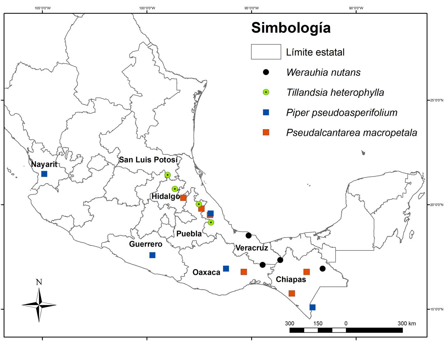
En el presente trabajo se reportan por primera vez las Bromeliaceae epífitas Pseudalcantarea macropetala para Hidalgo, Tillandsia heterophylla para San Luis Potosí y Werauhia nutans para Tabasco, y Piper pseudoasperifolium para Veracruz, también se presenta un mapa de la distribución de las 4 especies en México.
Materiales y métodos
Como parte de un taller de divulgación científica en Hidalgo (Tenango de Doria, Centro Ecoturístico “Agua Viva”, 17º21’51” N, 93º37’34” O), exploraciones botánicas en San Luis Potosí (Xilitla, camino a La Silleta, 21º26’20” N, 99º00’30” O) y Tabasco (Villa de Guadalupe, 17º21’51” N, 93º37’34” O), y dentro del proyecto “Funcionalidad socioecológica de áreas verdes urbanas neotropicales en Veracruz” (Jardín Botánico Francisco Javier Clavijero (19º30’53” N, 96º58’36” O), Xalapa y área natural protegida (ANP) La Martinica (19º34’20” N, 96º56’04” O), Banderilla, entre el 2018 y 2023, se colectaron varios especímenes de las familias Bromeliaceae y Piperaceae, entre ellas Pseudalcantarea macropetala, Piper pseudoasperifolium, Tillandsia heterophylla y Werauhia nutans. Si el ejemplar no se encontraba reproductivo, en el caso de las bromelias epífitas, se puso en cultivo en la localidad para su monitoreo hasta el desarrollo completo de la inflorescencia. El material colectado se procesó y se determinó usando claves de identificación taxonómica y monografías de ambos grupos (Espejo-Serna et al., 2005, 2021; Samain y Tebbs, 2020; Tebbs, 1993) y revisión de los herbarios CIB, HEM, MEXU y XAL (acrónimos de acuerdo a Thiers [2016]). Adicionalmente, se revisaron los trabajos de Tebbs (1993); Espejo-Serna et al. (2005, 2021) y para la distribución, se consultaron listados florísticos (Espejo-Serna y López-Ferrari 2004; Espejo-Serna et al., 2005, 2021; Villaseñor, 2016) y bases de datos, Portal de Datos Abiertos UNAM (UNAM, 2022) y Missouri Botanical Garden (TROPICOS, 2022).
Usando la información de un espécimen por estado (tabla 1), se elaboró un mapa de distribución de las 4 especies en México, Pseudalcantarea macropetala: P. A. Aguilar-Rodríguez PA001 (CITRO), P. A. Aguilar-Rodríguez et al. PA0022 (HEM), A. Espejo et al. 6700 (UAMIZ), J. Martínez Meléndez 1785 (HEM), F. Ventura A. 1061 (MEXU); Piper pseudoasperifolium: J. S. Miller et al. 2715 (MO), G. Flores F. y R. Ramírez R. 2514 (MO), R. Torres C. y A. Campos V. 10697 (MO), Calónico-Soto 8878 (MEXU), P. A. Aguilar-Rodríguez PA0025 (HEM); T. heterophylla: J. Ceja et al. 1869 (IEB, UAMIZ), A. Mendoza R. et al. 691 (UAMIZ), T. B. Croat 39637 (MO), M. A. Pérez-Farrera et al. 4019 (HEM); Werauhia nutans: E. Martínez S. y M. A. Soto A. 18654 (MEXU), P. Tenorio y T. Wendt 19335 (UAMIZ), P. A. Aguilar-Rodríguez et al. PA0014 (HEM), P. A. Aguilar-Rodríguez PA0012 (CITRO).
Todo el material colectado se etiquetó y se depositó en el herbario HEM. La identificación de Piper pseudoasperifolium fue corroborada por el especialista en la familia Piperaceae, Ricardo Callejas Posada, del Instituto de Biología, Universidad de Antioquia, Medellín, Colombia.
Resultados
Pseudalcantarea macropetala (Wawra) Pinzón et Barfuss. Fig. 1A.
Hierba epífita, raramente rupícola, arrosetada, de hasta 175 cm de alto, solitaria, con láminas acintadas, de entre 45 y 50 cm de largo, punctulado-lepidotas en el haz y envés, erectas a ascendentes. Inflorescencias terminales, erectas, compuestas, raramente simples, con hasta 7 espigas y un escapo de cerca de 80 cm de largo, cubierto por brácteas imbricadas. Cada espiga contiene hasta 20 flores, con disposición dística y actinomorfas, pétalos color verde claro en antesis, acintados y enrollados en el extremo sobre sí mismos, de hasta 12.3 cm de largo y los estambres subiguales. Cápsulas y semillas fusiformes, estas últimas con un apéndice plumoso blanco. La floración de esta especie ocurre de diciembre a abril, según la localidad, presenta antesis nocturna y sus flores son polinizadas por murciélagos (citada como Tillandsia macropetala; Aguilar-Rodríguez et al., 2014; Krömer et al., 2012). Es posible que se distribuya hasta Centroamérica (Krömer et al., 2012), pero en México, se distribuye en Chiapas, Hidalgo, Oaxaca, Puebla y Veracruz (fig. 2). Crece en bosque tropical subcaducifolio y bosque mesófilo de montaña, entre 1,200 y 2,500 m snm (Espejo-Serna et al., 2021).
Ejemplar examinado: México. Hidalgo, municipio Tenango de Doria, Centro Ecoturístico “Agua Viva”, 20°20’15.93” N, 98°15’29.38” O, 1,395 m, 29.X.2021, P. A. Aguilar-Rodríguez et al. PA0022 (HEM).
Tillandsia heterophylla É. Morren, Belgique Hort. 23: 138. 1873. Tipo: México, Veracruz, aux environs de Córdoba “Cordova”. O. Malzine s. n. (Holotipo: LG). Fig. 1B.
T. virginalis É. Morren, Belgique Hort. 30: 238-240. 1880, nom. illeg.
Hierba epífita arrosetada, glauca, pruinosa de hasta 150 cm de alto, solitaria, con láminas de las hojas acintadas de cerca de 30 a 40 cm de largo, de color verde o teñido de púrpura, punctulado-lepidotas en el haz y envés, acuminadas y erecto-extendidas al ápice. Inflorescencias terminales, erectas, compuestas, a veces simples, con hasta 16 espigas pruinosas y un escapo de hasta 80 cm, cubierto desde la base al ápice por las vainas de las brácteas. Las flores son tubular-campaniformes, con pétalos blancos y estambres más cortos que los pétalos. Cápsulas rostradas y semillas fusiformes, con un apéndice plumoso blanco. Su floración ocurre de febrero a julio, con antesis nocturna a brevemente diurna y sus flores son polinizadas por murciélagos, polillas, colibríes y abejas (Aguilar-Rodríguez et al., 2016; Espejo-Serna et al., 2005). Se le considera endémica de México y se distribuye en Hidalgo, Puebla, San Luis Potosí y Veracruz (fig. 2). Crece en bosque de Quercus y bosque mesófilo de montaña, entre 600 y 1,700 m snm (Espejo-Serna et al., 2005, 2021).
Figura 1. A, Pseudalcantarea macropetala con inflorescencia; B, Tillandsia heterophylla con inflorescencia en desarrollo; C, Werauhia nutans con inflorescencia en desarrollo; y D, Piper pseudoasperifolium con inflorescencia.
Ejemplar examinado: México. San Luis Potosí, municipio Xilitla, camino a La Silleta, 21°25’45” N, 99°00’38” O, 750 m, 31.VII.2021, M. A. Pérez-Farrera et al. 4019 (HEM).
Vriesea nutans L. B. Sm., Phytologia 7(4): 175. 1960. Tipo: Costa Rica, San José, road from Turrialba to Moravia, M. B. Foster 2727 (holotipo: US)
Hierba epífita, arrosetada, de hasta 60 cm de alto, solitaria pero frecuente que forme agrupaciones de varios individuos, con láminas de las hojas acintadas de cerca de 40 cm de largo, punctulado-lepidotas, glabrescentes en haz y envés, agudas a atenuadas en el ápice. Las inflorescencias son terminales con un escapo delgado, de hasta 3 mm de diámetro y de hasta 45 cm de largo, cubierto en toda su longitud por las vainas de las brácteas, las espigas alcanzan hasta 12.5 cm de largo con 5-9 flores con un arreglo dística y zigomorfas, brácteas florales quebradizas cuando están secas. Flores con pétalos blancos y estambres desiguales más corto que los pétalos. Cápsulas pardas oscuras, fusiforme, de hasta 3.3 cm de largo con semillas de hasta 4 mm de largo, con un apéndice plumoso. Su floración ocurre de octubre a diciembre, presenta antesis nocturna y se reproduce por autopolinización y clonación (Aguilar-Rodríguez et al., 2019; Espejo-Serna et al., 2005). Se distribuye desde México hasta Costa Rica. En México ha sido colectada en Oaxaca, Chiapas, Tabasco y Veracruz (fig. 2). La especie crece en bosque tropical perennifolio y bosque mesófilo de montaña, entre 100 y 1,100 m snm (Espejo-Serna et al., 2005, 2007, 2021).
Tabla 1
Sitios de colecta de ejemplares de Pseudalcantarea macropetala, Tillandsia heterophylla, Werauhia nutans y Piper pseudoasperifolium revisadas en el artículo y representadas en la figura 2; se incluyen las localidades de los nuevos registros estatales (en negritas). Abreviaturas de los estados: CHI (Chiapas), GUE (Guerrero), HID (Hidalgo), NAY (Nayarit), OAX (Oaxaca), PUE (Puebla), SLP (San Luis Potosí), TAB (Tabasco), VER (Veracruz).
Estados
Especie (familia)
Pseudalcantarea macropetala (Bromeliaceae)
Tillandsia heterophylla (Bromeliaceae)
Werauhia nutans (Bromeliaceae)
Piper pseudoasperifolium (Piperaceae)
CHI
J. Martínez Meléndez 1785 (HEM), 15°45’39” N 093°04’19” O
E. Martínez S. y M. A. Soto A. 18654 (MEXU), 16°57’15” N 091°35’49” O
J. S. Miller et al. 2715 (MO), 15°06’00” N 092°04’48” O
GUE
Calónico-Soto 8878 (MEXU), 17°35’33” N 099°44’27” O
HID
P. A. Aguilar-Rodríguez et al. PA0022 (HEM), 20º20’15.93” N, 98º15’29.38” O
J. Ceja et al. 1869 (IEB, UAMIZ), 20°45’52” N 098°39’53” O
NAY
G. Flores F. y R. Ramírez R. 2514 (MO), 21°29’N 104°55’W
OAX
A. Campos V. y R. Torres C. 3614 (HEM, MEXU), 16°47’16” N 095°21’59” O
P. Tenorio y T. Wendt 19335 (UAMIZ), 17°08’ N 94°28’ O
R. Torres C. y A. Campos V. 10697 (MO), 16°57’00” N 096°13’00” O
PUE
F. Ventura A. 1061 (MEXU), 19°49›20” N 097°23’51” O
A. Mendoza R. et al. 691 (UAMIZ), 20°01’58” N 097°31’07” O
SLP
M. A. Pérez-Farrera et al. 1056 (HEM), 21°25’45” N, 99°00’38” O
TAB
P. A. Aguilar-Rodríguez et al. PA0015 (HEM), 17º21’51’’ N, 93º37’34’’ W
VER
P. A. Aguilar-Rodríguez PA001 (CITRO), 19°31’12” N 096°59’17” O
T. B. Croat 39637 (MO), 19°09’36” N 096°56’24” O
P. A. Aguilar-Rodríguez PA0012 (CITRO) 18°32’03” N 095°08’18” O
P. A. Aguilar-Rodríguez et al. PA0025 (HEM), 19°35’23” N 096°57’01” O
Ejemplar examinado: México. Tabasco, municipio Huimanguillo, Cerro de las Flores, Villa de Guadalupe, 17°21’51” N, 93°37’34” O, 1,024 m, 7.V.2018, P. A. Aguilar-Rodríguez et al. PA0014 (HEM).
Figura 1. A, Pseudalcantarea macropetala con inflorescencia; B, Tillandsia heterophylla con inflorescencia en desarrollo; C, Werauhia nutans con inflorescencia en desarrollo; y D, Piper pseudoasperifolium con inflorescencia.
Piper pseudoasperifolium C. DC., Prodr. 16(1): 318 (1869). Isotipo: México, Oaxaca, Franco s. n. (G-DC). Fig. 1D.
Arbusto de hasta 5 m de altura, con tallos y peciolos densamente pubescentes. Hojas ovado-lanceoladas a elíptico-lanceoladas, buliformes, glandulosas, con el haz escabroso y el envés densamente pubescente sobre los nervios. Inflorescencias con pedúnculos pubescentes, erectas y tienen menos de 10 cm de largo; los frutos son redondos y glabros, verde claro, de entre 3 y 6 cm de largo. Crece principalmente en bosque mesófilo de montaña, en matorrales y en pinares, entre 0 y 2,010 m snm. Se distribuye de México a Costa Rica (Callejas-Posada, 2020; Tebbs, 1993). Su floración ocurre todo el año (PA Aguilar-R., obs. pers.) y la información sobre su biología reproductiva es desconocida. En México esta especie solo había sido registrada para Chiapas, Guerrero, Jalisco, Nayarit y Oaxaca (fig. 2). Crece en bosque húmedos tropicales, entre 300 y 1,400 m snm (Callejas-Posada, 2020; Villaseñor, 2016).
Figura 2. Presencia en México de algunos ejemplares representativos para la distribución nacional de Pseudalcantarea macropetala cuadros en naranja), Tillandsia heterophylla (círculos verdes), Werauhia nutans (círculos negros) y Piper pseudoasperifolium (cuadros azules), en México. Las coordenadas de los ejemplares colectados se encuentran en la tabla 1.
Ejemplares examinados: México. Veracruz, municipio Banderilla, Área Natural Protegida, La Martinica, 19°35’23” N, 96°57’01” O, 1,543 m, 25.III.2023, P. A. Aguilar-Rodríguez PA0025 (HEM); municipio Xalapa, Jardín Botánico Francisco Javier Clavijero, 19°30’50” N, 96°56’38” O, 1,320 m snm, 25.III.2023, P. A. Aguilar-Rodríguez PA0023 (HEM).
Discusión
El hallazgo de estas 4 especies de plantas en estados con inventarios florísticos recientes (p.e., Tobías-Baeza et al., 2019; Torres-Colín et al., 2017; Vargas-Rueda et al., 2019; Villaseñor et al., 2022) demuestra la importancia de continuar realizando exploraciones y colectas en los diferentes tipos de vegetación de México, pero particularmente en el bosque mesófilo de montaña (solamente T. heterophylla fue colectada en un bosque de encino), uno de los tipos de vegetación en México con una alta diversidad florística (hasta 6,790 spp.; Villaseñor, 2010) y donde la mayoría de las especies reportadas en este estudio fueron encontradas, así como en los fragmentos boscosos urbanos.
Además, las Bromeliaceae Pseudalcantarea macropetala, para Hidalgo, Tillandsia heterophylla para San Luis Potosí, corresponden a los registros más norteños para estas especies con distribución exclusiva en México. Aunque probablemente la primera especie tenga una presencia en Centroamérica, aún no se han analizado ejemplares de herbario de Pseudalcantarea viridiflora, toda vez que hay ejemplares entremezclados de ambas especies en diferentes herbarios (PA Aguilar-R, obs. pers.).
Pseudalcantarea grandis (Schltdl.) Pinzón et Barfuss y P. viridiflora (Beer) Pinzón et Barfuss, son las otras 2 especies del género presentes en México, ambas también se encuentran en Hidalgo (Espejo-Serna et al., 2005, 2021). El registro de P. macropetala representa la tercera especie del género para el estado, mientras que el reporte de Tillandsia heterophylla para San Luis Potosí aumenta el número a 20 spp. dentro del género en el estado (Espejo-Serna et al., 2021). Anteriormente, T. heterophylla se había reportado solo para Hidalgo, Puebla y Veracruz (Espejo-Serna et al., 2005, 2021). El espécimen Reyes-García 6495 (MEXU, MO) colectado en Chiapas y determinado como T. heterophylla debe ser analizado para confirmar su determinación. La especie es abundante en los sitios donde se encuentra y parece seguir una distribución a través de la provincia biogeográfica de la Sierra Madre Oriental (sensu Morrone et al., 2002), por lo que, hipotetizamos, que al menos en el sur de Tamaulipas, pueda estar presente esta especie en hábitats boscosos.
Por otro lado, en este estudio se confirma la presencia de W. nutans para Tabasco, confirmando su presencia en otra localidad de la provincia biogeográfica Veracruzana (sensu Morrone et al., 2002) (tabla 1) y representa la tercera especie del género para el estado, ya que previamente se había reportado W. gladioliflora (H. Wendl.) J.R. Grant (Espejo-Serna et al., 2005, 2021) y W. maculata Espejo-Serna, López-Ferrari, Aguilar-Rodr., Diaz Jim. (Aguilar-Rodríguez et al., 2020).
El reporte de Piper pseudoasperifolium como nuevo registro para Veracruz eleva el número a 90 spp. del género Piper en el estado, lo cual representa 66% de las 136 spp. reportadas en México (Villaseñor, 2016). En la revisión de herbarios y bases de datos se pudo constatar que, a diferencia de otras especies de Piper (p.e., P. aduncum L., P. amalago L., P. hispidum Sw.), P. pseudoasperifolium ha sido poco recolectada en México, con menos de 17 especímenes registrados en Chiapas, 3 en Oaxaca, 2 en Nayarit y 1 en Guerrero, abarcando varias provincias biogeográficas con distintas características, como la del Balsas, Tierras bajas del Pacífico, Veracruzana y de la Sierra Madre del Sur (sensu Morrone et al., 2002). Esto sugiere que esta especie también tendrá presencia en Jalisco, Michoacán y quizá Colima, siendo así una especie con representación en las regiones neártica y neotropical. En Veracruz, esta especie se recolectó en el Jardín Botánico Francisco Javier Clavijero, en el municipio de Xalapa y en el Área Natural Protegida La Martinica, en Banderilla, como parte del proyecto “Funcionalidad socioecológica de áreas verdes urbanas neotropicales en Veracruz”. En ambos sitios, P. pseudoasperifolium crece abundante, tanto en la orilla del bosque, como en el sotobosque y simpátrica con otras especies del mismo género como P. auritum y P. lapathifolium (PA Aguilar-R pers. obs.), lo que sugiere una especie con una gran adaptabilidad a la perturbación antrópica y que crece en simpatría con otras especies morfológicamente muy similares.
Agradecimientos
A Pedro Díaz Jiménez, Melany Aguilar López, Mané Salinas Rodríguez, Diego A. Báez Ruiz, y Rocío Cárcamo Corona por su ayuda en campo y al procesar las muestras; a Ricardo Callejas-Posada por su valiosa ayuda en la identificación Piper. A Adolfo Espejo-Serna por su ayuda para la revisión de especímenes. Y a Mauricio Gerónimo Martínez-Martínez y Melany Aguilar López por la elaboración del mapa. Algunas salidas de campo fueron solventadas por parte del proyecto de Ciencia Básica del Conahcyt “Funcionalidad socioecológica de áreas verdes urbanas neotropicales” (64358).
Referencias
Aguilar-Rodríguez, P. A., Díaz-Jiménez, P., Espejo-Serna, A., López-Ferrari, A. R., Hentrich, H., Yovel, Y. et al. (2020). A new Werauhia (Tillandsioideae, Bromeliaceae) from Mexico with observations about its reproductive biology. Phytotaxa, 446, 128–134. https://doi.org/10.11646/phytotaxa.446.2.6
Aguilar-Rodríguez, P. A., Krömer, T., García-Franco, J. G. y MacSwiney G., M. C. (2016). From dusk till dawn: nocturnal and diurnal pollination in the epiphyte Tillandsia heterophylla (Bromeliaceae). Plant Biology, 18, 37–45. https://doi.org/10.1111/plb.12319
Aguilar-Rodríguez, P. A., MacSwiney G., M. C., Krömer, T., García-Franco, J. G., Knauer, A. y Kessler, M. (2014). First record of bat-pollination in the species-rich genus Tillandsia (Bromeliaceae). Annals of Botany, 113, 1047–1055. https://doi.org/10.1093/aob/mcu031
Aguilar-Rodríguez, P. A., Tschapka, M., García-Franco, J. G., Krömer, T. y MacSwiney G., M. C. (2019). Bromeliads going batty: pollinator partitioning among sympatric chiropterophilous Bromeliaceae. AoB Plants, 11, 1–19. https://doi.org/10.1093/aobpla/plz014
Barfuss, M. H. J., Till, W., Leme, E. M. C., Pinzón, J. P., Manzanares, J. M., Halbritter, H. et al. (2016). Taxonomic revision of Bromeliaceae subfam. Tillandsioideae based on a multi- locus DNA sequence phylogeny and morphology. Phytotaxa, 279, 1–97. https://doi.org/10.11646/phytotaxa.279.1.1
Benzing, D. H. (2000). Bromeliaceae. Profile of an adaptive radiation. Cambridge, RU: Cambridge University Press.
Espejo-Serna, A. y López-Ferrari, A. R. (2004). Notas sobre la familia Bromeliaceae en el Valle de México. ActaBotanica Mexicana, 67, 49–57. https://doi.org/10.21829/abm67.2004.973
Espejo-Serna, A., López-Ferrari, A. R. y Ramírez-Morillo, I. (2005). Bromeliaceae. Flora de Veracruz. Fascículo 136. Xalapa: Instituto de Ecología, A.C.
Espejo-Serna, A., López-Ferrari, A. R., Martínez-Correa, N. y Pulido Esparza, V. A. (2007). Bromeliad flora of Oaxaca, Mexico: Richness and distribution. Acta Botanica Mexicana, 81, 71–147. https://doi.org/10.21829/abm81.2007.1025
Espejo-Serna, A., López-Ferrari, A. R., Mendoza-Ruiz, A., García-Cruz, J., Ceja-Romero, J. y Pérez-García, B. (2021). Mexican vascular epiphytes: richness and distribution. Phytotaxa, 503, 001–124. https://doi.org/10.11646/phyto taxa.503.1.1
Krömer, T., Espejo-Serna, A., López-Ferreri, A. R., Ehlers, R. y Lautner, J. (2012). Taxonomic and nomenclatural status of the Mexican species in the Tillandsia viridiflora complex (Bromeliaceae). Acta Botanica Mexicana, 99, 1–20. https://doi.org/10.21829/abm99.2012.16
Morrone, J., Espinosa-Organista, D. y Llorente-Bousquets, J. (2002). Mexican biogeographic provinces: preliminary scheme, general characterizations, and synonymies. Acta Zoológica Mexicana, 85, 83–108. https://doi.org/10.21829/azm.2002.85851814
Quijano-Abril, M. A., Callejas-Posada, R. y Miranda-Esquivel, D. R. (2006). Areas of endemism and distribution patterns for Neotropical Piper species (Piperaceae). Journal of Biogeography, 33, 1266–1278. https://doi.org/10.1111/j.1365-2699.2006.01501.x
Samain, M. S. y Tebbs, M. C. (2020). Piperaceae. Flora del Bajío y de Regiones Adyacentes, 215, 1–62.
Tebbs, M. C. (1993). Revision of Piper in the new in the New World. 3. The taxonomy of Piper sections Lepiantes and Radula. Bulletin of the Natural History Museum of London, 23, 1-50.
Thiers, B. (2016) Index Herbariorum. A global directory of public herbaria and associated staff. New York Botanical Garden`s virtual herbarium. https://sweetgum.nybg.org/science/ih/
Tobías-Baeza, A., Salvador-Morales, P., Sánchez-Hernández, R., Ruiz-Acosta, S. C., Arrieta-Rivera, A. y Andrade-Prado, H. (2019). Composición florística y carbono en la vegetación arbórea de un área periurbana en Tabasco, México. Ecosistemas y Recursos Agropecuarios, 6, 369–376. https://doi.org/10.19136/era.a6n17.2009
Torres-Colín, R., Parra, J. G., de la Cruz, L. A., Ramírez, M. P., Gómez-Hinostrosa, C., Bárcenas, R. T. et al. (2017). Flora vascular del municipio de Guadalcázar y zonas adyacentes, San Luis Potosí, México. Revista Mexicana de Biodiversidad, 88, 524–554. https://doi.org/10.1016/j.rmb.2017.07.003
TROPICOS. (2022a). Missouri Botanical Garden. Recuperado el 10 de septiembre de 2022 de: https://www.tropicos.org/home
Vargas-Rueda, A. F., Rivera-Hernández, J. E., Cházaro-Basáñez, M. J. y Alcántara-Salinas, G. (2019). Nuevos registros para la flora de Veracruz en el Parque Nacional Cañón del Río Blanco, México. Acta Botanica Mexicana, 126, e1429. https://doi.org/10.21829/abm126.2019.1429
Villaseñor, J. L. (2010). El bosque húmedo de montaña en México y sus plantas vasculares. Catálogo florístico taxonómico. Ciudad de México: Conabio/ UNAM.
Villaseñor, J. L. (2016). Checklist of the native vascular plants of Mexico. Revista Mexicana de Biodiversidad, 87, 559–902. https://doi.org/10.1016/j.rmb.2016.06.017
Villaseñor, J. L., Ortiz, E. y Sánchez-González, A. (2022). Riqueza y distribución de la flora vascular del estado de Hidalgo, México. Revista Mexicana de Biodiversidad, 93, e933920. https://doi.org/10.22201/ib.20078706e.2022.93.3920
Zotz, G. (2013). The systematic distribution of vascular epiphytes —a critical update. Botanical Journal of the Linnean Society, 171, 453–481. https://doi.org/10.1111/boj.12010
Universidad Nacional Autónoma de México, Facultad de Ciencias, Departamento de Biología Evolutiva, Laboratorio Biogeografía de la Conservación, Circuito Exterior s/n, Ciudad Universitaria, Coyoacán, 04510 Ciudad de Mëxico, Mexico
The Transmexican Volcanic Belt (TVB) is a complex biogeographical province characterized by several areas of endemism and high diversity of flora and fauna produced by complex geological and evolutionary processes. Chorotypes are biogeographical patterns that occur either when 2 or more independently distributed species share the same occupied area, or even when a single species’ distribution area differs significantly from others. Here, we identified chorotypes of 167 endemic species inhabiting the TVB using geographic distribution models and quantitative methods. Of those species, 136 were included in 11 chorotypes, named I to XI. In addition, the insect Aedes niveoscotum constituted chorotype XII. The 30 remaining species did not belong to any chorotype. All chorotypes included species from different taxonomic groups, which may be due to a shared biogeographical history. The chorotypes with the highest richness were located in the central and eastern TVB, suggesting that volcano peaks and surrounding areas are important for generating the particular environmental conditions that restrict the distribution of species of different taxonomic groups.
Keywords: Biogeography; Patterns; Similarity; Species richness; Species distribution models
Corotipos y relaciones geográficas entre especies endémicas de la Faja Volcánica Transmexicana, México
Resumen
La Faja Volcánica Transmexicana (FVT) es una provincia biogeográfica compleja caracterizada por varias áreas de endemismo y una alta diversidad de flora y fauna, producto de complejos procesos geológicos y evolutivos. Los corotipos son patrones biogeográficos que ocurren cuando 2 o más especies de distribución independiente comparten la misma área de ocupación, o incluso cuando la distribución de una única especie difiere significativamente de otras. En este manuscrito, nosotras identificamos corotipos para 167 especies endémicas que habitan la FVT usando modelos de distribución geográfica y métodos cuantitativos. A partir del total de especies, 136 estuvieron incluidas en 11 corotipos, nombrados del I al XI. Adicionalmente, el insecto Aedes niveoscotum conformó el corotipo XII. Las 30 especies restantes no pertenecieron a ningún corotipo. Todos los corotipos incluyeron especies de diferentes grupos taxonómicos, lo cual puede deberse a una historia biogeográfica común. Los corotipos con la mayor riqueza de especies estuvieron localizados en el centro y este de la FVT, sugiriendo que los picos de los volcanes y las áreas circundantes son importantes para producir las condiciones ambientales particulares que restringen la distribución de las especies de diferentes grupos taxonómicos.
Palabras clave: Biogeografía; Patrones; Similitud; Riqueza de especies; Modelos de distribución de especies
Introduction
Distributional patterns in biogeography occur when a group of species share a given geographic space; while species that are distributed independently from each other show no distributional pattern (Márquez et al., 1997). The word “chorotype” was introduced by La Greca in 1963 (La Greca, 1963, in Morrone, 2014). According to Fattorini (2016), the term chorotype was implicitly used by La Greca to refer to “chorological categories”. Years later, an equivalence between chorological category and chorotype was established (Fattorini, 2016), defining a chorotype as the coincidence between the distribution ranges of species. Numerical chorotypes were defined by Baroni-Urbani et al. (1978) as a biogeographic pattern of 2 or more species occupying a similar area (Barbosa & Estrada, 2016; Real, Guerrero, & Vargas, 1992; Vargas & Real, 1997). Moreover, according to Real et al. (1996), the distribution area of a single species can be considered a chorotype if the distribution is significantly different from the distributions of other species. Because the identification of patterns using subjective methods can lead to mistaken results (Flores et al., 2004; Jardine, 1972; Márquez et al., 1997), it has been necessary to use quantitative techniques such as the appropriate similarity indices to produce coherent and reproducible results (Márquez et al., 1997). These techniques should compare the species’ distributions and their groupings in chorotypes (Barbosa & Estrada, 2016).
Similarity among species distributions has been analyzed from different perspectives. The Jaccard index (1908) has been used to compare the presence of species between 2 communities (Mostacedo & Fredericksen, 2000), but considers only presence data; it does not take into account the double absence of species. Real, Guerrero, and Ramírez (1992), and Real and Vargas (1996) consider this an advantage because the similarity between the 2 sites is not influenced by the number of other sites studied. However, Rice and Belland (1982) discussed that high or low values of Jaccard’s index could be random. Conversely, Baroni-Urbani and Buser (1976) proposed an index considering double absences, since 2 species could be absent from a locality due to ecological and historical reasons or inadequate sampling. Moreover, shared absences between species can be interpreted as coinciding distribution limits, like biogeographic barriers (Flores et al., 2004). For this index, there is a statistical table of associated probabilities (Baroni-Urbani & Buser, 1976). Later, Buser and Baroni-Urbani (1982) and Real, Guerrero, and Ramírez (1992) suggested caution in interpreting analyses that consider double absences, since including additional localities can alter the results of the index. Therefore, Real, Guerrero, & Vargas (1992) consider to Buser and Baroni-Urbani index as a feature of a relationship in the context of all the sites analyzed.
The Transmexican Volcanic Belt (TVB) is a complex mountainous biogeographical province between the Nearctic and Neotropical regions (Morrone et al., 2017). The TVB is located between 19-20° North latitude. It spans of 1,000 km and crosses Mexico in an east-west direction. This province is characterized by several areas of endemism and a high diversity of flora and fauna, produced by complex geological and biological processes (Hernández & Carrasco, 2007; Ruggiero & Ezcurra, 2003; Suárez-Mota et al., 2013). The TVB has the most heterogeneous relief and the highest elevations in Mexico, with important changes in altitude over short distances. This results in high climatic diversity between highland and lowland areas, which promotes high species richness (Hernández & Carrasco, 2007). The highest mountains in Mexico are in the TVB, including the Pico de Orizaba (5,650 m of altitude), Popocatépetl (5,450 m), Iztaccíhuatl (5,280 m), Nevado de Toluca (4,560 m), Malinche (4,460 m) and Nevado de Colima (4,340 m) (Suárez-Mota et al., 2013).
Non-random historical relationships could explain the biogeographic patterns displayed by the species of the TVB because they evolved under similar environmental conditions (Frey, 1992). Unfortunately, environmental deterioration resulting from the expansion of human activities has a negative effect on the habitat of many species distributed in the TVB. To contribute to the knowledge of biogeographical patterns in the TVB, we aimed to identify chorotypes of endemic species of 5 different taxa (amphibians, birds, insects, mammals and plants) using species distribution models and quantitative methods.
Materials and methods
We compiled a database of 167 endemic species of the TVB belonging to 5 taxonomic groups (Supplementary material: Table S1.1): 25 species of amphibians (Flores-Villela et al., 2010); 1 bird (Navarro-Sigüenza et al., 2003; Peterson et al., 2016); 89 species of insects (GBIF, 2017; Reyes-Castillo & Morón Ríos, 2005; SNIB-Conabio, 2017), 15 mammals (Escalante, 2015); and 37 plants (Magnoliopsida) (Escalante, 2015; Hernández & Gómez-Hinostrosa, 2011, 2015; Téllez-Valdés, 2017). These taxa were selected using their data points of occurrence from a previous database (Escalante et al., 2020; Supplementary material: Fig. S1.1), where at least 50% of the presence points for each species fell within the TVB polygon (Morrone et al., 2017).
To obtain the distribution areas of species, we generated species distribution models (SDM) for the 43 species with at least 6 data points using Maxent 3.4.0 (Phillips et al., 2017). SDM allow to predict the spatial distribution of a species based on statistical relationships between their occurrences and environmental conditions, producing a comprehensive understanding of the factors that molded species presence (Elith & Leathwick, 2009; Elith et al., 2006). The species distribution models were produced as in Escalante et al. (2020). Maxent was run using the ‘dismo’ package (Hijmans et al., 2017) in R version 3.4.2 (R Core Team, 2017) and we applied the omission error threshold of E = 10 (Peterson et al., 2008) to transform model output to binary. For the other 124 species (which had 5 or fewer data points or poor model performance), the geographic distribution was obtained directly from the data points.
Each species distribution model and geographic distribution was overlapped with a 0.5° latitude-longitude grid in QGIS v. 2.18.6 (QGIS Development Team, 2016) to determine the presence of a species in each cell of the grid. We built a presence-absence matrix for all species, where a species’ presence in each grid cell was coded as ‘1’ and absence as ‘0’. Based on the presence-absence matrix of 167 species and 609 cells, we applied the Baroni-Urbani and Buser index (1976) to obtain the similarity between the distributions of each pair of species. The index is as follows:
where A is the number of cells in which species “a” is present, B is the number of cells in which species “b” is present, C is the number of cells where both species “a” and “b” are present, and D is the number of cells in which both species “a” and “b” are absent. Because the double absences could lead to apparent similarity between 2 geographic distributions, they are multiplied by the double presences (Marquez et al., 1992). This could also prevent the effect of the Wallacean shortfall —i.e., lack of distribution data; Hortal et al., 2015— on some species, particularly those whose distributions were taken directly from points rather than modeled.
We identified chorotypes using the “Rmacoqui” package (Olivero et al., 2015) in R v.1.0.143 (R Core Team, 2017). Although all processes were developed in the R script, we describe the step-by step following: first, there was a transformation of the similarity matrix into a significant similarity matrix of ‘+’, ‘-’ and ‘0’ values, following to Márquez et al. (1997). Next, a cluster analysis was performed using the UPGMA (Unweighted Pair-Group Method using Arithmetic Averages) hierarchical classification method. For each cluster, we tested for significant segregation following McCoy et al. (1986). For each bifurcation in the dendrogram, a submatrix was developed, in which there are 3 zones with values that relate the species’ distributions: 1) “AxA zone”, including the values that related the “A group”; 2) “BxB zone”, which includes the values that related to the distributions of the “B group”; and 3) “AxB zone”, where the values related the “A group” with the “B group” distributions.
To evaluate whether the degree of similarity was higher than expected at random, we applied the DW parameter (McCoy et al., 1986). DW(AxA) quantifies the degree to which the major similarities (‘+’) are greater than expected at random in the “AxA zone”, but they are not in the “AxB zone”, at the same time that the minor similarities (‘-’) are absent from “AxA zone” (Real et al., 2003). DW(BxB) is analogous to DW(AxA), and both DW parameters contain all necessary conditions to determine whether A or B distributions belong to a chorotype. Therefore, we identified a chorotype when DW(AxA) and DW(BxB) were higher than 0.447 for all geographic distributions in the group (Real et al., 2003). Moreover, we applied the additional parameter GW to evaluate whether the segregation between the A and B groups was weak (Márquez et al., 1997). Finally, we calculated the DS parameter (Real et al., 2003), which determines whether the similarity was less than expected at random in the “AxB” zone, but not in the “AxA” and “BxB” zones, as well as whether higher-than-random similarities are absent in the “AxB” zone. The statistic test for DS was GS (McCoy et al., 1986). Therefore, a group was considered a chorotype if its DW was higher than ‘0’ and its corresponding statistic GW was significant.
In connection with that, we identified the least fuzzy chorotypical clusters, where all the conditions of a chorotype are maximized; however, a chorotypical cluster is neither true nor false, but accurate to some extent (Olivero et al., 2011). Moreover, certain fuzzy clusters may be nested within others, although it is always possible to identify the non-nested fuzzy chorotypes. Therefore, we applied the following fuzzy parameters to the least fuzzy chorotypes identified the degree of membership in the intersection between 2 chorotypes that indicates pairwise coincidences in the species membership (cardinality), and the fuzzy overlap that measures the proportion of the union that is in the intersection (Olivero et al., 2011).
Finally, we projected the grid and data points with the presence of each species for each chorotype using QGIS (QGIS Development Team, 2016) to locate each chorotype in the geographic space.
Results
We obtained a significant similarity matrix for the 167 species (available as Excel file in Supplementary material or through the e-mail of the authors). According to this matrix, 11 chorotypes from 136 species could be identified, hereafter referred to as chorotypes I through XI. Moreover, 1 insect species (A. niveoscotum) was significantly different from the rest and, therefore, was assigned to its own possible chorotype (chorotype XII). The richest chorotype was VII, with 39 species containing 23% of the total species analyzed. The chorotypes with the least species were X (with 4 species, 2.39% of the total richness) and XII (1 species, 0.59%) (Table 1). Eighteen percent of the species (30) were not included in any of the chorotypes.
Table 1.
Number of species from each taxonomic group belonging to each chorotype (I-XII), total species richness, and richness as a percentage of the total species considered. The species that were not included in any chorotype are in the last row.
Chorotype
Number of species for each taxa
Richness
Richness percentage
Amphibians
Bird
Insects
Mammals
Plants
I
1
0
3
0
2
6
3.6
II
0
0
4
0
3
7
4.2
III
1
0
6
0
2
9
5.4
IV
2
0
11
0
1
14
8.4
V
1
0
7
0
1
9
5.4
VI
3
0
2
1
2
8
4.8
VII
6
1
11
7
14
39
23.3
VIII
1
0
5
0
0
6
3.6
IX
0
0
22
2
2
26
15.6
X
0
0
2
1
1
4
2.4
XI
0
0
6
0
2
8
4.8
XII
0
0
1
0
0
1
0.6
Remaining species
10
0
9
4
7
30
18
Figure 1. Simplified general dendrogram showing all chorotypes (I-XII). See figures S2.1 to S2.12 in Supplementary material to visualize in detail all the branches of each chorotype.
The general dendrogram included 12 sub-dendrograms, representing chorotypes I-XII (Fig. 1). All sub-dendrograms are shown in the Supplementary material (Figs. S2.1-S2.12). Chorotypes I, IV, VIII, and IX were located in the central and eastern part of the TVB (Figs. 2-4), chorotypes II, III, V and XI were located in the central TVB (Figs. 2, 3). Chorotype VI is located throughout the TVB, in the western, central and eastern parts (Fig. 3). In contrast to the rest, chorotype X was only in the eastern TVB (Fig. 5), and chorotype XII was located in the western TVB (Fig. 5).
Regarding the independence test GS, all species in chorotype IX had values above 0.5, except for species 95 (Aphodiusophistius), which had the lowest value (Supplementary material: Table S1.2). Chorotype XII had the highest membership value with a value of ‘1’ in the independence test. The fuzzy parameters that refer to including species within a chorotype are shown in Table 2, while the fuzzy overlap parameters are shown in Table 3. Inclusion (degree of integration in the intersection, likewise pairwise coincidences in the membership of the species) and overlap (which measures the proportion of the union that is found in the intersection) were related because the same chorotypic pairs had the highest values of both parameters (shown in bold; Tables 2, 3). In general, when we compared the inclusion values with the overlap values, we observed that the inclusion values were higher.
Discussion
We identified biogeographic patterns corresponding to chorotypes using the Baroni-Urbani and Buser (1976) index. The double absence component of this index was useful for our study area since the TVB has large mountain chains that have influenced species’ geographic distribution patterns. Consequently, geographic isolation could explain the absence or presence of different taxonomic groups in the TVB. In our particular dataset, the grouping of chorotypes was influenced by species distribution models versus individual data points, since using models generated larger chorotypes than the data points. These biases in data are named the Wallacean shortfall, defined as the lack of knowledge about the geographical distribution of the species (Hortal et al., 2015; Lomolino, 2004). Although in the last years have been published some contributions addressing how to deal with this shortfall (v. gr. Diniz-Filho et al., 2023), more research is necessary. As a result, we recommend that future analyses use only models or only data points for all species.
Figure 2. Cells of chorotypes I (3.6% of species richness), II (4.2%) and III (5.4%).
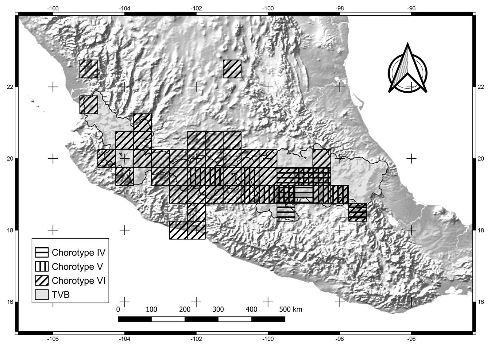
Figure 3. Cells of chorotypes IV (8.4% of species richness), V (5.4%) and VI (4.8%).
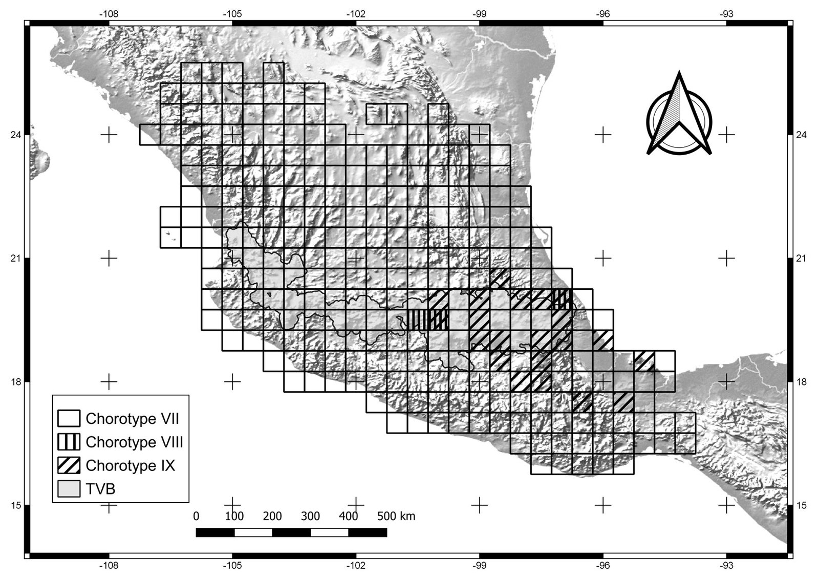
Figure 4. Cells of chorotypes VII (23.3% of species richness), VIII (3.4%) and IX (15.6%).
In general, similar analyses are generally performed within only one taxonomic group, e.g., amphibians (Flores et al., 2004; Olivero et al., 2011; Real, Guerrero, & Ramírez, 1992), plants (Gómez-González et al., 2004; Márquez et al., 1997), micro-mammals (Real et al., 2003) and birds (Real et al., 2008). Here, all 12 identified chorotypes included species from different taxonomic groups, which could be explained by similar geographic conditions resulting from a common biogeographic history of the species within a specific chorotype. Future analysis comparing other Operational Geographical Units and different scales could be necessary to evaluate the performance of the Baroni-Urbani and Buser (1976) index, which also could light about why some similar chorotypes are no grouped.
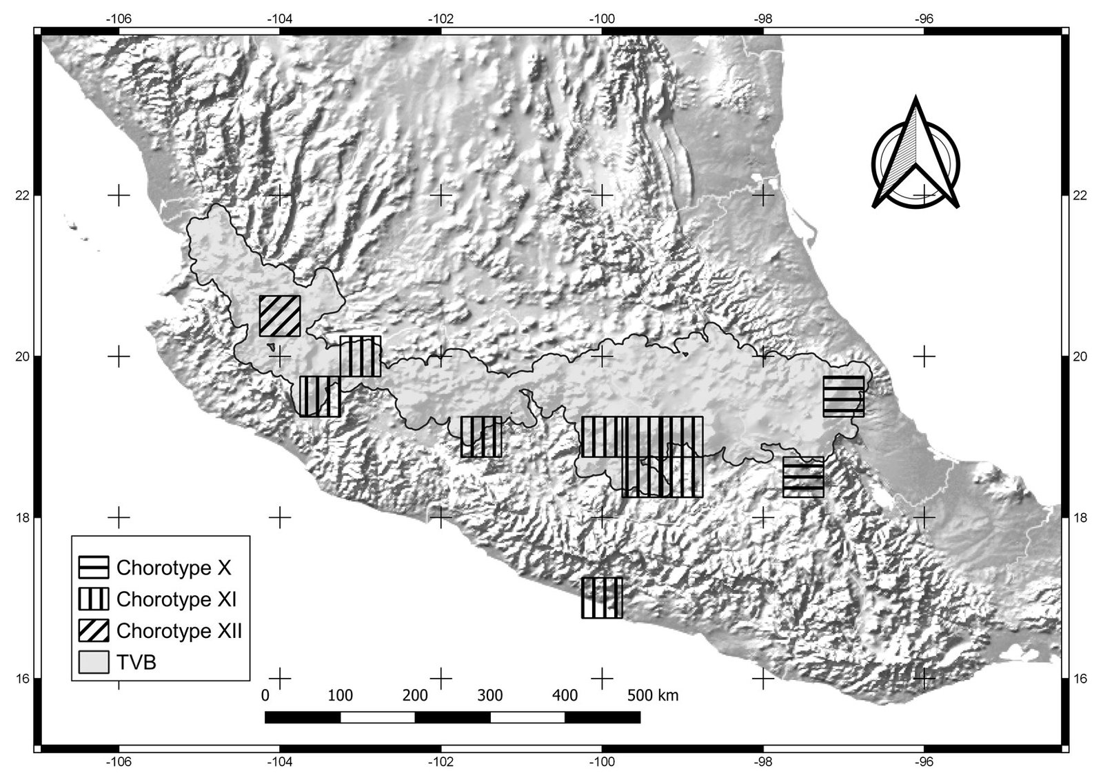
Figure 5. Cells of chorotypes X (2.4% of species richness), XI (4.8%) and XII (0.6%).
Table 2
Values that show the relationships between the chorotypes: inclusion of each chorotype regarding the rest according to cardinal parameter of fuzzy intersection between chorotypes. The bold numbers show the highest value in each column.
Chorotypes
Values of relationship between chorotypes
CI (In)
CII (In)
CIII (In)
CIV (In)
CV (In)
CVI (In)
CVII (In)
CVIII (In)
CIX (In)
CX (In)
CXI (In)
CXII (In)
CI
1
0.720
0.803
0.718
0.742
0.635
0.595
0.572
0.580
0.744
0.697
0.467
CII
0.659
1
0.759
0.666
0.613
0.581
0.462
0.668
0.432
0.441
0.748
0.429
CIII
0.746
0.769
1
0.699
0.727
0.610
0.507
0.516
0.433
0.518
0.705
0.438
CIV
0.652
0.660
0.684
1
0.635
0.540
0.450
0.547
0.424
0.488
0.660
0.412
CV
0.605
0.546
0.639
0.571
1
0.663
0.515
0.537
0.429
0.566
0.694
0.484
CVI
0.417
0.416
0.431
0.390
0.534
1
0.500
0.541
0.336
0.432
0.566
0.688
CVII
0.679
0.576
0.623
0.566
0.721
0.869
1
0.600
0.540
0.733
0.725
0.626
CVIII
0.299
0.381
0.290
0.315
0.343
0.430
0.274
1
0.284
0.352
0.396
0.524
CIX
0.483
0.393
0.388
0.389
0.438
0.426
0.394
0.453
1
0.777
0.424
0.324
CX
0.307
0.199
0.230
0.222
0.286
0.272
0.265
0.278
0.385
1
0.245
0.277
CXI
0.406
0.475
0.442
0.423
0.495
0.502
0.370
0.442
0.296
0.345
1
0.480
CXII
0.029
0.029
0.029
0.028
0.037
0.065
0.034
0.062
0.024
0.042
0.051
1
Table 3
Values that show the relationships between the chorotypes: overlap between pairs of chorotypes according to cardinal parameters of fuzzy union between chorotypes. The bold numbers show the highest value in each column.
Chorotypes
Values of relationship between chorotypes
CI
CII
CIII
CIV
CV
CVI
CVII
CVIII
CIX
CX
CXI
CXII
CI
1
0.524
0.631
0.519
0.500
0.337
0.464
0.244
0.358
0.278
0.345
0.028
CII
0.524
1
0.618
0.496
0.406
0.320
0.345
0.320
0.259
0.159
0.409
0.028
CIII
0.631
0.618
1
0.528
0.515
0.338
0.388
0.228
0.257
0.19
0.373
0.028
CIV
0.519
0.496
0.528
1
0.430
0.293
0.335
0.250
0.255
0.18
0.348
0.027
CV
0.5
0.406
0.515
0.43
1
0.420
0.429
0.265
0.277
0.235
0.406
0.035
CVI
0.337
0.32
0.338
0.293
0.420
1
0.465
0.315
0.231
0.2
0.363
0.063
CVII
0.464
0.345
0.388
0.335
0.429
0.465
1
0.232
0.295
0.242
0.325
0.033
CVIII
0.244
0.32
0.228
0.25
0.265
0.315
0.232
1
0.212
0.184
0.264
0.059
CIX
0.358
0.259
0.257
0.255
0.277
0.231
0.295
0.212
1
0.347
0.211
0.023
CX
0.278
0.159
0.19
0.18
0.235
0.200
0.242
0.184
0.347
1
0.167
0.038
CXI
0.345
0.409
0.373
0.348
0.406
0.363
0.325
0.264
0.211
0.167
1
0.049
CXII
0.028
0.028
0.028
0.027
0.035
0.063
0.033
0.059
0.023
0.038
0.049
1
Of the 167 species analyzed, 30 did not belong to any chorotype. In other words, they were distributed independently from other species which led to no significant distribution similarity with other species (Real et al., 2003). According to Real, Guerrero, and Vargas (1992), species not included in a chorotype have a random and independent distribution. The endemic species of amphibians, insects, mammals, and plants we included, in general, have very restricted geographical distribution in the TVB, due to geographical and ecological barriers (Hernández & Gómez-Hinostrosa, 2011). The species also had few data points, which in some cases could affect the inclusion of these species in a pattern.
Chorotypes I, IV, VII, and X are located in the central and eastern parts of the TVB. Similar geographic distribution patterns in the central and eastern TVB have been documented in the literature by Escalante et al. (2007), who identified an area of endemism for mammals in the eastern TVB. Chorotypes I, IV, VIII, and X also coincide with other patterns, probably related to the mountainous systems of the central and eastern part of the province, which have been considered players in important evolutionary events (Escalante et al., 2004; Morrone & Escalante, 2016).
Other chorotypes —II, III, IV and XI— show a similar distribution pattern in the central TVB. The central TVB has been highly studied because important volcanoes of Mexico are located there, including Popocatépetl, Iztaccíhuatl and the Nevado de Toluca, which have influenced species distributions. In particular, the Popocatépetl and Iztaccíhuatl volcanoes are located southeast of Mexico City, forming the Sierra Nevada (Almeida et al., 2007). The chorotypes located in the central region of the TVB show an affinity with the Sierra Ajusco-Chichinautzin (chorotypes II, III, and V) and Sierra Nevada Popocatépetl-Iztaccíhuatl (chorotypes III and V). Our chorotypes are similar to the pattern of endemic species of lagomorphs and rodents identified by Fa and Morales (1991). This finding suggests that volcano peaks and surrounding areas are important in generating the particular environmental conditions that restrict the distribution of species of different taxonomic groups (Alcántara & Paniagua, 2007). For example, Carex hermanni is a species of plant that is associated with the subalpine pine forest in the Popocatépetl-Iztaccíhuatl National Park, its immediate surroundings, and the slopes of the Sierra Nevada in Mexico State in the central TVB (Cochrane, 1981). C. hermanni is also linked to saturated soils, and different floristic combinations according to humidity and topography (Almeida et al., 2007). Another example is Ambystoma leorae, asalamander restricted to mountain streams of the pine forest of the Sierra Nevada, which have specific oxygenation and water temperature conditions (Sunny et al., 2014). Chorotype V is also located in the central TVB, occupying part of the Nevado de Toluca, with potential biotic relationships between its species.
Chorotype VI is a biogeographic pattern that coincides with the “Meridional TVB” region identified by Navarro-Sigüenza et al. (2007). These authors consider the influence of the main elevations in the biogeographic patterns in the central and eastern TVB (including the Popocatépetl, Iztaccíhuatl, Nevado de Toluca, and Malinche volcanoes) that spans central Mexico from Puebla to western Jalisco. The species of Chorotype VI (amphibians, insects, mammals and plants), may be influenced by varied environments due to the transition between the Balsas basin and mountainous and sub-mountainous environments (Navarro-Sigüenza et al., 2007).
The most extensive biogeographic pattern was Chorotype VII, which interestingly, is not restricted to the TVB. This pattern coincides with the Paleoamerican distribution pattern identified in insects by Halffter and Morrone (2017). Those authors explain the pattern as an ecological diversification of the oldest taxa of the TVB as follows: 1) these clades originally evolved in Eurasia or Africa and dispersed to the Americas during the Cretaceous-Paleocene; 2) the dispersal of those taxa occurred before and after the formation of the Mexican Plateau; and 3) they are adapted to highly different climatic conditions. The species belonging to chorotype VII are distributed throughout the Mexican Plateau, TVB, Sierra Madre Oriental and Occidental, and some tropical lowlands, showing a pattern that includes both tropical and temperate zones (Halffter & Morrone, 2017).
Chorotype IX occupies the southern Sierra Madre Oriental province (Morrone et al., 2017). This chorotype is located in the central-eastern TVB, at the boundary between the Sierra Madre del Sur and northwestern Oaxaca State. Chorotype IX coincides with the area of endemism 14 identified by Estrada et al. (2012), located in the Oaxaca-Tehuacanense province (Ramírez-Pulido & Castro-Campillo, 1990). This chorotype represents the geobiotic complexity of the distribution area of the species with a highly restricted distribution. For example, Neotoma nelsoni is a species of rodent distributed in the Pico de Orizaba and Cofre de Perote National Parks (González-Ruiz et al., 2006). Another species, Gentiana perpusilla (order: Gentianales, family: Gentianaceae), has a distribution that is restricted to the highlands of the State of Veracruz (Villareal et al., 2009). Also, the beetle Heliscus eclipticus shows a distribution in sub-humid and humid tropical forests and mountain cloud forests of Oaxaca, Puebla, and Veracruz (Villegas-Guzmán et al., 2012). Liebherr (1992) pointed out that the geological changes of the TVB have influenced the evolutionary history of species distributed in central Mexico, from the state of Puebla southward to Guerrero, Oaxaca, and Chiapas, as in the genus Platynus (order: Coleoptera, family: Carabidae). These geological changes may be related to volcanic successions of the TVB since its origin in the Miocene (Ferrusquía-Villafranca, 2007).
Chorotype XII comprises a single midge species, A. niveoscotum, distributed in Jalisco (Zavortink, 1972). This chorotype coincides with the biogeographic pattern found by García-Trejo et al. (2004). These authors explained the pattern due to the junction between the Sierra Madre Occidental and Sierra Madre del Sur. According to Darsie (1996), A. niveoscotum has an affinity to both the highlands (Nearctic) and lowlands (Neotropical) because this species may find adequate conditions for their survival and reproduction in this geographic area.
The chorotypes with high species richness and overlap values are distributed in the central and eastern TVB. These areas have been shown to have high richness of plants and animals by other authors (Alcántara & Paniagua, 2007; Escalante et al., 2007; Fa & Morales, 1991; Flores-Villela, 1993; Gámez et al., 2012; Llorente-Bousquets & Martínez, 1993) due to their geographic position, wide altitudinal ranges, and volcanic nature (Alcántara & Paniagua, 2007). This is important, according to Birks (1987), because chorotypic delimitation could be used to prioritize conservation strategies, where 2 aspects should be considered: high values of chorological overlap of the endemic biotic elements and areas where there is a high number of species. In addition, we recommend that future studies perform a correlation test between environmental variables and chorotype distribution to explain the importance of abiotic factors in the chorotypes, as well as other studies about the importance of ecological interactions.
In general, there are few publications about chorotypes, their methods of analysis, and case studies. Here, we present the first work identifying chorotypes in the Transmexican Volcanic Belt using different taxa, which resulted in 12 chorotypes. We could identify biogeographic patterns through chorotypes using both data points and species distribution models; however, the number of data points and models was decisive for inferring biogeographic patterns using the Baroni-Urbani and Buser index. Our chorotypes coincided with previously identified biogeographical patterns, mainly areas of endemism. The highest chorological overlap and species richness in the TVB is located in the central and eastern parts of the region, showing non-random close relationships of the species with the geographic space, probably resulting from ecological and evolutionary processes. These chorotypes could be an initial step in an integrative biogeographic protocol of the biota of the TVB.
Acknowledgements
This research was carried out with the support of the Program UNAM-DGAPA-PAPIIT, Project IN217717. The original databases were provided and processed by A. M. Varela-Anaya, E. A. Noguera-Urbano, L. M. Ochoa-Ochoa, A. L. Gutiérrez-Velázquez, P. Reyes-Castillo (deceased), H. M. Hernández, C. Gómez-Hinostrosa, A. G. Navarro-Sigüenza, O. Téllez-Valdés, I. Arenas Hidalgo, C. Miguel-Talonia and G. Pinilla-Buitrago. Lynna Kiere reviewed the English writing of this manuscript. We thank to two anonymous reviewers for their helpful comments.
References
Álcantara, O., & Paniagua, M. (2007). Patrones de distribución y conservación de plantas endémicas. In I. Luna, J. Morrone, J., & D. Espinosa-Organista (Eds.), Biodiversidad de la Faja Volcánica Transmexicana (pp. 421–438). Mexico City: UNAM.
Almeida-Leñero, L., Escamilla, M., Giménez-de Azcárate, J., González-Trápaga, A., & Cleef, A. (2007). Vegetación alpina de los volcanes Popocatépetl, Iztaccíhuatl y Nevado de Toluca. In I. Luna, J. Morrone, J., & D. Espinosa-Organista (Eds.), Biodiversidad de la Faja Volcánica Transmexicana (pp. 179–198). Mexico City: UNAM.
Barbosa, A. M. , & Estrada, A. (2016). Calcular corotipos sin dividir en OGUs: una adaptación de los índices de similitud para su utilización directa sobre áreas de distribución. In J. G. Zotano, J. Arias-García, J. A. Olmedo-Cobo, & J. L. Serrano-Montes (Eds.), Avances en biogeografía: áreas de distribución: entre puentes y barreras (pp. 157–163). Granada, Spain: Universidad de Granada/ Tundra Ediciones.
Baroni-Urbani, C., & Buser, M. (1976). Similarity of binary data. Systematic Zoology, 25, 251–259. https://doi.org/10. 2307/2412493
Baroni-Urbani, C., Ruffo, S., & Vigna-Taglianti, A. (1978). Materiali per una biogeografía italiana fondata su alcuni di Coleotteri Cicindelidi, Carabidi e Crisomelidi. Memoire della Societa Entomologica Italiana, 56, 35–92.
Birks, H. J. B. (1987). Recent methodological developments in quantitative descriptive biogeography. Annnales Zoologici Fennici, 24, 165–177.
Buser, M. W., & Baroni-Urbani, C. (1982). A direct nondimensional clustering method for binary data. Biometrics, 38, 351–360. https://doi.org/10.2307/2530449
Cochrane, T. (1981). Carex hermannii (Cyperaceae), a new species from Mexico, with comments on related species at high altitudes in Middle America. Brittonia, 33, 225–232. https://doi.org/10.2307/2806329
Darsie, J. (1996). A survey and bibliography of the mosquito fauna of Mexico (Diptera: Culicidae). Journal of the American Mosquito Control Association, 12, 298–306.
Diniz-Filho, J. F, Jardim, L., Guedes, J. J., Meyer, L., Stropp, J., Frateles, L. E. et al. (2023). Macroecological links between the Linnean, Wallacean, and Darwinian shortfalls. Frontiers of Biogeography, 15, e59566. http://dx.doi.org/10.21425/F5 FBG59566
Elith, J., Graham, C. H., Anderson, R. P., Dudík, M., Ferrier, S., Guisan, A. et al. (2006). Novel methods improve prediction of species’ distributions from occurrence data. Ecography, 29, 129–151. https://doi.org/10.1111/j.2006.0906-7590.04596.x
Elith, J., & Leathwick, J. R. (2009) Species distribution models: ecological explanation and prediction across space and time. Annual Review of Ecology, Evolution and Systematics, 40, 677–697. https://doi.org/10.1146/annurev.ecolsys.110308.120159
Escalante, T. (2015). Modelos de distribución de especies de mamíferos y suculentas de la Faja Volcánica Transmexicana. Mexico City: Facultad de Ciencias, Universidad Nacional Autónoma de México/ Data base SNIB-CONABIO Mamíferos, project JM055.
Escalante, T., Rodríguez, G., Gámez, N., León-Paniagua, L., Barrera, O., & Sánchez-Cordero, V. (2007). Biogeografía y conservación de los mamíferos. In I. Luna, J. J. Morrone y D. Espinosa (Eds.), Biodiversidad de la Faja Volcánica Transmexicana (pp. 485–502). Mexico City: UNAM.
Escalante, T., Rodríguez, G., & Morrone, J. J. (2004). The diversification of Nearctic mammals in the Mexican transition zone. Biological Journal of the Linnean Society, 83, 327-339. https://doi.org/10.1111/j.1095-8312.2004.00386.x
Escalante, T., Varela-Anaya, A. M., Noguera-Urbano, E. A., Elguea-Manrique, L., Ochoa-Ochoa, L. M., Gutiérrez-Velázquez, A. L. et al. (2020). Evaluation of five taxa as surrogates for conservation priorization in the Transmexican Volcanic Belt, Mexico. Journal for Nature Conservation, 54, 125800. https://doi.org/10.1016/j.jnc.2020.125800
Estrada, Y. Q., Luna, R. A., & Escalante, T. (2012). Patrones de distribución de los mamíferos en la provincia Oaxaca-Tehuacanense. Therya, 3, 33–51. https://doi.org/10.12933/therya-12-55
Fa, J., & Morales, L. (1991). Mammals and protected areas in the Trans-Mexican Neovolcanic Belt. In M. A. Mares, & D. J. Schmidly (Eds.), Latin American Mammalogy, history, biodiversity and conservation (pp. 199–226). Oklahoma: University of Oklahoma Press.
Ferrusquía-Villafranca, I. (2007). Ensayo sobre la caracterización y significación biológica. In I. Luna, J. J. Morrone, & D. Espinosa (Eds.), Biodiversidad de la Faja Volcánica Transmexicana (pp. 7–23). Mexico City: UNAM.
Flores, T., Puerto, M., Barbosa, A. M., Real, R., & Gosalvez, R. (2004). Agrupación en corotipos de los anfibios de la provincia de Ciudad Real (España). Revista Española de Herpetología, 24, 38–49.
Flores-Villela, O. (1993). Herpetofauna of Mexico: distribution and endemism. In T. P. Ramamoorthy, R. Bye, A. Lot y J. Fa (Eds.), Biological diversity of Mexico: origins and distribution (pp. 253–279). New York: Oxford University Press.
Flores-Villela, O., Canseco-Márquez, L., & Ochoa-Ochoa, L. (2010). Geographic distribution and conservation of the herpetofauna of the highlands of Central Mexico. In L. D. Wilson, J. H. Townsend, & J. D. Johnson (Eds.), Conservation of Mesoamerican amphibians and reptiles (pp. 302–321). Utah, USA: Eagle Mountain Publishing Co.
Frey, J. (1992). Response of a mammalian faunal element to climatic changes. Journal of Mammalogy, 73, 43–50. https://doi.org/10.2307/1381864
Gámez, N., Escalante, T., Rodríguez-Tapia, G., Linaje, M., & Morrone. J. J. (2012). Caracterización biogeográfica de la Faja Volcánica Transmexicana y análisis de los patrones de distribución de su mastofauna. Revista Mexicana de Biodiversidad, 83, 258–272. http://dx.doi.org/10.22201/ib.20078706e.2012.1.786
García-Trejo, E., & Navarro-Sigüenza, A. (2004). Patrones biogeográficos de la riqueza de especies y el endemismo de la avifauna en el oeste de México. Acta Zoológica Mexicana, 20, 167–185. https://doi.org/10.21829/azm.2004.2022336
Gómez-González, S., Cavieres, L., Teneb, E., & Arroyo, J. (2004). Biogeographical analysis of species of the tribe Cytiseae (Fabaceae) in the Iberian Peninsula and Balearic Islands. Journal of Biogeography, 31, 1659–1671. https://doi.org/10.1111/j.1365-2699.2004.01091.x
González-Ruiz, N., Ramírez-Pulido, J., & Genoways, H. (2006). Geographic distribution, taxonomy and conservation status of Nelson´s woodrat (Neotoma nelsoni) in Mexico. Southwestern Naturalist, 51, 112–116. https://doi.org/10. 1894/0038-4909(2006)51[112:GDTACS]2.0.CO;2
Halffter, G., & Morrone, J. J. (2017). An analytical review of Halffter´s Mexican Transition Zone, and its relevance for evolutionary biogeography, ecology and biogeographical regionalitation. Zootaxa, 4226, 1–46. https://doi.org/10. 11646/ZOOTAXA.4226.1.1
Hernández, H., & Gómez-Hinostrosa, C. (2011). Mapping the cacti of Mexico. Mexico City: Comisión Nacional para el Conocimiento y Uso de la Biodiversidad.
Hernández, H., & Gómez-Hinostrosa, C. (2015). Mapping the cacti of Mexico: Part II. Mexico City: Comisión Nacional para el Conocimiento y Uso de la Biodiversidad.
Hernández, M., & Carrasco, G. (2007). Rasgos climáticos más importantes. In I. Luna, J. J. Morrone y D. Espinosa (Eds.), Biodiversidad de la Faja Volcánica Transmexicana (pp. 57–72). Mexico City, México: UNAM
Hijmans, R., Phillips, S., Leathwick, J., & Elith, J. (2017). Package dismo: species distribution modeling. Retrieved on October 17th, 2017 from http://r.adu.org.za/web/packages/dismo/dismo.pdf
Hortal, J., de Bello, F., Diniz-Filho, J. A. F., Lewinsohn, T. M., Lobo, J. M., & Ladle, R. J. (2015). Seven shortfalls that beset large-scale knowledge of biodiversity. Annual Review of Ecology, Evolution and Systematics, 46, 523–549. https://doi.org/10.1146/annurev-ecolsys-112414-054400
Jaccard, P. (1908). Nouvelles recherches sur la distribution florale. Bulletin de la Societé Vauldoise des Sciences Naturelles, 44, 223–270.
Jardine, N. (1972). Computational methods in the study of plant distributions. In D. H. Valentine (Eds.), Taxonomy, phytogeography and evolution (pp. 381–393). London: Academic Press.
Liebherr, J. (1992). Phylogeny and revision of the Platynus dega- llieri species group (Coleoptera, Carabidae, Platynini). Bulletin of the American Museum of Natural History, 214, 1–115.
Llorente-Bousquets, J., & Martínez, A. (1993). Analysis of Mexican butterflies: Papilionidae (Lepidoptera, Papilionoidea). In T. P. Ramamoorthy, R. Bye, A. Lot y J. Fa (Eds.), Biological diversity of Mexico: origins and distribution (pp. 147–178). New York, USA: Oxford University Press.
Lomolino M. V. (2004). Conservation biogeography. In M. V. Lomolino, & L. R. Heaney (Eds.), Frontiers of biogeography: new directions in the geography of nature (pp. 293–296). Sunderland, Massachusetts: Sinauer.
Márquez, A. L., Real, R., Vargas, J. M., & Salvo, A. E. (1997). On identifying common distribution patterns and their causal factors: a probabilistic method applied to pteridophytes in the Iberian Peninsula. Journal of Biogeography, 24, 613–631. https://doi.org/10.1111/j.1365-2699.1997.tb00073.x
McCoy, E. D., Bell, S. S., & Walters, K. (1986) Identifying biotic boundaries along environmental gradients. Ecology, 67, 749–759. https://doi.org/10.2307/1937698
Morrone, J. J., & Escalante, T. (2016) Introducción a la biogeografía. Mexico City: UNAM.
Morrone, J. J., Escalante, T., & Rodríguez-Tapia, G. (2017). Mexican biogeographic provinces: map and shapefiles. Zootaxa, 4277, 277–279. https://doi.org/10.11646/zootaxa. 4277.2.8
Mostacedo, B., & Fredericksen, T. (2000). Manual de métodos básicos de muestreo y análisis en ecología vegetal. Santa Cruz, Bolivia: BOLFOR.
Navarro-Sigüenza, A., Peterson, A., & Gordillo-Martínez, A. (2003). Museums working together: The atlas of the birds of Mexico. Bulletin of the British Ornithologists’ Club, 116, 207–225.
Navarro-Sigüenza, A. G., Lira-Noriega, A., Peterson, A. T., Oliveras de Ita, A. & Gordillo-Martínez, A. (2007). Diversidad, endemismo y conservación de las aves. In I. Luna, J. J. Morrone, & D. Espinosa (Eds.), Biodiversidad de la Faja Volcánica Transmexicana (pp. 461–483). Mexico City: Comisión Nacional para el Conocimiento y Uso de la Biodiversidad/ Universidad Nacional Autónoma de México.
Olivero, J., Real, R., & Márquez, A. L. (2011). Fuzzy chorotypes as a conceptual tool to improve insight into biogeographic patterns. Systematic Biology, 60, 645–660. https://doi.org/10.1093/sysbio/syr026
Peterson, A., Navarro-Sigüenza, A., & Gordillo-Martínez, A. (2016). The development of ornithology in Mexico and the importance of access to scientific information. Archives of Natural History, 43, 294–304. https://doi.org/10.3366/anh.2016.0385
Peterson, A. T., Papeş, M., & Soberón, J. (2008). Rethinking receiver operating characteristic analysis applications in ecological niche modeling. Ecological Modelling, 213, 63–72. https://doi.org/10.1016/j.ecolmodel.2007.11.008
Phillips, S., Anderson, R. P., Dudík, M., Schapire, R. E., & Blair, M. E. (2017). Opening the black box: an open-source release of Maxent. Ecography, 40, 887–893. https://doi.org/10.1111/ecog.03049
QGIS Development Team (2016). QGIS Geographic Information System. Retrieved on September 11th, 2017 from http://qgis.osgeo.org
R Core Team (2017). Rstudio: integrated development for R.Rstudio. Boston. Retrieved on November 20th, 2017 from http://www.rstudio.com
Ramírez-Pulido, J., & Castro-Campillo, A. (1990). Atlas Nacional de México.Provincias Mastofaunísticas. 1:4000000 Map IV. 8.8 A. Mexico City, UNAM.
Real, R., Guerrero, J. C., & Ramírez, J. M. (1992). Identificación de fronteras bióticas significativas para los anfibios en la cuenca hidrográfica del sur de España. Doñana, Acta Vertebrata, 19, 53–70.
Real, R., Guerrero, J. C., & Vargas, J. M. (1992). Análisis biogeográfico de clasificación de áreas y especies. Monografías Herpetológicas, Asociación Herpetológica Española, 2, 73–84.
Real, R., Márquez, A. L., Guerrero, J. C., Vargas, J. M., & Palomo, L. J. (1996). Modelos de distribución de los insectívoros en la Península Ibérica. Doñana, Acta Vertebrata, 23, 123–142.
Real, R., Olivero, J., & Vargas, J. M. (2008). Using chorotypes to deconstruct biogeographical and biodiversity patterns: the case of breeding waterbirds in Europe. Global Ecology and Biogeography, 17, 735–746. https://doi.org/ 10.1111/j.1466-8238.2008.00411.x
Real, R., & Vargas, J. M. (1996). The probabilistic basis of Jaccard’s index of similarity, Systematic Biology, 45, 380–385. https://doi.org/10.1093/sysbio/45.3.380
Reyes-Castillo, P., & Morón-Ríos, M. (2005). Passalidae y Lucanidae (Coleoptera: Scarabaeoidae) de México. Data base SNIB-CONABIO, projects AA014 and K005-Passalidae. Mexico City: Instituto de Ecología A.C.
Rice, J., & Belland, R. (1982). A simulation study of moss floras using Jaccard´s coefficient of similarity. Journal of Biogeography, 9, 411-419. https://doi.org/10.2307/2844573
Ruggiero, A., & Ezcurra, C. (2003). Regiones y transiciones biogeográficas: complementariedad de los análisis en biogeografía histórica y ecológica. In J. J. Morrone, & J. Llorente-Bousquets (Eds.), Una perspectiva lationoame- ricana de la biogeografía (pp. 141–154). Mexico City: Las prensas de Ciencias, UNAM.
Suárez-Mota, M., Téllez-Valdéz, O., Lira-Saade, R., & Villaseñor, J. (2013). Una regionalización de la Faja Volcánica Transmexicana con base en su riqueza florística. Botanical Sciences, 91, 93–95. https://doi.org/10.17129/botsci.405
Sunny, A., Monroy-Vilchis, O., Reyna-Valencia, C., & Zarco-González, M. (2014). Microhabitat types promote the genetic structure of a micro-endemic and critically endan- gered mole salamander (Ambystoma leorae) of Central Mexico. Plos One, 9, e103595. https://doi.org/10.1371/journal.pone.0103595
Téllez, O. (2017). Distribución potencial de las especies Pina- ceae (Pinus) y Fagaceae (Quercus) de México. Data base SNIB-CONABIO-Quercus, project JM010. Mexico City: Conabio.
Vargas, J. M., & Real, R. (1997). Biogeografía de los anfibios y reptiles de la Península Ibérica. In J. M. Pleguezuelos, & J. P. Martínez-Rica (Eds.), Distribución y biogeografía de los anfibios y reptiles de España y Portugal (pp. 309–320). Granada, Spain: Universidad de Granada/ Asociación Herpetológica Española.
Villarreal-Quintanilla, J., Estrada-Castillón, A., & Jasso-de Rodríguez, D. (2009). El género Gentiana (Gentianaceae) en México. Polibotánica, 27, 1–16.
Villegas-Guzmán, G., Francke, O., Pérez, T., & Reyes-Castillo, P. (2012). Coadaptación entre los ácaros (Arachnida: Klinckowstroemiidae) y coleópteros Passalidae (Insecta: Coleoptera). Revista de Biología Tropical, 60, 599–609. https://doi.org/10.15517/RBT.V60I2.3941
Zavortink, T. (1972). Mosquito studies (Diptera, Culicidae) XXVIII: The New World species formerly placed in Aedes (Finlaya). Contributions of the American Entomological Institute, 28, 1–206.
Librado Sosa-Díaz, José René Valdez-Lazalde *, Gregorio Ángeles-Pérez, Héctor Manuel de los Santos-Posadas y Lauro López-Mata
Colegio de Postgraduados, Campus Montecillo, Km. 36.5 Carr. México-Texcoco, 56264 Montecillo, Estado de México, México
*Autor para correspondencia: valdez@colpos.mx (J.R. Valdez-Lazalde)
Recibido: 10 de junio 2023; aceptado: 22 febrero 2024
Resumen
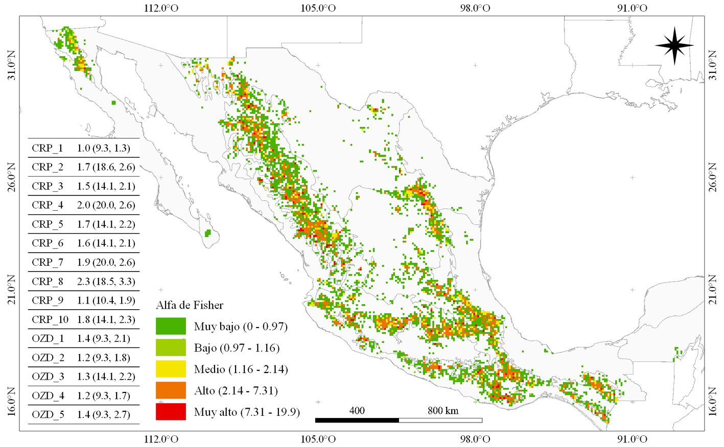
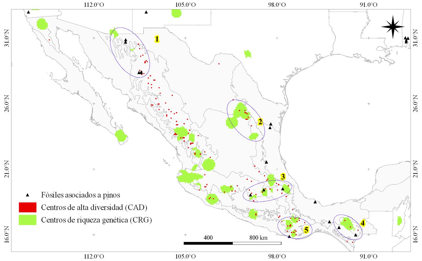
La identificación de centros de diversificación es útil para planear la conservación del germoplasma de las especies. El objetivo del estudio fue determinar las localidades que actuaron como centros de diversificación del género Pinus en México e identificar las zonas con mayor riqueza de especies de pino en la actualidad. Se construyó una base de datos de presencia (BDO) y registros fósiles (RF) para el género. A partir de ésta, se creó una malla de ~ 10 × 10 km y se determinaron centros de riqueza (CRP), centros de riqueza genética (CRG) y centros de alta diversidad (CAD) para Pinus. La coincidencia espacial de CRG, CAD y RF permitió sugerir posibles centros de diversificación de pinos (CDP). Se calculó un valor de importancia para cada CRP con base en parámetros de endemismo, rareza y riqueza de especies de pino. Se identificaron 16 CRP y 5 CDP. Los 3 CRP de mayor importancia en el país se ubican en zonas de Durango-Chihuahua (1), Coahuila-Nuevo León (2) y colindancias entre Jalisco-Zacatecas-Nayarit (3).
Palabras clave: Alta diversidad; Distribución de especies; Endemismo; Riqueza genética
Richness areas and probable diversification centers of Pinus in Mexico
Abstract
Identifying centers of diversification is useful for species germplasm conservation planning. The study objective was to determine the localities that acted as centers of diversification of the Pinus genus in Mexico and to identify current areas with the highest pine species richness. An occurrence database (BDO) and fossil records (RF) were built for the species. From this, a mesh of ~10 × 10 km was created and Centers of Pine Richness (CRP), Centers of Genetic Richness (CRG) and Centers of High Diversity (CAD) were determined. The spatial coincidence of CRG, CAD and RF allowed us to suggest possible Centers of Pine Diversification (CDP). An importance value was calculated for each CRP based on parameters of endemism, rarity, and species richness. 16 CRP and 5 CDP were identified. The 3 most important CRPs in the country are located in areas of Durango-Chihuahua (1), Coahuila-Nuevo León (2) and the boundaries between Jalisco-Zacatecas-Nayarit (3).
Keywords: High diversity; Species distribution; Endemism; Genetic richness
Introducción
El género Pinus (Pinaceae) es el grupo de coníferas más exitoso en la actualidad (Farjon, 1996), ha colonizado y domina un gran número de ambientes en el hemisferio norte, particularmente de México (Keeley, 2012; Rueda et al., 2017). Esta diversidad de pinos mexicana ha sido documentada suficientemente en revisiones generales (Farjon, 1996; Gernandt y Pérez-de la Rosa, 2014; Sáenz-Ceja et al., 2022), monografías y listados florísticos (Farjon y Filer, 2013; Sánchez-González, 2008; Villaseñor, 2016). México es también considerado un centro secundario de diversificación de Pinus (Gernandt y Pérez-de la Rosa, 2014; Millar, 1999). Sin embargo, la evidencia de la ubicación geográfica de dichos eventos es escasa.
Un centro de diversificación secundario puede entenderse como aquella región en la que un linaje ancestral dio origen a nuevas especies o nuevos linajes de especies (Millar, 1993). La identificación de centros de diversificación es útil para la conservación del germoplasma original de las especies y para estudiar los mecanismos de selección de plantas para uso humano (Fortuny-Fernández et al., 2017) y, por lo tanto, para la toma de decisiones asociadas a la planeación de acciones y políticas para la conservación y uso de la biodiversidad (Cruz-Cárdenas et al., 2013; Riemann y Exequiel, 2007). Una vez identificado el centro de diversificación de una especie o género, es relevante medir sus parámetros de riqueza y endemismo para posibilitar su monitoreo a mediano y largo plazo (Cruz-Cárdenas et al., 2013).
Existen diversas métricas para cuantificar la riqueza biológica. Algunas de uso común son los índices de riqueza, diversidad, dominancia, complementariedad, etc. Para espacios geográficos amplios se han diseñado técnicas como el análisis de punto a cuadrícula (Hijmans et al., 2012), un enfoque ampliamente aplicado al estudio de la flora mexicana (Contreras-Medina y Luna-Vega, 2007; Cruz-Cárdenas et al., 2013; Estrada-Sánchez et al., 2019; González-Espinosa et al., 2004; Ramos-Dorantes et al., 2017; Salinas-Rodríguez et al., 2018; Villaseñor et al., 2006). Sin embargo, la combinación de medidas de diversidad y el análisis de cuadrículas para predecir la riqueza y diversidad en el espacio geográfico de especies de importancia económica y ecológica, como los pinos, ha sido poco abordado en México y el mundo.
Lo descrito anteriormente destaca la importancia de comprender los aspectos históricos y biogeográficos actuales de especies de alto valor económico como los pinos. Esta investigación contribuye a responder preguntas relevantes para México como: ¿dónde se encuentran las áreas de mayor riqueza de Pinus? ¿dónde se ubican los centros probables de diversificación de Pinus? ¿cuáles son las áreas geográficas de mayor importancia para el género? todas enmarcadas en la hipótesis: ¿es posible identificar centros de diversificación del género Pinus en México, en función de la riqueza genética, alta diversidad y registros fósiles? Los objetivos del estudio fueron: identificar las áreas de mayor riqueza de Pinus, determinar las zonas más probables de diversificación de Pinus y generar un valor de importancia basado en criterios de riqueza, endemismo y rareza de pinos para las principales áreas de riqueza del género en México.
Materiales y métodos
En este estudio, la riqueza de especies se interpreta como el conteo de especies registradas en un sitio (Magurran, 1988). La riqueza genética refiere al grado de variación del material genético entre poblaciones de una especie; se consideró como centro de riqueza genética aquellas regiones donde se concentra la mayor cantidad de poblaciones, asumiendo que las regiones con mayor número de poblaciones serán genéticamente más diversas (Conabio, 2007). Los centros de alta diversidad se entienden como aquellos sitios con valores altos de un índice de diversidad biológica. El concepto de endemismo se aplica como un indicador de restricción en la distribución geográfica de las especies.
La figura 1 esquematiza el flujo de trabajo realizado para alcanzar los objetivos del presente estudio. Los párrafos precedentes detallan los procedimientos realizados en cada una de las etapas del análisis.
Se construyó una base de registros fósiles y datos de presencia (BDO) de especies de Pinus que se distribuyen de forma natural en México. Se consultaron fuentes de datos especializadas como Global Biodiversity Information Facility (www.gbif.org/), Sistema Nacional de Información sobre Biodiversidad de México (www.snib.mx/), Red Mundial sobre Información sobre Biodiversidad (http://www.conabio.gob.mx), SEINet (www.swbiodiversity.org) y revisión de literatura científica mediante motores de búsqueda web (e.g., Google Scholar, Springer, Scopus; con juegos de palabras: “especie”, “latitud”, “longitud”, “coordenadas”, “Pinus”, “México”) en idioma español e inglés.
Posteriormente, se depuró la BDO eliminando datos sin coordenadas, mal georreferenciados y duplicados (de una especie) en pixeles de 1 km2. Se consideraron como válidas las entidades taxonómicas definidas en publicaciones recientes (Buck et al., 2020, 2023; Farjon, 2018; Montes et al., 2019, 2022; Pérez-de la Rosa & Gernandt, 2017; Willyard et al., 2017, 2021) y se consultaron sitios especializados (http://www.worldfloraonline.org/, https://powo.science.kew.org/) para asignar nombres intraespecíficos a cada especie. Adicionalmente, la BDO se filtró con base en el rango altitudinal reportado en la literatura para cada especie de Pinus (Farjon, 2017; Farjon y Filer, 2013), excluyendo datos cuando la combinación ambiental de esos sitios se ubicó fuera de la combinación de los mismos factores para el rango altitudinal reportado en la literatura (material suplementario: fig. S1).
Figura 1. Esquema de trabajo seguido para la identificación de centros de alta diversidad, riqueza genética y posibles centros de diversificación del género Pinus en México. Información inicial (azul), procesos y algoritmos (verde), principales configuraciones de procesos y algoritmos (naranja y morado) y productos generados (bordes redondos) durante este estudio. Los principales objetivos de la investigación se muestran con borde segmentado. Tamaño de pixel de ~ 10 x 10 km con: tipo de vecindad simple (*) y circular de un grado sexagesimal (§).
A partir de la BDO, inicialmente se realizó un análisis de “Point to grid/ Richness/ Number of different classes” con vecindad simple (~ 10 × 10 km) en el programa DIVA-GIS v. 7.5.0 (Hijmans et al., 2012), asignando a cada pixel el número de especies contabilizado dentro del mismo, lo cual constituyó la riqueza observada. Posteriormente, se identificaron y seleccionaron conglomerados de pixeles contiguos a los que se llamó centros de riqueza de pinos (CRP). Considerando que la BDO no proviene de un muestreo geográficamente uniforme, se observaron otros grupos de pixeles no contiguos donde se presentaron valores importantes de riqueza. Tales conjuntos se agruparon y se nombraron como otras zonas dispersas de riqueza de pinos (OZD). La delimitación de los CRP y OZD se realizó de forma manual mediante un sistema de información geográfica (Quantum GIS Team Development, 2019) y se numeraron de forma consecutiva solo con propósito de identificación —no representa valor de importancia. Para identificar de forma puntual pixeles de mayor riqueza, los datos de riqueza observada a nivel pixel se clasificaron en 5 estratos mediante el método de intervalos geométricos (1 = muy baja, 2 = baja, 3 = media, 4 = alta y 5 = muy alta). Los pixeles pertenecientes al estrato superior (5 = muy alta) fueron considerados los sitios con mayor riqueza de especies de pinos dentro de los CRP y OZD (fig. 2). De acuerdo con Arenas-Navarro et al. (2020), se calculó el cociente (Es) entre la riqueza observada y la riqueza estimada (estimador no paramétrico de Chao2) por pixel, como un indicador de la calidad de las celdas resultantes del análisis de punto a cuadrícula. Los estimadores no paramétricos (e.g., Chao2) tienen la particularidad de ser menos sesgados que los de tipo paramétrico (Brose et al., 2003).
Partiendo de la BDO, mediante el módulo “Point to grid/ Richness/ Number of observations” de DIVA-GIS (Hijmans et al., 2012), se realizó un análisis punto a cuadrícula para delimitar, a nivel especie, las zonas geográficas con mayor número de presencias, lo que se tradujo en zonas de mayor riqueza genética a nivel especie (Conabio, 2007; fig. 3A-D). Para ello, se utilizó una resolución espacial (tamaño de pixel) de 0.083 grados sexagesimales (~ 10 × 10 km). Para cada especie analizada, el procedimiento generó 5 estratos (intervalo igual) de abundancia de registros de presencia (fig. 3A, B). Se nombró como centro de riqueza genética (CRG) solo al estrato superior (fig. 3C), el cual se convirtió a formato binario (1 = CRG; 0 = área sin interés; fig. 3D). De esta forma se delimitó el CRG para cada especie incluida en la BDO. Finalmente, los CRG a nivel especie se sobrepusieron espacialmente para determinar los CRG a nivel género en México.
Se utilizó el índice alfa de Fisher para estimar la diversidad de especies de Pinus a nivel pixel (~ 10 × 10 km) (Fisher et al., 1943). A pesar de que alfa de Fisher (α) es poco utilizado actualmente, decidimos utilizarlo por 2 razones: no se dispuso de datos de densidad de las especies de pino a nivel localidad y a diferencia de otros índices como Shannon-Wiener, Simpson, Margalef, Menhinick, entre otros, de uso común para propósitos similares, α es poco sensible al número de individuos muestreados, a la presencia de especies raras o comunes y al tamaño del área estudiada (Magurran, 1988). Adicionalmente, a excepción de α, los índices antes mencionados son adecuados para medir la heterogeneidad de especies localmente (Peet, 1974), por lo que al manejar unidades de estudio de gran tamaño (pixel de 10 × 10 km) en este estudio, consideramos que α es el índice más adecuado para los propósitos planteados.
Las estimaciones de α a nivel pixel se realizaron mediante el programa PAST v. 4.03 (Hammer et al., 2001). Posteriormente, mediante el método de reclasificación de intervalos geométricos se definieron 5 estratos de las predicciones de α (1 = muy baja, 2 = baja, 3 = media, 4 = alta y 5 = muy alta diversidad), de los cuales solo se retuvo el estrato superior y se convirtió a formato binario para representar los centros de alta diversidad (CAD) de Pinus en México.
Los posibles CDP en México se identificaron como aquellas áreas de coincidencia espacial (intersección) entre los CRG (nivel género) y los CAD (Santillán-Fernández et al., 2021), además de la presencia cercana a estas áreas de fósiles de Pinus. Partimos del supuesto que el registro fósil en áreas de alta riqueza del género Pinus, o cerca de éstas, indica la presencia del género Pinus desde épocas ancestrales.
Se generó un valor de importancia para cada área de riqueza en función de 4 criterios: I) valor promedio de endemismo, II) número de especies que se distribuyen en el área, III) número de especies raras y IV) riqueza máxima de especies por pixel (~ 10 × 10 km). El indicador I se obtuvo utilizando el método propuesto por Kerr (1997), que es la sumatoria del inverso al número de pixeles donde aparece cada especie, obteniendo el valor final mediante el promedio de todos los pixeles del área. Este método ha sido aplicado para identificar zonas de endemismo de plantas mexicanas (Estrada-Sánchez et al., 2019; Riemann y Exequiel, 2007; Villaseñor et al., 2006). Para el indicador III, se utilizó el índice de rareza propuesto por Maciel (2021), el cual genera un valor en función del rango geográfico, especificidad de hábitat y abundancia (número de presencias de la especie por pixel, en este trabajo) de la especie (Maciel, 2021). Se utilizó la mediana del índice de rareza para definir especies raras y comunes (material suplementario: tabla S1). Para estimar los indicadores II y IV, se contó el número de taxones distribuidos en el área y el número máximo de ellos en un pixel, respectivamente. Finalmente, los criterios I, II, III y IV fueron normalizados a valores en intervalo de 0 a 1 (para cada puntaje obtenido se restó valor mínimo de ese criterio y ésto se dividió entre la diferencia del máximo y el mínimo del mismo criterio) y se sumaron para obtener un valor final de importancia para cada CRP y OZD.
Resultados
Se consideraron como válidas 48 especies del género Pinus (material suplementario: tabla S1) que se distribuyen de manera total o parcial en México. El número de registros que integraron la BDO después del proceso de limpieza fue de 32,030 (un registro por especie dentro de 1 km2), de los cuales solo 64.6% (20,709) se ubican dentro del territorio mexicano. Las fuentes que aportaron mayor cantidad de datos a la base final fueron GBIF (67.1%), SEINet (12.4%), SNIB (8.5%), literatura científica (7.1%) y un porcentaje menor para otras fuentes. Así mismo, 18.8% de las 48 especies tuvo más de 1,000 registros, 60.4% entre 100 a 1,000 registros, 6.3% entre 50 y 99, y 14.6% menos de 50 registros. La especie con más registros fue P. leiophylla (3,555 registros) y la de menos P. vallartensis (9 registros), una especie descrita recientemente en el occidente de México. El 24.3% de las presencias se registró antes de 1980, 24% entre 1981 y 2000, y el restante 58.1% entre 2001 y mediados de 2022.
El promedio del indicador de calidad de celdas en cada CRP y OZD varió entre 0.87 y 0.98 (material suplementario: tabla S1). Los valores de riqueza por pixel variaron entre 1 y 13 (fig. 2A). Las clases alta y muy alta de riqueza observada se restringieron a zonas concretas de la sierra Madre Occidental (SMOc), sierra Madre Oriental (SMOr), sierra Madre del Sur (SMS) y sierras de Chiapas (fig. 2Aa). Los pixeles con menor riqueza observada se registraron principalmente en la periferia de los relieves antes mencionados (fig. 2A). El estrato de muy alta riqueza (estrato 5 de riqueza observada; fig. 2Aa) va de 6 a 13 especies y se ubicaron de forma muy dispersa en algunas zonas de Durango, Chihuahua, Nuevo León, Jalisco, Michoacán, México, Guerrero, Oaxaca y Chiapas (pixeles rojos, fig. 2B).
Figura 2. Riqueza observada (A), riqueza observada estratificada (Aa) y áreas de riqueza de especies de Pinus (B) en México. En la simbología de B, el número en paréntesis indica el número de especies presentes en el área definida. Por ejemplo, CRP_1 (9) indica que en el área CRP_1 se registró la presencia de 9 especies; no indica que 9 especies fueron observadas en cada pixel (~ 10 x 10 km) del área. Las líneas que dividen el interior de México corresponden a los límites de las regiones biogeográficas contenidas.
El análisis de punto a cuadrícula detectó 10 conglomerados de CRP y 6 de OZD (fig. 2B). Es importante reiterar que el número de especies mencionados en este párrafo —número entre paréntesis en la fig. 2B— no indican que tal número se observó en cada pixel que forma parte del CRP u OZD, sino que se identificó al menos un registro de cada especie en algún pixel de dicha zona. En las áreas compactas, el mayor número de especies fue 21 (CRP_2) y el menor fue 9 (CRP_1; Baja California). En la SMOc se ubicó el área de riqueza de mayor tamaño (CRP_2), mientras que en la porción michoacana de la SMS se ubicó la de menor extensión (OZD_5). En la zona centro-oriental de la FVT se identificaron 3 áreas (CRP_4, 5, 6), cuyo número de especies aumenta de 15 en la zona este a 17 en la zona oeste. En la zona media de la SMOr se identificó un área compacta (CRP_3) y 2 áreas dispersas (OZD_4 y OZD_6) en los extremos sur y norte, respectivamente. Las OZD figuran en la periferia de las áreas compactas (fig. 2B).
Las zonas dispersas (OZD) que contaron con alto número de especies fueron el oeste de la FVT (OZD_3; sur de Zacatecas, Jalisco y Nayarit; 21 especies) y el sur de la SMOr (18 especies, Querétaro, San Luis Potosí; OZD_4), mientras que la sierra sur de Michoacán (OZD_5) fue el área de pixeles dispersos con menor presencia de especies de pino (8 especies). Finalmente, algunas áreas como CRP_1, CRP_9, OZD_2 y OZD_4 tuvieron nula o muy poca presencia de pixeles de muy alta riqueza de pinos (fig. 2B).
La delimitación de la zona de mayor concentración de presencia para cada taxón en la BDO identificó el CRG para cada especie (fig. 3A-D). Los CRG identificados representan áreas pequeñas dispersas en el territorio, ubicadas principalmente en la zona sur de la SMOc y este de la FVT, la zona media de la SMOr (Coahuila y Nuevo León) y algunas áreas en las zonas montañosas de Oaxaca y Chiapas (fig. 3E-G). En algunas zonas geográficas se observaron coincidencias del CRG para más de 1 especie, siendo las más notables en el sureste de Durango (fig. 3E-G), en colindancias entre Coahuila y Nuevo León (fig. 3F) y en Chiapas (fig. 3E-G). Para las especies con presencia periférica en México (e.g., Pinus coulteri y P. lambertiana) los CRG se detectaron fuera del territorio mexicano. Por otro lado, aunque no fueron coincidentes espacialmente, estados como Oaxaca, Jalisco, Durango y Michoacán mostraron CRG para más de 1 especie. De manera contraria, aunque se presentan 9 especies en el CRP_1, solo se observó el CRG para P. quadrifolia y P. jeffreyi al igual que para el OZD_5 que únicamente representó el CRG para P. rzedowskii (fig. 3F).
Figura 3. Ejemplo de la determinación del centro de riqueza genética (CRG) para Pinuspatula (A-D) y centro de riqueza genética para especies de la subsección Australes (E), Cembroides y Nelsoniae (F), Ponderosae y Strobus (G) y a nivel género (H). Las líneas que dividen el interior de México corresponden a los límites de las regiones biogeográficas contenidas.
La distribución espacial del estrato superior (estrato 5 = muy alta diversidad) de α, definido como CAD, se ubicó principalmente en zonas de la SMOc, SMOr, FVT, además de algunas secciones de la SMS y muy poca presencia en los macizos montañosos de Chiapas. De manera más puntual, la mayor cantidad de pixeles de CAD se observó en la FVT, Chihuahua, Durango y Oaxaca, otros pixeles más aislados se identificaron entre Coahuila y Nuevo León, Guerrero y Chiapas (fig. 4).
El cálculo del índice alfa de Fisher (α) por pixel mostró diferencias importantes por zona geográfica. Los valores más altos se observaron en zonas particulares de los sistemas montañosos más importantes de México (fig. 4). Los estados de Chihuahua, Durango, Nuevo León, Michoacán, Oaxaca y algunas zonas de la FVT presentaron pixeles con los valores más altos de α (fig.4). En los CRP y OZD, el promedio de α varió de 0.9 (OZD_6) a 2.3 (CRP_8). El valor máximo por pixel, α = 20, se encontró para los CRP_7 (sierra norte de Oaxaca) y CRP_4 (Michoacán), aunque Chihuahua y Durango (CRP_2) y la sierra sur de Oaxaca (CRP_8) también exhibieron valores máximos altos (α = 18.6) por pixel. Por el contrario, el valor máximo de menor magnitud de α por pixel dentro de un CRP u OZD fue de 9.3 (Baja California, Guerrero, Chiapas, San Luis Potosí y Querétaro; fig. 4). La menor variabilidad (segundo valor del paréntesis en tabla de la fig. 4) en las predicciones de α se presentó para el CRP_1 (Baja California), mientras para el CRP_8 (sierra sur de Oaxaca) se observó lo contrario.
La coincidencia espacial (intersección) de los centros de alta diversidad (CAD) y los centros de riqueza genética (CRG) de los pinos mexicanos fue evidente en algunas zonas de los principales sistemas montañosos de México (fig. 5). Lo anterior, conjuntamente con los registros de fósiles de Pinus encontrados en México, permitió la identificación de áreas que, argumentamos, tienen una alta probabilidad de haber sido centros de diversificación para Pinus en el pasado. Entre estas áreas destaca el extremo norte de la SMOc (Chihuahua y Sonora; 1), la zona media de la SMOr (sur de Coahuila, Nuevo León y Tamaulipas; 2), el centro-este de la FVT (3) y otras zonas sureñas como los macizos montañosos de Chiapas (4) y la sierra sur de Oaxaca (5). Para áreas como Baja California, sur de SMOc y oeste de la FVT no se encontró material fósil (fig. 5), aunque para las 2 últimas existe una alta coincidencia entre CAD y CRG de pinos.
Zonas de mayor importancia para Pinus en México
El cálculo de endemismo, riqueza de especies, rareza y riqueza máxima por pixel, posibilitó la asignación de un valor de importancia para cada CRP y OZD. El área ubicada en la zona media de la SMOc (CRP_2; Durango y Chihuahua) presentó el mayor número de especies (21) y riqueza máxima (13), por lo que obtuvo también el mayor valor de importancia, 3.471 (tabla 1). En orden decreciente, siguieron la zona intermedia de la SMOr (CRP_3) y la zona ubicada en el este de la FVT (OZD_3). El CRP_3 obtuvo el segundo valor más alto en los criterios de endemismo (tabla 1) y la OZD_3 presentó el mayor número de especies raras y el número máximo de especies presentes (21). El valor de importancia para dichas áreas fue 3.056 (CRP_3) y 2.601 (OZD_3).
Algunas zonas con valores medios de importancia son el CRP_4, CRP_7 y OZD_4, los cuales presentaron niveles intermedios de riqueza máxima (12, 12 y 9 especies, respectivamente) y especies raras (5 en promedio; tabla 1). Las áreas que presentaron los valores más bajos de importancia fueron las ubicadas en la sierra sur de Michoacán (OZD_5; 0.287), el noroeste de México (CRP_1; 0.635) y el sistema montañoso costero de Chiapas (OZD_2; 0.661; tabla 1). De forma general, se observaron 7 áreas (resaltadas con negritas en tabla 1) con un valor final por arriba del promedio (1.718), las cuales podrían considerarse como las áreas de mayor importancia de Pinus en México, basándose en criterios de endemismo, rareza y riqueza.
Discusión
La delimitación de los CRP tuvo como objetivo señalar las áreas de mayor riqueza de Pinus en México. Con base en las ecorregiones de Olson et al. (2001), se observó que a lo largo de la FVT existen intervenciones de bosques secos pertenecientes a la Depresión del Balsas, similar a los que separan los macizos montañosos de Chiapas (OZD_2 y CRP_10). En el sur de San Luis Potosí (SMOr), los matorrales de la meseta central y los bosques húmedos de Veracruz interrumpen la continuidad de los bosques de pino-encino. La baja presencia de celdas con presencia de pinos en estas zonas, condujo a la delimitación de los CRP y OZD expuestos en este estudio. Además, para la SMS la regionalización basada en criterios biológicos y climáticos propuesta por Morrone (2019), muestra zonas fragmentadas cuya disposición geográfica coincide parcialmente con los CRP_7, 8, 9 y OZD_1. De forma similar, la zonificación de Suárez-Mota et al. (2013) para la FVT se asemeja geográficamente a la OZD_3 y CRP_6, mientras que los centros críticos de riqueza para musgos y senecios señalados por Villaseñor et al. (2006), coinciden geográficamente con los CRP y OZD identificados para la FVT.
Figura 4. Índice alfa de Fisher (α) para especies de Pinus en México. La tabla muestra el valor promedio (máximo, desviación estándar) por pixel de α en las áreas de riqueza de especies (CRP, OZD) definidas previamente. Tamaño de pixel ~ 10 x 10 km.
Figura 5. Centros de riqueza genética (CRG), alta diversidad (CAD) y posibles centros de diversificación (indicados con elipses y números resaltados en color amarillo) de Pinus en México —las elipses y su numeración se presentan solo con fines de visualización. Las líneas que dividen el interior de México corresponden a los límites de las regiones biogeográficas contenidas.
Se identificó un número mayor de áreas de riqueza de Pinus con respecto a estudios previos (Farjon, 1996; Sáenz-Ceja et al., 2022; Sánchez-González, 2008). Esto podría explicarse por lo siguiente: 1) el propósito de este estudio fue identificar las zonas con mayor riqueza y no el patrón general de distribución del género en México; 2) los CRP fueron identificados a partir de coordenadas provenientes de colecciones biológicas y estudios científicos, lo que no garantiza su distribución geográfica uniforme y deriva en la identificación de zonas fragmentadas y de menor tamaño y 3) diferencias metodológicas (e.g., análisis de punto a cuadrícula y modelos de distribución potencial) en la determinación de las áreas de riqueza. En relación con el número de especies, también se presentaron diferencias importantes con estudios previos. Por ejemplo, para el noroeste de México (CRP_1), se han mencionado 9, 10 y 19 especies (Farjon, 1996; Sáenz-Ceja et al., 2022; Sánchez-González, 2008, respectivamente), siendo la primera y segunda similares a las 9 registradas aquí (fig. 2B), pero con diferencias en las entidades taxonómicas. Tales variaciones pueden deberse a: 1) metodología: solo se contabilizaron las especies dentro de los pixeles incluidos en CRP_1 y no para toda la península, por lo que especies como P. lagunae (Rob-Pass.) Passini no están incluidas en la cifra mencionada (9 especies); 2) taxonomía: el nivel taxonómico empleado fue especie, con base en las entidades reconocidas por Farjon (2018) y estudios recientes sobre delimitacion de especies (Buck et al., 2020, 2023; Montes et al., 2019, 2022; Willyard et al., 2017, 2021). El número de especies observado (9, 21, 17, 16) en algunas regiones como CRP_1, 2, 3 y 7 es cercano a las 7, 20, 14 y 15 mencionadas por Sáenz-Ceja et al. (2022) respectivamente, en zonas coincidentes con las áreas de riqueza mencionadas.
Tabla 1
Valores de los criterios considerados para la asignación de un valor de importancia (V.I.) para centros de riqueza de especies de Pinus (CRP) en México. En negritas se indican los 7 CRP identificados como más importantes.
CRP
Pixeles
E* (I)
S (II)
Sr§ (III)
Rm (IV)
V.I.
CRP_1
164
0.309 (0.021)
0.077 (9)
0.250 (4)
0.000 (5)
0.636 (15)
CRP_2
1212
0.596 (0.031)
1.000 (21)
0.875 (9)
1.000 (13)
3.471 (1)
CRP_3
280
0.739 (0.036)
0.692 (17)
0.875 (9)
0.750 (11)
3.056 (2)
CRP_4
164
0.300 (0.021)
0.692 (17)
0.375 (5)
0.875 (12)
2.242 (4)
CRP_5
274
0.349 (0.022)
0.615 (16)
0.250 (4)
0.625 (10)
1.840 (7)
CRP_6
299
0.348 (0.022)
0.538 (15)
0.250 (4)
0.375 (8)
1.511 (10)
CRP_7
159
0.366 (0.023)
0.615 (16)
0.250 (4)
0.875 (12)
2.106 (5)
CRP_8
136
0.187 (0.017)
0.615 (16)
0.250 (4)
0.500 (9)
1.552 (9)
CRP_9
133
0.000 (0.010)
0.462 (14)
0.250 (4)
0.250 (7)
0.962 (13)
CRP_10
107
0.404 (0.024)
0.308 (12)
0.000 (2)
0.750 (11)
1.461 (11)
OZD_1
112
0.205 (0.017)
0.538 (15)
0.250 (4)
0.375 (8)
1.369 (12)
OZD_2
107
0.132 (0.015)
0.154 (10)
0.000 (2)
0.375 (8)
0.660 (14)
OZD_3
345
0.101 (0.014)
1.000 (21)
1.000 (10)
0.500 (9)
2.601 (3)
OZD_4
164
0.274 (0.020)
0.769 (18)
0.500 (6)
0.500 (9)
2.043 (6)
OZD_5
38
0.038 (0.011)
0.000 (8)
0.000 (2)
0.250 (7)
0.288 (16)
OZD_6
89
1.000 (0.046)
0.077 (9)
0.500 (6)
0.125 (6)
1.702 (8)
E = Endemismo; S = número de especies; Sr = número de especies raras; Rm = riqueza máxima por pixel; V.I. = valor de importancia (el valor entre paréntesis representa el orden de importancia); * = promedio del valor de endemismo por pixel obtenido mediante el índice de endemismo propuesto por Kerr (1997); § = la determinación de una especies rara o común se realizó con base en el índice de rareza propuesto por Maciel (2021). El orden de los valores de I a IV es el valor obtenido por la normalización del criterio (valor neto obtenido del criterio).
Algunos estudios a nivel local, como el de Ramos-Dorantes et al. (2017) mencionaron 16 especies (Puebla; CRP_6), mientras que 15 fueron las registradas en este trabajo. En inventarios florísticos de áreas naturales protegidas (ANP) como la Reserva de la Biosfera Mariposa Monarca (CRP_5), Reserva Forestal Nacional y Zona de Refugio de la Fauna Silvestre Tutuaca (CRP_2), se han reportado 15 y 12 especies, que es cercano a los observado (16 y 12) en tales sitios. Así mismo, en la Reserva de la Biosfera La Sepultura (OZD_2) y la Reserva de la Biosfera Sierra Gorda (OZD_4) se mencionan 10 y 3 especies de pino, mientras que en este estudio se registraron cifras superiores (13 y 6, respectivamente). Tales discrepancias en número de especies pueden ser posibles debido a que una especie podría presentarse dentro del CRP y estar ausente dentro de la ANP. Las ANP son espacios destinados a la conservación debido a su elevada riqueza biológica (Salinas-Rodríguez et al., 2018), por lo que se considera que pueden ser un contraste adecuado para el número de especies registrado en este estudio.
Estudios locales como el de Ríos-Altamirano et al. (2016) y Martin et al. (2021) en Oaxaca (CRP_7) describen 10 y 7 especies, respectivamente; mientras que en los pixeles que abarcan tales sitios se registraron 13 y 8 especies. En el CRP_2 (SMOc), González-Elizondo et al. (2012) mencionaron 20 especies, mientras que en este trabajo se observaron 21. Lo anterior demuestra que BDO construida y los análisis subsecuentes, son una adecuada representación de la riqueza de los pinos en México.
El aporte fundamental de los resultados de este trabajo es que puede considerarse una actualización de revisiones históricas sobre la biogeografía de Pinus (a nivel especie) en México y además, señalan de forma concreta áreas con alta riqueza, excluyendo áreas con baja o nula presencia. Sin embargo, es importante considerar que, como en cualquier análisis, los resultados dependen de los datos utilizados. Esto es relevante considerando que, recientemente, se han ventilado limitaciones y sesgos espaciales, temporales y filogenéticos de las bases digitales de registros de presencia de plantas vasculares, particularmente de la base GBIF utilizada en este trabajo (Ramírez-Barahona et al., 2023), con un aporte mayoritario de los registros de aparición (60% de total). Afortunadamente, de acuerdo con estos autores, algunas zonas montañosas de México, como aquellas que asemejan el patrón de presencia de Pinus en el país (SMOr, SMOc, FVT, SMS), son zonas con bajo sesgo espacial y temporal de recolectas de plantas vasculares (ver. fig. S4 en Ramírez-Barahona et al. [2023]). Por otro lado, en los análisis se incorporaron registros de aparición de otras fuentes (40% de los registros), lo que sin duda contribuye a disminuir los sesgos inherentes de los datos de GBIF. Además, la cercanía al valor óptimo (Es = 1) de las estimaciones sobre la calidad de las celdas (Es = 0.88 a 0.98) que formaron las áreas de riqueza de pinos identificadas aquí, sugiere una calidad suficiente para el alcance de los objetivos de este estudio (Arenas-Navarro et al., 2020).
El enfoque empleado para determinar los CRG ha sido empleado para delimitar la riqueza genética de razas de maíz en México y se desconoce su utilización en árboles (Santillán-Fernández et al., 2021). Sin embargo, existen datos que de manera indirecta podrían indicar alguna relación con los CRG identificados en este estudio. Por ejemplo, para P. greggii, Parraguirre-Lezama et al. (2002) reportaron menor número de alelos y porcentaje de polimorfismo en las poblaciones del sur (Hidalgo y Querétaro) con respecto a las del norte (Coahuila y Nuevo León), estas últimas se encuentran dentro del CRG señalado para esta especie (fig. 3E). Así mismo, García-Gómez et al. (2014) estudiaron 4 poblaciones de P. johannis y encontraron mayor número de loci polimórficos en una población (Salaverna, Zacatecas) que coincide espacialmente con el CRG identificado para esta especie (fig. 3F). El polimorfismo genético, la heterocigocidad esperada y observada, y el número de alelos, son usados para denotar diferencias en el acervo genético entre poblaciones de una especie (García-Gomez et al., 2014; González-Jiménez et al., 2021; Ledig et al., 2001).
De igual manera, poblaciones con altos valores de heterocigocidad esperada y riqueza alélica de P. remota (González-Jiménez et al., 2021) y P. pinceana (Ledig et al., 2001) coinciden espacialmente con los CRG para ambas especies (Coahuila y Nuevo León), aunque los 2 estudios citados anteriormente no han tomado en cuenta el rango completo de distribución de la especie. La evidencia anterior sugiere coincidencia geográfica entre los CRG delimitados espacialmente y la diversidad genética a nivel población, aunque se necesita mayor investigación para reforzar estos hallazgos, sobre todo con especies de amplia distribución, las cuales representan al menos 50% de este estudio.
Los valores más altos de α se ubicaron principalmente en la SMOc (Durango y Chihuahua), SMOr (Coahuila y Nuevo León), en el centro-este de la FVT y macizos montañosos de Oaxaca y Chiapas (fig. 4), emulando el patrón general de distribución del género (Rzedowski, 2006; Sáenz-Ceja et al., 2022). Aunque no existen estimaciones de α en pixeles espaciales de gran tamaño (e.g. 10 × 10 km ), sí existen estimaciones en ecosistemas con presencia de pinos, pero no exclusivamente para éstos.
En bosques mixtos de pino-encino en Oaxaca (CRP_9), Aguilar-Santelises y Castillo (2013) reportaron un α de 4.55, mientras que en rodales de la misma entidad con y sin manejo silvícola (CRP_7), Luna-Bautista et al. (2015) encontraron valores promedio de 1.778. En el sur de México (Chiapas; CRP_10), Cayuela et al. (2006) estimaron α máximo de 10.6 para rodales de pino-encino. Sánchez-González y López-Mata (2005) describen promedios de 1.01 de α en un gradiente altitudinal (bosque de encino, mixto, pino-pastizales alpinos) perteneciente al CRP_5 (este del Estado de México). En las ubicaciones de los estudios mencionados anteriormente, nuestro α fue mayor al reportado por los autores: α = 5.453, 6.376, 14.1 y 2.86 en el mismo orden. El resultado de este contraste es opuesto a lo esperado, ya que los análisis en comparación incluyeron diversos géneros de plantas (e.g. Juniperus, Arbutus, Quercus, Prunus y Alnus) y, por lo tanto, un mayor recuento de especies a nivel de sitio, lo que debería resultar en un valor mayor de α. Lo anterior podría deberse a las diferencias en el tamaño del sitio analizado. Este estudio tuvo como base de análisis pixeles de ~ 10 × 10 km, lo que posibilitó que en un pixel pudieran observarse más especies y más presencias (aunque no de la misma localidad). Contrariamente, el área muestreada en los otros estudios varió de parcelas de 400 m2 a 1,000 m2 (Cayuela et al., 2006; Luna-Bautista et al., 2015; Sánchez-González y López-Mata, 2005).
El hecho de que los CRP hayan tendido un bajo promedio de α (comparado con el máximo) pudo deberse a la distribución geográfica heterogénea de los registros presencia, que refleja un bajo esfuerzo de muestreo, sobre todo en la periferia de los CRP y OZD. A pesar de lo anterior, los valores obtenidos sobre la calidad de las celdas fueron cercanos al óptimo (material suplementario: tabla S1), por lo que puede considerarse que las celdas (al menos dentro de los CRP y OZD) tuvieron la calidad suficiente para el alcance de los objetivos de este estudio. Además, aunque es evidente que existen importantes deficiencias en la información disponible sobre biodiversidad (Ramírez-Barahona et al., 2023), las colecciones biológicas son la principal fuente de información en estudios de diversidad (Arenas-Navarro et al., 2020; Ramos-Dorantes et al., 2017; Salinas-Rodríguez et al., 2018; Suárez-Mota et al., 2018). Sin embargo, es importante enfatizar que a medida que avance la recolecta y digitalización de información biológica del país, se podrán refinar las estimaciones de diversidad de pinos en sus diversas áreas de riqueza. La información biológica sobre riqueza y diversidad es fundamental para el diseño de políticas que aseguren la permanencia de especies (Riemann y Exequiel, 2007), sobre todo aquellas con alto valor económico y ecológico como los pinos.
Posterior a su origen, el género Pinus experimentó ciclos de expansión y retroceso acoplados a fluctuaciones climáticas (Millar, 1993, 1999; Stults et al., 2010). Durante este periodo, la competencia con angiospermas (Millar, 1993), la interacción y efecto del fuego (Jin et al., 2021; Keeley, 2012), estrés por sequía y tolerancia a la sombra (Rueda et al., 2017) impulsaron su ruta evolutiva. Los probables CDP en México, identificados en este estudio por la intersección de CRG, CAD y registros fósiles, aproximan la ubicación de áreas que probablemente potenciaron la amplia distribución actual del género (Farjon, 1996; Millar, 1993). Los autores desconocen la existencia de estudios específicos sobre áreas con alta probabilidad de presencia de fenómenos de diversificación de Pinus en el pasado, por tanto, estos resultados representan un aporte importante que coadyuva al entendimiento del fenómeno.
Algunos autores nombran como “centros secundarios de origen” a zonas de latitud media con alta diversidad dentro del género (Millar, 1999), siendo en épocas recientes (Mioceno, ~ 5 – 22.5 Ma) cuando se originó su diversidad actual (Farjon, 1996; Jin et al., 2021). Aunque los fósiles hallados en tierras bajas de Chiapas que datan de al menos 90 Ma (Huerta-Vergara et al., 2013) indicarían que tales regiones ya eran habitadas por pinos antiguos mucho antes de la reciente historia evolutiva del género. De acuerdo con Jin et al. (2021), la tasa neta de diversificación de Pinus ha decrecido considerablemente desde finales del Cretácico (~ 100 Ma), por lo que, de haber existido linajes de pinos en regiones como el México antiguo, su diversidad pudo haber sido más amplia que la actual. Esto último sigue siendo una incógnita puesto que el siguiente hallazgo fósil para México, encontrado en tierras bajas de Veracruz (Millar, 1993) data de mediados del Mioceno (~ 15 Ma), justo antes del inicio de la gran radiación actual de Pinus en esta región.
Sea como centro de diversificación o centro secundario de origen, México ha sido importante en la evolución de Pinus. Las altas tasas de diversificación del género en el país fueron desencadenadas por la actividad volcánica del Paleógeno (entre 60 y 37 Ma) (Farjon, 1996). El constante levantamiento de las principales cordilleras generó diferencias altitudinales, amplia variabilidad de suelos y una paulatina aridez con la formación del altiplano mexicano, que en épocas posteriores actuó como barrera geográfica entre zonas habitables para pinos (Millar, 1993). La heterogeneidad ambiental y el aislamiento propiciaron fragmentación, divergencia y especiación de los pinos en esas épocas (Millar, 1999; Stults et al., 2010). Además, una caída abrupta de temperatura en épocas subsecuentes ocasionó la retirada de las angiospermas hacia los trópicos (Millar, 1993), lo cual fue clave para que Pinus se expandiera a menores latitudes (Keeley, 2012). En conjunto, un clima frío, disminución de competencia y una amplia variabilidad ambiental pudieron haber provocado la liberación de una cantidad importante de nichos, lo cuales fueron ocupados por los ancestros de los pinos actuales. Esto último puede respaldarse en los hallazgos de Jin et al. (2021), quienes mencionan que la evolución del nicho ecológico y variaciones fenotípicas en Pinus aumentaron considerablemente a inicios del Oligoceno (que es la época subsecuente al gran enfriamiento mencionado anteriormente).
Zonas de importancia para Pinus en México.
El alto valor de importancia para el CRP_2 (SMOc) es explicado por presentar el máximo valor en riqueza (21 especies) y riqueza máxima (13 especies por pixel), el segundo valor más alto por especies raras y el tercer valor más alto por endemismo. Tales valores de endemismo, rareza y riqueza (tabla 1) contribuyeron a clasificarlo como el CRP de mayor importancia en México. Para algunos taxones, este CRP representa la latitud máxima (e.g., P. teocote, P. oocarpa y P. pseudostrobus), mínima (P. brachyptera) y una zona de continuidad para otras (P. strobiformis, P. arizonica y P. leiophylla), además, alberga una de las 2 poblaciones conocidas de P. maximartinezii (González-Elizondo et al., 2011). En el contexto anterior, González-Elizondo et al. (2012) mencionan que Pinus es uno de los 3 géneros más abundantes de la SMOc (24 especies). Además, los bosques del CRP_2 representan una de las zonas con mayor aporte económico al sector forestal del país (Hernández-Salas et al., 2013), lo cual hace aún más evidente la importancia tanto ecológica como económica de esta área. La zona media de la SMOc (Chihuahua y Durango) representa una de las zonas de mayor prioridad para la conservación de Pinus en México (Sáenz-Ceja et al., 2022).
Se ha sugerido que la SMOr se originó hace ~ 65 Ma, aunque se han encontrado fósiles de pinos más antiguos en el sur de México (~ 90 Ma; Chiapas; Huerta-Vergara et al., 2013), por lo que durante su emergencia y las fuertes fluctuaciones climáticas subsecuentes (Millar, 1993, 1999), la SMOr pudo haber sido un refugio para los linajes de Pinus existentes y otros grupos de plantas (Salinas-Rodríguez et al., 2017), incluso atribuyéndosele el origen de la subsección Cembroides (Farjon, 1996). Lo anterior explicaría el alto valor de importancia para CRP_3 (tabla 1), además de la presencia de especies endémicas (P. nelsonii y P. culminicola) y de distribución restringida (P. remota, P. pinceana y P. greggii) en esta región. Además, la SMOr ha sido descrita como el área de mayor rareza de coníferas en México (Farjon y Filer, 2013) y una zona con elevada diversidad de encinos, cactáceas y otras plantas (Contreras-Medina y Luna-Vega, 2007; Salinas-Rodríguez et al., 2017, 2018), convirtiéndose en una importante área de riqueza, endemismo y evolución para otras especies, además de Pinus. El CRP_3 coincide espacialmente con 2 de las áreas prioritarias para la conservación de pinos de ecosistemas semiáridos y subalpinos de México (Sáenz-Ceja et al., 2022).
El alto valor de importancia para la OZD_3 (tabla 1) es explicado por una mezcla de taxones endémicos (P. maximartinezii, P. jaliscana y P. vallartensis, P. georginae), de distribución amplia (P. oocarpa, P. hartwegii, P. leiophylla, P. devoniana; material suplementario: tabla S1) y restringida (P. praetermissa, P. luzmariae), que en conjunto favorecen altos valores de endemismo, rareza y riqueza. Algunas zonas del área OZD_3 son también importantes centros de endemismo para orquídeas y plantas vasculares (Aragón-Parada et al., 2021; Estrada-Sánchez et al., 2019; Morrone, 2019; Rodríguez et al., 2018; Vargas-Amado et al., 2013, 2020) y hongos (Hernández-López et al., 2020; Rodríguez-Alcantar et al., 2019). Sin embargo, algunas de las especies de la OZD_3 (e.g., P. maximartinezii, P. jaliscana, P. praetermissa y P. vallartensis) han experimentado alteraciones significativas de hábitat en la última década (Sáenz-Ceja et al., 2022), resaltando la importancia de esta área dada la vulnerabilidad de algunas de sus especies.
Las tasas altas de humedad existentes en OZD_3, provocadas por la entrada de viento monzónico del océano Pacífico, podría ser un importante impulsor de la elevada riqueza de esta región (Rzedowski, 2006), además de una marcada complejidad topográfica ocasionada por la unión de la FVT y SMOc y de la confluencia de 4 de los 5 biomas reconocidos por Villaseñor y Ortiz (2014) para México, cuyas zonas de transición propician una elevada diversidad biológica (Cayuela et al., 2006; Sánchez-González y López-Mata, 2005). Otro factor que pudo haber desencadenado la riqueza de Pinus en OZD_3 es el vulcanismo ocurrido hace 7.5 – 5.5 Ma en el occidente de la FVT (Gómez-Tuena et al., 2005), que coincide con la edad de divergencia promedio de especies endémicas y restringidas a esta área como P. praetermissa, P. jaliscana, P. luzmariae y P. georginae (5.62 Ma en promedio; Jin et al., 2021). Así mismo, Sáenz-Ceja et al. (2022) han señalado a las sierras meridionales de Jalisco como una de las áreas de mayor rareza y endemismo de especies de pino de México.
Áreas como el CRP_10 y OZD_2 registraron puntajes bajos para I, II y III, sin embargo, presentaron cifras considerables de riqueza máxima (tabla 1). El bajo endemismo de esas áreas, comparado con otros CRP, es causado por la presencia de especies de amplia distribución (e.g. P. teocote, P. oocarpa, P. pseudostrobus). El CRP_10 ha sido reconocido como la zona de mayor riqueza de plantas vasculares del sur de México (Cruz-Cárdenas et al., 2013; González-Espinosa et al., 2004; Villaseñor y Ortiz, 2014). El hecho que estados como Chiapas posean menor riqueza de pinos, puede deberse a la competencia con plantas angiospermas que desde la antigüedad ha sido un factor decisivo en las trayectorias evolutivas de Pinus y que actualmente podría estar limitando su distribución y abundancia en esas regiones (Farjon, 1996; Keeley, 2012; Millar, 1993).
Las áreas de riqueza identificadas para Oaxaca y Guerrero (CRP_7, 8 y 9) coinciden espacialmente con algunas de las zonas de mayor riqueza de especies de pino en México señaladas por Sáenz-Ceja et al. (2022) y con la regionalización de la SMS propuesta por Morrone (2019), siendo la más importante el CRP_7. En esta región, la presencia de bosques templados y húmedos de montaña crea condiciones ambientales que favorecen la presencia de un elevado número de especies a escala local y regional (12 y 16 especies; tabla 1) (Aragón-Parada et al., 2021; Villaseñor y Ortiz, 2014), y cuyo patrón geográfico coincide espacialmente con el de especies relacionadas como bromelias y orquídeas (Estrada-Sánchez et al., 2019). Así mismo, en Oaxaca existe la mayor riqueza de gimnospermas y plantas vasculares de México (Contreras-Medina y Luna-Vega, 2007; Cruz-Cárdenas et al., 2013), por lo que algunos sitios del CRP_7 han sido señalados por ser áreas de amplia importancia biológica (Suárez-Mota et al., 2018). A ello puede anexarse la información generada en este estudio, que ubica al CRP_7 como la quinta más importante (dados los criterios aquí considerados) para el género Pinus en México.
El bajo valor de importancia para CRP_1 se debió a los bajos puntajes de II y IV (tabla 1). Lo anterior coincide con lo descrito por Contreras-Medina y Luna-Vega (2007), quienes afirmaron que dicha zona es una de las más pobres en cuanto a presencia de gimnospermas en México, aunque estudios locales han señalado sitios con alto endemismo y riqueza de plantas vasculares (Riemann y Exequiel, 2007; Rzedowski, 2006). Sin embargo, recalcamos que el bajo valor de importancia para CRP_1 no implica necesariamente pobreza biológica, sino una disminución de ésta con respecto al resto de CRP. De acuerdo con Farjon (1996), los pinos del CRP_1 migraron hacia esas zonas a finales del Terciario siguiendo patrones de diversificación, cuyos procesos de adaptación y colonización pudieron haber desencadenado mecanismos como el hábito de cono serótino (como en P. radiata; Millar, 1999) y la variación del tamaño de la hoja debido al estrés por aridez y sequía como en P. quadrifolia y P. californiarum (Axelrod, 1975). Además, el CRP_1 representa el límite latitudinal inferior para la mayoría de los pinos que ahí se presentan (e.g., P. lambertiana, P. coulteri, P. jeffreyi y P. contorta) y debido a que son las poblaciones periféricas las que mayores tasas de evolución y extinción experimentan, su conservación se vuelve más relevante (Gaston, 2003).
Por el contrario, de acuerdo con Sáenz-Ceja et al. (2022), las sierras de San Pedro Mártir y Juárez (norte de Baja California y CRP_1 en este estudio) representan un área prioritaria para conservación de pinos en México, aunque tal región no figuró entre las más importantes de este estudio. Eso puede deberse a que especies como P. jeffreyi, P. lambertiana, P. contorta y P. coulteri son señaladas como especies de alto endemismo y rareza por los autores. Mientras que aquí se utilizó el rango geográfico completo de esas especies, el cual abarca desde las sierras antes mencionadas hasta el norte de Oregón, EUA (Farjon y Filer, 2013), por lo que los valores de endemismo y rareza resultaron bajos para esas especies y que condujeron a bajos valores de importancia al CRP_1. Sin embargo, aunque no haya resultado ser un CRP de alta importancia, en la última década algunas de sus especies (e.g., P. attenuata, P. californiarum, P. coulteri, P. jeffreyi y P. quadrifolia) han experimentado la mayor disminución de hábitat secundario entre los pinos mexicanos, indicando un alto nivel de vulnerabilidad en el CRP_1 (Sáenz-Ceja et al., 2022).
De manera similar a lo descrito en párrafos anteriores, áreas geográficas coincidentes con los CRP_4, 5 y 6 han sido señalados por presentar alta riqueza de musgos (Villaseñor et al., 2006), mientras que para algunas áreas de la SMS (CRP_9, CRP_8 y OZD_1) se ha documentado alta riqueza de orquídeas y bromelias (Estrada-Sánchez et al., 2019). De la misma forma, los CRP_10, CRP_6, CRP_7, OZD_2, OZD_3 y OZD_4 coinciden espacialmente con zonas de alta riqueza de especies de árboles de los géneros Quercus, Pinus, Juniperus, Arbutus entre otros (Téllez et al., 2020). Algunas de las áreas de mayor irremplazabilidad de especies de pino señaladas por Sáenz-Ceja et al. (2022) son parcialmente coincidentes con el CRP_2, CRP_3, OZD_3, CRP_7 y OZD_4, las cuales obtuvieron los primeros 5 valores más altos de importancia de este estudio (tabla 1). Lo anterior refuerza la elevada importancia de tales áreas para el género Pinus en México.
Para concluir, el análisis realizado sugiere que los sitios más probables de diversificación del género Pinus en México corresponden a las zonas de mayor altitud ubicadas al este de la FVT (México, Puebla, Hidalgo, y sur de San Luis Potosí), el norte de la sierra Madre Oriental (sureste de Coahuila y este de Nuevo León), el norte de la sierra Madre Occidental (Chihuahua y Durango) y los sistemas montañosos del sur de Oaxaca y meseta central de Chiapas. La información generada en esta investigación proporciona una actualización a revisiones previas sobre la distribución del género y las áreas particulares donde existe mayor riqueza, endemismo y rareza de este grupo de plantas en México. En la medida que el acervo digital sobre información biológica georreferenciada actual y antigua se complemente, las áreas de riqueza y probables centros de diversificación podrán afinarse en investigaciones futuras.
Agradecimientos
Al Consejo Nacional de Humanidades, Ciencias y Tecnologías por la beca otorgada al primer autor LS-D, para desarrollar estudios doctorales en el posgrado en Ciencias Forestales del Colegio de Postgraduados, proceso del cual derivó la presente investigación.
Referencias
Aguilar-Santelises, R. y Castillo, R. F. D. (2013). Factors affecting woody plant species diversity of fragmented seasonally dry oak forests in the Mixteca Alta, Oaxaca, Mexico. Revista Mexicana de Biodiversidad, 84, 575–590. https://doi.org/10.7550/rmb.30458
Arenas-Navarro, M., Téllez-Valdés, O., López-Segoviano, G., Murguía-Romero, M. y Tello, J. S. (2020). Environmental correlates of leguminosae species richness in Mexico: quantifying the contributions of energy and environmental seasonality. Biotropica, 52, 70–80. https://doi.org/10.1111/btp.12735
Aragón-Parada, J., Rodríguez, A., Munguía-Lino, G., De-Nova, J. A., Salinas-Rodríguez, M. M. y Carrillo-Reyes, P. (2021). Las plantas vasculares endémicas de la Sierra Madre del Sur, México. Botanical Sciences, 99, 643–660. https://doi.org/10.17129/botsci.2682
Axelrod, D. I. (1975). Evolution and biogeography of Madrean-Tethyan Sclerophyll vegetation. Annals of the Missouri Botanical Garden, 62, 280–334. https://doi.org/10.2307/2395199
Brose, U., Martinez, N. D. y Williams, R. J. (2003). Estimating species richness: Sensitivity to sample coverage and insensitivity to spatial patterns. Ecology, 84, 2364–2377. https://doi.org/10.1890/02-0558
Buck, R., Ortega-Del Vecchyo, D., Gehring, C., Michelson, R., Flores-Rentería, D., Klein, B. et al. (2023). Sequential hybridization may have facilitated ecological transitions in the Southwestern pinyon pine syngameon. New Phytologist, 237, 2435–2449. https://doi.org/10.1111/nph.18543
Buck, R., Hyasat, S., Hossfeld, A. y Flores-Renteriá, L. (2020). Patterns of hybridization and cryptic introgression among one- And four-needled pinyon pines. Annals of Botany, 126, 401–411. https://doi.org/10.1093/aob/mcaa045
Cayuela, L., Golicher, D. J., Benayas, J. M. R., González-Espinosa, M. y Ramírez-Marcial, N. (2006). Fragmentation, disturbance and tree diversity conservation in tropical montane forests. Journal of Applied Ecology, 43, 1172–1181. https://doi.org/10.1111/j.1365-2664.2006.01217.x
Conabio (Comisión Nacional para el Conocimiento y Uso de la Biodiversidad). (2007). Elementos para la determinación de centros de origen y centros de diversidad genética en general y el caso específico de la liberación experimental de maíz transgénico al medio ambiente en México. Revista de Geografía Agrícola, 38, 121–140.
Contreras-Medina, R. y Luna-Vega, I. (2007). Species richness, endemism and conservation of Mexican gymnosperms. Biodiversity and Conservation, 16, 1803–1821. https://doi.org/10.1007/s10531-006-9072-3
Cruz-Cárdenas, G., Villaseñor, J. L., López-Mata, L. y Ortiz, E. (2013). Distribución espacial de la riqueza de especies de plantas vasculares en México. Revista Mexicana de Biodiversidad, 84, 1189–1199. https://doi.org/10.7550/rmb.31811
Estrada-Sánchez, I., García-Cruz, J., Espejo-Serna, A. y López-Ortega, G. (2019). Identification of areas of endemism in the Mexican cloud forests based on the distribution of endemic epiphytic bromeliads and orchids. Phytotaxa, 397, 129. https://doi.org/10.11646/phytotaxa.397.2.1
Farjon, A. (1996). Biodiversity of Pinus (Pinaceae) in Mexico: speciation and palaeo-endemism. Botanical Journal of the Linnean Society, 121, 365–384. https://doi.org/10.1006/bojl.1996.0041
Farjon, A. (2017). A handbook of the world’s conifers (2nd ed.). Leiden-Boston, Netherlands: Brill.
Farjon, A. (2018). Index of botanical names of pines. En A. Farjon (Eds.), Pines: drawings and descriptions of the genus Pinus (pp. 232–235). Leiden, Boston, Netherlands: Brill.
Farjon, A. y Filer, D. (2013). An atlas of the world’s conifers: an analysis of their distribution, biogeography, diversity and conservation status. Leiden, Netherlands: Brill.
Fisher, R. A., Corbet, A. S. y Williams, C. B. (1943). The relation between the number of species and the number of individuals in a random sample of an animal population. The Journal of Animal Ecology, 12, 42–58. https://doi.org/10.2307/1411
Fortuny-Fernández, N. M., Monserrat-Ferrer, M. y Ruenes-Morales, M. R. (2017). Centros de origen, domesticación y diversidad genética de la ciruela mexicana, Spondias purpurea (Anacardiaceae). Acta Botanica Mexicana, 121, 7–38. https://doi.org/10.21829/abm121.2017.1289
García-Gómez, V., Ramírez-Herrera, C., Flores-López, C. y López-Upton, J. (2014). Diversidad y estructura genética de Pinus johannis. Agrociencia, 48, 863–873.
Gaston, K. J. (2003). The structure and dynamics of geographic ranges. Oxford, New York: Oxford University Press.
Gernandt, D. S. y Pérez-de La Rosa, J. A. (2014). Biodiversidad de Pinophyta (coníferas) en México. Revista Mexicana de Biodiversidad, 85(Suppl.), S126–S133. https://doi.org/10.7550/rmb.32195
Gómez-Tuena, A., Orozco-Esquivel, M. T. y Ferrari, L. (2005). Petrogénesis ígnea de la Faja Volcánica Transmexicana. Boletín de la Sociedad Geológica Mexicana, 57, 227–283. https://doi.org/10.18268/BSGM2005v57n3a2
González-Elizondo, M., González-Elizondo, M. S., Ruacho-González, L. y Molina-Olvera, M. (2011). Pinus maximartinezii Rzed. (Pinaceae), primer registro para Durango, segunda localidad para la especie. Acta Botanica Mexicana, 96, 33–48. https://doi.org/10.21829/abm96.2011.257
González-Elizondo, M. S., González-Elizondo, M., Tena-Flores, J. A., Ruacho-González, L. y López-Enríquez, I. L. (2012). Vegetación de la Sierra Madre Occidental, México: una síntesis. Acta Botanica Mexicana, 100, 351–404. https://doi.org/10.21829/abm100.2012.40
González-Espinosa, M., Rey-Benayas, J. M., Ramírez-Marcial, N., Huston, M. A. y Golicher, D. (2004). Tree diversity in the northern Neotropics: Regional patterns in highly diverse Chiapas, Mexico. Ecography, 27, 741–756. https://doi.org/10.1111/j.0906-7590.2004.04103.x
González-Jiménez, A., Delgado-Valerio, P., Molina-Sánchez, A., Flores-López, C., Vargas-Gutiérrez, J. P. y García-Magaña, J. J. (2021). Diversidad genética en poblaciones de Pinus remota (Pinaceae) del Noreste de México: evidencias de declinamiento demográfico histórico. Acta Botanica Mexicana, 128, e1890. https://doi.org/10.21829/abm128.2021.1890
Hernández-López, L., Rodríguez-Alcántar, O., Figueroa-García, D., Reynoso Dueñas, J. J. y Arias, A. (2020). Flora y micobiota en riesgo y endémicas en el municipio San Sebastián del Oeste, Jalisco, México. Acta Botanica Mexicana, 128, e1771. https://doi.org/10.21829/abm128.2021.1771
Hammer, Ø., Harper, D. A. T. y Ryan, P. D. (2001). PAST: Paleontological statistics software package for education and data analysis. Palaeontologia Electronica, 4, 1–9.
Hernández-Salas, J., Aguirre-Calderón, Ó. A., Alanís-Rodríguez, E., Jiménez-Pérez, J., Treviño-Garza, E. J., González-Tagle, M. A. et al. (2013). Efecto del manejo forestal en la diversidad y composición arbórea de un bosque templado del noroeste de México. Revista Chapingo, Serie Ciencias Forestales y del Ambiente, 19, 189–199. https://doi.org/10.5154/r.rchscfa.2012.08.052
Hijmans, R. J., Guarino, L. y Mathur, P. (2012). DIVA-GIS. Ver. 7.5. A geographic information system for the analysis of species distribution data. Lima, Perú.
Huerta-Vergara, A. R., Calvillo-Canadell, L., Cevallos-Ferriz, S. R. S. y Silva-Pineda, A. (2013). Pinaceae en el cretácico del norte y sur de México: complemento a su escaso registro fósil. Paleontología Mexicana, 63, 66–78.
Jin, W. T., Gernandt, D. S., Wehenkel, C., Xia, X. M., Wei, X. X. y Wang, X. Q. (2021). Phylogenomic and ecological analyses reveal the spatiotemporal evolution of global pines. Proceedings of the National Academy of Sciences, 118, e2022302118. https://doi.org/10.1073/PNAS.2022302118
Ledig, F. T., Capó-Arteaga, M. A., Hodgskiss, P. D., Sbay, H., Flores-López, C., Thompson Conkle, M. et al. (2001). Genetic diversity and the mating system of a rare Mexican piñon, Pinus pinceana, and a comparison with Pinus maximartinezii (Pinaceae). American Journal of Botany, 88, 1977–1987. https://doi.org/10.2307/3558425
Luna-Bautista, L., De La Rosa, P. H., Velázquez-Martínez, A., Gómez-Guerrero, A. y Acosta-Mireles, M. (2015). El sotobosque en la composición y diversidad de áreas bajo manejo forestal en Santa Catarina Ixtepeji, Oaxaca. Revista Chapingo, Serie Ciencias Forestales y del Ambiente, 21, 109–121. https://doi.org/10.5154/r.rchscfa.2014.08.037
Martin, M. P., Peters, C. M., Asbjornsen, H. y Ashton, M. S. (2021). Diversity and niche differentiation of a mixed pine–oak forest in the Sierra Norte, Oaxaca, Mexico. Ecosphere, 12, e03475. https://doi.org/10.1002/ecs2.3475
Millar, C. I. (1993). Impact of the Eocene on the evolution of Pinus L. Annals of the Missouri Botanical Garden, 80, 471–498. https://doi.org/10.2307/2399795
Millar, C. I. (1999). Evolution and biogeography of Pinus radiata, with a proposed revision of its Quaternary history. New Zealand Journal of Forestry Science, 29, 335–365.
Montes, J. R., Peláez, P., Moreno-Letelier, A. y Gernandt, D. S. (2022). Coalescent-based species delimitation in North American pinyon pines using low-copy nuclear genes and plastomes. American Journal of Botany, 109, 706–726. https://doi.org/10.1002/ajb2.1847
Montes, J. R., Peláez, P., Willyard, A., Moreno-Letelier, A., Piñero, D. y Gernandt, D. S. (2019). Phylogenetics of Pinus subsection Cembroides Engelm. (Pinaceae) inferred from low-copy nuclear gene sequences. Systematic Botany, 44, 501–518. https://doi.org/10.1600/036364419×15620113920563
Morrone, J. J. (2019). Regionalización biogeográfica y evolución biótica de México: encrucijada de la biodiversidad del Nuevo Mundo. Revista Mexicana de Biodiversidad, 90, e902980. https://doi.org/10.22201/ib.20078706e.2019.90.2980
Olson, D. M., Dinerstein, E., Wikramanayake, E. D., Burgess, N. D., Powell, G. V. N., Underwood, E. C. et al. (2001). Terrestrial ecoregions of the Worlds: a new map of life on Earth. Bioscience, 51, 933–938. https://doi.org/10.1641/ 0006-3568(2001)051[0933:TEOTWA]2.0.CO;2
Parraguirre-Lezama, C., Vargas-Hernández, J., Ramírez-Vallejo, P., Azpíroz-Rivero, H. y Jasso-Mata, J. (2002). Estructura de la diversidad genética en poblaciones naturales de Pinus greggii Engelm. Revista Fitotecnia Mexicana, 25, 279–287.
Pérez-de La Rosa, J. A. y Gernandt, D. S. (2017). Pinus vallartensis (Pinaceae), a new species from Western Jalisco, Mexico. Phytotaxa, 331, 233–242. https://doi.org/10.11646/phytotaxa.331.2.7
Quantum GIS Development Team. (2019). QGIS Geographic Information System (v. 3.10.14-A Coruña). Open Source Geospatial Foundation Project. República Checa. Recuperado el 10 diciembre, 2019 de: http://www.qgis.org
Ramírez-Barahona, S., Cuervo-Robayo, A. P. y Magallón, S. (2023). Assessing digital accessible botanical knowledge and priorities for exploration and discovery of plant diversity across Mesoamerica. New Phytologist, 240, 1659-1672. https://doi.org/10.1111/nph.19190
Ramos-Dorantes, D. B., Villaseñor, J. L., Ortiz, E. y Gernandt, D. S. (2017). Biodiversity, distribution, and conservation status of Pinaceae in Puebla, Mexico. Revista Mexicana de Biodiversidad, 88, 215–223. https://doi.org/10.1016/j.rmb.2017.01.028
Riemann, H. y Exequiel, E. (2007). Endemic regions of the vascular flora of the peninsula of Baja California, Mexico. Journal of Vegetation Science, 18, 327–336. https://doi.org/10.1111/j.1654-1103.2007.tb02544.x
Ríos-Altamirano, A., Alfonso-Corrado, C., Aguirre-Hidalgo, V., Ángeles-Pérez, G., Mendoza-Díaz, M. M., Rodríguez-Rivera, V. et al. (2016). Abundancia y distribución del género Pinus en Capulálpam de Méndez, Sierra Juárez, Oaxaca. Madera y Bosques, 22, 61–74. https://doi.org/10.21829/myb.2016.2231457
Rodríguez-Alcántar, O., Figueroa-García, D. y Herrera-Fonseca, M. J. (2019). Catálogo de los hongos de San Sebastián del Oeste, Jalisco, México. Acta Botanica Mexicana, 126, e1364. https://doi.org/10.21829/abm126.2019.1364
Rodríguez, A., Castro-Castro, A., Vargas-Amado, G., Vargas-Ponce, O., Zamora-Tavares, P., González-Gallegos, J. et al. (2018). Richness, geographic distribution patterns, and areas of endemism of selected angiosperm groups in Mexico. Journal of Systematics and Evolution, 56, 537–549. https://doi.org/10.1111/jse.12457
Rueda, M., Godoy, O. y Hawkins, B. A. (2017). Spatial and evolutionary parallelism between shade and drought tolerance explains the distributions of conifers in the conterminous United States. Global Ecology and Biogeography, 26, 31–42. https://doi.org/10.1111/geb.12511
Rzedowski, J. (2006). Vegetación de México. México D.F.: Limusa.
Sáenz-Ceja, J. E., Arenas-Navarro, M. y Torres-Miranda, A. (2022). Prioritizing conservation areas and vulnerability analyses of the genus Pinus L. (Pinaceae) in Mexico. Journal for Nature Conservation, 67, 126171.https://doi.org/10.1016/j.jnc.2022.126171
Salinas-Rodríguez, M. M., Estrada-Castillón, E. y Villarreal-Quintanilla, J. A. (2017). Endemic vascular plants of the Sierra Madre Oriental, Mexico. Phytotaxa, 328, 1–52. https://doi.org/10.11646/phytotaxa.328.1.1
Salinas-Rodríguez, M. M., Sajama, M. J., Gutiérrez-Ortega, J. S., Ortega-Baes, P. y Estrada-Castillón, A. E. (2018). Identification of endemic vascular plant species hotspots and the effectiveness of the protected areas for their conservation in Sierra Madre Oriental, Mexico. Journal for Nature Conservation, 46, 6–27. https://doi.org/10.1016/j.jnc.2018.08.012
Sánchez-González, A. (2008). Una visión actual de la diversidad y distribución de los pinos de México. Madera y Bosques, 14, 107–120. https://doi.org/10.21829/myb.2008.1411222
Sánchez-González, A. y López-Mata, L. (2005). Plant species richness and diversity along an altitudinal gradient in the Sierra Nevada, Mexico. Diversity and Distributions, 11, 567–575. https://doi.org/10.1111/j.1366-9516.2005.00186.x
Santillán-Fernández, A., Salinas-Moreno, Y., Valdez-Lazalde, J. R., Bautista-Ortega, J. y Pereira-Lorenzo, S. (2021). Spatial delimitation of genetic diversity of native maize and its relationship with ethnic groups in Mexico. Agronomy, 11, 1–13. https://doi.org/10.3390/agronomy11040672
Stults, D. Z., Axsmith, B. J. y Liu, Y. S. (2010). Evidence of white pine (Pinus subgenus Strobus) dominance from the Pliocene Northeastern Gulf of Mexico Coastal Plain. Palaeogeography, Palaeoclimatology, Palaeoecology, 287, 95–100. https://doi.org/10.1016/j.palaeo.2010.01.021
Suárez-Mota, M. E., Téllez-Valdés, O., Lira-Saade, R. y Villaseñor, J. L. (2013). Una regionalización de la Faja Volcánica Transmexicana con base en su riqueza florística. Botanical Sciences, 91, 93–105. https://doi.org/10.17129/botsci.405
Suárez-Mota, M. E., Villaseñor, J. L. y Ramírez-Aguirre, M. B. (2018). Sitios prioritarios para la conservación de la riqueza florística y el endemismo de la Sierra Norte de Oaxaca, México. Acta Botanica Mexicana, 124, 49–74. https://doi.org/10.21829/abm124.2018.1296
Téllez, O., Mattana, E., Diazgranados, M., Kühn, N., Castillo-Lorenzo, E., Lira, R. et al. (2020). Native trees of Mexico: diversity, distribution, uses and conservation. PeerJ, 8, e9898. https://doi.org/10.7717/peerj.9898
Vargas-Amado, G., Castro-Castro, A., Harker, M., Vargas-Amado, M. E., Villaseñor, J. L., Ortiz, E. et al. (2020). Western Mexico is a priority area for the conservation of Cosmos (Coreopsideae, Asteraceae), based on richness and track analysis. Biodiversity and Conservation, 29, 545–569. https://doi.org/10.1007/s10531-019-01898-2
Vargas-Amado, G., Castro-Castro, A., Harker, M., Villaseñor, J. L., Ortiz, E. y Rodríguez, A. (2013). Geographic distribution and richness of the genus Cosmos (Asteraceae: Coreopsideae). Revista Mexicana de Biodiversidad, 84, 536–555. https://doi.org/10.7550/rmb.31481
Villaseñor, J. L. (2016). Catálogo de las plantas vasculares nativas de México. Revista Mexicana de Biodiversidad, 87, 559–902. https://doi.org/10.1016/j.rmb.2016.06.017
Villaseñor, J. L., Delgadillo, C. y Ortiz, E. (2006). Biodiversity hotspots from a multigroup perspective: mosses and senecios in the Transmexican Volcanic Belt. Biodiversity and Conservation, 15, 4045–4058. https://doi.org/10.1007/s10531-005-3056-6
Villaseñor, J. L. y Ortiz, E. (2014). Biodiversidad de las plantas con flores (División Magnoliophyta) en México. Revista Mexicana de Biodiversidad, 85, 134–142. https://doi.org/10.7550/rmb.31987
Willyard, A., Gernandt, D. S., Cooper, B., Douglas, C., Finch, K., Karemera, H. et al. (2021). Phylogenomics in the Hard Pines (Pinus subsection Ponderosae; Pinaceae) confirms paraphyly in Pinus ponderosa, and places Pinus jeffreyi with the California Big Cone pines. Systematic Botany, 46, 538–561. https://doi.org/10.1600/036364421X16312067913435
Willyard, A., Gernandt, D. S., Potter, K., Hipkins, V., Marquardt, P., Mahalovich, M. F. et al. (2017). Pinus ponderosa: a checkered past obscured four species. American Journal of Botany, 104, 161–181. https://doi.org/10.3732/ajb.1600336
Jeremy S. Tiemann a, *, Kevin S. Cummings a, Everardo Barba-Macías b, Charles R. Randklev c
a University of Illinois, Prairie Research Institute, Illinois Natural History Survey, 1816 South Oak Street, Champaign, IL 61820 USA
b El Colegio de la Frontera Sur, Departamento de Ciencias de la Sustentabilidad, Km 15.5 Carretera Reforma s/n, Ranchería Guineo Segunda Seccion, 86280 Villahermosa, Tabasco, Mexico
c Texas A&M University, Natural Resources Institute, A&M AgriLife Research and Extension Center at Dallas, 17360 Coit Road, Dallas, Texas 75252 USA
Corbicula spp. are one of the most prolific aquatic invasive species in the world and can have negative effects on aquatic ecosystems. We performed qualitative field surveys, examined literature accounts and natural history museum holdings, and accessed citizen science data sources to document the distribution of Corbicula in Mexico and shared drainages. Through 26 publications (N = 127 records), 312 museum holdings, and 446 iNaturalist records, we documented 885 records pertaining to Corbicula in Mexico and shared drainages with the USA. The first record of the species in Mexico was in 1969, and it has since been reported from 26 of the 32 Mexican states and most of the major river basins throughout the country. However, we suggest Corbicula are more prevalent in Mexico than we report in this work as it is often under sampled or under reported.
Keywords: Exotic species; Invasive species; Asian clams; Bivalvia; Freshwater systems
Distribución de almejas canasta no nativas (Corbicula spp.) en México
Resumen
Algunas especies de Corbicula son de las especies invasoras acuáticas más prolíficas del mundo y pueden tener efectos negativos en los ecosistemas acuáticos. En este trabajo, realizamos estudios de campo cualitativos, examinamos literatura y registros en museos de historia natural y, además, revisamos datos de ciencia ciudadana para documentar la distribución de Corbicula en México y cuencas compartidas con EUA. A través de 26 publicaciones (N = 127 registros), 312 registros de museos y 446 registros de iNaturalist, documentamos 885 registros pertenecientes a Corbicula en México. El primer registro en México de la especie en el país data de 1969 y, desde entonces, ha sido reportada en 26 de los 32 estados mexicanos y en la mayoría de las principales cuencas hidrográficas del país. Sin embargo, creemos que Corbicula es más prevalente en Mexico de lo que reportamos en este trabajo, ya que frecuentemente no se muestrea o no se reporta de manera suficiente.
Basket clams (Cyrenidae: Corbicula spp.), also commonly known as Asian clams, are moderately sized (to 50 mm) freshwater bivalves that have become one of the most successful aquatic invasive species to spread across the globe (Pigneur, Etoundi et al., 2014; Pigneur, Falisse et al., 2014). Native to the temperate/tropical regions of Asia, Africa, and Australia, Corbicula can be found on every continent except Antarctica (Bieler & Mikkelsen, 2019; Morton, 1986; Sousa et al., 2008). Species of the Genus Corbicula have been described as hyper-invasive aliens with great biofouling capabilities (Isom, 1986). Once established, Corbicula species can rapidly become extremely abundant and often affect water supply systems, alter nutrient regimes and food web dynamics, and potentially have deleterious effects to native freshwater mussel populations (Cohen et al., 1984; Counts, 1986; Haag, 2019; Isom, 1986; Sousa et al., 2008).
Corbicula taxonomy is in flux, as is the number of species that have become established outside of its native range (Hoagland, 1986). Corbicula were first recorded in North America in British Columbia, Canada, in 1924, and has since spread throughout the continent to areas in which winter water temperatures do not fall below 2 ºC (Benson & Williams, 2021; McMahon, 1999). At least 3 Corbicula taxa have become established in North America (Haponski & Ó Foighil, 2019; Lee et al., 2005; Tiemann et al., 2017). Corbicula have been sporadically collected in Mexico, with the first occurrence reported in 1969 from an irrigation ditch just north of Cerro Prieto, south of Mexicali in Baja California (Fox, 1970). However, Corbicula were present in the Río Grande/ Río Bravo in the USA as early as 1964 (Benson & Williams, 2021). Since then, it has spread throughout Mexico (Counts, 1991; López et al., 2019; Naranjo-García & Castillo-Rodríguez, 2017). It can become the most prevalent mollusk in streams (Czaja et al., 2022; Tiemann et al., 2020), and threatens to alter biologically diverse aquatic ecosystems in Mexico (Czaja et al., 2023).
Once established, Corbicula often becomes the most abundant benthic bivalve in streams. Tiemann et al. (2020) reported densities > 200 individuals/m2 in a small stream in the Río Conchos basin in northern Mexico. Corbicula life history characteristics (e.g., early sexual maturity, high fecundity, and ability to be actively and passively dispersed) favor rapid colonization and persistence in disturbed and unstable habitats (McMahon, 2002; Minchin & Boelens, 2018; Smith et al., 1986; Thompson & Sparks, 1977; Voelz et al., 1998). We herein attempt to summarize the distribution of Corbicula species in Mexico, as was done in the USA by Benson and Williams (2021).
Materials and methods
Data for Corbicula in Mexico and the shared drainages in the USA (i.e., Río Grande and Río Colorado) were compiled from 4 sources. First, we conducted qualitative freshwater mollusk surveys in the Grande, Pánuco, Papaloapan, and Usumacinta basins in the Mexican states of Chihuahua, San Luis Potosí, Veracruz, Tabasco, and Chiapas in 2017-2022 (see Inoue et al., 2020; Kiser et al., 2022; Tiemann et al., 2020). Second, we reviewed literature accounts of Corbicula in Mexico and shared drainages (Barba-Macías & Trinidad-Ocaña, 2017; Benson & Williams, 2021; Contreras-Arquieta & Contreras-Balderas, 1999; Counts, 1991; Counts et al., 2003; Czaja et al., 2022, 2023; Davis, 1980; Dinger et al., 2005; Fox 1970, 1971; Gutiérrez-Galindo et al., 1988; Hillis & Mayden, 1985; López-López et al., 2009, 2019; Naranjo-García & Castillo-Rodríguez, 2017; Naranjo-García & Meza-Meneses, 2000; Naranjo-García & Olivera-Carrasco, 2014; Ramírez et al., 2022; Ramírez-Herrera & Urbano, 2014; Rico-Sánchez et al., 2020; Ruelas-Inzunza et al., 2007, 2009; Tiemann et al., 2020; Torres-Orozco & Revueltas-Valle, 1996; Trinidad-Ocaña et al., 2018). Third, we gathered from the following natural history museums and collections: Colección Nacional de Moluscos, Instituto de Biología, Universidad Nacional Autónoma de Mexico (CNMO); Carnegie Museum of Natural History, Pittsburgh (CM); Delaware Museum of Natural History, Wilmington (DMNH); Field Museum of Natural History, Chicago (FMNH); Florida Museum, University of Florida, Gainesville (UF); Illinois Natural History Survey, Champaign (INHS); Museum of Comparative Zoology, Harvard University (MCZ); National Museum of Natural History, Smithsonian Institution (USNM); New Mexico New Mexico Museum of Natural History and Science, Albuquerque (NMMNH); Ohio State University Museum of Biological Diversity, Columbus (OSUM); Santa Barbara Museum of Natural History (SBMNH); Strecker Museum, Baylor University, Waco, Texas (SMBU); Facultad de Ciencias Biológicas de la Universidad Juárez del Estado de Durango, Colección de Moluscos (UJMC); University of Michigan Museum of Zoology, Ann Arbor (UMMZ); and the University of Texas – El Paso Biodiversity Collections (UTEP) (most museum codes follow Sabaj [2020]). Lastly, we used data from iNaturalist (www.iNaturalist.org; accessed on 1 November 2023), which is a citizen science sourced database.
We verified or re-identified each record to the species level, if possible, from the image(s) provided on-line, by curators, or those posted on iNaturalist. We excluded those records with missing or imprecise locality data, as well as those that could not be identified (e.g., poor quality photographs) from our database. The database is archived in the Illinois Data Bank (https://doi.org/10.13012/B2IDB-9221608_V1) and is available for future studies.
Results
We found 26 publications (N = 127 records), 312 museum lots, and 446 iNaturalist records, which totaled 885 records pertaining to Corbicula in Mexico and shared drainages (684 from Mexico and 201 from the USA; Table 1). Corbicula have been collected throughout Mexico from the Río Grande and Colorado at the U.S. border southward to the Río Usumacinta basin along the Guatemalan border (Fig.1). Corbicula have been collected in a wide variety of waterbodies, including estuarine wetlands, irrigation ditches, manmade impoundments, large rivers, and headwater streams (e.g., < 2 m wide). Corbicula have been recorded from 26 of the 32 Mexican states (Table 1) and most of the major river basins (Table 2), but we feel it is highly probable that Corbicula are more prevalent in Mexico than we report as it is often under-sampled. The 6 Mexican states without verified records include: Aguascalientes, Baja California Sur, Campeche, Mexico City, Tlaxcala, and Yucatán. Citizen scientists provided 4 unique state records for Corbicula in Mexico not reported in the literature or represented in museums (Table 1). In addition, > 50% of the records were from citizen observations via iNaturalist, which demonstrates how citizen scientists can contribute important data, especially in understudied areas.
Most Corbicula accounts from Mexico are classified as either Corbicula fluminea (Müller, 1774) or simply Corbicula. However, there are at least 2 Corbicula taxa in Mexico —Corbiculafluminea (form A, white nacre) and Corbicula largillierti (Philippi, 1844) (form B, purple nacre)— as identified by Lee et al. (2005) and Tiemann et al. (2017) (Figs. 1, 2), and both can occur in the same basin, often syntopically (e.g., Río San Juan and Río Soto la Marina basin, Hillis & Mayden, 1985; Río Conchos basin, Tiemann et al., 2020). The distinguishing characteristics are subtle but more pronounced in younger individuals that become less obvious as individuals mature and become large (Tiemann et al., 2017). In young / small (< 25 mm) individuals, C. fluminea has more pronounced external ridges, yellowish periostracum, and white nacre, whereas C. largillierti has less pronounced but tighter ridges, olive periostracum, and purple nacre (Fig. 2). Because most of the specimens examined were from photographs, we could not rule out additional taxa being present in Mexico and we could not verify all records to species, especially those from the historical literature and some iNaturalist photos. We speculate that some unvouchered specimens reported as C. fluminea are likely C. largillierti.
Discussion
Determining the dispersal chronology of Corbicula in Mexico is difficult for a variety of reasons. Unlike freshwater mussels (Unionidae), which are transported within and between river systems via fishes as part of their reproductive cycle, these clams are not dependent on fishes for dispersal. The origins and ensuing dispersion pathways of Corbicula are still poorly known, but it is thought to be a combination of both human-mediated activities such as aquaria releases and bait bucket introductions, and natural dispersal such as passive drift or via intestinal passage through fishes (Gatlin et al., 2013; McMahon, 1999; Naranjo-García & Castillo-Rodríguez, 2017; Sousa et al., 2008). Another confounding factor in determining the chronology of invasion is that there are no regular systematic sampling programs in Mexico that would serve to document the arrival dates in select basins or areas of the country. The literature has also been sporadic and uneven in reporting Corbicula in Mexico. We have summarized the known records and dates of occurrence of Corbicula by major drainage basin (Table 2).
Table 1
List of Mexican states where Corbicula has been found, the year in which the species was first reported, the water body where it was found, the source (citation or museum accession number; museum codes can be found in the methods section) of the first collection, and the number of records we found. These Corbicula records, including data sources, were archived in the Illinois Data Bank (https://doi.org/10.13012/B2IDB-9221608_V1).
List of Mexican rivers/ lakes drainages (Dr.) from north to south where Corbicula spp.have been found and the year first reported. These Corbicula records, including data sources, were archived in the Illinois Data Bank (https://doi.org/10.13012/B2IDB-9221608_V1).
Waterbody where it was first found
Year of first occurrence
Gulf of Mexico Basin
Río Grande Dr. – Falcon Reservoir, Tamaulipas
1969
Río San Fernando, Tamaulipas
1974
Río Soto la Marina Dr – unnamed stream, Tamaulipas
1981
Río Pánuco Dr. – Río Comandante, Tamaulipas
1990
Río Tecolutla, Veracruz
2007
Río Papaloapan Dr. – Laguna de Catemaco, Veracruz
1992
Río Coatzacoalcos, Veracruz
2005
Río Usumacinta Dr. – Río Lacantún, Chiapas
2009
Colorado/Gulf of California Basin
Irrigation canal, Baja California
1969
Río Yaqui, Sonora
1970
Río Fuerte, Sinaloa
1970
Pacific Coastal Basin
Río San Pedro, Mezquital, Durango
2006
Playa Novillero, Nayarit
1969
Río Grande de Santiago Dr., Jalisco
1981
Río Ameca, Jalisco
1982
Río Cuitxmala, Jalisco
1993
Río Armería, Colima
1986
Río Atoyac (Balsas), Michoacán
2008
Río Amacuzac, Morelos
2005
Caribbean Basin
Cozumel, Quintana Roo
1971
Río Colorado Basin
Corbicula were first reported in the Colorado River at Yuma, Arizona, USA, on the California border in 1955 (Benson & Williams 2021; Counts, 1991). It was first reported from Mexico from an irrigation canal in the Colorado River basin in Baja California in 1969 (Fox 1970). However, there is a specimen (SBMNH 697249) from the Río Cihuatlán (also called the Río Chacala or Marabasco) along the Pacific Coast at Manzanillo, Colima collected in 1965. That locality is problematic, as the Río Cihuatlán does not run through Manzanillo. It does however pass through the city of Cihuatlán, Jalisco. Counts (1991) summarized the occurrences for Corbicula in Mexico and provided a new record for the Río Colorado basin from the Río Mayo (UF 247535), Sonora collected in 1972.
Río Grande del Norte Basin
Corbicula were first found in the Río Grande basin in 1969 in the Falcon Reservoir, Tamaulipas (OSUM 22683) and along the Pacific coast at Playa Novillero in Nayarit (DMNH 92579; Hillis & Mayden, 1985; Counts, 1991; Table 2) —suggesting multiple invasions have occurred, as has been reported elsewhere (Benson & Williams, 2021). Based on collections made as early as 1975 in the upper Río Grande in Texas (Davis, 1980), Benson and Williams (2021) noted that Corbicula were likely present in the states of Chihuahua and Coahuila prior to 1996. This is borne out by museum specimens from the ríos Salado (UTEP 4860) and San Juan (UTEP 4828), Nuevo León collected by A.L. Metcalf in May 1976, an irrigation canal at Municipio Villa Juárez, Coahuila in 1976, and the Río Escondido, Coahuila in 1978 (UTEP 6810). Contreras-Arquieta and Contreras-Balderas (1999) reported Corbicula as common in Presa Rodrigo Gómez in the Río Grande basin, Nuevo Léon in 1984. Tiemann et al. (2020) found live individuals of C.fluminea and C. largillierti at 10 sites in the Río Conchos (Río Grande basin), Chihuahua in May 2018.
Ríos Carrizal, Soto la Marina, etc. basins
Hillis and Mayden (1985) summarized the data to date on the presence of Corbicula in Mexico and the neotropics. In January 1984, they investigated various river systems along the Gulf Coast in northeastern Mexico for evidence of Corbicula and found populations of both the “white and purple forms” in the San Juan River (Río Grande basin), at el Castillo, Nuevo León, and an unnamed tributary of the Río Corona (Soto la Marina basin), 3 km S of Mex. Hwy. 101, Tamaulipas (Hillis & Mayden, 1985). However, they failed to find either form in the Río San Fernando, which lies between the Río San Juan and Río Soto la Marina basins. There is an unpublished record from the Río San Fernando at Mexico Highway 101/180 collected by A.L. Metcalf in May 1974 (UTEP 15126). The authors also found no evidence of Corbicula in Río Purificación, despite the presence of both species of Corbicula in the Río Corona branch of the Soto la Marina basin. Further, Hillis and Mayden (1985) found no evidence of the purple form of Corbicula south of the Río Soto la Marina basin, or of either form south of the Río Carrizal basin, even though they sampled at several sites in the ríos Pánuco, Tuxpan (= Pantepec), Nautla, Blanco, and Balsas. There are numerous records post-1985 in the Río Soto la Marina basin from Presa Vicente Guerrero and Arroyo San Felipe, the Río San Fernando in Tamaulipas, and the Río Pantepec, Veracruz, which lies between the Pánuco and Papaloapan (López-López et al., 2009).
Figure 1. Distribution of Corbicula species —Corbiculafluminea (form A; black dots) and Corbicula largillierti (form B; purple dots)— in Mexico and the Colorado and Río Grande river basins in the southern USA based upon our compilation of records as described in the Materials and methods section. These Corbicula records, including data sources, were archived in the Illinois Data Bank (https://doi.org/10.13012/B2IDB-9221608_V1).
Figure 2. The 2 Corbicula speciesin Mexico —Corbiculafluminea (Müller, 1774) (form A, left) and Corbicula largillierti (Philippi, 1844) (form B, right). Images modified from Tiemann et al. (2017).
Río Pánuco basin
Continuing south along the Gulf of Mexico coast, C.fluminea began showing up in the Río Pánuco basin from the Río Comandante, Tamaulipas in January 1990 (UF 159751; Counts, 1991), the Río Huichihuayán, San Luis Potosí in July 1993 (UF 211359; Benson & Williams 2021), and the Río Tempoal, Veracruz in February 1994 (INHS 89423). Rico-Sánchez et al. (2020) reported C.fluminea from 6 sites in the Río Pánuco basin in the Biosphere Reserve Sierra Gorda, Querétaro between February and July 2017. We (JST & KSC) collected Corbiculafluminea from 16 sites in the Río Pánuco basin, San Luis Potosí in 2017-2018.
Río Papaloapan basin
Torres-Orozco and Revueltas-Valle (1996) found several empty valves of C. fluminea in Laguna de Catemaco, Veracruz in 1992. Later, they confirmed the presence of C. fluminea at several localities along the southeastern shore of the lake: Las Margaritas, Ahuacapan, and Cuetzalapan in September 1994, which they attributed to dispersal by migratory birds (Torres-Orozco & Revueltas-Valle, 1996). Naranjo-García and Olivera-Carrasco (2014) reported C.fluminea from the Río Atoyac (Río Jamapa basin), ca. 16 km from Cordoba in August 1997 (CNMO 689). Ruelas-Inzunza et al. (2007) found C.fluminea further south in the Río Coatzacoalcos, Veracruz in 2005, and Naranjo-García and Olivera-Carrasco (2014) also reported it from the Río Coatzacoalcos in 2012 (CNMO 4009). Barba-Macías and Trinidad-Ocaña (2017) found C.fluminea at 7 sites in the Río Papaloapan basin in 2013.
Río Usumacinta basin
The first record of C.fluminea reported from the Río Usumacinta basin was from the Río Lacantún in Chiapas in 2007 and numerous other sites in or near the Reserva de la Biosfera Montes Azules in Chiapas and Tabasco from 2009-2022 (Barba-Macías & Trinidad-Ocaña, 2017; Naranjo-García & Olivera-Carrasco, 2014; Ramírez et al., 2022; CNMO Collection data). We also collected both C.fluminea and C.largillierti at 8 sites in the Río Usumacinta basin, Tabasco and Chiapas in 2019.
Pacific: Mesa Central & Balsas basins
Mesa Central and Balsas Region lies south of the Colorado and west of the Río Pánuco basins. There are numerous endorheic basins in this area (e.g., Llanos El Salado and Río Nazas). The area is largely drained by the Lerma-Santiago system. The Río Lerma mainstem is > 700 km long and empties into the Lago de Chapala, which is Mexico’s largest lake, and then into the Río Grande de Santiago, which drains into the Pacific. Comparably, the Río Balsas (also locally known as the Río Mezcala or Río Atoyac) has its headwaters in the western slope of the Continental Divide, southeast of the city of Puebla, and flows southwest where it empties into the Pacific Ocean at the border of Guerrero and Michoacán. This area is highly mountainous with the Sierra Madre Occidental reaching its southern limit here and the Río Balsas cutting through the Sierra Madre del Sur and Eje Volcánico Transversal. Corbiculafluminea first appeared along the Pacific Coast at Playa Novillero in Nayarit in 1969 (DMNH 92579; Table 2) and the Río Fuerte in Sinaloa in May 1971 (USNM 892340 and USNM 903657; Ramírez-Herrera & Urbano, 2014). There are numerous records of both C.fluminea and C.largillierti in the Mesa Central in the endorheic Nazas System, Armería, Atoyac (Balsas), Elota, Fuerte, and Río Grande de Santiago basins in the states of Durango, Guanajuato, Guerrero, Jalisco Michoacán, Morelos, Nayarit, Sinaloa, and Zacatecas. States (i.e., Baja California Sur and Yucatán) or areas with few or no records of Corbicula may be attributed to a lack of collecting or suitable habitat in those places.
Caribbean basin
There are odd records of both C.fluminea (DMNH 237279) and C.largillierti (DMNH 249472) from Cozumel, Quintana Roo in 1972. Whether they got to the island via humans, fish, or another method is unknown.
The biodiversity of some countries, like Mexico (Inoue et al., 2020; Kiser et al., 2022), is understudied and citizen scientists play an integral role in collecting data and aid in documenting new occurrences of invasive species (Barbato et al., 2021; Di Decco et al., 2021; Tiemann et al., 2022). This collaboration is critical in advancing our knowledge and conservation of our natural environment. However, as scientists, we must train and encourage citizen scientists to collect useful and verifiable data, as we discovered a misidentification error rate of ~ 10% and could not verify all Corbicula records submitted to iNaturalist due to photo quality or specimen orientation. We encourage future observers to take close-ups of both the external and internal sides of the shells to better aid in proper identification (i.e., similar to Fig. 2).
Our study was an attempt to summarize the known records of Corbicula taxa in Mexico. Given that several areas in Mexico are under sampled, it seems likely that Corbicula are established in additional areas (e.g., Pacific slope drainages) not reported here. We encourage colleagues to voucher specimens in natural history museums, as well as citizen scientists to take high quality photographs and upload them to iNaturalist with precise locality data when Corbicula are encountered, to help continue to document the spread of this invasive species in Mexico and Central America.
Acknowledgments
We thank A. Burden, E. Corona, J. de la Rosa Bolón, E. Gonzalez, P. Gonzalez, M. Hart, K. Inoue, N. Johnson, M. Larimore, T. Miller, A. Pieri, and A. Reyes-Gómez for assistance in the field; A. Benson for sharing known USGS Mexican Corbicula data; and SUP Kentucky and Kayak Huasteca, especially A. Koch, H. Warman, E. Aguado, C. Morones, and A. Reza, for providing priceless logistical support while in Mexico. E. Naranjo (CNMO); T. Pearce (CM); E. Shea and A. Kittle (DMNH); R. Bieler (FMNH); J. Slapcinsky (UF); J. Trimble (MCZ); J. Pfeiffer and Y. Villacampa (USNM); L. Frederick (NMMNH); N. Shoobs (OSUM); H. Chaney and V. Delnavaz (SBMNH); A. Bendict and C. Smith (SMBU); A. Czaja (UJMC); D. Ó Foighil and T. Lee (UMMZ); and E. Walsh and M. Zhuang (UTEP) for generously providing access to specimens and data under their care. T. Lee (UMMZ) helped confirm difficult identifications, and T. Contreras-Macbeth (Universidad Autónoma del Estado de Morelos) shared their records of Corbicula in Mexico. Partial funding was provided by a U.S. Fish & Wildlife Service grant (F17AC01008), the Mohamed bin Zayed Species Conservation Fund, and the University of Illinois’ Mexican and Mexican American Students System Initiative.
References
Barba-Macías, E., & Trinidad-Ocaña, C. (2017). Nuevos registros de la almeja asiática invasora Corbicula fluminea (Bivalvia: Veneroida: Cyrenidae) en humedales de las cuencas Papaloapan, Grijalva y Usumacinta. Revista Mexicana de Biodiversidad, 88, 450–453. https://doi.org/10.1016/j.rmb.2016.10.021
Barbato, D., Benocci, A., Guasconi, M., & Manganelli, G. (2021). Light and shade of citizen science for less charismatic invertebrate groups: quality assessment of iNaturalist nonmarine mollusc observations in central Italy. Journal of Molluscan Studies, 87, eyab033. https://doi.org/10.1093/mollus/eyab033
Benson, A. J., & Williams, J. D. (2021). Review of the invasive Asian clam Corbicula spp. (Bivalvia: Cyrenidae) distribution in North America, 1924–2019. Gainesville: U.S. Geological Survey. Scientific Investigations Report 2021–5001. https://doi.org/10.3133/sir20215001
Bieler, R., & Mikkelsen, P. M. (2019). Cyrenidae Gray, 1840, Chapter 35. In C. Lydeard, & K. S. Cummings (Eds.), Freshwater mollusk families of the World (pp. 187–192). Baltimore, Maryland: Johns Hopkins University Press.
Cohen, R. R. H., Dresler, P. V., Phillips, E. J. P., & Cory, R. L. (1984). The effect of the Asiatic clam, Corbicula fluminea, on phytoplankton of the Potomac River, Maryland. Limnology and Oceanography, 29, 170–180. https://doi.org/10.4319/lo.1984.29.1.0170
Contreras-Arquieta, A., & Contreras-Balderas, S. (1999). Description, biology, and ecological impact of the Screw Snail, Thiara tuberculata (Müller, 1774) (Gastropoda: Thiaridae) in Mexico. In R.Claudi, & J. H. Leach (Eds.), Nonindigenous freshwater organisms, vectors, biology, and impacts (pp. 151–160). Boca Raton: Lewis Press.
Counts III, C. L. (1986). The zoogeography and history of the invasion of the United States by Corbicula fluminea (Bivalvia: Corbiculidae). American Malacological Bulletin, Special Edition No., 2, 7–39.
Counts III, C. L. (1991). Corbicula (Bivalvia: Corbiculidae) Part 1. Catalog of fossil and recent nominal species. Part 2. Compendium of zoogeographic records of North America and Hawaii, 1924-1984. Tryonia, 21, 1–134.
Counts III, C. L., Villaz, J. R., & Gomez H, J. A. (2003). Occurrence of Corbicula fluminea (Bivalvia: Corbiculidae) in Panama. Journal of Freshwater Ecology, 18, 497–498.
Czaja, A., Becerra-López, J. L., Estrada-Rodríguez, J. L., Romero-Méndez, U., Cardoza-Martínez, G. F., Sáenz-Mata, J. et al. (2022). The Sabinas River basin in Coahuila, a new hotspot of molluscan biodiversity near Cuatro Ciénegas, Chihuahuan Desert, northern Mexico. Revista Mexicana de Biodiversidad, 93, 1–22. https://doi.org/10.22201/ib.20078706e.2022.93.3588
Czaja, A., Covich, A. P., Becerra-López, J. L., Cordero-Torres, D. G., & Estrada-Rodríguez, J. L. (2023). The freshwater mollusks of Mexico: can we still prevent their silent extinction? In R. W. Jones, C. P. Ornelas-García, R. Pineda-López, & F. Álvarez. (Eds.), Mexican Fauna in the Anthropocene (pp. 81–103). Cham, Switzerland: Springer Nature Switzerland AG. https://doi.org/10.1007/978-3-031-17277-9
Davis, J. R. (1980). Species composition and diversity of benthic macroinvertebrates in the upper Río Grande, Texas. Southwestern Naturalist, 25, 137–150.
Di Decco, G. J., Barve, V., Belitz, M. W., Stucky, B. J., Guralnick, R. P., & Hurlbert, A. H. (2021). Observing the observers: how participants contribute data to iNaturalist and implications for biodiversity science. Bioscience, 71, 1179–1188. https://doi.org/10.1093/biosci/biab093
Dinger, E. C., Cohen, A. E., Hendrickson, D. A., & Marks, J. C. (2005). Aquatic invertebrates of Cuatro Cienegas, Coahuila, Mexico: natives and exotics. Southwestern Naturalist, 50,237–281.
Fox, R. O. (1970). Corbicula in Baja California. The Nautilus, 83, 145.
Fox, R. O. (1971). The Corbicula story, Chapter 3. Abstracts and Proceedings of the Fourth Annual Meeting of the Western Society of Malacologists, 4, 20.
Gatlin, M. R., Shoup, D. E., & Long, J. M. (2013). Invasive Zebra mussels (Driessena polymorpha) and Asian clams (Corbicula fluminea) survive gut passage of migratory fish species: implications for dispersal. Biological Invasions, 15, 1195–1200. https://doi.org/10.1007/s10530-012-0372-0
Gutiérrez-Galindo, E. A., Flores-Muñoz, G., & Villaescusa-Celaya, J. (1988). Chlorinated hydrocarbons in Molluscs of the Mexicali Valley and upper Gulf of California. Ciencias Marinas, 14, 91–113. https://doi.org/10.7773/cm.v14i3.599
Haponski, A. E., & Ó Foighil, D. (2019). Phylogenomic analyses confirm a novel invasive North American Corbicula (Bivalvia: Cyrenidae) lineage. PeerJ, 7, e7484. https://10.7717/peerj.7484
Hillis, D. M., & Mayden, R. L. (1985). Spread of the Asiatic clam Corbicula (Bivalvia: Corbiculacea) into the New World tropics. Southwestern Naturalist, 30, 454–456. https://doi.org/10.2307/3671285
Hoagland, K. E. (1986). Unsolved problems and promising approaches in the study of Corbicula. American Malacological Bulletin, Special Edition No., 2, 203–209.
iNaturalist. (2023). Naturalist community: Observations of Corbicula from Mexico. Retrieved on 20 April 2023 from: www.iNaturalist.org
Inoue, K., Cummings, K. S., Tiemann, J. S., Miller, T. D., Johnson, N. A., Smith, C. H. et al. (2020). A new species of freshwater mussel in the genus Popenaias Frierson, 1927, from Gulf coastal rivers of central Mexico (Bivalvia: Unionida: Unionidae) with comments on the genus. Zootaxa, 4816, 457–490. https://doi.org/10.11646/zootaxa. 4816.4.3
Isom, B. G. (1986). Historical review of Asiatic Clam (Corbicula) invasion and biofouling of waters and industries in the Americas. American Malacological Bulletin, Special Edition No., 2, 1–5.
Kiser, A. H., Cummings, K. S., Tiemann, J. S., Smith, C. H., Johnson, N. A., López, R. R. et al. (2022). Using a multi-model ensemble approach to determine biodiversity hotspots with limited occurrence data in understudied areas: an example using freshwater mussels in México. Ecology and Evolution, 12, e8909. https://doi.org/10.1002/ece3.8909
Lee, T., Siripattrawan, S., Ituarte, C., & Ó Foighil, D. (2005). Invasion of the clonal clams: Corbicula lineages in the New World. American Malacological Bulletin, 20, 113–122.
López, E., Garrido-Olvera, L., Benavides-González, F., Blanco-Martínez, Z., Pérez-Castañeda, R., Sánchez-Martinez, J. G. et al. (2019). New records of invasive mollusks Corbicula fluminea (Müller, 1774), Melanoides tuberculata (Müller, 1774) and Tarebia granifera (Lamarck, 1816) in the Vicente Guerrero Reservoir, Mexico. Bioinvasions Records, 8, 640–652. https://doi.org/10.3391/bir.2019.8.3.21
López-López, E., Sedeño-Díaz, J. E., Vega, P. T., & Oliveros, E. (2009). Invasive mollusks Tarebia granifera Lamarck, 1822 and Corbicula fluminea Müller, 1774 in the Tuxpam and Tecolutla rivers, Mexico: spatial and seasonal distribution patterns. Aquatic Invasions, 4, 435–450. https://doi.org/10.3391/ai.2009.4.3.2
McMahon, R. F. (1999). Invasive characteristics of the freshwater bivalve Corbicula fluminea. In R. Claudi, & J. H. Leach (Eds.), Nonindigenous freshwater organisms, vectors, biology, and impacts (pp. 315–343). Boca Raton: Lewis Press.
McMahon, R. F. (2002). Evolutionary and physiological adaptations of aquatic invasive animals: r selection versus resistance. Canadian Journal of Fisheries and Aquatic Sciences, 59, 1235–1244. https://doi.org/10.1139/f02-105
Minchin, D., & Boelens, R. (2018). Natural dispersal of the introduced Asian Clam Corbicula fluminea (Müller, 1774) (Cyrenidae) within two temperate lakes. Bioinvasions Records, 7, 259–268. https://doi.org/10.3391/bir.2018.7.3.06
Morton, B. (1986). Corbicula in Asia –an updated synthesis. American Malacological Bulletin, Special Edition No., 2, 113–124.
Naranjo-García, E., & Castillo-Rodríguez, Z. G. (2017). First inventory of the introduced and invasive mollusks in Mexico. The Nautilus, 131, 107–126.
Naranjo-García, E., & Meza-Meneses, G. (2000). Moluscos. In G. de la Lanza-Espino, S. Hernández-Pulido, & J. L. Carbajal-Pérez (Eds.), Organismos indicadores de la calidad del agua y de la contaminación (bioindicadores) (pp. 309–404). Cd. de México: Editorial Plaza y Valdés S.A. de C. V.
Naranjo-García, E., & Olivera-Carrasco, M. T. (2014). Moluscos dulceacuícolas introducidos e invasores. In R. Mendoza, & P. Koleff (Coords.), Especies acuáticas invasoras en México (pp. 337–345). Cd. de México: Comisión Nacional para el Conocimiento y Uso de la Biodiversidad.
Pigneur, L. M., Etoundi, E., Aldridge, D. C., Marescaux, J., Yasuda, N., & Van Doninck, K. (2014). Genetic uniformity and long-distance clonal dispersal in the invasive androgenetic Corbicula clams. Molecular Ecology, 23, 5102–5116. https://doi.org/10.1111/mec.12912
Pigneur, L. M., Falisse, E., Roland, K., Everbecq, E., Deliège, J. F., Smitz, J. S. et al. (2014). Impact of invasive Asian clams, Corbicula spp., on a large river ecosystem. Freshwater Biology, 59, 573–583. https://doi.org/10.1111/fwb.12286
Ramírez, C., Barba, R., Caspeta, J. M., Córdova, F., Espinosa, H., Larre, S. et al. (2022). Biota acuática de la cuenca media del río Lacantún, Chiapas y la importancia del monitoreo de largo plazo. Revista Mexicana de Biodiversidad, 93, e934844. https://doi.org/10.22201/ib.20078706e.2022.93.4844
Ramírez-Herrera, M., & Urbano, B. (2014). Moluscos invasores de México. Conabio. Biodiversitas, 112, 6–9.
Rico-Sánchez, A. E., Sundermann, A., López-López, E., Torres-Olvera, M. J., Mueller, S., & Haubrock, P. (2020). Biological diversity in protected areas: not yet known but already threatened. Global Ecology and Conservation, 22, e01006. https://doi.org/10.1016/j.gecco.2020.e01006
Ruelas-Inzunza, J., Gárate-Viera, Y., & Páez-Osuna, F. (2007). Lead in clams and fish of dietary importance from Coatzacoalcos estuary (Gulf of Mexico), an industrialized tropical region. Bulletin of Environmental Contamination and Toxicology, 79, 508–513. https://doi.org/10.1007/s00128-007-9285-5
Ruelas-Inzunza J., Spanopoulos-Zarco, P., & Páez-Osuna, F. (2009). Cd, Cu, Pb and Zn in clams and sediments from an impacted estuary by the oil industry in the southwestern Gulf of Mexico: concentrations and bioaccumulation factors. Journal of Environmental Science and Health, Part A, 44, 1503–1511. https://doi.org/10.1080/10934520903263280
Smith, L. M., Vanglider, L. D., Hoppe, R. T., Morreale, S. J., & Brisbin Jr, I. L. (1986). Effect of diving ducks on benthic food resources during winter in South Carolina, U.S.A. Wildfowl, 37, 136–141.
Sousa, R., Antunes, C. & Guilhermino, L. (2008). Ecology of the invasive Asian clam, Corbicula fluminea (Müller, 1774) in aquatic ecosystems: an overview. Annales de Limnologie – International Journal of Limnology, 44, 85–94. https://doi.org/10.1051/limn:2008017
Thompson, C. M., & Sparks, R. E. (1977). Improbability of dispersal of adult Asiatic clams, Corbicula manilensis, via the intestinal tract of migratory waterfowl. American Midland Naturalist, 98, 219–223. https://doi.org/10.2307/2424727
Tiemann, J. S., Haponski, A. E., Douglass, S. A., Lee, T., Cummings, K. S., Davis, M. A. et al. (2017). First record of a putative novel invasive Corbicula lineage discovered in the Illinois River, Illinois, USA. Bioinvasions Records, 6, 159–166. https://doi.org/10.3391/bir.2017.6.2.12
Tiemann, J. S., Inoue, K., Rodríguez-Pineda, J. A., Hart, M., Cummings, K. S., Naranjo-García, E. et al. (2020). Status of freshwater mussels (Unionidae) of the Río Conchos basin, Chihuahua, Mexico. Southwestern Naturalist, 64, 180–186. https://doi.org/10.1894/0038-4909-64.3-4.180
Tiemann, J. S., Stodola, A. P., Douglass, S. A., Vinsel, R. M., & Cummings, K. S. (2022). Nonindigenous aquatic mollusks in Illinois. Illinois Natural History Survey Bulletin, 43, 1–20. https://doi.org/10.21900/j.inhs.v43.862
Torres-Orozco, R., & Revueltas-Valle, E. (1996). New southernmost record of the Asiatic clam Corbicula flumi- nea (Bivalvia: Corbiculidae), in Mexico. Southwestern Naturalists, 41, 60–61.
Trinidad-Ocaña, C., Juárez-Flores, J., Sánchez, A. J., & Barba-Macías, E. (2018). Diversidad de moluscos y crustáceos acuáticos en tres zonas en la cuenca del río Usumacinta, México. Revista Mexicana de Biodiversidad, 89 (Suppl.), S65–S78. https://doi.org/10.22201/ib.20078706e.2018.0.2387
Voelz, N. J., McArthur, J. V., & Rader, R. B. (1998). Upstream mobility of the Asiatic clam Corbicula fluminea: identifying potential dispersal agents. Journal of Freshwater Ecology, 13, 39–45. https://doi.org/10.1080/02705060.1998.9663589
Mayra R. Cortez-Roldán a, Alejandro Valdez-Mondragón b, *
a Universidad Autónoma de Tlaxcala, Centro Tlaxcala de Biología de la Conducta, Posgrado en Ciencias Biológicas, Carretera Federal Tlaxcala-Puebla, Km. 1.5, 90062 Tlaxcala, Tlaxcala, Mexico
b Centro de Investigaciones Biológicas del Noroeste S.C., Programa Académico de Planeación Ambiental y Conservación, Colección de Aracnología, Km. 1 Carretera a San Juan de La Costa “El Comitán”, 23205 La Paz, Baja California Sur, Mexico
Received: 11 October 2023; accepted: 19 March 2024
Abstract
With 40 of the 149 described species, Mexico harbors the highest diversity of the spider genus Loxosceles. However, knowledge about these spiders’ distribution patterns in a climate change (CC) context is poorly known. In this study, the distributions of 4 species from Central Mexico, Loxosceles malintzi, L. misteca, L. tenochtitlan and L. zapoteca, were estimated and evaluated based on species distribution modeling (SDM) and the possible effects of CC. Two future scenarios were simulated (years 2050 and 2080) to show possible increases or reductions in species distributions. The most important variables that influence the distribution of the species were: isothermality, seasonality of temperature, and precipitation. In the CC scenarios, some species showed a possible increase, specifically, Loxosceles malintzi with an increase in its distribution of 79% by 2050 and 66% by 2080, whereas L. misteca was projected to increase its distribution by 28% for 2050 and 38% for 2080. However, a decrease in the distribution of L. tenochtitlan by 51% for 2050 and 38% for 2080 was projected, as well as a 45% decrease by 2050 and a 40% decrease by 2080 for L. zapoteca.
Efectos del cambio climático y modelado de distribución de especies de Loxosceles (Araneae: Sicariidae) del centro de México
Resumen
Con 40 de 149 especies descritas, México alberga la mayor diversidad de arañas del género Loxosceles. Sin embargo, el conocimiento sobre los patrones de distribución en un contexto de cambio climático (CC) es poco conocido. Se estimaron y evaluaron las distribuciones de 4 especies del centro de México, Loxosceles malintzi, L. misteca, L. tenochtitlan y L. zapoteca, con base en el modelado de distribución de especies (MDE) y posibles efectos del CC. Se simularon 2 escenarios futuros (años 2050 y 2080) para mostrar posibles incrementos o reducciones en las distribuciones de las especies. Las variables más importantes que influyen en la distribución son: la isotérmia, la estacionalidad de la temperatura y las precipitaciones. En los escenarios de CC algunas especies mostraron un posible aumento, Loxosceles malintzi tuvo un aumento proyectado en su distribución de 79% para 2050 y de 66% para 2080, mientras que L. misteca tuvo un aumento de 28% para 2050 y de 38% para 2080. Sin embargo, se proyectó una disminución en la distribución de L. tenochtitlan de 51% para 2050 y de 38% para 2080, así como una disminución de 45% para 2050 y de 40% para 2080 para L. zapoteca.
In North America, the spider genus Loxosceles Heineken and Lowe, 1832 (family Sicariidae Keyserling, 1980) are commonly known as “violin spiders”, “recluse spiders”, or “brown recluse spiders”. The current diversity comprises 149 described species, being one of the spider genera responsible for serious medical problems worldwide due to their venomous bites (Manríquez & Silva, 2009; Ramos-Rodríguez & Méndez, 2008; Sandidge & Hopwood, 2005; Swanson & Vetter, 2009; Vetter, 2008, 2015; Vetter & Bush, 2002; Vetter et al., 2003; WSC, 2024). Recent reviews of the medical aspects regarding Loxosceles bites have revealed that, despite frequent and numerous publications, only 11% of reported bites were verified, and skin necrosis developed in three-quarters of these cases (Taucare-Ríos et al., 2018).
Mexico boasts the highest diversity of violin spiders, with 40 species officially recognized, 38 native species and 2 introduced: Loxosceles reclusa Gertsch & Mulaik, 1940 and Loxosceles rufescens (Dufour, 1820) (Gertsch 1958, 1973; Gertsch & Ennik 1983; Valdez-Mondragón, Cortez-Roldán, Juárez-Sánchez, Solís-Catalán et al., 2018; Valdez-Mondragón, Cortez-Roldán, Juárez-Sánchez, & Solís-Catalán, 2018). Some North American synanthropic species, such as L. reclusa from the southern USA, have been widely studied for their biological, medical, and physiological aspects, with their abundances, natural history, and even distributions being analyzed and modeled (Sandidge & Hopwood, 2005; Saupe et al., 2019; Swanson & Vetter, 2009; Vetter, 2005, 2008; Vetter & Barger, 2002; Vetter & Bush, 2002; Vetter et al., 2003). However, these aspects remain poorly studied or not assessed in Mexican species. To date, all 38 states of Mexico have records of at least 1 native or introduced species of Loxosceles. The highest diversity of Loxosceles species in Mexico is mainly concentrated in the northern regions of the country, characterized by warm, dry regions such as deserts and xerophytic shrublands, with the Baja California Peninsula being the most diverse region in the country. The group’s diversity tends to decrease in the southern regions of the country where the habitat is more tropical and sub-tropical, such as in the Yucatán Peninsula which has the lowest species diversity in the country (Navarro-Rodríguez & Valdez-Mondragón, 2020; Valdez-Mondragón, 2020; Valdez-Mondragón, Cortez-Roldán, Juárez-Sánchez, Solís-Catalán et al., 2018; Valdez-Mondragón, Cortez-Roldán, Juárez-Sánchez, & Solís-Catalán, 2018; Valdez-Mondragón et al., 2019).
In recent years, climate change (CC) has been accelerated by anthropogenic processes mainly related to the intensification of greenhouse gases (Compagnucci, 2011). The resulting effects on ecosystem processes have led to changes in the distributions of species worldwide, which can be observed in 3 main response patterns: 1) species maintain their areas of distribution (Stranges et al., 2019; Uribe-Botero. 2015); 2) species’ areas of distribution will decrease, and in extreme cases, species might become extinct (Araújo et al., 2006; Romo et al., 2013); and 3) species will expand their geographical distributions (Boorgula et al., 2020; Martínez et al., 2024; Peterson, 2009), which has been even proposed with Loxosceles spiders from North America by Saupe et al. (2011) and also for cosmopolite species such as L. rufescens by Taucare-Ríos et al. (2018). Ecological niche models (ENM) and species distribution models (SDM) have been used to observe and assess the effects of CC (past and future) on species (Costa et al., 2002; Mota-Vargas et al., 2019; Peterson, 2009; Yáñez-Arenas et al., 2016). These methodologies have also been used to assess the potential risks associated with distribution expansions under future climate scenarios of disease-transmitting species (vectors), or those that can cause envenomation/poisoning in humans such as venomous snakes, scorpions or even violin spiders (Brooker et al., 2002; Foley et al., 2008; Lira et al., 2020; Martínez et al., 2024; Saupe et al., 2011; Taucare-Ríos et al., 2018; Yáñez-Arenas et al., 2016).
Climate change is expected to have profound effects on the distribution of venomous species worldwide, including reductions in the biodiversity and changes in patterns of envenomation of humans and even domestic animals (Martínez et al., 2024). Recent studies have projected future changes in species distributions as a consequence of CC, resulting in an increase or decrease of environmentally suitable areas. Vector-associated diseases such as leishmaniasis in Brazil (Lutzomyia, Peterson & Shaw [2003]), malaria in Africa (Anopheles, Peterson [2009]), Chagas in the Americas (Triatoma, Garza et al. [2014]), and Lyme disease and encephalitis in Europe (ticks of the genera Ixodes, Dermacentor, and Rhipicephalus, Gray et al. [2009]) have all been studied under the context of potential CC impacts of their host species’ distributional changes. In the case of venomous animals, ENM research has addressed evolutionary processes such as ecological niche conservatism/divergence between phylogenetically related species. Warren et al. (2008) and Taucare-Ríos (2017) applied such methods to Loxosceles spiders, while Planas et al. (2014) and Taucare-Ríos et al. (2018) used ENM to estimate diversity and observe the evolutionary processes that favored the diversification of L.rufescens in the Mediterranean, as well as the invasion potential of ecological niches globally. The only Loxosceles species from North America to be studied using ENM is L. reclusa, which causes the highest number of necrotic wounds induced by spiders in the USA. Saupe et al. (2011) investigated this species’ present and future distribution patterns and the medical implications within the Unites States.
In Mexico, studies focused on characterizing the ecological niches of Loxosceles species are scarce and often uninformative, especially with regards to species’ distribution areas. In the state of Guerrero, the genus’ distribution covers the entire state; however, no precise information exists on the environmental variables that influence distributions at the species level (Dzul-Manzanilla et al., 2014). The geographical distribution of the genus within Mexico has been shown to be influenced by some bioclimatic variables such as vegetation type, seasonality of temperature, annual temperature range, and isothermality (Cortez-Roldán, 2018; Valdez-Mondragón et al., 2019). At the genus level, SDMs show that Loxosceles is distributed across all biogeographic provinces except for the Sierra Madre Occidental, Soconusco, and Oaxaca (Cortez-Roldán, 2018). However, the broad scale of these analyses may lead to inaccurate or misinterpreted generalizations when assessing patterns and processes at the species level.
In recent years, scientific research on the genus Loxosceles from Mexico has been carried out mainly under an integrative taxonomy approach to describe and delimit species (Navarro-Rodríguez, 2019; Solís-Catalán, 2020; Valdez-Mondragón et al., 2019). However, some aspects such as the effect of CC on the distribution, biogeography, and diversity of these spiders remains unknown. The objective of this work is to estimate the current species distributions and future potential distributions of 4 Loxosceles species from the Central region of Mexico, considering 2 future climate change scenarios to identify possible changes in future distributions.
Materials and methods
Georeferenced localities were obtained from the Colección Nacional de Arácnidos (CNAN) (https://www.ibdata.abaco3.org/web/; https://datosabiertos.unam.mx/), Institute of Biology, Universidad Nacional Autónoma de México (IBUNAM), Mexico City, and Laboratorio de Aracnología (CARCIB), Centro de Investigaciones Biológicas del Noroeste (CIBNOR), La Paz, Baja California Sur, Mexico. To select the species used in the analyses, the following 2 criteria were considered: 1) species inhabiting Central Mexico that have previously been delimited and identified under morphological and molecular evidence (Navarro-Rodríguez, 2019; Navarro-Rodríguez & Valdez-Mondragón, 2020; Solís-Catalán, 2020; Valdez-Mondragón et al., 2019), which represents species with distributions covering the states with the highest population density (INEGI, 2020), as well as the states with the highest number of confirmed cases of loxoscelism from Mexico (Dr. Héctor Cartas, pers. comm.); and 2) adult specimens accurately identified to species level, the species identification using only juvenile specimens is not possible because the sexual primary structures such as male palps and female genitalia in adults are necessary for species identification. For identification of specimens collected and deposited at the CARCIB, dissections of male palps and female seminal receptacles were carried out in 80% ethanol, with tissue around the seminal receptacles cleaned using potassium hydroxide (KOH-10%) for 1 minute. Specimens were identified using the taxonomic keys for North American species by Gertsch and Ennik (1983) and literature of described species from Mexico by Valdez-Mondragón, Cortez-Roldán, Juárez-Sánchez, & Solís-Catalán (2018), Valdez-Mondragón, Cortez-Roldán, Juárez-Sánchez, & Solís-Catalán (2018), Valdez-Mondragón et al. (2019). A total of 55 records were used for the 4 analyzed species (Table 1): Loxosceles tenochtitlan Valdez-Mondragón & Navarro-Rodríguez, 2019 (20 records); Loxosceles malintzi Valdez-Mondragón, Cortez-Roldán, Juárez-Sánchez & Solís-Catalán, 2018 (19 records); Loxosceles misteca Gertsch, 1958 (8 records), and Loxosceles zapoteca Gertsch, 1958 (8 records). Field trips were carried out from 2016 to 2020 in Mexico City, Guerrero, Estado de México, Morelos, Puebla, and Tlaxcala to collect additional biological material.
The accessibility area (M) sensu Soberón (2010) of the 4 species was delimited based on all records of each species using the biogeographic provinces proposed by Morrone et al. (2017): the Trans-Mexican Volcanic Belt Province (TVB) and the Balsas Basin Province (BBP). The accessibility area M corresponds to the region that has been accessible to the species for relevant periods (Barve et al., 2011; Mota-Vargas et al., 2019; Ortega-Andrade et al., 2015).
Table 1
Species and records of Loxosceles distributed in the Central region of Mexico and used in this study.
We downloaded a set of bioclimatic variables from Cuervo-Robayo et al. (2020) (http://geoportal.conabio.gob.mx/metadatos/doc/html/b19802009gw.html) (Table 2) with a time interval of 1980-2009 and a resolution of 30 seconds (~ 1 km2) to avoid temporality errors with our occurrence data (data between 2010 and 2020) (Mota-Vargas et al., 2019). Four variables that presented spatial errors were excluded from the 19 bioclimatic variables following Escobar et al. (2014): mean temperature of the wettest quarter (BIO8), mean temperature of the driest quarter (BIO9), precipitation of the warmest quarter (BIO18), and precipitation of the coldest quarter (BIO19). Consequently, we used a total of 15 bioclimatic variables (Table 1). The criteria to select the variables was implemented by statistical methods and previous knowledge regarding the species’ ecology and biology. Pearson’s correlation analysis was performed for each species, and bioclimatic variables that showed a correlation r > 0.8 were discarded to avoid an overfit of the models and to reduce the performance of extrapolation (Steen et al., 2017). Variable subsets were created for each species using the R studio v.1.2.5042 “Kuenm” package (Cobos et al., 2019; Marques et al., 2020). For the transfer of the models, 2 CC scenarios were considered: representative concentration pathway (RCP) 4.5 optimal scenario (years 2050 and 2080) and 8.5 catastrophic scenario (2050, 2080) (S1). The RCP provides lower (RCP 4.5) and upper data for future potential greenhouse gas emissions (RCP 8.5). These scenarios were selected because they have been used previously to assess impact, vulnerability, and adaptation in previous studies on Mexican and Central American taxa (Fernández et al., 2016). The global circulation model from which the scenarios were obtained is the MIROC-5, which has been used in several arthropods groups and performs well in projections to future climate change scenarios (Liu & Shi, 2020; Mammola et al., 2018; Peterson et al., 2017; Romero et al., 2018; Roslin et al., 2017). Future climate data was downloaded in a resolution of 30 seconds (~ 1 km2) from CC, Agriculture, and Food Security (CCAFS) (https://ccafs-climate.org/).
Table 2
Environmental variables used in the ecological niche models (Cuervo-Robayo et al., 2020). Bold font indicates those variables used to run the models.
Variable
Description of variables
BIO1
Annual mean temperature
BIO2
Mean diurnal range
BIO3
Isothermally
BIO4
Temperature seasonality
BIO5
Max temperature of warmest month
BIO6
Min temperature of coldest month
BIO7
Temperature annual range
BIO10
Mean temperature of warmest quarter
BIO11
Mean temperature of coldest quarter
BIO12
Annual precipitation
BIO13
Precipitation of wettest month
BIO14
Precipitation of driest month
BIO15
Precipitation seasonality
BIO16
Precipitation of wettest quarter
BIO17
Precipitation of driest quarter
We used the Maxent v.3.3.3 (Maximum Entropy Algorithm) (Phillips et al., 2004) program to the modeling. Maxent predicts probability values (thresholds) of habitat suitability in the study area on a scale from 0 (least suitable) to 1 (most suitable). The parameters for each model were explored in the “Kuenm” package on R studio (Marques et al., 2020). Significance, performance (omission rate), and model complexity were used to choose the optimal parameter settings among the candidate models (Marques et al., 2020). All possible combinations of linear (l), quadratic (q), product (p), threshold (t) and hinge (h) feature types were tested, as well as the regularization multiplier (0.1, 0.3, 0.5, 0.7, 1.0, 5.0, and 10.0) (Marques et al., 2020). For the regularization multipliers a combination of 7 values was used, these influence the level of focus or how closely the obtained output distribution fits. Values < 1.0 produce distributions that are more adjusted to the presence records and, on the other hand, using values > 1.0 produce a more widespread and less localized prediction. Using combinations of the regularization multiplier allows obtaining from simple to more complex models (Phillips et al., 2006). Models were built using all possible combinations between the 16 and 42 subsets of environmental variables.
We evaluated significance (partial ROC) (Peterson et al., 2008), performance (omission error) of E = 5%, and model complexity under Akaike information criterion (AICc) for each candidate model to select the optimal parameter (Warren & Seirfet, 2011). With the optimal models, 10 replications were performed by Bootstrapping with logistic outputs. Logistic models show the probability that the species is present, conditional on environmental variables (Phillips & Dudik, 2008). In cases where there was more than 1 candidate model, the median of all replications was used to obtain the final model and a consensus map was created from the medians.
The models generated by Maxent are expressed in probabilistic values of environmental suitability. Therefore, consensus maps were reclassified in QGIS v.3.8 Zanzibar to create binary maps of potential distributions (0 absence-1 presence) (Costa et al., 2002; Jiménez-García & Peterson, 2019; Waltari & Guralnick, 2009). For the binary maps, we used the “minimum training presence threshold,” a threshold for which at least 1 known presence per species was found. Finally, we calculated the percentage of change in suitable habitat comparing present and future projections in QGIS.
The multivariate environmental similarity surface (MESS) was calculated to quantify the degree of extrapolation for determining the novelty of future climatic conditions relative to current conditions in the calibration area. MESS analyses help predict areas where strict extrapolation may occur (e.g., transfer areas with environmental conditions outside the range of training data). Higher values reflect greater uncertainty, and so caution must be taken when interpreting such areas, as they could be considered an overprediction of the models (Barbosa et al., 2009; Elith et al., 2010) (S2). The analysis was evaluated in the Ntbox package in R Studio (Osorio-Olvera et al., 2020).
Results
The SDM with the best statistical evaluations were obtained for each species (Figs. 1-4). A total of 1,360 models (L. malintzi) and 3,570 models (L. misteca, L. tenochtitlan, and L. zapoteca) were created using different configurations of regularization multiplier and response type, with 16 and 42 environmental data subsets (Table 3). The SDM for the 4 species comprise distributions within the following biogeographic provinces: Trans-Mexican Volcanic Belt (TVB), Balsas Basin (BBP), Chihuahuan Desert (CDP), and Sierra Madre del Sur (SMS) (Figs. 1-4).
Loxosceles malintzi has a potential distribution covering the BBP and SMS biogeographic provinces. These provinces span the states of Morelos, Puebla, Guerrero, Oaxaca, Estado de México, and Michoacán (Fig. 1). The environmental variables that most influenced the models were mean temperature of warmest quarter (BIO10) and precipitation of wettest quarter (BIO16), with 60.2% and 21.1%, respectively (Table 4). The potential distribution of L. misteca is recovered within the biogeographic provinces of BBP, SMS and TVB, including Michoacán, Morelos, Guerrero, and Puebla (Fig. 2). Precipitation of the wettest month (BIO13) had a contribution of 37.2% in the creation of the models (Table 4). Loxoscelestenochtitlan has a potential distribution that includes the provinces of CDP and TVB, including Estado de México, Mexico City, Puebla, Hidalgo, Querétaro, and Guanajuato (Fig. 3). The variable with the greatest contribution to the model was the precipitation of driest month (BIO14) with a 41.8% contribution (Table 4). Finally, L. zapoteca has a potential distribution within the BBP, SMS, and TVB provinces in Guerrero, Morelos, Puebla, Estado de México, and Michoacán (Fig. 4). Similar to L. tenochtitlan, the precipitation of the driest month (BIO14) had the highest contribution to the model at 46.8% (Table 4).
Figures 1-2. Species distribution modeling of Loxosceles species from the Central Mexico region under the Maxent algorithm. 1, Loxosceles malintzi, total distribution: 43,825.508 km2; 2, Loxoscelesmisteca, total distribution: 71,997.320 km2. Biogeographic provinces by Morrone et al. (2017) (black lines).
In transferring the SDM towards the 2 future scenarios, no significant changes in distributions were observed between the RCP 4.5 (2050 and 2080) and RCP 8.5 (2050 and 2080) scenarios in all 4 species (Figs. 5-12, S1). According to the results obtained for the 4 species analyzed in both scenarios, the RCP 4.5 (2050) scenario showed the lowest future environmental conditions, while the RCP 8.5 (2080) scenario had the highest (Figs. 5-12).
Figures 3-4. Species distribution modeling of Loxosceles species from the Central Mexico region under the Maxent algorithm. 3, Loxosceles tenochtitlan, total distribution: 28,836.642 km2; 4, Loxosceles zapoteca, total distribution: 57,911.413 km2. Biogeographic provinces by Morrone et al. (2017) (black lines).
Future distributions of L. malintzi in both scenarios (2050 and 2080) are projected to fall mainly within the BBP province (Figs. 5, 6). By 2050, an increase in the appropriate environmental conditions is projected to the southwest of the BBP including the northern SMS province (Fig. 5), whereas by 2080 a decrease in the species’ distribution is modelled with respect to the current environmental conditions (Fig. 6).
Figures 5-6. Potential distribution of Loxosceles malintzi under future scenarios. 5, Year 2050 (RCP 4.5); 6, year 2080 (RCP 8.5). Biogeographic provinces (Morrone et al., 2017). The plots show the percentage of decrease, increase, and persistence of the current distribution under future climate scenarios.
In both scenarios, a possible decrease between 15-25%, and an increase between 65-80% is observed in the potential distribution, which lies mainly inside the BBP province. Loxosceles malintzi also is projected to persist in environmentally suitable ranges of between 5-10% for both scenarios. The SDM of L. misteca for 2050 shows an increase of 28% towards the northwestern region of the Pacific Lowlands Province (PLP), a zone that is more susceptible to climate change (Fig. 7). In 2080, the projected distribution covers the same areas as the 2050 scenario, while showing a possible tendency to increase 38% towards the southeast of the distribution in the PLP (Fig. 8). The model for L. misteca shows a possible decrease of 13-15% in areas of optimal future environmental conditions, so this species may not have its distribution affected in either climate change scenario, as it shows a potential persistence of 45-47% of its current distribution (Figs. 7, 8).
Figures 7-8. Potential distribution of Loxosceles misteca under future scenarios. 7, Year 2050 (RCP 4.5); 8, year 2080 (RCP 8.5). Biogeographic provinces by Morrone et al. (2017). The plots the percentage of decrease, increase, and persistence of the current distribution under the climate scenarios.
The potential future distributions of L. tenochtitlan under the 2050 and 2080 scenarios cover a greater proportion of areas within the TVB, with changes in distribution appearing to the southwest of the CDP (Figs. 9, 10). These changes under future conditions show similarities to the current conditions, such that the 2 climate change scenarios show considerable areas where adequate environmental conditions could persist for the distribution of the species (20-30%). For L. tenochtitlan, the SDM shows a possible increase of 25-35% in its area of distribution under future projections; however, there is also a possibility of a decrease in the future distribution with respect to the current distribution between 35-50% (Figs. 9, 10). Therefore, this species could restrict its distribution to environmentally stable areas under both climate change scenarios (Figs. 9, 10). For L. zapoteca, both climate change scenarios, 2050 and 2080, suggest that environmental conditions present in the current SDM could be maintained, resulting in a projected increase of 5-10% in its distribution under future environmental conditions (Figs. 11, 12). However, it could also present a decrease between 40-45% in its distribution, so this species could be restricted to environmentally stable areas representing between 45-50% of its current distribution under both climate change scenarios (Figs. 11, 12).
Discussion
Species Distribution Modeling (SDM) has been a powerful approach for understanding how abiotic factors such as temperature, precipitation, and seasonality impact the biogeographic limits of different lineages or species (Graham et al., 2004; Wiens & Graham, 2005). The SDM in this study showed considerable utility in recognizing potential regions where the 4 analyzed species of Loxosceles may be distributed presently and under future scenarios considering different CC scenarios.
The potential distributions of the 4 focal Loxosceles species are mainly affected by the temperature seasonality, isothermality, precipitation seasonality, and precipitation of the wettest quarter. In previous works on Loxosceles spiders, these 4 variables have been shown to influence the spiders’ life cycle, distribution, and survival, increasing populations and food availability throughout the seasons (Canals et al., 2016; Cruz-Cárdenas et al., 2014; Ferreti et al., 2018; Planas et al., 2014; Saupe et al., 2011).
Table 3
Performance metrics of the configuration of the best models for each of the 4 Loxosceles species of the Central Mexican region.
These environmental variables have similarly been important factors in the distribution of other arachnid species, such as harvestmen and mygalomorph spiders (Ferreti et al., 2018; Simó et al., 2014). However, the use of few environmental variables for an ecological niche characterization could generate a slightly restrictive environmental space, causing an over-prediction of potential distribution areas. Therefore, the biology of the species must be considered when choosing environmental variables, including their dispersal capacity, as was proposed by Mota-Vargas et al. (2019). The possible changes of the 4 variables mentioned above under future CC scenarios for the Loxosceles species analyzed, might impact the seasonal life cycle, their dispersal capacity, reproductive seasonality and even the food availability when the distribution would increase (or not), having more ecological competition even with other spiders’ groups.
Table 4
Contribution of the environmental variables used in Maxent for the current distribution of Loxosceles species in the Central Mexican region.
Variable
Contribution (%)
Loxosceles malintzi Mean temperature of warmest quarter (BIO10) Precipitation of wettest quarter (BIO16) Temperature annual range (BIO7) Isothermality (BIO3)
60.2 21.1 12.5 6.2
Loxosceles misteca Precipitation of wettest month (BIO13) Precipitation of driest month (BIO14) Min temperature of coldest month (BIO6) Isothermality (BIO3) Precipitation Seasonality (BIO15)
37.2 21.5 19.6 12.2 9.5
Loxosceles tenochtitlan Precipitation of driest month (BIO14) Precipitation of wettest quarter (BIO16) Precipitation Seasonality (BIO15) Min temperature of coldest month (BIO6) Max temperature of warmest month (BIO5)
41.8 28.1 14.2 10.0 5.9
Loxosceles zapoteca Precipitation of driest month (BIO14) Precipitation Seasonality (BIO15) Precipitation of wettest quarter (BIO16) Temperature Seasonality (BIO4)
46.8 24.2 22.6 6.4
Of the analyzed species, L. malintzi is distributed in the warmest region in the Balsas Basin Province (BBP). This species has previously been recorded from this region by Valdez-Mondragón, Cortez-Roldán, Juárez-Sánchez, and Solís-Catalán (2018) and Cortez-Roldán (2018). The climate of this area is characterized as semi-warm and sub-humid, correlated with the typical vegetation type of tropical deciduous forests (INEGI, 2017; Valdez-Mondragón, Cortez-Roldán, Juárez-Sánchez, & Solís-Catalán, 2018; Valdez-Mondragón et al., 2019). The current distribution of L. malintzi seems to be restricted mainly to sites with high temperatures (22-32 °C), and a stable zone within the BBP is observed under both scenarios for this species (Fig. 1). Loxosceles misteca has a distribution that covers the western region of the BBP, with most records being from karstic caves located in dry and tropical forests, including deciduous forests (Navarro-Rodríguez, 2019; Valdez-Mondragón et al., 2019). Variations in surface temperature and humidity directly influence the availability of food inside such caves, making these variables important factors in the distribution of the species (Cruz-Cárdenas et al., 2014; Mammola et al., 2018). Loxosceles zapoteca has previously been reported in deciduous forests and xeric scrublands within the BBP by Cortez-Roldán (2018), as has L. malintzi and L. misteca. Although these 3 species occupy the same area of distribution, their ecological niches are different, providing specific information to characterize and generate their SDMs that perform better for each species. The SDMs proposed by Cortez-Roldán (2018) for L. malintzi, L. misteca, and L. zapoteca show distributions in the BBP, which is corroborated with the SDMs generated herein.
Figures 9-10. Potential distribution of Loxosceles tenochtitlan under future scenarios. 9, Year 2050 (RCP 4.5); 10, year 2080 (RCP 8.5). Biogeographic provinces by Morrone et al. (2017). The plots the percentage of decrease, increase, and persistence of the current distribution in the climate scenarios.
In the case of L. tenochtitlan, the distribution is unique since this species has synanthropic habits and is associated with human buildings (Valdez-Mondragón et al., 2019). This species is distributed across the Central region of Mexico, encompassing the TVB with a mean elevation of 2,500 m asl. The environmental conditions associated with this species are characterized by temperate and pine-oak forests with temperatures between 20-30 °C and rainfall between 500 and 850 mm per year (Conagua, 2019; Cortez-Roldán, 2018; Juárez-Sánchez, 2019; Navarro-Rodríguez, 2019; Solís-Catalán, 2020; Valdez-Mondragón, Cortez-Roldán, Juárez-Sánchez, Solís-Catalán et al., 2018; Valdez-Mondragón, Cortez-Roldán, Juárez-Sánchez, & Solís-Catalán, 2018). Loxosceles malintzi and L. misteca have also been reported in synanthropic environments (Figs. 30-32). In the case of L. malintzi, records have been taken near human settlements, specifically inside houses, between stacked concrete blocks, and in stored objects, near native vegetation (deciduous forest or dry tropical forest) (Valdez-Mondragón, Cortez-Roldán, Juárez-Sánchez, & Solís-Catalán, 2018). Loxosceles misteca has similarly been recorded within human settlements, leading Dzul-Manzanilla et al. (2014) and Cortez-Roldán (2018) to consider it a synanthropic species. Because of this, factors such as urbanized environments and anthropogenic activities must be considered in the preparation of SDMs (Desales-Lara et al., 2013; Maldonado et al., 2016; Quijano-Ravel & Ponce-Saavedra, 2016; Rodríguez-Rodríguez et al., 2015).
Figures 11-12. Potential distribution of Loxosceles zapoteca under future scenarios. 11, Year 2050 (RCP 4.5); 12, year 2080 (RCP 8.5). Biogeographic provinces by Morrone et al. (2017). The plots the percentage of decrease, increase, and persistence of the current distribution under the climate scenarios.
Several species of the genus Loxosceles from North and South America show a high association with human settlements (Cortez-Roldán, 2018; Fischer & Vasconcelos-Neto, 2005; Sandidge & Hopwood, 2005; Valdez-Mondragón, Cortez-Roldán, Juárez-Sánchez, Solís-Catalán et al., 2018; Valdez-Mondragón, Cortez-Roldán, Juárez-Sánchez, & Solís-Catalán, 2018; Vetter & Barger, 2002). Undisturbed areas within and around homes, such as basements and storage areas that provide less variable temperature and humidity, can provide optimal conditions for the spiders’ potential prey and therefore can help establish spider populations within human settlements (Cortez-Roldán, 2018; Juárez-Sánchez, 2019; Valdez-Mondragón, Cortez-Roldán, Juárez-Sánchez, Solís-Catalán et al., 2018; Valdez-Mondragón, Cortez-Roldán, Juárez-Sánchez, & Solís-Catalán, 2018). Saupe et al. (2011) hypothesized that urbanization could modify the distribution of Loxosceles species, since a change in natural areas brings changes in temperature and precipitation within urban areas as well. Within other Loxosceles species, anthropogenic activities have been observed to aid the expansion of ranges (e.g., L. rufescens and L.reclusa, both introduced species in Mexico). Planas et al. (2014) and Taucare-Ríos et al. (2018) demonstrated that the potential for L. rufescens to expand to a global distribution is mainly determined by anthropogenic activities.
The possibility that urbanization has modified the distribution of L. malintzi, L. misteca,and L. tenochtitlan cannot be ruled out since similar cases have been observed with other species in which a change in natural areas modifies the temperature and precipitation within urban areas (Ferrelli et al., 2016; Granados, 2011; Saupe et al., 2011). However, the MDE showed the presence of these species in the BBP and TVB zones, provinces whose physiographic, environmental, and biological characteristics allow for the establishment of L. malintzi, L. misteca, L. tenochtitlan, and L. zapoteca (Figs. 30-33).
The SDMs provide a prediction of the potential distribution with respect to current environmental conditions; however, predictions to the future become more ambiguous. Species have been shown to respond to climatic changes throughout their evolutionary histories, and these rates of change are of primary concern for the future distribution of wild species (Peterson & Vieglais, 2001; Root et al., 2003; Walther et al., 2002). Within Loxosceles, Saupe et al. (2011) suggested that the distribution of L. reclusa, a widespread species from southern USA and introduced in northern Mexico, will be affected by climate change.
According to the analyzed species herein, there is a probability that in future scenarios (years 2050 and 2080) the potential distributions of L. misteca and L. malintzi will increase towards southern latitudes into areas where temperatures are projected to increase, allowing the establishment of new populations and further risks of loxoscelism accidents in the future. These potential changes in environmental conditions to the south in the neotropical region have been previously documented to affect other arachnids, such as scorpions of medical-toxicological importance in South America and Mexico (Martínez et al., 2018; Ureta et al., 2020). The effects of CC on L. reclusa suggest a displacement towards northern latitudes in North America and an expansion towards the east and west, where conditions will resemble those of their current niche. This implies that this species will have the capacity to colonize new areas, thereby increasing the risk of human-spider interaction in new regions of the USA (Saupe et al., 2011). The SDMs generated herein differ from those of Saupe et al. (2011) with respect to the projected increase in areas of distribution to the north. This could be due to the fact that the global circulation models (GCM) used with L. reclusa are based on high population growth rates, changes in land use, and energy. In comparison, the MCG MIROC-5 model used in the present work improves the simulation of the average climate, variability, and CC predictions due to anthropogenic radiative forcing that presents corrections in the precipitation parameters (Watanabe et al., 2010).
Future models for L. tenochtitlan and L. zapoteca show a decreasing tendency in geographic range in comparison with the areas predicted by current models, with distributional changes concentrated in the Chihuahuan Desert (CDP) (L. tenochtitlan) and TVB (L. zapoteca) biogeographic provinces restricting the distribution of both species for the years 2050 and 2080. This region is expected to increase in temperature during this time, reducing the suitable sites for these species. At the beginning of the 20th century, temperature was observed to rise non-uniformly and at an accelerated scale, influencing patterns of temperature and precipitation, both important environmental determinants for species distributions (Cuervo-Robayo et al., 2020; Houghton et al., 2001; Solomon et al., 2007). As adequate environmental conditions decrease, species distributions are consequently reduced (Romo & García-Barros, 2013; Romo et al., 2006). The reduction in the distributions of medically important species could have an important impact since it would entail a reduction in the areas with possible envenomation accidents for humans (Hosseinzadeh, 2020; Lira et al., 2020; Ureta et al., 2020).
Several studies have assessed the potential impact of climate change on the geographic ranges of organisms, with studies on arachnids particularly focusing on ticks (Dermacentor and Ixodes) (Boorgula et al., 2020; Gray et al., 2009) and scorpions (Tityus, Odontobuthus and Centruroides) (Hosseinzadeh, 2020; Lira et al., 2020; Martínez et al., 2018; Ureta et al., 2020). Modifications in geographic distributions could be due to variations in future environmental conditions, such as the isothermality, seasonality of temperature, or seasonal precipitation. However, as mentioned by Romo et al. (2013) and worth consideration here, the existence of environmentally suitable areas does not guarantee the survival of a species. Other factors must be considered, such as dependence on a specialized habitat or microhabitat, which would alter the response capacity to climate change (Bravo-Cadena et al., 2011). Similarly, the ability to disperse or colonize new areas is an important factor in a species’ ability to respond to changes (Bravo-Cadena et al., 2011; Pecl et al., 2017; Yáñez-Arenas et al., 2016). Species with greater dispersal capacity and greater niche width (eurytopic) will have a better response to climate change scenarios by increasing populations and geographic distribution (Bravo-Cadena et al., 2011; Martínez-Meyer et al., 2004; Parra-Olea et al., 2005; Vié et al., 2009). However, species with reduced dispersal capacity and limited niche width (stenotopic), such as Loxosceles spiders, will be drastically affected by climate change, reducing populations and geographic distribution areas (Bravo-Cadena et al., 2011; Hill et al., 2002; Schramm et al., 2021; Vié et al., 2009). In this way, low dispersal capacity is a limiting factor in these spiders’ ability to respond to environmental changes. Although larger geographic areas with adequate conditions may arise in future CC scenarios, these may be inaccessible to the spiders, restricting their geographic distribution (McMahon et al., 2011; Pearson & Dawson, 2003).
With regard to the geographical distribution of the Loxosceles species analyzed, 3 response patterns to climate change are proposed: 1) an increase in the occupancy capacity of new areas with optimal conditions for distribution (increase, L. misteca and L. malintzi); 2) a species will present adequacy to the new environmental conditions, so their distribution will not change (persistence, L. misteca, L. malintzi, and L. zapoteca); and 3) barring expansion or persistence, a species will undergo a reduction in the optimal areas for its survival (decrease, L. tenochtitlan and L. zapoteca), and in very extreme cases, the species could become locally extinct.
Loxosceles spiders are ectothermic organisms with a wide range of thermal tolerance, which could allow for adaptability to climate changes through physiological processes (e.g., temperature regulation). A tolerance to temperatures between 4.5-43.5 °C has been reported in Loxosceles species from North and South America (e.g., L. reclusa and L. intermedia Mello-Leitão, 1934 and L. laeta Nicolet, 1849) (Bonnet, 1996; Canals et al., 2016; Magnelli et al., 2016; Sandidge & Hopwood, 2005; Vetter, 2008, 2015). As such, future generations of the analyzed species herein would be expected to respond to temperature regulation (physiological adaptation), making individuals more tolerant of new climatic conditions in future environments as proposed by Saupe et al. (2011), Uribe- Botero (2015), Stranges et al. (2019), and Ryding et al. (2021).
Projections of climate change scenarios should be taken with caution since there may be variability and uncertainty in climatic conditions associated with the GCM (Collevatti et al., 2013; Chefaoui & Serrão, 2017; Elith & Leathwick, 2009; Nogués-Bravo, 2009; Owens et al., 2013). The Multivariate Environmental Similarity Surface Analysis (MESS) does not show different climatic conditions (not analogous) for the calibration area of the models in the different climate change scenarios in this research (S2). However, we observed in the northern region of Mexico where future climatic conditions could be non-analogous that the values of some bioclimatic variables in the GCM might be more extreme than in those variables used to calibrate the model (Guevara et al., 2019).
The magnitude of CC effects on areas of distribution is not only determined by ecological conditions, but also possibly influenced by socioeconomic factors such as migration, human settlements, and change in land use (Gray et al., 2009). Studies on the influence of climate change on the future distributions of species are relevant to the ecology of zoonotic diseases or in regard to envenomations/poisonings by animals of medical-toxicological importance (Boorgula et al., 2020; Saupe et al., 2011).
Acknowledgements
The first author thanks the Master’s Program at the Centro Tlaxcala de Biología de la Conducta (CTBC), Universidad Autónoma de Tlaxcala, Tlaxcala City, and the Consejo Nacional de Humanidades, Ciencias y Tecnologías (Conahcyt) for scholarship support while completing a Master’s Degree in Biological Science. The second author thanks the program “Jóvenes investigadores por México (ex Cátedras Conahcyt)” and Conahcyt for scientific support for the project No. 59. The second author also thanks SEP-Conahcyt for financial support of the project of Basic Science (Ciencia Básica) 2016, No. 282834. We also thank Edmundo González Santillán and Oscar F. Francke (ex-curator) of the Colección Nacional de Arácnidos (CNAN), Instituto de Biología, UNAM, for providing specimen loans. We are grateful to Brett O. Butler for the English language review of the manuscript, and to the reviewers for their comments and suggestions that improved the manuscript. We thank various people who donated specimens and assisted in field collection efforts. Specimens were collected under Scientific Collector Permit FAUT-0309 from the Secretaría de Medio Ambiente y Recursos Naturales (Semarnat), Mexico, provided to Alejandro Valdez-Mondragón.
References
Araújo, M. B., Thuiller, W., & Pearson, R. G. (2006). Climate warming and the decline of amphibians and reptiles in Europe. Journal of Biogeography, 33, 1712‒1728. https://doi.org/10.1111/j.1365-2699.2006.01482.x
Barbosa, A. M., Real, R., & Vargas, J. M. (2009). Transferability of environmental favourability models in geographic space: the case of the Iberian desman (Galemyspyrenaicus) in Portugal and Spain. EcologicalModelling, 220, 747‒754. https://doi.org/10.1016/j.ecolmodel.2008.12.004
Barve, N., Barve, V., Jiménez-Valverde, A., Lira-Noriega, A., Maher, S. P., & Peterson, A. T. (2011). The crucial role of the accessible area in ecological niche modeling and species distribution modeling. Ecological Modelling, 222, 1810‒1819. https://doi.org/10.1016/j.ecolmodel.2011.02.011
Boorgula, G. D., Peterson, A. T., Foley, D. H., Ganta, R. R., & Raghavan, R. K. (2020). Assessing the current and future potential geographic distribution of the American dog tick, Dermacentor variabilis (Say) (Acari: Ixodidae) in North America. Plos One, 15, e0237191. https://doi.org/10.1371/journal.pone.0237191
Bravo-Cadena, J., Sánchez-Rojas, G., & Gelviz-Gelviz, S. M. (2011). Estudio de la distribución de las especies frente al cambio climático. Cuadernos de Biodiversidad, 35, 12‒18. https://doi.org/10.14198/cdbio.2011.35.03
Brooker, S., Hay, S. I., & Bundy, D. A. (2002). Tools from ecology: ¿useful for evaluating infection risk models? Trends in Parasitology, 18, 70–74. https://doi.org/10.1016/S1471-4922(01)02223-1
Canals, M., Taucare-Ríos, A., Solís, R., & Moreno, L. (2016). Dimorfismo sexual y morfología funcional de las extremidades de Loxosceleslaeta (Nicolet, 1849). Gayana (Concepción), 80, 161‒168. http://dx.doi.org/10.4067/S0717-65382016000200161
Chefaoui, R. M., & Serrão, E. A. (2017). Accounting for uncertainty in predictions of a marine species: integrating population genetics to verify past distributions. Ecological Modelling, 359, 229‒239. https://doi.org/10.1016/j.ecolmodel.2017.06.006
Cobos, M. E., Peterson, A. T., Osorio-Olvera, L., & Jiménez-García, D. (2019). An exhaustive analysis of heuristic methods for variable selection in ecological niche modeling and species distribution modeling. Ecological Informatics, 53, 100983. https://doi.org/10.1016/j.ecoinf.2019.100983
Collevatti, R. G., Terribile, L. C., de Oliveira, G., Lima-Ribeiro, M. S., Nabout, J. C., & Rangel, T. F. (2013). Drawbacks to paleodistribution modelling: the case of South American seasonally dry forests. Journal of Biogeography, 40, 345‒358. https://doi.org/10.1111/jbi.12005
Compagnucci, R. H. (2011). Historia del cambio climático o calentamiento global. Contribuciones Científicas GAEA, 23, 13‒19.
Conagua (Comisión Nacional del Agua). (2019). Reporte del clima en México: reporte anual 2019. Coordinación General del Servicio Meteorológico Nacional de la Comisión Nacional del Agua Tlalpan, Ciudad de México.
Cortez-Roldán, M. R. (2018). Arañas de importancia médica: distribución y modelaje de nicho ecológico de las especies de arañas violinistas del género Loxosceles Heineken y Lowe, 1832 (Araneae, Sicariidae) de México (Bachelor’s Thesis). Facultad de Agrobiología, UAT, Tlaxcala, México.
Costa, J., Peterson, A. T., & Beard, C. B. (2002). Ecologic niche modeling and differentiation of populations of Triatomabrasiliensis Neiva, 1911, the most important Chagas’ disease vector in northeastern Brazil (Hemiptera, Reduviidae, Triatominae). American Journal of Tropical Medicine and Hygiene, 67, 516‒520. https://doi.org/10.4269/ajtmh.2002.67.516
Cruz-Cárdenas, G., López-Mata, L., Villaseñor, J. L., & Ortiz, E. (2014). Potential species distribution modeling and the use of principal component analysis as predictor variables. Revista Mexicana de Biodiversidad, 85, 189‒199. https://doi.org/10.7550/rmb.36723
Cuervo-Robayo, A. P., Ureta, C., Gómez-Albores, M. A., Meneses-Mosquera, A. K., Téllez-Valdés, O., & Martínez-Meyer, E. (2020). One hundred years of climate change in Mexico. Plos One, 15, e0209808. https://doi.org/10.1371/journal.pone.0209808
Desales-Lara, M. A., Francke, O. F., & Sánchez-Nava, P. (2013). Diversidad de arañas (Arachnida: Araneae) en hábitats antropogénicos. Revista Mexicana de Biodiversidad, 84, 291‒305. https://doi.org/10.7550/rmb.31708
Dzul-Manzanilla, F. A., Herrera, L. H., Juárez, O. V., Leyva, E. T., Gutiérrez, C., & Castro J. T. L. (2014). Arañas de importancia médica en el estado de Guerrero. Entomología Mexicana, 1, 909‒913.
Elith, J., & Leathwick, J. R. (2009). Species distribution models: ecological explanation and prediction across space and time. Annual Review of Ecology, Evolution, and Systematics, 40, 677‒697. https://doi.org/10.1146/annurev.ecolsys.110308.120159
Escobar, L. E., Lira-Noriega, A., Medina-Vogel, G., & Peterson, A. T. (2014). Potential for spread of the white-nose fungus (Pseudogymnoascusdestructans) in the Americas: use of Maxent and NicheA to assure strict model transference. Geospatial Health, 9, 221‒229. https://doi.org/10.4081/gh. 2014.19
Fernández, A., Zavala, J., Romero, R., Conde, A. C., & Trejo, I. (2016). Actualización de los escenarios de cambio climático para estudios impactos, vulnerabilidad y adaptación en México y Centroamérica. CDMX: Centro de Ciencias de la Atmosfera, UNAM. https://doi.org/10.7818/ecos.2016.25-1.20
Ferrelli, F., Bustos, M. L., & Piccolo, M. C. (2016). La expansión urbana y sus impactos sobre el clima y la sociedad de la ciudad de Bahía Blanca, Argentina. Estudios Geográficos, 281, 469–489. https://doi.org/10.3989/estgeogr.201615
Ferretti, N. E., Arnedo, M., & González, A. (2018). Impact of climate change on spider species distribution along the La Plata River basin, southern South America: projecting future range shifts for the genus Stenoterommata (Araneae, Mygalomorphae, Nemesiidae). Annales Zoologici Fennici, 55, 123‒133. https://doi.org/10.5735/086.055.0112
Fischer, M. L., & Vasconcellos-Neto, J. (2005). Microhabitats occupied by Loxoscelesintermedia and Loxosceleslaeta (Araneae: Sicariidae) in Curitiba, Paraná, Brazil. Journal of Medical Entomology, 42, 756‒765. https://doi.org/10.1603/0022-2585(2005)042[0756:moblia]2.0.co;2
Foley, D. H., Rueda, L. M., Peterson, A. T., & Wilkerson, R. C. (2008). Potential distribution of two species in the medically important Anophelesminimus complex (Diptera: Culicidae). Journal Medical Entomology, 45, 852‒860. https://doi.org/10.1603/0022-2585(2008)45[852:pdotsi]2.0.co;2
Garza, M., Feria-Arroyo, T. P., Casillas, E. A., Sanchez-Cordero, V., Rivaldi, C. L., & Sarkar, S. (2014). Projected future distributions of vectors of Trypanosomacruzi in North America under climate change scenarios. Plos Neglected Tropical Diseases, 8, e2818. https://doi.org/10.1371/journal.pntd.0002818
Gertsch, W. J. (1958). The spider genus Loxosceles in North America, Central America, and the West Indies. American Museum Novitates, 1907, 1‒46.
Gertsch, W. J. (1967). The spider genus Loxosceles in South America (Araneae, Scytodidae). Bulletin of the American Museum of Natural History, 136, 117‒174.
Gertsch, W. J. & Ennik, F. (1983). The spider genus Loxosceles in North America, Central America, and the West Indies (Araneae, Loxoscelidae). Bulletin of the American Museum of Natural History, 175, 264‒360.
Graham, C. H., Ferrier, S., Huettman, F., Moritz, C., & Peterson, A. T. (2004). New developments in museum-based informatics and applications in biodiversity analysis. Trends in Ecology & Evolution, 19, 497‒503. https://doi.org/10.1016/j.tree.2004.07.006
Granados, J. L. S. (2011). Efectos del crecimiento urbano sobre el sistema climático en la Región Paso del Norte (1975 y 2010). 200 años de urbanización en México. Memorias del XII Seminario-Taller Internacional de la Red Mexicana de Ciudades hacia la Sustentabilidad. Santiago, 16-17 de agosto 2011.
Gray, J. S., Dautel, H., Estrada-Peña, A., Kahl, O., & Lindgren, E. (2009). Effects of climate change on ticks and tick-borne diseases in Europe. Interdisciplinary Perspectives on Infectious Diseases, 2009, 593232. https://doi.org/10.1155/ 2009/593232
Guevara, L., Morrone, J. J., & León-Paniagua, L. (2019). Spatial variability in species’ potential distributions during the last glacial maximum under different global circulation models: Relevance in evolutionary biology. Journal of Zoological Systematics and Evolutionary Research, 57, 113‒126. https://doi.org/10.1111/jzs.12238
Hill, J. K., Thomas, C. D., Fox, R., Telfer, M. G., Willis, S. G., & Asher, J. (2002). Responses of butterflies to twentieth century climate warming: implications for future ranges. Proceedings of the Royal Society of London. Series B: Biological Sciences, 269, 2163‒2171. https://doi.org/10.1098%2Frspb.2002.2134
Hosseinzadeh, M. S. (2020). Potential distribution and effects of climate change on the risk of scorpion sting with endemic and medically important scorpion Odontobuthusdoriae (Thorell, 1876) (Arachnida: Scorpionidae: Buthidae) in Iran. Zoology and Ecology, 30, 109‒115. https://doi.org/10.35513/21658005.2020.2.4
Houghton, J. T., Ding, Y. D. J. G., Griggs, D. J., Noguer, M., van der Linden, P. J., & Dai, X. (2001). Climate change 2001: the scientific basis. The Press Syndicate of the University of Cambridge.
INEGI (Instituto Nacional de Estadística y Geografía). (2017). Guía para la interpretación de cartografía: uso del suelo y vegetación. Escala 1:250 000: serie VI. Instituto Nacional de Estadística y Geografía. México.
INEGI (Instituto Nacional de Estadística y Geografía). (2020). Censo de población y vivienda 2020. Retrieved from Instituto Nacional de Estadística y Geografía on: 12/05/2024. https://www.inegi.org.mx/programas/ccpv/2020/
Jiménez-García, D., & Peterson, A. T. (2019). Climate change impact on endangered cloud forest tree species in Mexico. Revista Mexicana de Biodiversidad, 90, e902781. https://doi.org/10.22201/ib.20078706e.2019.90.2781
Juárez-Sánchez, A. R. (2019). Arañas de importancia médica: estudio ultra morfológico de estructuras somáticas y diagnósticas de arañas violinistas del género Loxosceles Heineken & Lowe, 1832 (Araneae, Sicariidae) de México (Bachelors’ Thesis). Facultad de Agrobiología, UAT, Tlaxcala, México.
Lira, A. F. D. A., Badillo-Montaño, R., Lira-Noriega, A., & de Albuquerque, C. M. R. (2020). Potential distribution patterns of scorpions in north-eastern Brazil under scenarios of future climate change. Austral Ecology, 45, 215‒228. https://doi.org/10.1111/aec.12849
Liu, Y., & Shi J. (2020). Predicting the Potential Global Geographical Distribution of Two Icerya Species under Climate Change. Forests, 11, 684. https://doi.org/10.3390/f11060684
Magnelli, L. M., Peña, H. E., Castillo, G. A. & Ortiz, C. R. (2016). Loxoscelismo local y sistémico. Acta Médica Grupo Ángeles, 14, 36‒38.
Maldonado, C.J., Gutiérrez, C.D.A., & Ponce-Saavedra, J. (2016). Comparación de la riqueza de arañas saltarinas (Araneae: Salticidae) en dos sitios contrastantes en grado de antropización en Morelia Michoacán, México. In REFAMA Libro de Resúmenes del II Congreso de Fauna Nativa en Ambientes Antropizados. Red Temática Biología, Manejo y Conservación de Fauna Nativa en Ambientes Antropizados. Querétaro, Qro. México.
Mammola, S., Goodacre, S. L., & Isaia, M. (2018). Climate change may drive cave spiders to extinction. Ecography, 41, 233‒243. http://dx.doi.org/10.1111/ecog.02902
Manríquez, J. J., & Silva, S. (2009). Loxoscelismo cutáneo y cutáneo-visceral: Revisión sistemática. Revista Chilena de Infectología, 26, 420‒432. http://dx.doi.org/10.4067/S0716-10182009000600004
Marques, R., Krüger, R. F., Peterson, A. T., de Melo, L. F., Vicenzi, N., & Jiménez-García, D. (2020). Climate change implications for the distribution of the babesiosis and anaplasmosis tick vector, Rhipicephalus (Boophilus) microplus. Veterinary Research, 51, 1‒10. https://doi.org/10.1186/s13567-020-00802-z
Martínez, P. A., Andrade, M. A., & Bidau, C. J. (2018). Potential effects of climate change on the risk of accidents with poisonous species of the genus Tityus (Scorpiones, Buthidae) in Argentina. Spatial and Spatio-Temporal Epidemiology, 25, 67‒72. https://doi.org/10.1016/j.sste.2018.03.002
Martínez, P. A., da Fonseca-Teixeira, I. B, Siqueira-Silva, T., da Silva, F. F., Gonzaga-Lima, L. A., Chaves-Silveira, J. et al. (2024). Climate change-related distributional range shifts of venomous snakes: a predictive modelling study of effects on public health and biodiversity. The Lancet Planetary Health, 8,163‒171. https://doi.org/10.1016/S2542-5196(24)00005-6
Martínez-Meyer, E., Peterson, A. T., & Hargrove, W. W. (2004). Ecological niches as stable distributional constraints on mammal species, with implications for Pleistocene extinctions and climate change projections for biodiversity. Global Ecology and Biogeography, 13, 305‒314. https://doi.org/10.1111/j.1466-822X.2004.00107.x
McMahon, S. M., Harrison, S. P., Armbruster, W. S., Bartlein, P. J., Beale, C. M., & Edwards, M. E. (2011). Improving assessment and modelling of climate change impacts on global terrestrial biodiversity. Trends in Ecology & Evolution, 26, 249‒259. https://doi.org/10.1016/j.tree.2011.02.012
Morrone, J. J., Escalante, T., & Rodríguez-Tapia, G. (2017). Mexican biogeographic provinces: Map and shapefiles. Zootaxa, 4277, 277‒279. http://dx.doi.org/10.11646/zootaxa.4277.2.8
Mota-Vargas, C., Encarnación-Luévano, A., Ortega-Andrade, H. M., Prieto-Torres, D. A., Peña-Peniche, A., & Rojas-Soto, O. R. (2019). Una breve introducción a los modelos de nicho ecológico. La biodiversidad en un mundo cambiante: fundamentos teóricos y metodológicos para su estudio. Ciudad de México: Universidad Autónoma del Estado de Hidalgo/ Libermex.
Navarro-Rodríguez, C. I., & Valdez-Mondragón, A. (2020). Description of a new species of Loxosceles Heineken & Lowe (Araneae, Sicariidae) recluse spiders from Hidalgo, Mexico, under integrative taxonomy: morphological and DNA barcoding data (CO1+ ITS2). European Journal of Taxonomy, 704, 1‒30. https://doi.org/10.5852/ejt.2020.704
Navarro-Rodríguez, C. I. (2019). Delimitación de las especies mexicanas de arañas del género Loxosceles Heineken y Lowe (Araneae, Sicariidae) del Centro Occidente de México con evidencia molecular y morfológica (M. Sc. Thesis). Centro Tlaxcala de Biología de la Conducta, Universidad Autónoma de Tlaxcala, Tlaxcala, México.
Ortega-Andrade, H. M., Prieto-Torres, D. A., Gómez-Lora, I., & Lizcano, D. J. (2015). Ecological and geographical analysis of the distribution of the mountain tapir (Tapirus pinchaque) in Ecuador: importance of protected areas in future scenarios of global warming. Plos One, 10, e0121137. http://dx.doi.org/10.1371/journal.pone.0121137
Osorio-Olvera, L., Lira-Noriega, A., Soberón, J., Peterson, A. T., Falconi, M., Contreras-Díaz, R. G. et al. (2020). ntbox: an R package with graphical user interface for modelling and evaluating multidimensional ecological niches. Methods in Ecology and Evolution, 11, 1199‒1206. https://doi.org/10.1111/2041-210X.13452
Owens, H. L., Campbell, L. P., Dornak, L. L., Saupe, E. E., Barve, N., & Soberón, J. (2013). Constraints on interpretation of ecological niche models by limited environmental ranges on calibration areas. Ecological modelling, 263, 10‒18. https://doi.org/10.1016/j.ecolmodel.2013.04.011
Parra-Olea, G., Martínez-Meyer, E., & de León, G. P. P. (2005). Forecasting climate change effects on salamander distribution in the highlands of Central Mexico 1. Biotropica: The Journal of Biology and Conservation, 37, 202‒208. https://doi.org/10.1111/j.1744-7429.2005.00027.x
Pearson, R. G., & Dawson, T. P. (2003). Predicting the impacts of climate change on the distribution of species: ¿are bioclimate envelope models useful? Global Ecology and Biogeography, 12, 361‒371. https://doi.org/ 10.1046/j.1466-822X.2003.00042.x
Pecl, G. T., Araújo, M. B., & Bell, J. D. (2017). Biodiversity redistribution under climate change: impacts on ecosystems and human well-being. Science, 355, eaai9214. https://doi.org/10.1126/science.aai9214
Peterson, A. T. (2009). Shifting suitability for malaria vectors across Africa with warming climates. BMC Infectious Diseases, 9, 59. https://doi.org/10.1186/1471-2334-9-59
Peterson, A. T., & Shaw, J. (2003). Lutzomyia vectors for cutaneous leishmaniasis in southern Brazil: ecological niche models, predicted geographic distributions, and climate change effects. International Journal of Parasitology, 33, 919‒931. https://doi.org/10.1016/s0020-7519(03)00094-8
Peterson, A. T., Campbell, L. P., Moo-Llanes, D. A., Travi, B., González, C., & Ferro, M. C. (2017). Influences of climate change on the potential distribution of Lutzomyia longipalpissensulato (Psychodidae: Phlebotominae). International Journal of Parasitology, 47, 667‒674. https://doi.org/10.1016/j.ijpara.2017.04.007
Peterson, A. T., Stewart, A., Mohamed, K. I., & Araújo, M. B. (2008). Shifting global invasive potential of European plants with climate change. Plos One, 3,e2441. https://doi.org/10.1371/journal.pone.0002441
Phillips, S. J., & Dudík, M. (2004). A maximum entropy approach to species distribution modeling. Proceedings of the 21st International Conference on Machine Learning. Baniff, Canada.
Phillips, S. J., & Dudík, M. (2008). Modeling of species distributions with Maxent: new extensions and a comprehensive evaluation. Ecography, 31, 161‒175. https://doi.org/10.1111/j.0906-7590.2008.5203.x
Phillips, S., Anderson, R., & Sphapire, R. (2006). Maximum entropy modeling of species geographic distributions. Ecological Modelling, 190, 231‒259. https://doi.org/10.1016/j.ecolmodel.2005.03.026
Planas, E., & Ribera, C. (2014). Uncovering overlooked island diversity: colonization and diversification of the medically important spider genus Loxosceles (Arachnida: Sicariidae) on the Canary Islands. Journal of Biogeography, 41, 1255‒1266. http://dx.doi.org/10.1111/jbi.12321
Quijano-Ravell, A., & Ponce-Saavedra, J. (2016). Géneros de saltícidos (Arachnida: Salticidae: Araneae) urbanos de “Ciudad Caucel”, comisaría de Mérida, Yucatán, México. In REFAMA Libro de Resúmenes del II Congreso de Fauna Nativa en Ambientes Antropizados. Red Temática Biología, Manejo y Conservación de Fauna Nativa en Ambientes Antropizados. Querétaro, Qro. México.
Ramos-Rodríguez, H. G., & Méndez, J. D. (2008). Necrotic araneism. A review of the Loxosceles genus. I. General aspects, distribution and venom composition. Advances in Environmental Biology, 2, 9‒19.
Rodríguez-Rodríguez, S. E., Solís-Catalán, K. P., & Valdez-Mondragón, A. (2015). Diversity and seasonal abundance of anthropogenic spiders (Arachnida: Araneae) in different urban zones of the city of Chilpancingo, Guerrero, Mexico. Revista Mexicana de Biodiversidad, 86, 962‒971. https://doi.org/10.1016/j.rmb.2015.09.002
Romero, G. Q., Gonçalves-Souza, T., Kratina, P., Marino, N. A., Petry, W. K., & Sobral-Souza, T. (2018). Global predation pressure redistribution under future climate change. Nature Climate Change, 8, 1087‒1091. https://www.nature.com/articles/s41558-018-0347-y
Romo, H., García-Barros, E., & Munguira, M. L. (2006). Distribución potencial de trece especies de mariposas diurnas amenazadas o raras en el área ibero-balear (Lepidoptera: Papilionoidea & Hesperioidea). Boletín Asociación Española de Entomología, 30, 25‒49.
Romo, H., Sanabria, P., & García-Barros, E. (2013). Predicción de los impactos del cambio climático en la distribución sobre las especies de Lepidoptera. El caso del género Boloria Moore, 1900 en la península Ibérica (Lepidoptera: Nymphalidae). SHILAP Revista de Lepidopterología, 41, 267‒286.
Root, T. L., Price, J. T., Hall, K. R., Schneider, S. H., Rosenzweig, C., & Pounds, J. A. (2003). Fingerprints of global warming on wild animals and plants. Nature, 421, 57‒60. https://doi.org/10.1038/nature01333
Roslin, T., Hardwick, B., Novotny, V., Petry, W. K., Andrew, N. R., & Asmus, A. (2017). Higher predation risk for insect prey at low latitudes and elevations. Science, 356, 742‒744. https://doi.org/10.1126/science.aaj1631
Ryding, S., Klaassen, M., Tattersall, G. J., Gardner, J. L. & Symonds, M. R. (2021). Shape-shifting: changing animal morphologies as a response to climatic warming. Trends in Ecology & Evolution, 36, 1036‒1048. https://doi.org/10.1016/j.tree.2021.07.006
Saupe, E. E., Papes, M., Selden, P. A., & Vetter, R. S. (2011). Tracking a medically important spider: climate change, ecological niche modeling, and the brown recluse (Loxoscelesreclusa). Plos One, 6, 17‒31. https://doi.org/10.1371/journal.pone.0017731
Schramm, F. D., Valdez-Mondragón, A., & Prendini, L. (2021). Volcanism and palaeoclimate change drive diversification of the world’s largest whip spider (Amblypygi). MolecularEcology, 30, 2872‒2890. https://doi.org/10.1111/mec.15924
Simó, M., Guerrero, J. C., Giuliani, L., Castellano, I., & Acosta, L. E. (2014). A predictive modeling approach to test distributional uniformity of Uruguayan harvestmen (Arachnida: Opiliones). Zoological Studies, 53, 1‒13. http://dx.doi.org/10.1186/s40555-014-0050-2
Solís-Catalán, K. P. (2020). Análisis morfométrico de estructuras sexuales y somáticas de las especies mexicanas de arañas del género Loxosceles Heineken y Lowe (Araneae, Sicariidae) del Centro-Occidente de México (M. Sc. Thesis). Centro Tlaxcala de Biología de la Conducta, Universidad Autónoma de Tlaxcala, Tlaxcala, México.
Solomon, S., Manning, M., Marquis, M., & Qin, D. (2007). Climate change 2007-the physical science basis: working group I contribution to the fourth assessment report of the IPCC. Vol. 4. London: Cambridge University Press.
Steen, V., Sofaer, H. R., Skagen, S. K., Ray, A. J., & Noon, B. R. (2017). Projecting species’ vulnerability to climate change: ¿which uncertainty sources matter most and extrapolate best? Ecology and Evolution, 7, 8841‒8851. https://doi.org/10.1002/ece3.3403
Stranges, S., Cuervo-Robayo, A. P., Martínez-Meyer, E., Morzaria-Luna, H. N., & Reyes-Bonilla, H. (2019). Distribución potencial bajo escenarios de cambio climático de corales del género Pocillopora (Anthozoa: Scleractinia) en el Pacífico oriental tropical. Revista Mexicana de Biodiversidad, 90, 1‒16. https://doi.org/10.22201/ib.20078 706e.2019.90.2696
Taucare-Ríos, A., Nentwig, W., Bizama, G., & Bustamante, R. O. (2018). Matching global and regional distribution models of the recluse spider Loxoscelesrufescens: to what extent do these reflect niche conservatism? Medical and Veterinary Entomology, 32, 490‒496. https://doi.org/10.1111/mve.12311
Ureta, C., González, E. J., Ramírez-Barrón, M., Contreras-Félix, G. A., & Santibáñez-López, C. E. (2020). Climate change will have an important impact on scorpion’s fauna in its most diverse country, Mexico. Perspectives in Ecology and Conservation, 18, 116‒123. https://doi.org/10.1016/j.pecon.2020.04.003
Uribe-Botero, E. (2015). El cambio climático y sus efectos en la biodiversidad en América Latina. Santiago de Chile: UNCEPAL.
Valdez-Mondragón, A. (2020). Expedición a Baja California para colecta de arañas violinistas. Boletín de la Asociación Mexicana de Sistemática de Artrópodos (AMXSA), 4, 11‒16.
Valdez-Mondragón, A., Cortez-Roldán, M. R., Juárez-Sánchez, A. R., Solís-Catalán, K. P., & Navarro-Rodríguez, C. I. (2018). Arañas de importancia médica: arañas violinistas del género Loxosceles en México, ¿qué sabemos acerca de su distribución y biología hasta ahora? Boletín de la Asociación Mexicana de Sistemática de Artrópodos (AMXSA), 2, 14‒24.
Valdez-Mondragón, A., Cortez-Roldán, M. R., Juárez-Sánchez, A. R., & Solís-Catalán, K. P. (2018). A new species of Loxosceles Heineken & Lowe (Araneae, Sicariidae), with updated distribution records and biogeographical comments for the species from Mexico, including a new record of Loxoscelesrufescens (Dufour). Zookeys, 802, 39‒66. https://doi.org/10.3897/zookeys.802.28445
Valdez-Mondragón, A., Navarro-Rodríguez, C. I., Solís-Catalán, K. P., Cortez-Roldán, M. R., & Juárez-Sánchez, A. R. (2019). Under an integrative taxonomic approach: the description of a new species of the genus Loxosceles (Araneae, Sicariidae) from Mexico City. Zookeys, 892, 93–133. https://doi.org/10.3897/zookeys.892.39558
Vetter, R. S. (2005). Arachnids submitted as suspected brown recluse spiders (Araneae: Sicariidae): Loxosceles spiders are virtually restricted to their known distributions but are perceived to exist throughout the United States. Journal of Medical Entomology, 42, 512‒521. https://doi.org/10.1093/jmedent/42.4.512
Vetter, R. S. (2008). Spiders of the genus Loxosceles (Araneae, Sicariidae): a review of biological, medical and psychological aspects regarding envenomations. Journal of Arachnology, 36, 150‒163. http://dx.doi.org/10.1636/RSt08-06.1
Vetter, R. S. (2015). The brown recluse spider. Ithaca and London: Cornell University Press/ Comstock Publishing Associates.
Vetter, R. S., & Barger, D. K. (2002). An infestation of 2,055 brown recluse spiders (Araneae: Sicariidae) and no envenomations in a Kansas home: implications for bite diagnoses in nonendemic areas. Journal of Medical Entomology, 39, 948‒951. https://doi.org/10.1603/0022-2585-39.6.948
Vetter, R. S., & Bush, S. P. (2002). Reports of presumptive brown recluse spider bites reinforce improbable diagnosis in regions of North America where the spider is not endemic. Clinical Infectious Diseases, 35, 442‒445. https://doi.org/10.1086/341244
Vetter, R. S., Cushing, P. E., Crawford, R. L., & Royce, L. A. (2003). Diagnoses of brown recluse spider bites (loxoscelism) greatly outnumber actual verifications of the spider in four western American states. Toxicon, 42, 413‒418. https://doi.org/10.1016/s0041-0101(03)00173-9
Vié, J. C., Hilton-Taylor, C., & Stuart, S. N. (2009). Wildlife in a changing world: an analysis of the 2008 IUCN Red List of threatened species. Gland, Switzerland. IUCN.
Waltari, E., & Guralnick, R. P. (2009). Ecological niche modelling of montane mammals in the Great Basin, North America: examining past and present connectivity of species across basins and ranges. Journal of Biogeography, 36, 148‒161. http://dx.doi.org/10.1111/j.1365-2699.2008.01959.x
Walther, G. R., Post, E., Convey, P., Menzel, A., Parmesan, C., & Beebee, T. J. (2002). Ecological responses to recent climate change. Nature, 416, 389‒395. http://dx.doi.org/ 10.1038/416389a
Warren, D. L., Glor, R. E., & Turelli, M. (2008). Environmental niche equivalency versus conservatism: quantitative approaches to niche evolution. Evolution: International Journal of Organic Evolution, 62,2868‒2883. https://doi.org/10.1111/j.1558-5646.2008.00482.x
Warren, D. L., & Seifert, S. N. (2011). Ecological niche modeling in Maxent: the importance of model complexity and the performance of model selection criteria. EcologicalApplications, 21, 335‒342. https://doi.org/10.1890/10-1171.1
Watanabe, M., Suzuki, T., O’ishi, R., Komuro, Y., Watanabe, S., Emori, S. et al. (2010). Improved climate simulation by MIROC5: Mean states, variability, and climate sensitivity. Journal of Climate, 23, 6312‒6335. https://doi.org/10.1175/2010JCLI3679.1
Wiens, J. J., & Graham, C. H. (2005). Niche conservatism: integrating evolution, ecology, and conservation biology. Annual Review of Ecology, Evolution, and Systematics, 36, 519‒539. https://doi.org/10.1146/annurev.ecolsys.36.102803.095431
World Spider Catalog (WSC). (2024). World Spider Catalog. Version 25. Natural History Museum Bern, available at http://wsc.nmbe.ch
Yáñez-Arenas, C., Peterson, A. T., Rodríguez-Medina, K., & Barve, N. (2016). Mapping current and future potential snakebite risk in the new world. ClimaticChange, 134, 697‒711.