Se describe una especie nueva mexicana de escarabajo del género Neoscelis Schoch, del estado de Sonora. Se compara a detalle con la especie más afín, N. longiclava Morón y Ratcliffe y se ilustran sus caracteres diagnósticos. Se incluye una clave para las 5 especies del género. Adicionalmente, se presenta el primer registro de N. dohrni (Westwood) para Zacatecas y se añaden datos sobre la variación de machos de N. longiclava.
Palabras clave: Taxonomía; Scarabaeoidea; México; Especie nueva
Abstract
A new Mexican species of the genus Neoscelis Schoch is described from the state of Sonora. The new species is compared in detail with the most similar species N. longiclava Morón y Ratcliffe, and its diagnostic characters are illustrated. A key to the 5 species of the genus is included. Additionally, the first record of N. dohrni (Westwood) for Zacatecas is presented, and new variation data of the males of N. longiclava are added.
Keywords: Taxonomy; Scarabaeoidea; Mexico; New species
Introducción
La tribu Goliathini Latreille, 1829 (Scarabaeidae: Cetoniinae) se distribuye principalmente en África y Asia, donde se conocen ca. 75 géneros y 521 especies de acuerdo con Krajcík (1998, 2012) y Schoolmeister (2024). En América se conocen solo 7 especies de 2 géneros endémicos de México, Ischnoscelis Burmeister, 1842 y Neoscelis Schoch, 1987 (Morón y Ratcliffe, 1989). Las relaciones filogenéticas de los goliatinos americanos no han sido esclarecidas; sin embargo, se ha mantenido la hipótesis que los relaciona con géneros del trópico asiático de la subtribu Rhomborhinina Westwood, 1842 (antes Coryphocerina Burmeister, 1842) (Morón y Ratcliffe, 1989).
Dentro del género Ischnoscelis se conocen 3 especies de Guerrero, Jalisco, México, Morelos y Sinaloa (Bouchard y Curoe, 2012; Curoe, 2013; Hernández-López et al., 2016). Para el género Neoscelis se han descrito 4 especies, N. coracina Mudge y Ratcliffe, 2003 del sur de Jalisco; N. dohrni (Westwood, 1855) de Aguascalientes, Colima, Durango, centro y norte de Jalisco, Nayarit y Sinaloa; N. hexakrotes García-Morales et al., 2019 de Guerrero y N. longiclava Morón y Ratcliffe, 1989 del oeste de Jalisco, descrito con 1 ejemplar macho (García-Morales et al., 2019; Morón y Ratcliffe, 1989, Mudge et al, 2003; Westwood, 1855). Con base en la revisión y comparación de especímenes de las especies del género Neoscelis en colecciones de México y EUA, describimos una especie de Neoscelis de Sonora.
Materiales y métodos
Se siguió la terminología y caracteres morfológicos usados por Morón y Ratcliffe (1989) y Mudge et al. (2003). La nomenclatura actualizada de las plantas siguió lo establecido en Tropicos (2025). Los ejemplares fueron estudiados con un estereomicroscopio Stemi SV6 Zeiss, las fotografías y medidas fueron tomadas con un estereomicroscopio Nikon SMZ25 y cámara DS-Fi2, las imágenes fueron editadas con el programa NIS-Elements software.
Se revisaron 32 ejemplares de especies de Neoscelis de la Colección Entomológica de la California Academy of Sciences (CASC), de la Colección Entomológica del Instituto de Ecología (IEXA) y de las colecciones particulares de Luis Leonardo Delgado Castillo (LLDC), Eder F. Mora-Aguilar (EMAC) y Andrés Ramírez Ponce (ARPC):
Neoscelis coracina Mudge y Raltcliffe (5): México: Jalisco, Ajijic (1 ♂, ARPC); Mazamitla, 1,720 m, 25-26-IX-2005, G. Nogueira col. (1 ♂, EMAC); idem excepto: 1,680 m, 02-X-2005 (2 ♀♀, EMAC); Puerta el Zapatero, 10-2009, fruit trap, Jesus Aguilar leg. (1 ♀ ARPC)
Neoscelis dohrni (Westwood) (10): México: Jalisco, Ixtlahuacán de los Membrillos, sierra El Travesaño, 29-IX-1995, 1,650 m, (4♂♂, IEXA); San Cristóbal de la Barranca, Mesa de los Caballos, 26-VII-2006, 1,671 m, D. Jimeno col. (1 ♂, EMAC); idemexcepto: 23-VII-2006 (1 ♂, EMAC); San Miguel de Hidalgo, 830 m snm, 15-IX-2003, G. Nogueira col (1 ♂, EMAC); Talpa de Allende, Los Sauces, VI-2012, 1,470 m, pino-encino, Fam. Jimeno-Sevilla cols. (1 ♂, EMAC); Tequila, volcán de Tequila, 17-X-2008, 1,380 m (2♂♂, IEXA).
Neoscelis hexakrotes García-Morales et al. (14): México: Guerrero,Acahuizotla, 1,120 m, VII/2017, local collector (3 ♂♂ paratipo, ARPC); Chilpancingo, 1.5 km NE de Acahuizotla, bosque tropical subcaducifolio, 915 m, X/2006, J. Juan López col (1 ♂ holotipo, 1 ♀ paratipo, ARPC); San Roque Mochitlán, 2-X-2018, L. Zacarías L. (1 ♂ paratipo ARPC); idemexcepto: 8-10/IX/2019, (2 ♂♂, 1 ♀ paratipo, ARPC); 18-20/IX/2019, L. Zacarías L. (5 ♂♂ paratipo, ARPC)
Neoscelis longiclava Morón y Ratcliffe (3): México: Jalisco,Estación de Biología Chamela, 7-IX-1989, E. Ramírez. R. A col (3 ♂♂, CAS, IEXA, LLDC).
Utilizamos el concepto filogenético de especie: “Una especie es la agregación más pequeña de poblaciones (sexual) o linajes (asexual) diagnosticables por una combinación única de estados de carácter” (Wheeler y Platnick, 2000). El mapa fue generado utilizando el sitio web SimpleMappr (Shorthouse 2010).
Resultados
Neoscelis septentrionalis sp. nov. Delgado, Mora-Aguilar y Ramírez-Ponce
Diagnosis. Esta especie se diferencia fácilmente de las 4 especies conocidas del género Neoscelis por la combinación de 2 caracteres: maza antenal más larga que los artejos antenales precedentes y protarsómeros con sedas densas en forma de parches en su cara ventral.
Descripción. Holotipo macho: longitud desde ápice del clípeo al ápice de élitros: 19.8 mm, longitud del pronoto 6.6 mm, ancho del pronoto: 7.6 mm, longitud de élitros 12.0 mm, ancho humeral 9.3 mm. Color dorsal y ventral verde obscuro con tonalidades verde metálicas (fig. 1A).
Cabeza con cuerno clipeal corto, aproximadamente el doble de largo que ancho y ampliamente bifurcado casi desde su base. Clípeo rugoso-punteado, moderadamente ensanchado hacia el ápice; con tubérculo preapical a cada lado, divergentes; cóncavo a cada lado de la cresta media longitudinal, sobresaliente ampliamente. Frente irregularmente aplanada a ligeramente cóncava, con puntuación densamente rugosa y setígera, menos marcada hacia el vértice; sedas amarillentas de longitud moderada. Distancia interocular igual a 2.7 veces el ancho interocular de un ojo. Antenas con 10 antenómeros, maza antenal claramente más larga que 7 antenómeros anteriores, longitud del club antenal poco más de un tercio más largo que resto de antenómeros, menos de 3 veces más larga que ancha en vista dorsal (1:0.35) y 3 veces más larga que ancha en vista lateral (fig. 1B-C).
Pronoto semi-hexagonal, lados con reborde marginal, borde basal suavemente sinuado frente al escutelo. Ángulos anteriores, medios y posteriores obtusos y redondeados. Superficie pronotal con puntos setígeros de tamaño moderado y volviéndose rugosos, más grandes y densos hacia los márgenes; sedas pálido-amarillentas erectas, más cortas y finas que las que presenta en la cabeza. Escutelo ligeramente convexo, superficie con escultura similar a la del pronoto. Mesepímero densamente punteado y setígero, sedas finas y de longitud moderada.
Proceso meso-metasternal ligeramente prolongado y redondeado en vista ventral, cara anterior en 80° del plano ventral en vista lateral y con sedas largas y conspicuas. Meso y metasterno con sedas abundantes y largas, mayormente hacia la parte externa, puntuación rugosa transversal.
Protibia larga, esbelta y moderadamente curva, con 2 dientes preapicales pequeños. Protarsómeros ligeramente más largos en longitud que la protibia (incluyendo uñas), con sedas ventrales conspicuas, densas, café amarillentas (carece de los primeros 3 protarsómeros izquierdos (fig. 1A, D). Meso y metatibias esbeltas, ligeramente curvas, con tarsómeros respectivos más largos que su longitud. Meso y metatarsómeros con algunas sedas ventrales hacia el ápice.
Élitros con 3 costillas moderadamente elevadas y lisas, ápices poco marcados, superficiales, intervalos entre ellas con puntos densos de tamaño medio; superficie junto al margen, densa y finamente rugosa, transversalmente a partir del tercio apical.
Esternitos abdominales brillantes, con puntos pequeños y moderadamente densos, con sedas largas y poco densas hacia los lados. Pigidio moderadamente convexo en vista lateral, superficie fina y densamente estrigulada, con sedas pálidas, cortas, erectas y densas.
Genital masculino con parámeros subparalelos en la base, que se ensancha gradualmente hacia el ápice, siendo más ancho en la porción subapical (vista frontal) (fig. 1E); curvados uniformemente, con el ápice doblado ligeramente hacia la porción ventral (vista lateral) (fig. 1F).
Hembra. Desconocida.
Resumen taxonómico
Material tipo. Holotipo ♂, primera etiqueta poco legible: “Est???lla [Estrella] / Sonora, Mex. / X-2-33 [1933] // Coll. Jentry [Gentry] // Van Dyke coll” // “Neoscelis / septentrionalis Delgado et al. 2025 / Holotipo ♂”. El ejemplar se encuentra depositado en la CASC.
Etimología. El nombre de esta especie refiere al Septentrión, el hemisferio norte, ya que esta especie es la que se distribuye más al norte de las especies conocidas de Neoscelis.
Distribución. Tomando en cuenta los datos legibles de la etiqueta, a pesar de su mal estado de conservación, logramos deducir que se hace referencia a la localidad “La Estrella” o “Cañón Estrella”, asociando la fecha de colecta y colector que en ella aparecen. Howard S. Gentry, fue un botánico californiano y colector del holotipo; realizó sus primeras colectas botánicas para su obra “Rio Mayo Plants” (Gentry, 1942) en otoño de 1933. Este trabajo se realizó en el valle del Río Mayo, particularmente entre el río Cedros y el arroyo Guajaray. La localidad La Estrella fue una de las casi 120 localidades enlistadas en su trabajo. Por su parte, Edwin Van Dyke, profesor de entomología de la Universidad de Berkeley, y parte del staff curatorial de la California Academy of Science, donó su colección particular a esta última (Evans y Hogue, 2004).
Esta especie solo se conoce de la región del valle del Río Mayo de Sonora, en el distrito Sinaloense de la provincia de las Tierras Bajas del Pacífico (Morrone, 2017, 2019). En esta región se presenta un mosaico paisajístico conformado por bosque espinoso dominado por Acacia cocliachantha Humb. y Bonpl. ex Willd. y Neltuma velutina (Wooton) Briton y Rose entre 0 y 450 m snm, bosque tropical caducifolio dominado por Lysiloma divaricatum (Jacq.) J.F. Macbr. y Bursera spp. y encinar, entre 300 y 900 m snm y de 900 a 1,100 m snm, respectivamente (Gentry, 1942; Martínez-Yrizar et al., 2010; Rzedowski, 1978). El Cañón Estrella se encuentra alrededor de 500 m de elevación, presenta una interfase entre el matorral y el bosque tropical caducifolio con sabinos (Taxodium mucronatum Ten.) y encinos-pastizal hacia las partes más altas (Gentry, 1942). El hallazgo de esta nueva especie extiende el rango geográfico de esta tribu alrededor del Trópico de Cáncer, en Sonora, México.
Comentarios taxonómicos
Neoscelis septentrionalis sp. nov presenta la mayor similitud con N. longiclava, especialmente por la longitud de la maza antenal (mayor a los artejos precedentes juntos) y la simplicidad de los ornamentos clipeales, así como el pronoto ligeramente convexo (fig. 1A, G). Ambas especies pueden diferenciarse fácilmente por la abundante vestidura de los protarsómeros en la cara ventral de N. septentrionalis sp. nov. (fig. 1D) —muy pocas sedas dispersas en N. longiclava (fig. 1J). Los cuernos clipeales distales y laterales son desarrollados en N. septentrionalis sp. nov (fig. 1A, B), discretos en N. longiclava (fig. 1G, H). La forma del proceso mesometasternal es de alrededor de 80° en vista lateral (45° en N. longiclava) y presenta coloración verde metálica (negra a verde oscuro brillante en N. longiclava [fig. 1G]). La forma de la maza antenal es más ancha en vista lateral (fig. 1C) y la forma de los parámeros ligeramente más angosta en el ápice (fig. 1E) respecto de N. longiclava (fig. 1I, K). Las hembras de ambas especies son desconocidas.
Figura 1 A-F. Neoscelis septentrionalis sp. nov. A) Habitus del holotipo; B) cabeza; C) vista lateral del último artejo de la maza antenal; D) protarsos; E) parámeros en vista frontal; F) edeago en vista lateral. G-L. Neoscelis longiclava. G) Habitus; H) cabeza; I) vista lateral del último artejo del club antenal; J) protarsos; K) parámeros en vista frontal; L) edeago en vista lateral.
Respecto a las otras especies (N. coracina, N. dohrni y N. hexakrotes), se diferencian fácilmente porque éstas presentan maza antenal pequeña (menor a la longitud combinada de los artejos precedentes), ornamentos clipeales muy desarrollados y elevados, y pronoto fuertemente convexo.
El ejemplar citado por Morón y Ratcliffe (1989) como dudoso (“?”) y que señalan en su mapa de “Sonora: Estuilla” (localidad mal escrita), y reproducido por García-Morales et al. (2019) debe tratarse con toda seguridad de N. septentrionalis.
Neoscelis longiclava Morón y Ratcliffe (fig. 1G-L)
Variación (3♂♂). Longitud total: 18 mm (holotipo) 19.8-22.6 mm, ancho: 9.5 mm (holotipo), 9.7-10.4 mm, 10.2-10.6 mm. Largo de la cabeza: 3.8-4.3 mm, largo del pronoto: 6.3- 6.9 mm; ancho de pronoto: 7.8-8.1 mm, largo élitros: 12.0-13.6 mm.
Coloración dorsal y ventral negra brillante, o verde esmeralda oscuro, metálico, brillante, con cabeza y élitros más oscurecidos (fig. 1G). Maza antenal aproximadamente un tercio más larga que resto de antenómeros, más de 3 veces más larga que ancha en vista dorsal (1:0.29) y 2.5 veces más larga que ancha en vista lateral (fig. 1I). Cuernos clipeales anchos, con ápices redondeados con ancho variable, separación en ángulo obtuso, longitud de los cuernos igual o menor a la longitud de la base (más largos que la base y con ángulo de separación agudo). Base de los cuernos variable pudiendo ser rectangular (más ancha que larga) o subcuadrada (tan ancha como larga). Protarsómeros (incluyendo las uñas) tan largos como la protibia, con sedas pequeñas, poco visibles. Élitros con puntuación fina y densa, ápice de las costillas elitrales fuertemente marcados.
Figura 2. Distribución de las especies del género Neoscelis.
Clave para identificar los machos de las especies de Neoscelis (modificada de García-Morales et al., 2019)
1. Antenas con la maza antenal más larga que los antenómeros precedentes; ornamentos clipeales poco desarrollados; pronoto ligeramente convexo ……………………………………………………………………………… 2
1’. Antenas con la maza antenal más corta que los antenómeros precedentes; ornamentos clipeales notablemente desarrollados; pronoto fuertemente convexo ……………………………………………………………………………… 3
2. Superficie ventral de los protarsómeros con escasas sedas; maza antenal ancha, 2.5 veces más larga que ancha en vista lateral; coloración negra brillante o con ligera tonalidad esmeralda oscuro; oeste de Jalisco ………………………………………………………………………………N. longiclava Morón y Ratcliffe
2’. Superficie ventral de los protarsómeros con sedas cortas y muy densas; maza antenal estrecha, 3 veces más larga que ancha en vista lateral; coloración verde obscura con tonalidades verde metálicas; Sonora ………………………………………………………………………………N. septentrionalis sp. nov.
3. Frente convexa; metasterno y abdomen con abundantes sedas hacia la parte externa; Guerrero ………………………………………………………………………………N. hexakrotes García-Morales, Ramírez-Ponce y Curoe
3’. Frente cóncava; metasterno y abdomen con escasas sedas hacia la parte externa; otros estados pero no en Guerrero ……………………………………………………………………………… 4
4. Carina preocular inclinada anteriormente, sin extenderse hacia la región central; cuerno cefálico profundamente bifurcado, ramas alargadas con tubérculo grande en cara posterior; color dorsal verde metálico, en ocasiones con reflejos cobrizos; de Colima a Durango ………………………………………………………………………………N. dohrni (Westwood)
4’. Carina preocular extendiéndose hacia la región antero-central; cuerno cefálico moderadamente bifurcado, ramas subtriangulares sin tubérculo en cara posterior; color dorsal negro brillante, a veces con reflejos azul-verde; sur de Jalisco ………………………………………………………………………………N. coracina Mudge y Ratcliffe
Nuevo registro de distribución de Neoscelis dohrni (Westwood). Se determinaron un macho y una hembra de N. dohrni etiquetados: “Tayahua, Zacatecas, México, 10-XI-1983, 22.0942° N, -102.8695° O, 1,700 m, S. Rosas col.”, ambos depositados en IEXA, que representan el primer registro de la especie para este estado.
Agradecimientos
A la Colección Entomológica de la California Academy of Sciences por el préstamo de ejemplares del género Neoscelis. Expresamos un reconocimiento especial al Dr. Leonardo Delgado (primer autor), quien lamentablemente falleció antes de la publicación de este trabajo, por sus valiosas contribuciones al estudio de los coleópteros de Latinoamérica.
Referencias
Bouchard, D. y Curoe, D. J. (2012). A new species of Ischnoscelis Burmeister, 1842 (Coleoptera, Cetoniinae, Goliatini). Coléoptères, 18, 1–8.
Curoe, D. J. (2013). Description of a third species of Ischnoscelis Burmeister (Coleoptera: Cetoniinae: Goliathini). Besouro, 23, 3–5.
Evans, A. V. y Hogue, J. N. (2004). Introduction to California beetles. Los Angeles, California: University of California Press.
García-Morales, L. J., Ramírez-Ponce, A., Curoe, D. J. y García-Jiménez, J. (2019). A new species of Neoscelis Schoch from Mexico (Coleoptera: Scarabaeidae: Cetoniinae: Goliathini) with new distributional records for the genus. Zootaxa, 4695, 122–130. https://doi.org/10.11646/zootaxa.4695.2.2
Gentry, H. S. (1942). Rio Mayo plants. A study of the flora and vegetation of the valley of the Rio Mayo. Washington, D.C.: Carnegie Institution of Washington. Publication 527.
Hernández-López, N., Delgado, L. y Burgos-Solorio, A. (2016). Description of the female of Ischnoscelis hoepfneri (Gory and Percheron) (Coleoptera: Scarabaeidae: Cetoniinae), notes on the species’ behavior, and a key the species of the genus. The Coleopterists Bulletin, 70, 387–390. https://doi.org/10.1649/0010-065X-70.2.387
Krajcik, M. (1998). Cetoniidae of the World. Catalogue-Part I. República Checa: Typos Studio Most.
Krajcik, M. (2012). Checklist of the world Scarabaeoidea. Anima.X. Supplement 5. República Checa: Plzen.
Martínez-Yrízar, A., Felger, R. S. y Búrquez, A. (2010). Los ecosistemas terrestres: un diverso capital natural. En F. E. Molina-Freaner y T. R. Van Devender (Eds.), Diversidad biológica de Sonora (pp. 129–156). México D.F.: UNAM-Conabio.
Morón, M. A. y Ratcliffe, B. C. (1989). A synopsis of the American Goliatini with description of a new Neoscelis from Mexico. The Coleopterists Bulletin, 43, 339–348.
Morrone, J. J. (2017). Neotropical biogeography: regionalization and evolution. Boca Raton, Florida: CRC Press. https://doi.org/10.1201/b21824
Morrone, J. J. (2019). Regionalización biogeográfica y evolución biótica de México: encrucijada de la biodiversidad del Nuevo Mundo. Revista Mexicana de Biodiversidad, 90, 1–68. https://doi.org/10.22201/ib.20078706e.2019.90.2980
Mudge, A. D., Ratcliffe, B. C., Westcott, R. L. y Noguera, F. A. (2003). A new species of Neoscelis from Jalisco, Mexico (Coleoptera: Scarabaeidae: Cetoniinae). Folia Heyrovskyana, 11, 143–154.
Rzedowski, J. (1978). Vegetación de México. México D. F.: Limusa.
Schoolmeister, P. (2025). World Scarabaeidae database (Version 2025-09-08). En O. Bánki, et al. (Eds.), Catalogue of life. Amsterdam, Países Bajos: Catalogue of Life Foundation. https://doi.org/10.48580/dgt98-38g
Shorthouse, D. P. (2010). SimpleMappr, an online tool to produce publication-quality point maps. Recuperado el 22 de mayo 2025, de: www.simplemappr.net
Tropicos (2025). Tropicos.org. Missouri Botanical Garden. Recuperado el 17 Ene 2025 de https://tropicos.org
Westwood, J. O. (1855). De Coleopteris Goliathidis novi mundo. Linnaea Entomologica, 10, 326–328.
Wheeler Q. D. y Platnick, N. I. (2000). The phylogenetic species concept (sensu Wheeler and Platnick). En Q. D. Wheeler y R. Meier (Eds.), Species concepts and phylogenetic theory: a debate (pp. 55–69). New York: Columbia University Press.
Ensambles de macroalgas en diferentes zonas arrecifales de una playa urbana tropical en Brasil
Caio Ceza da Silva-Nunes a, c, d, e, *, Edilene Maria dos Santos Pestana b, c, Cibele Conceição dos Santos b, c, Lorena Pedreira Conceição a, c, José Marcos de Castro Nunes a, c
a Universidade Estadual de Feira de Santana, Departamento de Ciências Biológicas, Programa de Pós-Graduação em Botânica, Av. Transnordestina s/n, Novo Horizonte, CEP 44036-900, Feira de Santana, Bahia, Brazil
b Universidade Federal da Bahia, Instituto de Biologia, Programa de Pós-Graduação em Biodiversidade e Evolução, Rua Barão de Jeremoabo, 668 – Campus de Ondina, CEP: 40170-115, Salvador, Bahia, Brazil
c Universidade Federal da Bahia, Instituto de Biologia, Laboratório de Algas marinhas, Rua Barão de Jeremoabo, 668 – Campus de Ondina, CEP: 40170-115, Salvador, Bahia, Brazil
d Universidade Estadual do Sudoeste da Bahia, Departamento de Ciências Exatas e Naturais, Programa de Pós-Graduação em Ciências Ambientais, Campus Universitário “Juvino Oliveira”, BR 415, Km 04 CEP: 45.700-000 Itapetinga, Bahia, Brazil
e Colégio Estadual de Tempo Integral Antônio Batista, Rua Presidente Vargas, 83 CEP: 46380-076 Candiba, Bahia, Brazil
*Corresponding author: caiobio08@gmail.com (C.C. da Silva-Nunes)
Received: 26 February 2025; accepted: 01 August 2025
Abstract
Marine macroalgae are commonly used as bioindicators because they are sensitive to environmental changes. This study aims to verify the composition of macroalgae in the intertidal region in 3 reef zones on Itapuã beach, located in Salvador-Bahia, Brazil and which presents high tourist activity. The samples were obtained in July 2017, in the intertidal zone, in 3 reef regions: Protected Region (PR), Tide Pool Region (TP) and Frontal Region (FR). In each zone, 3 transects (20 m each) were placed, in which 5 squares measuring 20 x 20 cm were arranged at random points. Additionally, individuals were collected around each transect for qualitative analysis. Dry biomass was measured, and statistical tests were carried out to obtain diversity, equitability and similarity data. Fifty-two taxa were identified, 27 Rhodophyta, 16 Chlorophyta and 9 Phaeophyceae. TP had the highest species richness (34) and diversity; however, no significant differences were found in macroalgal biomass between the 3 reef zones analyzed. This study contributes to the understanding of the composition and structure of phytobenthic communities in intertidal regions of the Bahian coast.
Las macroalgas marinas se utilizan comúnmente como bioindicadores porque son sensibles a los cambios ambientales. Este estudio tiene como objetivo verificar la composición de macroalgas en la zona intermareal en 3 regiones arrecifales de la playa de Itapuã, ubicada en Salvador-Bahía, Brasil y que tiene alta actividad turística. Las muestras fueron obtenidas en julio de 2017, en la zona intermareal, en 3 regiones arrecifales: región posterior (PR), pozas de marea (TP) y región frontal (FR). En cada región, se colocaron 3 transectos (de 20 m cada uno), donde se distribuyeron aleatoriamente 5 cuadrantes de 20 x 20cm. Además, se recolectaron individuos alrededor de cada transecto para análisis cualitativo. Se midió la biomasa seca y se realizaron pruebas estadísticas para obtener datos de diversidad, equitabilidad y similitud. Se identificaron 52 taxones: 27 Rhodophyta, 16 Chlorophyta y 9 Phaeophyceae. La TP presentó la mayor riqueza de especies (34) y diversidad; sin embargo, no se encontraron diferencias significativas en la biomasa de macroalgas entre las 3 regiones arrecifales. Este estudio contribuye a la comprensión de la composición y estructura de las comunidades fitobentónicas en zonas intermareales del litoral bahiano.
The State of Bahia has the longest coastline in Brazil, 1,103 km showing a great diversity of environments: sandy beaches, coral reefs, sandstone formations, rocky shores and mangroves (Nunes & Paula, 2004a). Furthermore, it is a region that presents a great diversity of substrates and geographical features, which is reflected in the diversity of marine flora (Nunes, 2005b). Nunes and Paula (2002) divided reef formations into 3 zones: Frontal Region (FR), Protected Region (PR) and Tide Pool Region (TP). The FR is a very hydrodynamic region, where direct collision of waves occurs. The PR is the region before the lagoon and after the reef top, it may have pools and is a region protected from direct wave collision. The TP is deep and may suffer greater wave action, forming pools on the reef top, or may suffer less or no wave action, forming pools on the reef plateau.
In recent decades, coastal areas have been undergoing an intense process of urban development, which has caused significant environmental pressures and impacts, especially in benthic communities in reef formations (Costa et al., 2012; Nascimento, 2013). In Salvador, these impacts come from urban expansion, real estate speculation, tourism, human activities, such as fishing and trampling, causing the degradation of the flora and a reduction in the richness and diversity of species, especially in the composition and structure of algal communities.
Marine macroalgal communities have a great ecological role, being, together with microalgae, at the base of the food chain as primary producers, being a source of food for a large part of the marine fauna. The presence of macroalgae along the coast is responsible for softening the impact of waves on the sea coast, and also plays the role of habitat for other organisms, such as animals or as a substrate for algae (Nunes, 2010; Pedrine, 2013).
When these organisms are exposed to some human interference, they are sensitive to changes in their habitat, such as the increase in the concentration of organic matter in the water, which leads to an increase in the biomass of some algal groups, or even the depletion of some nutrient that causes the disappearance of a certain species, working as bioindicators of environmental quality. In addition, the degradation of this community’s structure favors the emergence and persistence of more resistant and opportunistic species, as well as the exclusion of more fragile species (Nascimento, 2013; Nunes, 2010).
Functional groups of algae are based on similarities in their morphological and anatomical characteristics, in addition to their ecological characteristics. Steneck and Dethier (1994) grouped algae into 7 categories, these being microalgae, filamentous, foliaceous, cylindrical-corticate, coriaceous, articulated calcareous and encrusting. In the model proposed by Steneck and Dethier (1994), it is highlighted that environments of high productivity and low disturbance present high biomass and diversity of morphofunctional groups, providing an abundance of coriaceous and cylindrical-cortical algae, as they have a relatively large size and a longer life cycle.
Knowledge about macroalgae on the coast of Bahia has been expanded through taxonomic studies, with the metropolitan area of Salvador being one of the main regions of the State’s coast studied, for example: Altamirano and Nunes (1997), Amorin et al. (2006), Barreto et al. (2004), Macedo et al. (2009), Marins et al. (2008), Nunes (1998a, b, 1999, 2005a, b), Nunes and Guimarães (2008, 2009, 2010), Nunes and Paula (2000, 2001, 2002, 2004a, b, 2006), Nunes et al. (2005).
Studies regarding the community structure of marine macroalgae have been carried out on the Brazilian coast. The majority are concentrated in the subtidal zone, namely, Amado Filho et al. (2003), Figueiredo et al. (2004), Villaça et al. (2010) in Rio de Janeiro, Oliveira-Carvalho et al. (2003) in Pernambuco, and Horta et al. (2008) in Santa Catarina. And in the intertidal zone, Barbosa et al. (2008) in Espírito Santo, and Muñoz and Pereira (1997) in Pernambuco. In Bahia, there are studies by Caires et al. (2013), Costa et al. (2012), and Ferreira et al. (2022), who carried out studies in the intertidal zone, and Costa Jr. et al. (2002) and Marins et al. (2008) in the subtidal zone. Although the coast of Bahia is the longest in Brazil, studies aimed to understand the structure of phytobenthic communities are scarce, creating a gap in the knowledge of these communities.
The present study analyzes the intertidal phytobenthic community in 3 reef zones of Itapuã beach, aiming to identify and compare differences in the composition and structure of the species between the studied areas, using the Feldmann and Cheney indices as bioindicators of local environmental characteristics.
Materials and methods
Itapuã beach is located in Salvador, Bahia in Brazil (Fig. 1), and corresponds to 2 large rocky bodies, and has coarse sand beaches, many reefs and rocky bollards (Nunes, 1998b). The collection was carried out on July 11, 2017, in the intertidal region, during low spring tide. The intertidal region was compartmentalized into the 3 regions proposed by Nunes and Paula (2002). Nunes (2010) was followed for the collection protocol.
For the analysis of dry biomass, the infrageneric taxa were previously identified, separated and dried in an oven at 60 ºC for 48 hours and weighed until constant biomass was obtained. The results are presented in grams/m² of dry weight. The results for each reef zone were compared regarding the total number of taxa, and dry biomass using Shannon-Wiener diversity (H’) and Pielou equitability (J) indexes.
Figure 1. Map showing the location of Itapuã beach in Salvador, Bahia, Brazil.
Using the macroalgae biomass data found in each reef zone, the Kruskal-Wallis test was performed to check whether there was a significant difference between the biomass recorded in the different zones. The Bray-Curtis similarity index was also calculated with the biomass data and Non-metric Multidimensional Scaling (nMDS) was performed using the transformed data. ANOSIM was performed for values in which there was a significant difference between the similarity results. The analyses were carried out using SigmaPlot 12 and Primer V6 software.
The species dominance index is used to assess how much one or a few species stand out in relation to the others within a biological community. It considers the proportion of individuals or the biomass of each species, allowing us to identify which of them exert the greatest influence on the structure and functioning of the ecosystem. The higher the value of the index, the greater the dominance, which indicates that a few species concentrate the majority of the individuals present. On the other hand, lower values reflect a more balanced and diverse community, with a lower concentration of individuals in a few species (Melo, 2008).
Simpson’s dominance index was used, calculated as D = ∑ (ni/N) 2, where ni is the number of individuals of a species and N is the total number of individuals of all species in the community. The value of D varies between 0 and 1, with values close to 1 indicating high dominance, that is, few species dominate the environment, while values close to 0 indicate greater diversity and balanced distribution among species.
The Feldmann index (obtained by dividing the number of species of Rhodophyta by that of Phaeophyceae [R/P]) and the Cheney index (adding the number of species of Rhodophyta to that of Chlorophyta, and dividing this value by the number of browns [R + C/ P]) (Figueiredo et al., 2008).
Results
Fifty-two taxa were identified, 27 (52) belonging to the Rhodophyta, 16 (31) Chlorophyta, and 9 (17) Phaeophyceae (Heterokontophyta). Table 1 presents the taxa, their distribution throughout the 3 zones of the reef and their respective morphotypes.
Among the zones, TP presented the greatest species richness (34) with Rhodophyta as the most representative group, 17 taxa, followed by Chlorophyta (11) and Phaeophyceae (6). Chaetomorpha minima, Gayliella dawsonii, Gracilaria ferox, Lejolisia mediterranea, Ptilothamnion speluncarum, and Stylonema alsidii were unique to this environment. PR was second in terms of species richness, such as Caulerpa chemnitzia, Caulerpa sertularioides, Cladophora corallinicola, Hypnea pseudomusciformis, Hypnea sp. 1, and Melanothamnus gorgoniae only occurred in this region. FR presented the lowest richness among the environments, such as Ceramium corniculatum, Codium taylori, Dictyopteris jamaicensis, Dictyopteris polypodioides, Sphacelaria tribuloides, and Wrangelia argus, all exclusive for the region. However, it is worth highlighting a greater representation of rhodophytes for the protected and FR.
Among the species found, 16 occurred in all regions such as Amansia multifida, Amphiroa anastomosans, Anadyomene stellata, Bryopsis pennata, Colpomenia sinuosa, Crouania attenuata, Dictyopteris delicatula, Dictyosphaeria versluysii, Dictyota mertensii, Gelidiella acerosa, Halimeda opuntia, Jania pedunculata var. adhaerens, Palisada perforata, Phyllodictyon anastomosans, Ulva flexuosa, and Ulva rigida.
Regarding the morphotypes, among the 52 taxa found, 19 were filamentous, 17 cylindrical-corticates, 9 foliaceous, 3 articulated calcareous, 3 encrusting and 1 coriaceous. Cylindrical-corticate algae were well represented in the 3 regions, predominating in the PR, followed by foliaceous algae; in the TP, the filamentous morphotype was the one with the highest representation, followed by cylindrical-corticated and foliaceous ones, the same pattern was observed in the FR.
The diversity of analysis based on the Shannon-Wiener index, showed that the TP is more diverse than the others, followed by the PR, and finally by the FR. Dominance values are inversely proportional to diversity values, which shows that in the FR, there is dominance of one or a few species over the others (Table 2).
In table 3, biomass data and the percentage of contribution of each macroalgae in the zone biomass are presented. The average total biomass of each zone was 108.01 g.m-2 in the FR, 48.83 g.m-2 in tide pool and 474.59 g.m-2 in the PR. The Kruskal-Wallis test showed that no significant differences were found in macroalgal biomass between the three reef zones analyzed (Kruskal-Wallis p = 0.869). However, the ordering of the sampling points according to the presence/absence of macroalgae (Fig. 2) shows the dispersion of samples in the 3 zones, mainly samples from the PR. The ANOSIM analysis (Table 4) shows that there was a significant difference between the FR and the TP, and between the FR and the PR, but there was no significant difference between the PR and the TP. The Feldmann and Cheney indices (Fig. 3) for the 3 reef regions studied were consistent with the flora of tropical and warm temperate regions.
Table 1
List of taxa found in the reef zones on Itapuã beach and their respective morphotypes: PR = Protected Region; TP = Tide Pool; FR = Frontal Region. Morphotypes: FT = filamentous; FC = foliaceous; CC = cylindrical corticates; CR = coriaceous; AC = articulated calcareous; E = encrusting. Presence (+) and absence (–).
Rhodophyta was the most representative group in the present study, followed by Chlorophyta and Phaeophyceae. This pattern has been observed in other studies on phytobenthic macroalgal communities as typical on the Brazilian coast (Braga et al., 2014; Costa et al., 2012; Ferreira et al., 2022). It should be noted that rhodophytes tend to dominate the environment in the absence of large brown algae in tropical environments, suggesting that there is competition between algae that use different strata in the phytobenthic community (Figueiredo et al., 2004). Furthermore, studies have confirmed the decline of Phaeophyceae at the same rate that Chlorophyta species have been increasing, which can be attributed to the negative effects of anthropogenic impact on the coastal environment (Oliveira & Qi, 2003; Scherner et al., 2013). Representatives of Phaeophyceae are more sensitive to pollutants (heavy metals and excess organic matter produced by sewage), which can even negatively affect the germination and cell division of these organisms (Kevekordes, 2001). Representatives of Chlorophyta, such as species of Ulva Linnaeus, have the capacity of benefit from contamination by pollutants, being considered opportunistic species (Scherner et al., 2012).
Table 2
Shannon-Wiener Diversity index, dominance and equitability of macroalgae in the intertidal region of Itapuã beach.
Region
Shannon-Wiener
Dominance
Equability (J’)
Frontal Region
3.466
0.0312
1
Tide Pool
3.526
0.0294
1
Protected Region
3.497
0.0303
1
The taxa that contributed most to the average biomass of macroalgae found on Itapuã beach were Amphiroa anastomosans, Digenea simplex, Gelidiella acerosa, and Sargassum polyceratium. It has been previously reported that algae with greater structural complexity, such as corticate algae, are better adapted to environments with greater hydrodynamics and luminosity, as this morphotype confers greater resistance to desiccation (Costa et al., 2012; Villaça et al., 2008).
Table 3
Biomass and percentage of contribution of macroalgae species in the constitution of biomass in each of the zones studied: FR = Frontal Region, TP = Tide Pool, and PR = Protected Region. Pi = Percentage of importance.
Taxa
FR (g.m-2)
Pi
TP (g.m-2)
Pi (%)
PR (g.m-2)
Pi (%)
Amphyroa anastomosans
70.07
64.87
15.76
32.28
31.59
6.66
Anadyomene stellata
1.41
1.31
1.76
3.61
0.00
0.00
Bryopsis pennata
0.00
0.00
0.20
0.42
0.00
0.00
Caulerpa racemosa
1.42
1.32
0.00
0.00
0.00
0.00
C. sertularioides
0.00
0.00
0.00
0.00
1.11
0.23
Centroceras clavulatum
0.00
0.00
0.00
0.00
0.25
0.05
Chondracanthus acicularis
0.00
0.00
0.00
0.00
0.00
0.00
Cladophora vagabunda
0.00
0.00
0.00
0.00
0.15
0.03
Colpomenia sinuosa
0.16
0.15
0.08
0.15
0.00
0.00
Dictyopteris delicatula
5.42
5.01
5.48
11.22
0.00
0.00
D. jamaicensis
0.00
0.00
0.00
0.00
0.00
0.00
Dictyosphaeria versluysii
0.67
0.62
0.25
0.51
0.09
0.02
Dictyota mertensii
0.00
0.00
0.00
0.00
1.13
0.24
Digenea simplex
0.00
0.00
0.97
1.98
430.92
90.80
Gelidiellaceae
0.00
0.00
2.00
4.09
0.00
0.00
Gelidium sp. 1
0.00
0.00
0.94
1.92
0.19
0.04
Gelidium sp. 2
0.00
0.00
0.00
0.00
0.09
0.02
Gelidiella acerosa
14.27
13.21
5.97
12.24
2.69
0.57
G. ligulata
0.71
0.66
0.00
0.00
0.00
0.00
Halimeda opuntia
0.31
0.29
2.14
4.38
0.48
0.10
Hypnea sp. 1
0.40
0.37
0.00
0.00
0.00
0.00
Hypnea sp. 2
0.00
0.00
0.00
0.00
0.00
0.00
Jania pedunculata var. adhaerens
7.60
7.03
0.00
0.00
0.27
0.06
Lobophora variegata
0.00
0.00
0.39
0.80
0.00
0.00
Padina antillarum
0.00
0.00
2.26
4.64
1.15
0.24
Palisada perforata
4.86
4.50
0.00
0.00
0.05
0.01
Phyllodictyon anastomosans
0.00
0.00
0.00
0.00
0.00
0.00
Sargassum polyceratium
0.00
0.00
9.69
19.85
0.00
0.00
Spatoglossum schroederi
0.10
0.09
0.00
0.00
0.00
0.00
Ulva rigida
0.63
0.58
0.83
1.69
3.55
0.75
Valonia aegagropila
0.00
0.00
0.11
0.22
0.86
0.18
Total
108.01
48.83
474.59
The difference found in macroalgae biomass between reef zones can be explained by the hydrodynamics to which they are exposed on the reef, being wave action the main responsible for the spatial distribution of the community on the reef. The movement of waves helps to obtain nutrients, favoring the productivity of macroalgae and thus increasing biomass, however this only applies to those algae that have adaptations to resist the impact of waves, as they are also responsible for removing macroalgae from the substrate (Diez et al., 2003; Hurd et al., 1996; Leigh et al., 1987).
The highest biomasses were found in FR and PR. The FR is constantly submerged and this favors the establishment of algae, as they are submerged for longer, suffer less desiccation and are less exposed to direct sunlight. The lowest biomass values were recorded in the TP, a region that retains water during low tide, however the algae are subjected to intense solar radiation, high salinity and water temperature. The negative effects of these stressors result in lower biomass and also there is less hard substrate for fixation (Costa et al., 2012; Villaça et al., 2010).
Table 4
Results of ANOSIM tests for significance of differences between sample groups based on observed macroalgal species distribution data.
Reef regions
(Global R= 0.613; significance level = 0.4%)
Region pairs
Statistical R
Level
FR, TP
0.815
10
FR, PR
0.667
10
TP, PR
0.481
20
Figure 2. Ordering (MDS) of sampling points based on the presence and absence of macroalgae on Itapuã Beach.Figure 3. Feldmann and Cheney indices for the different reef regions at Itapuã Beach (reef zones: PR = Protected Region; TP = Tide Pool; FR = Frontal Region).
The dominance of filamentous, cylindrical-corticate and foliaceous morphotypes was observed, corroborating the model by Orfanidis et al. (2001), which proposes that impacted environments should have a greater abundance of algae with intensely branched (corticated), laminar (foliaceous) and filamentous thallus, characterized by high growth rates and a short life cycle (annual). However, conserved environments would have an abundance of algae with thick thallus (coriaceous), articulated calcareous and encrusting, cacterized by low growth rates and a long life cycle (perennial), which reflected in the low representation of articulated, encrusting and coriaceous calcareous morphotypes. In a study carried out by Nascimento (2013) in Salvador and the North Coast of Bahia, the foliaceous and cylindrical-corticate morphotypes were more representative in both impacted and preserved environments, highlighting the predominance of these morphotypes.
The distribution of algae according to morphofunctional groups reflects the conditions of reef zones, since each taxa has its adaptive characteristics. Cylindrical-cortical algae were well represented in the 3 reef zones, with a predominance in the PR, as this morphology confers greater resistance to desiccation, helping these algae to establish themselves in different environments (Costa et al., 2012; Villaça et al., 2008). Tide pool region was dominated by filamentous algae, morphotype usually associated with benthic communities in early successional stages as they show rapid growth (Braga et al., 2014).
Regarding phytogeography, the Feldmann (F) and Cheney (C) indices found for the different regions of the Itapuã reef characterized the PR and the TP as tropical and the FR as warm temperate, according to the classification proposed by Horta et al. (2001). Factors such as the greater hydrodynamism in the FR may justify this classification in relation to its algal community, since the increase in the number of species of brown algae is noticeable as one approaches the FR. Bouzon et al. (2006), studying floristic and phytogeographic aspects of marine macroalgae in the Bays of Santa Catarina, attributed the variations in the Feldmann and Cheney indices to the exclusion of species of brown algae and the favoring of opportunistic species of red and green algae; in this study, lower values of these indices were recorded in the frontal zones and in the pool zone, where the richness of species of brown algae was greater.
Understanding the composition and structure of phytobenthic communities on the Brazilian coast, as well as on the coast of Bahia is extremely important. Despite the vast coastal extension, there are few studies referring to the algal community structure in intertidal zone as most studies focus on the subtidal zone. Also, most studies on the composition and structure of phytobenthic communities are restricted to the state of Rio de Janeiro. More studies should be carried out along the coast of Bahia to fill the gaps and alternating dry and rainy periods and/or comparing the reef zones of different beaches in the intertidal zone. The results suggest that the Itapuã reefs are in a good state of conservation.
Acknowledgements
CCSN, acknowledges the post-doctoral scholarship to the State University of Southwest Bahia (UESB) – Notice 266/2023.; CCSN, LPC, EMSP, to the Coordination for the Improvement of Higher Education Personnel – Brazil (CAPES), finance code 001; CCS, to the Bahia Research Support Foundation (FAPESB – T.O. B., No. BOL0416/2017) for a scholarship.; JMCN, to the National Council for Scientific and Technological Development (CNPq), Brazil for the research productivity fellowship (308261/2022-4).
References
Altamirano, M., & Nunes, J. M. C. (1997). Contribuciones al macrofitobentos del Município de Camaçari (Bahia, Brasil). Acta Botanica Malacitana, 22, 211–215. https://doi.org/10.24310/abm.v22i0.8639
Amado Filho, G. M., Barreto, M. B. B., Marins, B. V., Felix, C., & Reis, R. P. (2003). Estrutura das comunidades fitobentônicas do infralitoral da Baía de Sepetiba, RJ, Brasil. Revista Brasileira de Botânica, 26, 329–342. https://doi.org/10.1590/s0100-84042003000300006
Amorin, P. R. R., Moura, C. W. N., & Moniz-Brito, K. L. (2008). Estudo morfotaxonômico das espécies de Halimeda, Penicillus e Udotea (Bryopsidales, Chlorophyta) do Recife de Franja da Ilha de Itaparica, Bahia. Anais do XI Congresso Brasileiro de Ficologia & Simpósio Latino-Americano sobre Algas Nocivas. Rio de Janeiro: Museu Nacional. Série Livros.
Barbosa, S. O., Figueiredo, M. A. O., & Testa, V. (2008). Structure and dynamic of benthic communities dominated by macrophytes in praia de Jacaraípe, Espírito Santo, Brazil. Hoehnea, 35, 563–575. https://doi.org/10.1590/S2236-89062008000400008
Barreto, M. B. B., Brasileiro, P. S., Nunes, J. M. C., & Amado-Filho, G. M. (2008). Algas marinhas bentônicas do sublitoral das formações recifais da Baía de Todos os Santos, BA – 1. Novas ocorrências. Hoehnea, 31, 321–330.
Braga, A. C. S., Tâmega, F. T. S., Pedrini, A. G., & Muniz, R. A. (2014). Composição e estrutura da comunidade fitobentônica do infralitoral da praia de Itaipu, Niterói, Brasil: Subsídios para monitoramento e conservação. Iheringia.Série Botânica, 69, 267–276. https://isb.emnuvens.com.br/iheringia/article/view/90
Bouzon, J. L., Salles, J. P., Bouzon, Z., & Horta, P. A. (2006). Aspectos florísticos e fitogeográficos das macroalgas marinhas das baías da ilha de Santa Catarina, SC,Brasil. Insular, 35, 69–84.
Caires, T. A., Costa, I. O., Jesus, P. B. D., Matos, M. R. B. D., Pereira-Filho, G. H., & Nunes, J. M. D. C. (2013). Evaluation of the stocks of Hypnea musciformis (Rhodophyta: Gigartinales) on two beaches in Bahia, Brazil. Brazilian Journal of Oceanography, 61, 65–71. https://doi.org/10.1590/S1679-87592013000100007
Costa-Júnior, O. S., Attrill, M. J., Pedrini, A. G., & De Paula, J. C. (2002). Spatial and seasonal distribution of seaweeds on coral reefs from Southern Bahia, Brazil. Botanica Marina, 45, 346–355. https://doi.org/10.1515/BOT.2002.035
Costa, I. O., Caires, T. A., Pereira-Filho, G. H., & Nunes, J. M. C. (2012). Macroalgas bentônicas associadas a bancos de Hypnea musciformis (Wulfen) J.V. Lamour. (Rhodophyta-Gigartinales) em duas praias do litoral baiano. Acta Botanica Brasilica, 26, 493–507. https://doi.org/10.1590/S0102-33062012000200025
Dawes, C., & Mathieson, A. (2008). The seaweeds of Florida. Gainesville: University of Florida Press.
Diez, I., Santolaria, A., & Gorostiaga, J. M. (2003). The relationship of environmental factors to the structure and distribution of subtidal seaweed vegetation of the western Basque coast (N Spain). Estuarine,Coastal and Shelf Science, 56, 1041–1054. https://doi.org/10.1016/S0272-7714(02)00301-3
Ferreira, S. M. C., Lolis, L. A., Noga, P. M., Affe, H. M. J., & Nunes, J. M. C. (2022). A highly diverse phytobenthic community along a short coastal reef gradient in northeastern Brazil. Universitas Scientiarum, 27, 34–56. https://doi.org/10.11144/Javeriana.SC271.ahdp
Figueiredo, M. A. O., Barreto, M. B. B., & Reis, R. P. (2004). Caracterização das macroalgas nas comunidades marinhas da área de Proteção Ambiental de Cairuçú, Parati, RJ – Subsídios para futuros monitoramentos. Revista Brasileira de Botânica, 27, 11–17. https://doi.org/10.1590/S0100-84042004000100002
Figueiredo, M. A. O., Horta, P.A., Pedrini, A. G., & Nunes, J. M. C. (2008). Benthic marine algae of the coral reefs of Brazil: a literature review. Oecologia Brasiliensis, 12, 259–270. https://doi.org/10.4257/oeco.2008.1202.07
Guiry, M. D., & Guiry, G. M. (2025). AlgaeBase. World-wide electronic publication, University of Galway. Retrieved on February 21, 2025 from: https://www.algaebase.org
Horta, P. A., Amancio, E., Coimbra, C. S., & Oliveira, E. C. (2001). Considerações sobre a distribuição e origem da flora de macroalgas marinhas brasileiras. Hoehnea, 28, 243–265.
Horta, P. A., Salles, J. P., Bouzon, J., Scherner, F., Cabral, D., Bouzon, Z. L. et al. (2008). Composição e estrutura dos fitobentos do infralitoral da Reserva Biológica Marinha do Arvoredo, Santa Catarina, Brasil —implicações para a conservação. Oecologia Brasiliensis, 12, 51–57. https://doi.org/10.4257/oeco.2008.1202.06
Hurd, C. L., Harrison, P. J., & Druehl, L. D. (1996). Effect of seawater velocity on inorganic nitrogen uptake by morphologically distinct forms of Macrocystis integrifolia from wave-sheltered and exposed sites. Marine Biology, 126, 205–214. https://doi.org/10.1007/BF00347445
Kevekordes, K. (2001). Toxicity tests using developmental stages of Hormosira banksii (Phaeophyta) identify ammonium as a damaging component of secondary treated sewage effluent discharged into Bass Strait, Victoria, Australia. Marine Ecology Progress Series, 219, 139–148. https://doi.org/10.3354/meps219139
Leigh, E. G., Paine, R. T., Quinn, J. F., & Suchanek, T. H. (1987). Wave energy and intertidal productivity. Proceedings of the National Academy of Sciences, 84, 1314–1318. https://doi.org/10.1073/pnas.84.5.1314
Littler, D. S., & Littler, M. M. (2000). Caribbean reef plants. An identification guide to the reef plants of the Caribbean, Bahamas, Florida and Gulf of Mexico. Washington D.C.: OffShore Graphics.
Macedo, T. S., Varjão, A. S., Fernandes, L. L., Silva, D. F., Almeida, J. S., Messias, J. C. et al. (2009). Levantamento taxonômico e diversidade das macroalgas marinhas bentônicas da praia da Pituba, Salvador, Bahia. Revista Eletrônica de Biologia, 2, 29–39.
Marins, B. V., Brasileiro, P. A., Barreto, M. B. B., Nunes, J. M. C., Yoneshigue-Valentin, Y., & Amado-Filho, G. M. (2008). Subtidal benthic marine algae of the Todos os Santos Bay, Bahia State, Brazil. Oecologia Brasiliensis, 12, 229–242. https://doi.org/10.4257/oeco.2008.1202.05
Melo, A. S. (2008). O que ganhamos “confundindo” riqueza de espécies e equabilidade em um índice de diversidade? Biota Neotropica, 8, 21–27. https://doi.org/10.1590/s1676-06032008000300001
Muñoz, A. O. M., & Pereira, S. M. B. (1997). Caracterização quali-quantitativa das comunidades de macroalgas nas formações recifais da praia do Cupe Pernambuco, Brasil. Trabalhos Oceanográficos da Universidade Federal do Pernambuco, 25, 93–109. https://doi.org/10.5914/tropocean.v25i1.2731
Nascimento, O. S. (2013). Impactos da urbanização sobre a estrutura, cobertura de morfotipos funcionais e heterogeneidade química das comunidades de algas recifais (M.Sc. Thesis). Instituto de Biologia, Universidade Federal da Bahia, Salvador.
Nunes, J. M. C. (1998a). Catálogo de algas marinhas bentônicas do Estado da Bahia. Acta Botanica Malacitana, 23, 5–21. https://doi.org/10.24310/abm.v23i0.8547
Nunes, J. M. C. (1998b). Rodofíceas marinhas bentônicas da orla oceânica de Salvador, Estado da Bahia, Brasil. Insula, 49, 27–37.
Nunes, J. M. C. (1999). Phaeophyta da Região Metropolitana de Salvador, Bahia, Brasil (M.Sc. Thesis). Instituto de Biociências, Universidade de São Paulo, São Paulo.
Nunes, J. M. C. (2005a). A família Liagoraceae (Rhodophyta, Nemaliales) no Estado da Bahia, Brasil. Hoehnea, 32, 429–444.
Nunes, J. M. C. (2005b). Rodofíceas marinhas bentônicas do Estado da Bahia, Brasil(Ph.D. Thesis). Instituto de Biociências, Universidade de São Paulo, São Paulo.
Nunes, J. M. C. (2010). Taxonomia morfológica: metodologia de trabalho. In A. G. Pedrini (Org.), Macroalgas: uma introdução à Taxonomia (pp. 53–70). Rio de Janeiro, Rio de Janeiro: Technical Books.
Nunes, J. M. C., & Guimarães, S. M. P. B. (2008). Novas referências de rodofíceas marinhas bentônicas para o litoral brasileiro. Biota Neotrópica, 8, 89–100. https://doi.org/10.1590/S1676-06032008000400008
Nunes, J. M. C., & Guimarães, S. M. P. B. (2009). Primeira referência de plantas gametofíticas em Spermothamnion nonatoi (Ceramiales, Rhodophyta). Rodriguésia, 60, 259–264. https://www.jstor.org/stable/23499987
Nunes, J. M. C., & Guimarães, S. M. P. B. (2010). Morfologia y toxonomía de Scinaia halliae (Scinaiaceae, Rhodophyta) em el litoral de Bahia y Espírito Santo, Brasil. Revista de Biología Marina y Oceonografía, 45, 159–164. http://dx.doi.org/10.4067/S0718-19572010000100017
Nunes, J. M. C., & Paula, E. J. (2000). Estudos taxonômicos do gênero Padina Adanson (Dictyotaceae – Phaeophyta) no litoral do Estado da Bahia, Brasil. Acta Botanica Malaci- tana, 26, 21–43. https://doi.org/10.24310/abm.v25i0.8470
Nunes, J. M. C., & Paula, E. J. (2001). O gênero Dictyota Laumouroux (Dictyotaceae – Phaeophyta) no litoral do Estado da Bahia, Brasil. Acta Botanica Malacitana, 26, 5–18. https://doi.org/10.24310/abm.v26i0.7375
Nunes, J. M. C., & Paula, E. J. (2002). Composição e distribuição das Phaeophyta nos Recifes da Região Metropolitana de Salvador, Bahia, Brasil. Iheringia, 57, 113–130.
Nunes, J. M. C., & Paula, E. J. (2004a). Chnoosporaceae, Scytosiphonaceae, Sporochnaceae e Sphacelariaceae (Phaeophyta) no Estado da Bahia, Brasil. Biotemas, 17, 7–28.
Nunes, J. M. C., & Paula, E. J. (2004b). Estudos taxonômicos de Ectocarpaceae e Ralfsiaceae (Phaeophyta) da Região Metropolitana de Salvador, Ba, Brasil. Acta Biologica Leopoldensia, 26, 37–50.
Nunes, J. M. C., & Paula, E. J. (2006). O gênero Dictyopteris J.V.Lamour. (Dictyotaceae – Phaeophyta) no estado da Bahia, Brasil. Hidrobiológica, 16, 251–258. https://hidro biologica.izt.uam.mx/index.php/revHidro/article/view/1036
Nunes, J. M. C., Santos, A. C. C., & Santana, L. C. (2005). Novas ocorrências de algas marinhas bentônicas para o Estado da Bahia, Brasil. Iheringia Série Botânica,60, 99–106. https://isb.emnuvens.com.br/iheringia/article/view/209
Oliveira, E. C., & Qi, Y. (2003). Decadal changes in a polluted bay as seen from its seaweed flora: the case of Santos Bay in Brazil. AMBIO: A Journal of the Human Environment, 32, 403–405. https://doi.org/10.1579/0044-7447-32.6.403
Orfanidis, S., Panayotidis, P., & Stamatis, N. (2001). Ecological evaluation of transitional and coastal waters: a marine benthic macrophytes-based model. Mediterranean Marine Science, 2, 45–65. https://doi.org/10.12681/mms.266
Pedrini, A. G. (2013). Macroalgas (ocrófitas multicelulares) marinhas do Brasil. Rio de Janeiro, Rio de Janeiro: Technical Books.
Scherner, F., Barufi, J. B., & Horta, P. A. (2012). Photosynthetic response of two seaweed species along an urban pollution gradient: evidence of selection of pollution-tolerant species. Marine Pollution Bulletin, 64, 2380–2390. https://doi.org/10.1016/j.marpolbul.2012.08.012
Scherner, F., Horta, P. A., De Oliveira, E. C., Simonassi, J. C., Hall-Spencer, J. M., Chow, F. et al. (2013). Coastal urbanization leads to remarkable seaweed species loss and community shifts along the SW Atlantic. Marine Pollution Bulletin, 76, 106–115. https://doi.org/10.1016/j.marpolbul.2013.09.019
Steneck, R. S., & Dethier, M. N. (1994). A functional group approach to the structure of algal-dominated communities. Oikos, 69, 476-498. http://dx.doi.org/10.2307/3545860
Villaça, R., Yoneshigue-Valentin, Y., & Boudouresque, C. F. (2008). Estrutura da comunidade de macroalgas do infralitoral do lado exposto da ilha de Cabo Frio (Arraial do Cabo, RJ). Oecologia Brasiliensis, 12, 206–221. https://doi.org/10.4257/oeco.2008.1202.03
Villaça, R., Carvalhal-Fonseca, A., Jensen, V. K., & Knoppers, B. (2010). Species composition and distribution of macroalgae on Atol das Rocas, Brazil, SW Atlantic. Botanica Marina, 53, 113–122. https://doi.org/10.1515/BOT.2010.013
Zar, J. H. (2010). Biostatistical analysis. Upper Saddle River, New Jersey: Prentice Hall International.
The pallida group of Phyllophaga (Coleoptera: Melolonthidae) in Oaxaca: new records and description of a new species
Axel Teodoro Cortes-Dávila a, Salvador Lozano-Trejo a, Andrés Ramírez-Ponce b y Jesús Alberto Cruz-López c, *
a Instituto Tecnológico del Valle de Oaxaca, División de Estudios de Posgrado e Investigación, Ex-hacienda de Nazareno, Agencia de Policía de Nazareno Xoxo, Centro, 71233 Santa Cruz Xoxocotlán, Oaxaca, México
b Instituto de Ecología A.C., Red de Biodiversidad y Sistemática, Carretera Antigua a Coatepec 351, El Haya, 91070 Xalapa, Veracruz, México
c Instituto Nacional de Investigaciones Forestales, Agrícolas y Pecuarias, Campo Experimental Valles Centrales de Oaxaca, Melchor Ocampo Núm. 7, Santo Domingo Barrio Bajo, 68200 Villa de Etla, Oaxaca, México
*Autor para correspondencia: thelyphonidito@gmail.com (J.A. Cruz-López).
Recibido: 24 febrero 2025; aceptado: 23 julio 2025
Uno de los grupos de especies pertenecientes al género Phyllophaga subgénero Phytalus que han recibido especial atención, es el grupo pallida. Actualmente, este grupo está conformado por 12 especies, de las cuales, ninguna se ha reportado para el estado de Oaxaca. En el presente trabajo, se reporta la presencia de este grupo para Oaxaca por primera vez, con base en la revisión del material depositado en el Laboratorio de Entomología Agrícola del Campo Experimental Valles Centrales de Oaxaca – INIFAP. Se aportan nuevos registros para Phyllophaga (Phytalus) dieteriana Deloya et Morón, 1998 y se describe a Phyllophaga (Phytalus) psittacina sp. nov., con base en ejemplares adultos de ambos sexos provenientes de Santa María Tecomavaca, en la Reserva de la Biosfera Tehuacán-Cuicatlán.
Palabras clave: Phytalus; Agave; Selva baja caducifolia; Reserva de la Biosfera Tehuacán-Cuicatlán
Abstract
One of the species groups belonging to the genus Phyllophaga, subgenus Phytalus that has received special attention is the pallida group. Currently, this group includes 12 species, of which none of them has been reported for Oaxaca State. Based on the review of the material deposited in the Laboratorio de Entomología Agrícola of the Campo Experimental Valles Centrales de Oaxaca – INIFAP, we report the presence of this group for the first time for Oaxaca. We provide new records for Phyllophaga (Phytalus) dieteriana Deloya & Morón, 1998, and the description of Phyllophaga (Phytalus) psittacina sp. nov., based on specimens of both sexes from Santa María Tecomavaca, in the Tehuacán-Cuicatlán Biosphere Reserve.
El género Phyllophaga Harris, 1827 es uno de los grupos más diversos de la tribu Melolonthini (Coleoptera: Melolonthidae: Melolonthinae), agrupa a un total de 782 especies conocidas en América (Allsopp y Schoolmeesters, 2024). Actualmente, la taxonomía del género está sustentada en caracteres morfológicos externos, principalmente de la morfología de las uñas (Morón, 2015a, b). Sin embargo, estudios sobre la filogenia de Phyllophaga han demostrado que el esquema taxonómico actual debe ser redefinido con base en combinación de caracteres morfológicos que respalden grupos monofiléticos (Rivera-Gasperín y Morón, 2013, 2017a, b). En este sentido, el subgénero Phytalus Erichson, 1847 se reconoce por el ápice de las uñas profundamente hendido o bífido (Morón, 1986). Sin embargo, este subgénero es uno de los que requiere mayor atención taxonómica para el adecuado sustento de sus respectivos grupos. Actualmente, dentro de Phytalus se reconocen 8 grupos de especies, de los cuales solo 3 han sido revisados, teniendo en cuenta las aproximaciones filogenéticas mencionadas anteriormente (Morón, 2006, 2018).
Uno de éstos, el grupo pallida, está conformado por 12 especies distribuidas en los estados de Chihuahua, Colima, Guerrero, Jalisco, Michoacán, Morelos, Nayarit, Puebla, Sinaloa y Sonora, a lo largo de la vertiente del Pacífico, principalmente sobre la provincia biogeográfica Tierras Bajas de Pacífico sensu Morrone et al. (2017). Este grupo puede ser reconocido por tener cuerpo alargado, ovalado, con una longitud de 10 a 15 mm, color pardo rojizo a amarillo, pronoto ligeramente más ancho que la cabeza, antenas formadas por 10 artejos, con los antenómeros tercero al quinto cortos, maza antenal masculina más larga o de igual longitud que el funículo, pronoto y élitros glabros, espolones metatibiales articulados y dentículo inferior de las uñas tarsales de mayor o de similar longitud que el dentículo superior (Morón, 1986, 2006; Romero-López y Morón, 2017). Las especies de este grupo se han recolectado en matorrales xerófilos, bosques espinosos o en bosques tropicales caducifolios, generalmente a no más de 1,000 m snm; son especies poco abundantes, que son atraídas a la luz fluorescente blanca y luz negra (Morón, 2006; Romero-López y Morón, 2017).
De acuerdo con la lista de especies de Phyllophaga reportadas para Oaxaca (Hernández-Cruz et al., 2016), ninguna de las especies del grupo pallida ha sido registrada. Durante la revisión del material depositado en el Laboratorio de Entomología Agrícola del INIFAP – Oaxaca, se hallaron ejemplares de Phyllophaga (Phytalus) dieteriana Deloya et Morón, 1998, que representan el registro más austral para México. Adicionalmente, durante un muestreo de melolóntidos en la Reserva de la Biosfera de Tehuacán-Cuicatlán se recolectaron ejemplares de Phyllophaga (Phytalus) psittacina sp. nov., especie que es descrita a continuación con base en ejemplares de ambos sexos.
Materiales y métodos
Los ejemplares tipo se encuentran depositados en la Colección Entomológica del Instituto de Ecología, A.C. (IEXA), Xalapa, Veracruz y en la Colección Nacional de Insectos (CNIN), Instituto de Biología-UNAM, México. Material adicional se encuentra depositado en la Colección Entomológica del Campo Experimental Valles Centrales de Oaxaca (INIFAP). Los ejemplares de P. (Phytalus) psittacina sp. nov., fueron capturados mediante un muestreo aleatorio realizado durante agosto del 2023 y muestreos semanales realizados de febrero del 2024 a enero del 2025, en una parcela de agave espadín Agave angustifolia Haw. localizada en vegetación de selva baja caducifolia, bosque de cactáceas y matorral xerófilo. Para la captura de los ejemplares se utilizó una trampa de luz blanca led de impacto modificada para colectar escarabajos adultos, la cual se ubicó en el centro de la parcela de cultivo. La fuente de luz fue una lámpara de luz blanca led recargable de 36 W. La trampa utilizada se modificó a partir de la trampa de luz tipo embudo propuesta por Morón y Terrón (1988), cambiando al embudo por una pantalla de mica plástica transparente en forma de cruz, de 40 cm de diámetro por 50 cm de alto. El recipiente colector consistió en un bote circular de plástico con capacidad de 20 L, el cual contenía 10 L de solución de agua y jabón como lo sugiere Aragón-García et al. (2018), con la finalidad de romper la tensión superficial del agua y permitir que los ejemplares se hundan en la solución. La trampa estuvo activa desde las 19:00 hasta las 00:00 hrs. Los ejemplares de P. (Phytalus) dieteriana fueron capturados mediante un esfuerzo comunitario entre un técnico promotor de campo y productores de la comunidad adscritos al programa federal Sembrando Vida del municipio de Tezoatlán de Segura y Luna, en Oaxaca. La recolecta de estos ejemplares consistió en la participación ciudadana como parte de las actividades entre los productores, para que, de manera general, conozcan a los insectos asociados con el cultivo de maíz.
Posterior a la recolecta de los ejemplares, éstos fueron etiquetados y transportados al Laboratorio de Entomología Agrícola del INIFAP – Oaxaca para el subsecuente montaje en alfileres entomológicos de acuerdo con los lineamientos descritos por Márquez-Luna (2005). La extracción y montaje de genitales masculinos siguió el procedimiento descrito por Gutiérrez-Carranza (2023). Para la extracción de las placas genitales femeninas se tomó en cuenta, parcialmente, el protocolo de Gutiérrez-Carranza (2023), con la excepción de que estas estructuras fueron limpiadas a mano del tejido adicional, las placas genitales inferiores se separaron entre sí para poder observar a detalle los márgenes completos y, finalmente, estas estructuras fueron preservadas en un microvial con alcohol junto con la respectiva hembra. Todos los ejemplares (n = 10) fueron disecados.
Para la identificación de los ejemplares recolectados, se utilizaron las claves para el reconocimiento de subgéneros y grupos de especies de Morón (1986), así como la monografía del grupo pallida realizada por Morón (2006), también se revisaron las descripciones originales de las especies del grupo descritas en trabajos diferentes a los mencionados: Morón (1992), Deloya y Morón (1998) y Romero-López y Morón (2017). El criterio para reconocer a esta especie como una nueva perteneciente al grupo pallida, fue con base en la revisión de los trabajos citados, así como la comparación detallada tanto de los genitales masculinos y femeninos.
Para la toma de fotografías, se utilizó una cámara Color CMOS C-Mount Microscope Camera, adaptada a un estereoscopio Jewelry Gem Zoom Stereo Microscope con el programa AmScope v. 3.1. Para corregir los efectos de la iluminación artificial se utilizó el domo de iluminación LED armable para fotografía científica y microscópica recomendado por Kawada y Buffington (2016). Se tomaron fotografías a diferentes profundidades, las cuales posteriormente fueron ensambladas mediante el programa Helicon Focus v. 6.7.1.
La terminología usada para la descripción taxonómica de los adultos fue tomada de Morón (2006), la cual es acorde con el grupo de especies tratadas en el presente trabajo. Para establecer la variación, todos los ejemplares (n = 10) fueron medidos.
Resultados
Phyllophaga (Phytalus) dieteriana Deloya et Morón, 1998
Figs. 1, 8
Resumen taxonómico
Distribución conocida. Esta especie ha sido registrada en Morelos y Puebla, en ecosistemas de bosque tropical caducifolio y matorral crasicaule ubicados entre 940 y 1,600 m snm (Morón, 2006).
Registros nuevos.Diecinueve ♂♂, 4 ♀♀ (INIFAP-Oax), México: Oaxaca: Tezoatlán de Segura y Luna, San Isidro el Naranjo (17°36’21.6” N, 97°47’24” O), 27/junio/2022, Col. C. A. Cruz-López. 2 ♀ (INIFAP-Oax), México: Oaxaca: Tezoatlán de Segura y Luna, Tezoatlán centro (17°38’49.2” N, 97°49’1.2” O), 27/junio/2022, Col. C. A. Cruz-López. 2 ♂♂ (INIFAP-Oax) México: Oaxaca: Tezoatlán de Segura y Luna, Juquila de León (17°22’58.8” N, 97°28’8.4” O), 27/junio/2022, Col. C. A. Cruz-López.
Comentarios taxonómicos
Esta especie es fácilmente reconocible dentro del resto del grupo pallida ya que los machos presentan la espuela metatibial inferior muy recurvada (fig. 1B) y la parte distal de los parámeros con numerosas estrías transversales (fig. 1C).
Figura 1. Phyllophaga (Phytalus) dieteriana Deloya et Morón, 1998. Macho procedente de San Isidro el Naranjo, Tezoatlán de Segura y Luna, Oaxaca. A) Hábito dorsal; B) espuela metatibial inferior derecha; C) parámeros en vista ventral. Escala: A) = 4.7 mm, B) = 0.5 mm, C) = 0.6 mm.
Descripción. Holotipo: (♂, IEXA) con etiqueta roja. Longitud total 19.0 mm, ancho máximo 6.0 mm. Cabeza y pronoto pardo rojizos, élitros, patas y abdomen de color amarillo pajizo brillante (fig. 2A, B). Clípeo semitrapezoidal, con ápice redondeado, ligeramente bilobulado y borde anterior poco elevado; 3.2 veces más ancho que largo; disco clipeal glabro, convexo, con puntos circulares profundos, irregularmente distribuidos (figs. 2A, 3A). Sutura fronto-clipeal bien marcada, ligeramente sinuada. Frente glabra, 2.0 veces más ancha que larga, en sus 2/3 anteriores casi plana con puntos circulares profundos grandes y puntos circulares pequeños irregularmente distribuidos; tercio posterior completamente liso, con muy pequeños puntos someros (figs. 2A, 3A).
Figura 2. Phyllophaga (Phytalus) psittacina sp. nov. Holotipo macho (A, B) y paratipo hembra (C, D). A, C) Hábito dorsal; B, D) hábito lateral. Escala = 4.5 mm.
Antenas con 10 artejos; segundo artejo más largo y ancho que los artejos III, IV y V, siendo éstos más pequeños, con longitud similar y una proyección anterior semicónica; artejos VI y VII similares en largo y ancho al segundo artejo, y con una proyección anterior semicónica (fig. 3A). Maza antenal más larga que el flagelo (0.9:0.5), formada por 3 lamelas cubiertas con sensilas finas y algunas sedas erectas esparcidas. Anchura dorsal de cada ojo equivalente a 30% de la distancia interocular. Canto ocular corto y estrecho, con 10 sedas (fig. 3A).
Pronoto 1.6 veces más ancho que largo; relación anchura máxima de cabeza-anchura máxima de pronoto de 0.6:1; relación distancia interocular-anchura máxima de pronoto de 0.3:1.
Disco pronotal glabro, con puntos circulares moderadamente profundos, irregularmente esparcidos, más densos hacia la porción media basal. Ángulos anteriores y posteriores obtusos, muy prominentes (figs. 2B, 3A). Bordes laterales levemente redondeados, angulados en su porción central; mitad anterior ligeramente angulada y mitad posterior casi recta; márgenes laterales crenulados en toda su longitud, sobre todo en la mitad anterior (figs. 2B, 3A). Margen basal bien delimitado cerca de ángulos posteriores y ligeramente difuso en parte central (fig. 3A). Escutelo más ancho que largo, con pocos puntos someros dispuestos irregularmente (fig. 3A).
Élitros 3.9 veces más largos que anchos, glabros, con textura punteada de manera irregular pero densa. Reborde de la epipleura muy estrecho, que se desvanece a la altura del propigidio, con sedas cortas muy esparcidas. Callos humerales anteriores prominentes y redondeados; callos posteriores amplios, redondeados, poco prominentes. Alas metatorácicas completamente desarrolladas (fig. 2A, B).
Figura 3. Phyllophaga (Phytalus) psittacina sp. nov. Holotipo macho: A) pronoto; B) uña protarsal. Escala: A) = 3.0 mm, B) 0.5 mm.
Quinto esternito abdominal poco más largo que el cuarto, con área media central excavada, punteada-rugosa, y algunas sedas erectas cerca del borde posterior, flanqueado por rebordes redondeados transversales (fig. 4A). Placa anal corta, cóncava, con reborde basal transversal y 6 sedas finas cerca de borde posterior.
Protibias más cortas que el tarso respectivo (1:1.3); borde externo con 3 procesos dentiformes, el apical más largo y angosto, ligeramente recurvado, el intermedio grande y ancho, el proximal corto y redondeado (fig. 3A). Espolón protibial ligeramente curvo y aguzado, poco más corto que el segundo protarsómero. Mesotibias con quilla media, setífera transversal oblícuamedia en cara externa bien marcada, precedida por quilla prebasal incompleta. Espolones mesotibiales articulados, rectos, aguzados; externo ligeramente más corto que el interno. Metatibias poco más cortas que tarsos respectivos (1:1.2), con quilla setífera transversal oblicua en tercio distal de la cara externa. Ambos espolones metatibiales articulados; espolón superior más ancho que inferior, poco recurvado, con ápice redondeado, flabelado; espolón inferior recurvado, poco más corto que el superior, con ápice redondeado; espolón superior más largo que primer metatarsómero y el inferior tan largo como éste (fig. 5A). Uñas tarsales profundamente hendidas; dentículo superior de igual longitud que el inferior, ligeramente más estrecho. (fig. 3B).
Cápsula genital masculina con parámeros completamente fusionados en la falobase; extremos apicales punteados y ligeramente divergentes, formando una estructura semicónica, recurvada; ventralmente cada parámero con proyección excavada central que convergen en la parte media, y en la parte basal con una concavidad circular que en conjunto asemejan a un número “8” (fig. 6). Superficie del tectum ampliamente cóncava. Edeago carece de estructura de soporte esclerosada y de ornamentos conspicuos.
Figura 4. Phyllophaga (Phytalus) psittacina sp. nov. Holotipo macho: A) quinto terguito abdominal. Paratipo hembra: B) quinto terguito abdominal. Escala = 0.7 mm.
Hembra (paratipo IEXA). Muy similar al macho, sin dimorfismo sexual notorio. De tamaño similar al macho, proporciones de las patas similares, abdomen ligeramente más ensanchado y longitud de la maza antenal ligeramente más corta (fig. 2C, D). En cuanto a los espolones metatibiales, el externo tiene casi la misma longitud que el interno, y ambos son apicalmente espatulados (fig. 5B). El carácter sexual más distintivo es la ornamentación del esternito abdominal V, el cual no presenta ningún tipo de rebordes ni ornamentaciones, solo se encuentra cubierto por pocas sedas, esparcidas (fig. 4B). Las placas genitales superiores son alargadas, en forma de lanceta, fusionadas en casi toda su longitud y terminando en un ápice agudo inferior. Por la parte superior, estas placas están ligeramente divergentes, con los bordes engrosados y ligeramente dirigidos hacía la parte ventral, con 6 sedas apicales. Placas inferiores menos esclerosadas, de forma semitriangular y envuelven la mitad inferior de las placas superiores (fig. 7).
Variación. Ambas hembras (n = 2) exhiben tamaños similares, que son ligeramente más grandes que el macho (longitud: 20 mm). Los machos (n = 8) presentan tamaños y proporciones muy similares.
Diagnosis. Esta especie puede ser reconocida de las restantes del grupo pallida por la siguiente combinación de caracteres morfológicos: uñas con dentículo inferior de longitud similar al superior (fig. 3B); maza antenal de similar longitud que el escapo (fig. 3A); quinto esternito abdominal con reborde marcado, en forma de media luna, abarcando más de la mitad del ancho del segmento (fig. 4A); ápices de los parámeros divergentes, con bordes ventrales con concavidad media (fig. 6); placas genitales inferiores fusionadas, en forma de lanceta, con ápices divergentes (fig. 7).
Figura 5. Espuelas metatibiales en Phyllophaga (Phytalus) psittacina sp. nov. A) Holotipo macho; B) Paratipo hembra paratipo. Escala = 0.8 mm.
Resumen taxonómico
Material examinado (n = 10): holotipo (♂, IEXA). México: Oaxaca: Santa María Tecomavaca (17°57’46.8” N, 97°01’12” O), 24/agosto/2024, Col. Cortes-Dávila, A. T. 1♂ paratipo (IEXA) con los mismos datos que el holotipo. Un ♂, 2 ♀♀ (IEXA) paratipos con los mismos datos de colecta, pero con fecha del 12/agosto/2023. Un ♂ paratipo (IEXA) con los mismos datos de colecta, pero con fecha del 03/agosto/2024. Dos ♂♂, 1 ♂ y 1 ♂ paratipos (CNIN) con los mismos datos de colecta, pero con las siguientes fechas: 17/agosto/2024, 29/agosto/2024 y 31/agosto/2024, respectivamente.
Etimología. El nombre específico se refiere a la similitud de los parámeros con el pico de la guacamaya verde Ara militaris (Linnaeus, 1766), ave perteneciente al orden Psittaciformes. Adicionalmente, la localidad tipo pertenece al santuario de la guacamaya verde, en la Reserva de la Biosfera Tehuacán-Cuicatlán.
Figura 6. Cápsula genital masculina en Phyllophaga (Phytalus) psittacina sp. nov. (holotipo). A) Edeago en vista lateral; B) parámeros en vista frontal; C, D) parámeros en vista ventral; E) parámeros en vista dorsal. Escala: A) = 1.0 mm, B-E) = 0.5 mm.
Distribución. Esta especie solo se conoce de la localidad tipo (fig. 8).
Historia natural. Se observó a los escarabajos adultos de P. (Phytalus) psittacina sp. nov. volar y posarse durante la noche en las copas de los árboles de las especies Prosopis laevigata (Humb. et Bonpl. ex Willd) (mezquite blanco), Acacia farnesiana (L.) Willd (huizache) y Citrus aurantifolia (Christm.) Swingle (limón). También se observó que los escarabajos adultos suelen llevar a cabo sus vuelos nupciales en parcelas de cultivo de agave espadín, presumiblemente para alimentarse de las flores o copular en estas plantas. Esta especie convive con los siguientes Rhizotrogina: Phyllophaga (Phyllophaga) lenis (Horn, 1887) y Listrochelus cuicatecus (Morón y Aragón, 1997).
Comentarios taxonómicos
Dentro del grupo pallida, P. (Phytalus) psittacina sp. nov. Es similar a P. (Phytalus) huiteaca Morón, 2006y P. (Phytalus) dieteriana, en la forma del cuerpo, el cual es de tamaño mediano y proporcionalmente esbelto, con una longitud entre 10 a 15 mm, el color pardo rojizo a amarillo, pronoto ligeramente más ancho que la cabeza, antenas formadas por 10 artejos, del tercer al quinto antenómero cortos, maza antenal masculina más larga o de igual longitud que el funículo, pronoto y élitros glabros. En cuanto a la forma de la cápsula genital, P. (Phytalus) psittacina sp. nov. es similar a P. (Phytalus) huiteaca, ya que ambas especies poseen una concavidad media en la parte ventral de los parámeros, sin embargo, en P. (Phytalus) huiteaca los márgenes ventrales que prosiguen de esta concavidad divergen notablemente hasta converger en los ápices, lo cual es inverso en P. (Phytalus) psittacina sp. nov. Desafortunadamente, se desconoce la hembra de P. (Phytalus) huiteaca por lo que las placas genitales no pueden compararse. En cuanto a la morfología genital de la hembra, esta tiene una configuración única entre las especies del grupo, donde las placas genitales inferiores en su parte superior, tienen ligera similitud con aquellas de Phyllophaga (Phytalus) reyesiana, Morón 1992, con los bordes ligeramente divergentes y ornamentados con sedas.
Figura 7. Placas genitales femeninas en Phyllophaga (Phytalus) psittacina sp. nov. (paratipo). A) Vista ventral; B) detalle de las placas genitales inferiores. Escala: A) = 1.0 mm, B-E) = 0.5 mm.
Discusión
De acuerdo con Morón et al. (2014), la abundancia de escarabajos melolóntidos puede categorizarse de acuerdo con el número de ejemplares capturados por métodos convencionales para el grupo. En este sentido, a lo largo del año 2024, se recolectó un total de 7 ejemplares de P. (Phytalus) psittacina sp. nov., todos machos, por lo que esta especie puede considerarse como escasa dentro del rango de clasificación. Las únicas 2 hembras conocidas fueron recolectadas en muestreos aleatorios previos durante el 2023, realizados con la idea de tener una aproximación de la fauna de la zona de estudio. Por otro lado, P. (Phytalus) dieteriana se considera como una especie con abundancia baja (27 ejemplares) en la población reportada como nuevo registro en Oaxaca. Para esta especie, de igual manera la mayor cantidad de ejemplares recolectados fueron machos. La abundancia de los ejemplares de las especies del grupo parece ser baja, capturándose no más de 35 ejemplares por especie (Morón, 2006).
Diversos estudios faunísticos enfocados a la riqueza, diversidad y abundancia de escarabajos melolóntidos en Mesoamérica reportan la presencia de un número variable de especies del género Phyllophaga, así como de otros géneros relacionados de la subtribu Rhizotrogina (e.g., Chlaenobia Blanchard, 1850 y Listrochelus Blanchard, 1850). Los datos de riqueza oscilan entre 4 y 24 especies de Phyllophaga (Aragón-García et al., 2008; Castro-Ramírez et al., 2005; Cuate-Mozo et al., 2016; Delgado et al., 2012; Deloya et al., 1995; Doskocil et al., 2008; Mateos-Escudero et al., 2021; Márquez-Manzano et al., 2023; Ramírez-Ponce et al., 2009). En la localidad tipo de P. (Phytalus) psittacina sp. nov., se está realizando un monitoreo de escarabajos melolóntidos que son atraídos a la luz tipo led blanca. Sorpresivamente, para esta zona, a lo largo de un monitoreo sistemático durante todo el 2024 (además de recolectas aleatorias durante el 2023), solo 3 especies de Rhizotrogina han sido capturadas: P. (Phytalus) psittacina sp. nov. (7 ejemplares), P. (Phyllophaga) lenis (15 ejemplares) y L. cuicatecus (142 ejemplares), consideradas como especies con abundancia moderada y alta, respectivamente. Estos muestreos se realizaron en 3 parcelas diferentes, que abarcan un área aproximada de 2.6 Km2. Morón et al. (2014) mencionan que en ambientes cálido-húmedos y cálido-secos predominan las especies con abundancias moderadas o bajas, como se observa en ambas especies de Phyllophaga. De igual manera, los trabajos enfocados en riqueza y abundancia, indican que existe una menor riqueza de especies en ambientes agrícolas en comparación con ambientes no perturbados, y a su vez, especies con abundancia alta y muy alta en el caso de escarabajos con hábitos alimenticios rizófagos. En la zona de estudio, los muestreos se están realizando en una parcela de agave, por lo que el tipo de ambiente cálido-seco (matorral xerófilo), más la presencia de cultivos agrícolas perennes, pueden ser los factores determinantes para la poca riqueza y abundancia, por lo menos de las especies de Rhizotrogina.
Figura 8. Mapa de distribución de las especies tratadas en el presente trabajo.
Con respecto a las restantes especies del grupo pallida, todas ellas se distribuyen en ambientes cálido-secos, abarcando matorrales xerófilos, bosques espinosos y bosques tropicales caducifolios, lo que nos indica la preferencia de estas especies por estos ambientes. La mayoría de las especies de este grupo se distribuye a lo largo de la vertiente del Pacífico, abarca casi en su totalidad a la provincia biogeográfica Tierras Bajas del Pacífico, con excepción de Phyllophaga (Phytalus) pallida (Horn, 1885) y Phyllophaga (Phytalus) sonora Saylor, 1939, las cuales se distribuyen entre los límites al norte de las provincias Tierras Bajas del Pacífico y Sonora (sensu Morrone, 2019; Morrone et al., 2017). Cabe resaltar el caso excepcional de P. (Phytalus) dieteriana, que es la única especie que se distribuye en el centro del país, en Morelos y Puebla, en la parte central de la provincia biogeográfica Cuenca del Balsas, incluyendo los nuevos registros reportados en el presente trabajo. Con la adición de P. (Phytalus) psittacina sp. nov., esta especie se distribuye en la provincia biogeográfica Valle de Tehuacán-Cuicatlán (sensu Rzedowski, 1978), la cual corresponde a la provincia más pequeña, de acuerdo con el criterio de Rzedowski. Sin embargo, de acuerdo con la propuesta de Morrone (2019), el área de distribución geográfica de la especie nueva, corresponde a los límites más hacia el centro-sur de la provincia Cuenca del Balsas. También Morrone (2019) indica que esta provincia se encuentra estrechamente relacionada con las Tierras Bajas del Pacífico, lo cual explicaría la distribución geográfica del grupo pallida. Fitogeográficamente, por lo menos la flora de Asteraceae del Valle de Tehuacán-Cuicatlán se relaciona con las de otras regiones áridas y semiáridas de la provincia Cuenca del Balsas y Tierras Bajas del Pacífico (Villaseñor, 1990); así como ambas provincias comparten un gran número de taxones endémicos de la familia Burseraceae (Becerra y Venable, 1999).
Agradecimientos
El primer autor agradece al Consejo Nacional de Humanidades, Ciencias y Tecnologías (Conahcyt), actualmente Secretaría de Ciencia, Humanidades, Tecnología e Innovación (Secihti), por la beca 1320122 y al Instituto Tecnológico del Valle de Oaxaca (ITVO) por su apoyo a la investigación. Este trabajo fue financiado por el Conahcyt, bajo el proyecto número 320715: “Modelo predictivo como estrategia de control de la gallina ciega (Phyllophaga spp.) con base en información climática y del microhábitat en el suelo en sistemas de mono- y policultivos de maíz nativo en Oaxaca”, apoyo otorgado al autor de correspondencia (JACL). Agradecemos el respaldo durante el trabajo de campo a los productores, por facilitar el acceso a sus parcelas donde se realizaron los muestreos. También agradecemos a César Augusto Cruz López, por su apoyo durante la recolecta de melolóntidos en la región de la Mixteca, Oaxaca. De igual manera, agradecemos a los estudiantes que nos apoyaron con la toma de fotografías y las recolectas en campo, especialmente a Eunice Raquel Avendaño Zavaleta (UMAR) y a Marlon Federico Cortes Dávila (UDEA). Finalmente agradecemos a 2 revisores anónimos quienes dieron acertadas sugerencias a la versión previa del manuscrito.
Referencias
Allsop, P. G. y Schoolmeesters, P. (2024). All genera of the world: Subfamilies Prototroginae, Cretoscarabaeinae, Dynamonodinae, Electrorubesopsinae, Phaenomeridinae, Orphninae, Allidiostomatinae, Aclopinae, Lichniinae, Melolonthinae, Oncerinae, Podolasiinae, Sericinae, Sericoidinae (Animalia: Arthropoda: Insecta: Coleoptera: Scarabaeidae). Megataxa, 12, 104–175. https://doi.org/10.11646/megataxa.12.
Aragón-García, A., Nochebuena-Trujillo, C. D., Morón, M. A. y López-Olguín, J. F. (2008). Uso de trampas de luz fluorescente para el manejo de la gallina ciega (Coleoptera: Melolonthidae) en maíz (Zea mays L.) Agrociencia, 42, 217–223.
Aragón-García, A., Pérez-Torres, B., Aragón-Sánchez, M., Cuate-Mozo, V. A., López-Olguín, J. F. y Lugo-García, G. L. (2018). Estrategias agroecológicas para el control de gallina ciega en cultivos agrícolas. En M. B. Nájera R. y Aragón-García, G. (Eds.), Diversidad, ecología y manejo de insectos rizófagos (pp. 135–147). Ciudad de México: Instituto Nacional de Investigaciones Forestales, Agrícolas y Pecuarias/ La Benemérita Universidad Autónoma de Puebla.
Barria, M. D., Clavijo-Bustos, J. y Ramírez-Ponce, A. (2022). A new species of Phyllophaga (s. str.) schizorhina species group (Coleoptera: Scarabaeidae: Melolonthinae: Rhizotrogini) from Panama. Faunitaxys, 10, 1–5. https://doi.org/10.57800/faunitaxys-10(58)
Becerra, X. J. y Venable, L. (1999). Nuclear ribosomal DNA and its implications for evolutionary trends in Mexican Bursera (Burseraceae). American Journal of Botany, 86, 1047–1057. https://doi.org/10.2307/2656622
Castro-Ramírez, A. E., Delfín-González, E. H., Parra-Tabla, V. y Morón, M. A. (2005). Fauna de melolóntidos (Coleoptera: Scarabaeoidea) asociados al maíz (Zea mays L.) en los Altos de Chiapas, México. Folia Entomológica Mexicana, 44, 339–365.
Cuate-Mozo, V. A., Aragón-García, A., Pérez-Torres, B. C., López-Olguín, J. F., Morón, M. A. y Rojas-Martínez, R. I. (2016). Manejo del complejo gallina ciega (Coleoptera: Melolonthidae) asociado al cultivo de amaranto (Amaranthus hypochrondriacus L.) en Puebla, México. Agrociencia, 50, 889–900.
Delgado, L., Mora-Aguilar, E. F. y Escobar-Hernández, F. (2012). Scarabaeoidea (Coleoptera) of the municipality of Xalapa, Veracruz, Mexico: Inventory and analysis. The Coleopterists Bulletin, 66, 319–332. https://dx.doi.org/10.1649/072.066.0405
Doskocil, J. P., Walker, N. R., Bell, G. E., Marek, M., Reinert, J. A. y Royer, T. A. (2008). Species composition and seasonal occurrence of Phyllophaga (Coleoptera: Scarabaeidae) infesting intensely managed bermudagrass in Oklahoma. Journal of Economic Entomology, 101, 1624–1632. https://doi.org/10.1603/0022-0493(2008)101[1624:SCASOO]2.0.CO;2
Deloya, C. y Morón, M. A. (1998). Nuevas especies de Phyllophaga Harris (Coleoptera: Melolonthidae) de Morelos, Puebla y Chiapas, México. Folia Entomológica Mexicana, 104, 109–119.
Deloya, C., Morón, M. A. y Lobo, J. M. (1995). Coleoptera Lamellicornia (Macleay, 1819) del sur del Estado de Morelos, México. Acta Zoológica Mexicana (nueva serie), 65, 1–42. https://doi.org/10.21829/azm.1995.65651653
Gutiérrez-Carranza, I. G. (2023). Protocolo para disección y montaje de luciérnagas (Coleoptera: Lampyridae). Boletín de la Asociación Mexicana de Sistemática de Artrópodos, 7, 2–6.
Hernández-Cruz, J., Morón, M. A., Sánchez-García, J. A., Martínez-Martínez, L., Jarquín-López, R. y Cerqueda-Reyes, H. (2016). Listado de especies del género Phyllophaga Harris, 1827 (Coleoptera: Melolonthidae, Melolonthinae) en el estado de Oaxaca. Entomología Mexicana (nueva serie), 3, 924–929.
Kawada, R. y Buffington, M. L. (2016). A scalable and modular dome illumination system for scientific microphotograph on a budget. Plos One, 11, e0153426. https://doi.org/10.1371/journal.pone.0153426
Mateos-Escudero, M., Guzmán-Vázquez, H. M., Lozano-Trejo, S., Sánchez-García, J. A. y Pérez-León, M. I. (2021). White grub adults associated with maize (Zea mays L.) at Zaachila, Oaxaca, Mexico. Southwestern Entomologist, 46, 709–724. https://doi.org/10.3958/059.046.0312
Márquez-Luna, J. (2005). Técnicas de colecta y preservación de insectos. Boletín Sociedad Entomológica Aragonesa, 37, 385–408.
Márquez-Manzano, J. P., Aragón-García, A., Cuate-Mozo, V. A. y Pérez-Torres, B. C. (2024). Diversidad de gallinas ciegas (Coleoptera: Melolonthidae) asociadas a pastos ornamentales de la Ciudad de Puebla, México. Entomología Mexicana, 11, 1–5.
Morón, M. A. (1986). El género Phyllophaga en México. Morfología, distribución y sistemática supraespecífica (Insecta: Coleoptera). Publicación 20. Ciudad de México: Instituto de Ecología.
Morón, M. A. (1992). Nuevas especies mexicanas del subgénero Chlaenobia de Phyllophaga (Coleoptera: Melolonthidae). Giornale Italiano di Entomologia, 6, 35–51.
Morón, M. A. (2006). Revisión de las especies de Phyllophaga (Phytalus) grupos obsoleta y pallida (Coleoptera: Melolonthidae: Melolonthinae). Folia Entomológica Mexicana, 45 (Suplemento 1), 1–104.
Morón, M. A. (2015a). Revisión del nuevo grupo de especies “guapilana” de Phyllophaga (s. str.) (Coleoptera: Melolonthidae: Melolonthinae). Boletín de la Sociedad Entomológica Aragonesa, 56, 27–38.
Morón, M. A. (2015b). Revisión del nuevo grupo de especies “quetzala” de Phyllophaga (s. str.) (Coleoptera: Melolonthidae: Melolonthinae). Elytron, 27, 3–28.
Morón, M. A. (2018). Revisión del grupo de especies “pruinosa” de Phyllophaga (Phytalus) (Coleoptera: Melolonthidae: Melolonthinae). Dugesiana, 25, 37–59.
Morón, M. A. y Terrón, R. A. (1988). Entomología práctica. Ciudad de México: Instituto de Ecología.
Morrone, J. J. (2019). Regionalización biogeográfica y evolución biótica de México: encrucijada de la biodiversidad del Nuevo Mundo. Revista Mexicana de Biodiversidad, 90, e902980. https://doi.org/10.22201/ib.20078706e.2019.90.2980
Morrone, J. J., Escalante, T. y Rodríguez-Tapia, G. (2017). Mexican biogeographic provinces: map and shapefiles. Zootaxa, 4277, 277–279. https://doi.org/10.11646/zootaxa. 4277.2.8
Morón, M. A., Nogueira, G., Rojas-Gómez, C. V. y Arce-Pérez, R. (2014). Biodiversidad de Melolonthidae (Coleoptera) en México. Revista Mexicana de Biodiversidad, 85 (Supl.), 293–302. https://doi.org/10.7550/rmb.31834
Ramírez-Ponce, A., Allende-Canseco, J. y Morón, M. A. (2009). Fauna de coleópteros lamelicornios de Santiago Xiacui, Sierra Norte, Oaxaca, México. Acta Zoológica Mexicana (nueva serie), 25, 323–343. https://doi.org/10.21829/azm.2009.252640
Rivera-Gasperín, S. L. y Morón, M. A. (2013). Análisis filogenético del subgénero Phyllophaga (Triodonyx) (Coleoptera: Melolonthidae: Melolonthinae). Revista Mexicana de Biodiversidad, 84, 802–817. https://doi.org/10.7550/rmb.34034
Rivera-Gasperín, S. L. y Morón, M. A. (2017a). Phylogenetic relationships within Phyllophaga Harris (sensu lato) (Coleoptera: Melolonthidae, Melolonthinae) with emphasis on Listrochelus Blanchard. Neotropical Entomology, 46, 1–13. https://doi.org/10.1007/s13744-017-0482-6
Rivera-Gasperín, S. L. y Morón, M. A. (2017b). Relaciones filogenéticas de las especies de Chlaenobia con otros miembros de Phyllophaga s. lato (Coleoptera: Melolonthidae: Melolonthinae). Revista Mexicana de Biodiversidad, 88, 592–607. https://doi.org/10.1016/j.rmb.2017.07.011
Romero-López, M. y Morón, M. A. (2017). Dos nuevas especies de Coleoptera Melolonthidae de la Costa Grande de Guerrero, México. Southwestern Entomologist, 42, 889–900. https://doi.org/10.3958/059.042.0327
Rzwedowski, J. (1978). Vegetación de México. Ciudad de México: Editorial Limusa.
Villaseñor, J. L. (1990). The genera of Asteraceae endemic to Mexico and adjacent regions. Aliso, 12, 685–692.
Una especie nueva de avispa agalladora (Hymenoptera: Cynipidae), Andricus protector Pujade-Villar and Cuesta-Porta sp. nova (Hymenoptera: Cynipidae: Cynipini) de México
Juli Pujade-Villar a, Ricardo Clark-Tapiab, Victor Aguirre-Hidalgo c, George Melikac, Víctor Cuesta-Portaa, *
a Universitat de Barcelona, Facultat de Biologia, Departament de Biologia Evolutiva, Ecologia i Ciències Ambientals, Avda. Diagonal 645, 08028-Barcelona, Spain
b Universidad de la Sierra Juárez, Laboratorio de Estudios Ambientales, Cam. a la Universidad s/n, 68725 Ixtlán de Juárez, Oaxaca, Mexico
c National Food Chain Safety Office, Plant Health Diagnostic National Reference Laboratory, Keleti Károly u. 24, 1024, Budapest, Hungary
A new species of oak gall wasp, Andricus protector Pujade-Villar and Cuesta-Porta sp. nova, known only from its asexual generation that induces deciduous galls on buds of Quercus crassifolia Humb. and Bonpl. (Lobatae section), is described from Mexico. Diagnosis, distribution and biological data of the new species are given. The validity of Andricus species from Mexico is commented. Four species are proposed here to have dubious affiliation: Andricus burnetti (Dailey and Sprenger, 1983), A. marmoreus Kinsey, 1920, A. setifer (Karsch, 1880) and A. strues (Kinsey, 1938).
Keywords: Hymenoptera; Cynipidae; Andricus; New species; Mexico; Quercus crassifolia
Resumen
Se describe una especie nueva de avispa agalladora, Andricus protector Pujade-Villar y Cuesta-Porta sp. nova de México, conocida solo por su generación asexual, que induce agallas deciduas en yemas de Quercus crassifolia Humb. y Bonpl. (sección Lobatae). Se proporcionan la diagnosis, los datos de distribución y biológicos de la nueva especie. Se comenta la validez de las especies de Andricus de México. Cuatro especies tienen afiliación dudosa: Andricus burnetti (Dailey y Sprenger, 1983), A. marmoreus Kinsey, 1920, A. setifer (Karsch, 1880) y A. strues (Kinsey, 1938).
Palabras clave: Hymenoptera; Cynipidae; Andricus; Especie nueva; México; Quercus crassifolia
Introduction
Oak gall wasps (Hymenoptera: Cynipidae: Cynipini) represent the most diverse group within the Cynipidae family, comprising over 1,000 described species in 59 genera (Buffington et al., 2020; Melika, Pujade-Villar et al., 2021; Ronquist et al., 2015; Stone et al., 2002). These wasps induce galls on Fagaceae, primarily on oaks (Quercus L.). In America, north of Mexico, nearly 500 cynipid species have been recorded (Burks, 1979) in association with 90 species of Quercus (Nixon, 2008). In contrast, Europe has approximately 150 described species of cynipids (Melika 2006), despite having only about 30 Quercus species (Uotila, 2011). More specifically, only in the Iberian Peninsula, about 70 cynipid species associated with 10 Quercus species have been documented (Nieves-Aldrey, 2001). Under the same rule-of-thumb, the Mexican oak gall wasp fauna is likely extraordinarily rich, with many species yet to be described, as Mexico is home to 135-161 Quercus species, 86 of which are endemic (Nixon, 1993a, b; Zavala, 1998; Valencia, 2004).
The recorded number of Mexican cynipid species has varied considerably over time. Pujade-Villar et al. (2009) listed 157 cynipid species, with 42 species attributed to the genus Andricus Hartig, 1840. In a subsequent review, Pujade-Villar and Ferrer-Suay (2015) increased the number of Mexican cynipid species to 183, and 43 species of Andricus. More recently, Martínez-Romero et al. (2022) listed 205 species, 30 of which were assigned to Andricus. The genus Andricus is the most diverse, with more than 400 species described worldwide (Melika, Nicholls et al., 2021; Stone et al.,2002), and one of the most taxonomically complex among oak gall wasps.
Since the review by Pujade-Villar et al. (2009), several species previously classified under Andricus have been reassigned to other genera, including Disholandricus Melika, Pujade-Villar and Nicholls, 2021, Dros Kinsey, 1937, Druon Kinsey, 1937, Erythres Kinsey, 1937, Femuros Kinsey, 1937, Feron Kinsey, 1937, Protobalandricus Melika, Nicholls and Stone, 2018, Striatoandricus Pujade-Villar, 2020, and Trichoteras Ashmead, 1897. In Mexico, a total of 31 species of Andricus are listed (Martínez-Romero et al., 2022), later also A. cylindratum (Kinsey, 1937), A. tecturnarum Kinsey, 1920, A. tibialis Kinsey, 1937 (= A. tostum Kinsey, 1937) (= A. uterinus Kinsey, 1937), A. vitreus Kinsey, 1937 (= A. validus Kinsey, 1937) and A. verutus Kinsey, 1937 were transferred to Feron by Cuesta-Porta et al. (2023). Furthermore, since Martínez-Romero et al. (2022), 2 additional Andricus species have been described from Mexico, A. coombesi Pujade-Villar and Pérez-Torres, 2024 and A. mazahua García-Martinón and Pujade-Villar, 2024 (Pujade-Villar et al., 2024, García-Martiñón et al., 2024), bringing the current number of Andricus species in Mexico to 25. Among these, 18 species induce galls on branches, 4 attack buds (rarely leaves or petioles), 1 is found exclusively on leaves, and 1 in acorns. The host of A. aztecus remains unknown, although it is suspected to induce tuberous galls (Martínez-Romero et al.,2022). The new species described here attacks the buds of Q. crassifolia (Lobatae section), producing a distinctive spherical gall with the larval chamber surrounded by longitudinal air chambers divided by thin partitions of spongious tissue.
Materials and methods
Asexual adult gall wasps (ŏ) of the new species described herein were extracted dead from galls on Quercus crassifolia in Oaxaca (Mexico) years after being collected. They were preserved in 100% ethanol in the laboratory by the second author.
The description of the new species follows the current terminology of morphological structures specific for Cynipidae (Liljeblad & Ronquist, 1998; Melika, 2006) and more general sources such as the Hymenoptera Anatomy Ontology Portal (Yoder et al., 2010). Abbreviations for the fore wing venation follow Ronquist and Nordlander (1989); cuticular surface terminology follows that of Harris (1979). Measurements and abbreviations used here include: F1-F11, 1st and subsequent flagellomeres; POL (postocellar distance), the distance between the inner margins of the posterior ocelli; OOL (ocellar-ocular distance), the distance from the outer edge of a posterior ocellus to the inner margin of the compound eye; LOL, the distance between lateral and frontal ocelli. The width of the fore wing radial cell is measured from the margin of the wing to the Rs vein.
The scanning electron microscope (SEM) pictures were taken by the first author at the University of Barcelona (UB) using a field-emission gun environmental scanning electron microscope (FEI Quanta 200 ESEM), with low-resolution imaging without gold-coating the specimens. The photographs of the galls and habitus were taken by the second author with a Canon PowerShot SX510 HS digital camera and a digital camera mounted on Carl Zeiss microscopy III followed by processing with GIMP 2.8 (GNU Image Manipulation Program), respectively.
The type material of the new species is deposited in the University of Barcelona (UB), Catalonia (J. Pujade-Villar coll.).
Andricus protector Pujade-Villar and Cuesta-Porta sp. nova
Diagnosis. The new species differs from all Mexican Andricus species by the following combination of characters: mesoscutum transversally rugose; median mesoscutal line present, with smooth bottom; margin of the fore wing shortly ciliated; second metasomal tergum smooth anteriorly, anterolaterally with dense white setae, and a band of punctures in the posterior third; subsequent terga and hypopygium punctuate, without setae. Andricus protector is closely related to Andricus formosalis Weld, 1944 (Fig. 3B), but differs from it by the following characters: antenna and legs brown to black (yellowish in A. formosalis); inner margins of eyes parallel (converging ventrally in A. formosalis); head quadrate and slightly broader than the mesosoma (triangular, narrower than the mesosoma in A. formosalis); F1 1.2 × as long as F2 (only slightly longer in A. formosalis); placodeal sensilla inconspicuous (present in A. formosalis); pronotum completely rugose (with parallel ridges in the posterior margin in A. formosalis); median mesoscutal line long and wide (short and becoming almost inconspicuous in A. formosalis); mesoscutellar foveae quadrate, separated by a carina, not delimited posteriorly (triangular, widely separated and well-delimited posteriorly in A. formosalis); 2nd metasomal tergum occupying most of the metasoma (very short in A. formosalis). Also, the galls of both species are different: with a velvety reddish surface when young and spherical when mature in A. proctector sp. nova, and with a velvety whitish surface when young and ovoid when mature in A. formosalis.
The new species can be morphologically similar to other Andricus inducingtuberous galls in branches. Despite the great divergence in gall morphology between A. protector and the tuberous gallers, Andricus guanajuatensis, A. montezumus, A. peredurus and A. protector have the mesoscutum transversally carinate, whilst the rest of Mexican species that induce tuberous galls have the mesoscutum strongly wrinkled. Andricus protector has a wide band of punctuation in the second metasomal tergum and a medial mesoscutal line (both characters absent in A. guanajuatensis, A. montezumus, and A. peredurus).
Description. Asexual female. Body black (Fig. 3A); mandibles brown, maxillary and labial palpi light brown; antenna brown, scape black; tegula dark brown to black; legs black, tibiae I and II and all tarsomeres brown; metasoma chestnut brown to black; fore wing veins light.
Head (Fig. 1A-D) 1.3 × as broad as high and very slightly broader than mesosoma in frontal view, 2.1 × as broad as long in dorsal view. Gena coriaceous, broadened behind eye, around 1.4 × as broad as transverse diameter of eye; malar space with striae radiating from clypeus and reaching eye; eye 3.1 × as high as length of malar space. Inner margins of eyes parallel. POL 2.0× as long as OOL, OOL 1.3 × as long as diameter of lateral ocellus, 1.3 × as long as LOL, ocelli rounded, all 3 equal in size. Transfacial distance as long as height of eye and 1.35 × as long as height of lower face (distance between antennal rim and ventral margin of clypeus); diameter of antennal torulus 3.3 × as long as distance between them, distance between torulus and eye as long as diameter of torulus. Lower face coriaceous, setose, with some irregular weak striae, with elevated median area coriaceous, with irregular weak striae, without setae. Clypeus quadrate, flat, carinated, ventrally slightly curved, not emarginate and slightly incised medially; with anterior tentorial pit, epistomal sulcus and clypeo-pleurostomal line distinct. Frons, interocellar area and vertex strongly coriaceous, with some weak rugae between ocelli and eye; occiput carinate, with few short setae; postgena punctuate, pubescent; postocciput and postocciput around occipital foramen weakly carinate, glabrous; posterior tentorial pit oval; hypostomal carina emarginate, present at the basis of postgenal sulci, gular sulci present; occipital foramen longer than height of postgenal bridge.
Antenna (Fig. 1E, F) as long as head + mesosoma, with 13 flagellomeres, sometimes with a partial suture towards the middle of F12, rarely F13 fused; pedicel 1.6 × as long as broad, F1 0.8 × as long as length of scape + pedicel and 1.25 × as long as F2, F3 0.8 × as long as F2, F3 as long as F4, F5 as long as F6, F7 slightly shorter than F6 and equal as F8, F9 slightly shorter than F8 and equal as F10, F11 slightly shorter than F10, F12 + 13 shorter than F10 + F11, F12 as long as F11 and slightly longer than F13; placodeal sensilla inconspicuous on F5 – F12, absent on F1 – F4. Antennal formula: 14:11 x 7: 20: 16: 13: 13: 12: 12. 11: 11: 10: 10: 9: 9: 8.
Figure 1. Andricus protector sp. nova. a) Head in frontal view; b) head in posterior view; c) head in dorsal view; d) detail of gula; e) antenna; f) F4 and F5; g) tarsal claws.
Mesosoma (Fig. 2A-C) slightly longer than high in lateral view. Pronotum rugose with coriaceous interspaces, glabrous, emarginate along lateral and dorsal edges. Propleuron alutaceous with weak irregular rugae and sparse setae. Mesoscutum rugose, with coriaceous interspaces, glabrous, broader than long (width measured across base of tegulae). Notaulus complete; median mesoscutal line present, extends 1/3 of mesoscutum length, with smooth bottom; anterior parallel line impressed, extends to half of mesoscutum length, coriaceous, glabrous; parapsidal line incised and surrounded by coriaceous surface, extends 2/3 of mesoscutum; parascutal carina narrow, coriaceous, reaching notaulus. Transscutal articulation deep, distinct. Mesoscutellum quadrate, shorter than mesoscutum, uniformly rugose, slightly overhanging metanotum; mesoscutellar foveae big, quadrate, with smooth to alutaceous bottom, open basally with some rugae, distinctly divided by a central carina with coriaceous sculpture. Mesopleuron including speculum rugose-carinate, with coriaceous interspaces, sparsely pubescent; mesopleural triangle coriaceous-rugose, with sparse white setae. Metapleural sulcus reaching mesopleuron above half its height, upper part of sulcus inconspicuous; dorsal axillar area rugose, glabrous; lateral axillar area and axillar carina weakly carinated, glabrous; subaxillular bar with parallel sides smooth, glabrous; metanotal trough smooth, setose. Metascutellum sub-rectangle coriaceous, glabrous, ventral impressed area smooth. Lateral propodeal carinae distinct, broad, parallel but basally curved towards the nucha; central propodeal area coriaceous, glabrous, without central longitudinal carina, with some rugae; lateral propodeal area coriaceous rugose, glabrous; nucha with delicate rugae.
Figure 2. Andricus protector sp. nova. a) Mesosoma in dorsal view; b) mesosoma in posterior view; c) mesosoma in lateral view; d) metasoma; e) detail 2nd and 3rd metasomal segments.Figure 3. Lateral habitus of a) Andricus protector sp. nova., b) A. formosalis [Picture obtained from Type Search of Smithsonian Entomological Collections, http://n2t.net/ark:/65665/m36fc57b94-797e-4d41-b88c-58776f4ed1d3]
Fore wing (Fig. 4A) slightly longer than body, hyaline, with the margin shortly ciliate; radial cell open, 3.0 × as long as broad, R1 and Rs not reaching the wing margin; areolet present, large; Rs + M visible in 2/3 of its length, its projection reaching basal vein slightly below half of its height.
Legs with a reticulate sculpture. Tarsal claws with a basal lobe (Fig. 1G).
Metasoma (Fig. 2D, E) shorter than head + mesosoma, longer than high in lateral view, 2nd metasomal tergum smooth anteriorly with dense white setae anterolaterally and a band of punctures in the posterior third; subsequent terga and hypopygium punctuate, without setae; prominent part of the ventral spine of the hypopygium 5.0 × as long as broad in ventral view, with short and sparse white setae, without apical tuft. Body length 3.7-3.8 mm (n = 3).
Gall (Fig. 4B, C). Unilocular, spherical gall located on the axillary buds of Q. crassifolia, in clusters of 2-4, with average size of 11.6 mm (SD ± 0.46 mm, N = 20). Light yellowish red with short pubescent surface when young, turning brown and glabrous when mature. Inside a single larval cell located in the center, surrounded by multiple radiating empty chambers. All chambers are surrounded by spongy tissue. The consistency of the gall is not very hard.
Taxonomic summary
Type material. Holotype: asexual female “MEX, La Resinera, Santa Catarina Ixtepeji (Ixtepec, Oaxaca), Q. crassifolia, (30.vii.2021) extr. 18.v.24”, R. Clark leg. (black label); “holotype Andricus protector Pujade-Villar and Cuesta-Porta n. sp., desig. JP-V 2023” (red label). Paratypes: 3 asexual females with same data as the holotype. Holotype and 3 paratypes are deposited in the collection of JP-V (University of Barcelona, UB), one of them dissected for SEM imaging.
Etymology. Named for the species’ gall model in which the larval chamber is protected (surrounded) by multiple empty chambers.
Figure 4. Andricus protector sp. nova. a) Forewing; b) young galls; c) mature gall and cut gall.
Host plant. Known only from Q. crassifolia (Lobatae section). This oak species is distributed in Mexico (Chiapas, Chihuahua, Guerrero, Guanajuato, Hidalgo, Jalisco, Estado de México, Michoacán, Oaxaca, Puebla, Querétaro, San Luis Potosí, Tlaxcala, Veracruz, and Zacatecas) and Guatemala. Distribution. Mexico (Oaxaca).
Biology. Only the asexual generation is known. The galls appear in mid-June and fall to the ground between August and September, rarely in October. Once in the ground, the galls absorb a lot of soil moisture during the rainy season, which explains why they were very soft when they were collected. This might have affected the development of the adults and prevented them from emerging. The extracted adults were dead, but perfectly preserved.
Discussion
Of the total of 25 Andricus species known from Mexico (Table 1), Andricus burnetti (Dailey & Sprenger, 1983) was described in the genus Trichoteras and transferred to Andricus by Melika and Abrahamson (2002), it is associated with oaks of the Protobalanus section which matches with most Trichoteras species, however the gall differs from the rest of Trichoteras and is more similar to Feron. Andricus marmoreus Kinsey, 1920 has a gall similar to those of Disholcaspis, but the adult has simple tarsal claws and an unusual mesoscutal sculpture for a Mexican species of Disholcaspis. The gall of A. setifer (Karsch, 1880) may correspond to some of the genus Striatoandricus. Lastly, A. strues (Kinsey, 1938) was originally described in the genus Conobius Kinsey, 1938, which was later synonymized under Andricus by Melika and Abrahamson (2002), but unlike what is mentioned in the original description of Conobius, A. strues has the margin of its fore wings ciliated. Concerning Callirhytis quercusbatatoides, Pujade-Villar et al. (2014) mentioned that this species probably belongs to Andricus; later, in Pujade-Villar and Ferrer-Suay (2015), it is considered as an Andricus species but the formal change is not indicated; and finally, in Martínez-Romero et al. (2022) it is definitively named as Andricus quercusbatatoides (Ashmead, 1881).
Among the rest of Andricus species reported from Mexico, the gall morphology and host association is still remarkably diverse (Table 1): one species attacks acorns, 4 induce galls on leaves and/or buds, 3 attack branches without causing globular tuberous galls and 13 induce tuberous galls. The gall of A. aztecus (Cameron, 1888) is unknown, although it may induce tuberous galls.
The alternating life cycle is only known in one of the species (A. quercuslaurinus); the rest remain known by their asexual form except in A. protuberans and A. sphaericus, of which only the sexual generation is known. The Mexican Andricus induce galls in the sections Quercus, Lobatae, Virentes, and Protobalanus (Martínez-Romero et al., 2022; Table 1). The species described here corresponds to an asexual form inducing galls in Lobatae section.
Andricus species with linear elements in the mesoscutum (wrinkles or carinae) are restricted to tuberous gall specie (except A. mazahua). This trait is also present in the species here described, but A. protector does not induce tuberous galls. Among the Mexican Andricus species that produce galls on buds, A. burnetti is associated with Q.palmeri (Protobalanus section), while A. protuberans, A. rochai, and A. strues are associated with species in the Quercus section. Although A. protuberans has also been reported on oaks from the Lobatae section, Cuesta-Porta, Cibrián-Tovar et al. (2022) suggested that these records require further confirmation. Andricus protector has a very peculiar gall containing a set of empty chambers radially surrounding the central larval chamber. The gall of the newly described species is very similar to the gall of A. formosalis known from Arizona also associated with the Lobatae section, but the adults are morphologically different (see Diagnosis and Fig. 3).
Table 1
Andricus species reported in Mexico after this study, indicating the known generation of their lifecycle (Known generation), the plant organ they attack (Plant organ), and the host oak association (Host section). Species marked with an asterisk are considered of unclear affiliation in the Discussion section.
Species
Authors
Known generation
Plant organ
Host section
Andricus
aztecus
(Cameron, 1888)
Asexual
Unknown
Unknown
Andricus
bonanseai
Mayr, 1905
Asexual
Branch (tuberous)
Lobatae, Quercus
Andricus
breviramuli
Pujade-Villar, 2014
Asexual
Branch (non-tuberous)
Quercus
Andricus
burnetti *
(Dailey and Sprenger, 1983)
Asexual
Buds/leaf
Protobalanus
Andricus
carrilloi
Pujade-Villar, 2013
Asexual
Branch (tuberous)
Quercus
Andricus
coombesi
Pujade-Villar and Pérez-Torres, 2024
Asexual
Acorn
Lobatae
Andricus
dugesi
Beutenmüller, 1917
Asexual
Branch (tuberous)
Lobatae, Quercus
Andricus
durangensis
Beutenmüller, 1911
Asexual
Branch (tuberous)
Lobatae
Andricus
furnaceus
Kinsey, 1920
Asexual
Branch (tuberous)
Quercus
Andricus
fusiformis
Pujade-Villar, 2014
Asexual
Branch (non-tuberous)
Lobatae, Quercus
Andricus
guanajuatensis
Pujade-Villar, 2013
Asexual
Branch (tuberous)
Lobatae, Quercus
Andricus
marmoreus *
Kinsey, 1920
Asexual
Branch (non-tuberous)
Quercus
Andricus
mazahua
García-Martinón and Pujade-Villar, 2024
Asexual
Branch (tuberous)
Lobatae
Andricus
montezumus
Beutenmüller, 1913
Asexual
Branch (tuberous)
Quercus
Andricus
peredurus
Kinsey, 1920
Asexual
Branch (tuberous)
Quercus
Andricus
protector
Pujade-Villar & Cuesta-Porta, sp. nova.
Asexual
Buds/leaf
Lobatae
Andricus
protuberans
Pujade-Villar and Ferrer-Suay, 2015
Sexual
Buds/leaf
Lobatae
Andricus
quercusbatatoides
(Ashmead, 1881)
Asexual
Branch (tuberous)
Virentes
Andricus
quercuslaurinus
Melika and Pujade-Villar, 2009
Sex. and asex.
Branch (non-tuberous)
Lobatae
Andricus
rochai
Pujade-Villar, 2018
Asexual
Buds/leaf
Quercus
Andricus
santafe
Pujade-Villar, 2013
Asexual
Branch (tuberous)
Quercus
Andricus
setifer *
(Karsch, 1880)
Asexual
Branch (non-tuberous)
Unknown
Andricus
sphaericus
Pujade-Villar, 2016
Sexual
Buds/leaf
Quercus
Andricus
strues *
(Kinsey, 1938)
Asexual
Buds/leaf
Quercus
Andricus
tumefaciens
Pujade-Villar and Paretas-Martínez, 2012
Asexual
Branch (tuberous)
Lobatae, Quercus
Andricus
tumeralis
Pujade-Villar, 2009
Asexual
Branch (tuberous)
Quercus
Air chambers in galls are hypothesized to act as a defensive mechanism against parasitoids by hindering oviposition or confusing parasitoids simulating larval chambers and (Pujade-Villar et al., 2025; Stone & Cook 1998; Stone et al., 2002). Several independent cynipid lineages have converged into gall morphologies with hollow internal spaces in the parenchyma, such as the galls of Atrusca, Kinseyella, and some Amphibolips in the Nearctic and Trichagalma in Eastern Palearctic, usually exhibit radiating filaments that connect the larval chamber with the outer shell of the gall; or less common cases of free rolling larval chambers like some Disholcaspis or Belizinella (Cuesta-Porta et al.,2020, 2024, 2025; Ide & Koyama, 2023; Pujade-Villar et al., 2010). In the case of A. protector and A. formosalis, galls have hollow longitudinal chambers divided by longitudinal parenchymatous partitions. Despite the gall similarity, the adults of A. protector and A. formosalis exhibit significant differences (see Diagnosis). Further research is needed to determine the phylogenetic relationships between A. protector and the rest of Andricus species. The generic limits of the American Andricus species are still under revision and more data is needed to confirm that the similarities between A. protector and A. formosalis are phylogenetically informative or the result of morphological convergence.
Acknowledgements
We thank Denis Brothers (School of Biological and Conservation Sciences, University of KwaZulu-Natal, Pietermaritzburg, South Africa) for his help with a ZNC question. This research was funded by the project “PID2021-128146NBI00/MCIN/AEI/10.13039/501100011033/” and “FEDER una manera de hacer Europa” from the Ministry of Science and Innovation of Spain and the European Region al Development Fund (ERDF). Also is supported by UNSIJ 2-EA-2203.
References
Buffington, M. L., Forshage, M., Liljeblad, J., Tang, C. T., & van Noort, S. (2020). World Cynipoidea (Hymenoptera): A key to higher-level groups. Insect Systematics and Diversity, 4, 1–69. https://doi.org/10.1093/isd/ixaa003
Burks, B. D. (1979). Superfamily Cynipoidea. In K.V. Krombein, P. D. Hurd Jr., D. R. Smith, & B. D. Burks (Eds.), Catalog of Hymenoptera in America North of Mexico. Vol. 1. (pp. 1045–1107). Symphyta and Apocrita. Washington D.C.: Smithsonian Institution Press.
Cuesta-Porta, V., Equihua-Martínez, A., Estrada-Venegas, E. G., Cibrián-Tovar, D., Barrera-Ruiz, U. M., Ordaz-Silva, S. et al. (2020). Revision of the Amphibolips species of the “nassa” complex from Mexico and Central America (Hymenoptera: Cynipidae). Zootaxa, 4877, 1–50. https://doi.org/10.11646/zootaxa.4877.1.1
Cuesta-Porta, V., Cibrián-Tovar, D., Barrera-Ruiz, U. M., Melika, G., & Pujade-Villar, J. (2022). Andricus protuberans Pujade-Villar and Ferrer-Suay is a sexual form (Hym., Cynipidae, Cynipini). Folia Entomológica Mexicana (nueva serie), 8, e0081004. https://doi.org/10.53749/fem.0081004
Cuesta-Porta, V., Melika, G., Nicholls, J. A., Stone, G. N., & Pujade-Villar, J. (2023). Re-establishment of the Nearctic oak cynipid gall wasp genus Feron Kinsey, 1937 (Hymenoptera: Cynipidae: Cynipini), including the description of six new species. Zootaxa, 5366, 001–174. https://doi.org/10.11646/zootaxa.5366.1.1
Cuesta-Porta, V., Cooke-Mcewen, C., Melika, G., Romero-Rangel, S., Equihua-Martínez, A., Estrada-Venegas, E. G. et al. (2024). Review of the Mexican species of Disholcaspis Dalla Torre & Kieffer with the description of eleven new species. Zootaxa, 5498, 1–100. https://doi.org/10.11646/zootaxa.5498.1.1
Cuesta-Porta, V., Melika, G., Ferrer-Suay, M., Vera-Ortiz, A., & Pujade-Villar, J. (2025). Review of the Nearctic and Neotropical genus Atrusca Kinsey, 1930 (Hymenoptera: Cynipidae, Cynipini). Zootaxa, 5617, 1–195. https://doi.org/10.11646/zootaxa.5617.1.1
García-Martiñón, R. D., Equihua-Martínez, A., Estrada-Venegas, E. G., & Pujade-Villar, J. (2024). Una nueva especie mexicana de Andricus inductora de agallas tumorales en Quercus crassipes. Southwestern Entomologist, 49, 1–11.
Harris, R. (1979). A glossary of surface sculpturing. State of California, Department of Food and Agriculture, Occasional Papers in Entomology, 28, 1–31.
Ide, T., & Koyama, A. (2023). The formation of a rolling larval chamber as the unique structural gall of a new species of cynipid gall wasps. Scientific Reports, 13, 18149. https://doi.org/10.1038/s41598-023-43641-6
Liljeblad, J., & Ronquist, F. (1998). A phylogenetic analysis of higher-level gall wasp relationships (Hymenoptera: Cynipidae). Systematic Entomology, 23, 229–252. https://doi.org/10.1046/j.1365-3113.1998.00053
Martínez-Romero, A., Cuesta-Porta, V., Equihua-Martínez, A., Estrada-Venegas, E. D., Barrera-Ruiz, U. M., Cibrián-Tovar, D. et al. (2022). Aportación al conocimiento de las especies de Cynipini (Hymenoptera: Cynipidae) en los estados mexicanos. Revista Mexicana de Biodiversidad, 93, e933998. https://doi.org/10.22201/ib.20078706e.2022.93.3998
Melika, G. (2006) Gall wasps of Ukraine. Cynipidae. Vestnik Zoologii, 21, 1–300.
Melika, G. & Abrahamson, W. G. (2002). Review of the world genera of oak cynipid wasps (Hymenoptera: Cynipidae: Cynipini). In G. Melika, & C. Thuróczy (Eds.), Parasitic wasps: evolution, systematics, biodiversity and biological control (pp. 150–190). Budapest: Agroinform.
Melika, G., Nicholls, J. A., Abrahamson, W. G., Buss, E. A., & Stone, G. N. (2021). New species of Nearctic oak gall wasps (Hymenoptera: Cynipidae, Cynipini). Zootaxa, 5084, 001–131. https://doi.org/10.11646/zootaxa.5084.1.1
Melika, G., Pujade-Villar, J., Nicholls, J. A., Cuesta-Porta, V., Cooke-McEwen, C., & Stone, G. N. (2021). Three new Nearctic genera of oak cynipid gall wasps (Hymenoptera: Cynipidae: Cynipini): Burnettweldia Pujade-Villar, Melika and Nicholls, Nichollsiella Melika, Pujade-Villar and Stone, Disholandricus Melika, Pujade-Villar and Nicholls; and re-establishment of the genus Paracraspis Weld. Zootaxa, 4993, 1–81. https://doi.org/10.11646/zootaxa.4993.1.1
Nieves-Aldrey, J. L. (2001). Fauna Ibérica, Vol. 16. Hymenoptera: Cynipidae. Madrid: Consejo Superior de Investigaciones Científicas.
Nixon, K. C. (1993a). The genus Quercus in Mexico. In R. Bye, T. P. Ramamoorthy, A. Lot, & J. Fay (Eds.), Biological diversity of Mexico: origins and distribution (pp. 447–458). Nueva York: Oxford University Press.
Nixon, K. C. (1993b). Infrageneric classification of Quercus (Fagaceae) and typification of sectional names. Annales des Sciences Forestières, 50, 25–34. https://doi.org/10.1051/forest:19930701
Nixon, K. C. (2008). Quercus. In Flora of North America @ eFloras. Missouri Botanical Garden, St. Louis, MO y Harvard University Herbaria, Cambridge, MA. Retrieved on September 15, 2020 from: http://www.efloras.org/florataxon.aspx?flora_id=1andtaxon_id=127839
Pujade-Villar, J., Romero-Rangel, S., Chagoyán-García, C., Equihua-Martínez, A., & Estrada-Venegas, E. G. (2010). A new genus of oak gallwasps, Kinseyella Pujade-Villar & Melika, with a description of a new species from Mexico (Hymenoptera: Cynipidae: Cynipini). Zootaxa, 2335, 16–28. https://doi.org/10.11646/zootaxa.2335.1.2
Pujade-Villar, J., Equihua.Martínez, A., & Estrada-Venegas, E. G. (2014). Actualización del conocimiento de los Cynipidae mexicanos que producen agallas en encinos (Hymenoptera: Cynipidae: Cynipini). Entomología Mexicana, 13, 559–564.
Pujade-Villar, J., & Ferrer-Suay (2015). Adjudicació genèrica d’espècies mexicanes d’ubicació dubtosa descrite2s per Kinsey i comentaris sobre la fauna mexicana (Hymenoptera: Cynipidae: Cynipini). Butlletí de la Institució Catalana d’Historia Natural, 79, 7–14.
Pujade-Villar, J., Equihua-Martínez, A., Estrada-Venegas, E. G., & Chagoyán-García, C. (2009). Estado del conocimiento de los Cynipini (Hymenoptera: Cynipidae) en México: perspectivas de estudio. Neotropical Entomology, 38, 809–821. https://doi.org/10.1590/S1519-566X2009000600015
Pujade-Villar, J., Pérez-Torres, B. C., Coombes, A. J., Aragón-García, A., Rodríguez-Acosta, M., López-Olguin, J. F. et al. (2024). Description of the first species of gall wasp (Hym., Cynipidae: Cynipini) on Quercus grahamii (Fagaceae). Zootaxa,5403, 369–376. https://doi.org/10.11646/zootaxa.5403.3.6
Pujade-Villar, J., Melika, G., & Cuesta-Porta, V. (2025). Structure and function of oak gall wasps. In D. C. de Oliveira, & R. M. S. dos Santos Isaias (Eds), Plant galls (pp. 313–347). Cham, Switzerland: Springer.
Ronquist, F., Nieves-Aldrey, J. L., Buffington, M. L., Liu, Z., Liljeblad, J., & Nylander, J. A. A. (2015). Phylogeny, evolution and classification of gall wasps: the plot thickens. Plos One, 10, 1–40. https://doi.org/10.1371/journal.pone.0123301
Ronquist, F., & Nordlander, G. (1989). Skeletal morphology of an archaic cynipoid, Ibalia rufipes (Hymenoptera: Ibaliidae). Entomologica Scandinavica, 33, 1–60
Stone, G. N., & Cook, J. M. (1998). The structure of cynipid oak galls: patterns in the evolution of an extended phenotype. Proceedings of the Royal Society of London. Series B: Biological Sciences, 265,979–988. https://doi.org/10.1098/rspb.1998.0387
Stone, G. N., Schönrogge, K., Atkinson, R. J., Bellido, D., & Pujade-Villar, J. (2002). The population biology of oak gall wasps (Hymenoptera: Cynipidae). Annual Review of Entomology, 47, 633–668. https://doi.org/10.1146/annurev.ento.47.091201.145247
Uotila P. (2011). Quercus. In Euro + Med Plantbase-the information resource for Euro-Mediterranean plant diversity. Retrieved on November 12, 2024 from: http://www.europlusmed.org
Valencia, A. S. (2004). Diversidad del género Quercus (Fagaceae) en México. Boletín de la Sociedad Botánica de México, 75, 33–53. https://doi.org/10.17129/botsci.1692
Yoder, M. J., Mikó, I., Seltmann, K. C., Bertone, M. A., & Deans, A. R. (2010). A gross anatomy ontology for Hymenoptera. Plos One, 5, e15991. https://doi.org/10.1371/journal.pone.0015991
Zavala, F. (1998). Observaciones sobre la distribución de encinos en México. Polibotánica, 8, 47–64.
Functional diversity and composition of insect communities at different levels of disturbance
Víctor Manuel Caballero-Chan, Alejandra González-Moreno*, Horacio Salomón Ballina-Gómez y Carlos Juan Alvarado-López
Tecnológico Nacional de México, Instituto Tecnológico de Conkal, División de Estudios de Posgrado e Investigación, Av. Tecnológico s/n, 97345 Conkal, Yucatán, México
*Autor para correspondencia: alejandra.gonzalez@itconkal.edu.mx (A. González-Moreno)
Recibido: 18 enero 2025; aceptado: 30 mayo 2025
Resumen
La diminución en la cobertura vegetal y la perturbación antropogénica tienen efectos negativos sobre la diversidad de insectos. Este trabajo tuvo como objetivo evaluar la diversidad funcional y la composición de comunidades de insectos fitófagos y benéficos en diferentes niveles de perturbación de Yucatán, México. Se instalaron 6 trampas Malaise por sitio, durante 5 meses en temporada de lluvias. Los ejemplares se identificaron a nivel familia y grupo funcional; se analizó la diversidad en términos de riqueza, familias comunes y dominantes de cada grupo funcional. Se registraron 25,872 individuos de 106 familias, 12 órdenes y 4 grupos funcionales (fitófagos, polinizadores, depredadores y parasitoides). Aunque la riqueza de familias fue similar, la diversidad de familias comunes y dominantes mostró diferencias en los sitios con niveles medios y altos de perturbación. Estos resultados sugieren que algunas familias son exitosas en niveles altos de perturbación y otras disminuyen su diversidad. Las familias dominantes de los fitófagos, polinizadores, parasitoides y depredadores fueron: Pyralidae, Geometridae, Tachinidae y Coccinellidae, respectivamente.
Palabras clave: Urbanización; Grupos funcionales; Fitófagos; Insectos benéficos
Abstract
Decreased vegetation cover and anthropogenic disturbance can negatively impact insect diversity. This research aimed to assess the functional diversity and community composition of phytophagous and beneficial insects at different levels of disturbance in Yucatán, Mexico. Six Malaise traps were deployed at each site during 5 months in the rainy season. Specimens were identified to the family and functional group levels, and diversity was analyzed based on family richness, as well as the composition of common and dominant families for every functional group. A total of 25,872 individuals representing 106 families, 12 orders, and 4 functional groups were recorded (phytophagous, pollinators, predators and parasitoids). While family richness was comparable across sites, the diversity of common and dominant families differed between areas with medium and high levels of disturbance. These results suggest that some families thrive under high disturbance levels, whereas other experiences a decline in diversity. The dominant families of phytophagous, pollinators, parasitoids and predators were: Pyralidae, Geometridae, Tachinidae, and Coccinellidae, respectively.
En México, un país considerado megadiverso, el crecimiento de las zonas urbanas y la intensificación de la agricultura, están poniendo en riesgo la diversidad de insectos nativos presentes en zonas naturales (Martínez-Ramos et al., 2016), así como ocasionando cambios en el comportamiento de distintos grupos de insectos, que comprometen funciones ecológicas críticas como la polinización, el control biológico de plagas y la descomposición de la materia orgánica (Wagner et al., 2021). La perturbación antropogénica derivada de la urbanización, que incluye la construcción de infraestructura y el desarrollo de asentamientos humanos, junto con la agricultura intensiva, la deforestación, la fragmentación del hábitat, la contaminación y cambio climático, está generando una presión sin precedentes sobre la biodiversidad (Betts et al., 2019; Fahrig et al., 2019). La disminución de especies de vertebrados, como aves, anfibios y mamíferos está bien documentada; sin embargo, la pérdida de diversidad en invertebrados es menos conocida y se desconoce si está ocurriendo a la misma velocidad que en otros grupos; aunque estudios más recientes, incluidos varios metaanálisis, han evidenciado el declive de los insectos (Wagner et al., 2021).
En particular, se ha demostrado que la urbanización y agricultura intensiva afectan negativamente a los polinizadores, principalmente por la pérdida de hábitat, cambios en la disponibilidad de alimentos y la alteración de sus patrones de comportamiento (Biella et al., 2022; Fisogni et al., 2020; Tavares-Brancher et al., 2024). Pero, la urbanización no solo afecta a los polinizadores, sino que en general contribuye a la disminución de insectos debido a múltiples factores, como el incremento en la intensidad lumínica (Boyes et al., 2021), en la temperatura, evaporación y la exposición al viento y a diversos contaminantes, que alteran su comportamiento y actividad (Dirzo, 2014; Wagner et al., 2021); especialmente aquellos que ocupan altos niveles tróficos como los parasitoides y depredadores (Betancourt et al., 2021; Janzen y Hallwachs, 2021). Esta pérdida de diversidad no solo es preocupante por la pérdida de especies en sí misma, sino también por la disminución de las múltiples funciones ecológicas que realizan los insectos (Fenoglio et al., 2020; Wagner et al., 2021).
En México se han realizado algunos estudios sobre cómo la diversidad de insectos varía en varios niveles de perturbación, con resultados contrastantes, dependiendo del taxón a estudiar, del grupo funcional al que pertenecen y de las características de los sitios perturbados. En general, se ha demostrado que la urbanización tiene un impacto negativo sobre la diversidad de abejas (Muñoz-Urías et al., 2025), coleópteros (Cortés-Arzola y León-Cortés, 2021) y hormigas, principalmente de hábitos arborícolas (Roche-Ortega y Castaño- Meneses, 2015) y mariposas (Ramírez-Restrepo y Halffter, 2013). Actualmente, la península de Yucatán está siendo amenazada por el crecimiento urbano descontrolado y las prácticas agrícolas no sostenibles, por lo que se planteó la siguiente pregunta de investigación ¿cómo varían las comunidades de insectos en términos de diversidad funcional y composición, en diferentes niveles de perturbación? Tomando en cuenta que los resultados de las evaluaciones de diversidad pueden variar según el nivel taxonómico considerado y los requerimientos ecológicos del taxón a estudiar (Fenoglio et al., 2020), en este trabajo se planteó abordarlo a nivel de familia, considerando el grupo funcional que conforman y la función que llevan a cabo como fitófagos, depredadores, parasitoides o polinizadores.
El objetivo del presente trabajo fue evaluar la diversidad funcional y la composición de comunidades de insectos fitófagos y benéficos en diferentes niveles de perturbación de Yucatán; para ello se plantearon las siguientes hipótesis: la diversidad de insectos fitófagos será mayor en zonas con mayor nivel de perturbación; por el contrario, los insectos benéficos serán más diversos en niveles de perturbación menores y la familia dominante de cada grupo funcional será diferente en cada nivel de perturbación. Realizar estas evaluaciones podría ser significativo para implementar estrategias de conservación dentro de las ciudades, además de que las evaluaciones de la diversidad de invertebrados son prioritarias para avanzar en el entendimiento de la defaunación, principalmente en regiones tropicales (Dirzo, 2014; Wagner et al., 2021).
Materiales y métodos
El estudio se llevó a cabo en 3 zonas de Yucatán que se eligieron considerando el grado de perturbación, de acuerdo con el índice de disturbio (ID), según el método propuesto por Martorell y Peters (2005). En cada zona, se seleccionaron 2 sitios al azar, se utilizaron fotografías aéreas (INEGI SINFA 1:250 000, 2019 CLAVE F16-10 LÍNEA 166) que fueron importadas al programa Arc view 3.1. El ID se basa en la cuantificación de 15 parámetros, los cuales están comprendidos en 1 de 3 categorías: 1) cría de ganado (frecuencia de excrementos de cabra, frecuencia de excremento de vaca, ramoneo, caminos para el ganado y compactación del suelo); 2) actividades humanas (extracción de leña, número de caminos, superficie de senderos, proximidad de asentamientos humanos, cercanía a núcleos de actividad humana, porcentaje de uso del suelo y evidencia de incendios forestales) y 3) degradación del suelo (porcentaje de erosión, presencia de islas de erosión y superficie totalmente modificada). Una vez que se estimó el índice de perturbación en cada sitio, se establecieron 3 niveles de perturbación: alto (índice de perturbación entre 10 y 15), medio (entre 2.1 y 5) y bajo (entre 0 y 2). Así, se seleccionaron 2 sitios por nivel de afectación, resultando 6 sitios en total (tabla 1).
La zona con alto nivel de perturbación, a la cual se denominó zona urbana, se ubicó alrededores de la ciudad de Mérida (21°01’ N, 89°33’ O), al norte del estado, dominada por un paisaje urbano, con 75% de cobertura gris y apenas 10% de cobertura de material vegetal (Biles y Lemberg, 2023). La zona con nivel medio de perturbación, nombrada zona periurbana, se localiza en el municipio de Conkal (21°05’ N, 89°30’ O), al este del municipio de Mérida, con 40% de cobertura gris y 35% de cobertura vegetal, dominada por cultivos de maíz y vegetación circundante de selva baja caducifolia (Rzedowski, 1978). La zona, con bajo nivel de perturbación, llamada zona natural, se localiza en la reserva privada “Komchén de los Pájaros” (21°13’ N, 89°19’ O), al oeste de los municipios de Dzemul y Telchac, presenta una cobertura vegetal de 80% y una cobertura gris inferior a 5% (fig. 1); la vegetación es selva baja caducifolia, conformada principalmente por varias especies de la familia Fabaceae: Piscidia piscipula (jabín), Caesalpinia gaumeri (kitinché), Lysiloma latisiliquum (tzalam) y la familia Burseraceae: Bursera simaruba (palo mulato) (Flores y Espejel, 1994). Las 3 zonas presentan un clima cálido subhúmedo con lluvias en verano con rangos de precipitación anual que van de 1,050 mm a 1,200 mm. La temperatura media anual es de 26 a 28 °C.
Tabla 1
Índice y categoría de perturbación de los 6 sitios seleccionados en México.
Nombre del sitio
Tipo de sitio
Índice
Nivel
Mérida 1
Huerto en ciudad
10.33
Alto
Mérida 2
Huerto en ciudad
11.35
Alto
Conkal 1
Huerto periurbano con cultivo de maíz
2.22
Medio
Conkal 2
Huerto periurbano con cultivo de maíz
3.59
Medio
Komchén de los Pájaros 1
Selva baja caducifolia
0.78
Bajo
Komchén de los Pájaros 2
Selva baja caducifolia
0.81
Bajo
Se llevaron a cabo muestreos sistemáticos durante la temporada de lluvias, de julio a diciembre de 2023. En cada nivel de perturbación se instalaron 2 trampas de intercepción tipo Malaise, separadas por más de 2 km, para asegurar la independencia de las muestras; estas trampas fueron seleccionadas por su alta eficacia en la captura pasiva de insectos voladores, incluidos lepidópteros diurnos y nocturnos (Schmidt et al., 2019), además de ser uno de los métodos de muestreo mayormente utilizados para hacer evaluaciones de biodiversidad, y permiten obtener un muestreo representativo de los ensambles presentes en cada sitio (Chan-Canché et al., 2020; Kaczmarek et al., 2022). En los sitios urbanos las trampas fueron colocadas en jardines de casas particulares; en la zona periurbana se colocaron en cultivos de maíz y en la zona natural en parches de vegetación. Las trampas funcionaron ininterrumpidamente durante 5 meses con cortes quincenales de recolecta, resultando un total de 10 muestras por sitio. Los botes recolectores de las trampas tenían 1 L de etanol desnaturalizado al 70%, el cual era reemplazado en cada recolecta. Cada muestra se procesó según las técnicas curatoriales convencionales, en el laboratorio de plagas agrícolas del Instituto Tecnológico de Conkal; todos los insectos se conservaron en etanol al 70% y se seleccionaron algunos ejemplares para su montaje en seco en alfileres entomológicos para su posterior identificación; en el caso de los lepidópteros, se empleó la técnica de relajación en cámara húmeda, extensión de alas sobre planchas entomológicas y posterior secado para su correcta preservación y manejo en la colección. Posteriormente se realizó la identificación taxonómica de los ejemplares a categoría de familia, utilizando claves especializadas en insectos de Latinoamérica, como las de Goulet y Huber (1993), Borror y White (1998), Arnett (2000), Triplehorn y Johnson (2005).
Figura 1. Localización de los sitios de muestreo de Mérida, Conkal y Dzemul en Yucatán, México. Los sitios fueron clasificados con diferentes niveles de perturbación. Los puntos indican los sitios donde fueron colocadas las trampas Malaise: zona urbana con nivel alto de perturbación (rojo), zona periurbana con nivel intermedio de perturbación (amarillo) y zona natural con bajo nivel de perturbación (verde).
Se analizó la representatividad del muestreo con el software EstimateS 9.10 mediante curvas de acumulación, con el estimador no paramétrico jackknife 1, conocido por ser uno de los estimadores menos sesgados para muestras pequeñas (Magurran, 2004); se utilizaron las 10 fechas de recolecta como medida del esfuerzo de muestreo, con un total de 3,600 horas de recolecta por trampa. Asimismo, se analizaron las diferencias entre la riqueza de familias entre sitios, considerando los intervalos de confianza al 95% de 1,000 remuestreos calculados mediante la prueba de bootstrap (Colwell y Elsensohn, 2014); la no superposición de los intervalos de confianza indica diferencias estadísticamente significativas (Colwell, 2006). Para realizar el análisis de diversidad de insectos en cada nivel de perturbación, las familias identificadas se agruparon considerando el grupo funcional que conforman: fitófagos, polinizadores, parasitoides o depredadores; para cada grupo el análisis de diversidad fue calculado mediante medidas de diversidad verdadera, usando el software SPADE (Chao y Shen, 2010). Estas medidas contemplan 3 niveles de diversidad basadas en los números de Hill, qD (Jost, 2006): 0D, se refiere a la riqueza de familias solamente; 1D, es la diversidad ecológica si todas las familias tuvieran la misma importancia relativa, usa el inverso del exponencial de la entropía de Shannon; y 2D que considera solo a las familias dominantes, mediante el inverso del índice de Simpson (Moreno et al., 2011). Todos los valores de qD se calcularon por separado y se tomó en cuenta cada zona de manera individual (zona urbana, zona periurbana y zona natural), lo que permitió evaluar la diversidad por cada zona de perturbación para después comparar entre sitios, usando intervalos de confianza de 95% que fueron calculados mediante la prueba de bootstrap, para saber si existen diferencias significativas entre zonas, la no superposición de los intervalos de confianza indica diferencias estadísticamente significativas (Colwell, 2006).
Posteriormente, se analizó la composición de los ensambles de cada grupo funcional en términos de la distribución de abundancias de cada familia, para lo que se construyeron curvas de rango-abundancia para cada nivel de perturbación (Whittaker, 1972).
Resultados
Se recolectaron 25,872 individuos pertenecientes a 4 grupos funcionales: fitófagos, polinizadores, parasitoides y depredadores, clasificados en 12 órdenes y 106 familias (tabla 2). Las curvas de acumulación indican que el muestreo tuvo una eficiencia de 83.4%, (familias observadas = 86; jackknife 1 = 103.1) para la zona urbana, de 84.7% para la zona periurbana (familias observadas = 90; jackknife 1 = 106.2) y de 83.5 % para la zona natural (familias observadas = 73; jackknife 1 = 87.4), con menor riqueza para la zona natural, con intervalos de confianza al 95% (fig. 2).
En el grupo de los fitófagos, la riqueza de familias (0D) y la diversidad de familias dominantes (2D) no mostraron diferencias significativas entre zonas, considerando el sobrelapamiento de los intervalos de confianza al 95%; únicamente la diversidad de familias comunes (1D) muestra que la zona periurbana tiene el valor más alto (tabla 3). La familia Pyralidae se registró dominando en las zonas periurbana y natural, en cambio, la familia Cicadellidae, lo hizo únicamente en la zona urbana (fig. 3A).
Los insectos polinizadores, al igual que los fitófagos, presentaron diferencias en la diversidad de familias comunes (1D), siendo los más diversos en la zona urbana con los intervalos de confianza al 95%. La riqueza (0D) y diversidad de familias dominantes (2D) fueron similares en los 3 sitios (tabla 3). Sin embargo, pese a que la diversidad fue similar, las familias dominantes fueron diferentes en cada nivel de perturbación: Geometridae en los sitios periurbanos con maíz, Nymphalidae en el sitio natural y Erebidae en la zona urbana (fig. 3B).
Tabla 2
Grupos funcionales, órdenes y familias de insectos identificados en un gradiente de perturbación de Yucatán, México.
Grupo
Orden
Familia
Zona urbana
Zona periurbana
Zona natural
Total
Fitófago
Lepidoptera
Pyralidae
2,298
2,117
1,459
5,874
Crambidae
219
969
505
1,693
Tortricidae
242
363
164
769
Noctuidae
3
286
23
312
Tineidae
12
116
54
182
Oecophoridae
0
1
0
1
Hemiptera
Cicadellidae
3,063
1,034
281
4,378
Diaspididae
309
24
4
337
Psyllidae
1
122
2
125
Aphididae
43
11
19
73
Derbidae
9
25
3
37
Cicadidae
13
8
10
31
Cixiidae
9
7
7
23
Liviidae
19
0
1
20
Rhyparochromidae
1
18
0
19
Berytidae
7
3
0
10
Delphacidae
2
6
1
9
Alydidae
3
4
0
7
Membracidae
3
1
1
5
Cercopidae
4
0
0
4
Coreidae
0
4
0
4
Miridae
0
2
1
3
Pentatomidae
1
2
0
3
Pyrrhocoridae
0
3
0
3
Lygaeidae
0
2
0
2
Triozidae
0
0
2
2
Tropiduchidae
1
1
0
2
Cydnidae
1
0
0
1
Dictyopharidae
0
1
0
1
Rhopalidae
0
1
0
1
Tingidae
1
0
0
1
Diptera
Drosophilidae
496
284
98
878
Ulidiidae
158
71
47
276
Tephritidae
1
11
8
20
Psilidae
1
0
0
1
Coleoptera
Chrysomelidae
48
62
34
144
Curculionidae
20
19
14
53
Mordellidae
9
1
3
13
Bruchidae
0
2
0
2
Orthoptera
Gryllidae
5
15
57
77
Acrididae
1
22
6
29
Tettigoniidae
1
6
2
9
Thysanoptera
Phlaeothripidae
2
13
0
15
Thripidae
1
3
3
7
Polinizador
Lepidoptera
Geometridae
187
1,672
222
2,081
Erebidae
251
1,214
390
1,855
Nymphalidae
25
257
1,127
1,409
Pieridae
77
122
119
318
Hesperiidae
31
82
58
171
Pterophoridae
12
38
64
114
Lycaenidae
23
66
14
103
Riodinidae
2
61
0
63
Sphingidae
14
8
1
23
Diptera
Bombyliidae
25
459
66
550
Syrphidae
25
103
7
135
Tipulidae
6
25
25
56
Hymenoptera
Apidae
25
14
7
46
Halictidae
1
0
0
1
Parasitoide
Diptera
Tachinidae
106
593
158
857
Pipunculidae
13
18
15
46
Hymenoptera
Braconidae
146
99
78
323
Ichneumonidae
37
114
63
214
Encyrtidae
114
28
14
156
Figitidae
67
2
2
71
Chalcididae
21
23
3
47
Bethylidae
31
4
11
46
Eulophidae
22
5
6
33
Eupelmidae
14
5
5
24
Diapriidae
12
4
5
21
Aphelinidae
12
5
2
19
Pteromalidae
12
4
3
19
Mymaridae
3
0
11
14
Eurytomidae
9
3
0
12
Evaniidae
5
2
3
10
Tiphiidae
4
4
1
9
Trichogrammatidae
5
0
3
8
Perilampidae
4
1
1
6
Chrysididae
0
5
0
5
Platygastridae
3
1
0
4
Eucharitidae
3
0
0
3
Tetracampidae
0
1
2
3
Mutillidae
0
2
0
2
Dryinidae
0
0
1
1
Rhopalosomatidae
0
1
0
1
Depredador
Coleoptera
Coccinellidae
451
118
51
620
Dytiscidae
5
2
1
8
Carabidae
2
3
0
5
Diptera
Dolichopodidae
250
41
25
316
Asilidae
43
140
59
242
Scenopinidae
0
4
0
4
Hemiptera
Anthocoridae
2
2
1
5
Reduviidae
1
3
0
4
Stenocephalidae
1
0
0
1
Hymenoptera
Crabronidae
58
16
18
92
Vespidae
20
22
4
46
Pompilidae
5
8
2
15
Sphecidae
3
2
0
5
Sapygidae
0
2
1
3
Thynnidae
0
2
0
2
Scoliidae
0
0
1
1
Mantodea
Mantidae
9
17
8
34
Mantoididae
2
1
0
3
Mecoptera
Bittacidae
1
0
0
1
Neuroptera
Chrysopidae
24
73
31
128
Berothidae
0
0
1
1
Myrmeleontidae
0
0
1
1
Los parasitoides, mostraron mayores diferencias en términos de diversidad, siendo la zona urbana la que tuvo la mayor diversidad de especies comunes (1D) y dominantes (2D), pese que la riqueza de familias (0D) fue similar en los 3 niveles de perturbación, según los valores de los intervalos de confianza al 95% (tabla 3). La familia Tachinidae, contrario a lo esperado, se registró como dominante en la zona periurbana y natural, pero en la zona urbana, la familia Braconidae fue la dominante (fig. 3C).
Los insectos depredadores presentaron la misma riqueza de familias (0D) en los diferentes sitios, pero fueron más diversos (1D y 2D) en la zona natural y periurbana, de acuerdo con los intervalos de confianza al 95% (tabla 3) con la familia Asilidae dominando las comunidades más diversas; por el contrario, Coccinellidae dominó las comunidades de la zona urbana (fig. 3D).
Figura 2. Curvas de acumulación de la riqueza de familias de insectos, estimadas con el índice no paramétrico jackknife 1 en diferentes niveles de perturbación, zona urbana (nivel alto de perturbación), zona periurbana (nivel medio de perturbación), zona natural (nivel bajo de perturbación) en Yucatán, México.
Discusión
Los resultados de este trabajo fueron contrarios a nuestra hipótesis de investigación, ya que ésta sugiere que en zonas con altos niveles de perturbación como las ciudades, habría menor diversidad de insectos, principalmente especialistas como los parasitoides, considerando la hipótesis del aumento del disturbio, que indica una disminución en la riqueza de artrópodos, particularmente especialistas, conforme aumenta el grado de urbanización (Gray, 1989, en Fenoglio et al., 2020) y la teoría sobre la complejidad estructural de la vegetación, que afirma que a mayor cobertura vegetal en ecosistemas, habrá un mayor número de plantas disponibles, lo que permitirá alojar mayor diversidad de fitófagos y, por consiguiente, de depredadores y parasitoides (González-Moreno et al., 2023; Guo et al., 2021; Neal et al., 2024).
Figura 3. Curvas de rango-abundancia de Whittaker de los ensambles de insectos, recolectados en diferentes niveles de perturbación, zona urbana (nivel alto de perturbación), zona periurbana (nivel medio de perturbación) y zona natural (nivel bajo de perturbación) en Yucatán, México. Se trazó una escala logarítmica de abundancia frente al rango de familias ordenado desde la familia más abundante (la cual se indica el nombre), hasta la menos abundante por cada grupo funcional: A) fitófagos, B) polinizadores, C) parasitoides, D) depredadores.
Tabla 3
Diversidad verdadera de grupos funcionales de insectos, como número efectivo de familias, con números de Hill para estimar la riqueza de familias (0D), la diversidad de familias comunes (1D) y la diversidad de familias dominantes (2D) en 3 zonas con diferente nivel de perturbación de Yucatán. *Los intervalos de confianza (IDC) al 95%, indican diferencias significativas.
Grupos funcionales
Índices de diversidad verdadera
0D (95% IDC)
1D (95% IDC)
2D (95% IDC)
Fitófagos
Zona urbana
50.6 (39.9, 84.8)
4.8 (4.6, 4.9)*
3.2 (2.4, 4.1)
Zona periurbana
42.4 (39.0, 56.7)
7.2 (6.9, 7.4)*
4.7 (4.0, 5.3)
Zona natural
30.3 (27.7, 43.1)
5.3 (5.0, 5.6)*
3.1 (2.5, 3.8)
Polinizadores
Zona urbana
14.9 (14.1, 25.2)
6.7 (6.2, 7.2)*
4.6 (4.2, 5.0)
Zona periurbana
13.0 (13.0, 13.0)
5.2 (5.0, 5.4)*
3.7 (3.1, 4.3)
Zona natural
12.5 (12.0, 20.0)
4.4 (4.2, 4.7)*
2.9 (2.3, 3.6)
Parasitoides
Zona urbana
21.0 (21.0, 21.0)
10.8 (10.0, 11.6)*
7.7 (7.4, 8.0)*
Zona periurbana
23.6 (22.3, 32.0)
4.0 (3.6, 4.3)*
2.3 (1.5, 3.1)*
Zona natural
21.3 (20.2, 29.3)
6.9 (6.0, 7.8)*
4.2 (3.6, 4.8)*
Depredadores
Zona urbana
18.7 (16.4, 31.7)
4.1 (3.8, 4.5)*
2.8 (2.0, 3.6)*
Zona periurbana
17.5 (17.0, 22.7)
7.0 (6.3, 7.7)
5.0 (4.5, 5.6)
Las diferencias encontradas en la riqueza de familias de insectos, sin tomar en cuenta su función en los ecosistemas, puede explicarse según la hipótesis de la perturbación media, que propone que la diversidad puede ser mayor en sitios donde la perturbación no es muy frecuente ni muy intensa, comparada con sitios no perturbados o con perturbación intensa (Connell, 1978).
El efecto de la perturbación y heterogeneidad del paisaje sobre la diversidad puede ser diferente dependiendo de la escala de estudio (Corcos et al., 2019), del taxón y del grupo funcional (Fenoglio et al., 2020), como se pudo observar en este trabajo. Las comunidades más diversas de fitófagos se presentaron en los sitios periurbanos con cultivos de maíz, probablemente, por la oferta mayor de alimento que puede representar el cultivo, facilitando el acceso a recursos alimenticios y refugio, que a su vez, favorece una mayor equidad de familias comunes (Landry et al., 2020); además, si consideramos nuevamente la hipótesis del disturbio medio, los sitios periurbanos con un nivel medio de perturbación, estarían alojando mayor diversidad, en este caso de fitófagos. Asimismo, se ha demostrado que zonas perturbadas que integran espacios verdes como parques urbanos, jardines residenciales, huertos verticales y familiares, parcelas de policultivos y parches de vegetación natural, favorecen la diversidad de fitófagos, al proporcionarles recursos alimenticios y refugios suficientes, que les permite adaptarse y prosperar en hábitats alterados por la actividad humana (Landry et al., 2020; Ruiz-Montoya et al., 2014). En los ensambles, la familia Pyralidae fue dominante en las zonas periurbana y natural, debido a su capacidad para aprovechar tanto plantas cultivadas como nativas, lo que le permite alimentarse y completar su ciclo de vida con eficacia (Cepeda, 2017). En cambio, las comunidades de la zona urbana estuvieron dominadas por la familia Cicadellidae, lo que refleja su adaptación a ambientes con altos niveles de perturbación (Trivellone et al., 2021).
La mayor diversidad de polinizadores en ciudad puede estar relacionada con la variabilidad y abundancia de recursos florales de los jardines, parques y áreas verdes presentes en los sitios, al proporcionar ciertas fuentes polínicas que favorecen dicha diversidad; estos resultados son contrarios a la que esperábamos si se considera la teoría sobre el espectro de polinización, que afirma, que a mayor cobertura vegetal en los ecosistemas, habrá un mayor número de plantas con flores, lo que permitirá alojar mayor diversidad de polinizadores. Sin embargo, es importante señalar que esta diversidad estuvo representada por familias de lepidópteros y no por abejas, debido probablemente a que estas últimas son de los grupos más sensibles a la contaminación de las ciudades (Roguz et al., 2023). Aunque se ha demostrado que en áreas urbanas, cuando se crean nuevos hábitats o refugios, como hoteles para polinizadores, jardines florales y corredores de flores silvestres, la diversidad de polinizadores tiende a incrementarse (Francini et al., 2022; Persson et al., 2023); pero el grupo de polinizadores varía dependiendo de ciertos factores asociados a la urbanización, por ejemplo, los abejorros son muy sensibles a la contaminación de las ciudades (Roguz et al., 2023); pero otros grupos pueden tener la capacidad de alimentarse en entornos urbanos (McLeod et al., 2021), como las mariposas (Lepidoptera: Papilionoidea) que son más tolerantes a la urbanización que otros polinizadores como sírfidos, moscas abejorros (Diptera: Syrphidae, Bombyliidae) y abejas (Hymenoptera: Apoidea) (Ávalos-Hernández et al., 2024). Es importante señalar que la diversidad observada es de familias consideradas comunes, lo que está reflejando la adaptación de ciertos polinizadores generalistas, que se adaptan rápidamente a las condiciones altamente perturbadas y son capaces de aprovechar la oferta floral de estos sitios (Deguines et al., 2016; Neumann et al., 2024). Las familias dominantes encontradas en este trabajo se han registrado interactuando con varias especies de plantas en jardines urbanos, realizando la función de polinización (Wonderlin et al., 2019). Geometridae fue dominante en los huertos periurbanos con maíz, probablemente porque son lepidópteros que disminuyen en sitios más urbanizados (Gaona et al., 2021); Nymphalidae fue dominante en la vegetación natural y Erebidae en la ciudad; esto es relevante porque las áreas urbanas y agrícolas alteran los patrones de comportamiento de los lepidópteros nocturnos debido a la luz artificial, mientras que los lepidópteros diurnos en áreas naturales reflejan su dependencia de hábitats con bajo impacto humano (Seymoure, 2018).
La diversidad de parasitoides encontrada, también fue contraria a los patrones esperados, ya que, a mayor cobertura vegetal en los ecosistemas, habrá un mayor número de hospederos disponibles, lo que permitirá alojar mayor diversidad de parasitoides (Parsons y Frank, 2019). Esto puede explicarse por la denso-dependencia de los parasitoides a sus hospederos, incluso en ciudades (Rocha y Fellowes, 2018), probablemente, porque las trampas se colocaron en jardines de casas particulares, los cuales tenían diferentes especies vegetales, ornamentales, frutales y arbustivas que ofrecían microhábitats y recursos alimenticios a los hospederos y por consiguiente a sus parasitoides (Klaus et al., 2024; Lucatero et al., 2024; Start et al., 2020). Otra razón de los valores elevados de diversidad en la zona urbana, puede explicarse por la habilidad de dispersión de los bracónidos, ya que se ha comprobado que los artrópodos que ocupan altos niveles tróficos como depredadores y parasitoides, serán exitosos en sitios urbanos, si tienen alta capacidad de dispersión (Korányi et al., 2022). Tachinidae, que no ha sido registrada como una familia particularmente abundante para la región, fue dominante en los huertos periurbanos con maíz y la vegetación natural; además no es una familia de parasitoides hiperdiversa en comparación con los himenópteros parasitoides, por lo que es menos probable de encontrarse como dominante en los sitios (Kankonda et al., 2018). Por otra parte, se ha registrado que la abundancia de esta familia disminuye en áreas con altas densidades de edificios y calles que actúan como barreras que dificultan la dispersión de los individuos, así como la localización de sus hospederos (Corcos et al., 2019). Por el contrario, la familia Braconidae dominó los sitios de zonas urbanas, lo que podría sugerir su adaptación a ambientes altamente perturbados (Koptur et al., 2024), además de que se ha demostrado que la urbanización favorece especies generalistas capaces de explotar diferentes recursos, como podría ser el caso de Braconidae, parasitoides con mayor variedad en estrategias de desarrollo y biología.
Los depredadores fueron más diversos en áreas periurbanas con maíz y selva, al contrario de los parasitoides, que fueron más diversos en ciudad, probablemente porque al ocupar nichos similares, estén evitando la competencia. Cabe destacar que los depredadores, estuvieron representados mayoritariamente por diferentes familias del orden Coleoptera, que es uno de los grupos de insectos más afectados por la urbanización en términos de riqueza de especies, pero no de abundancia (Fenoglio et al., 2020). Aunque los coleópteros depredadores pueden aprovechar más eficientemente la oferta extendida del alimento que otros enemigos naturales, al adaptarse mejor a los cambios ambientales por urbanización (Gardiner et al., 2021; Liere y Cowal, 2024); como se observó en nuestros resultados, Coccinellidae fue dominante únicamente en la zona urbana, lo que confirma que son los depredadores mejor adaptados a la urbanización, por su capacidad para prosperar en las condiciones microclimáticas características de este ambiente (Kawakami et al., 2016; Meseguer et al., 2024). En cambio, Asilidae fue dominante en las zonas periurbana con maíz y natural, lo que puede reflejar su mayor supervivencia en zonas menos modificadas por la actividad humana (Pascacio-Villafán y Cohen, 2023).
Las diferencias de diversidad observadas para los diferentes ensambles de insectos, reflejan que las zonas urbanas pueden inducir cambios en las comunidades de insectos, e incluso, en algunos casos, favorecer esta diversidad. Pero, esto solo funcionará para cierto grupo de organismos que tengan estrategias tipo “r”, con hábitos generalistas y alta capacidad de dispersión y adaptación, que los hace exitosos en ambientes urbanos (Martinson y Raupp, 2013), como ciertas especies de avispas que pueden ser resistentes a la urbanización (Christie y Hochuli, 2009), como en nuestros resultados representadas por Braconidae; también familias que estén mejor adaptadas a ambientes con altos niveles de perturbación y que pueden colonizar nuevos hábitats creados por la actividad humana y volverse dominantes dentro de las comunidades al verse favorecidas por factores ambientales como la temperatura y la humedad (Adams et al., 2020; Sire et al., 2022). Sin embargo, los resultados contrastantes reportados en la literatura sobre los efectos de la urbanización sobre las comunidades de artrópodos (Arnold, 2022), sugieren que es prioritario continuar con esta línea de investigación.
En conclusión, la riqueza de insectos en sitios con distintos niveles de perturbación fue similar; sin embargo, se encontraron diferencias en la diversidad de familias comunes, esto resulta relevante debido a que los análisis se realizaron a un nivel taxonómico alto, de familia, donde normalmente es difícil detectar variaciones significativas en diversidad. Cabe destacar, que las diferencias fueron con las familias consideradas comunes, que probablemente sean las que presentan biologías generalistas que les permite adaptarse a condiciones adversas como las que existen en zonas perturbadas.
Contrario a lo esperado, la mayor diversidad de insectos no se encontró en la vegetación natural, sino que fue en los sitios periurbanos con cultivos de maíz, con niveles de perturbación moderados, con la familia Pyralidae dominando las comunidades. En la zona urbana, con el mayor grado de perturbación, los grupos de insectos más diversos fueron parasitoides y polinizadores con las familias Tachinidae y Erebidae, representando la dominancia de cada grupo funcional, respectivamente. Por el contrario, en la zona de menor perturbación, como fue la vegetación natural, únicamente los depredadores presentaron la mayor diversidad de insectos, con la familia Asilidae como dominante.
Agradecimientos
Los autores agradecen al Tecnológico Nacional de México por el financiamiento del proyecto “Huertos familiares y conservación de la diversidad de entomofauna benéfica” (clave: 20070.24-P) y al Consejo Nacional de Humanidades, Ciencia y Tecnología por la beca de posgrado otorgada al primer autor. También agradecemos a Xiomara Gálvez Aguilera, directora de la asociación Caribbean Conservation Coastal Ecosistem A.C., por permitirnos el acceso a la reserva privada “Komchen de los pájaros”.
Referencias
Adams, B. J., Li, E., Bahlai, C. A., Meineke, E. K., McGlynn, T. P. y Brown, B. V. (2020). Local and landscape scale variables shape insect diversity in an urban biodiversity hotspot. Ecological Applications, 30, e02089. https://doi.org/10.1002/eap.2089
Ávalos-Hernández, O., Trujano-Ortega, M., Ortega-Álvarez, R., Martínez-Fuentes, R. G., Calderón-Parra, R., García-Luna, F. et al. (2024). How does urbanization affect the fauna of the largest urban forest in Mexico? Urban Forestry and Urban Greening, 92, 128191. https://doi.org/10.1016/j.ufug.2023.128191
Arnold, J.E. (2022). Biological control services from parasitic Hymenoptera in urban agriculture. Insects, 13, 467. https://doi.org/10.3390/insects13050467
Arnett Jr., R. H. (2000). American insects: a handbook of the insects of America North of Mexico. Boca Ratón, Florida: CRC Press. https://doi.org/10.1201/9781482273892
Betancourt, E. O. M., Batis, B. V., Quiala, A. P., García, Y. M. R., Madariaga, M. C. y González, R. M. (2021). Diversidad de insectos benéficos asociada a la flora existente en fincas suburbanas en Santiago de Cuba, Cuba. Revista Chilena de Entomología, 47, 121–145. https://doi.org/10.35249/rche.47.1.21.13
Betts, M. G., Wolf, C., Pfeifer, M., Banks-Leite, C., Arroyo-Rodríguez, V., Ribeiro, D. B. et al. (2019). Extinction filters mediate the global effects of habitat fragmentation on animals. Science, 366, 1236–1239. https://doi.org/10.1126/science.aax9387
Biella, P., Tommasi, N., Guzzetti, L., Pioltelli, E., Labra, M. y Galimberti, A. (2022). City climate and landscape structure shape pollinators, nectar and transported pollen along a gradient of urbanization. Journal of Applied Ecology, 59, 1586–1595. https://doi.org/10.1111/1365-2664.14168
Biles, J. J. y Lemberg, D. S. (2023). A multi-scale analysis of urban warming in residential areas of a Latin American city: the case of Mérida, Mexico. Journal of Planning Education and Research, 43, 881–896. https://doi.org/10.1177/0739456X20923002
Borror, D. J. y White, R. E. (1998). A field guide to insects: America North of Mexico (Peterson field guides). Boston: Houghton Mifflin Harcourt.
Boyes, D. H., Evans, D. M., Fox, R., Parsons, M. S. y Pocock, M. J. (2021). Is light pollution driving moth population declines? A review of causal mechanisms across the life cycle. Insect Conservation and Diversity, 14, 167–187. https://doi.org/10.1111/icad.12447
Cepeda, D. E. (2017). Introducción a los Phycitinae de Chile (Lepidoptera: Pyralidae), nuevo registro y descripción de una nueva especie del género Homoeographa Ragonot, 1888. Insecta Mundi, 556, 1–9.
Chan-Canché, R., Ballina-Gómez, H., Leirana-Alcocer, J., Bordera, S. y González-Moreno, A. (2020). Sampling of parasitoid Hymenoptera: influence of the height on the ground. Journal of Hymenoptera Research, 78, 19–31. https://doi.org/10.3897/jhr.78.54309
Chao, A. y Shen, T.J. (2010). User’s guide for program SPADE (Species Prediction and Diversity Estimation). Taiwan: National Tsing Hua University.
Christie, F. J. y Hochuli, D. F. (2009). Responses of wasp communities to urbanization: effects on community resilience and species diversity. Journal of Insect Conservation, 13, 213–221. https://doi.org/10.1007/s10841-008-9146-5
Colwell, R. K. (2006). EstimateS: statistical estimation of species richness and shared species from samples. Versión 8 [consultado 18 Abr 2025]. Recuperado de: http://purl.oclc.org/estimates
Colwell, R. K. y Elsensohn, J. E. (2014). EstimateS turns 20: Statistical estimation of species richness and shared species from samples, with non parametric extrapolation. Ecography, 37, 609–613.
Connell, J. (1978). Diversity in tropical rain forests and coral reefs. Science, 199, 1304–1310. https://doi.org/10.1126/science.199.4335.1302
Corcos, D., Cerretti, P., Caruso, V., Mei, M., Falco, M. y Marini, L. (2019). Impact of urbanization on predator and parasitoid insects at multiple spatial scales. Plos One, 14, e0214068. https://doi.org/10.1371/journal.pone.0214068
Cortés-Arzola, S. V. y León-Cortés, J. L. (2021). Response of beetle assemblages (Insecta: Coleoptera) to patch characteristics and habitat complexity in an ever-expanding urban landscape in the Yucatán Peninsula, Mexico. Annals of the Entomological Society of America, 114, 511–521. https://doi.org/10.1093/aesa/saab017
Deguines, N., Julliard, R., De Flores, M. y Fontaine, C. (2016). Functional homogenization of flower visitor communities with urbanization. Ecology and Evolution, 6, 1967–1976. https://doi.org/10.1002/ece3.2009
Dirzo, R., Young, H. S., Galetti, M., Ceballos, G., Isaac, N. J. y Collen, B. (2014). Defaunation in the Anthropocene. Science, 345, 401–406. https://doi.org/10.1126/science.1251817
Fahrig, L., Arroyo-Rodríguez, V., Bennett, J. R., Boucher-Lalonde, V., Cazetta, E., Currie, D. J. et al. (2019). Is habitat fragmentation bad for biodiversity? Biological Conservation, 230, 179–186. https://doi.org/10.1016/j.biocon.2018.12.026
Fenoglio, M. S., Rossetti, M. R. y Videla, M. (2020). Negative effects of urbanization on terrestrial arthropod communities: a meta-analysis. Global Ecology and Biogeography, 29, 1412–1429. https://doi.org/10.1111/geb.13107
Fisogni, A., Hautekèete, N., Piquot, Y., Brun, M., Vanappelghem, C., Michez, D. et al. (2020). Urbanization drives an early spring for plants but not for pollinators. Oikos, 129, 1681–1691. https://doi.org/10.1111/oik.07274
Flores, J. S. y Espejel, I. (1994). Tipos de vegetación de la Península de Yucatán. Etnoflora yucatanense, Fascículo 3. Mérida: Universidad Autónoma de Yucatán.
Francini, A., Romano, D., Toscano, S. y Ferrante, A. (2022). The contribution of ornamental plants to urban ecosystem services. Earth, 3, 1258–1274. https://doi.org/10.3390/earth 3040071
Gaona, F. P., Íñiguez-Armijos, C., Brehm, G., Fiedler, K. y Espinosa, C. I. (2021). Drastic loss of insects (Lepidoptera: Geometridae) in urban landscapes in a tropical biodiversity hotspot. Journal of Insect Conservation, 25, 395–405. https://doi.org/10.1007/s10841-021-00308-9
Gardiner, M. M., Perry, K. I., Riley, C. B., Turo, K. J., Delgado-de la Flor, Y. A. y Sivakoff, F. S. (2021). Community science data suggests that urbanization and forest habitat loss threaten aphidophagous native lady beetles. Ecology and Evolution, 11, 2761–2774. https://doi.org/10.1002/ece3.7229
González-Moreno, A., Bordera, S., Ballina-Gómez, H. y Leirana-Alcocer, J. (2023). Age matters: variations in parasitoid diversity along a successional gradient in a dry semi-deciduous tropical forest. Bulletin of Entomological Research, 113, 604–614. https://doi.org/10.1017/S0007485323000287
Goulet, H. y Huber, J. T. (1993). Hymenoptera of the World: an identification guide to families. Ottawa: Agriculture Canada, Research Branch.
Guo, P. F., Wang, M. Q., Orr, M., Li, Y., Chen, J.T., Zhou, Q. S. et al. (2021). Tree diversity promotes predatory wasps and parasitoids but not pollinator bees in a subtropical experimental forest. Basic and Applied Ecology, 53, 134–142. https://doi.org/10.1016/j.baae.2021.03.007
Janzen, D. H. y Hallwachs, W. (2021). To us insectometers, it is clear that insect decline in our Costa Rican tropics is real, so let’s be kind to the survivors. Proceedings of the National Academy of Sciences, 118, e2002546117. https://doi.org/10.1073/pnas.2002546117
Jost, L. (2006). Entropy and diversity. Oikos, 113, 363–375. https://doi.org/10.1111/j.2006.0030-1299.14714.x
Kaczmarek, M., Entling, M. H. y Hoffmann, C. (2022). Using malaise traps and metabarcoding for biodiversity assessment in vineyards: Effects of weather and trapping effort. Insects, 13, 507. https://doi.org/10.3390/insects13060507
Kankonda, O. M., Akaibe, B. D., Sylvain, N. M. y Le Ru, B. P. (2018). Response of maize stemborers and associated parasitoids to the spread of grasses in the rainforest zone of Kisangani, DR Congo: effect on stemborers biological control. Agricultural and Forest Entomology, 20, 150–161. https://doi.org/10.1111/afe.12238
Kawakami, Y., Yamazaki, K. y Ohashi, K. (2016). Population dynamics, seasonality and aphid prey of Cheilomenes sexmaculata (Coleoptera: Coccinellidae) in an urban park in central Japan. European Journal of Entomology, 113, 192–199. https://doi.org/10.14411/eje.2016.023
Klaus, F., Tscharntke, T. y Grass, I. (2024). Trophic level and specialization moderate effects of habitat loss and land- scape diversity on cavity nesting bees, wasps, and their parasitoids. Insect Conservation and Diversity, 17, 65–76. https://doi.org/10.1111/icad.12688
Koptur, S., Primoli, A. S., Paulino-Neto, H. F. y Whitfield, J. (2024). Pierid butterflies, legume hostplants, and parasitoids in urban areas of Southern Florida. Insects, 15, 123. https://doi.org/10.3390/insects15020123
Korányi, D., Egerer, M., Rusch, A., Szabó, B. y Batáry, P. (2022). Urbanization hampers biological control of insect pests: a global meta-analysis. Science of the Total Environment, 834, 155396. https://doi.org/10.1016/j.scitotenv.2022.155396
Landry, B., Basset, Y., Hebert, P. D. y Maes, J. M. (2020). On the Pyraloidea fauna of Nicaragua. Tropical Lepidoptera Research, 30, 93–102.
Liere, H. y Cowal, S. (2024). Local and landscape factors differentially influence predatory arthropods in urban agroecosystems. Ecosphere, 15, e4816. https://doi.org/10. 1002/ecs2.4816
Lucatero, A., Smith, N. R., Bichier, P., Liere, H. y Philpott, S. M. (2024). Shifts in host–parasitoid networks across community garden management and urban landscape gradients. Ecosphere, 15, e4833. https://doi.org/10.1002/ecs2.4833
Magurran, A. E. (2004). Measuring biological diversity. Oxford: Blackwell Publishing.
Martínez-Ramos, M., Pingarroni, A., Rodríguez-Velázquez, J., Toledo-Chelala, L., Zermeño-Hernández, I. y Bongers, F. (2016). Natural forest regeneration and ecological restoration in human modified tropical landscapes. Biotropica, 48, 745–757. https://doi.org/10.1111/btp.12382
Martinson, H. M. y Raupp, M. J. (2013). A meta-analysis of the effects of urbanisation on ground beetle communities. Ecosphere, 4, 1–24. https://doi.org/10.1890/ES12-00262.1
Martorell, C. y Peters, E. M. (2005). The measurement of chronic disturbance and its effects on the threatened cactus Mammillaria pectinifera. Biological Conservation, 124, 199–207. https://doi.org/10.1016/j.biocon.2005.01.025
Mc Leod, B. C., Águila, M. K., Zegers, M. G. y Cárcamo, G. J. (2021). Refugio u “Hoteles de Insectos”, simulación de hábitat para el establecimiento de fauna auxiliar. Punta Arenas, Chile: Informativo INIA Kampenaike. Núm. 110. Recuperado el 15 de enero, 2025 de: https://hdl.handle.net/20.500.14001/67359
Meseguer, R., Madeira, F., Kavallieratos, N. G. y Pons, X. (2024). Phenology, population trends and natural enemy complex of Illinoia liriodendri in Spain. Phytoparasitica, 52, 40. https://doi.org/10.1007/s12600-024-01145-7
Moreno, C. E., Barragán, F., Pineda, E. y Pavón, N. P. (2011). Reanálisis de la diversidad alfa: alternativas para interpretar y comparar información sobre comunidades ecológicas. Revista Mexicana de Biodiversidad, 82, 1249–1261. https://doi.org/10.22201/ib.20078706e.2011.4.745
Muñoz-Urias, A., Araujo-Alanis, L., Huerta-Martínez, F. M., Jacobo-Pereira, C. y Razo-León, A. E. (2025). Effects of urbanization and floral diversity on the bee community (Hymenoptera, Apoidea) in an oak forest in a Protected Natural Area of Mexico. Journal of Hymenoptera Research, 98, 47–68. https://doi.org/10.3897/jhr.98.131191
Neal, W., Araya, Y. y Wheeler, P. M. (2024). Influence of canopy structural complexity on urban woodland butterfly species richness. Journal of Insect Conservation, 28, 1051–1062. https://doi.org/10.1007/s10841-024-00594-z
Neumann, A. E., Conitz, F., Karlebowski, S., Sturm, U., Schmack, J. M. y Egerer, M. (2024). Flower richness is key to pollinator abundance: the role of garden features in cities. Basic and Applied Ecology, 79, 102–113. https://doi.org/10.1016/j.baae.2024.06.004
Parsons, S. E. y Frank, S. D. (2019). Urban tree pests and natural enemies respond to habitat at different spatial scales. Journal of Urban Ecology, 5, juz010. https://doi.org/10.1093/jue/juz010
Pascacio-Villafán, C. y Cohen, A. C. (2023). How rearing systems for various species of flies benefit humanity. Insects, 14, 553. https://doi.org/10.3390/insects14060553
Persson, A. S., Hederström, V., Ljungkvist, I., Nilsson, L. y Kendall, L. (2023). Citizen science initiatives increase pollinator activity in private gardens and green spaces. Frontiers in Sustainable Cities, 4, 1099100. https://doi.org/10.3389/frsc.2022.1099100
Ramírez-Restrepo, L. R. y Halffter, G. (2013). Butterfly diversity in a regional urbanization mosaic in two Mexican cities. Landscape and Urban Planning, 115, 39–48. https://doi.org/10.1016/j.landurbplan.2013.03.005
Rocha, E. A. y Fellowes, M. D. E. (2018). Does urbanization explain differences in interactions between an insect herbivore and its natural enemies and mutualists? Urban Ecosystems, 21, 405–417. https://doi.org/10.1007/s11252-017-0727-5
Rocha-Ortega, M. y Castaño-Meneses, G. (2015). Effects of urbanization on the diversity of ant assemblages in tropical dry forests, Mexico. Urban ecosystems, 18, 1373–1388. https://doi.org/10.1007/s11252-015-0446-8
Roguz, K., Chiliński, M., Roguz, A. y Zych, M. (2023). Pollination of urban meadows. Plant reproductive success and urban-related factors influencing frequency of pollinators visits. Urban Forestry and Urban Greening, 84, 127944. https://doi.org/10.1016/j.ufug.2023.127944
Ruiz-Montoya, L., Alias, V. L. A., Alias, V. D. J., Guillén, D. T. A. y de la Mora, E. L. F. (2014). Diversidad y distribución de familias de insectos en el Cerrito de San Cristóbal. En L.Ruiz-Montoya (Coord.), Diversidad biológica y enriquecimiento florístico del Cerrito de San Cristóbal (pp. 39–56). El Colegio de la Frontera Sur.
Rzedowski, J. (1978). Vegetación de México. México D.F.: Limusa.
Schmidt, O., Schmidt S., Häuser, C., Hausmann, A. y Van Vu, L. (2019). Using Malaise traps for collecting Lepidoptera (Insecta), with notes on the preparation of Macrolepidoptera from ethanol. Biodiversity Data Journal, 7, e32192. https://doi.org/10.3897/BDJ.7.e32192
Seymoure, B. M. (2018). Enlightening butterfly conservation efforts: the importance of natural lighting for butterfly behavioral ecology and conservation. Insects, 9, 22. https://doi.org/10.3390/insects9010022
Sire, L., Yáñez, P. S., Wang, C., Bézier, A., Courtial, B., Cours, J. et al. (2022). Climate-induced forest dieback drives compositional changes in insect communities that are more pronounced for rare species. Communications Biology, 5, 57. https://doi.org/10.1038/s42003-021-02968-4
Start, D., Barbour, M. A. y Bonner, C. (2020). Urbanization reshapes a food web. Journal of Animal Ecology, 89, 808–816. https://doi.org/10.1111/1365-2656.13136
Tavares-Brancher, K. P., Graf, L. V., Ferreira-Júnior, W. G., Faria, L. D. B. y Zenni, R. D. (2024). Plant-pollinator interactions in the neotropics are affected by urbanization and the invasive bee Apis mellifera. Journal of Insect Conservation, 28, 251–261. https://doi.org/10.1007/s10841-024-00547-6
Triplehorn, C. A. y Johnson, N. F. (2005). Borror and Delong’s introduction to the study of insects. 7th Edition. Independence, KY: Cengage Learning.
Trivellone, V., Forte, V., Filippin, L. y Dietrich, C. H. (2021). First records of the North American leafhopper Gyponana mali (Hemiptera: Cicadellidae) invading urban gardens and agroecosystems in Europe. Acta Entomologica Musei Nationalis Pragae, 61, 213–219. https://doi.org/10.37520/aemnp.2021.011
Vergnes, A, Pellissier, V, Lemperiere, G, Rollard, C. y Clergeau, P. (2014). Urban densification causes the decline of ground-dwelling arthropods. Biodiversity and Conservation, 23, 1859–1877. https://doi.org/10. 1007/s10531-014-0689-3
Wagner, D. L., Grames, E. M., Forister, M. L., Berenbaum, M. R. y Stopak, D. (2021). Insect decline in the Anthropocene: Death by a thousand cuts. Proceedings of the National Academy of Sciences, 118, e2023989118. https://doi.org/10.1073/pnas.2023989118
Whittaker, R. H. (1972). Evolution and measurement of species diversity. Taxon, 21, 213–251. https://doi.org/10.2307/1218190
Wonderlin, N. E., Rumfelt, K. y White, P. J. (2019). Associations between nocturnal moths and flowers in urban gardens: evidence from pollen on moths. The Journal of the Lepidopterists’ Society, 73, 173–176. https://doi.org/10.18473/lepi.73i3.a6
A new species of Lippia (Verbenaceae: Lantanae) from the Sierra de La Giganta, Baja California Sur, Mexico
Jose Luis León-de la Luz
Centro de Investigaciones Biológicas del Noroeste, S.C., Apartado postal 128, 23000 La Paz, Baja California Sur, México
*Autor para correspondencia: pachycereus@gmail.com (J.L. León-de la Luz)
Recibido: 16 enero 2025; aceptado: 9 junio 2025
Resumen
Se describe e ilustra a Lippia domingeziorum, una especie nueva de Verbenaceae del extremo sur de la sierra La Giganta, península de Baja California, México. Actualmente, se conoce solo de los arroyos arenosos y rocosos en las estribaciones bajas del cerro Cabeza del Mechudo, en la bahía de La Paz. Este nuevo taxón parece ser cercano a L. palmeri, de quien se distingue porque su flor y la respectiva bráctea floral, son casi del doble de tamaño. Ambos taxones son simpátricos y comparten algunos rasgos, como las abundantes glándulas de aceite en el indumento, pero las de esta nueva especie carecen del típico aroma de orégano que distingue a L. palmeri. Se presentan una descripción botánica detallada e imágenes que ilustran al nuevo taxón. Las relaciones de parentesco de esta nueva especie dentro del género Lippia es aún incierta, pero estudios citogenéticos y moleculares futuros deben ayudar a resolver esta temática.
Palabras clave: Bahía La Paz; Biodiversidad; El Mechudo; Orégano
Abstract
We describe and illustrate Lippia domingeziorum, a new species of Verbenaceae from the southern tip of the Sierra La Giganta, Baja California peninsula, Mexico. Currently, it is known only from the rocky-sandy arroyos at the foothills of Cerro Cabeza del Mechudo in La Paz Bay. This novelty appears to be closely related to L. palmeri, which it distinguishes because its flower and corresponding floral bract are almost twice as large. Both taxa are sympatric and share some features, such as the abundant oil glands on the indumentum, but those of this new species lack the typical oregano scent that characterizes L. palmeri. A detailed botanical description and illustrations of this new taxon are presented. The relationships of this novelty within the genus Lippia is still in an open issue, but future cytogenetic and molecular insights might help to address this matter.
Keywords: La Paz Bay; Biodiversity; El Mechudo; Oregano
Introducción
El género Lippia L es uno de los más diversificados y complejos de la familia Verbenaceae J. St.-Hil. (tribu Lantaneae Endl.), que incluye un número todavía indefinido de taxones (120-160) arbustivos y subarbustivos, así como de herbáceas perennes, nativas del trópico americano (Atkins, 2004) aunque con algunos representantes en África (Cardoso et al., 2021); el este de Brasil concentra una notable diversidad de especies, con cerca de 90 (Lu-Irving et al., 2021). Debido a que muchos de sus taxones tienen un típico aroma, tienen uso como especias en la cocina, y también terapéutico.
Desde mediados de la década de los 90, el personal del herbario HCIB (Thiers, 2024) ha compilado detalladamente colectas botánicas en la Sierra de La Giganta, considerada como eje geológico de la mitad sur de la península de Baja California (noroeste de México), actividad que ha rendido varias publicaciones, como el análisis florístico de la región (León-de la Luz et al., 2008). Al mismo tiempo, la visita a diferentes puntos remotos de esta enorme cadena montañosa, permitió ampliar los registros florísticos de la zona, así como contribuir a la conservación de especies vegetales, localizando taxones previamente no reportados, raros, e incluso no descritos (León-de la Luz y Domínguez, 2006; León-de la Luz y Rebman, 2010), atrayendo la atención de agencias de conservación no-gubernamentales, y a la autoridad ambiental de México, al ofrecer informes de la flora y vegetación de las zonas exploradas. Esto ha permitido que esta serranía este hoy día considerada para su designación como un área natural protegida (Conanp, 2014).
Durante las exploraciones botánicas en el extremo sur de la Sierra de La Giganta, dentro de la bahía de La Paz, se colectaron interesantes ejemplares de Lippia en 2001, 2005 y 2015 (Miguel Domínguez 3049, 16776 HCIB; José Luis León 10390; 20214 HCIB; Raymundo Domínguez 4336, 30023 HCIB), aunque su completa identidad había estado pendiente, hasta recientemente. A primera impresión, su morfología parece ser una variación de la bien conocida especie de “orégano de monte” Lippia palmeri S. Watson (1889: 67), para algunos autores incluida dentro de Lippia origanoides Kunth (1818: 267), ya que ambos taxones presentan, entre otros caracteres, inflorescencias espigadas, con flores sésiles a lo largo del eje central.
Al término de lluvias generosas que se presentaron en esta región geográfica durante octubre de 2023, se visitó la zona de las estribaciones del cerro Cabeza del Mechudo. En diciembre se encontró una vigorosa población de decenas de individuos en floración plena y en el mismo lugar, algunas plantas de Lippia palmeri también en floración, lo cual resolvió la duda sobre si esta novedad podría ser un morfo o variante geográfica de dicho taxón. El análisis in situ permitió valorar que ambas poblaciones son lo suficientemente distintas como para considerarse taxones separados.
El monitoreo de campo inició en los primeros meses de 2024. Después de una minuciosa comparación con los rasgos morfométricos con Lippia palmeri, así como con las otras especies peninsulares, se concluyó que esta población, focalizada en una reducida zona geográfica presenta las singularidades morfológicas suficientes para ser considerada una especie nueva no descrita del género Lippia, la cual se describe e ilustra en este manuscrito como Lippia domingeziorum.
Materiales y métodos
Localizada en el centro-sur de la península de Baja California, la Sierra de La Giganta es una cadena montañosa que conforma la cresta principal de los escarpes del golfo de California y se extiende por una longitud de aproximada de 220 km desde la bahía de La Paz (24.6° N) hasta el norte del puerto de Loreto (26.3° N). Se caracteriza por una litología volcánica compuesta por depósitos de areniscas, conglomerados, tobas riolíticas, flujos de lava y lahares andesíticos, cuya orogénesis ocurrió a través del Mioceno (Hausback, 1984), previo a la separación de la península del macizo continental (fig. 1).
En el extremo sur de la cordillera de Sierra de La Giganta se encuentra la bahía de La Paz, donde el paisaje está dominado por el cerro Cabeza del Mechudo (1,044 m; 24°47’9.49” N, -110°43’29.42” O), la segunda montaña más alta de toda la serranía. Justo en sus estribaciones, se encuentra el gran arroyo rocoso-arenoso El Coyote, el trayecto principal discurre en sinuosos meandros por unos 15 km desde las estribaciones de la montaña, para desembocar en la bahía junto al campamento pesquero de Punta Coyote. La especie de interés fue colectada y observada tanto en el cauce principal, como en los tributarios del sistema de escorrentía pluvial.
La estación climatológica más cercana (ejido Alfredo V. Bonfil, unos 38 km al sur), muestra un clima desértico muy seco, tipo Köppen BW (h’) hw (e), según García (1998), donde la temperatura media mensual oscila entre 19 °C y 32 °C y la precipitación acumulada promedia 150 mm anuales.
Figura 1. Ubicación geográfica de la población de Lippia domingeziorum en el sur de la Sierra de La Giganta, bajo el cerro Cabeza del Mechudo, bahía de La Paz, en la península de Baja California, México. Las flechas muestran los arroyos arenosos y rocosos donde se observaron y contabilizaron ejemplares; también revelan el área potencial estimada de esta nueva especie. Las estrellas muestran los sitios de colecta del tipo y los 5 paratipos.
Biogeográficamente, esta zona forma parte de la provincia del Desierto Sonorense (Shreve y Wiggins, 1964); a su vez, se encuentra dentro de la subprovincia Costa Central del Golfo (Rebman et al., 2016), misma que ocupa una larga y estrecha franja de colinas y tierras bajas a lo largo de la costa oriental de la mayor parte de la península, bajo la influencia ambiental, cálida y seca, del golfo de California.
Después de las fuertes lluvias de octubre de 2023, se visitó el arroyo Coyote en diciembre, en búsqueda de nuevas colectas de esas plantas. En la localidad de La Angostura, se encontró la primera población en floración plena. Para conocer la secuencia fenológica, se hizo un segundo reconocimiento en la misma zona en marzo de 2024; para entonces, la mayor parte de las plantas pasaron a la etapa de fructificación, aunque algunas todavía en floración. La figura 1 muestra también la posición geográfica de las colectas y los sitios de observación de las poblaciones, a través del arroyo principal y sus tributarios.
Se realizó un examen meticuloso de los caracteres morfológicos en los ejemplares vivos en estado reproductivo. La morfología de esta novedad se comparó con la de ejemplares de Lippia palmeri, que crecen adjuntos y con otros colectados en la península de Baja California, utilizando los lineamientos diagnósticos expuestos en Shreve y Wiggins (1964); dichas comparaciones se realizaron mediante fotografías expuestas en plataformas informáticas (GBIF, 2024; iNaturalistMX, 2024). Además, se compararon los ejemplares con otras especies de Lippia presentes en Baja California Sur, como las 3 endémicas: L. carterae (Moldenke) G.L. Nesom (1991: 187) [para algunos autores, considerada dentro de L. alba (Mill.) N.E. Br. ex Britton et P. Wilson (1925: 141)], L. formosa Brandegee (1891: 163) y L. fastigiata Brandegee (1889: 196) [anteriormente Burroughsia fastigiata (Brandegee) Moldenke (1940: 412)].
Finalmente, se consultaron los tratamientos taxonómicos disponibles para las especies de Lippia nativas de México, en la Flora de Veracruz (Nash y Nee, 1984) y el centro de México (Rzedowski y Calderón-de Rzedowski, 2002; Calderón-de Rzedowski y Rzedowski, 2005).
Para la descripción morfológica se realizaron mediciones de estructuras vegetativas y reproductivas en material fresco, o bien rehidratado, de los ejemplares herborizados. El examen de las características morfométricas del material colectado se realizó con estereomicroscopios Nikon SMZ25 y Zeiss STEMI DV4 Spot. Además, se tomaron fotografías en campo utilizando cámaras Canon EOS 5DS R y Nikon Coolpix B500. La figura 1 fue elaborada mediante el software libre QGIS 3.28.2 (Qgis Develoment Team, 2024), utilizando un modelo sobre un conjunto de datos cartográficos digitales, con el fin de representar una superficie de elevación topográfica continua a lo largo de la costa norte de la bahía de La Paz. El cálculo del área de ocupación AOO (“area of occupancy”) y de EOO (“extent of occupancy”) de la población bajo estudio, se obtuvo utilizando la herramienta de GeoCAT (Bachman et al., 2011), lo cual finalmente permitió valorar la categoría de riesgo, aplicando los criterios de la lista roja de IUCN (2012).
Descripción
Lippia domingeziorum León-de la Luz sp. nov. (figs. 2, 3)
Diagnosis. Lippia domingeziorum seems to be close to L. palmeri, but it differs in the greater size of the flowers (4 × 4 mm vs. 2 × 3 mm), the greater length of the floral bracts (5-8 mm vs. 3-4 mm), the greater size of the floral peduncle (10-12 mm vs 1-3 mm), and the shorter length of the leaves (10-18 mm vs 10-25 mm), as well because the oil of the glands of the vestiture trichomes is not aromatic.
Herbácea o subarbustiva de hasta 120 cm de altura; ramas delgadas, elongadas, delicadas, 2-3 mm diámetro, cuadrangulares en corte transversal, las más largas algo arqueadas y péndulas, con crecimiento difuso, tallos basales de hasta 12 mm de diámetro, indumento de tallos y follaje puberulento. Lámina foliar gruesa, apenas involutas, principalmente espatuladas a algo cuneadas en contorno, 10-18 mm de largo y 3-5 mm de ancho en el ápice; 6-lóbulos en 3 pares en la mitad superior, cada par de lóbulos simétricos, obtusos, el par basal más grande que los distales que tienden a ser similares en tamaño y forma; indumento denso y cortamente pubescente a tomentoso, con tricomas cinéreos, más denso en la superficie abaxial y también más abundante en gotas de aceite ambarino, pero carentes de aroma; ápice obtuso, margen eroso, base atenuada, decurrente a lo largo de los cortos pecíolos de 3-4 mm de largo; filotaxia decusada, opuesta o ternada; venación foliar pinnada, con una vena central, o algunas veces con 2 venas secundarias originadas desde la base. Inflorescencias axilares en los nodos, cilíndricas o espigadas, algo acrescentes en la fructificación, sobrepasando las hojas adjuntas al termino del desarrollo, (12-)15-17(-20) mm de longitud; las brácteas ovado-lanceoladas, (5-)7(-8) mm de largo, 4(-5) mm de ancho, dispuestas en 4 series verticales a lo largo del eje de la espiguilla, cada serie desarrolla de 5-6 flores funcionales, el par basal de las brácteas connado y sin flores, el resto de las brácteas individualizadas y con una sola flor funcional asociada, su ápice agudo; en cada nodo del tallo se presentan 2 pedúnculos florales opuestos con su respectiva inflorescencia, 10-12 mm de largo, a veces 4, en 2 pares opuestos. Flores delicadas, fácilmente separadas de su receptáculo al tocarlas, sin aroma, sésiles, nacen individualmente de las axilas de las brácteas; cáliz pequeño, 1.5-2 × 0.5 mm, delgado, membranoso, ovoide, 4 lobado, velutinoso; corola hipocrateriforme, de color rosa o fucsia en el limbo, pero blancas internamente en el tubo, el limbo sobresale sobre la bráctea ± 2 mm, cuando expandido, constituido por 2 labios, el superior entero y oblongo, ya extendido, 2-2.5 mm de alto, 4-4.5 mm de ancho, eroso y algo involuto, el labio inferior 3-lobado, cada lóbulo similar en forma y tamaño, ± 2 mm de largo y ancho, el tubo de la corola de 4(-5) mm de longitud, 2-labiado, el labio superior más extendido que el inferior, el indumento de la corola cortamente pubescente en el exterior, con abundantes tricomas glandulares, internamente glabro; estambres 4, todos incluidos en la corola, didínamos, insertos entre el tubo y el limbo, filamentos 0.5-0.8 mm de longitud, anteras ovadas, 0.5-03 mm de longitud, sin apéndices, celdas paralelas; ovario con 2 lóculos, 1-ovulado; estilo 2-3 mm de longitud, estigma oblicuo 0.5-0.6 mm. Fruto esquizocarpico, 2-2.5 mm de longitud, seco, incluido en el cáliz, pericarpo membranoso, dividiéndose en 2 pirenos en la madurez. Semillas obcónicas o turbinadas, escariosa, sin endospermo.
Figura 2. Ilustración de Lippia domingeziorum. A, Corola hipocrateriforme, con el tubo abultando donde se encuentran el androceo, limbo con labio superior oblongo e inferior 3 lobado; A2, corte longitudinal de la corola mostrando el androceo, así como el estilo y estigma; B, ramilla terminal mostrando inflorescencias en fase primaria capitadas y en fase avanzada claramente espigadas; C, ovario cubierto por un cáliz adherente y una bractéola asociada; C2, detalle de la pubescencia con tricomas glandulares; D, detalle del esquizocarpo que se divide en 2 pirenos; E, bráctea asociada a cada flor; E2, ilustración de los tricomas glandulares. Ilustración de Danira León Coria.
Resumen taxonómico
Tipo. México. Baja California: municipio La Paz, arroyo La Angostura 2, subsidiario al gran arroyo El Coyote, al sur de la sierra El Mechudo, 24°43’33.13” N, -110°43’10.16” O, 48 m, 23 noviembre 2023, Alfonso Medel Narváez 1587 (holotipo HCIB 32361; isotipos: MEXU, RSA, SD).
Paratipos. México. Baja California Sur: Municipio de La Paz; north of La Paz; north of San Juan de la Costa along coastal road, 2.6 miles north of Punta Coyote, 24°43’48.42” N, -110°41’27.63” O, 248, 18 september 1996, J. P. Rebman 3463 (SD 140358, UCR-112690); 1 km al este del Palmillar, base del cerro El Mechudo, 24°46’14.79” N, -110°44’39.27” O, 223 m, 7 noviembre 2001, M. Domínguez León 3049 (HCIB 16776; SD153579); arroyo secundario La Palma, abajo del cerro Mechudo, 24°47’4.93” N, -110°44’21.37” O, 299 m, 18 marzo 2004, J.L. León-de la Luz 10390 (HCIB 20214); Sierra La Giganta, cerro El Mechudo, vertiente sur, arroyo secundario Palmar de las Sabanillas, 24°47’12.98” N, -110°44’21.12” O, 315 m, 13 julio 2015, R. Domínguez Cadena 4336 (HCIB 30023); arroyo El Coyote, 5 km al NNO del campo pesquero El Coyote, 24°44’22.74” N, -110°44’19.17” O, 84 m, 8 marzo 2024, J. L. León-de la Luz 13341 (HCIB 32362).
Distribución y hábitat. Al parecer, este nuevo taxón es un microendemismo confinado en el sur de la Sierra de la Giganta, propio de los arroyos rocoso-arenosos en las estribaciones del sur de la montaña conocida como cerro Cabeza del Mechudo (fig. 1).
La vegetación en el margen del arroyo incluye especies arborecentes, como: Colubrina viridis (M.E. Jones) M.C. Johnst., Fouquieria burragei Rose, Lysiloma candidum Brandegee, Neltuma articulata (S. Watson) Britton et Rose, Parkinsonia microphylla Torr.; especies de herbáceas perennes como: Bahiopsis chenopodina (Greene) E.E. Schill. et Panero, Erythrostemon pannosus (Brandegee) Gagnon et G.P. Lewis, Errazurizia megacarpa (S. Watson) M.C. Johnst., Porophyllum gracile Benth.; algunas trepadoras, Jacquemontia eastwoodiana I.M. Johnst. y Janusia californica Benth.; cactáceas como Cylindropuntia alcahes (F.A.C. Weber) F.M. Knuth. y Pachycereus pringlei (S. Watson) Britton et Rose.
Figura 3. Lámina compuesta de imágenes fotográficas de Lippia domingeziorum. A, Rama con espigas jóvenes en la axila de los nodos del tallo; B, variación de la morfología foliar, notar los 3 pares de lóbulos simétricos en la mitad superior de las hojas; C, espiga en fase avanzada; D, cáliz adherente mostrando los 4 diminutos sépalos; E, interior de una bráctea mostrando la flor y una bráctea basal estéril; F, flores mostrando el limbo extendido, con el labio superior y el inferior con 3 lóbulos, notar el color blanco interno del tubo; G, indumento abaxial de la hoja, con pubescencia grisácea, notar las diminutas gotas de los tricomas glandulares; H, esquizocarpo con 2 pirenos. Fotografías de Alfonso Medel Narváez (A, B, E) y José Luis León-de la Luz (C, D, F, G).
Estatus de conservación. Durante la exploración de campo de 2024, para la búsqueda de plantas sobre el arroyo, se totalizaron 50 ejemplares en una caminata de 1.5 km (elevación de 55 a 90 m). Con ayuda de la herramienta de GeoCAT, se obtiene que la AOO para este nuevo taxón alcanza una superficie de solo 16.7 km2, mientras que el polígono que describe la distribución estimada de la población o EEO, es de 20 km2. Al estimar el tamaño poblacional en AAO, se alcanzarían 1,000 plantas en este mismo sistema de escorrentía pluvial. Aplicando entonces los criterios de la lista roja de IUCN (2012), se determina que la evaluación de esta especie se encuentra en la categoría en peligro crítico (CE), de acuerdo con el criterio B “Distribución geográfica representada como extensión de presencia (B1) y/o área de ocupación (B2)”, específicamente B1 + B2+ a. Adicionalmente, con el número de individuos estimados, se considera a la especie vulnerable (V) dentro del criterio D “Población muy pequeña o restringida”, concretamente D1 + D2.
Fenología. Las plantas fueron vistas con el follaje la mayor parte del año, incluso los meses de verano. Al incidir suficiente precipitación, las flores aparecen a finales del verano o principios del otoño y aún persisten en los meses de invierno. En la primavera, los frutos alcanzan la madurez, pero las espigas aún portan algunas flores. Los ejemplares visitados en julio estaban ya desprovistos de semillas. Las plantas son palatables para el ganado vacuno y caprino, lo que afecta sensiblemente su desarrollo.
Nombre sugerido y usos. Orégano de los Domínguez, usos no conocidos.
Etimología. El epónimo domingeziorum hace referencia al plural del apellido Domínguez, de los señores Miguel Domínguez y Raymundo Domínguez, 2 valiosos técnicos de campo del herbario HCIB, quienes dedicaron décadas de esfuerzo como colectores y organizadores de la colección, hasta su retiro.
Comentarios taxonómicos
Dentro de la compleja familia Verbenaceae, los altamente diversificados géneros Lantana L. y Lippia L., ambos dentro de la tribu Lantanae, así como otros menos numerosos: Aloysia Ortega ex Juss., Burroughsia Moldenke, Nashia Millsp. y Phyla Lour, no son monofiléticos, como lo han evidenciado Lu-Irving et al. (2021). Tradicionalmente, su taxonomía se ha basado en la morfología de su fruto, pero este es un carácter que no muestra robustez en la reconstrucción filogenética, pues estudios moleculares (O’Leary et al., 2024) proponen que es un rasgo recuperable en los episodios evolutivos inferidos. Mientras se encuentran mejores alternativas para resolver la filogenia de Lantanae, esos autores proponen mantener los nombres de taxones previamente reconocidos en los rangos de tribu, género y sección.
En México, los escasos tratamientos disponibles para Lippia revelan un bajo número de taxones; e.g., la Flora del Bajío (Rzedowski y Calderón-de Rzedowski, 2002) y la Flora de Veracruz (Nash y Nee, 1984) citan 8 taxones cada uno, la flora de Valle de México (Calderón-de Rzedowski y Rzedowski, 2005) solo 1. Para la península de Baja California, la revisión de Rebman et al. (2016) cita 4 taxones válidos (incluido Burroughsia).
Comparando las imágenes disponibles de Lippia palmeri y L. origanoides en la plataforma Naturalista (iNaturalistMX, 2024), es posible respaldar la decisión de que ambas son especies bien diferenciadas y no expresiones geográficas del mismo taxón como alguna vez fue considerado. Entre varios rasgos morfológicos, el primer taxón tiene hojas ovadas con márgenes crenados gruesos, mientras que el segundo tiene hojas oblongas y márgenes dentados. Además, el primero se distribuye en el sector sur del Desierto Sonorense (mitad sur de la península de Baja California y la costa del sur de Sonora) y el segundo se distribuye en México continental y el sur de EUA en variados ambientes (tabla 1).
También, cabe mencionar que alguna vez se propuso al taxón Lippia palmeri var. spicata Rose (1890: 75), sobre la base de ejemplares vistos o recolectados por Edward Palmer en 1890 “cercanos a la población de La Paz, Baja California” (Vasey y Rose, 1890), que sería un lugar ubicado en la misma bahía de La Paz, como la población de L. domingeziorum. Aunque el carácter de ese putativo taxón es una notable “espiga compacta de una pulgada de largo, o más”, hoy en día se conoce que dicho rasgo es relativamente común en ejemplares de L. palmeri que han tenido la oportunidad de continuar su desarrollo vegetativo, pues la espiga es acrecente con la edad de la planta; y si bien la espiga de L. domingeziorum también alcanza estas dimensiones, el carácter que las diferencia es el tamaño notable de la flor y su bráctea adjunta (tabla 1).
Tabla 1
Algunos rasgos de las especies de Lippia en la península de Baja California. Los rasgos están basados en los ejemplares correspondientes depositados en el herbario HCIB, así como en información bibliográfica (Calderón-de Rzedowski y Rzedowski, 2005; Múlgura et al., 1998; Shreve y Wiggins, 1964).
Carácter
L. domingeziorum
L. carterae (L. alba)
Lippia (Burroughsia) fastigiata
Lippia formosa
L. palmeri
Forma de la hoja
Espatulada a cuneada
Ovado-cuneada a oblonga
Cuneada a elíptica
Obovada a cuneada
Diferentes formas; con tendencia a la ovada a cuneado-espatulada
Tamaño de la lámina
10-18 mm longitud, 3-5 mm ancho hacia el ápice
25-45 mm longitud, 15-30 mm ancho
4-6 mm longitud, 3-4 mm ancho
20-30 mm longitud, 8-12 mm ancho al ápice
10-25 mm longitud, 3-10 mm ancho
Ápice de la lámina
Obtuso
Subagudo
Subagudo
Subagudo
Obtuso a subagudo
Margen de la lámina
Lobada, con 6 lóbulos simétricos en forma y tamaño
Serrada, a veces crenada en la mitad superior
Crenado en la mitad superior
Gruesamente crenada a dentada en la mitad superior
Subcrenada a gruesamente crenada
Inflorescencia
Espigada (madura), 15-25 mm longitud
Capitada a cortamente espigada, 8-12 mm longitud
Capitada, casi esférica, 10-15 mm diámetro
Capitada, casi esférica, 20-25 mm diámetro
Capitada, 4-13 mm longitud
Pedúnculo (longitud)
10-12 mm longitud
3-5 mm longitud
4-7 mm longitud
20-40 mm longitud
1-3 mm longitud
Brácteas (forma y tamaño)
Ovada-lanceolada, 5-8 mm longitud
Ovada, 2-6 mm longitud, foliácea
Ovadas, 1-2 mm de longitud
Cordada, 5-7 mm longitud mayor, membranáceas
Ovada, 3-4 mm longitud
Flor (color)
Rosa a fuchsia externamente, blanco en el interior del tubo
Blanco a rosa externamente, amarillo en el interior del tubo
Rosa en los lóbulos del limbo, amarillo en su base y blanco en el interior del tubo
Blanco a rosado
Blanco a amarillo, raramente rosa
Flor (tamaño)
Tubo 4 mm longitud, limbo 4 mm ancho
Tubo 2 mm longitud, limbo 3 mm ancho
Tubo 2 mm longitud, limbo 3 mm ancho
Tubo 3 mm longitud, limbo 3-4 mm ancho
Tubo 2 mm longitud, limbo 3 mm ancho
Aceite
No aromático
Aromático
Aromático
No aromático
Aromático
Lippia domingeziorum es morfológicamente semejante a L. palmeri y L. carterae por poseer inflorecencias espigadas, pero se diferencian fácilmente por la morfología foliar. Además, con L. carterae, aunque ambas son microendémicas de sectores de la Sierra de La Giganta, sus poblaciones están separadas por 130 km de distancia; mientras que con L. palmeri ocurre simpátricamente. La figura 4 muestra una lámina comparativa de estas 5 especies.
Figura 4. Lámina de las fotografías de los 5 taxones de orégano de la península de Baja California. A, Lippia domingeziorum, rama con inflorescencia incipiente; B, ramillas con infloresencias de Lippia (Burroughsia) fastigiata; C, espiga de Lippia Formosa; D, ramilla de Lippia palmeri; E, ramilla de Lippia carterae, foto de Sula Vanderplank (https://mexico.inaturalist.org/observations/158690459). Fotografías de José Luis León-de la Luz (A-D).
Clave dicotómica, útil para diferenciar entre las especies de Lippia reconocidas para la península de Baja California
1a Androceo con 2 anteras llevando apéndices que se proyectan del conectivo sobre las tecas; cáliz elongado sin brácteas adjuntas ….….….….….….….….….….….….….….….….….….….….….….….….….….…. Lippia (Burroughsia) fastigiata
1b Androceo de 4 estambres sin apéndices; cáliz diminuto, a veces con brácteolas adjuntas ….….….….….….….….….….….….….….….….….….….….….….….….….….…. 2)
2b Brácteas ovado a elípticas; inflorescencia espigada ….….….….….….….….….….….….….….….….….….….….….….….….….….…. (3)
3a Pedúnculo floral largo, de 8-12 mm de longitud ….….….….….….….….….….….….….….….….….….….….….….….….….….…. Lippia domingeziorum
3b Pedúnculo floral corto, de 1-5 mm de longitud ….….….….….….….….….….….….….….….….….….….….….….….….….….….(4)
4a Margen de la hoja crenado a sub-crenado ….….….….….….….….….….….….….….….….….….….….….….….….….….…. Lippia palmeri
4b Margen de la hoja serrado, dentado, o crenado en la mitad superior ….….….….….….….….….….….….….….….….….….….….….….….….….….…. Lippia carterae
Agradecimientos
A Rogelio Amador, propietario del rancho El Coyote por su buena disposición para permitir el trabajo de campo en su predio y su guía para conocer el arroyo Coyote y el paraje de La Angostura durante 2023-2024. Alfonso Medel Narváez generó la figura 1. Danira León Coria realizó el trabajo artístico de la figura 2. También se agradece al editor asociado de Revista Mexicana de Biodiversidad, Arturo Castro Castro, por sus acertados comentarios y sugerencias que mejoraron sustancialmente este manuscrito, así como a Jon P. Rebman del cuerpo de arbitraje y a Jesús González Gallegos consultado sobre la manera correcta de pluralizar el epíteto.
Referencias
Atkins, S. (2004). Verbenaceae. En K. Kubitzki (Ed.), The families and genera of vascular plants7 (pp. 449–468). Heidelberg, Berlín: Springer. https://id.biodiversity.org.au/reference/apni/47530
Bachman, S., Moat, A. Hill, W., de la Torre, J. y Scott, B. (2011). Supporting Red List threat assessments with GeoCAT: geospatial conservation assessment tool. Zookeys 150, 117–126. https://doi.org/10.3897/zookeys.150.2109
Calderón-de Rzedowski, G. y Rzedowski, J. (2005). Flora fanerogámica del Valle de México, 2ª. Ed. Pátzcuaro, Michoacán: Instituto de Ecología, A.C./ Comisión Nacional para el Conocimiento y Uso de la Biodiversidad.
Cardoso, P. H., O’Leary, N., Olmstead, R. G., Moroni, P. y Thode, V. A. (2021). An update of the Verbenaceae genera and species numbers. Plant Ecology and Evolution, 154, 80–86. https://doi.org/10.5091/plecevo.2021.1821
Conanp (Comisión Nacional de Áreas Naturales Protegidas). (2014). Estudio previo justificativo para el establecimiento del área natural protegida de competencia de la Federación, con la categoría de Reserva de la Biosfera “Sierras La Giganta y Guadalupe”, en el estado de Baja California Sur. Ciudad de México: Semarnat/ Conanp/ Sociedad de Historia Natural Niparajá. Recuperado el 18 agosto 2024 de: https://www.academia.edu/25470101/Reserva_de_la_Biosfera_Sierras_La_Giganta_y_Guadalupe/
García, E. (1998). Climas de México, Cartografía de la clasificación climática de Köppen, modificado por E García. Escala 1:1,000,000. Comisión Nacional para el Conocimiento y Uso de la Biodiversidad, Recuperado el 09 junio 2024 de: http://geoportal.conabio.gob.mx/metadatos/doc/html/clima1mgw.html
GBIF (Global Biodiversity Information Facility). (2024). Lippia alba, Lippia carterae, Lippia formosa, Lippia palmeri, Lippia fastigiata. Recuperado el 27 julio 2024 de: https://www.gbif.org/what-is-gbif
Hausback, B. P. (1984). Cenozoic volcanic and tectonic evolution of Baja California Sur, Mexico (Tesis doctoral). University of California, Berkeley, EUA.
IUCN (International Union for Conservation of Nature). (2012). Guidelines for using the IUCN Red List Categories and Criteria, Versión 3.1, 2da ed. Standards and Petitions Committee, IUCN Species Survival Commission. IUCN, Gland. Recuperado el 08 de febrero, 2025, de: https://nc.iucnredlist.org/redlist/content/attachment_files/RedList Guidelines.pdf
León-de la Luz, J. L. y Domínguez, R. (2006). Hydrophytes of the Sierra de la Giganta oases: composition, structure, and conservation status. Journal of Arid Environment, 67, 553–565. https://doi.org/10.1016/j.jaridenv.2006.03.012
León-de la Luz, J. L., Rebman, J., Domínguez, R. y Domínguez, M. (2008). The vascular flora and floristic relationships of the Sierra de La Giganta in Baja California Sur, Mexico. Revista Mexicana de Biodiversidad, 79, 29–65. https://doi.org/10.22201/ib.20078706e.2008.001.532
León-de la Luz, J. L. y Rebman, J. (2010). A new Ambrosia (Asteraceae) from the Baja California Peninsula, Mexico. Boletín de la Sociedad Botánica de México, 86, 65–70.
Lu-Irving, P., Bedoya, A. M., Salimena, F. R. G., dos Santos-Silva, T. R., Viccini, L. F., Bitencourt, C. et al. (2021). Phylogeny of Lantana, Lippia, and related genera (Lantaneae: Verbenaceae). American Journal of Botany, 108,1354–1373. https://doi.org/10.1002/ajb2.1708
Múlgura, M. E., Martínez, S. y Suyama, A. (1998). Morfología de las inflorescencias de Lippia (Verbenaceae). Darwiniana, 36, 1–12. https://doi.org/10.14522/darwiniana.2014.361-4.316
Nash, D. L. y Nee, M. (1984). Verbenaceae. Flora de Veracruz, 41, 1–51. https://doi.org/10.21829/fv.447.1984.41
O´Leary, N., Lu-Irving, P., Moroni, P., Salimena, F. R. G., dos Santos Silva, T. R., Cardoso, P. H. et al. (2024). Making Lantaneae (Verbenaceae) taxonomy useful: a phylogenetic classification. Taxon, 72, 572–589. https://doi.org/10.1002/tax.12934
QGIS Development Team. (2024). QGIS Geographic Information System. Open Source Geospatial Foundation Project. Recuperado el 01 julio 2024 de: https://www.qgis.osgeo.org
Rebman, J. P., Gibson, J. y Rich, K. (2016). Annotated checklist of the vascular plants of Baja California, Mexico. Proceedings of the San Diego Natural History Museum, 45, 1–352.
Rzedowski, J. y Calderón-de Rzedowski, G. (2002). Familia Verbenaceae. Flora del Bajío y Regiones Adyacentes, 100, 1–145.
Shreve, F. y Wiggins, I. L. (1964). Vegetation and flora of the Sonoran Desert, Vol. 2. Stanford, CA: Stanford University Press.
Thiers, B. (2024). En continua actualización. Index Herbariorum: a global directory of public herbaria and associated staff. New York Botanical Garden’s VirtualHerbarium. Recuperado el 12mayo, 2024 de: http://sweetgum.nybg.org/ih
Vasey, G. y Rose, J. N. (1890). List of plants collected by Dr. Edward Palmer in Lower California and Northwestern Mexico in 1890. Contributions from the United States National Herbarium, 1, 63–78.
Patrones de distribución de cerambícidos (Coleoptera: Cerambycidae) en México
Miguel Ortega-Huerta a, *, Felipe Noguera a, Arcelia Claudina Herrera-Solís b
a Universidad Nacional Autónoma de México, Instituto de Biología, Estación de Biología Chamela, Sede Colima, Carlos de la Madrid Béjar, s/n, Km 1.5, Colonia Centro, 28090 Colima, Colima, Mexico
b Secretaría de Educación Pública, Programa de Telesecundaria, La Selva, 47750 Atotonilco el Alto, Jalisco, Mexico
Received: 31 December 2025; accepted: 20 August 2025
Abstract
This study constructed a georeferenced database of Cerambycidae species collected in Mexico to document their distributional patterns in the country. A sample of 24 species with a significant number of records was modeled to generate their potential distributions, applying a consensus approach. Four prediction algorithms were used: Maxent, Support Vector Machine, Generalized Linear Model, and Artificial Neural Networks. A total of 1,699 locations were obtained after applying cleaning and georeferencing procedures, resulting in 414 total number of species georeferenced. Species with ≥ 20 records included 9 genera and 24 species with 779 records; species with 5-20 records included 41 genera and 124 species with 1,072 records; species with < 5 records included 94 genera and 266 species with 512 records. Only species with ≥ 20 records were modeled. According to the Maxent algorithm, there were variables with high contribution percentages in predictions. Even though the most frequent values of the environmental (response) variables indicate which areas dominated the species distribution, the range of such values provides an estimate of the span of environmental values where species can occur. Too much taxonomic field work is needed to document the species diversity of Cerambycidae in Mexico.
Keywords: Collection records; Cerambycidae; Species distribution model; Response variable
Resumen
Para este estudio se elaboró una base de datos georreferenciados de especies de Cerambycidae rcolectadas en México para documentar sus patrones de distribución. Una muestra de 24 especies fue modelada para generar sus distribuciones potenciales mediante la aplicación de un enfoque de consenso. Se usaron 4 algoritmos de predicción: Maxent, Support Vector Machine, Generalized Linear Model y Artificial Neural Networks. Un total de 1,699 localidades fueron obtenidas después de aplicar procedimientos de limpiado y georreferenciación, lo que resultó en un total de 414 especies georreferenciadas. Especies con ≥ 20 registros incluyeron 9 géneros y 24 especies con 779 registros; especies con 5-20 registros incluyeron 41 géneros y 124 especies con 1,072 registros; especies con ˂ 5 registros incluyeron 94 géneros y 266 especies con 512 registros. Solamente las especies con ≥ 20 registros fueron modeladas. De acuerdo con el algoritmo Maxent, existieron variables con altos porcentajes de contribución en las predicciones. Los valores más frecuentes de las variables ambientales (respuesta) indicaron cuáles dominaron la distribución de especies y el rango de tales variables provee un estimado de la amplitud de valores ambientales, donde las especies pueden estar presentes. Hace falta mucho trabajo taxonómico de campo para documentar la diversidad de especies de Cerambycidae en México.
Palabras clave: Registros de colectas; Cerambycidae; Modelo de distribución; Variable de repuesta
Introduction
The family Cerambycidae (longhorn beetles) is one of the largest groups of the order Coleoptera, with approximately 35,000 described species, most of which are tropical or equatorial (Monné, 2005; Nearns et al., 2017). About 9,000 species have been described from Alaska to Argentina, and 1,621 species are recorded in Mexico (Bezark & Monné, 2023; Noguera, 2014). The species diversity in Mexico represents 18% of the American fauna and 4.6% of the global fauna (Noguera, 2014). Climate, host plant availability and food resources are the main factors determining Cerambycidae species’ occurrence. Species distribution and biogeographic information is limited, focused mainly on describing these fauna’s origin and lineage (Toledo & Corona, 2006). The main habitat types for Cerambycidae species in Mexico include tropical dry forest, pine, pine-oak, and oak forests, as well as tropical evergreen forest.
The diversity of Cerambycidae is reflected in their color, body shape, and morphology of adults; these have a body size between ± 2.5 mm (Cyrtinus sp.) to over 17 cm (Titanus giganteus). Some species mimic ants (tribes Clytini and Tillomorphini), bees, wasps (Rhinotragini), and beetles (Lycid, Pteroplatini). Larvae are xylophagous and phytophagous, so they play an important role in helping decompose dead and nearly dead trees (Linsley, 1961).
When the 3 dimensions (identity, space, and time) included in biological inventories are integrated with spatial environmental data, it is possible to study a wide range of themes, such as ecology, evolution, and applications in agriculture and human health (Graham et al., 2004). Moreover, the use of information contained in scientific collections is considered fundamental in biogeographic research (Anderson & Martínez-Meyer, 2004).
Advances in statistical techniques, numerical analysis, machine learning algorithms, and geographic information systems (GIS) have been responsible for a significant increase in the elaboration and application of predicted species distribution models over the last few decades (Guisan & Zimmermann, 2000). The application of prediction algorithms and GIS makes it possible to obtain the probability of species presence in locations where there is a lack of species distribution information. This has been particularly useful in domains of ecosystem conservation and management, where it has been possible to identify and protect areas with high biological diversity, notwithstanding the lack or limited data for groups of species (Lobo et al., 2002; Zaniewski et al., 2002). Species distribution modeling is considered an interface between ecological theory and statistical modeling (Austin, 2002).
Many species distribution algorithms have been developed, which aim to improve the prediction of such models (Franklin, 2010). Considering the wide variety of prediction algorithms (Elith & Graham, 2009), a consensus of models has been adopted as an approach to generate more robust species distribution predictions (Araújo & New, 2007). Species distribution algorithms differ in various ways: selection of relevant prediction variables and their response behavior, definition of a fitted function for each variable, weighting of each variable contribution, possibility of prediction variables interaction, and prediction of geographic species occurrence patterns (Elith et al., 2006).
However, one of the main problems in obtaining species distribution predictions is that taxonomic studies of species are incomplete and lack uniformity across different regions. In fact, new species are discovered and recorded frequently (Lobo et al., 2002). Models have been developed that relate species distributions to climate variables for a wide range of taxonomic groups, including plants, insects, mammals, birds, reptiles, and amphibians, allowing for their comparative performance (Huntley et al., 2004). Even though there are many examples of modeling insect species distribution (e.g., Buse et al., 2007; Ballesteros-Mejia et al., 2013, 2017; Barredo et al., 2015; Crawford & Hoagland, 2010; D’Amen et al., 2015; Eickermann et al., 2023; Hassall, 2012; Jung et al., 2016; Lobo, 2016; Ma & Ma, 2023; Senay & Womer, 2019; Silva et al., 2016; Ulrichs & Hopper, 2008; Urbani et al., 2017; Watts & Worner, 2008), other taxonomic groups are preferred nevertheless the higher species diversity of the former.
This study’s main objective is to assemble a database of Cerambycidae species occurrence in the different natural regions of Mexico, based on the information included in biological inventories. Moreover, the study will generate potential habitat distribution models of Cerambycidae species with a significant number of occurrence data.
Materials and methods
The database of sites where Cerambycidae species occur was constructed by retrieving information from recent taxonomic studies. The database also included the results of surveys carried out since 1995, as part of the project Insecta of Tropical Dry Forest in Mexico. Priority information for building the database consisted of species’ taxonomic identity and location data. Biota v2.02 (Colwell, 1996) was the database management system used to store and organize the species information retrieved from both scientific literature and surveys conducted in Mexico’s various natural regions.
Species and locality information were retrieved from taxonomic studies by a group of 5 biology students. Due to logistical constraints, the database was divided into 2 subsets. Subset 1 comprised 5,473 records representing 170 species, which were located in 882 localities (190 locations were georeferenced). Subset 2 contained 5,052 records belonging to 268 species located in 1,093 localities (222 locations were geo-referenced).
The retrieved records included a species taxonomic hierarchy, which was scrubbed to eliminate duplicate records. In total, 1,945 localities were recorded with only 412 geo-referenced. Therefore, georeferencing location information was conducted using: ArcView (v3.2) and ArcMap (v10.0) geographic information systems; geographic data such as roads, localities, and political regionalization provided by INEGI and Conabio, Mexican government agencies; Gazetteers such as GEOLocate, JRC Fuzzy Gazetteer, Biogeomancer, INEGI’s geographic names; MaNIS/HerpNet/ORNIS Coordinate Calculator; Google Map and Geogle Earth.
Species distribution models were generated from those species with ≥ 20 records, which was only a small percentage (6%) of the total species georeferenced (414 species). Species presence records were imported into ArcMap, ensuring that no duplicates or misplaced sites, such as those located in the sea, were included.
The bioclimatic variables were generated by interpolating monthly climate data obtained from meteorological stations between 1950 and 2000 (Hijmans et al., 2005). Based on the existing correlation among bioclimatic variables, a subset of variables was selected, avoiding correlations greater than 0.800 between variable pairs. Both the bioclimatic and topographic variables had a 1 × 1 km spatial resolution.
This study generated distribution models based on the application of a consensus approach throughout obtaining the median of 4 algorithms: Maximum Entropy (Maxent), Support Vector Machine (SVM), Generalized Linear Model (GLM), and Artificial Neural Networks (ANN). Maxent was applied independently (Phillips & Dudik, 2008) while the other 3 algorithms were applied by using the Modeco software (Guo & Liu, 2010).
Maxent is a general-purpose machine learning method with a simple and precise mathematical formulation (Phillips et al., 2006). Maxent estimates the distribution (geographic range) of a species by finding the distribution that has maximum entropy (i.e., it is closest to the geographically uniform or most spread out) subject to constraints derived from environmental conditions at recorded occurrence locations (Phillips et al., 2017). Maxent is a general approach for presence-only modeling of species distributions (Phillips et al., 2006). Main parameters applied to generate Maxent models included: hinge, linear, and quadratic were the feature types used; 30% of samples were used for model validation; 3.0 was the regularization multiplier.
The SVM are statistically based models rather than loose analogies with natural learning systems (Guo et al., 2005). SVM are not based on characteristics of statistical distributions so there is no theoretical requirement for observed data to be independent, overcoming the problem of autocorrelated observations. However, model performance will be affected by how well the observed data represent the range of environmental variables (Drake et al., 2006). Even though SVM are designed for positive and negative objects, normally negative data is not available and therefore we have a one-class dataset, which requires the separation of a target class from the rest of the feature space (Guo et al., 2005). Schölkopf (2001) developed an SVM of one class.
SVM uses a functional relationship named kernel to map data onto a new hyperspace in which complicated patterns can be more simply represented (Müller et al., 2001). SVM consists of projecting vectors into a high-dimensional feature space by means of a kernel, which makes possible the fitting of the optimal hyperplane that separates classes using an optimization function (Pouteau et al., 2012). The main SVM parameters are: SVM type = C-SVC; Kernel = radial basis function; degree = 3; gamma = 0.5; cost = 1.
The variants of GLM are widely applied to generate species distribution models (Norberg et at., 2019). GLM is a linear regression method where a predictor is selected to be included or dropped from the considered set of predictors based on a predefined simplification method to minimize overfitting (Catalano et al., 2023). GLM use parametric functions such as linear or higher-degree polynomials to model the relationship between the response and predictive variables (Valavi et al., 2022). A link function transforms the scale of the dependent variable, then a GLM is able to relax the distribution and constancy of variances assumptions that are commonly required by traditional linear models (Guo & Liu, 2010). The GLM is commonly used to model dependent variables that are discrete distributions and are nonlinearly related to independent variables (Guisan et al., 2002). Logit was the link function to run the GLM.
ANNs extract linear combinations of the input variables as derived features and model the output as a nonlinear function of these derived features (Hastie et al., 2001). ANN utilizes intermediate nodes in what is referred to as a “hidden layer”, where each node contributes differentially with respect to the variables included in the model (Williams et al., 2009). ANN provides a flexible generalization of GLM and performs better than the latter when modelling nonlinear relationships (Lek et al., 1966). The BP-ANN parameters were, momentum = 0.3 and learning rate = 0.1
Compounded models were validated by applying the partial ROC test (Peterson et al., 2008). Partial ROC calculation has been proposed because of several advantages: it removes the emphasis on absence data, emphasizes the role of omission error when evaluating niche model predictivity and analyzes limited sector of the ROC space which are not directly relevant (Peterson et al., 2008). The NicheToolBox application (https://luismurao.github.io/GSoC/ntb_tutorial.html) was used to calculate the partial ROC statistics.
A portion of 30% of the total species presence samples was separated to be used as independent samples for model validation. The partial ROC test was run through 500 iterations to calculate the average of ROC statistics. After obtaining consensus distribution models, these were converted to binary models using a threshold of 0.50 across species for cross tabulating the response variables and to generate a richness model. The presence (≥ 0.5)/ absence (< 0.50) for the 24 species were summed to obtain a version of the richness model.
Results
A total of 1,699 locations with complete data were obtained after applying cleaning and georeferencing procedures; however, 246 locations lacked complete geographic information. The total number of species georeferenced was 414 (Supplementary material: A2). Most of data consisted of species with < 20 records (see Supplementary material: A2): species with ≥ 20 records included 9 genus and 24 species with 779 total records; species with 5-20 records included 41 genus and 124 species with 1,072 total records; species with < 5 records included 94 genus and 266 species with 512 total records (Fig. 1).
The groups of species with ≥ 20 and 5-19 records are distributed mostly on the Pacific slope within the states of Oaxaca and Jalisco (Table 1). On the other hand, states like Aguascalientes, Coahuila, México City, and Tabasco included only 1 species. In relation to the country’s natural regions, most records with the highest species presence were found in the tropical dry forest ecoregions (Fig. 2).
In the case of the ≥ 20 group, the tropical forests included twice as many records (348) than the temperate forests (140 records). Despite such a difference, temperate forests showed only 2 fewer species (21 species) than the tropical dry forests (23 species). In the group 5-19 records per species, the differences in record numbers were more accentuated: tropical dry forests included 3 times records (543 for 114 species) than the temperate forests (174 for 63 species). Three natural regions for this group (5-19 records) included a similar number of records: semi-desert (170 records), temperate forests (174 records), and tropical rainforests (172 records). Finally, in this group (5-19 records), the mangrove biome included almost one record per species, 27 and 22, respectively.
Based on the correlation matrix among the prediction variables, the number of variables was reduced from 19 bioclimatic and 3 topographic to 9 and 3, respectively. All selected variables (Table 2) had correlation indexes < 0.80. Figure 3 and Table 3 show the contribution of each variable to the generation of distribution models by the Maxent algorithm.
Figure 1. Collection sites for different number of records of Cerambycidae species in Mexico. a) Locations for species with < 5 records; b) locations for species with ≥ 5 and < 20 records; c) locations for species with ≥ 20 records.
Table 1
Number of Cerambycidae species by state in Mexico.
State
Species
Baja California
38
Baja California Sur
62
Campeche
8
Chiapas
92
Chihuahua
8
Coahuila
4
Colima
22
Mexico City
3
Durango
15
Guanajuato
2
Guerrero
67
Hidalgo
14
Jalisco
96
Estado de México
25
Michoacan
27
Morelos
45
Nayarit
49
Nuevo Leon
17
Oaxaca
104
Puebla
36
Queretaro
3
Quintana Roo
30
San Luis Potosi
24
Sinaloa
47
Sonora
16
Tabasco
3
Tamaulipas
22
Tlaxcala
1
Veracruz
66
Yucatan
33
Zacatecas
7
According to the maxent modelling, some variables showed almost the total contribution percentage in model prediction: For instance, the precipitation of driest month (wc_bio14) had 94% contribution in predicting Phaea acromela and 87% contribution in predicting Eburia brevispinis potential distributions. Similarly, precipitation seasonality (wc_bio15) contributed 79% and 76% for modeling Neocompsa puncticollis asperula and Psyrassa cylindricollis potential distributions, respectively. Other high contribution percentages included: precipitation of wettest month (wc_bio13) had 73% contribution predicting Lagocheirus binumeratus; wc_bio15 had 71% contribution predicting Neocompsa alacris; temperature annual range (wc_bio7) had 71% contribution predicting Lagocheirus araneiformis ypsilon; isothermality (wc_bio3) had 70% contribution predicting Tetraopes umbonatus; wc_bio14 had 61% contribution predicting Lagocheirus procerus; and elevation had 60% contribution predicting Tetraopes femoratus.
Figure 2. Species and collection sites of Cerambycidae by biome in Mexico.Figure 3. Percentage of contribution of each prediction variable to the Maxent distribution model for 24 of Cerambycidae species in Mexico.
Table 2
Selected prediction variables.
Bioclimatic variables
wc_bio1 = Annual Mean Temperature
wc_bio2 = Mean Diurnal Range (Mean of monthly [max temp – min temp])
wc_bio3 = Isothermality (BIO2/BIO7) (×100)
wc_bio5 = Max Temperature of Warmest Month
wc_bio7 = Temperature Annual Range (BIO5-BIO6)
wc_bio8 = Mean Temperature of Wettest Quarter
wc_bio13 = Precipitation of Wettest Month
wc_bio14 = Precipitation of Driest Month
wc_bio15 = Precipitation Seasonality (Coefficient of Variation)
Topographic variables
Elevation
Aspect
Topographic Index
Considering prediction variables with high contribution percentages for multiple species models, Figure 3 and Table 3 show the most important variables: wc_bio15 (mean = 19%), wc_bio14 (mean = 17%), wc_bio7 (mean = 16%), wc_bio13 (mean = 15%), elevation (mean = 14%), and wc_bio3 (mean = 10%). On the other hand, those prediction variables that had low contribution percentages for fewer species included: Max temperature of warmest month (wc_bio5, mean = 0.09%), mean temperature of wettest quarter (wc_bio8, mean = 0.80%), aspect (mean = 1.06%), mean diurnal range (wc_bio2, mean = 1.07%), topoindex (mean = 2.3%), annual mean temperature (wc_bio1, mean=2.9).
The 4 prediction algorithms, Maximum Entropy (Maxent), Support Vector Machine (SVM), Generalized Linear Model (GLM), and Artificial Neural Networks (ANN) were applied to each of the 24 species that have ≥ 20 records. The models obtained consisted of probability approximations generated by both Modeco and Maxent (ClogLog). The different models for each species were combined by calculating the median value. Then, model accuracy was obtained by calculating the partial ROC test with 500 simulations. These results are shown in Table 4.
In general, the modeled species exhibited high mean AUC ratios and high mean partial AUC values, indicating good model performance, as values of 2.0 and 1.0, respectively, represent a perfect model fit. Mean AUC ratios varied between 1.51 and 1.97, and partial AUC values varied between 0.75 and 0.98. Species with very high mean AUC ratios (> 1.9) included Lagocheirus binumeratus, Psyrassa cylindricollis, Psyrassa sthenias, Neocompsa alacris, Eburia nigrovittata, Euderces batesi. On the other hand, the species with the lowest mean AUC ratios (> 1.5 and < 1.7) were Susuacanga ulkei, Dylobolus rotundicollis, and Tetraopes discoideus.
Figure 4. Elevation of species distribution models for which Maxent identified such variables as important (26-60%) in model prediction.
Based on the most important prediction variables identified by the Maxent algorithm, the response variables corresponding to each species model are shown in figures 4-9. For the elevation variable, there were species that preferred elevations between 0 and 50 m: Eburia laticollis, Susuacanga stigmatica, Psyrassa basicornis, and Susuacanga ulkei, which also showed significant predicted areas with elevations above 500 m. On the other hand, there were species selecting distribution areas at much higher elevations: Dylobolus rotundicollis and Tetraopes femoratus at 1,500-2,000 m, Tetraopes discoideus at 2,000-2,500 m, and Euderces auricaudus at 2,400-2,600 m (Fig. 4).
Isothermality (wc_bio3), which is an indicator of daily temperature variation with respect to annual temperature variation, had preferred values < 100 for species models built with this variable as important (35-70%): Highest preferred isothermality values were similar for different species models: Phaea tenuata (65), Euderces batesi (69), Tetraopes umbonatus (70), and Psyrassasthenias (71) (Fig. 5).
According to Maxent, temperature annual ranges (wc_bio7) were also an important prediction variable for species with different preferring values: 3 species models (Susuacanga stigmatica, Lagocheirus araneiformis, and Psyrassa basicornis) showed temperature annual ranges preferred at 170-180 mm, while Psyrassa sthenias preferred the 18-19ᵒC range. Other species models showed preference for higher temperature annual ranges (Fig. 6): Euderces auricaudus (21-22 ᵒC), Sphaenothecus trilineatus (23-24 ᵒC) and Dylobolus rotundicollis (24-25 ᵒC).
Precipitation of the wettest month (wc_bio13) was another important prediction variable whose highest preferred values varied according to different species: Lagocheirus araneiformis, Dylobolusrotundicollis, Sphaenothecus trilineatus, and Tetraopes discoideus at 150-200 mm; Lagocheirusobsoletus, Mecas obereoides, Phaea tenuata at 200-250 mm; and Lagocheirus binumeratus at 300-350 mm (Fig. 7).
Table 3
Percentage of contribution of each variable in the elaboration of distribution models by the Maxtent algorithm.
Species
aspect
elevation
topoindex
wc_bio1
wc_bio2
wc_bio3
wc_bio5
wc_bio7
wc_bio8
wc_bio13
wc_bio14
wc_bio15
Eburia brevispinis
0.5
0
0
0
4.8
0
0
7.8
0
0
87
0
E. laticollis
0
27.4
0
25.7
0
0
0
1.9
0
0.3
11.3
33.4
E. nigrovittata
0
0
0
26.5
0
0
0
10.4
0
2
13.5
47.6
Susuacanga stigmatica
0
50.2
0
2.7
0
0
0
35.9
1.5
9.8
0
0
S. ulkei
0.1
25.8
0
0
0.1
2.2
0
0
13.8
0
44.9
13.2
Euderces auricaudus
0
30.7
0
0
0
15.3
0
53.1
0.5
0
0.4
0
E. batesi
0.5
24.2
0
0
0
35.1
1.8
19.8
0.3
15.4
3
0
Lagocheirus araneiformis ypsilon
0.3
0.1
5.5
0
1.7
0
0.1
70.8
0
21.1
0
0.4
L. binumeratus
7.9
0.7
0
0
0
0.3
0.1
17.5
0
73.4
0
0
L. obsoletus
0
1.2
2.9
1
0
6.1
0
15.3
0
46.4
16.2
10.9
L. procerus
0
4.7
0
1.4
6.5
0
0
1.8
0.4
13.1
60.8
11.4
Mecas obereoides
0
0
0
2.2
0
0
0
15.3
0
37.3
1.6
43.5
Dylobolus rotundicollis
0
27.1
10.3
0
0
0
0
20.3
1.1
22.6
18.5
0
Neocompsa alacris
0
1.9
10.7
5.3
0
0
0
5.6
0
3.6
2.1
70.7
N. puncticollis asperula
7
0
0
0
2
0
0
4.7
0
3.3
4.4
78.6
Phaea acromela
3.3
0
0
0
0
0.2
0
0
0
2.4
94.2
0
P. tenuata
2.4
6.3
0.5
0
0
38.5
0
3.4
0
43.4
2
3.5
Psyrassa basicornis
0
26.6
0
5.3
0.1
16.5
0
44.5
1.6
5.3
0.1
0
P. cylindricollis
1
9
0.6
0
0
0
0.1
3
0
7.8
2.1
76.3
P. sthenias
2.4
0.6
0
0
0
35.5
0
20.7
0
4.5
17.2
19.1
Sphaenothecus trilineatus
0
0
0.4
0.2
0
14.4
0
27
0
25.1
20.9
12
Tetraopes discoideus
0
41.2
10.5
0
0
16.5
0
1.2
0
24.3
2.3
4.1
T. femoratus
0
59.9
13.9
0
10.5
0
0
0
0
0
2.3
13.4
T. umbonatus
0
0.4
0
0
0
70.1
0
3.5
0
0
0
26
Mean
1.06
14.08
2.30
2.93
1.07
10.45
0.09
15.98
0.80
15.05
16.87
19.34
Median
0.00
3.30
0.00
0.00
0.00
0.10
0.00
9.10
0.00
6.55
2.65
11.15
Standard deviation
2.17
18.15
4.35
7.31
2.60
17.81
0.37
18.62
2.81
18.89
27.21
25.63
Table 4
Partial ROC results for modeled species.
Species
Mean AUC ratio
Mean partial AUC
Eburia brevispinis
1.884237
0.9420767
E. laticollis
1.857125
0.9285514
E. nigrovittata
1.939383
0.9696851
Susuacanga stigmatica
1.738087
0.869013
S. ulkei
1.512725
0.7563525
Euderces auricaudus
1.822893
0.9114264
E. batesi
1.972096
0.9860455
Lagocheirus araneiformis ypsilon
1.789459
0.8944192
L. binumeratus
1.909858
0.9549165
L. obsoletus
1.772241
0.886116
L. procerus
1.749532
0.8747619
Mecas obereoides
1.767577
0.8837588
Dylobolus rotundicollis
1.664294
0.8320284
Neocompsa alacris
1.938096
0.9690422
N. puncticollis asperula
1.883306
0.9416244
Phaea acromela
1.866931
0.9334454
P. tenuata
1.776351
0.888124
Psyrassa basicornis
1.871859
0.9359075
P. cylindricollis
1.919474
0.9597301
P. sthenias
1.921234
0.9606008
Sphaenothecus trilineatus
1.876181
0.9380483
Tetraopes discoideus
1.680489
0.8401879
T. femoratus
1.815506
0.907635
T. umbonatus
1.707098
0.8535488
The precipitation of the driest month (wc_bio14) was also an important prediction variable for which its response variable took the highest preferred values between 0 and 25-50 mm: Susuacanga ulkei and Lagocheirus procerus showed the highest preferred values of 0 mm, Dylobolus rotundicollis and Sphaenothecus trilineatus at 3 mm, and Eburia brevispinis and Phaea acromela at 25-50 mm (Fig. 8).
Finally, the precipitation seasonality (wc_bio15), which is the coefficient of variation of precipitation, was an important prediction variable whose preferred highest values (110) seem similar for this group of species (Fig. 9): Eburia laticollis, Eburia nigrovittata, Mecas obereoides, Neocompsa alacris, Neocompsa puncticollis asperula, and Psyrassa cylindricollis.
A composite map was generated by adding each of 24 binary species distribution models (Fig. 10). In general, species that highly concurred (16-21 spp.) in only 2 very confined areas, located in southern Sinaloa and southern Oaxaca. On the other hand, large areas with no species concurring were in northern Mexico (Fig. 10). This richness map was cross-tabulated with the ecoregion map to show the biomes associated with the different concurring intervals (Fig. 11). Each richness interval was tabulated for different ecoregions, showing that the highest range (16-21 spp.) corresponded to the tropical dry forest in 75% and the tropical humid forest in 24%. The second highest interval (11-15 spp.) corresponded again to the tropical dry forest (69%), but this time, the temperate mountains were in the second place with 17%, and the tropical humid forest with 14%. On the other hand, the areas with no species concurrence corresponded to the North American Desert (45%), followed by the Great Plains (21%), temperate mountains (12%), and semi-desert (11%). The tropical dry forest occupied 8% of such areas with no species concurrence, while the tropical humid forest occupied only 0.2%.
Discussion
Considering the original number of records included in the databases (> 10,000) along with the localities, both georeferenced and without geographic coordinates, and the number of species, there was the expectation to obtain a database with a significant number of species and records. However, there existed a very limited number of species (24) with enough records (≥ 20) to be used in modeling species potential distribution. In fact, the species with ≥ 5 and < 20 records were also limited (124), and the bulk of species (266) had < 5 records (Supplementary material: A2). It is evident that extensive taxonomic fieldwork is necessary to document the species diversity of Cerambycidae in Mexico. In this regard, and apparently supporting this pattern of records, 7.4% of the species recorded in Mexico have no locality records in the country, 45.5% have been recorded in only one state, and 16% in 2 states. This means that nearly 69% of the species have either a restricted distribution or are poorly studied in terms of their distribution (F. A. Noguera, unpublished data).
By mapping the geographic location of Cerambycidae species records in Mexico, it is noteworthy that the sampling intensity does not necessarily reflect the intensity of sampling, as the information included primarily corresponds to taxonomically studied groups rather than studies aimed at documenting the diversity of the different regions of the country, and sampling gaps are revealed by state and ecoregion across the country. In fact, the map somewhat confirms the current knowledge about the diversity of this group in the various states of the republic (Martínez-Hernández et al., 2024; Noguera, 2014; Noguera unpublished data). For example, in fact, 565 species have been recorded in Oaxaca, 485 in Veracruz, 435 in Chiapas, 397 in Jalisco, 283 in Guerrero, and 216 in Morelos —states with the highest number of records included in the study. In contrast, states such as Tlaxcala (10 species), Campeche (11), Aguascalientes (12), Tabasco (21), Zacatecas (26), Guanajuato (33), Coahuila (35), Mexico City (36), Nuevo León (69), and Chihuahua (73) recorded the fewest species in this study. In the ≥ 20 records per species group, the most sampled biome was the tropical dry forest (348 records and 23 species), while the temperate forests included 21 species with 140 records.
Figure 5. Isothermality of species distribution models for which Maxent identified such variables as important (0-35%) in model prediction.
The 24 species distribution models primarily represent examples of this family’s species that are better sampled in the country. Different from relying on a single prediction algorithm, this study presents consensus models, generated from combining probability versions of 4 algorithms: Maxent, Artificial Neural Networks, Generalized Linear Model, and Support Vector Machine. The median was the statistic chosen for combining the 4 algorithms because of its characteristic of being a location parameter in contrast with the mean, which combines in-depth partial values, and is affected by outliers. Although the variations among models for the same species were evident, all 24 species distribution models showed good performance, as indicated by the AUC ratios and partial AUC values.
Figure 6. The temperature annual range of species distribution models for which Maxent identified such a variable as important (20-71%) in model prediction.Figure 7. Precipitation of the wettest month of species distribution models for which Maxent identified such variable as important (21-73%) in model prediction.Figure 8. Precipitation of driest month of species distribution models for which Maxent identified such variable as important (19-94%) in model prediction.
According to Maxent, prediction variables differed in importance for predicting species potential distribution models. The variables that had higher mean importance among species included precipitation seasonality (wc_bio15), precipitation of driest month (wc_bio14), temperature annual range (wc_bio7), precipitation of wettest month (wc_bio13), elevation, and isothermality (wc_bio3). As in this case, other studies on Cerambycidae, where the potential distribution of some species in this group was modeled, also showed that the predictive bioclimatic variables were diverse and contributed to the models to varying degrees. For example, for Psacothea hilaris, the predictive variables were precipitation of the warmest quarter (wc_bio18) and isothermality (wc_bio3) (Ruzzier et al., 2024); for Rosalia alpina, they were elevation and mean temperature of the driest quarter (wc_bio9) (Bosso et al., 2018); for Morimus asper, they were the maximum temperature during the warmest month (wc_bio5) and altitude (Kostova et al., 2023); for Batocera lineolata, they were maximum temperature in January, precipitation in July, and temperature seasonality (wc_bio4) (Li et al., 2020); for Xylotrechus arvicola, they were precipitation in October, mean maximum temperature in January, mean minimum temperature in July, mean maximum temperature, and mean minimum temperature in August (Felicísimo et al., 2021); for Monochamus carolinensis, they were precipitation of the warmest quarter (wc_bio18), precipitation seasonality (wc_bio15), precipitation of the coldest quarter (wc_bio19), mean diurnal range (wc_bio2), and minimum temperature of the coldest month (wc_bio5) (Zhao et al., 2023). This recorded variety in predictive environmental variables corresponds to the region where each of these studies was conducted. For P. hilaris, the main areas were Italy and the Mediterranean region; for R. alpina, it was Europe; for M. asper, it was Bulgaria; for B. lineolata, it was China; for X. arvicola, it was Spain; and for M. carolinensis, it was on a global scale.
Figure 9. Precipitation seasonality of species distribution models for which Maxent identified such variable as important (33-79%) in model prediction.
The response variables obtained by cross-tabulating the species presence models with the environmental (prediction) variables identify the most favorable habitat conditions, according to the predicted distribution models. Even though the most frequent values of the environmental variables indicate which areas dominated the species distribution, the range of such values provides an estimate of the span of environmental values where species can occur.
Figure 10. Species richness model of 24 Cerambycidae species in México.
The 24 modeled species showed spatial correspondence, where the highest interval (16-21 species) is confined to restricted areas with tropical and humid tropical forests in the country. Larger species spatial correspondence areas corresponded to the lowest intervals (1-5 and 6-10 species), which were distributed in the tropical dry forest and temperate forests. It is worth mentioning that biomes such as the North American deserts and the Great Plains showed the highest proportion of areas with the absence of species.
References
Anderson, R. P., & Martı́nez-Meyer, E. (2004). Modeling species’ geographic distributions for preliminary conservation assessments: an implementation with the spiny pocket mice (Heteromys) of Ecuador. Biological Conservation, 116, 167–179. https://doi-org.pbidi.unam.mx:2443/10.1016/S0006-3207(03)00187-3
Araújo, M. B., & New, M. (2007). Ensemble forecasting of species distributions. Trends in Ecology & Evolution, 22, 42–47. https://doi.org/10.1016/j.tree.2006.09.010
Austin, M. P. (2002). Spatial prediction of species distribution: an interface between ecological theory and statistical modelling. Ecological Modelling, 157, 101–118. https://doi.org/10.1016/S0304-3800(02)00205-3
Ballesteros-Mejia, L., Kitching, I. J., Jetz, W., Nagel, P., & Beck, J. (2013). Mapping the biodiversity of tropical insects: species richness and inventory completeness of African sphingid moths. Global Ecology and Biogeography, 22, 586–595. https://doi.org/10.1111/geb.12039
Ballesteros-Mejia, L., Kitching, I. J., Jetz, W., & Beck, J. (2017). Putting insects on the map: near-global variation in sphingid moth richness along spatial and environmental gradients. Ecography, 40, 698–708. https://doi.org/10.1111/ecog.02438
Barredo, J. I., Strona, G., De Rigo, D., Caudullo, G., Stancanelli, G., & San-Miguel-Ayanz, J. (2015). Assessing the potential distribution of insect pests: case studies on large pine weevil (Hylobius abietis L) and horse-chestnut leaf miner (Cameraria ohridella) under present and future climate conditions in European forests. EPPO Bulletin, 45, 273–281. https://doi.org/10.1111/epp.12208
Bezark, L. G., & Monné, M. A. (2013). Checklist of the Oxypeltidae, Vesperidae, Disteniidae and Cerambycidae, (Coleoptera) of the Western Hemisphere. Retrieved from: http://bezbycids.com/byciddb/checklists/WestHemiCerambycidae2024.pdf
Bosso, L., Smeraldo, S., Rapuzzi, P., Sama, G., & Garonna, A. P. (2018). Nature protection areas of Europe are insufficient to preserve the threatened beetle Rosalia alpina (Coleoptera: Cerambycidae): evidence from species distribution models and conservation gap analysis. Ecological Entomology, 43, 192–203. https://doi.org/10.1111/een.12485
Buse, J., Schröder, B., & Assmann, T. (2007). Modelling habitat and spatial distribution of an endangered longhorn beetle-A case study for saproxylic insect conservation. Biological Conservation, 137, 372–381. https://doi.org/10.1016/j.biocon.2007.02.025
Catalano, G. A., D’Urso, P. R., Maci, F., & Arcidiacono, C. (2023). Influence of parameters in SDM application on citrus presence in mediterranean area. Sustainability, 15, 7656. https://doi.org/10.3390/su15097656
Crawford, P. H. C., & Hoagland, B. W. (2010). Using species distribution models to guide conservation at the state level: the endangered American burying beetle (Nicrophorus americanus) in Oklahoma. Journal of Insect Conservation, 14, 511–521. https://doi.org/10.1007/s10841-010-9280-8
Colwell, R. K. (1996). Biota: the biodiversity database manager. Sinauer Associates, Sunderland, Massachusetts. Systematic Biology, 46, 574–575.
D’Amen, M., Pradervand, J. N., & Guisan, A. (2015). Predicting richness and composition in mountain insect communities at high resolution: a new test of the SESAM framework. Global Ecology and Biogeography, 24, 1443–1453. https://doi.org/10.1111/geb.12357
Drake, J. M., Randin, C., & Guisan, A. (2006). Modelling ecological niches with support vector machines. Journal of Applied Ecology, 43, 424–432. https://doi.org/10.1111/ j.1365-2664.2006.01141.x
Elith, J., Graham, C. H., Anderson, R. P., Dudík, M., Ferrier, S., Guisan, A. et al. (2006). Novel methods improve prediction of species’ distributions from occurrence data. Ecography, 29, 129–151. https://doi.org/10.1111/j.2006.0906-7590.04596.x
Eickermann, M., Junk, J., & Rapisarda, C. (2023). Climate change and insects. Insects, 14, 678. https://doi.org/10.3390/insects14080678
Elith, J., & Graham, C. H. (2009). Do they? How do they? Why do they differ? On finding reasons for differing performances of species distribution models. Ecography, 32, 66–77. https://doi.org/10.1111/j.1600-0587.2008.05505.x
Felicísimo, A. M., Armendáriz, I., & Alberdi, V. (2021). Modelling the potential effects of climate change in the distribution of Xylotrechus arvicola in Spain. Horticultural Science (Prague), 48, 38–46. https://doi.org/10.17221/85/2019-HORTSCI
Fick, S. E., & Hijmans, R. J. (2017). WorldClim 2: new 1-km spatial resolution climate surfaces for global land areas. International Journal of Climatology, 37, 4302–4315. https://doi.org/10.1002/joc.5086
Franklin, J. (2010). Mapping species distributions. Spatial inference and prediction. Cambridge UK: Cambridge University Press. https://doi.org/10.1017/CBO9780511810602
Graham, C. H., Ferrier, S., Huettman, F., Moritz, C., & Peterson, A. T. (2004). New developments in museum-based informatics and applications in biodiversity analysis. Trends in Ecology & Evolution, 19, 497–503. https://doi.org/10.1016/j.tree.2004.07.006
Guisan, A., & Zimmermann, N. E. (2000). Predictive habitat distribution models in ecology. Ecological Modelling, 135, 147–186. https://doi.org/10.1016/S0304-3800(00)00354-9
Guisan, A., Edwards, T. C., & Hastie, T. (2002). Generalized linear and generalized additive models in studies of species distributions: setting the scene. Ecological Modelling, 157, 89–100. https://doi.org/10.1016/S0304-3800(02)00204-1
Guo, Q., Kelly, M., & Graham, C. H. (2005). Support vector machines for predicting distribution of Sudden Oak Death in California. Ecological Modelling, 182, 75–90. https://doi.org/10.1016/j.ecolmodel.2004.07.012
Guo, Q., & Liu, Y. (2010). ModEco: an integrated software package for ecological niche modeling. Ecography, 33, 637–642. https://doi.org/10.1111/j.1600-0587.2010.06416.x
Hassall, C. (2012). Predicting the distributions of under-recorded Odonata using species distribution models. Insect Conservation and Diversity, 5, 192–201. https://doi.org/10.1111/j.1752-4598.2011.00150.x
Hastie, T., Tibshirani, R., & Friedman, J. (2001). The elements of statistical learning: data mining, inference, and prediction. New York: Springer. https://doi.org/10.1007/978-0-387-21606-5
Hijmans, R. J., Cameron, S. E., Parra, J. L., Jones, P. G., & Jarvis, A. (2005). Very high resolution interpolated climate surfaces for global land areas. International Journal of Climatology: A Journal of the Royal Meteorological Society, 25, 1965–1978. https://doi.org/10.1002/joc.1276
Huntley, B., Green, R. E., Collingham, Y. C., Hill, J. K., Willis, S. G., Bartlein, P. J. et al. (2004). The performance of models relating species geographical distributions to climate is independent of trophic level. Ecology Letters, 7, 417–426. https://doi.org/10.1111/j.1461-0248.2004.00598.x
Jung, J. M., Lee, W. H., & Jung, S. (2016). Insect distribution in response to climate change based on a model: Review of function and use of CLIMEX. Entomological Research, 46, 223–235. https://doi.org/10.1111/1748-5967.12171
Kostova, R., Bekchiev, R., Popgeorgiev, G., & Kornilev, Y. V. (2023). First exhaustive distribution and habitat modelling of Morimus asper (Sulzer, 1776) sensu lato (Coleoptera, Cerambycidae) in Bulgaria. Nature Conservation, 53, 39–59. https://doi.org/10.3897/natureconservation.53.104243
Lek, S., Delacoste, M., Baran, P., Dimopoulos, I., Lauga, J., & Aulagnier, S. (1996). Application of neural networks to modelling nonlinear relationships in ecology. Ecological Modelling,90, 39–52. https://doi.org/10.1016/0304-3800(95)00142-5
Li, A., Wang, J., Wang, R., Yang, H., Yang, W., Yang, C. et al. (2020). MaxEnt modeling to predict current and future distributions of Batocera lineolata (Coleoptera: Cerambycidae) under climate change in China. Écoscience, 27, 23–31. https://doi.org/10.1080/11956860.2019.1673604
Linsley, E. G. (1961). The Cerambycidae of North America. Part I. Introduction. University of California Publications in Entomology, 18, 1–135.
Lobo, J. M. (2016). The use of occurrence data to predict the effects of climate change on insects. Current Opinion in Insect Science, 17, 62–68. https://doi.org/10.1016/j.cois. 2016.07.003
Lobo, J. M., Lumaret, J. P., & Jay-Robert, P. (2002). Modelling the species richness distribution of French dung beetles (Coleoptera, Scarabaeidae) and delimiting the predictive capacity of different groups of explanatory variables. Global Ecology and Biogeography, 11, 265–277. https://doi.org/10.1046/j.1466-822X.2002.00291.x
Ma, G., & Ma, C. S. (2022). Potential distribution of invasive crop pests under climate change: incorporating mitigation responses of insects into prediction models. Current Opinion in Insect Science, 49, 15–21. https://doi.org/10.1016/j.cois.2021.10.006
Martínez-Hernández, J. G., Rös, M., Pérez-Flores, O., & Toledo-Hernández, V. H. (2024). Checklist of the Cerambycidae (Coleoptera: Chrysomeloidea) of Oaxaca, Mexico. Zootaxa, 5405, 185–208. https://doi.org/10.11646/zootaxa.5405.2.2
Monné, M. A. (2005). Catalogue of the Cerambycidae (Coleoptera) of the Neotropical region. Part I. Subfamily Cerambycinae. Zootaxa, 946, 17–65. https://doi.org/10.11646/zootaxa.946.1.1
Müller, K. R., Mika, S., Tsuda, K., & Schölkopf, K. (2002). An introduction to Kernel-based learning algorithms. In Yu Hen Hu, & Jenq-Neng Hwang (Eds.), Handbook of neural network signal processing. Boca-Raton: CRC Press. https://doi.org/10.1201/9781315220413
Nearns, E. H., Lord, N. P., Lingafelter, S. W., Santos, A., Miller, K. B., & Zaspel, J. M. (2017). LONGICORN ID. Retrieved from: https://cerambycids.com
Noguera, F. A. (2014). Biodiversidad de Cerambycidae (Coleoptera) en México. Revista Mexicana de Biodiversidad, 85 (Supl.), S290–S297. https://doi.org/10.7550/rmb.32966
Norberg, A., Abrego, N., Blanchet F. G., Adler, F. R., Anderson, B. J., Anttila, J. et al. (2019). A comprehensive evaluation of predictive performance of 33 species distribution models at species and community levels. Ecological Monographs, 89, e01370. https://doi.org/10.1002/ecm.1370
Peterson, A. T., Papeş, M., & Soberón, J. (2008). Rethinking receiver operating characteristic analysis applications in ecological niche modeling. Ecological Modelling, 213, 63–72. https://doi.org/10.1016/j.ecolmodel.2007.11.008
Phillips, S. J., Anderson, R. P., & Schapire, R. E. (2006). Maximum entropy modeling of species geographic distributions. Ecological Modelling, 190, 231–259. https://doi.org/10.1016/j.ecolmodel.2005.03.026
Phillips, S. J., Anderson, R. P., Dudík, M., Schapire, R. E., & Blair, M. E. (2017). Opening the black box: an open-source release of Maxent. Ecography, 40, 887–893. https://doi.org/10.1111/ecog.03049
Phillips, S. J., & Dudík, M. (2008). Modeling of species distributions with Maxent: new extensions and a comprehensive evaluation. Ecography, 31, 161–175. https://doi.org/10.1111/j.0906-7590.2008.5203.x
Pouteau, R., Meyer, J. Y., Taputuarai, R., & Stoll, B. (2012). Support vector machines to map rare and endangered native plants in Pacific islands forests. Ecological Informatics, 9, 37–46. https://doi.org/10.1016/j.ecoinf.2012.03.003
Ruzzier, E., Lupi, D., Tirozzi, P., Dondina, O., Orioli V., Jucker, C. et al. (2024). A two‑step species distribution modeling to disentangle the effect of habitat and bioclimatic covariates on Psacothea hilaris, a potentially invasive species. Bio Invasions, 26, 1861–1881. https://doi.org/10.1007/s10530-024-03283-9
Schölkopf, B., Platt, J. C., Shawe-Taylor, J., Smola, A. J., & Williamson, R. C. (2001). Estimating the support of a high-dimensional distribution. Neural Computation, 13, 1443–1471. https://doi.org/10.1162/089976601750264965
Senay, S. D., & Worner, S. P. (2019). Multi-scenario species distribution modeling. Insects, 10, 65. https://doi.org/10.3390/insects10030065
Silva, D. P., Aguiar, A. G., & Simião-Ferreira, J. (2016). Assessing the distribution and conservation status of a long-horned beetle with species distribution models. Journal of Insect Conservation, 20, 611–620. https://doi.org/10.1007/s10841-016-9892-8
Toledo, V. H., & Corona, A. M. (2006). Patrones de distribución de la familia Cerambycidae (coleóptera). In J. J. Morrone, & J. Llorente Bosques (Eds.), Componentes bióticos principales de la entomofauna mexicana, México (pp. 425–474). México D.F.: Las Prensas de Ciencias, UNAM.
Ulrichs, C., & Hopper, K. R. (2008). Predicting insect distributions from climate and habitat data. BioControl, 53, 881–894. https://doi.org/10.1007/s10526-007-9143-8
Urbani, F., D’alessandro, P., & Biondi, M. (2017). Using Maximum Entropy Modeling (MaxEnt) to predict future trends in the distribution of high altitude endemic insects in response to climate change. Bulletin of Insectology, 70, 189–200.
Valavi, R., Guillera-Arroita, G., Lahoz-Monfort, J. J., & Elith, J. (2022). Predictive performance of presence-only species distribution models: a benchmark study with reproducible code. Ecological Monographs, 92, e01486. https://doi.org/10.1002/ecm.1486
Watts, M. J., & Worner, S. P. (2008). Comparing ensemble and cascaded neural networks that combine biotic and abiotic variables to predict insect species distribution. Ecological Informatics, 3, 354–366. https://doi.org/10.1016/j.ecoinf.2008.08.003
Williams, J. N., Seo, C., Thorne, J., Nelson, J. K., Erwin, S., O’Brien, J. M. et al. (2009). Using species distribution models to predict new occurrences for rare plants. Diversity and Distributions, 15, 565–576. https://doi.org/10.1111/j.1472-4642.2009.00567.x
Zaniewski, A. E., Lehmann, A., & Overton, J. M. (2002). Predicting species spatial distributions using presence-only data: a case study of native New Zealand ferns. Ecological Modelling, 157, 261–280. https://doi.org/10.1016/S0304-3800(02)00199-0
Zhao, J., Zou, X., Yuan, F., Luo, Y., & Shi, J. (2023). Predicting the current and future distribution of Monochamus carolinensis (Coleoptera: Cerambycidae) based on the maximum entropy model. Pest Management Science, 79, 5393–5404. https://doi.org/10.1002/ps.7753
Una nueva especie de Heteromyoxyuris (Nematoda: Oxyuridae), parásito de Dipodomys spp. (Rodentia: Heteromyidae) de México
Jorge Falcón-Ordaz a, Jesus A. Fernandez b, Whitney Preisser c, Elizabeth A. Martínez-Salazar d, *
a Universidad Autónoma del Estado de Hidalgo, Laboratorio de Morfología Animal, Ciudad Universitaria, Carretera Pachuca Tulancingo s/n Km. 4.5, 42184 Mineral de la Reforma, Hidalgo, Mexico
b Universidad Autónoma de Chihuahua, Facultad de Zootecnia y Ecología, Departamento de Recursos Naturales, Periférico Francisco R. Almada Km. 1, 31453 Chihuahua, Chihuahua, Mexico
c Kennesaw State University, Department of Ecology, Evolution, and Organismal Biology, 370 Paulding Ave NW SC 326, MD 1202, Kennesaw, GA, 30144, USA
d Universidad Autónoma de Zacatecas, Unidad Académica de Ciencias Biológicas, Laboratorio de Colecciones Biológicas y Sistemática Molecular, Av. Preparatoria s/n, Campus Universitario II, Col. Agronómica, 98066 Zacatecas, Zacatecas, Mexico
A new species of Heteromyoxyuris, parasitic on the caecum of Dipodomys merriami and Dipodomys ordii from the Mexican Plateau, is described and illustrated. This species differs from the other 3 species by the absence of lateral alae in both sexes and resembles males of Heteromyoxyurisdeserti by the presence of a pair of caudal cuticular inflations. The distribution of the 4 species of Heteromyoxyuris coincides with the geographical distribution of the heteromyid rodent subfamilies Dipodomyinae and Perognathinae across the deserts and arid lands of USA and Mexico. A key to the species of Heteromyoxyuris is provided. Heteromyoxyuris garciaprietoi n. sp. is the fourth species described for the genus and the second described for Mexico.
En el presente estudio, una especie nueva del género Heteromyoxyuris, parásita del ciego intestinal de Dipodomys merriami y Dipodomys ordii del Altiplano mexicano se describe e ilustra. Esta especie se diferencia de las otras especies por la ausencia de alas laterales en ambos sexos y se asemeja a los machos de Heteromyoxyuris deserti por la presencia de 1 par de inflaciones cuticulares en la región caudal. La distribución del género Heteromyoxyuris coincide con la distribución de las subfamilias de roedores heterómidos Dipodomyinae y Perognathinae en los desiertos y tierras áridas de EUA y México. Se presenta una clave para las especies del género Heteromyoxyuris. Heteromyoxyuris garciaprietoi n. sp. es la cuarta especie del género y la segunda descrita para México.
Palabras clave: Chihuahua; Guanajuato; Regiones semiáridas; Heteromyoxyuris garciaprietoi n. sp.; Dipodomys spp.; Parásitos
Introduction
The genus Dipodomys (Heteromyide: Dipodomyinae) includes 20 species of kangaroo rats occurring throughout the arid and semi-arid regions of western North America, including both warm and cold deserts, grasslands, and chaparral, reaching semi-desert habitat at the Tehuacán–Cuicatlán Valley of southern Puebla and northern Oaxaca, Mexico (Alexander & Riddle, 2005; Fernández et al., 2012, 2014).
Ten valid species of Dipodomys have been recorded in Mexico (Fernández et al., 2014); however, their parasitic helminths have been neglected. To our knowledge, Dipodomys merriami Mearns, 1890, Dipodomys ordii Woodhouse 1853, and Dipodomys phillipsi Gray, 1841 are hosts of 2 species of cestode and 10 species of nematodes; it is noteworthy that the specific composition of these parasite communities varies among the 3 host species (further details on their parasites can be found in Preisser & Falcón-Ordaz, 2019). Notably, these 3 kangaroo rat species ecogeographically coincide within the tropical subtropical desert environment North and Central American ecosystems; D. merriami and D. phillipsii are exclusively inhabitants of the tropical and subtropical desert. In contrast, D. ordii is found in this ecoregion and extends its range to include the temperate steppe, temperate desert, and tropical and subtropical steppe (Alexander & Riddle, 2005).
To date, Heteromyoxyuris Quentin, 1973 (Nematoda: Oxyuridae) is distributed in deserts and arid lands of North America (Table 1), and comprises 3 species: Heteromyoxyuris deserti (Read and Millemann, 1953), with a primary distribution in the Chihuahuan Desert (localities detailed in Table 1); Heteromyoxyuris longejector (Hannum, 1943), found mainly in the Mexican Plateau; and Heteromyoxyuris otomii García-Prieto, Falcón-Ordaz, Lira-Guerrero, and Mendoza-Garfías, 2008, which is endemic to the Mexican Plateau. Within the family Heteromyidae, 3 rodent genera —Chaetodipus (pocket mice), Dipodomys (kangaroo rats), and Perognathus (silky pocket mice— are parasitized by these species of nematodes (García-Prieto et al., 2008; Table 1). Heteromyoxyurislongejector is the most widely distributed species in Mexico (Martínez-Salazar et al., 2016; Iturbe-Morgado et al., 2017), although both H. longejector and H. otomii have been found parasitizing 3 genera across the country (Table 1).
During a monitoring of Heteromyid rodent helminth parasites in the Mexican Plateau, many nematodes of an undescribed Heteromyoxyuris species were found in the caecum of D. merriami and D. ordii. The aim of this study is to describe a new species of the mentioned genus. In addition, a key to the species of Heteromyoxyuris is provided.
Materials and methods
In December 2015, 4 D. merriami and 1 D. ordii were trapped and collected in Sherman live-trap and subsequently euthanized following the standard procedures and techniques of the guidelines of the American Society of Mammologists (Kelt et al., 2010; Sikes & The Animal Care and Use Committee of the America Society of Mammalogists, 2016), under permit FAUT-0306 (issued to JAF), from 4.6 km S Ejido Mayran (25º37’48” N, 102º50’5.1” W; 1,091 m asl), municipality of San Pedro de las Colonias, Coahuila, Mexico. The viscera of the rodents were taken out and were fixed in 4% formalin. Intestinal samples were examined for helminths in June 2019. The skins and skulls of the specimens were deposited in the Colección de Mamíferos of the Universidad Autónoma de Chihuahua (UACH-M), with the numbers UACH-M152 for D. ordii and UACH-M153 for D. merriami.
In addition, specimens of Heteromyoxyuris sp. isolated from D. merriami and deposited at the Colección Nacional de Helmintos (CNHE), Instituto de Biología, Universidad Nacional Autónoma de México (IB-UNAM), Mexico City, Mexico, were examined. The nematodes were obtained from the caecum of the host and stored in 70% ethanol. The specimens were cleared on temporary slides by an immersion in a solution of glycerol and 70% ethanol (2:1). Transverse sections were made at different levels of the body in both sexes using a razor blade and placed in semi-permanent preparations. Photographs and measurements were taken using a Zeiss microscope, which was equipped with an Axiocam ERc5s and a calibrated ocular millimeter. For scanning electron microscopy (SEM) observations, 4 males and 4 females (2 of each sex per locality; these specimens were previously measured in the morphological study and correspond with the paratype series) were dehydrated in a series of graded ethanol solutions, followed by critical point drying with carbon dioxide. Six specimens (3 from Coahuila and 3 from Guanajuato) were coated with a gold-palladium mixture and examined in a Hitachi S-2460 N SEM (Hitachi, Tokyo, Japan) at 15 kV.
Table 1
Distribution of the genus Heteromyoxyuris in deserts and arid lands of North America (DALNA).
The species description is based on specimens parasitizing 2 species of Dipodomys (D. ordii and D. merriami) from the states of Coahuila and Guanajuato; measurements of D. merriami specimens collected in Coahuila and Guanajuato are provided in Table 2. All measurements are given in micrometers (µm), unless otherwise indicated. The measurements are reported as a range, with the mean and standard deviation in parentheses. Also, the measurements of the holotype and allotype are included in brackets. The specimens were deposited in the CNHE, IB-UNAM.
Description
Family Oxyuridae Cobbold, 1864
Genus Heteromyoxyuris Quentin, 1973
Heteromyoxyuris garciaprietoi n. sp. Falcón-Ordaz and Martínez-Salazar
General description (based on 57 individuals, 17 males and 40 females). Nematodes small and robust. Mouth with 3 strong teeth (Fig. 1A); females with 3 interlabial processes, 2 latero-dorsal and 1 ventral (Fig. 1B). Cephalic end with 2 circles of 4 papillae each; external circle simple papillae (Fig. 1C), clearly differentiated; amphids located at external circle of papillae. Cephalic region separated from body by deep groove (Fig. 1D). Males with a pair of caudal cuticular inflations and tail acute (Fig. 1E). Females with conical tail. Excretory pore situated in first third of body. In cross sections at different levels of the body, lateral alae are not observed in either sex (Fig. 2A-F).
The measurements of the Dipodomys ordii specimens from Coahuila are given below, while those of Dipodomys merriami from Guanajuato and Coahuila are presented in Table 2.
Table 2
Measurements of paratype specimens (min.-max., mean ± standard deviation) of Heteromyoxyuris garciaprietoi n. sp., parasite of Dipodomys merriami from Guanajuato and Coahuila.
Locality
San Luis de La Paz
San Pedro de las Colonias
State
Guanajuato
Coahuila
Sex
Male, n = 8
Female, n = 16
Male, n = 4
Female, n = 8
Length (mm)
2.52-3.55 (3±0.34)
7.30-12.45 (10.48±1.66)
1.78-2.8 (2.5±0.5)
9.1-11 (10.1±8)
Maximum diameter
182.5-232.5 (218.12±17.81)
265-472.5 (373.9±69.52)
125-180 (159.3±26.3)
360-455 (411.5±35.5)
Esophagus with bulb
Length
325-425 (381.25±32)
550-725 (629.68±48.49)
345-392.5 (372.5±20.1)
570-630 606.2±21.3)
Esophageal bulb
Length
70-100 (89.37±10.66)
100-162.5 (134.68±18.43)
77.5-92.5 (82.5±7)
110-132.5 (126.2±9)
Width
72.5-120 (92.81±14.72)
107.5-170 (141.25±19.4)
72.5-90 (81.8±8.2)
140-157.5 (150±6)
Nerve ring
95-132.5 (113.43±11.72)
130-370 (196.1±55.55)
82.5-145 (105±28.3)
165-195 (176.2±15.2)
Excretory pore
177.5-870 (671±235.14)
1.18-1.80 mm (1.48±0.22)
215-350 (273.7±61.1)
1.2-1.6 mm 1.4±0.12
Spicule length
77.5-80 (78.33±1.44)
75-80 (77.5±3)
Gubernaculum length
22.5-27.5 (24.5±2.09)
25-27.5 (26.6±1.44)
Vulva
3.0-4.8 mm (3.84±0.59)
3.8-4.4 mm (4.1±0.22)
Ovejector
300.0-620 (434.54±96.47)
250-362.5 (318.4±38.2)
Anus*
100-157.5 (129.64±20.12)
0.85-1.47 mm (1.23±0.17)
105-145 (126±20)
0.96-1 mm (1±0.04)
Tail length
70-127.5 (95.93±19.95)
85-87.5 (86.2±1.4)
Caudal cuticular inflation
70-127.5 (96±20)
192.5-255 (221.8±28.3)
Eggs
Length
100-112.5 (107.63±4.23)
97.5-112.5 (105.3±3.8)
Width
30-40 (35.76±2.80)
30-40 (34.2±2.4)
*In male is cloaca and in females is anus.
Figure 1. Heteromyoxyuris garciaprietoi n. sp., scanning electron micrographs. A, Male, apical view, amphids (AM), papillae (P), and tooth (T); B, female, apical view, interlabial processes (IP). Micrographs; C, male, apical view; D, lateral view of the cephalic region (CR), showing the esophagus (ES) and the esophageal bulb (EB); E, lateral view of the caudal region, showing cuticular inflation (CI), spicule simple (SP), gubernaculum (GB), and tail (Ta); F, line drawing of the caudal region, showing the same structures as in Figure (E), plus a pair of preanal papillae (PPc) and pedunculated papillae (Pep).
Male (based on holotype and 4 paratypes):body 2.9-3.7 (3.2±0.3) mm long and 202.5-222.5 (211±10.5) width at mid-body. Esophagus length 105-437.5 (351±139); esophageal bulb 95-110 (100.5±6.7) long and 92.5-120 (102.5±12) wide. Nerve ring and excretory pore located at 85-130 (108.5±17.2), and 490-567.5 (540.5±27), from anterior end, respectively. Spicule simple 75-82.5 (79.3±3.14) in length; gubernaculum 20-27.5 (24±3) long (Fig. 1E, F). Tail 127.5-137.5 (132±4.1) long; tail reduced to slender appendage 90-117.5 (100±16) in length. In the caudal region, the specimens exhibit a cuticular inflation 182.5-255 (207.5±17.5) long. Caudal sessile papillae arranged as follows: 1 preanal pair and 2 postanal pairs; posterior pair fused. One additional pair of pedunculated papillae located laterally at beginning of caudal filament containing phasmidia (Fig. 3A-C).
Female (based allotype and 15 paratypes):length 8.0-12.1 (11±1.4) mm, width 270-457.5 (386.2±0.7) at mid-body level. Esophagus length 590-680 (645±35.8); esophageal bulb 130-147.5 (139±7.7) long by 130-187.5 (158.1±20.6) wide. Nerve ring and excretory pore located at 125-207.5 (166.2±23), and 1.21-1.69 (1.4±0.1) mm from anterior end, respectively. Vulva opening at 3.1-5.3 (4.2±0.7) mm from anterior end. Ovejector 257.5-390 (338.7±44.7) long (Fig. 3D). Tail conical, 1.0-1.4 (1.1±0.1) mm long (Fig. 3E). Eggs without operculum, 97.5-112.5 (105.2±4.6) long by 30-40 36.3±3.2) wide (Fig. 3F).
Figure 2. Heteromyoxyuris garciaprietoi n. sp. parasite of Dipodomys ordii from Coahuila, Mexico, cross section at different levels of the body. Micrographs. Female: A, at the level of the esophageal bulb; B, at mid-body; C, posterior to the middle region; D, in the caudal region. Male: E, at mid-body; F, in the caudal region.
Taxonomic summary
Type host: Dipodomysordii (UACH-M152)
Type locality: 4.6 km S Ejido Mayran (25º37’48” N 102º50’5.1” W; 1,091 m asl), municipality of San Pedro de las Colonias, Coahuila, Mexico.
Site of infection: intestinal caecum.
Type specimens: holotype male (CNHE 12143); allotype female (CNHE 12144); paratypes: 8 males and 4 females (CNHE 12145).
Etymology: the new species was named in honor of MSc. Luis García-Prieto (IB-UNAM, Mexico) for his important and invaluable contribution to Mexican parasitology.
Other hosts and localities: Dipodomys merriami, 4.6 km S Ejido Mayran, municipality of San Pedro de las Colonias, Coahuila, Mexico (CNHE 12146); 3 km N San Luis de La Paz, Guanajuato, Mexico (CNHE: 9832).
Remarks. Hereromyoxyuris was established by Quentin in 1973 and currently comprises 4 species: H. longejector, H. deserti, H. otomii (Quentin, 1973; García-Prieto et al., 2008), and H. garciaprietoi n. sp. The new species is characterized by the presence of 2 circles of 4 cephalic papillae (which are double in external circle), a mouth opening surrounded by 3 interlabia (1 ventral and 2 laterodorsals), containing 3 thick teeth, a strongly muscular vagina and nonembryonated eggs, lacking opercula. The new species is unique in that it is the only one with a smooth cuticle, not featuring lateral alae in worms of either sex. In contrast, H. deserti exhibits simple lateral alae located on both sides of the body. The males of both H. deserti and the new species feature caudal alae (caudal cuticular inflation) on the caudal region. These alae are more prominent in H. deserti (Fig. 4, in Quentin, 1973) than in the new species. In comparison to the new species, both H. longejector and H. otomii possess double alae on both sides of the body. The new species is found in 2 localities of the Mexican Plateau, where it parasitizes 2 species of the genus Dipodomys.
Figure 3. Heteromyoxyuris garciaprietoi n. sp. scanning electron micrographs. Male caudal extremity: A, ventral view showing sessile papillae, 1 preanal pair (PPc), 2 postanal pairs (PPsc), and pair of pedunculated papillae (Pep); B, caudal view showing sessile papillae, 1 preanal pair (PPc), 2 postanal pairs (PPsc), and pair of pedunculated papillae (Pep); C, lateral view showing sessile papillae, 1 preanal (PPc), pedunculated papillae (Pep), and cuticular inflation (CI). Micrographs. Female: D, ovejector region showing ovejector (OV) and vulva (V), lateral view; E, caudal end anus (An), lateral view; F, egg.Figure 4. Heteromyoxyuris garciaprietoi n. sp., scanning electron micrograph. Male: A, caudal extremity lateral view showing cuticular inflation (CI). Micrographs, male: B, caudal extremity ventral view showing caudal sessile papillae (Pa) and pair of pedunculated papillae (Pep).
Also, the morphometry of specimens from Guanajuato and Coahuila is consistent with the same morphological characteristics (Table 2). Notably, the males present a caudal cuticular inflation (Fig. 4A); the arrangement of the papillae in the caudal region is the same as that described above (Fig. 4B). Both sexes lack lateral alae (Fig. 4 C-E).
The distribution of the genus Heteromyoxyuris coincides with the geographic distribution of the heteromyid rodent subfamilies Dipodomyinae (6 species) and Perognathinae (7 species) (Morrone, 2005; Omernik, 1987). Despite a record of H. longejector in Sylvilagus floridanus (J. A. Allen, 1890) (Lagomorpha: Leporidae] from Oklahoma, USA, this finding remains unverified due to the absence of a voucher specimen [therefore, we have excluded this data from our work; Boggs et al., 1990]).
Biogeographic studies of North American and Mexican deserts and drylands frequently reveal an east-west division of closely related species, with sister species often limited to the eastern (Chihuahuan) and western (Mojave and Sonoran) deserts (Ayoub & Riechert, 2004; Devitt, 2006; Douglas et al., 2006; Jaeger et al., 2005; Wilson & Pitts, 2010). The distribution pattern observed is presumably present in the Heteromyoxyuris host-parasite system. To confirm our hypothesis of a mirrored distribution pattern, initially we need to undertake phylogenetic analyses and exploratory studies in regions that match the host distribution.
In Mexico, Heteromyoxyuris has been found in Coahuila, Durango, Guanajuato, San Luis Potosí, and Zacatecas (Table 1). Most records of this nematode genus are associated with Heteromyidae, including hosts such as Chaetodipus eremicus (Mearns, 1898), Chaetodipus hispidus (Baird 1858), Chaetodipus sp., Dipodomys merriami, Dipodomys ordii, Perognathus amplus Osgood, 1900, and Perognathus flavus Baird, 1855. Only 1 record exists in Cricetidae, specifically in Peromyscus sp. Heteromyoxyuris deserti and H. longejector are of particular interest for biogeographic studies due to their wide distribution across the deserts and drylands of North America. The evidence suggests that both H. longejector and H. deserti are generalist parasites, infecting a wide range of hosts: 9 and 7 species, respectively (Table 1). It is noteworthy that H. deserti has been documented in Nevada, California, New Mexico, and Texas, USA, as well as in host species that are also distributed in Mexico. These include Dipodomys deserti Stephens, 1887, D. merriami, D. spectabilis Merriam, 1890, D. ordii, and P. flavus (Table 1). Therefore, it cannot be excluded that this species is also present in arid and semi-arid regions of Mexico.
Heteromyoxyuris otomii and H. garciaprietoi n. sp. are currently endemic to Mexico, but their distribution could be as wide as that of their hosts, which are not endemic to Mexico. Heteromyoxyuris otomii has only been recorded on P. flavus in Guanajuato and Hidalgo, Mexico (García-Prieto et al., 2008; Iturbe-Morgado et al., 2017). However, since its host is widespread across central Mexico and the southern USA, this species of nematode likely occurs in other regions in Mexico. Likewise, the broad distribution of D. merriami and D. ordii suggests that H. garciaprietoi n. sp. probably exists in other Mexican locations, similar to H. longejector (Table 1).
So far, there is only 1 study of the parasites of rodents in Coahuila. According to Falcón-Ordaz et al. (2024), only D. merriami has been examined for parasites in Coahuila, reporting Syphacia sp., Pterygodermatites dipodomis Tiner, 1948, and Protospirura dipodomis (Read & Millemann, 1953), and H. garciaprietoi n. sp. The diversity of parasitic helminths in rodents remains incomplete (García-Prieto et al., 2012; Falcón-Ordaz et al., 2024; Iturbe-Morgado et al., 2017; Martínez-Salazar et al., 2016), and the helminth fauna is still unknown in Campeche, Quintana Roo, Sinaloa, and Tamaulipas (González-Moreno & Falcón-Ordaz, 2025) or is under investigation, as in the Baja California Peninsula (Martínez-Salazar, Pers. Comm.).
Conservation efforts often overlook parasites, despite their ecological significance and potential as environmental indicators (Lymbery & Smit, 2023). Bridging this knowledge gap demands comprehensive updates to taxonomic inventories; this means examining not just living wildlife, but also the extensive collections of parasite and host material housed in biological repositories, since there are still species to be discovered (e.g., Museomics, see Fernández, 2019; Greiman et al., 2018). In addition, some areas are inaccessible for various reasons or due to the lack of support directed to this type of work (Martínez-Salazar et al., 2016). Undoubtedly, our understanding of host-parasite systems is incomplete, largely due to significant gaps in knowledge of species diversity (the Linnaean shortfall), their distribution (the Wallace shortfall), and their phylogenetic and evolutionary relationships (the Darwin shortfall) (Hortal et al., 2015; Rubio-Godoy & Pérez-Ponce de León, 2023). To reduce these limitations, we examined the material deposited at the CNHE (CNHE 9832), and subsequently, taxonomic analysis revealed that this material corresponds to H. garciaprietoi n. sp. The examination of museum specimens, as evidenced by the discovery of H. garciaprietoi n. sp. in CNHE material, highlights the vital role of biological collections in this effort.
In this study, it was not possible to extract DNA from the H. garciaprietoi n. sp. material due to the fixation condition of the organs examined (in formalin). Therefore, if this species is found in other regions of the country, it may offer a favorable panorama for exploring the phylogenetic relationships of the genus. Regarding this last point, it would be essential to confirm the close morphological relationship that the new species has with H. deserti. Heteromyoxyuris garciaprietoi n. sp. is the only species of the genus that does not have lateral alae in either sex. This is the fourth species described for the genus and the second described for Mexico.
Key to species of the genus Heteromyoxyuris Quentin, 1973
1a. Male and female with lateral alae on the body 2a
1b. Male and female without lateral alae on the body H. garciaprietoi n. sp.
2a. Male and female with simple lateral alae on the body H. deserti (Read and Millemann, 1953)
2b. Male and female with double lateral alae on the body 3a
3a. The lateral alae extend from esophageal bulb to anus in both sexes H. otomii García-Prieto, Falcón-Ordaz, Lira-Guerrero and Mendoza-Garfías, 2008
3b. The lateral alae in male begin at the posterior half of the body and in female start posterior to esophageal bulb ending in the anus in both sexes H. longejector (Hannum, 1943)
Acknowledgements
We are indebted to Berenit Mendoza-Garfias for her invaluable assistance in processing samples for the SEM photographs in the Laboratorio de Microscopía y Fotografía de la Biodiversidad I, at the LANABIO (IB-UNAM) and Luis Garcia-Prieto for kindly loaning specimens of the CNHE (IB-CNHE). We also want to thank Mitzi F. Aquino-Camacho for editing the figures. The treating results were obtained as part of the project “Sistemática y taxonomía de helmintos parásitos de vertebrados con enfásis en pequeños mamíferos” (number UAEH-DI-17-ICBI-BI-SF-107, J. Falcón-Ordaz, main researcher), and were partially written during the project UAZ-2023-38899 (Elizabeth A. Martínez-Salazar, main researcher). We are grateful to the Associate Editor and the anonymous reviewers for their valuable suggestions for improvements to the manuscript.
References
Alexander, L. F., & Riddle, B. R. (2005). Phylogenetics of the new world rodent family Heteromyidae. Journal of Mammalogy, 86, 366–379. https://doi.org/10.1644/BER-120.1
Ayoub, N. A., & Riechert S. E. (2004). Molecular evidence for Pleistocene glacial cycles driving diversification of a North American desert spider, Agelenopsis aperta. Molecular Ecology, 13, 3453–3465. https://doi.org/10.1111/j.1365-294X.2004.02335.x
Bienek, G. K., & L. G. Klikoff, L. G. (1974). Parasitological evidence of arthropods as food for Dipodomys merriamivulcani. American Midland Naturalist, 91, 251–253. https://doi.org/10.2307/2424421
Boggs, J. F., McMurry, S. T., Leslie, Jr. D. M., Engle, D. M., & Lochmiller, R. L. (1990). Influence of habitat modification on the intestinal helminth community ecology of cottontail rabbit populations. Journal of Wildlife Diseases, 26, 157–169. https://doi.org/10.7589/0090-3558-26.2.157
Decker, K. H., Duszynski, D. W., & Patrick, M. J. (2001). Biotic and abiotic effects on endoparasites infecting Dipodomys and Perognathus species. Journal of Parasitology, 87, 300–307. https://doi.org/10.1645/0022-3395(2001)087[0300:BAAEOE]2.0.CO;2
Devitt, T. J. (2006). Phylogeography of the Western Lyresnake (Trimorphodon biscutatus): testing arid land biogeographical hypotheses across the Nearctic-Neotropical transition. Molecular Ecology, 15, 4387–4407. https://doi.org/10.1111/j.1365-294X.2006.03015.x
Douglas, M. E., Douglas, M. R., Schuett, G. W., & Porras, L. W. (2006). Evolution of rattlesnakes (Viperidae: Crotalus) in the warm deserts of western North America shaped by Neogene vicariance and Quaternary climate change. Molecular Ecology, 15, 3353–3374. https://doi.org/10.1111/j.1365-294X.2006.03007.x
Falcón-Ordaz J., Aquino-Camacho, M. F., Ladrón de Guevara-Bárcenas, K., & Fernández, J. A. (2024). Helminths parasites of heteromyd rodents from semiarid regions of Mexico. Therya Notes, 5, 157–161. https://doi.org/10.12933/therya_notes-24-164
Fedynich, A. M., Monasmith, T., & Demarais, S. (2001). Helminth community structure and pattern in Merriam’s kangaroo rats, Dipodomys merriami Mearns, from the Chihuahuan Desert of New Mexico, U.S.A. Comparative Parasitology, 68, 116–121.
Fernández, J. A. (2019). The holistic specimen and parasites of mammals. Therya, 10, 65–67. https://doi.org/10.12933/therya-19-827
Fernández, J. A., Cervantes, F. A., & Hafner, M. S. (2012). Molecular systematics and biogeography of the Mexican endemic kangaroo rat, Dipocomys phillipsii (Rodentia: Heteromyidae). Journal of Mammalogy, 93, 560–571. https://doi.org/10.1644/11-MAMM-A-224.1
Fernández, J. A., Hafner, M. S., Hafner, D. J., & Cervantes, F. A. (2014). Conservation status of rodents of the families Geomyidae and Heteromyidae of Mexico. Revista Mexicana de Biodiversidad, 85, 576–588. https://doi.org/10.7550/rmb.36710
García-Prieto, L., Falcón-Ordaz, J., & Guzmán-Cornejo, C. (2012). Helminth parasites of wild Mexican mammals: list of species, host and geographical distribution. Zootaxa, 3290, 1–92. https://doi.org/10.11646/zootaxa.3290.1.1
García-Prieto, L., Falcón-Ordaz, J., Lira-Guerrero, G., & Mendoza-Garfias, B. (2008). A new species of Heteromyoxyuris (Nematoda: Oxyuridae), parasite of Perognathus flavus (Rodentia: Heteromyidae) from Mexico. Journal of Parasitology, 94, 860–865. https://doi.org/10.1645/GE-1452.1
Garner, H. W., Richardson, L. W., & Felts, L. A. (1976). Alimentary helminths of Dipodomys ordii: effects on the host population. The Southwestern Naturalist, 21, 327– 334. https://doi.org/10.2307/3669718
González-Moreno, C. D., & Falcón-Ordaz, J. (2025). Análisis de la riqueza de helmintos en roedores de México. Pädi Boletín Científico de Ciencias Básicas e Ingenierías del ICBI, 12, 22–27. https://doi.org/10.29057/icbi.v12i24.12640
Greiman, S. E., Cook, J. A., Tkach, V. V., Hoberg, E. P., Menning, D. M., Hope, A. G. et al. (2018). Museum metabarcoding: a novel method revealing gut helminth communities of small mammals across space and time. International Journal for Parasitology, 48, 1061–1070. https://doi.org/10.1016/j.ijpara.2018.08.001
Hannum, C. A. (1941). Nematode parasites of Arizona vertebrates (Ph.D. Thesis). University of Washington, Seattle.
Hortal, J., Bello, F., Diniz-Filho, J. A., Lewinsohn, T. M., Lobo, J. M., & Ladle, R. J. (2015). Seven shortfalls that beset large-scale knowledge of biodiversity. Annual Review of Ecology, Evolution, and Systematics, 46, 523–549. https://doi.org/10.1146/annurev-ecolsys-112414-054400
Iturbe-Morgado, J. C., Falcón-Ordaz, J., Lira-Guerrero, G., Fernández, J. A., & Acosta, R. (2017). Nematofauna of rodents of the families Heteromyidae and Cricetidae from the Mexican Plateau. Journal of Parasitology, 103, 127–131. https://doi.org/10.1645/16-105
Jaeger, J. R., Riddle, B. R., & Bradford, D. F. (2005). Cryptic Neogene vicariance and Quaternary dispersal of the red-spotted toad (Bufo punctatus): insights on the evolution of North American warm desert biotas. Molecular Ecology, 14, 3033–3048. https://doi.org/10.1111/j.1365-294X.2005.02645.x
Kelt, D. A., Hafner, M. S., & The American Society of Mammalogists’ ad hoc Committee for Guidelines on Handling Rodents in the Field. (2010). Updated guidelines for protection of mammalogists and wildlife researchers from hantavirus pulmonary syndrome (hps). Journal of Mammalogy, 91, 1524–1527. https://doi.org/10.1644/10-MAMM-A-306.1
King, S. R., & Babero, B. B. (1974). Helminths of kangaroo rats (Dipodomys spp.) in Nevada with reports of other worm parasites from these hosts. Proceedings of the Helminthological Society of Washington, 41, 241–248.
Lymbery, A. J., & Smit, N. J. (2023). Conservation of parasites: a primer. International Journal for Parasitology: Parasites and Wildlife, 21, 255–263. https://doi.org/10.1016/j.ijppaw.2023.07.001
Martínez-Salazar, E. A., Flores-Rodríguez V., Rosas-Valdez, R., & Falcón-Ordaz, J. (2016). Helminth parasites of some rodents (Cricetidae, Heteromyidae, and Sciuridae) from Zacatecas, Mexico. Revista Mexicana de Biodiversidad, 87, 1203–1211. https://doi.org/10.1016/j.rmb.2016.10.009
Morrone, J. J. (2005). Hacia una síntesis biogeográfica de México. Revista Mexicana de Biodiversidad, 76, 207–252. http://dx.doi.org/10.22201/ib.20078706e.2005.002.303
Omernik, J. M. (1987). Ecoregions of the Conterminous United States. Annals of the Association of American Geographers, 77, 118–125. https://doi.org/10.1111/j.1467-8306.1987.tb00149.x
Preisser, W. C., & Falcón-Ordaz, J. (2019). A checklist of the parasitic helminths of cricetid and heteromyid rodents in Mexico. Therya, 10, 329–341. http://dx.doi.org/10.12933/therya-19-787
Quentin, J. C. (1973). Les Oxyurinae de Rongeurs. Bulletin du Muse ́e Nationalle d’Histoire Naturelle, 12, 1045–1096.
Read, C. P., & Millemann, R. E. (1953). Helminth parasites in kangaroo rats. University of California Publications in Zoology, 59, 61‒80.
Rubio-Godoy, M., & Pérez-Ponce de León, G. (2023). Equal rights for parasites: Windsor 1995, revisited after ecological parasitology has come of age. Biological Conservation, 284, 110174. https://doi.org/10.1016/j.biocon.2023.110174
Sikes, R. S., & The Animal Care and Use Committee of the American Society of Mammalogists. (2016). Guidelines of The American Society of Mammalogists for the use of wild mammals in research and education. Journal of Mammalogy, 97, 663–688. https://doi.org/10.1093/jmammal/gyw078
Wilson, J. S., & Pitts, J. P. (2010). Phylogeographic analysis of the nocturnal velvet ant genus Dilophotopsis (Hymenoptera: Mutillidae) provides insights into diversification in the Nearctic deserts. Biological Journal of the Linnean Society, 101, 360–375. https://doi.org/10.1111/j.1095-8312.2010.01526.x
Aldo Gómez-Benitez a, b, *, Erika Adriana Reyes-Velázquez b, c, Justin Rheubert d, Oswaldo Hernández-Gallegos c
a Universidad Autónoma Metropolitana, Unidad Lerma, División de Ciencias Biológicas y de la Salud, Departamento de Ciencias Ambientales, Av. de las Garzas No. 10, El Panteón, 52005 Lerma, Estado de México, Mexico
b Red de Investigación y Divulgación de Anfibios y Reptiles MX, Guadalupe Victoria No. 33, 56800 Ozumba de Alzate, Estado de México, México
c Universidad Autónoma del Estado de México, Facultad de Ciencias, Laboratorio de Herpetología, Instituto Literario No. 100, Colonia Centro, 50000 Toluca, Estado de México, Mexico
d University of Findlay, Department of Biology, 1000 N. Main St., Findlay, Ohio, 45840 USA
The evolutionary role of ontogenetic allometry is a topic of debate, as it can act as an evolutionary constraint or as a mechanism for functional optimization. We assessed the allometric changes in head shape of Crotalus triseriatus (Wagler, 1830) to understand how ontogenetic shifts in head morphology adapts to ecological demands as it grows. The sampling was conducted in Toluca de Lerdo, Estado de México, where dorsal-view photographs of the head were taken for the 22 collected specimens. We digitized 22 landmarks that represent the C. triseriatus head shape. We calculated the common allometric component and the residual shape components (RSC). Results showed statistically significant positive allometry, considering shape as a function of size, in the head shape of C. triseriatus. The main changes include a contraction along the sagittal plane, primarily in the snout region, and a marked expansion in the posterior part of the head. Size being the main source of variation appears to be a common pattern in snakes, though the functional source of the variation may relate to the natural history aspects of each species. In C. triseriatus, these changes seem to be associated with predatory efficiency.
Alometría ontogenética y variación no dependiente del tamaño en la forma de la cabeza de la Serpiente de Cascabel Transvolcánica
Resumen
El papel evolutivo de la alometría ontogenética es un tema debatido, pues puede actuar como una restricción evolutiva o como un mecanismo de optimización funcional. Evaluamos los cambios alométricos en la forma de la cabeza de Crotalus triseriatus (Wagler, 1830) para entender cómo los cambios ontogenéticos se ajustan a las demandas ecológicas a lo largo del crecimiento. El muestreo se llevó a cabo en Toluca de Lerdo, Estado de México, se tomaron fotografías dorsales de la cabeza de los 22 especímenes recolectados. Digitalizamos 22 puntos de referencia que representan la forma de la cabeza de C. triseriatus. Calculamos el componente alométrico común y los componentes residuales de la forma (CRF). Los resultados mostraron una alometría positiva estadísticamente significativa, considerando la forma como función del tamaño, en la cabeza de C. triseriatus. Los principales cambios incluyen una contracción a lo largo del plano sagital, en la región del hocico y una expansión marcada en la parte posterior de la cabeza. La talla como principal fuente de variación es un patrón común en serpientes, aunque su origen funcional puede depender de la historia natural de cada especie. En C. triseriatus, estos cambios están relacionados con la eficiencia depredadora.
Allometry refers to the study of size and its biological consequences in morphology and function, typically focusing on how the proportions of body structures relate to each other at specific determined time or throughout development (Gould, 1966; Pretzsch, 2009). Modern studies of allometry are based on Huxley’s (1932) research, where he introduced the allometric equation, the concept of relative growth —different body parts grow at different rates— and hypothesized its evolutionary significance. Allometry is classified into 3 types: 1) static allometry which describes the relationship between body parts within a population at a given developmental stage, 2) evolutionary allometry which examines these relationships across populations or species, and 3) ontogenetic allometry which investigates changes in body proportions during growth, providing key insights into developmental processes (Pélabon et al., 2014). The evolutionary significance of allometry is debated, as it can act both as an evolutionary constraint, by which differential growth relationships restrict the range of phenotypic variation available for selection, and as a mechanism for functional optimization (Le Verger et al., 2023; Voje et al., 2022). While the allometric relationships observed during organisms’ development can act as evolutionary constraints, guiding species along fixed developmental trajectories (Voje et al., 2022), these same relationships are also shaped by natural selection to optimize functional traits, highlighting an adaptive dimension of allometry (Le Verger et al., 2023; Strelin & Diggle, 2022).
In reptiles, allometric patterns vary widely. In the fossorial species Cynisca leucura (Amphisbaenia), allometry acts as an evolutionary constraint, limiting cranial morphology to maintain proportions suitable for head-first digging (Hipsley et al., 2016). Sexual selection also influences allometry, as seen in Anolis species, where divergent dewlap growth trajectories are linked to reproductive pressures, though all exhibit positive allometry (Stroud et al., 2023). Similarly, in snakes of the genus Malacophagus, sexual dimorphism is reflected in distinct allometric trajectories between males and females (Dos Santos et al., 2022). In crocodilians, dietary demands drive allometry, enabling the consumption of larger prey as the animal grows (Balaguera-Reina et al., 2024; Dodson, 1975). These examples demonstrate that reptile allometry exhibits diverse patterns, making this group ideal for studying allometry. A robust method to assess the relationship between shape and size is the calculation of the Common Allometric Component (CAC), as described by Mitteroecker et al. (2004). The CAC captures allometric variation by summarizing how shape changes as a function of size across all specimens. This metric has been previously applied in reptile studies to evaluate evolutionary shifts in squamate cranial morphology during development and its relationship with whole-head integration (Hipsley & Müller, 2017; Ollonen et al., 2024), proving to be an excellent tool for studying allometry.
We selected the Mexican Dusky Rattlesnake (Crotalus triseriatus) as a study model because, as a fully terrestrial predator with clearly defined foraging and dietary habits, it offers a well‑characterized system to link ontogenetic shape changes with ecological and biotic interactions. Crotalus triseriatus (Wagler, 1830), is a medium-sized venomous snake endemic to Mexico (Fig. 1A), found in the Trans-Mexican Volcanic Belt across the states of Veracruz, Puebla, Tlaxcala, Morelos, Estado de México, and Michoacán, at elevations between 1,905 and 4,572 m asl (Campbell & Lamar, 2004; Castillo-Juárez et al., 2021). Their primary habitat is coniferous forests and oak forest (primarily pine-oak forests), grasslands, montane cloud forests, and agroecosystems (Campbell & Lamar, 2004; Castillo-Juárez et al., 2021; Gómez-Benitez, 2023). This species is diurnal to crepuscular, preying on lizards, rodents, and salamanders; additionally, C. triseriatus exhibits a distinct ontogenetic dietary shift, transitioning from ectothermic prey to mammals as the snakes grow (Mociño-Deloya et al., 2014; Ramírez-Bautista et al., 2009).
Figure 1. A, Mexican Dusky Rattlesnake at the study site in Cerrillo Piedras Blancas, Toluca de Lerdo, Estado de México, Mexico; B, location of the 22 landmarks digitized.
In the present study, we analyzed the allometric changes in head shape of C. triseriatus using geometric morphometrics, a set of multivariate statistical methods that quantify organismal shape by analyzing the Cartesian coordinates of homologous anatomical landmarks, to characterize the ontogenetic variation in head morphology of a species known for exhibiting ontogenetic shifts in its ecological interactions. Understanding these morphological changes provides valuable insights into how this species adapts to ecological demands as it grows and contributes to a greater understanding of allometry in an evolutionary sense.
Materials and methods
We conducted fieldwork in an agroecosystem located in El Cerrillo, Piedras Blancas, within the municipality of Toluca de Lerdo, Estado de México, Mexico. The study area is characterized by an arboreal stratum primarily composed of Salix babilonica, Cupressus sp. and Casuarina equisetifolia, the herbaceous stratum contains over 118 species of angiosperms (Álvarez-Lopeztello et al., 2016). The study site is disturbed due to agricultural practices (many of them unregulated), livestock, constant human presence and intentional killing of snakes. We searched for rattlesnakes in various microhabitats, including under rocks, inside and alongside a cement irrigation canal, and under polypropylene plastic sheets previously used as waterproofing membranes in agricultural activities at the site. Field researchers wore protective snake gaiters and bait gloves, and rattlesnakes were handled using herpetological hooks. The research team has a detailed snakebite emergency protocol, which includes always carrying sufficient vials of antivenom to ensure support dose administration if required. We took dorsal photographs of the collected individuals heads using a Nikon D3500 camera (settings: 1/200 shutter speed, f/22 aperture, ISO 100-400) equipped with a Nikkor 70-300 mm lens at its maximum focal length. To avoid the limitation of the lens minimum focusing distance, we used macro extension tubes. The camera was mounted on a tripod and positioned 60 cm above the specimens. Additionally, the photographs were illuminated using the camera built-in flash to ensure consistent lighting. Only one dorsal photograph of the head was taken per individual for geometric morphometric analysis. Snakes were handled following standard safety protocols: individuals were manipulated using herpetological hooks and gently positioned over a millimetric sheet, ensuring that the head lay flat and straight. When necessary, restraining tubes were used to guide the head into position. All photographs were taken in the field; specimens were not transported to the laboratory. Instead, to guarantee photograph quality, individuals were briefly placed in cloth bags and moved to a flat surface present at the study site. All individuals were sexed through hemipenes eversion, measured in SVL and released where they were captured.
Using TPSDig 2.31, we digitized 22 anatomical landmarks on the dorsal view of the head of C. triseriatus (Fig. 1B, Table 1), in duplicate. Landmarks were placed at intersections of external cranial scales to avoid invasive procedures, as all specimens were alive. These points were selected based on their anatomical relevance and their ability to capture overall head shape, with particular emphasis on regions of functional and evolutionary interest such as the snout, the orbital area, and the venom delivery system. In addition, the chosen landmarks enable the analysis of head proportions, including width and length. Because our aim was to study ontogenetic allometry, individuals were analyzed jointly regardless of age class, in order to capture variation in shape throughout development. A Procrustes superimposition was then performed in MorphoJ (Klingenberg, 2011) to remove differences in size, position, and orientation according with the methodology proposed by Dryden and Mardia (1998). The data were projected onto the tangent space of the shape space, enabling linear analysis of shape variation (Dryden & Mardia, 1998). This method retains centroid size information for subsequent analyses, such as allometry studies.
Table 1
Position of the 22 landmarks selected to represent the head shape of Crotalus triseriatus (see Fig. 1B).
Landmarks
Description
1
Between the internasal scales, posterior to rostral
2, 3
Intersection between the first nasal and internasal scales
4, 7
Intersection between the second nasal, intercanthal and prefrontal scales
5, 6
Intersection between internasal, intercanthal and prefrontal scales
8, 9
Intersection between intercanthal, prefrontal and the first row of frontal scales
10, 13
Distal intersection between prefrontal and supraocular scales
11, 12
Intersection between prefrontal, supraocular and second row of frontal scales
14, 15
Anterior intersection of supraocular and intersupraocular scales
16, 17
Intersection between the supraocular scales and the first row of the scales in the crown of the head
18, 19
Posterior part of the most distal fourth row of the scales in the crown of the head
20, 21
Posterior part of the most distal eighth row of the scales in the crown of the head
22
Intersection between both intercanthal and first row of frontal scales
After Procrustes superimposition, we conducted a multiple linear regression in MorphoJ with the Cartesian coordinates of the 22 landmarks (44 dependent variables: X and Y for each landmark) as the response and the log‑transformed centroid size as the predictor. This approach allowed us to quantify how head shape (landmark coordinates) changes in relation to overall head size (log‑transformed centroid size). To assess the statistical power of our regression analysis, we conducted a power analysis using the pwr package (Champely, 2020) in R (R Core Team, 2021). Results were considered significative at an α = 0.05.
To assess the changes related to size in C. triseriatus, and the non-size-dependent variation, we employed the CAC and the residual shape components (RSC). The CAC was calculated conducting a linear regression of shape as a function of size (Mitteroecker et al., 2004). The RSC represents the variation in shape that is not attributable to size. The residuals obtained during the linear regression were analyzed using Principal Component Analysis (PCA) to extract RSC (Mitteroecker et al., 2004). To correctly display the changes detected with the CAC and RSC, we calculated the Jacobian expansion factor using PAST4 version 4.17 (Hammer et al., 2001). This calculation involves deriving a Jacobian matrix from a thin-plate spline deformation (or warp), which quantifies local shape changes by relating the derivatives of the deformed configuration to a consensus configuration, or from smaller to bigger individuals in the case of CAC. The expansion factor, determined as the determinant of the Jacobian matrix, reflects the local area distortion resulting from the deformation, providing insight into the degree of expansion or contraction across regions of the shape.
Finally, we plotted the CAC against log-transformed centroid size and against the RSC. We also calculated the standard deviation to understand the patterns of variation related to allometry and non-size-dependent factors. These exploratory analyses allow us to visualize the relationships between size and shape variations, and how non-allometric factors contribute to morphological changes in C. triseriatus.
Results
We collected a total of 22 individuals, including 13 juveniles and 9 adults, based on SVL, including 7 females and 15 males. The multiple linear regression results show a significant relationship between head shape and log centroid size (R2 = 0.4992, p = 0.0122), indicating a positive allometry (Fig. 2A). Our statistical power analysis revealed that the regression model had a power of 0.993, indicating a high resolution of our model with a 99.3% probability of detecting a significant relationship between head shape and log centroid size in C. triseriatus. In other words, there is a very low probability (0.7%) of committing a Type II error (Whitlock & Schluter, 2008).
The CAC analysis (Fig. 2A) revealed the following changes in the head shape of C. triseriatus: a contraction between the internasal scales and the rostral, resulting in a more square-shaped snout in adults than in juveniles (landmarks 1-3); a contraction of the prefrontal scales over the intercanthals, reducing the proportion of space they occupy (landmarks 8, 9, and 22); a slight expansion on both sides of the intra supraocular scales (landmarks 8, 11, and 14 on the right side, and landmarks 9, 12, and 15 on the left side); another significant contraction in the scales at the crown of the head, right in the center at the level of the back of the supraocular scales (landmarks 16 and 17); and finally, the most notable expansion in the anterior sector of the head (landmarks 18-21) (Fig. 2A).
To interpret the variation not related to size in the head shape of C. triseriatus, we used the first 3 RSCs, as these explained 66.30% of the variation (RSC1 = 37.44%, RSC2 = 15.73%, RSC3 = 13.13%). The principal sources of variation in RSC1 are an expansion of the prefrontal scales to the external edges (landmarks 10-13), a significant contraction between the first and fourth row of scales on the crown of the head (landmarks 16-19), and the most important source of variation in this component was an expansion in the posterior sector of the head (landmarks 20 and 21) (Fig. 3), similar to the pattern observed in the CAC (Fig. 2B). In RSC2, 3 important expansions occur throughout the head of C. triseriatus: one in the intercanthal scales (landmarks 5, 6, 8, 9, and 22), a second in the supraocular scales (landmarks 10, 11, 14, and 16 on the right side and landmarks 12, 13, 15, and 17 on the left side of the head), and the last one in the middle of the head in the scales of the crown (Fig. 3). Lastly, in RSC3, an important expansion occurs at the center of the snout (landmarks 1-9), delimited on both sides by a contraction in the prefrontal scales (landmarks 4, 11, and 10 on the right side and landmarks 7, 12, and 13 on the left side); another important expansion occurs in the first 4 rows of the scales on the crown of the head (landmarks 16-19), followed posteriorly by a contraction (landmarks 20 and 21) (Fig. 3).
The standard deviations of the CAC (σ = 0.0288) and the first 3 RSCs (RSC1 σ = 0.0356, RSC2 σ = 0.0231, RSC3 σ = 0.0211) indicate that there are sources of variation in the head shape of C. triseriatus that are significant just as the size-related variation, particularly those contained in RSC1 (Fig. 3).
Figure 2. A, thin plate spline graph and Jacobian expansion factor explaining the allometric changes in the head shape of Crotalus triseriatus; B, Common allometric pattern in the head shape of Crotalus triseriatus and a graphic scheme of the main changes between young individuals and adults.
Discussion
According to our results, Crotalus triseriatus exhibits positive allometry in head shape, with important ontogenetic changes occurring throughout the entire head. Our analysis revealed that the CAC explains approximately 49.92% of the variation in head shape of C. triseriatus, indicating that size is a major source of variation. This appears to be a common pattern in snakes (Abegg et al., 2020; Lucchini et al., 2020; Murta-Fonseca & Fernandes, 2016), though the specific ways in which the head shape varies can differ within species. In C. triseriatus, the primary expansions occur in the posterior region of the head, a pattern consistent with other viperids (Lucchini et al., 2020), while contractions are observed mainly along the sagittal plane. In contrast, species from other families display more prominent snout expansions and modifications in the mid anterior-posterior section of the head (Abegg et al., 2020; Murta-Fonseca & Fernandes, 2016). These disparities may be attributed to the natural history of different species, as allometric trajectories are shaped by ecological factors such as diet or microhabitat preferences (Kaliontzopoulou et al., 2012; Simonsen et al., 2017). In snakes for which allometry in head shape has been analyzed through geometric morphometrics, it has been shown that semi-fossorial and aquatic habits primarily drive changes in the mid-section of the head (Abegg et al., 2020; Murta-Fonseca & Fernandes, 2016). In contrast C. triseriatus, a completely terrestrial species (Campbell & Lamar, 2004), shows more pronounced changes in the posterior part of the head. This suggests that environmental factors may impact head shape modifications in species adapted to different habitats, concretely in C. triseriatus, recent work on multiple populations has confirmed a significant environment–head shape association within this species (Caballero‑Viñas et al., 2025).
In C. triseriatus, the allometric changes observed in the snout may also be related to ontogenetic dietary shifts. Neonates primarily consume ectothermic prey, such as amphibians and lizards, while adults predominantly prey on mammals (Mociño-Deloya et al., 2014). Ontogenetic cranial changes associated with diet are well-documented in snakes, as these modifications are necessary to develop a wider gape and enhanced jaw musculature for prey capture (Patterson et al., 2021; Vincent et al., 2007). Such changes highlight the importance of head shape adaptations throughout an organism life to optimize survival. The greater expansion in the posterior part of the head likely reflects the development of venom glands and the muscularis compressor glandulae, which in adults may occupy a proportionally larger area of the head. Further studies conducting a direct anatomical assessment of allometric changes in the venom delivery system though dissection, are required to confirm that relationship. This anatomical adaptation likely enhances predatory efficiency, allowing adults to capture and subdue larger prey (such as mammals) as they grow. The hypothesis that ontogenetic dietary shifts or broader predatory requirements are the primary drivers of allometric variation in C. triseriatus is further supported by evidence that in Crotalus, allometry in head shape is linked to the kinematics of predatory strikes, specifically, maximum strike velocity (positive allometry) and the proportion of the body involved in the strike, as well as timing variables (negative allometry), change as rattlesnakes grow (LaDuc, 2003).
Figure 3. Thin plate spline graph and Jacobian expansion factor explaining the 3 first residual shape components of the head in Crotalus triseriatus and graphs of CAC vs. RSC.
The residual shape components in C. triseriatus head shape, which account for the remaining 50.07% variation that is not explained by size, highlights significant shape differences unrelated to size. This suggests that while size is a key factor, other important sources of variation influence head morphology. In amphibians and reptiles, head shape variation has been linked to factors such as phylogenetic history, habitat use (Openshaw & Keogh, 2014), sexual dimorphism (Alarcón-Ríos et al., 2017), and dietary or ecological interactions (Alarcón-Ríos et al., 2017; Segall et al., 2020; Urošević et al., 2014). This raises a fundamental question: if allometry explains a significant portion (half) of head shape variation in C. triseriatus and this is driven by predatory requirements, is it not ultimately ecology that explains this variation more than size by itself? In other words, do ecological interactions adapt to changes in size, or does size adapt to ecological niches available? The answer lies in a bidirectional relationship. Ecological interactions can shape allometric trajectories (Maestri et al., 2015); that is, certain traits may adapt to available resources, predation pressures, or competition as an organism grows, thus growth itself is limited by ecological constraints. However, allometry often acts as an evolutionary constraint, limiting morphological variation by imposing functional requirements (Huxley, 1932). In C. triseriatus, the strong correlation between size and head shape likely reflects functional limitations, particularly regarding prey capture and venom delivery. These evolutionary constraints imply that although head shape evolves in response to ecological pressures, these changes are not entirely free to vary but are shaped by underlying allometric relationships that ensure functionality. Further research into the “what came first?” question is necessary to better understand the role of allometry as an evolutionary constraint and the extent to which ecology constrains allometry.
The allometric changes in the head shape of C. triseriatus demonstrated to be a major source of variation in this species, highlighting the importance of allometry as an evolutionary constraint. In a predator such as rattlesnakes, predatory efficiency is closely linked to morphological adaptations, particularly in the head and jaw regions. Our findings suggest that ontogenetic changes in head shape are not merely a consequence of growth but instead reflect functional adjustments necessary for successful predation. As individuals grow, their ability to capture and process larger prey increases, which likely enhanced survival, just as has been stated in crocodilians (Barrios-Quiroz et al., 2012; Falcón-Espitia & Jerez, 2021). Moreover, the observed posterior expansion of the head in C. triseriatus, coupled with the contractions along the sagittal plane, could underscore the specialized adaptations linked to venom delivery and jaw musculature development. These morphological adjustments not only facilitate the consumption of larger mammalian prey but may also influence predator-prey dynamics and human-snake interactions by modulating strike performance and venom efficiency. Understanding these allometric trajectories is therefore crucial for both ecologically informed management of rattlesnake populations and for mitigating human-wildlife conflict.
Acknowledgements
This study was conducted under the Semarnat permit SGPA/DGVS/10352/21. We are also grateful to Conahcyt for the doctoral scholarship awarded to AGB. Finally, we thank the students of the Herpetology Laboratory for their support during fieldwork.
References
Abegg, A., Passos, P., Mario-da-Rosa, C., Azevedo, W., Malta-Borges, L., & Bubadué, J. (2020). Sexual dimorphism, ontogeny and static allometry of a semi-fossorial snake (genus Atractus). Zoologischer Anzeiger, 287, 95–104. https://doi.org/10.1016/j.jcz.2020.05.008
Alarcón-Ríos, L., Velo-Antón, G., & Kaliontzopoulou, A. (2017). A non-invasive geometric morphometrics method for exploring variation in dorsal head shape in urodeles: Sexual dimorphism and geographic variation in Salamandra salamandra. Journal of Morphology, 278, 475–485. https://doi.org/10.1002/jmor.20643
Álvarez-Lopeztello, J., Rivas-Manzano, I. V., Aguilera-Gómez, L. I., & González-Ledesma, M. (2016). Diversity and structure of a grassland at El Cerrillo, Piedras Blancas, Estado de México, Mexico. Revista Mexicana de Biodiversidad, 87, 980–989. https://doi.org/10.1016/j.rmb.2016.06.006
Balaguera-Reina, S. A., Mason, B. M., Brandt, L. A., Hernández, N. D., Daykin, B. L., McCaffrey, K. L. et al. (2024). Ecological implications of allometric relationships in American alligators (Alligator mississippiensis). Scientific Reports, 14, 6140. https://doi.org/10.1038/s41598-024-56798-5
Barrios-Quiroz, G., Casas-Andreu, G., & Escobedo-Galván, A. H. (2012). Sexual Size dimorphism and allometric growth of Morelet’s crocodiles in captivity. Zoological Science, 29, 198–203. https://doi.org/10.2108/zsj.29.198
Caballero-Viñas, C., Arenas, S., Jaramillo-Alba, J. L., Pérez-Mendoza, H. A., Manjarrez, J., Domínguez-Vega, H. et al. (2025). Mexican dusky rattlesnakes (Crotalus triseriatus) on Mexican sky islands: morphometric variation and operative temperature relationships with local environmental variables. Biologia, 80, 1389–1406. https://doi.org/10.1007/s11756-025-01905-8
Campbell, J. A., & Lamar, W. W. (2004). The venomous reptiles of the western hemisphere. Ithaca, New York: Comstock Publishing Associates.
Castillo-Juárez, J. L., Vásquez-Cruz, V., Taval-Velázquez, L. P., Avalos-Vela, R., & Lara-Hernández, F. A. (2021). Notas de distribución e historia natural de Crotalus triseriatus (Viperidae) en la región de las altas montañas, Veracruz y en el estado de Puebla. Revista Latinoamericana de Herpetología, 4, 133–139. https://doi.org/10.22201/fc.25942158e.2021.02.213
Champely, S. (2020). pwr: Basic Functions for Power Analysis. Université de Lyon, Lyon. Retrieved 13 may, 2025 from: https://cran.r-project.org/web/packages/pwr/index.html
Dodson, P. (1975). Functional and ecological significance of relative growth in Alligator. Journal of Zoology, 175, 315–355. https://doi.org/10.1111/j.1469-7998.1975.tb01405.x
Dos Santos, M. M., Klaczko J., & da Costa-Prudente, A. L. (2022). Sexual dimorphism and allometry in Malacophagus snakes (Dipsadidae: Dipsadinae). Zoology (Jena), 153, 126026. https://doi.org/10.1016/j.zool.2022.126026
Dryden, I. L., & Mardia, K. V. (1998). Statistical shape analysis. Chichester, England: Wiley.
Falcón-Espitia, N., & Jerez, A. (2021). The skull of Caiman crocodilus fuscus: Allometric andontogenetic shifts. Acta Biológica Colombiano, 27, 458–463. https://doi.org/10.15446/abc.v27n3.90810
Gómez-Benitez, A. (2023). Inestabilidad en el desarrollo y canalización de una comunidad de reptiles en un hábitat perturbado (Ph.D. Thesis). Facultad de Ciencias, Universidad Autónoma del Estado de México. Estado de México, Mexico.
Gould, S. J. (1966). Allometry and size in ontogeny and phylogeny. Biological Review, 41, 587–640. https://doi.org/10.1111/j.1469-185X.1966.tb01624.x
Hammer, Ø., Harper, D. A. T., & Paul, D. R. (2001). Past: Paleontological Statistics Software Package for Education and Data Analysis. Palaeontologia Electronica, 4, 1–9.
Hipsley, C. A., & Müller, J. (2017). Developmental dynamics of ecomorphological convergence in a transcontinental lizard radiation. Evolution, 71, 936–948. https://doi.org/10.1111/evo.13186
Hipsley, C. A., Rentinck, M. N., Rödel, M. O., & Müller, J. (2016). Ontogenetic allometry constrains cranial shape of the head-first burrowing worm lizard Cynisca leucura (Squamata: Amphisbaenidae). Journal of Morphology, 277, 1159–1167. https://doi.org/10.1002/jmor.20564
Huxley, J. S. S. (1932). Problems of relative growth. Baltimore, Maryland: Johns Hopkins University Press.
Kaliontzopoulou, A., Adams, D. C., van der Meijden, A., Perera, A., & Carretero, M. A. (2012). Relationships between head morphology, bite performance and ecology in two species of Podarcis wall lizards. Evolutionary Ecology, 26, 825–845. https://doi.org/10.1007/s10682-011-9538-y
Klingenberg, C. P. (2011). MorphoJ: an integrated software package for geometric morphometrics. Molecular Ecology Resources, 11, 353–357. https://doi.org/10.1111/j.1755-0998.2010.02924.x
LaDuc, T. J. (2003). Allometry and size evolution in the rattlesnake, with emphasis on predatory strike performance(Ph.D. Thesis). The University of Texas at Austin, USA.
Le Verger, K., Hautier, L., Gerber, S., Bardin, J. P., Delsuc, F., González Ruiz, L. R. et al. (2023). Pervasive cranial allometry at different anatomical scales and variational levels in extant armadillos. Evolution, 78, 423–441. https://doi.org/10.1093/evolut/qpad214
Lucchini, N., Kaliontzopoulou, A., Val, G., & Martínez-Freiría, F. (2020). Sources of intraspecific morphological variation in Vipera seoanei: Allometry, sex, and colour phenotype. Amphibia-Reptilia, 42, 1–16. https://doi.org/10. 1163/15685381-bja10024
Maestri, R., Fornel, R., Freitas, T. R. O., & Marinho, J. R. (2015). Ontogenetic allometry in the foot size of Oligoryzomys flavescens (Waterhouse, 1837) (Rodentia, Sigmodontinae). Brazilian Journal of Biology, 75, 435–441. https://doi.org/10.1590/1519-6984.16613
Mitteroecker, P., Gunz, P., Bernhard, M., Schaefer, K., & Bookstein, F. L. (2004). Comparison of cranial ontogenetic trajectories among great apes and humans. Journal of Human Evolution, 46, 679–698. https://doi.org/10.1016/j.jhevol.2004.03.006
Mociño-Deloya, E., Setser, K., & Pérez-Ramos, E. (2014). Observations on the diet of Crotalus triseriatus (Mexican Dusky Rattlesnake). Revista Mexicana de Biodiversidad, 85, 1289–1291. https://doi.org/10.7550/rmb.43908
Murta-Fonseca, R., & Fernandes, D. (2016). The skull of Hydrodynastes gigas (Duméril, Bibron & Duméril, 1854) (Serpentes: Dipsadidae) as a model of snake ontogenetic allometry inferred by geometric morphometrics. Zoomorphology, 135, 233–241. https://doi.org/10.1007/s00435-015-0297-0
Ollonen, J., Khannoon, E. R., Macrì, S., Vergilov, V., Kuurne, J., Saarikivi, J. et al. (2024). Dynamic evolutionary interplay between ontogenetic skull patterning and whole-head integration. Nature Ecology & Evolution, 8, 536–551. https://doi.org/10.1038/s41559-023-02295-3
Openshaw, G., & Keogh, J. (2014). Head shape evolution in monitor lizards (Varanus): Interactions between extreme size disparity, phylogeny and ecology. Journal of Evolutionary Biology, 27, 363–373. https://doi.org/10.1111/jeb.12299
Patterson, M. B., Wolfe, A. K., Fleming, P., Bateman, P., Martin, M. L., Sherratt, E. et al. (2021). Ontogenetic shift in diet of a large elapid snake is facilitated by allometric change in skull morphology. Evolutionary Ecology, 36, 489–509. https://doi.org/10.1007/s10682-022-10164-x
Pélabon, C., Firmat, C., Bolstad, G., Voje, K., Houle, D., Cassara, J. A. et al. (2014). Evolution of morphological allometry. Annals of the New York Academy of Sciences, 1320, 58–75. https://doi.org/10.1007/10.1111/nyas.12470
Pretzsch, H. (2009). Re-evaluation of allometry: State-of-the-art and perspective regarding individuals and stands of woody plants. In U. Lüttge, W. Beyschlag, B. Büdel, & D. Francis (Eds.), Progress in botany (pp. 339–369). Heidelberg, Germany: Springer.
R Core Team (2021). R: a language and environment for statistical computing. R Foundation for Statistical Computing, Vienna. recovered 13 may, 2025 from: https://www.R-project.org/
Ramírez-Bautista, A., Hernández-Salinas, U., García-Vázquez, U. O., Leyte-Manrique, A., & Canseco-Márquez, L. (2009). Herpetofauna del valle de México: diversidad y conservación. Pachuca, Hidalgo: Universidad Autónoma del Estado de Hidalgo/ Comisión Nacional para el Conocimiento y Uso de la Biodiversidad.
Segall, M., Cornette, R., Godoy-Diana, R., & Herrel, A. (2020). Exploring the functional meaning of head shape disparity in aquatic snakes. Ecology and Evolution, 10, 6993–7005. https://doi.org/10.1002/ece3.6380
Simonsen, M. K., Siwertsson, A., Adams, C. E., Amundsen, P. A., Præbel, K., & Knudsen, R. (2017). Allometric trajectories of body and head morphology in three sympatric Arctic charr (Salvelinus alpinus (L.)) morphs. Ecology and Evolution, 7, 7277–7289. https://doi.org/10.1002/ece3.3224
Strelin, M. M., & Diggle, P. K. (2022). Within-individual leaf allometry and the evolution of leaf morphology: A multilevel analysis of leaf allometry in temperate Viburnum (Adoxaceae) species. Evolution & Development, 24, 145–157. https://doi.org/10.1111/ede.12414
Stroud, J. T., Petherick, A., Krasnoff, B., Walker, K., Suh, J. J., & Losos, J. B. (2023). Signal size allometry in Anolis lizard dewlaps. Biology Letters, 19, 20230160. https://doi.org/10.1098/rsbl.2023.0160
Urošević, A., Ljubisavljević, K., & Ivanović, A. (2014). Variation in skull size and shape of the Common wall lizard (Podarcis muralis): Allometric and non-allometric shape changes. Contributions to Zoology, 83, 67–77. https://doi.org/10.1163/18759866-08301003
Vincent, S., Moon, B. R., Herrel, A., & Kley, N. (2007). Are ontogenetic shifts in diet linked to shifts in feeding mechanics? Scaling of the feeding apparatus in the banded watersnake Nerodia fasciata. Journal of Experimental Biology, 210, 2057–2069. https://doi.org/10.1242/jeb.02779
Voje, K. L., Bell, M. A., & Stuart, Y. E. (2022). Evolution of static allometry and constraint on evolutionary allometry in a fossil stickleback. Journal of Evolutionary Biology, 35, 423–438. https://doi.org/10.1111/jeb.13984
Whitlock, M. C., & Schluter, D. (2008). The analysis of biological data. New York: Roberts and Company Publishers.
A bibliographic and museum review is carried out on the Cybistrinae species of Mexico, as well as comparative analysis with species from South America, concluding that Trifurcitus fallax (Aubé, 1838) has been wrongly cited for Mexico. Additionally, 2 new species are described as the first country-specific records, Trifurcitus mexicanus sp. nov. from the state of Chiapas, and T. maya sp. nov. from the state of Yucatán. Also, new state records are provided for Bifurcitus lherminieri (Guérin-Méneville, 1829) in Mexico. Future reviews of specimens under the names Bifurcitus, Cybister, Metaxydytes, and Trifurcitus are recommended as this could likely uncover more new species.
Keywords: Coleoptera; Dytiscidae; Cybistrinae; Trifurcitus; Bifurcitus; Mexico; New species
Notas sobre Cybistrinae de México (Coleoptera: Dytiscidae), con la descripción de 2 especies nuevas de Trifurcitus
Resumen
Se realiza una revisión bibliográfica y museística de las especies de Cybistrinae de México, así como un análisis comparativo con especies de Sudamérica, concluyendo que Trifurcitus fallax (Aubé, 1838) ha sido citada erróneamente para México. Adicionalmente, se describen 2 especies nuevas como los primeros registros específicos para el país, Trifurcitus mexicanus sp. nov. del estado de Chiapas, y T. maya sp. nov. del estado de Yucatán. También se proporcionan registros nuevos estatales para Bifurcitus lherminieri (Guérin-Méneville, 1829) para México. Se recomiendan revisiones futuras de especímenes bajo los nombres Bifurcitus, Cybister, Metaxydytes y Trifurcitus, ya que éstos, probablemente, podrían incluir más especies nuevas.
Until recently, the subfamily Cybistrinae Sharp, 1880 included 1 tribe, 7 genera, 8 subgenera and 129 species with 10 subspecies worldwide (Nilsson & Hájek, 2023), including 2 genera from the New World: Megadytes Sharp, 1880, with 21 species in 4 subgenera, and Cybister Curtis, 1827, with 6 species in 2 subgenera and additional species without subgeneric assignment (Arce-Pérez et al., 2021; Nilsson & Hájek, 2023; Trémouilles, 1984, 1989a, b; Trémouilles & Bachmann, 1980). A phylogenetic study (Miller et al., 2024) based on morphological characters, focused on reclassifying the genera of Cybistrinae, updated the information including 1 tribe, 12 genera, 4 subgenera and 130 species with 10 subspecies (Miller et al., 2024). In this work, for the New World 7 genera were included: Bifurcitus Brinck, 1945 (3 species), Cybister Curtis, 1827 (5 species in 2 subgenera), Megadytes Sharp, 1882 (2 species), Metaxydytes Miller et al., 2024 (9 species), Nilssondytes Miller et al., 2024 (1 species), Paramegadytes Trémouilles & Bachmann, 1980 (2 species), and Trifurcitus Brinck, 1945 (6 species).
Of the 7 genera cited for the New World, 4 are reported for Mexico, Bifurcitus (2 species), Cybister (3 species), Metaxydytes (2 species), and Trifurcitus (1 species) (Arce-Pérez et al., 2021; Miller et al., 2024; Nilsson & Hájek, 2023). The only species of Trifurcitus cited for Mexico by Sharp (1882a, b), T.fallax (Aubé, 1838), was described from French Guyana. Dejean (1836: 60) lists it as Trochalus fallax from Cayenne. This name was made available by Aubé (1838: 54) as Cybister fallax. Sharp (1882a: 710 and 1882b: 47) placed the species in his new genus Megadytes, and Brinck (1945: 8) in his new subgenus Trifurcitus of Megadytes. Currently the species is classified in the genus Trifurcitus (Miller et al., 2024). Sharp (1882a, b) studied a female from the Edwin Brown collection reported it from Mexico without a precise locality. Wilke (1920: 247) cited 1 specimen from the British Museum from “Mexico” and another from “Orizaba-Mexico” (State of Veracruz). Zimmermann (1920: 256) listed Sharp’s specimen but cited it incorrectly from Central America. Trémouilles and Bachmann (1980: 125) and Trémouilles (1989b: 161) cited the species for Argentina, Bolivia and Brazil. Libonatti et al. (2013: 164) were the last to provide a new record of the species (Chaco province, Argentina). The larval stages of T. fallax were described by Ferreira (1995: 315) and Michat (2010: 381). Arce-Pérez et al. (2021: 331) provided a key for all the New World Cybistrinae species found north of Belize and Guatemala, including T. fallax.
For Mexico, there are no records later than those of Sharp (1882a, b) and Wilke (1920). Now, 104 years after, while reviewing Cybistrinae material from different Mexican collections, some specimens were found identified as T. fallax. However, while undertaking a comparative analysis with specimens from Argentina, Bolivia, Brazil and México housed in different museums, Sharp’s opinions stand out: “I have seen only two individuals of this species, one of them, from Dejean’s collection, was there labelled “Trochalus fallax mihi, h. in Cayenne, D. Lacordaire”: the other was in Edwin Brown’s collection and labelled in his handwriting “Cybister flavocinctus, Chev., Mexico.” The determination being wrong it is probable that the locality also of this latter specimen may be erroneous. Cayenne.; 1 Mexico. 1107” (Sharp, 1882a). “This little-known species is represented in Salle’s collection by a single female labelled “Trogus flavocinctus”, this determination, however, was erroneous and the specimen, a very fine one, agrees with the 2 other female, these being all that we know of the species” (Sharp, 1882b).
Based on the above, we consider that T. fallax is only distributed in South America (Argentina, Bolivia, Brazil and French Guiana), and therefore, the Mexican specimens correspond to another species, whose description is the objective of the present work.
Materials and methods
Type material and other specimens of Trifurcitus fallax (Aubé, 1838) were requested in different national and foreign museums. Four male specimens from Mexico were examined (CNIN), plus another dissected one and housed at BMNH by photographic comparison. The 4 Mexican specimens were hydrated in a humid chamber for 2 days, their genitals were removed and cleaned in hot water. The median lobe and parameres were disarticulated and mounted with the specimens. Two male specimens dissected from Argentina (MACN) determined by Trémouilles and Bachmann (1980) were reviewed in photographs as well as undissected specimens from Brazil and Bolivia deposited in collections in Germany (ZSM) (MZSP) and Brazil, that were used for comparison.
The Mexican specimens were studied with a LEICA MZ8 stereomicroscope and photographed with a Zeiss Stemi SV6 stereomicroscope, stacking several photographs into a final image. The final plates were edited in Photoshop CS6. The reviewed specimens come from the following collections —specimens reviewed directly: Colección Nacional de Insectos (CNIN), Instituto de Biología, Universidad Nacional Autónoma de México, Mexico City, Mexico (S. Zaragoza); Colección de Insectos del INECOL (IEXA), Instituto de Ecología A.C., Xalapa, Veracruz, Mexico (R. Arce-Pérez). Specimens reviewed by photographs: Museo Argentino de Ciencias Naturales (MACN), Buenos Aires, Argentina (P. Mulieri); Muséum National d’Histoire Naturelle (MNHN), Paris, France (website); Museu de Zoologia da Universidade de São Paulo (MZSP), Sao Paulo, Brazil (S. Casari); The Natural History Museum (BMNH), London, UK (M. Geiser); and Zoologische Staatssammlung München (ZSM), Germany (M. Balke).
Results
Historiographical analysis allowed us to trace the depository of type material from Cayenne (French Guiana). Unfortunately, the specimens are lost, as it is the material from Bolivia (MNHN) identified by Trémouilles and Bachmann (1980). Only 1 female syntype was compared from the website of MNHN, and dissected males were also used from Mexico (BMNH) and Argentina (MACN), and specimens from Brazil (MZSP) and Bolivia (ZSP) (not dissected) for comparison via photographs.
When trying to compare the diagnostic characters presented in the original description made by Aubé (1838), the diagnosis of Sharp (1882a, b), and the diagnosis of Trémouilles and Bachmann (1980), the identity of Mexican specimens of T. fallax could not be confirmed. This was also observed in studies that addressed with the larva of T. fallax; when describing the third stage (1 from Brazil and another from Argentina), they appear as different species (Fig. 1a, b) (Ferreira, 1995; Michat, 2010), probably because the associated adults were different species, but were identified with the key of Trémouilles and Bachmann (1980) arriving to M. (T.) fallax.
The larva illustrated by Michat (2010) is now recognized as T. fallax (Miller et al., 2024). Also by making the determination by photographic comparison with specimens determined by specialists (determination labels of Guignot [1955, 1958], Bachmann [1979] and Trémouilles [1985]) deposited in several museums (MZSP, ZSM, BMNH) (Fig. 2a, f), among them a syntype female (MNHN), and by morphological comparison with the specimens 7715 and 7725 of the Museo Argentino de Ciencias Naturales, where it was observed that they are generally similar to the specimens from Mexico (length, shape, color, punctures) but differ in the diameter of the dorsal puncture and of ventrites III to V, being slightly thicker and denser in the South American specimens (Fig. 3a, h).
The specimens from Argentina, Bolivia and Brazil have transverse rows on ventrites III to V, plus a slight central accumulation of points in ventrite III (Fig. 3b, d, f, h); while the Mexican specimens present finer punctuations, with a transverse row in ventrites IV and V, and few central punctuations in ventrite III (Figs. 5b, 8b). The basal impression of the prosternal process in the specimens from Argentina (MACN) is variable, being present in specimen 7715 and completely absent in specimen 7725 (Fig. 3b), while in the specimens from Mexico it is present in Trifurcitus mexicanus nov. sp. (Fig. 5b, d), and absent in T. maya nov. sp. (Fig. 8b), also visible in the Bolivian specimen (Fig. 3d) and not observable in the Brazilian specimen (Fig. 3h).
Figure 1. Front view of the head of larva III of Trifurcitus fallax. a) Sensu Ferreira (1995); b) sensu Michat (2010). Figure 2. Identification labels of Megadytes fallax (Aubé, 1838) deposited in different museums: a-c, Museo Argentino de Ciencias Naturales, Buenos Aires, Argentina; d, Museu de Zoologia da Universidade de São Paulo, Sao Paulo, Brazil; e, f, Zoologische Staatssammlung München, Germany.
Furthermore, the shape of the median lobe of the male genital in the Argentinean specimens and in the illustrations by Trémouilles and Bachmann (1980) is narrower and sharper at the apex (Fig. 4a, b, d, e) while in Mexican specimens it is slightly to moderately wider (Figs. 6a-f; 8c-e), In addition, the distance between the apex of the ventral sclerite and the apex of the median lobe appears to be smaller in South American specimens (these measurements may vary due to dehydration) (Figs. 4b, e, 6a, e, f, 8d, e).
The distribution of the species of Trifurcitus is Neotropical (Argentina, Bolivia, Brazil, French Guiana, and Panama), with T. fallax being recorded from Argentina, Bolivia, Brazil, and French Guiana (Nilsson & Hájek, 2023; Trémouilles & Bachmann, 1980), making its presence in Mexico unlikely. Historical analysis, morphological comparison and communication with specialists of the group allow us to support what was mentioned by Sharp (1882a, b), that T. fallax does not reach Mexico, and to report 2 new species of this genus for Mexico, T. mexicanus nov. sp. Arce-Pérez & Ramírez-Ponce for Chiapas, and T. maya nov. sp. Arce-Pérez & Ramírez-Ponce for Yucatán, representing the first records of the genus Trifurcitus Brinck for Mexico.
Differential diagnosis. The new Mexican species can be differentiated from the South American ones by the diameter of the dorsal punctuation, and of ventrites III to V (Fig. 5a, b), being slightly thicker and denser in the South American specimens (Fig. 3a-h). In addition, the shape of the middle lobe of the male genital in South American specimens is narrower and sharper at the apex (Fig. 4a, b, d, e), while in Mexicans it is slightly to moderately wide (Fig. 6a, b, d, e).
Description. Holotype (male, IEXA).Habitus and general surface structure: dorsal (Fig. 5a); body oval, maximum width behind of the half of the elytral length. Length 29 mm, maximum width 18 mm. Dorsal coloration dark olive green shiny, with wide reddish-yellow stripe along the lateral margins of the pronotum and elytra, near the elytral apex the olive-green coloration is interspersed with yellow punctuation of the lateral stripe; clypeus anteriorly and labrum reddish-yellow. Ventral coloration (Fig. 5b) black, with reddish-yellow palps and antennae, yellowish-reddish front and middle legs, black hind legs. Sculpture on dorsum and venter largely smooth; with punctuations of variable diameter and faint wrinkles and striae; the setation is minute, slender and sparse, present in punctuations and often almost imperceptible. Median lobe wider in its basal half (0.55 mm), narrowing apically, apex slightly rounded (Fig. 6a, e). Dorsal surface (Fig. 5a, c), head: clypeus with almost straight anterior margin, labrum with slightly sinuous anterior margin, with small central concavity. Clypeal line incomplete, widely interrupted medially. Two small, punctuate grooves transverse, immediately posterior to anterior margin. Strongly punctuate oval longitudinal depression on each side posterior to incomplete clypeal line. Short row of small punctures along the posterior half of inner margin of eyes (Fig. 5c). Antennae filiform. Both palps are slender, but slightly thicker than the reddish-yellow antennae. Setae very short, sparse in the grooves of the clypeus; thicker and denser in the concavity of the labrum; slightly longer in the longitudinal depression posterior to the interrupted clypeal line; very short and sparse on the inner margins of the eyes. Surface of the vertex with slight longitudinal wrinkles. Pronotum: anterior margin with short rows of small punctures interrupted medially; line of punctures slightly thicker, extending laterally reaching inner margin of reddish-yellow stripe; inner margin of stripe with scattered row of thicker punctures extending from base to apex. Surface with faint longitudinal striations and wrinkles, mainly in the posterior region, and a slight accumulation of punctures on each side of the disc. Lateral margin without edge, with complete yellowish-reddish band, which exceeds the yellowish-reddish border of the hypomeron. Short setae on the punctuation of the anterior edge, lateral margins and on the yellowish-reddish band. Elytra:3 longitudinal lines defined by broad and widely separated punctuations; first line with slightly elongated punctuations reaching near the apex; second and third lines with circular punctuations; third line at inner edge of reddish-yellow stripe. Elytral margins with a thick, complete border and minute, irregular punctuation; dark olive-green margins in anterior half. Reddish-yellow band along the margin of the elytra, not reaching the margin or the epipleura, more or less of equal width throughout its length, defined as a network of irregular polygonal pigments, which mixes with the dorsal olive-green colour as scattered dots. Very sparse setiferous punctuation on the yellow stripe and lateral edge; very short setae. Ventral surface (Fig. 5b, d), head:shiny black; mouthparts dark reddish; antennae and palps reddish-yellow. Prothorax:shiny black; hypomeron yellowish-reddish. Prosternal process subrectangular in anterior half, flat surface, anterior edge not notched, continuing into an oval depression with rounded apex; posterior half widened and lanceolate, pointed, reaching the deeply triangular anteromedial process of the metaventrite; lanceolate region with a lateral rim, and the apex acute with transverse striations (Fig. 5d), length 4.1 mm long by 1.3 mm wide. Pterotorax: epipleuron reddish-yellow, broad, with slight mesial narrowing. Suture between metaventrite and metacoxal plates weakly marked. Metaventrite with conspicuous curved row punctuationss in anteromedial region. Metacoxal lines strongly divergent anteriorly, not reaching anterior margin of metaventrite; with row of broad punctures extending beyond metacoxal lines to suture of metaventrite. Posterior margin of metacoxal processes with deep central triangular incision; lobes of processes broadly rounded. Abdomen: colour: shiny black, with a semicircular reddish-yellow spot on lateral margin of ventrites III to V; with a slight lateral depression in ventrites II to VI, deeper and expanded in ventrites V and VI; suture between ventrites I and II clearly marked; ventrite III with few, tiny punctures and wrinkles on middle and parallel wrinkles on distal margin; ventrites IV and V with transverse line of small punctures and superficial wrinkles (evident in ventrite V); ventrite VI with uniformly rounded apex, with a slight transverse depression, with the lateral depression deeper and more extended, with few, tiny scattered punctures. Setiferous puncture, with very short yellowish setae. Legs:front and middle legs reddish-yellow, hind legs black, with a light reddish trochanter in its apical half. Protarsomere I-III enlarged, oval-shaped; 1.3 mm long by 1.9 mm wide; protarsomere I with numerous minute sucking setae at base and a row of large sucking setae at apex, protarsomere II with only 1 row of large sucking setae, protarsomere III with 2 rows of large sucking setae, protarsomere V with a pair of long, black, curved, sharp claws; anterior claw longer and thicker. Mesotarsomeres dark; mesotarsomeres I-IV with a series of setae near apical margin (posteroventrally); mesotarsomeres I-II with abundant ventral rows of long pale-yellow setae; claws sharp and curved, the anterior one longer and thicker; both longer and thicker than the protarsal claws. Metafemur with rounded dorso-distal angle, weakly acute (almost straight), not pointed. Metatibia with 2 apical spurs, the outer one noticeably thinner than the inner one and with trifid apex. Last metatarsomere with 2 straight and sharp claws of equal length, the outer one slightly wider. Male genitalia (Fig. 6a-g). Median lobe wider in its basal half (0.55 mm), narrowing apically, apex slightly rounded (Fig. 6a, e). Median lobe in lateral view, length 4 mm (Fig. 6d, f); ventral, with maximum width 0.55 mm (Fig. 6e); ventrolateral (oblique view) 4 mm (Fig. 6f), and median sclerite 3 mm (Fig. 6e). Distance between the apex of the median sclerite and the apex of the median lobe 1 mm (Fig. 6e); Left paramere 4 mm, with row of external ridges, in oblique view, the ridges that reach the ventral margin in the apical 3/3 simulate small teeth (Fig. 6g).
Figure 3. Dorsal and ventral view of Trifurcitus fallax housed in different museums: a, b, Museo Argentino de Ciencias Naturales, Buenos Aires, Argentina; c, d, Zoologische Staatssammlung München, Germany; e, f, Muséum National d’Histoire Naturelle Paris, France; g, h, Museu de Zoologia da Universidade de São Paulo, Sao Paulo, Brazil.
Variation. A male specimen like the holotype (without genitalia) from Chiapas, Municipality of Cintapala (16°37’ N, 93°46’ W), 28.III.1985, Col. M.L. Lozano. “Small (length 27 mm, width 16.5 mm), dorsally, slightly brownish coloration; surface on the pronotum with more wrinkles on the disk; more evident stippling and wrinkles on ventricles III to V.”
Females. Not present in the material studied. According to Trémouilles and Bachmann (1980), females present sexual sculpture formed by curved, anastomosing lines, or without sexual sculpture, and according to Aubé (1838), the females differ only by the simplicity of the front legs.
Taxonomic summary
Type locality:Mexico, Chiapas, Municipality of Concordia, km 17 carretera Jaltenango-Revolución Mexicana, 15°58’ N, 92°48’ W, elevation 575 m asl.
Type material:holotype: ♂, México: Chiapas/Municipio de Concordia, 15°58’ N, 92°48’ W/18-V-2012, Col. D. Reynoso-Velasco [typed, white label], “holotipo/Trifurcitus mexicanus nov. sp./Arce-Pérez & Ramírez-Ponce 2024” [typed, red label] (IEXA).
Habitat: Megadytes species have been reported to be associated with open, sunny environments in permanent and temporary lentic waters with dense vegetation; however, detailed habitat preferences are unknown for most species (Miller & Bergsten, 2016), except for Bifurcitus iherminieri (Hendrich et al., 2019). The specimen from Chiapas (Municipality of Concordia), was collected in a sunny and exposed area, on the banks of a permanent, slow-flowing stream, with an average depth of 80 cm, among grasses that grow on the riverbank (Fig. 7a, b) (Daniel Reynoso Velasco, personal communication).
Distribution: this species is known from Mexico, Chiapas, but being a species of a Neotropical genus, it is likely that it is also distributed in Oaxaca and Guatemala on the Pacific coast.
Etymology: because it is the first corroborate record of the genus Trifurcitus Brinck for the country, this species is named mexicanus.
Figure 4. Lateral and ventral view of the middle lobe and left paramere of Megadytes (T.) fallax housed at Museo Argentino de Ciencias Naturales, Buenos Aires, Argentina: a-c, specimen number 7715; d-f, specimen number 7725. Figure 5. Habitus of Trifurcitus mexicanus sp. nov. a, dorsal view; b, ventral view; c, oblique view of the head; d, view of the prosternal process.
Remarks
Trifurcitus mexicanus sp. nov. can be differentiated from Trifurcitus maya sp. nov. by the following characters (Trifurcitus maya nov. sp. [in brackets]). Trifurcitus mexicanus presents an oval depression with rounded apex in the anterior half of the prosternal process (Fig. 5d) [without depression (Fig. 8b)]; ventrites IV and V with a transverse line of small punctures and superficial wrinkles (Fig. 5b) [ventrite IV without apparent punctuation or wrinkles (Fig. 8b)]; Male genitalia in ventral view with broad median lobe in its basal half (0.55 mm), slightly narrowing apically and with rounded apex (Figs. 6a, e) [median lobe slender in basal half (0.53 mm), narrowing apically and with apex acute (Fig. 8d)].
Figure 6. Male genitalia of Trifurcitusmexicanus nov. sp. (holotype): a-c, full ventral, dorsal and oblique view of parameres and median lobe; d-f, lateral, ventral and oblique view of the middle lobe; g, lateral view of left paramere.
Differential diagnosis. In Trifurcitus mexicanus Arce-Pérez & Ramírez-Ponce.
Description. Habitus and general surface structure: dorsal (Fig. 8a): bodyoval, maximum width behind the half of the elytral length. Length 29 mm, 17 mm wide. Coloration bright dark olive green, with a broad reddish-yellowish stripe along the lateral margins of the pronotum and elytra, near the elytral apex interspersed with the yellow punctuation of the lateral band; clypeus anteriorly and labrum reddish-yellowish. Ventral (Fig. 8b): black coloration with reddish-yellow palps and antennae, dark reddish front and middle legs, black hind legs. Sculpture dorsal and ventral largely smooth, with punctuations of variable diameter and faint wrinkles and striae; the setation is minute, slender and sparse, present only at punctuations and often almost imperceptible. in ventral view, with median lobe slender in its basal half (0.53 mm), narrowing apically, with apex slightly acute (Fig. 8c-e). Dorsal surface (Fig. 8a), head: clypeus with almost straight anterior margin, labrum with slightly sinuous anterior margin, with small central concavity. Clypeal line incomplete, widely interrupted medially. Two small, punctuations grooves transverse, posterior to anterior margin. A punctuate oval depression on each side, posterior to incomplete clypeal line. A short line of small punctures along posterior half of inner margin of eyes. Antennae filiform. Both palps thin, like the antennae, reddish-yellow. Setae very short, sparse in the grooves of the clypeus; denser and thicker in the concavity of the labrum; slightly longer in the oval depression posterior to the interrupted clypeal line; very short and sparse on the inner margins of the eyes. Front surface with slight longitudinal wrinkles on the posterior half. Pronotum: anterior margin with short rows of small punctures interrupted medially; line of slightly thicker punctures extending laterally, reaching inner margin of reddish-yellowish stripe; inner margin of stripe with scattered row of thicker punctures extending from base to apex. Surface with faint dark longitudinal wrinkles, mainly in posterior region, and a slight accumulation of punctures on each side of disc. Lateral margin without border, with complete reddish-yellowish stripe, extending beyond reddish-yellowish border of hypomeron. Short setae on anterior margin puncture, lateral margins and on reddish-yellowish stripe. Elytra: 3 longitudinal lines defined by wide and widely separated punctuation; first line with slightly elongated punctuations reaching close to the apex; second and third lines with circular punctuations; third line on the inner edge of the reddish-yellowish stripe. Elytral margins with a thick complete border and tiny, irregular punctuations; dark olive-green margins in their anterior half. Reddish-yellowish stripe along the margin of the elytra that does not reach the margin or the epipleura, more or less of equal width throughout its length, defined as a network of irregular polygonal pigments, which mixes with the dorsal olive-green color as scattered dots. Very sparse setiferous punctuations on the reddish-yellowish stripe and lateral edge; very short setae. Ventral surface (Fig. 8b), head: shiny black; mouthparts dark reddish; antennae and palps dark yellowish reddish. Prothorax: shiny black; hypomeron dark reddish-yellowish. Prosternal process subrectangular in anterior half, smooth and flat surface, anterior edge not notched or depressed; posterior half widened and lanceolate, pointed, reaching the deeply triangular anteromedial process of the metaventrite; lanceolate region with a lateral rim, and the apex acute with transverse striations. Pterothorax: epipleuron dark reddish-yellow, broad, with slight mesial narrowing. Suture between metaventrite and metacoxal plates weakly impressed. Metaventrite with a curved row of small punctuations in the anteromedial region. Metacoxal lines strongly diverging anteriorly, not reaching anterior margin of metaventrite; with row of broad punctuations extending beyond metacoxal lines to suture of metaventrite. Posterior margin of metacoxal processes with deep central triangular incision; lobes of processes broadly rounded.
Figure 7. Habitat of Trifurcitus mexicanus sp. nov., in La Concordia Chiapas, México.
Abdomen: glossy black, with a slight reddish-yellow semicircular macule on the lateral margin of ventrites III to V; a slight lateral depression in ventrites II to VI, slightly deeper and expanded in ventrites V and VI; suture between ventrites I and II clearly marked; surface of ventrite II with faint parallel wrinkles on distal margin; ventrite III with few and tiny punctures in the center and parallel wrinkles in the distal region; ventrite IV without apparent puncture, but with scattered faint surface striae; ventrite V with a transverse line of few punctures and elongated wrinkles that do not reach the lateral depression; ventrite VI with uniformly rounded apex; with a slight transverse depression, and with lateral depression surrounded by slight striae, with scattered small subapical punctures. Setiferous punctuation with very short yellowish setae. Legs: fore and middle legs dark yellowish reddish, hind legs black, with pale reddish trochanter at apical half. Fore and middle legs dark yellowish reddish, hind legs black, with pale reddish trochanter at apical half. Protarsomere I with numerous tiny sucking setae at base and a row of large sucking setae at apex; protarsomere II with only 1 row of large sucking setae; protarsomere III with 2 rows of large sucking setae; protarsomere V with a pair of long, black, curved, sharp claws, the anterior 1 longer and thicker. Mesotarsomeres dark. Mesotarsomeres I-IV with a series of setae near the apical margin (posteroventrally); mesotarsomeres I-II with abundant ventral rows of long pale-yellow setae. Claws sharp and curved, the anterior 1 longer and thicker; both longer and thicker than the protarsal claws. Metafemur with rounded dorso-distal angle, weakly acute (almost straight), not pointed. Metatibiae with 2 apical spurs, the outer 1 noticeably thinner than the inner one, with trifid apex. Last metatarsomere with 2 straight and sharp claws of equal length, the outer 1 slightly wider. Male genitalia (Fig. 8c-f): parameres and median lobe; c-e) medial lobe in lateral, ventral and almost lateral (oblique) views; f) paramere in lateral view. c) Median lobe in lateral view (4.23 mm), and median sclerite (2.25 mm); d) median lobe in ventral view (maximum width 0.53 mm); e) median lobe in oblique ventrolateral view (4.26 mm), and median sclerite (3 mm); distance between median sclerite and apex of lobe 1.23 mm; f) left paramere (3.98 mm), with row of external ridges; the ridges reaching the ventral margin in the apical 3/3 (depending on the angle of inclination), simulate small teeth.
Figure 8. Habitus and genitalia of Trifurcitus maya sp. nov. a, b, Dorsal and ventral view of the habitus; c-e, lateral, ventral and oblique view of the middle lobe; f, lateral view of left paramere.
Variation. Paratype small. Length 27.5 mm, width 14.5 mm, dorsal and ventral punctures slightly smaller (less obvious). Median lobe in lateral view 4.15 mm; in ventral view, with maximum width 0.50 mm, and median sclerite 2 mm; ventrolateral (oblique) 4.20 mm, and median sclerite 2.95 mm; distance between the median sclerite and the apex of the lobe 1.20 mm; left paramere with row of external ridges, 3.95 mm; the ridges that reach the ventral margin in the apical 3/3 simulate small teeth. Another male from Mexico: total length 28.5 mm, width 14.5 mm. Dorsal and ventral punctuations slightly smaller (less evident). Median lobe in ventral view 4.20 mm, with maximum width 0.51 mm, and median sclerite 2.95 mm. Left paramere with row of external ridges 3.95 mm.
Taxonomic summary
Type locality: Mexico, Yucatán, km 90, ruta 295, Río Lagartos, 21°31’ N, 88°08’ W, elevation 10 m asl.
Type material: holotype (♂, IEXA): “Mexico: Yucatán/21°31’ N, 88°08’ W, 18-vi-1985/Col.: H. Velasco” [typed, white label], “holotype/Trifurcitus maya nov. sp./Arce-Pérez & Fery 2024” [typed, red label] (CNIN). Paratypes: 1 ♂, same data as holotype (CNIN), and 1 ♂ without precise location (collected in Mexico) (BMNH). Both paratypes with the following label: “paratype/Trifurcitus maya nov. sp./Arce-Pérez & Fery 2024” [typed, yellow label].
Distribution: this species is known from northern Yucatán, but it is very likely that it is also distributed in Quintana Roo and Campeche, between the states of the Gulf of Mexico and Yucatán.
Etymology: the specific name “maya” is assigned because it is the first record of the genus Trifurcitus for the region where the indigenous Maya people originated and developed in Mexico.
New state records:the giant diving beetle Bifurcitus lherminieri (Guérin-Méneville, 1829) is widely distributed in Mexico, recorded for the states of Campeche, Chihuahua, Jalisco, Oaxaca, Quintana Roo, Sinaloa, Veracruz and Yucatán, at elevations up to 1,480 m asl in cloud forests and temperate forests (Arce-Pérez & Reynoso-Velasco, 2022). It is now reported for the first time for the state of Nayarit, Tepic, 28-xi-1989, A. Cadena col. 1♂; and with reservation for the states of Guerrero, Acapulco, 5-xi-1970, J. Hendrichs col. (junto al mar) (1♀) and Tabasco, Villa Hermosa, Macultepec, 15/30-iv-1953, J. Hendrichs col. (1♀); Tonalá, Chico Zapote, 10-x-1953, J. Hendrichs col. (1♀) (CNIN).
Discussion
The fact that only 4 specimens of the genus Trifurcitus have been found in Mexico, a few others in South America and very few in the most important collections in the world, confirms what Miller (2013: 401) stated: “It is an interesting feature of dytiscid systematics that often the largest species are among the lesser-known taxa, while many of the smaller dytiscids have been revised using modern methods” (see also Short and McIntosh [2015: 671] for members of the family Hydrophilidae, and Arce-Pérez et al. [2021: 331] for other members of Cybisterinae, Dytiscidae). This also highlights the lack of collection activities (e.g. by using bottle traps as explained in Hendrich et al. [2019: 530] and faunal studies in aquatic environments in Mexico, as well as the need to restore, conserve and protect water bodies in various ecosystems in protected areas (and to the extent possible also in non-protected areas) to ensure the permanence of these beetles and other aquatic invertebrates.
Finally, it is evident that there is a need to review the material stored in collections under the generic names of Bifurcitus, Cybister, Metaxydytes (previously Megadytes and Cybister) to detect whether specimens of Trifurcitus mexicanus sp. nov., or Trifurcitus maya sp. nov. and other undescribed species may be hidden among them.
Acknowledgments
We thank the curators who kindly provided images, specially to Juan Carlos Urcola (University of Buenos Aires), and additional information: Santiago Zaragoza Caballero and Cristina Mayorga (CNIN); Pablo Mulieri and Gastón Zubarán (MACN), Sonia Casari and Gabriel Biff (MZSP), Michael Balke (ZSM) and Keita Matssumoto, Michael Geiser, and Max Barclay (BMNH). Special thanks to Daniel Reynoso-Velasco (INECOL), who donated the male from Chiapas and provided information and photos of the collecting site. Eder M. Mora (INECOL) took the photographs of the Mexican specimens. Finally, thanks to Emmanuel Arriaga Varela (INECOL) and an anonymous reviewer for their insightful comments to improve the work.
References
Arce-Pérez, R., Novelo-Gutiérrez, R., & Fery, H. (2021). Cybister (s. str.) poblanus sp. n. from Mexico and notes on other species of Cybistrinae (Coleoptera: Dytiscidae). Zootaxa, 5061, 323–339. https://doi.org/10.11646/zootaxa.5061.2.5
Arce-Pérez, R., & Reynoso-Velasco, D. (2022). New state records for Megadytes lherminieri (Guérin-Méneville, 1829) (Coleoptera: Dytiscidae: Cybistrinae) in Mexico. Proceedings of the Entomological Society of Washington, 124, 359–361. https://doi.org/10.4289/0013-8797.124.2.359
Aubé, C. (1838). Species général des hydrocanthares et gyriniens; pour faire suite au species général des coléoptères de la collection de M. le comte Dejean. París: Méquignon Père et Fils.
Brinck, P. (1945). Nomenklatorische und systematische studien über Dytisciden, III. Die Klassifikation der Cybisterinen. Kungliga Fysiografiska Sällskapets Handlingar, 56, 1–20.
Dejean, P. F. M. A. (1836). Catalogue des coléoptères de la collection de M. le comte Dejean. Ed. 3. París: Méquignon-Marvis.
Ferreira, Jr. N. (1995). Description of the larvae of Megadytes fallax (Aubé) and M. marginithorax (Perty) (Coleoptera: Dytiscidae). TheColeopterists Bulletin, 49, 313–318.
Hendrich, L., Manuel, M., & Balke, M. (2019). The return of the Duke-locality data for Megadytes ducalis Sharp, 1882, the world’s largest diving beetle, with notes on related species (Coleoptera: Dytiscidae). Zootaxa, 4586, 517–535. https://doi.org/10.11646/zootaxa.4586.3.8
Libonatti, M. L., Michat, M. C., & Torres, P. L. M. (2013). Aquatic Coleoptera from two protected areas of the humid Chaco eco-region (Chaco Province, Argentina). Revista de la Sociedad Entomológica Argentina, 72, 155–168.
Michat, M. C. (2010). Descriptions of larvae of Megadytes (Coleoptera: Dytiscidae: Dytiscinae): the subgenera Trifurcitus and Megadytes s. str., ground plan of chaetotaxy of the genus and phylogenetic analysis. European Journal of Entomology, 107, 377–392. https://doi.org/10.14411/eje.2010.047
Miller, K. B. (2013). Review of the genus Cybister Curtis, 1827 (Coleoptera: Dytiscidae: Dytiscinae: Cybistrini) in North America. The Coleopterists Bulletin, 67, 401–410. https://doi.org/10.1649/0010-065X-67.4.401
Miller, K. B., & Bergsten, J. (2016). Diving beetles of the World: systematics and biology of the Dytiscidae. Baltimore, Maryland: Johns Hopkins University Press.
Miller, K. B., Michat, M. C., & Ferreira, Jr. N. (2024). Reclassification of Cybistrinae Sharp, 1880 in the Neotropical Region (Coleoptera, Adephaga, Dytiscidae), with description of new taxa. Zookeys, 1188, 125–168. https://doi.org/10.3897/zookeys.1188.110081
Nilsson, A. N., & Hájek, J. (2023). A world catalogue of the family Dytiscidae (Coleoptera, Adephaga). Internet version 1.I. 2023. Retrieved on June 20, 2024 www.waterbeetles.eu
Sharp, D. (1882a). On aquatic carnivorous Coleoptera or Dytiscidae. Scientific Transactions of the Royal Dublin Society, Series II, 2, 179–1003.
Sharp, D. (1882b). Biologia Centrali-Americana. Zoologia. Insecta. Coleoptera.Vol. 1. Part 2. London: R. H. Porter.
Short, A. E. Z., & McIntosh, C. E. (2015). Hydrophilus harpe sp. nov., a remarkable new species of giant water scavenger beetle from Brazil (Coleoptera: Hydrophilidae). Acta Entomologica Musei Nationalis Pragae, 55, 665–671.
Trémouilles, E. R. (1984). Notas sobre Coleoptera acuáticos neotropicales. I. Cybister (Meganectes) parvus sp. nov. del Brasil (Coleoptera, Dytiscidae). Revista de la Sociedad Entomológica Argentina, 43, 187–190.
Trémouilles, E. R. (1989a). Notas sobre Coleoptera acuáticos neotropicales. II. Nuevos aportes al conocimiento del género Megadytes Sharp (Coleoptera, Dytiscidae), sobre ejemplares del British Museum (Natural History). Revista de la Sociedad Entomológica Argentina, 45, 153–157.
Trémouilles, E. R. (1989b). Notas sobre Coleoptera acuáticos neotropicales. III. Datos ampliatorios sobre distribución geográfica de especies de Megadytes Sharp (Coleoptera, Dytiscidae). Revista de la Sociedad Entomológica Argentina, 45, 159–161.
Trémouilles, E. R., & Bachmann, A. O. (1980). La tribu Cybisterini en la Argentina (Coleoptera, Dytiscidae). Revista de la Sociedad Entomológica Argentina, 39, 101–125
Wilke, S. (1920). Beiträge zur Kenntnis der Gattung Cybister Curtis. Archiv für Naturgeschichte, Abteilung, 85A, 243–276.
Zimmermann, A. (1920). Dytiscidae, Haliplidae, Hygrobiidae, Amphizoidae. In S. Schenkling (Ed.), Coleopterorum Catalogus, Volumen IV. Berlín: Junk.


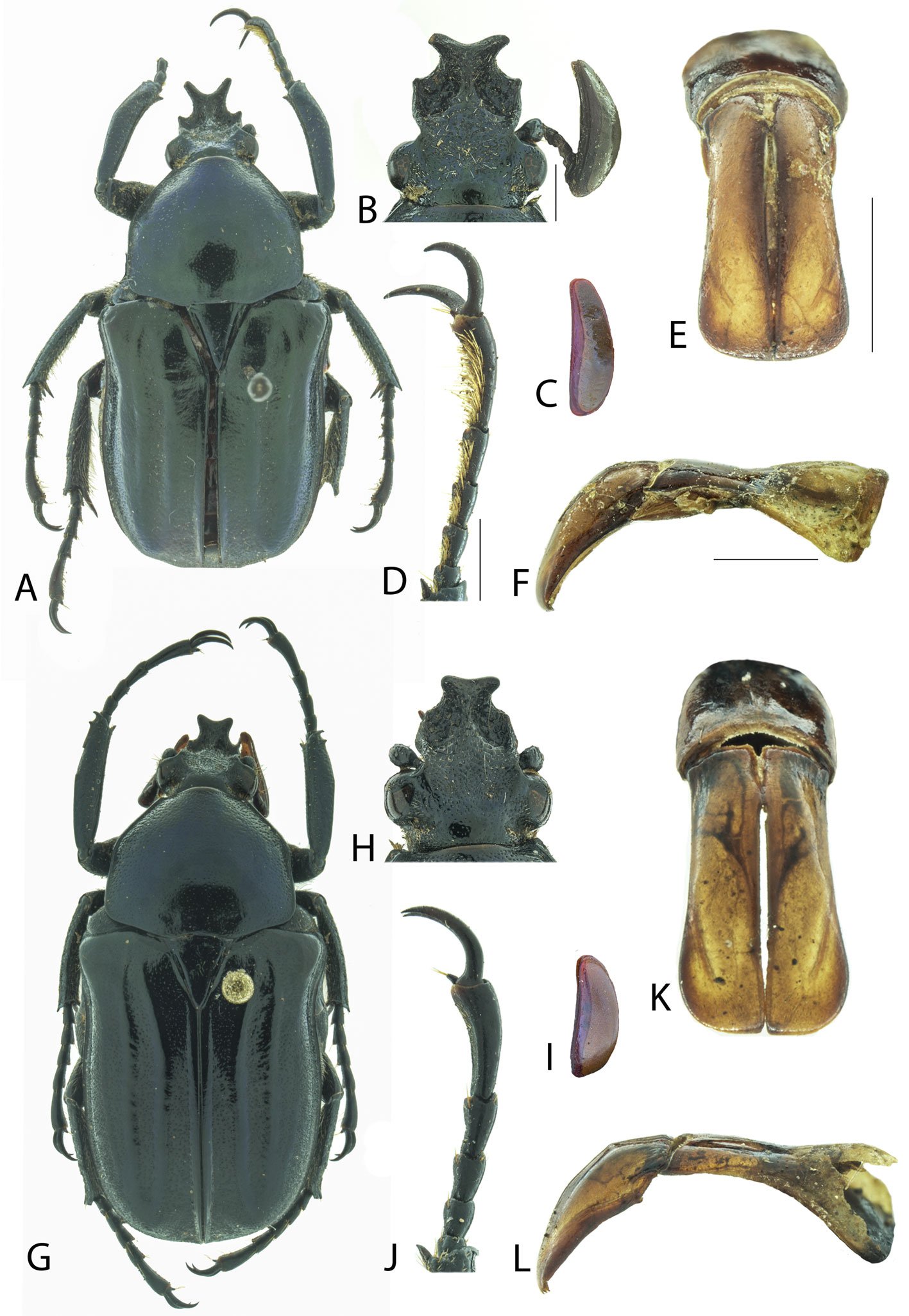
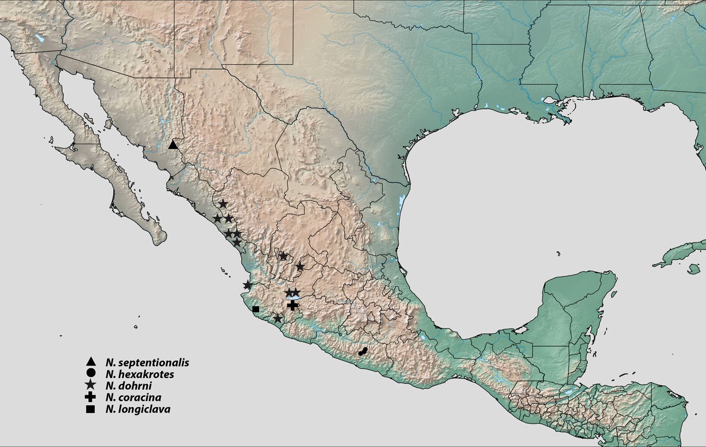
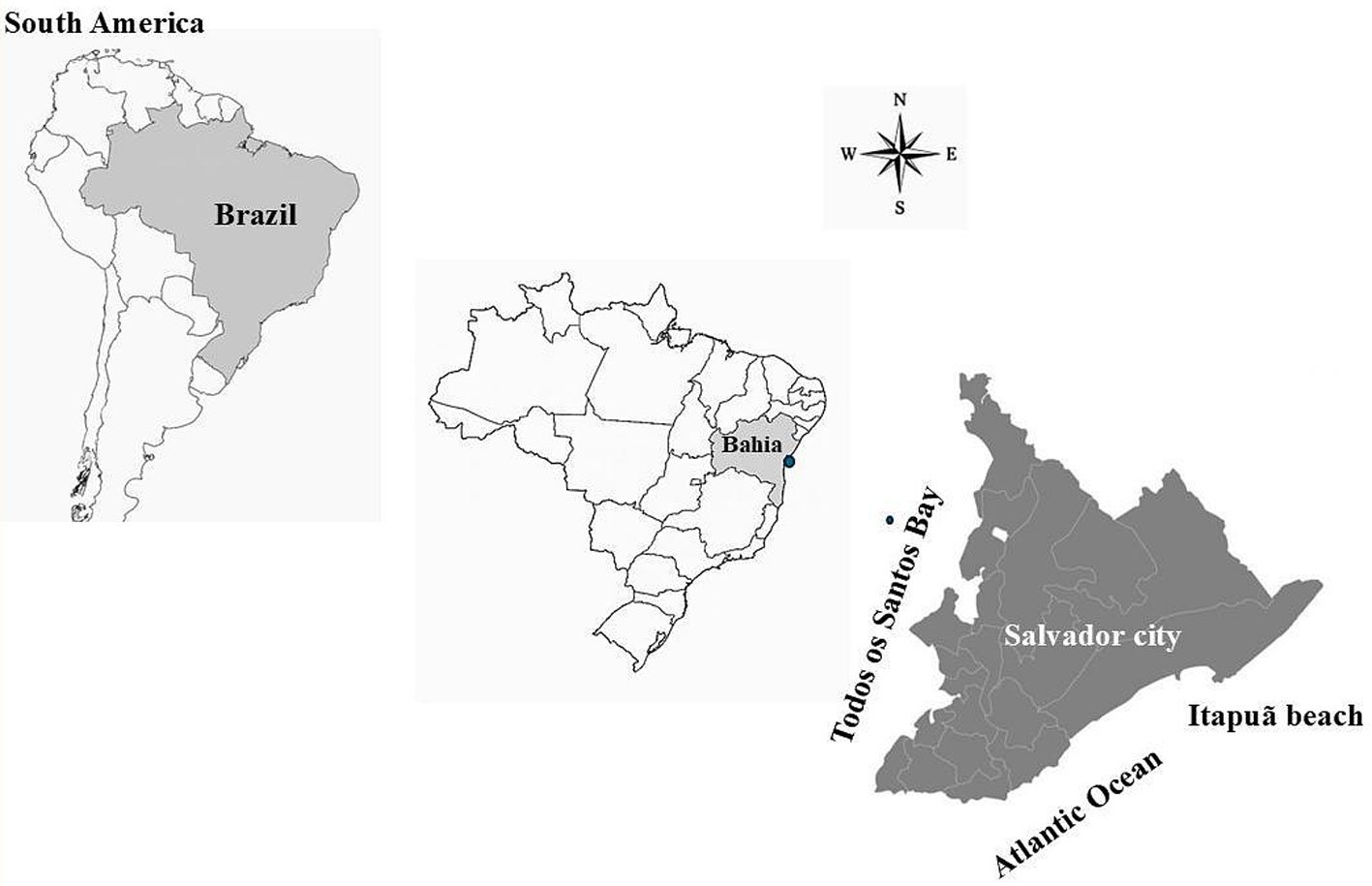


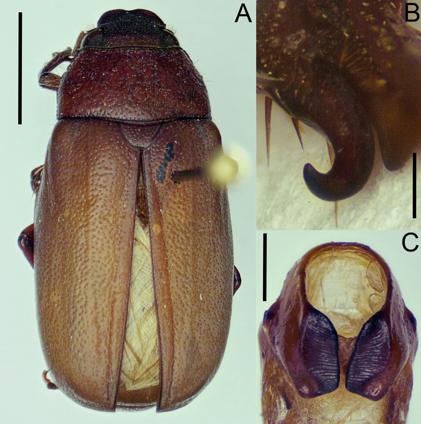


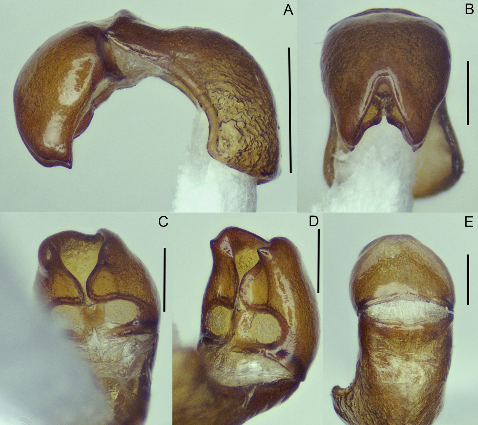


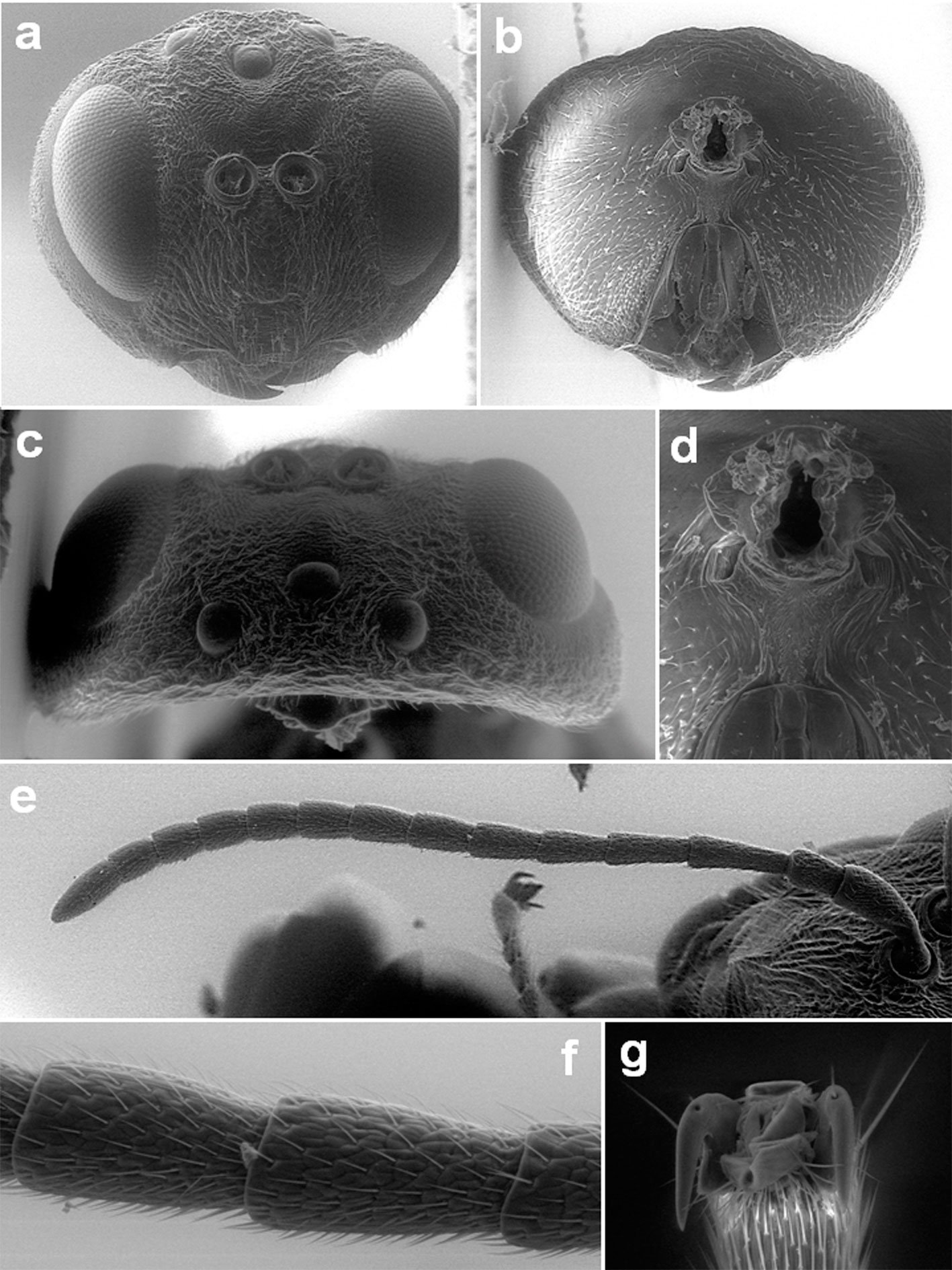

![Figure 3. Lateral habitus of a) Andricus protector sp. nova., b) A. formosalis [Picture obtained from Type Search of Smithsonian Entomological Collections, http://n2t.net/ark:/65665/m36fc57b94-797e-4d41-b88c-58776f4ed1d3]](https://rev-mex-biodivers.mx/wp-content/uploads/5448-Fig_3-12cm.jpg)