Vol. 88. núm. 1 (2017)
Marzo


Taxonomía y Sistemática
Ecología

Evolución

Biogeografía

Nuevos registros de babosas marinas (Gastropoda: Heterobranchia) para isla Clarión, archipiélago Revillagigedo, México
Héctor Alejandro Hernández-Castellanos a, *, Víctor Landa-Jaime a y Jesús Emilio Michel-Morfín b
a Universidad de Guadalajara, Centro Universitario de la Costa Sur, Departamento de Estudios para el Desarrollo Sustentable de Zonas Costeras, Gómez Farías Núm. 82, 48980 San Patricio-Melaque, Jalisco, México
b Universidad de Guadalajara, Centro Universitario de Ciencias Biológicas y Agropecuarias, Departamento de Ecología Aplicada, Camino Ramón Padilla Sánchez Núm. 2100, 45510 Zapopan, Jalisco, México
*Autor para correspondencia: hecalehercas96@gmail.com (H.A. Hernández-Castellanos)
Resumen
El archipiélago de Revillagigedo se ubica en el Pacífico este tropical y consta de 4 islas volcánicas, isla Clarión es la más occidental y remota de este parque marino de México. Esta región está influenciada por aguas frías provenientes de la corriente de California y aguas cálidas de la corriente Norecuatorial, lo que resulta en una zona de convergencia, con una alta biodiversidad marina. Clarión es una isla pequeña y distante, dominada por acantilados, con playas arenosas-rocosas en su cara sur, lo que se traduce en áreas poco accesibles para llevar a cabo investigaciones. El objetivo de esta contribución es dar a conocer una lista de especies de babosas marinas presentes en la isla. El estudio se llevó a cabo entre enero y marzo de 2023, y febrero-marzo de 2024, a través del muestreo continuo en playas, pozas intermareales y zonas arrecifales someras de la cara sur de la isla. En total, se registraron 14 especies de babosas marinas, 13 registros nuevos para esta isla y 5 para el archipiélago de Revillagigedo. Este estudio contribuye significativamente al conocimiento de la biodiversidad de las babosas marinas heterobranquias insulares del Pacífico tropical.
Palabras clave: Moluscos; Gasterópodos; Pacífico este tropical; Zona intermareal; Isla oceánica; Biodiversidad marina
New records of sea slugs (Gastropoda: Heterobranchia) from Clarion Island, Revillagigedo Archipelago, Mexico
Abstract
The Revillagigedo Archipelago is located on the East Tropical Pacific; it consists of 4 volcanic islands. Clarion Island is the most western and remote island of this marine national park. The region is influenced by the cold currents from California and the warm waters of the North Equatorial current, creating a convergence zone, with high marine biodiversity. Clarion is a small and distant island, dominated by high cliffs with rocky sandy beaches on the south side, with hard-to-access areas for research. The objective of this contribution is to provide a species list of the sea slugs present on the island. The study was performed from January to March 2023, and February to March 2024, through a continual survey of the beaches, intertidal pools and shallow reef areas in the south side of the island. In total, we recorded 14 species of sea slugs, 13 were new records for this island and 5 new records for the Revillagigedo Archipelago. This study significantly contributes to the knowledge of the biodiversity of island heterobranch sea slugs of the Tropical Pacific.
Keywords: Mollusks; Gastropods; Eastern Tropical Pacific; Intertidal zone; Oceanic island; Marine biodiversity
Introducción
El archipiélago de Revillagigedo es un conjunto de 4 islas de origen volcánico ubicadas en la ecorregión del Pacífico Transicional Mexicano. Se localiza en la zona de encuentro de las provincias Panámica, Californiana y de Cortés, en un área de convergencia de aguas frías provenientes de la corriente de California y aguas cálidas de la corriente Norecuatorial, lo que propicia valores altos de diversidad, tanto en tierra como en el océano (Conanp, 2018). Comprende, de mayor a menor tamaño, a las islas Socorro, Clarión, San Benedicto y el islote Roca Partida.
Clarión es la isla más occidental del Archipiélago (18°21’ N, 114°45’ O) (fig. 1A). Se ubica a 390 km al oeste de isla Socorro, 707 km al suroeste de Baja California Sur (Cabo San Lucas) y 1,100 km al oeste de Colima (Manzanillo) (Conanp, 2018). Comprende un área de 1,925 ha, 8.5 km de largo y 3.6 km de ancho y su punto más alto es el monte Gallegos (335 m snm; fig. 1A). En la zona oceánica predomina la influencia de las corrientes de California y la corriente Norecuatorial, con temperaturas del agua entre 20 y 28 °C. Presenta un régimen de mareas de tipo semidiurno, con oleaje alto y periodicidad de surgencias estacionales (Conanp, 2018). La costa de la isla está conformada por acantilados de entre 3 y 250 m de alto en sus lados norte, este y oeste, mientras que en la porción sur se localizan 3 playas arenosas, separadas entre ellas por formaciones rocosas. Estas playas se extienden por 2.5 km aproximadamente, lo que constituye 10% del litoral de la isla (Conanp, 2018; Holroyd y Trefy, 2010).
Las babosas marinas son moluscos de la subclase Heterobranchia, clase Gastropoda, que suelen presentar las branquias y el intestino en la parte posterior del cuerpo, proceso que ocurre en fases tempranas del desarrollo, además de carecer de concha externa en su mayoría (salvo algunas especies que poseen una pequeña concha, interna o externa) (Behrens et al., 2022; Hermosillo-González, 2006). Habitan en todos los océanos, desde la zona intermareal hasta las ventilas hidrotermales. La mayoría de especies son bentónicas, aunque algunas se adaptaron a vivir en la zona pelágica y unas pocas pueden ser encontradas en agua salobre (Camacho-García et al., 2005). Su tamaño va desde los 3 a los 1,000 mm en algunas especies, como es el caso de Aplysia vaccaria (Winkler, 1955) (Behrens et al., 2022; Camacho-García et al., 2005; Hermosillo et al., 2006). A excepción de los órdenes Aplysiida, algunos Cephalaspidea y el superorden Sacoglossa (cuyas dietas se basan en algas), todas las especies se consideran carnívoras (Behrens et al., 2022). Todas las babosas marinas heterobranquias son hermafroditas y se reproducen sexualmente (Behrens et al., 2022; Camacho-García et al., 2005; Hermosillo et al., 2006). Para el Pacífico este, se tienen descritas alrededor de 360 especies con algunas más en proceso de descripción (Behrens et al., 2022).
En el Pacífico este tropical (PET) se han llevado a cabo importantes estudios sobre la riqueza y distribución de este grupo de moluscos. La guía de campo de babosas marinas del PET de Camacho-García et al. (2005) describe 163 especies bentónicas. Behrens y Hermosillo (2005) y Gosliner (2010) reportaron 122 especies para las costas de California. Por su parte, la guía de babosas marinas del Pacífico de Hermosillo et al. (2006) contempla 234 especies para el litoral mexicano y es el trabajo más completo para esta región.
Las regiones insulares del PET han sido estudiadas por diferentes autores. Kaiser (1997) registra 54 especies para las islas Galápagos, Ecuador. Kaiser y Bryce (2001) registraron 27 especies en la isla de Malpelo, Colombia. Para el atolón francés de Clipperton, Kaiser (2007) registra la presencia de 35 especies. Finalmente, García-Méndez y Camacho-García (2016) incrementan en 13 el número de especies de babosas marinas en isla del Coco, Costa Rica, para compilar un total de 40 especies. En la península de Baja California destaca el trabajo de Sánchez-Ortíz (2000), quien registra 45 especies para las islas cercanas a Loreto y las localidades de La Paz, Cabo San Lucas, isla Cedros y bahía Tortugas; en el mismo año, Millen y Bertsch (2000) describen 3 especies nuevas para la misma región. Hermosillo y Valdés (2008) describieron 2 especies nuevas para el PET. Ortea y Llera (1981) describieron una especie endémica para isla Isabel. Para Bahía de Banderas, Hermosillo (2006) registró 140 especies y para la región compartida entre Colima, Michoacán y Guerrero, 76 especies fueron reportadas (Hermosillo y Behrens, 2005). Hermosillo-González (2006) reconoce que el Pacífico Transicional Mexicano comparte especies, tanto con la provincia Panámica, como con la provincia de California.
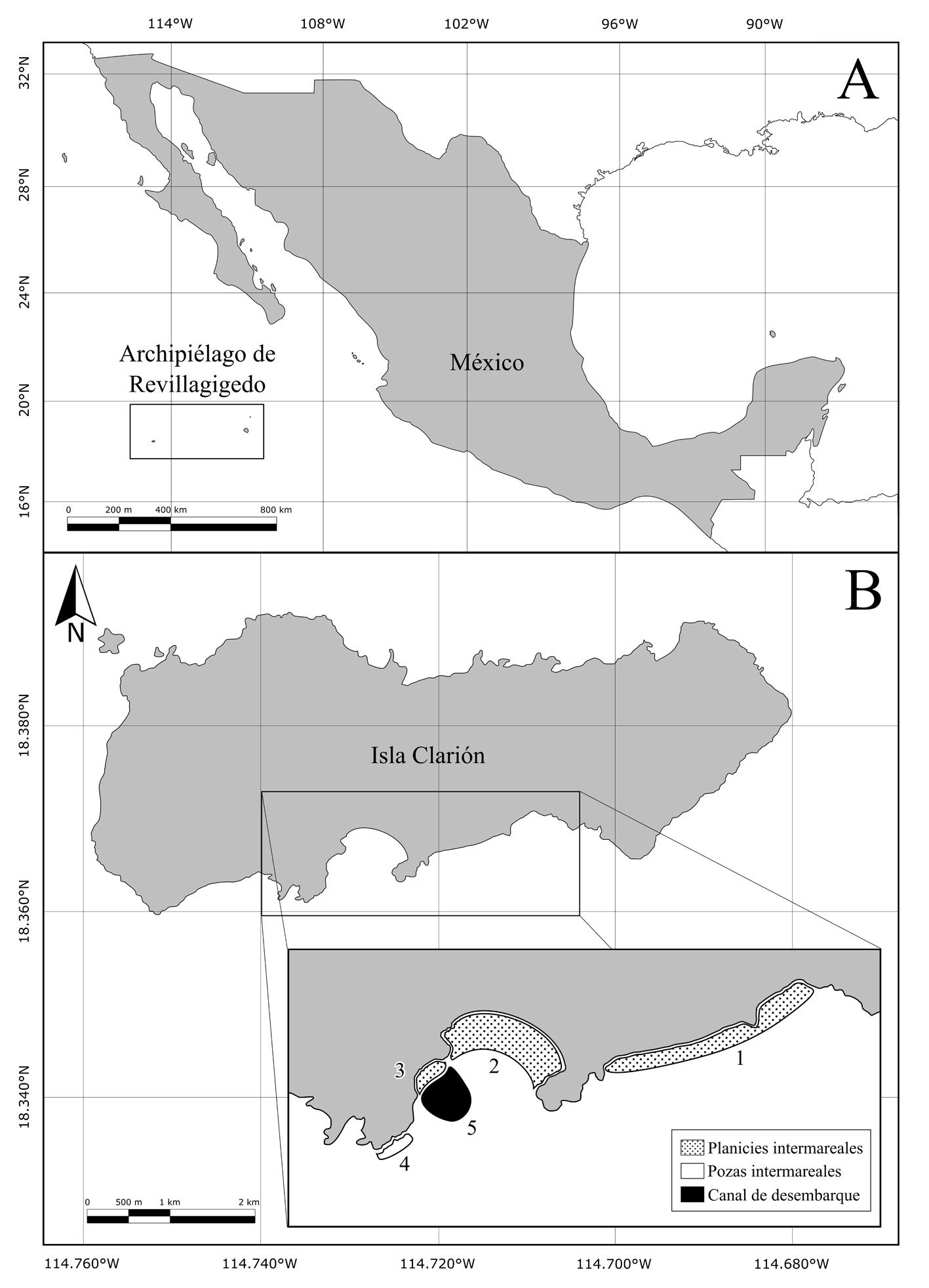
Figura 1. A, Ubicación de isla Clarión y el archipiélago de Revillagigedo en México; B, ubicación de los sitios de muestreo en isla Clarión: playa este (1), bahía Azufre (2), playa oeste (3), pozas intermareales (4) y canal de desembarque (5). Mapa por H. A. Hernández-Castellanos.
Por otra parte, los esfuerzos encaminados a incrementar el conocimiento de las babosas marinas en el archipiélago Revillagigedo han sido escasos. Hermosillo y Gosliner (2008) registraron 37 especies submareales para las 4 islas, sumando un total de 42 especies para este parque marino. En isla Socorro se obtuvo la mayor riqueza de especies, con 36 registros, mientras que fueron reportadas solamente 5 especies en isla Clarión. Behrens et al. (2009) describieron 1 especie nueva (Felimida socorroensis Behrens, Gosliner y Hermosillo, 2009) derivada del estudio de Hermosillo y Gosliner (2008).
El objetivo de este estudio fue incrementar el conocimiento sobre las babosas marinas del Pacífico de México al presentar nuevos registros para isla Clarión, derivados de observaciones realizadas en la zona intermareal y submareal somera, así como actualizar el número de estas especies de moluscos presentes en el archipiélago de Revillagigedo.
Materiales y métodos
Se realizaron observaciones en diferentes zonas de la porción sur de isla Clarión: en la zona intermareal de las playas, la zona de pozas intermareales y el canal de desembarque (fig. 1B). La porción sur es la única área del litoral de la isla por la cual se puede acceder de manera segura a la zona intermareal. Dentro de esta porción, se definieron 5 sitios principales de muestreo: 1) playa este, con una superficie de 17 ha, se compone de fragmentos de coral y arena, es una planicie de aproximadamente 150 m de ancho en su parte más amplia, que queda expuesta durante la bajamar y en la cual hay algunas rocas y cabezas grandes de coral, así como pozas y canales intermareales; 2) bahía Azufre, se encuentra en el centro de la cara sur de la isla y se drena casi por completo durante la bajamar, exponiendo 19 ha de litoral conformado por sustrato arenoso en el centro, rocas en los extremos este y oeste, y canales y pozas intermareales en el centro-sur (fig. 2). En la entrada de la bahía se encuentra el área con mayor cobertura de arrecife de coral del archipiélago (Ketchum y Reyes-Bonilla, 2009), el cual queda parcialmente expuesto durante la bajamar; 3) playa oeste: se encuentra en el extremo oeste de la bahía Azufre. Es la más pequeña de las 3 playas (0.7 ha) y consiste en una caleta independiente, adyacente al canal de desembarque. Se conforma principalmente de sustrato rocoso con algunos parches arenosos y rocas grandes sueltas. Al igual que las otras playas, durante la bajamar queda expuesta un área considerable, donde hay canales y pozas intermareales; 4) pozas intermareales, consisten en una serie de 3 pozas relativamente grandes (~ 50-170 m2 cada una) con comunicación intermitente con el océano. Se ubican debajo del “cerro del faro” y todas poseen profundidades entre 1 y 4 m, conteniendo sustrato rocoso y algunos parches arenosos; 5) canal de desembarque: consiste en una zanja tallada en el fondo rocoso-coralino, acondicionada por personal de la Marina mexicana para facilitar el desembarque en la isla. Tiene una longitud aproximada de 30 m y un ancho que va aumentando de 2 a 10 m conforme se aleja de la línea de costa. El sustrato es arenoso y rocoso, y se encuentra rodeado por arrecife coralino. La profundidad va de 20 cm a 10 m en la parte más alejada de tierra firme.
Los sitios de muestreo en intermareal somero fueron seleccionados por su accesibilidad durante los eventos de marea baja, al ser estos los momentos en los que se puede realizar una búsqueda activa de los especímenes en la zona. Por la misma razón, las búsquedas en el intermareal profundo se realizaron durante la pleamar, siendo éste el momento más accesible a estas zonas. Se llevaron a cabo 40 muestreos en la zona intermareal de las 3 playas arenosas-rocosas, el canal de desembarque y la zona de pozas intermareales adyacente al faro de la isla durante enero, febrero y marzo de 2023, y febrero y marzo de 2024. Para las playas este y oeste, bahía Azufre y la parte somera del canal de desembarque, se trazaron transectos de entre 80 y 350 m de longitud × 3 m de ancho (dependiendo de la morfología y extensión del sitio de muestreo), 2 h antes y 2 h después de la bajamar de las mareas vivas (3 días antes y 3 días después de las lunas nueva y llena), revisando exhaustivamente tanto en la superficie del sustrato como debajo de rocas y cabezas de coral sueltas, cada 2 a 5 m, aproximadamente. Para la zona de pozas intermareales y el canal de desembarque se realizó el mismo proceso 2 veces por semana, pero haciendo uso de equipo de buceo libre, entre 40 cm y 2 m de profundidad. Se seleccionaron horarios diurnos y vespertinos variables durante los eventos de marea alta, 2 h antes y 2 h después de la pleamar. Una vez localizado un organismo, se fotografió a detalle, mostrando tanto las características del ejemplar como de la fauna y flora acompañantes, así como el sustrato donde se encontró. Para ello, se utilizó una cámara Olympus Tough TG6 con el modo “Macro-Microscope”, con un aumento entre 2.9x y 11x. La profundidad donde se encontró cada organismo fue registrada con el profundímetro integrado en la cámara, el cual cuenta con una precisión de 10 cm. Se tomaron numerosas fotografías de cada ejemplar, las cuales fueron almacenadas y posteriormente revisadas a detalle. Todas las fotografías fueron tomadas por el primer autor de este estudio.
De acuerdo con los lineamientos consignados en el Programa de Manejo del Parque Nacional Archipiélago de Revillagigedo (Conanp, 2018), ningún ejemplar fue recolectado, manipulado o extraído de su hábitat para este estudio, por lo que la identificación de los ejemplares se realizó mediante las fotografías obtenidas, la observación posterior y la comparación de caracteres morfológicos (como la coloración principal del manto, rinóforos y branquias, así como la presencia o ausencia de estructuras [ceratas, apéndices] y marcas o patrones de coloración) con las guías de identificación disponibles para esta zona geográfica, así como listados históricos (Behrens et al., 2022; Camacho-García et al., 2005; Hermosillo y Gosliner, 2008; Hermosillo et al., 2006). La validez taxonómica que se presenta para cada una de las especies y géneros fue revisada de acuerdo con el World Register of Marine Species (WoRMS Editorial Board, 2024), así como con la autoridad taxonómica. El arreglo taxonómico desde orden y superorden hasta la especie fue el utilizado por Behrens et al. (2022) y por Bouchet et al. (2017).
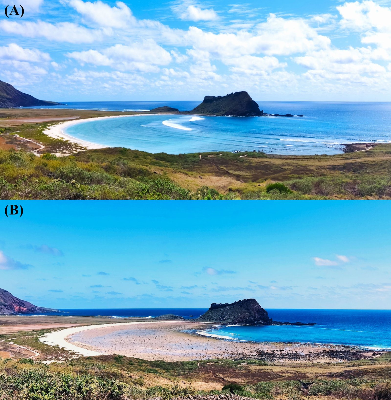
Figura 2. Comparación de la bahía Azufre durante la altamar (A) y la bajamar (B).
Resultados
Se registraron 143 ejemplares de moluscos gasterópodos de la subclase Heterobranchia pertenecientes a 14 especies, en los 5 sitios del intermareal de isla Clarión.
Phylum Mollusca Linnaeus, 1758
Clase Gastropoda Cuvier, G. 1795
Subclase Heterobranchia (Burmeister y Hermann, 1837)
Orden Cephalaspidea P. Fischer, 1883
Familia Aglajidae Pilsbry, 1895
Navanax aenigmaticus (Bergh, 1893). Fig. 3A.
Material examinado: 17 ejemplares.
Descripción. Concha interna. El cuerpo es café con manchas color crema y puede variar a rosa fuerte o café claro. Tiene una serie de puntos azul turquesa a lo largo del margen interior de los parapodios. La parte ventral del cuerpo es negra con puntos amarillos y blancos y alcanza los 75 mm de longitud (Behrens et al., 2022).
Ecología y hábitat. Todos los organismos fueron observados debajo de rocas, sobre sustrato arenoso y rocoso en las 3 playas y el canal de desembarque, a profundidades de entre 10 cm y 2 m de profundidad.
Distribución. Desde San Diego, California, Bahía Vizcaíno, Baja California, México, a Panamá; islas Galápagos, Ecuador, este y oeste del Atlántico tropical (Behrens et al., 2022).
Observaciones. Nuevo registro para isla Clarión. Visto en pareja en una ocasión. Seis variedades fueron identificadas gracias a las diferencias en la pigmentación (coloración y patrones), se clasificaron como marrón, café claro, café oscuro, negro, oliva y ocre (material suplementario: fig. S1). Carece de rádula. Se alimenta de otras babosas marinas heterobranquias, como notaspídeos y nudibranquios (Behrens et al., 2022).
Familia Haminoeidae Pilsbry, 1895
Haminoea virescens (G. B. Sowerby II, 1833). Fig. 3B.
Material examinado: 1 ejemplar.
Descripción. Concha expuesta, verde, con la espira hundida (material suplementario: fig. S2). Diferente de H. vesicula en la abertura mayor. Cuerpo verde con puntos amarillos en el escudo cefálico y manchas amarillo y blanco en los parapodios. Llega a medir 45 mm de longitud (Behrens et al., 2022).
Ecología y hábitat. Observado después del atardecer y sobre sustrato arenoso en la Bahía Azufre, aproximadamente a 15 cm de profundidad.
Distribución. Desde Alaska, EUA, hasta Panamá (Behrens et al., 2022).
Observaciones. Nuevo registro para isla Clarión y el Archipiélago. Habita en áreas rocosas intermareales en marea baja.
Superorden Sacoglossa Ihering, 1876
Familia Caliphyllidae Tiberi, 1881
Cyerce orteai Valdés y Camacho-García, 2000. Fig. 3C.
Material examinado: 68 ejemplares.
Descripción. El color varía desde crema pálido con algunas incrustaciones blancas, hasta verde oliva con puntos verde claro y café. La cabeza tiene puntos blancos opacos y un par de áreas color crema claro alrededor de los ojos. Los rinóforos y tentáculos orales apuntan hacia adelante. Las ceratas son grandes, redondas e infladas, cubiertas de tubérculos. Alcanza los 20 mm de longitud (Behrens et al., 2022).
Ecología y hábitat. Se observó en las 3 playas y el canal de desembarque, entre 5 y 50 cm de profundidad, sobre sustrato arenoso, rocoso y entre la vegetación y fragmentos de coral. Ocasionalmente en parejas y/o acompañada de masas ovígeras (material suplementario: fig. S3).
Distribución. Desde La Paz, Baja California, hasta Costa Rica, Hawaii y Okinawa (Behrens et al., 2022).
Observaciones. Nuevo registro para isla Clarión y el archipiélago. Hermosillo et al. (2006) mencionan que esta especie es de hábitos nocturnos y se alimenta del alga Halimeda. Fue la especie más abundante en este estudio. C. orteai ha sido registrada previamente en Baja California Sur, Costa Rica y en la isla de Oahu (Hawaii) (Behrens et al., 2022; Hermosillo et al., 2006; Valdés y Camacho-García, 2000). Sin embargo, no había sido observada en el archipiélago Revillagigedo, a pesar de encontrarse en el mismo corredor biogeográfico.
Polybranchia mexicana Medrano, Krug, Gosliner, Biju Kumar y Valdés, 2018. Fig. 3D.
Material examinado: 1 ejemplar.
Descripción. Cuerpo translúcido variable del amarillo al verde claro, con pequeños lunares blancos. Los rinóforos bifurcados están orientados al frente. Las ceratas tienen pequeñas manchas negras y las glándulas digestivas son visibles. Los rinóforos no poseen papilas. Llega a medir 12 mm (Behrens et al., 2022).
Ecología y hábitat. Observada a 1.5 m de profundidad en la zona de pozas intermareales.
Distribución. Desde el sur de Baja California Sur, México, hasta las islas Galápagos (Medrano et al., 2018).
Observaciones. Nuevo registro para isla Clarión y el archipiélago. Especie descrita recientemente por Medranoet al.(2018). Anteriormente pertenecía al complejo de especies dentro de P. viridis. Se trata de una especie nocturna con la capacidad de autotomizar sus ceratas cuando es molestada.
Orden Aplysiida [= Anaspidea] P. Fischer, 1883
Familia Aplysiidae Lamarck, 1809
Dolabella cf. auricularia (Lighfoot, 1786). Fig. 3E.
Material examinado: 1 ejemplar.
Descripción. La parte posterior del cuerpo forma un disco en diagonal, con papilas en toda la orilla y un sifón exhalante en el centro (material suplementario: fig. S4). Es de color muy variable, pero usualmente presenta tonos moteados de verde o café, lo que le da un muy buen camuflaje. Produce tinta cuando es molestada. Alcanza 500 mm de longitud (Behrens et al., 2022).
Ecología y hábitat. Solo fue observada en una ocasión, a 1.5 m de profundidad en una de las pozas intermareales, parcialmente enterrada en sustrato arenoso.
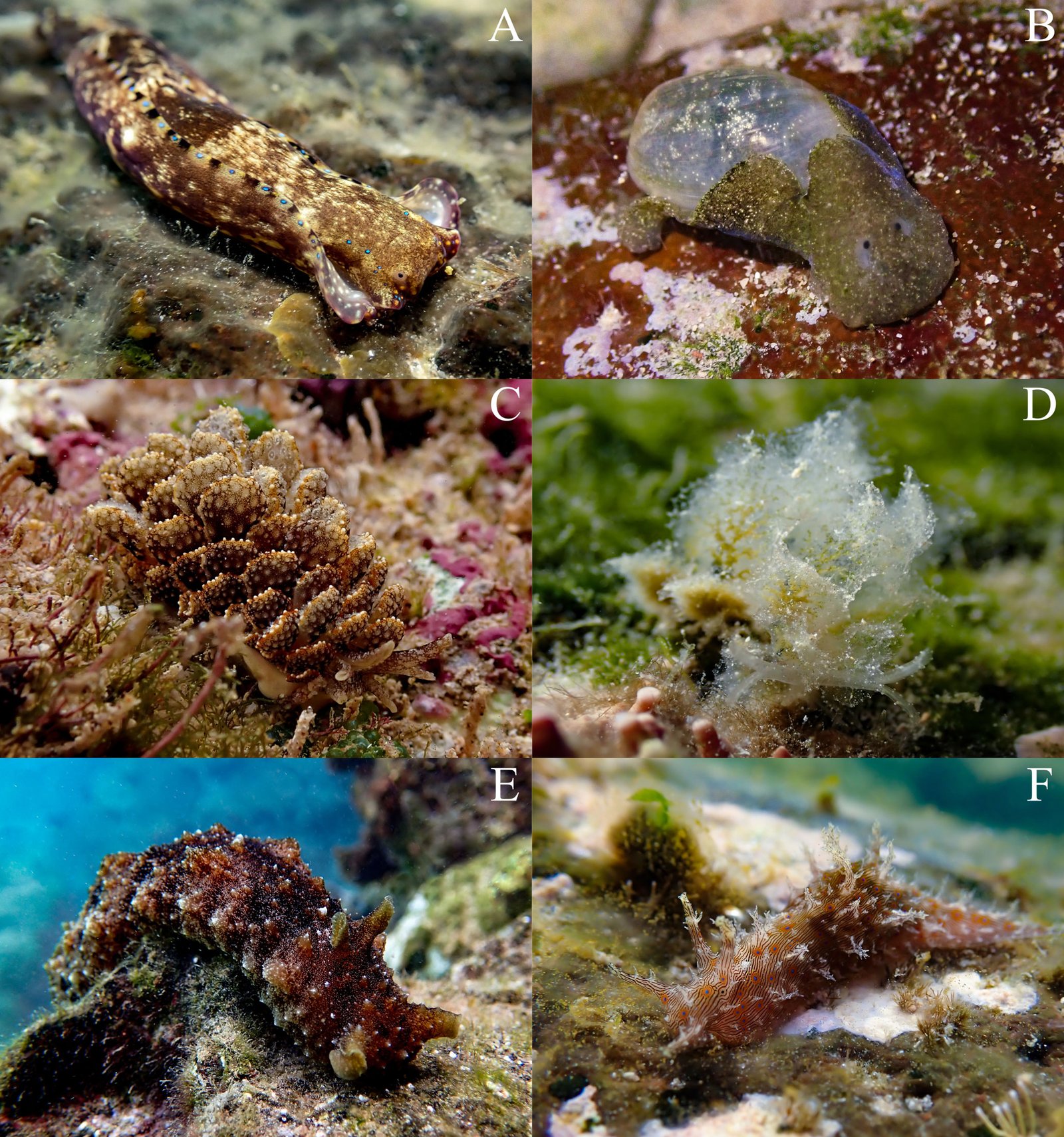
Figura 3. Babosas marinas heterobranquias de isla Clarión, archipiélago de Revillagigedo, observadas en este estudio (Cephalaspidea, Sacoglossa y Aplysiida). La talla aproximada se encuentra entre paréntesis.A, Navanax aenigmaticus (35 mm); B, Haminoea virescens (15 mm); C, Cyerce orteai (40 mm); D, Polybranchia mexicana (10 mm); E, Dolabella cf. auricularia (90 mm); F, Stylocheilus ricketsii (35 mm).
Distribución. Especie circumtropical (Behrens et al., 2022).
Observaciones. Nuevo registro para isla Clarión. Es citada como especie nocturna. Rara vez observada durante el día, aunque en este estudio se observó alrededor de las 10:00 h. Behrens et al. (2022) consideran que existe evidencia de que D. cf. auricularia es en realidad un complejo de varias especies no descritas en su totalidad; a la fecha de realización de esta contribución, el nombre Dolabella. cf. auricularia es válido para esta especie.
Stylocheilus ricketsii (MacFarland, 1966). Fig. 3F.
Material examinado: 3 ejemplares.
Descripción. Cuerpo alargado y pequeño en comparación con otras especies de la misma familia. Líneas oscuras irregulares longitudinales, con puntos azules dispersos. Posee apéndices ramificados por todo el cuerpo, así como una pequeña joroba y cola alargada. Alcanza 65 mm y libera tinta cuando es molestada (material suplementario: fig. S5) (Behrens et al., 2022).
Ecología y hábitat. Observado debajo de rocas en sustrato arenoso con presencia de algas del género Halimeda.
Distribución. Desde Baja California, México, hasta las islas Galápagos (Behrens et al., 2022).
Observaciones. Nuevo registro para isla Clarión. Especie críptica, difícil de ver entre las algas del fondo.
Orden Pleurobranchida [Pleurobranchoidea] Gray, 1827
Familia Pleurobranchidae Gray, 1827
Berthella martensi (Pilsbry, 1896). Fig. 4A.
Material examinado: 1 ejemplar.
Descripción. Variable en su coloración, desde blanco a anaranjado y marrón intenso. Branquia bajo el manto en el lado derecho del cuerpo. Esta especie tiene lunares característicos más oscuros que el cuerpo y frecuentemente una banda oscura en la orilla del manto y pie. Alcanza 70 mm de longitud total (Behrens et al., 2022).
Ecología y hábitat. Solo fue observada una vez, a 1.5 m de profundidad en el canal de desembarque, bajo una roca grande en sustrato rocoso.
Distribución. Desde Las Arenas, Baja California, hasta Panamá; también citada para el Indopacífico (Behrens et al., 2022).
Observaciones. Nuevo registro para isla Clarión. Al igual que otras especies de babosas, esta especie tiene la capacidad de autotomizar partes de su manto cuando es molestada.
Berthella grovesi Hermosillo y Valdés, 2008. Fig. 4B.
Material examinado: 1 ejemplar.
Descripción. El cuerpo es ovalado. El manto sobresale el ancho del pie, cubriendo completamente las branquias, el velo bucal y los rinóforos parcialmente. Estos últimos son enrollados, cortos, robustos y unidos basalmente. El pie es bilabiado. El color del fondo varía de un marrón rosado claro a uno más oscuro. Esta especie llega a medir 30 mm de longitud (Behrens et al., 2022).
Ecología y hábitat. Solo fue observada una vez bajo una roca pequeña sobre sustrato rocoso en la playa oeste, a 10 cm de profundidad.
Distribución. Registrada en isla Isabel y Bahía de Banderas, México y Panamá (Behrens et al., 2022).
Observaciones. Nuevo registro para isla Clarión y el archipiélago. Se encuentra bajo rocas en la zona intermareal y submareal somero. Esta es la observación más alejada del litoral continental publicada hasta ahora (707 km al suroeste de Baja California Sur y 1,100 km al oeste de Colima), reportada previamente en isla Isabel, Nayarit; en el Parque Nacional Coiba en Panamá y en el litoral continental mexicano (Bahía de Banderas en Jalisco-Nayarit, Manzanillo en Colima y Caleta de Campos en Michoacán) (Behrens et al., 2022; Hermosillo et al., 2006; Hermosillo y Valdés, 2008).
Berthella cf. agassizii (MacFarland, 1909). Fig. 4C.
Material examinado: 2 ejemplares.
Descripción. El cuerpo es translúcido y va del rosa a café claro, en ocasiones con puntos blancos dispersos. Los rinóforos están enrollados y la superficie dorsal se aprecia arrugada. Alcanza 12 mm (Behrens et al., 2022).
Ecología y hábitat. Solo observada en una ocasión, a 80 cm de profundidad en el canal de desembarque, debajo de una roca grande en sustrato rocoso.
Distribución. En el océano Pacífico, desde Punta Eugenia, Baja California, hasta Panamá. En el océano Atlántico, desde el mar Caribe hasta Santa Catarina, Brasil (Behrens et al., 2022).
Observaciones. Nuevo registro para isla Clarión. De acuerdo con Behrens et al. (2022), B. agassizii fue descrita originalmente para Brasil. Dado el distanciamiento geográfico, diferencias en tamaño, color y tracto reproductivo entre ambas especies (Pacífico y Atlántico), se consideran especies distintas (Alvim y Pimienta, 2015). Sin embargo, a la fecha de escritura de este documento, Berthella cf. agassizii es un nombre válido para la especie observada.
Orden Nudibranchia Cuvier, 1817
Familia Dendrodorididae O’Donoghue, 1924
Dendrodoris cf. fumata (Rüpell y Leuckart, 1831). Fig. 5A, B.
Material examinado: 21 ejemplares.
Descripción. Típico nudibranquio dórido, tiene el manto altamente ondulado. Se reconocen 3 variaciones de color: cuerpo negro aterciopelado con una línea roja en el margen, cuerpo blanquecino translúcido y cuerpo anaranjado o rojo. Todas las variaciones presentan puntas blancas en los rinóforos y en la pluma branquial, que es de gran tamaño. Alcanza una longitud total corporal de 30 mm (Behrens et al., 2022).
Ecología y hábitat. Se observó en las 3 playas en sustrato rocoso, arenoso y en zonas con coral, entre 10 y 50 cm de profundidad. Se identificaron las 3 coloraciones descritas para esta especie, además de la coloración propia de los juveniles: rojo (juvenil), negro, rojinegro y blanco, siendo este último el más abundante (material suplementario: fig. S6). En ocasiones fue visto en pareja.
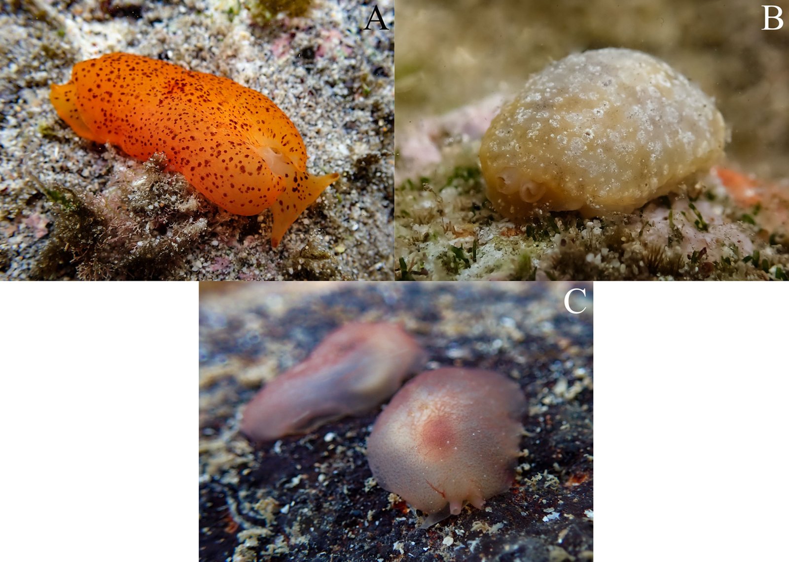
Figura 4. Babosas marinas heterobranquias de isla Clarión, archipiélago de Revillagigedo, observadas en este estudio (Pleurobranchida). La talla aproximada se encuentra entre paréntesis.A, Berthella martensi (35 mm); B, Berthella grovesi (30 mm); C, Berthella cf. agassizii (15-20 mm).
Distribución. Desde bahía Vizcaíno, Baja California, hasta Costa Rica, Panamá y las islas Galápagos, Ecuador (Behrens et al., 2022).
Observaciones. Fue el nudibranquio más abundante, así como la única especie de este estudio reportada previamente para isla Clarión (Hermosillo y Gosliner, 2008). Nombrada así por el color de la variación oscura. Según Behrens et al. (2022), D. fumata es una especie ampliamente distribuida en el Indopacífico, genéticamente distinta a la presente en el Pacífico este tropical. Sin embargo, Dendrodoris cf. fumata es un nombre válido para esta especie a la fecha de escritura de este documento (Behrens et al., 2022; Valdés, Á., com. pers., 13 de julio de 2023).
Dendrodoris nigromaculata (Cockerell, 1905). Fig. 5C.
Material examinado: 2 ejemplares.
Descripción. Tiene el cuerpo alargado con márgenes ondulados. Su color va de blanco a crema con una serie de manchas de color chocolate o marrón de diferentes tamaños y cantidades. Las manchas se observan en 3 grupos, uno justo detrás de los rinóforos, otro en la parte central del cuerpo y una más anterior a la branquia, la cual es de color blanco o crema (al igual que los rinóforos). Alcanza una longitud corporal de 27 mm (Behrens et al., 2022).
Ecología y hábitat. Se registró en la playa oeste en sustrato rocoso, entre 10 y 20 cm de profundidad.
Distribución. Carmel, California; isla Guadalupe y las islas San Benito, Baja California (Behrens et al., 2022).
Observaciones. Nuevo registro para isla Clarión y el archipiélago. Los ejemplares fueron registrados en el intermareal y submareal somero. Este es el registro más meridional para esta especie, ya que anteriormente había sido registrada hasta las islas San Benito, Baja California (Behrens et al., 2022; Camacho-García et al., 2005; Goddard y Valdés, 2015; Hermosillo et al., 2006; Millen y Bertsch, 2005). Esta observación amplía su distribución y agrega a esta especie a la provincia del Pacífico Transicional Mexicano.
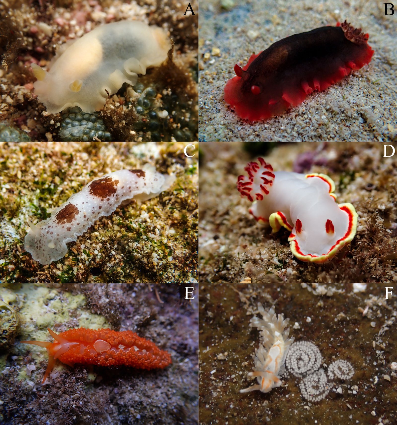
Figura 5. Babosas marinas heterobranquias de isla Clarión, archipiélago de Revillagigedo, observadas en este estudio (Nudibranchia). La talla aproximada se encuentra entre paréntesis.A, Dendrodoris cf. fumata var.blanca(25 mm); B, D. cf. fumata var. negra (30 mm); C, Dendrodoris nigromaculata (30 mm); D, Chromolaichma sedna (40 mm); E, Anteaeolidiella ireneae (30 mm); F, Anteaeolidiella lurana (10 mm).
Familia Chromodorididae Bergh, 1891
Chromolaichma sedna (Ev. Marcus & Er. Marcus, 1967). Fig. 5D.
Material examinado: 17 ejemplares.
Descripción. El cuerpo es de color blanco, con una banda amarilla delgada y otra de color rojo brillante, un poco más ancha rodeando el manto, el pie y la cola. Los rinóforos y branquias son blancos con puntas rojas (material suplementario: fig. S7B). Alcanza 65 mm de longitud (Behrens et al., 2022).
Ecología y hábitat. Observada en las playas este y oeste, entre 5 y 15 cm de profundidad, siempre bajo rocas en sustrato rocoso y arenoso.
Distribución. Desde el golfo de California y el Pacífico mexicano, hasta Panamá, Colombia, Ecuador y el Caribe (Behrens et al., 2022).
Observaciones. Nuevo registro para isla Clarión. Especie gregaria que se alimenta de esponjas. Observada en cópula en una ocasión (fig. S7A). Su coloración brillante es probablemente aposemática (Behrens et al., 2022).
Familia Aeolidiidae Gray, 1827
Anteaeolidiella ireneae Carmona, Bhave, Salunkhe, Pola, Gosliner y Cervera, 2014. Fig. 5E.
Material examinado: 7 ejemplares.
Descripción. El cuerpo es de color blanco translúcido, con pigmentación naranja dispersa sobre la espalda. Hay una línea blanca irregular desde la cabeza, que inicia entre los rinóforos y se extiende en forma de lágrima sobre el pericardio. Esta línea continua como varias manchas en forma de diamante de pigmento blanco o amarillo pálido a lo largo de la línea media. Los rinóforos y los tentáculos orales son de color naranja con puntas blancas. Las ceratas son largas y cilíndricas con puntas redondeadas, y se extienden desde la parte trasera de los rinóforos hasta la cola, dejando una zona desnuda sobre el dorso; son de color naranja brillante o gris oscuro, con una banda blanca y una punta blanca, y están dispuestas en hasta 36 filas, con hasta 12 ceratas en las filas anteriores y tan solo 4 en las últimas filas. Alcanza una longitud total de 12 mm (Behrens et al., 2022; Carmona et al., 2014).
Ecología y hábitat. Registrada en las playas este y oeste, bajo fragmentos de coral grandes y sobre sustrato rocoso, entre 5 y 20 cm de profundidad.
Distribución. En el Pacífico oriental. Ha sido registrada en México, Costa Rica y Panamá (Carmona et al., 2014).
Observaciones. Nuevo registro para isla Clarión. Esta especie fue descrita a partir de especímenes recolectados bajo coral suelto y arena en isla Clipperton. Recientemente, A. indica atravesó por una reestructuración taxonómica, pasando de ser una especie con una distribución circumtropical, a 8 nuevas especies. A. ireneae se distribuye en Clipperton, Revillagigedo, Panamá y Costa Rica (Behrens et al., 2022; Carmona et al., 2014).
Anteaeolidiella lurana (Ev. Marcus et Er. Marcus, 1967). Fig. 5F.
Material examinado: 2 ejemplares.
Descripción. Cuerpo delgado y alargado, con una cola relativamente corta. El cuerpo es de color blanco traslúcido, con una mancha en forma de herradura en la cabeza y que se extiende desde la base de los rinóforos hasta la base de los tentáculos orales. Posee 2 líneas onduladas anaranjadas discretas, que se extienden desde la parte posterior de la cabeza hasta encontrarse en la cola, formando diamantes blancos entre ellas. Los rinóforos y los tentáculos orales poseen pigmentación naranja en su base. Las ceratas son largas y más gruesas en la parte superior. Se extienden desde la parte posterior de los rinóforos hasta la cola. El epitelio de las ceratas está cubierto con pigmento naranja difuminado. Alcanza 12 mm de longitud (Carmona et al., 2014).
Ecología y hábitat. Observada en el canal de desembarque a 10 cm de profundidad.
Distribución. Posee una amplia distribución circumtropical: península de Yucatán y mar Caribe hasta Brasil; mar Mediterráneo y las islas Canarias; Australia (Carmona et al., 2014). En el Pacífico oriental ha sido registrada en el archipiélago de Revillagigedo (isla Socorro) y Bahía de Banderas, Nayarit, México (Carmona et al., 2014).
Observaciones. Nuevo registro para isla Clarión. Observada junto a masas ovígeras. Al igual que A. ireneae, esta especie fue recientemente separada de A. indica (Carmona et al., 2014).
Discusión
Todas las especies reportadas en este estudio constituyen nuevos registros para isla Clarión, a excepción de D. cf. fumata, que había sido previamente citada por Hermosillo y Gosliner (2008). Además, de las 14 especies observadas en este estudio, 5 representan registros nuevos para todo el archipiélago Revillagigedo (H. virescens, P. mexicana, C. orteai, B. grovesi y D. nigromaculata) (tabla 1). Este estudio incrementa de manera notable el conocimiento de las especies de babosas marinas de la zona intermareal en isla Clarión y el archipiélago de Revillagigedo. Constituye el primero de su tipo para isla Clarión y complementa el trabajo desarrollado por Hermosillo y Gosliner (2008), el cual se enfocó principalmente en especies de la zona submareal.
Con los registros nuevos presentados en esta investigación, se incrementa el número de babosas marinas de 42 a 47 especies para el Parque Nacional Archipiélago de Revillagigedo, y de 5 a 18 especies para isla Clarión. Esta riqueza de especies de babosas marinas en el archipiélago es equiparable a la riqueza registrada en otras islas y archipiélagos del PET, como isla Clipperton, Francia (Kaiser, 2007), isla del Coco, Costa Rica (García-Méndez y Camacho-García, 2015), isla de Malpelo, Colombia (Kaiser y Bryce, 2001) y las islas Galápagos, Ecuador (Kaiser, 1997) (tabla 2). No obstante, será necesario llevar a cabo estudios similares en las otras islas del archipiélago y a profundidades mayores a las de la zona submareal para conocer de mejor manera la biodiversidad de este grupo taxonómico en la región. De la misma manera, es importante complementar esta contribución con estudios moleculares para confirmar algunas de las incertidumbres taxonómicas actuales y poder realizar estudios de filogeografía y conectividad en el Pacífico este tropical. Además, es necesario incrementar el esfuerzo de estudio en las otras islas y zonas continentales del Pacífico de México.
Dedicar esfuerzos para incrementar el conocimiento de grupos de invertebrados poco estudiados en el archipiélago permitirá contar con una línea base más completa de la biodiversidad de este parque nacional y brindará elementos para determinar la efectividad de las medidas de manejo que buscan la protección de esta importante zona marina, considerada patrimonio de la humanidad (UNESCO, 2016). Finalmente, la ubicación del archipiélago, así como el hecho de ser la isla más alejada del territorio mexicano convierte a isla Clarión en un importante punto de investigación y un laboratorio natural para observar y comprender diferentes procesos ecológicos.
Agradecimientos
A la Secretaría de Marina y al Grupo de Ecología y Conservación de Islas por el apoyo logístico durante el viaje y la estancia en isla Clarión. A Ángel Valdés y a Alicia Hermosillo por su valioso apoyo en la identificación de algunos ejemplares y facilitar material bibliográfico. A los estudiantes de la licenciatura en Biología Marina de la Universidad de Guadalajara, Joshua Martín y Lizely Estrada por su colaboración en el trabajo de campo, y finalmente a la bióloga Elizabeth Piña Vera por su compañía y apoyo durante todo el proceso de elaboración de este trabajo.
Referencias
Alvim, J. y Pimienta, A. D. (2015). Taxonomic review of Berthella and Berthellina (Gastropoda: Pleurobranchoidea) from Brazil, with description of two new species. Zoologia, 32, 497–531. https://doi.org/10.1590/S1984-46702015000600010
Behrens, D. W., Fletcher, K., Hermosillo, A. y Jensen, G. C. (2022). Nudibranch and sea slugs of the Eastern Pacific. Bremerton, Washington: MolaMarine.
Behrens, D. W., Gosliner, T. M. y Hermosillo, A. (2009). A new species of dorid nudibranch (Mollusca) from the Revillagigedo Islands of the Mexican Pacific. Proceedings of the California Academy of Sciences, 4, 423–429.
Bouchet, P., Rocroi, J. P., Hausdorf, B., Kaim, A., Kano, Y., Nützel, A. et al. (2017). Revised classification, nomenclator and typification of gastropod and monoplacophoran families. Malacologia, 61, 1–526. https://doi.org/10.4002/040.061.0201
Camacho-García, Y. (2009). Benthic opisthobranchs. En I. S. Wehrtmann y J. Cortés (Eds.), Marine biodiversity of Costa Rica, Central America (pp. 371–386). Berlín: Springer Science and BussinesMedia. https://doi.org/10.1007/978-1-4020-8278-8_33
Camacho-García, Y., Gosliner, T. M. y Valdés, A. (2005). Guía de campo de las babosas marinas del Pacífico este tropical. San Francisco, CA: California Academy of Sciences.
Carmona, L., Bhave, V., Salunkhe, R., Pola, M., Gosliner, T. y Cervera, J. L. (2014). Systematic review of Anteaeolidiella (Mollusca, Nudibranchia, Aeolidiidae) based on morphological and molecular data, with a description of three new species. Zoological Journal of the Linnean Society, 171, 108–132. https://doi.org/10.1111/zoj.12129
Conanp (Comisión Nacional de Áreas Naturales Protegidas). (2018). Programa de Manejo Parque Nacional Revillagigedo. Ciudad de México: Secretaría de Medio Ambiente y Recursos Naturales.
García-Méndez, K. y Camacho-García, Y. E. (2016). New records of heterobranch sea slugs (Mollusca: Gastropoda) from Isla del Coco National Park, Costa Rica. Revista de Biología Tropical, 64, 205–219. https://doi.org/10.15517/rbt.v64i1.23449
Goddard, J. H. R. y Valdés, A. (2015). Reviving a cold case: two northeastern Pacific dendrodorid nudibranch reassessed (Gastropoda: Opisthobranchia). The Nautilus, 129, 31–42.
Gosliner, T. M. (2010). Two new species of nudibranch mollusks from the coast of California. Proceedings of the California Academy of Sciences, Ser., 4, 61, 623–631.
Hermosillo, A. y Behrens, D. W. (2005). The opisthobranch fauna (Gastropoda, Opistobranchia) of the Mexico states of Colima, Michoacán and Guerrero: filling in the faunal gap. Vita Malacológica, 3, 11–22.
Hermosillo, A., Behrens, D. W. y Ríos-Jara, E. (2006). Opistobranquios de México. Guía de babosas marinas del Pacífico, golfo de California y las islas oceánicas. Guadalajara, Jalisco: Comisión Nacional para el Conocimiento y Uso de la Biodiversidad/ Universidad de Guadalajara.
Hermosillo, A. y Gosliner, T. M. (2008). The opisthobranch fauna of the Archipiélago de Revillagigedo, Mexican Pacific. The Festivus, 40, 25–34.
Hermosillo, A. y Valdés, A. (2008). Two new species of opisthobranch mollusks from the Tropical Eastern Pacific. Proceedings of the California Academy of Sciences, Ser., 4, 59, 521–532.
Hermosillo-González, A. (2006). Ecología de los opistobranquios (Mollusca) de Bahía de Banderas, Jalisco-Nayarit, México (Tesis doctoral). Centro Universitario de Ciencias Biológicas y Agropecuarias. Posgrado en Ciencias Biológicas. Universidad de Guadalajara. Guadalajara, Jalisco.
Holroyd, G. L. y Trefry, H. E. (2010). The importance of Isla Clarión, Archipelago Revillagigedo, Mexico, for green
turtle (Chelonia mydas) nesting. Chelonian Conservation and Biology, 9, 305–309. https://doi.org/10.2744/CCB-0831.1
Kaiser, K. L. (1997). The recent molluscan marine fauna of the Islas Galapagos. The Festivus, XXIX (Supl.), 1–67. https://doi.org/10.5962/bhl.title.129924
Kaiser, K. L. (2007) The recent molluscan fauna of Île Clipperton (Tropical Eastern Pacific). The Festivus, XXXIX (Supl.), 1–162. https://doi.org/10.5962/bhl.title.129868
Kaiser, K. L. y Bryce, C. W. (2001) The recent molluscan marine fauna of Isla Malpelo, Colombia. The Festivus, XXXIII (Occasional paper 1), 1–49.
Ketchum, J. T. y Reyes-Bonilla, H. (2009). Taxonomía y distribución de los corales hermatípicos (Scleractinia) del archipiélago de Revillagigedo, México. Revista de Biología Tropical, 49, 803–848.
Medrano, S., Krug, P. J., Gosliner, T. M., Biju-Kumar, A. y Valdés, A. (2019). Systematics of Polybranchia Pease, 1860 (Mollusca: Gastropoda: Sacoglossa) based on molecular and morphological data. Zoological Journal of the Linnean Society, 186, 76–115. https://doi.org/10.1093/zoolinnean/zly050
Millen, S. V. y Bertsch, H. (2000). Three new species of dorid nudibranchs from Southern California, USA, and the Baja California Peninsula, Mexico. The Veliger, 43, 354–366.
Millen, S. V. y Bertsch, H. (2005). Two new species of porostome nudibranch (family Dendrodorididae) from the coast of California (USA) and Baja California (Mexico). Proceedings of the California Academy of Sciences, Ser. 4, 56, 189–199.
Ortea, J. y Llera, E. M. (1981). Un nuevo dórido (Mollusca: Nudibranchiata) de la Isla Isabel, Nayarit, México. Iberus, 1, 47–52.
Sánchez-Ortíz, C. A. (2000). Biodiversidad de moluscos opistobranquios (Mollusca: Opisthobranchiata), del Pacífico mexicano: isla Cedros, Vizcaíno e islas del golfo de California parte Sur. Universidad Autónoma de Baja California Sur. Informe final SNIB-Conabio proyecto Núm. L136. México D.F.
Valdés, A. y Camacho-García, Y. (2000). A new species of Cyerce Bergh, 1871 (Mollusca, Sacoglossa, Polybranchiidae)
from the pacific coast of Costa Rica. Bulletin of Marine Science, 66, 445–456.
UNESCO (2016). Lista del Patrimonio Mundial. United Nations Educational Scientific and Cultural Organization. Recuperado el 27 de enero, 2025 de: https://whc.unesco.org/es/list/1510
WoRMS Editorial Board (2024). World Register of Marine Species. Disponible en http://www.marinespecies.org

Spatial distribution and suitable core habitat ofHerichthys labridens in the Media Luna Spring, San Luis Potosí, Mexico
David Walter Rössel-Ramírez a, Jorge Palacio-Núñez b, *, Santiago Espinosa a, Juan Felipe Martínez-Montoya b, Genaro Olmos-Oropeza b
a Universidad Autónoma de San Luis Potosí, Facultad de Ciencias, Av. Parque Chapultepec 1570, Privadas del Pedregal, 78295 San Luis Potosí, San Luis Potosí, Mexico
b Colegio de Postgraduados, Campus San Luis Potosí, Calle de Iturbide 73, San Agustín, 78622 Salinas de Hidalgo, San Luis Potosí, Mexico
*Corresponding author: jpalacio@colpos.mx (J. Palacio-Núñez)
Abstract
The wetland formed by the Media Luna Spring is used for tourism, generating landscape modifications to the habitat of fish populations. Given this, the present study focused on quantifying these changes and correlating them to the spatial distribution and habitat affinity of the endemic cichlid fish Herichthys labridens, over 2 decades. Its spatial distribution was modeled and its suitable core habitat was estimated, considering their adult and juvenile life stages during 3 summer events (1999, 2009, and 2019). Based on occurrence records and the variables of water depth and underwater coverage, the variation in the spatial distribution of this fish species was evaluated in each summer event using the DOMAIN Model. A suitable core habitat was also identified from habitat resistance analysis. The highest probability of distribution (DP > 0.70) of both stages always occurred in areas with a high density of underwater vegetation, with a maximum depth of 1.5 m. On a spatial-temporal scale, the core habitat with medium and high suitability (HR ≤ 0.01) for adults and juveniles was to the extent that maintained its underwater coverage characteristics. This information is important for delimiting a conservation area of H. labridens in the Media Luna Spring.
Keywords: DOMAIN model; Endemic freshwater fish; Habitat resistance; Predictor variables; Semi-arid zones; Spatial-temporal scale
Distribución espacial y hábitat núcleo idóneo de Herichthys labridens en el manantial Media Luna, San Luis Potosí, México
Resumen
El humedal formado por el manantial Media Luna tiene uso turístico, con modificaciones paisajísticas del hábitat de las poblaciones de peces. El presente estudio se enfocó en correlacionar y cuantificar estos cambios con la distribución espacial y afinidad al hábitat del pez endémico Herichthys labridens, en el transcurso de 2 décadas. Se modeló su distribución y se estimó su hábitat núcleo idóneo, considerando sus estadios de vida adulto y juvenil, en 3 eventos de verano (1999, 2009 y 2019). A partir de registros de presencia y las variables profundidad del agua y cobertura subacuática, la variación de la distribución espacial fue evaluada en cada verano mediante el modelo DOMAIN. También se identificó el hábitat núcleo idóneo a partir del análisis de resistencia al hábitat. La mayor probabilidad de distribución (DP > 0.70) de ambos estadios siempre se presentó en zonas con alta densidad de vegetación subacuática, con profundidad máxima de 1.5 m. A escala espacio-temporal, el hábitat núcleo con idoneidad media y alta (HR ≤ 0.01) para adultos y juveniles fue la extensión que conservó sus características de cobertura subacuática. Esta información es importante para delimitar un área de conservación de H. labridens en el manantial Media Luna.
Palabras clave: Modelo DOMAIN; Peces dulceacuícolas endémicos; Resistencia al hábitat; Variables predictoras; Zonas semiáridas; Escala espacio-temporal
Introduction
In freshwater systems (e.g., rivers, lakes, springs) the distribution of each fish species is governed by environmental (e.g., temperature, dissolved oxygen, water chemistry) and habitat (e.g., water depth, underwater coverage) factors (Matthews et al., 2004), that act on a temporal and spatial scale. This has fueled research interest in spatial ecology (Elith & Leathwick, 2009), however, in Mexico, these kinds of studies applied to freshwater fish are scarce, especially for endemic and endangered fishes (Ceballos et al., 2018; de la Vega Salazar, 2003). A great richness of endemic fish inhabits the semi-arid springs (closed-type ecosystems) of the country (Contreras-Balderas, 1969; Contreras-MacBeath et al., 2014; Miller, 1984), having a variable and dynamic allopatric distribution on a temporal and spatial scale (Eby et al., 2003). These native fish communities are well-adapted to various environmental conditions and habitat compositions (Contreras-Balderas, 1969; Miller et al., 2005). Nonetheless, fish species are still susceptible to habitat modifications (e.g., elimination of underwater vegetation) and competition with exotic fishes (Lozano-Vilano et al., 2021; Ruiz-Campos et al., 2006), which constitutes a threat to their survival (de la Vega Salazar, 2003; Torres-Orozco & Pérez-Hernández, 2011).
A clear example of a semiarid spring with habitat modification by anthropic pressure is the Media Luna Spring in San Luis Potosí, Mexico (Galván Meza et al., 2018; Palacio-Núñez et al., 2010). This spring stands out for its extension and cultural popularity (Damián-Santiago, 2015), as well as its particular landscape and crystalline-sulfate water of touristic interest (Galván Meza et al., 2018; Salazar et al., 2002). This site is also the habitat of 4 species of endemic fishes (Ceballos et al., 2018) and is the main reservoir of the endemic cichlid Herichthys labridens (Pellegrin, 1903) (Supplementary material: Figure Sup1). In this ecosystem, this species has been documented as a generalist species, with greater activity from ~ 0.1 m to over ~ 10.5 m depth, in sites ranked from highly vegetated to bare bottom (Miller et al., 2005; Palacio-Núñez et al., 2015; Soto-Galera et al., 2019). In addition, H. labridens current population conservation status is endangered (species status maintained by IUCN, 2024).
Although H. labridens is under a conservation category, it is still affected by habitat alterations caused by natural and/or man-made disturbances —e.g., drought, tourist pressure, changes in the composition of underwater vegetation— (Palacio-Núñez et al., 2010; Ruetz III et al., 2005). Therefore, attention must be paid to structural changes in the freshwater ecosystem and the ecological-spatial situation of this species, before reaching a population collapse and the extinction of the species, as has happened with several species in other sites (e.g., Hickley et al., 2004; Miranda et al., 2010). Especially, because the rates of biodiversity loss are higher in freshwater environments than in those of terrestrial and marine systems (Dudgeon et al., 2005; Ricciardi & Rasmussen, 1999). However, information about the degree of preference of H. labridens to its habitat and the variation of its spatial distribution in Media Luna is still scarce, particularly when life stages (i.e., juveniles and adults) are taken into account (Brandt, 1980). Moreover, due to possible habitat degradation, as has happened elsewhere, a study on a temporal scale allows us to determine the variability of habitat resistance for the species (Elith & Leathwick, 2009; Miranda et al., 2010; Ruetz III et al., 2005; Zeller et al., 2012).
Taking this research approach, we hypothesized that in the Media Luna Spring, H. labridens has a heterogeneous distribution preferring geographic spaces with high underwater vegetation density that provide refuge habitat and food availability. In addition, we hypothesized that this species has a possible core habitat in conserved vegetated areas (i.e., low cost of resistance to the habitat). In the present study, we conducted the spatial distribution models for this species in adult and juvenile stages and estimated the suitable core habitat for both stages in 3 summer events separated by an interval of 10 years (years 1999, 2009, and 2019), in the Media Luna Spring. We used a combination of spatial distribution models and habitat resistance analysis to 1) determine the variation in H. labridens distribution, by life stage and to compare this distribution with the configuration of the underwater coverage, 2) convert the distribution probability into habitat resistance cost from the 3 summer events and estimate the suitable core habitat for H. labridens, and 3) also calculate the area of medium and high suitability of the core habitat. Such information is crucial to aid conservation measures for the key habitat of H. labridens.
Materials and methods
The study was carried out at the Media Luna Spring, which is located in the semi-arid plain of Rioverde, San Luis Potosí, Mexico. We selected this site because it is one of the main reservoirs of H. labridens and is located within the known distribution range of the species (Miller et al., 2005; Palacio-Núñez et al., 2015). Together, the entire system covers ~ 7.49 ha of water surface (Fig. 1). Much of the water surface is covered by the macrophyte Nymphaea ampla (Wiersema et al., 2008), in association with other macrophytes of emergent, sub-emergent, and floating type (pers. obs., Palacio-Núñez, 2007). Given the ecological importance of the Media Luna Spring and the impact caused by tourism (Galván Meza et al., 2018; Macías-Andrade & Maldonado-González, 2011), on 7 June 2003, the site was cataloged as a protected natural area and categorized as a State Park (Periódico Oficial del Gobierno del Estado Libre y Soberano de San Luis Potosí, 2003; Segam, 2019).
To explore the variation in spatial distribution of H. labridens and to estimate its suitable core habitat, according to specific habitat conditions (e.g., water depth and underwater coverage), we studied a 20-year time interval, starting in 1999 (when the information records began) and ending in 2019. We sampled during 3 summer events separated by 10 years (1999, 2009, and 2019). Under these analysis conditions, assumptions about uniform spatial distribution and errors are avoided when evaluating temporal variation (Ruetz III et al., 2005).
In the sampling design and systematization of the spatial-temporal analysis, we used the 14 sectors proposed by Palacio-Núñez et al. (2010), which were delimited according to the composition and structure of the underwater coverage, the depth of the water, and the degree of anthropogenic impact on the ecosystem (S1 to S14; Fig. 1; Supplementary material: Table Sup1). Despite the variations in structure and composition of the system over time, which were mainly due to tourism activities (e.g., diving, recreational swimming, splashing; Galván-Meza et al., 2018), we used the same extension and boundaries of the sectors during the study events. It is important to note that the spatial delimitation and validation of the sectors and the water surface were performed using the QGIS® software version 3.4.8 (Menke, 2019).
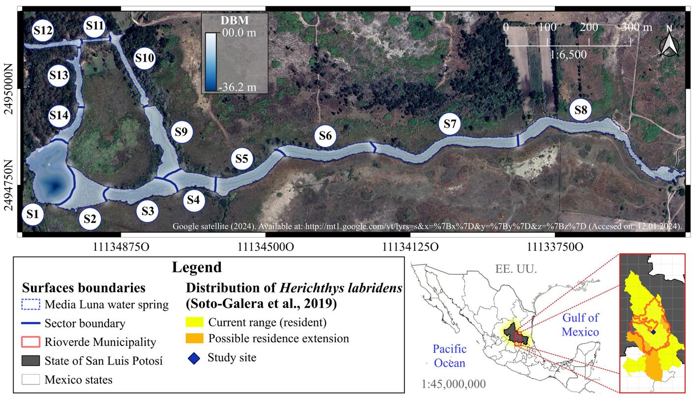
Figure 1. Geographic location, surface area and sectorization (S1 to S14) of the study site Media Luna Spring, San Luis Potosí, Mexico. The 3 main canals started from the set of springs in sector 1 (S1), which correspond to the main lagoon. The Digital Bathymetric Model (DBM) served as the basis for the surface of the system. Sectorization was adapted from Palacio-Núñez et al. (2010). Also, it shows the location of the spring at the country, state, and municipality levels, as well as the recorded range of H. labridens distribution (Soto-Galera et al., 2019). Map by authors.
Specifically, during the summer periods, tourism increases at the study site (Galván-Meza et al., 2018), which influences the distributional range and habitat of H. labridens. Therefore, we obtained spatial records of this species, categorized by adult and juvenile life stages, for summer events of 1999, 2009, and 2019 (Table 1). The databases with spatial and habitat filtering were obtained from 2 sources: for 1999, from Palacio-Núñez et al. (2010), and for the subsequent events, from Rössel-Ramírez, Palacio-Núñez, Martínez-Montoya et al. (2024). These authors recorded each occurrence, by life stage, through direct observation method using snorkeling equipment and a GPS device. Also, to avoid registering the same organism twice in the fieldwork, they validated human observation with subaquatic cameras.
Habitat conditions (e.g., vegetation, bottom types, elevation, and depth) influence the distribution of specialist or endemic species (Naoki et al., 2006). In the present study, we selected 2 predictor variables of the underwater habitat. Due to its relationship with the spatial distribution of various fish communities, the first predictor variable was water depth (McClain & Etter, 2005; Palacio-Núñez et al., 2010; Prchalová et al., 2009; Thrush et al., 2006). The second variable was the underwater coverage, which influences the food and habitat for fish fauna (Brosse & Lek, 2002; Brosse et al., 2007; Rozas & Odum, 1988). Both variables are related to abiotic and biotic factors important for fishes, such as temperature, dissolved oxygen (O2), and biomass (Brandt, 1980; Brosse et al., 1999; Gido & Matthews, 2000; Matthews et al., 2004; Straškraba, 1974).
We obtained a digital bathymetric model for water depth (ranging from 0.0 to -36.2 m) and a raster with reclassification of underwater coverage for the 3 summer events (Rössel-Ramírez et al., 2023). The classification of underwater coverage included the “bare bottom” and “macrophyte vegetation” categories proposed by Palacio-Núñez et al. (2010) and Rössel-Ramírez et al. (2023) for the Media Luna Spring. The bare bottom was classified according to 1) depth, referring to bottom below 12 m, where underwater vegetation does not grow (this type of bottom is only present in S1); 2) tourism, which tends to eliminate vegetation from the sites; and 3) natural process, related to bottom clearings derived from sediment accumulation.
The coverage provided by N. ampla was categorized as follows: 1) small carpet, plants smaller than 0.3 m and with high population density; 2) big carpet, plants with stems of variable length between 0.3 to 2.0 m and large ovoid leaves that overlap; and 3) mature shape, plants with floating and spaced leaves with white flowering. In terms of the presence of remnants of emergent vegetation of the big carpet and mature shape type (S10 to S14), the categories were: big carpet patch and mature shape patch. Thus, a total of 8 coverage categories were included. We loaded both water depth and underwater coverage variables into the geographic projection system WGS 84/Pseudo-Mercator (EPSG: 3857), by the summer event, keeping a Ground Sample Distance of 0.1 m.
We used 2 methods in R® and RStudio® (RStudio Team, 2020) to evaluate both predictor variables in each summer event: the percentage of contribution (Dedman et al., 2017; Freund & Schapire, 1997) via a Gradient Boost Machine (GBM) model (Friedman, 2002), and the Pearson´s correlation to determine the multicollinearity or independence between variables (Guisan & Hofer, 2003). In the first method, this model allows us to estimate the relative contribution of predictor variables as a function of the occurrence of H. labridens (Dedman et al., 2017). For the parameterization, using the GBM package, we selected the Gaussian distribution with a cross-validation of 5,000 repetitions. Also, the model was trained with a random subgroup of training (80%) and testing (20%) from occurrence records (Friedman, 2002; Hijmans, 2012). Additionally, we generated 500 background points to validate the models.
In the 3 summer events, both water depth and underwater coverage had a percentage contribution ≥ 2%, so following the criteria of Awan et al. (2021) and Mohammadi et al. (2021), we selected both for our models (Supplementary material: Figure Sup2.). Subsequently, we evaluated the collinearity of the variables using the Pearson correlation coefficient, avoiding having a high redundancy between variables (Guisan & Hofer, 2003). We established a bivariate correlation below ± 0.70 for the 2 variables, based on a literature review (Awan et al., 2021). As a result, both predictor variables were independent in the 3 events and were included for modeling (Supplementary material: Table Sup2).
Distribution models are a suitable tool for understanding the geographic patterns of species over time (Castillo-Torres et al., 2017; Joy & Death, 2002; Maloney et al., 2013). Carpenter et al. (1993) and Naoki et al. (2006) propose DOMAIN as the appropriate model to project the distribution of endemic species. Therefore, to estimate the distribution of H. labridens, by life stage, we ran this model in Rstudio® for the 3 summer events, loading the water depth and underwater coverage variables and the occurrence records. The packages used were: sp (Pebesma, 2021), dismo, raster, maptools (Hijmans & Elith, 2017), RColorBrewer (Neuwirth, 2014), pander (Farlane, 2013), Rcpp, lattice (Sarkar, 2008), caret (Kuhn et al., 2020), pROC (Robin et al., 2011), and sdm (Naimi & Araujo, 2016).
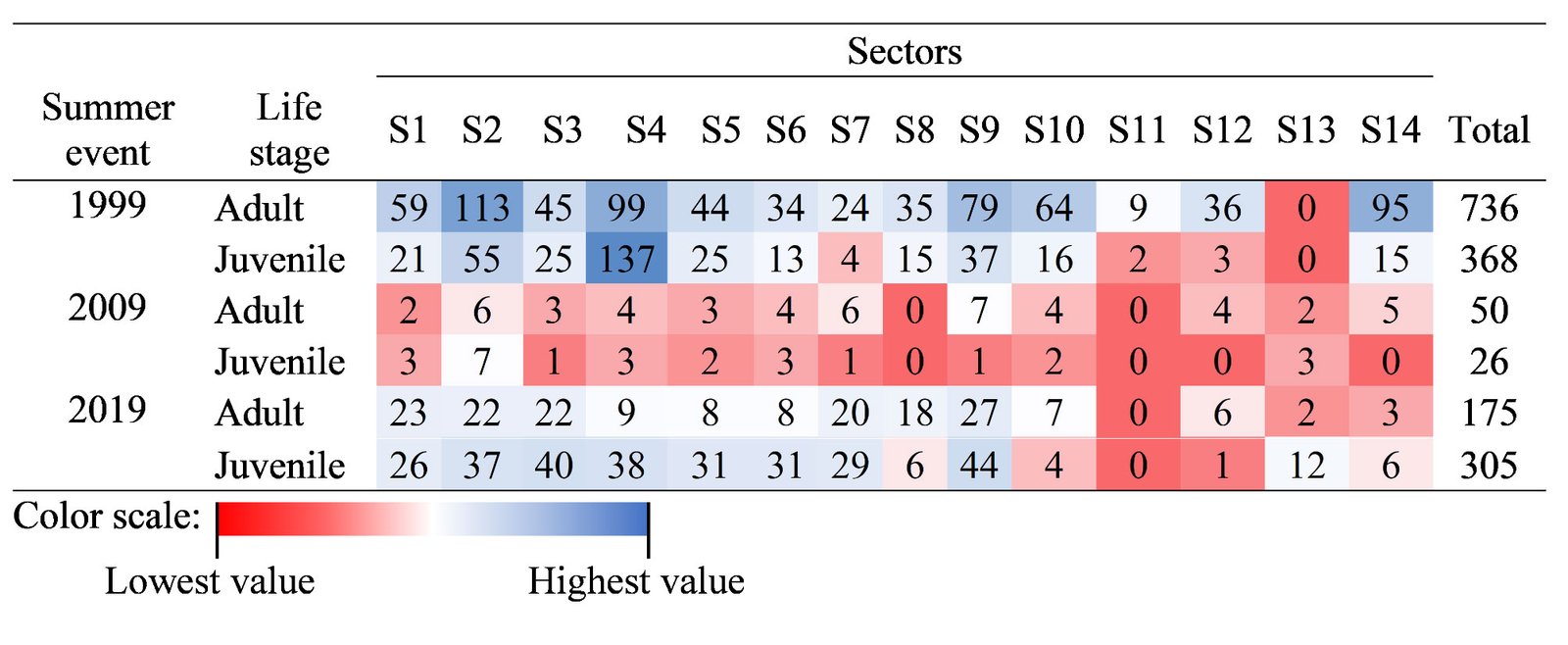
Table 1
Number of occurrence records of H. labridens in the Media Luna spring, San Luis Potosí, Mexico, organized by 3 summer events (years 1999, 2009, and 2019) and life stage (adult and juvenile) in each sector (S1 to S14). The total number of records is included.
Additionally, we generated 500 background points to validate the models; this number was a smaller amount than other studies (e.g., Barbet-Massin et al., 2012) due to the smaller extension of the Media Luna Spring (~7.49 ha). Then, both the occurrences and the background points were subdivided into a training group (80%) and a test group (20%). For modeling, we selected the training groups and the stack containing the variables of water depth and underwater coverage to estimate the DOMAIN probabilistic projections of adult and juvenile stages of H. labridens, in each summer event.
As a last step, we evaluated the prediction performance of each model using the area under the curve (AUC) of the receiver operating characteristic (ROC) curve (Fawcett, 2006). Likewise, we validated the models based on the ROC curve (Fielding & Bell, 1997). The values of the ROC curve were evaluated, following the method of Pearce and Ferrier (2000); according to this method, AUC > 0.5 indicates a model that distinguishes between true presence and absence of a response variable (i.e., occurrence). For partial ROC validation, we followed the Manzanilla-Quiñones (2020) criterion, according to which an AUC ratio value > 1.0 indicates excellent model performance.
The raster layers with spatial distribution probability were loaded into the Qgis® version 3.28.4. We subsequently converted this probability to habitat resistance (Zeller et al., 2012), as a product of the Kernel algorithm, using Equation 1 (Wan et al., 2019):
R = 1000(-1 x SDM)
where R represents the habitat resistance cost assigned to each pixel value and SDM represents the spatial distribution derived from the previously projected models. Additionally, for all raster, the resistance values were rescaled to a range of 0 to 10 by linear interpolation. The minimum resistance (Rmin) was 0 when the distribution probability (DP) was 1, and the maximum resistance (Rmax) was 10 when the DP was 0, following the criterion of Mohammadi et al. (2021).
We calculated the suitability of the core habitat, for H. labridens juveniles and adults, from the accumulation of the habitat resistance cost for the 3 summer events, according to the method of Lawler et al. (2006). This analysis was performed to estimate the accumulation of habitat suitability based on the expected rate of distribution of the species under study (Kaszta et al., 2018).We thus explored the suitable core habitat of H. labridens by life stages.
Based on the habitat resistance (HR) and the new scale of the range of values (i.e., 1 to 10), for both life stages, we categorized the suitable core habitat by quantiles; so that the suitable habitat of the species is better adjusted (Anderson et al., 2003; Burneo et al., 2009). Therefore, we categorized the suitability of the habitat into 3 levels: high (adults, HR ≤ 0.01; juveniles, HR ≤ 0.03), medium (adults, 0.01 < HR ≤ 0.64; juveniles, 0.03 < HR ≤ 1.26); and low (adults, HR > 0.64; juveniles, HR > 1.26). The spatial results were used to identify and regionalize the core area, which was a combination of medium and high suitability for both stages (e.g., Brind’Amour et al., 2005; Poizat & Pont, 1996). Additionally, we calculated the area (ha) per sector of both suitability categories for each sector, by life stage, in the Media Luna Spring.
Results
In terms of the performance of the models, based on the ROC/AUC curve, H. labridens adults had AUCs of 0.67, 0.60, and 0.66 in 1999, 2009, and 2019, respectively; and juveniles had AUCs of 0.73, 0.68, and 0.76 in 1999, 2009, and 2019, respectively (Supplementary material: Figure Sup3). In the validation, all models had a density > 2 of positive cases at a predicted value between 0.6 and 0.9 (Supplementary material: Figure Sup4) in the partial ROC plots. In addition, these models presented a Bandwidth < 0.05 and an AUC ratio > 1.0, per life stage and summer event.
For the adult and juvenile stages of H. labridens, we obtained similar spatial distribution models. In the summer of 1999, the highest probability of distribution (DP > 0.70) was projected in sectors S2-S10; only for adult, the highest probability was too presented in S12. In these sectors, all types of underwater vegetation coverage were present, together with bare bottom by tourism and natural bare bottom; the maximum depth was ~2.5 m. In the following 2 events, the DP > 0.70 was observed only from S2 to S9 which are the sites with the greatest vegetation coverage in big carpet and mature shape (Fig. 2).
Based on the analysis of HR accumulation in adult and juvenile stages, we identified the highest concentration of high and medium suitability (i.e., medium and low categories of cost of resistance) in sectors S2 to S9 (Fig. 3). For the adult stage, high suitability (RH ≤ 0.01) was observed in sectors S2-S4 and S9. For the juvenile stage, high suitability (RH ≤ 0.03) was observed in sectors S2-S9, particularly close to the shores of the spring. Sectors S1 and S10-S14 presented low and medium suitability for both adult and juvenile stages. Sector S1 had the lowest suitability, which represented the highest HR cost for adults (HR > 0.64) and juveniles (HR > 1.26).
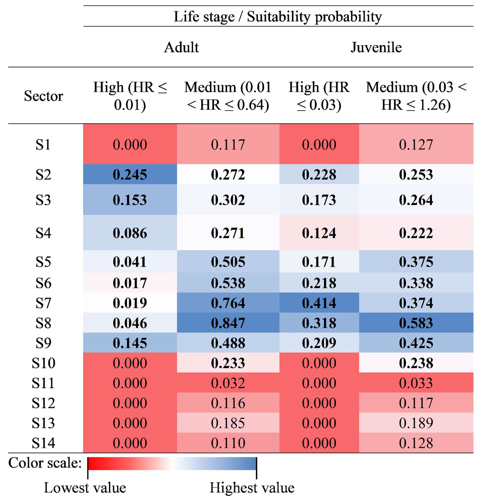
Finally, we calculated the area with high habitat suitability (sectors S2 to S9), with a total area of 0.752 ha for adults and 1.855 ha for juveniles. This represented ~15% and ~36% of the total system extent, respectively. Meanwhile, medium suitability covered an area of 3.987 ha (~ 77%) for adults and 2.834 ha (~ 55%) for juveniles of H. labridens (Table 2). Based on our calculations, the combination of high and medium suitability in sectors S2-S9 covered 4.739 ha for adults and 4.689 ha for juveniles. This represented ~64% of the total area of the spring, now identified as the suitable core habitat for H. labridens. The remaining ~ 36% of the total area of the spring corresponded to sectors S1 and S10-S14, from which ~ 20% corresponded to areas with low habitat suitability in S1 (adults, 1.180 ha; juveniles, 1.169 ha).
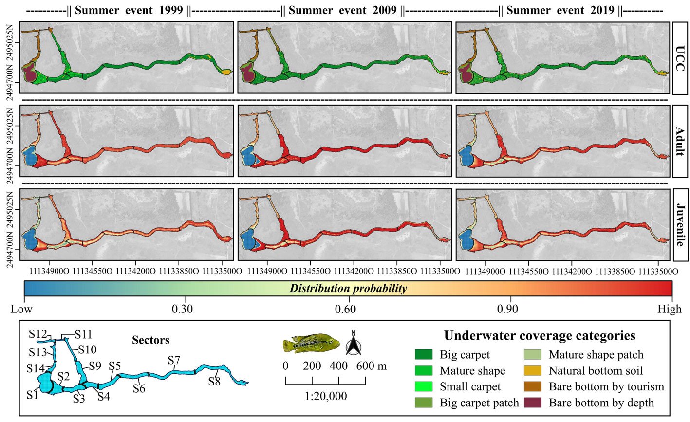
Figure 2. Spatial distribution for the adult and juvenile stages of H. labridens in the summer events of 1999, 2009, and 2019, in the Media Luna Spring, San Luis Potosí, Mexico. It is included in the first row the maps with the underwater coverage composition (UCC), by summer event, for a comparison between habitat changes and variations in the distribution of both life stages. The gradient of distribution probability ranges from low (value = 0) to high (value = 1). Map by authors.
Discussion
We have found that, in the Media Luna Spring, in the 3 summer events assessed, the adult and juvenile stages of H. labridens had a higher probability of distribution (DP > 0.70) in sectors S2-S9, which are characterized by high and medium habitat suitability with depth between ~ 0.5 m and ~ 1.5 m. These observations confirm that this species, like the majority of the Perciformes, have dominant spatial patterns in shallow sites, mainly towards the water edge (McClain & Etter, 2005; Prchalová et al., 2009).
In terms of underwater coverage, for a period of 20 years (1999-2019), both the juvenile and adultstages of H. labridens had a higher preference to sectors with high density of vegetation in the categories big carpet and mature shape. The affinity to vegetated sites is easily understood because it ensures both food and refuge (Rozas & Odum, 1988), especially for juveniles (Artigas-Azas, 2004). Furthermore, in these sectors, there are patches of natural bare bottom, which are important for the reproduction of H. labridens; as has been observed in other cichlids studied (Miller, 1984: Miller et al., 2005). Brandt (1980) found similar conditions on habitat selection and spatial segregation for Perciformes in Lake Michigan, USA. Likewise, Brosse and Lek (2002) reported the assembly of geographic patterns of Eurasian perch (Perca fluviatilis) by habitat affinity in the littoral zone of Lake Pareloup, France.
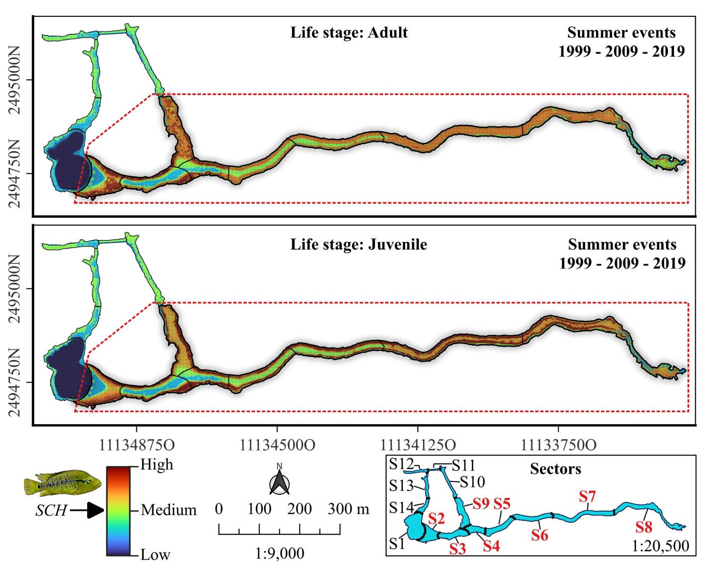
Figure 3. Spatial analysis of suitable core habitat (SCH) for H. labridens at the Media Luna Spring, San Luis Potosí, Mexico. For adult and juvenile stages, each map was generated from the addition of habitat resistance between the 3 summer events (years of 1999, 2009, and 2019). The red dashed contour polygon delineates the region that include the sectors (S2 to S9) with medium- and high-suitability categories, while the outer sectors include the low and medium suitability (S1 and S10 to S14). Map by authors.
In the evaluation of the distribution models by the ROC/AUC curve, Fielding and Bell (1997) and Fawcett (2006) indicate that an AUC > 0.90 represents excellent prediction performance for species distribution models. However, Deshpande (2020) indicates that an AUC between 0.60 and 0.80 constitutes a better prediction classifier, more in line with the ecological reality of the species. Based on this, our models had AUC values ranging from 0.60 to 0.76 for both the adult and juvenile stages in the 3 summer events. We thus conclude that our models had high sensitivity and low specificity, features that correspond to a high discrimination power, in at least ~ 60% of positive cases of occurrence and prediction performance (false positives rate was < 40%). In addition, in the validation by partial ROC, the models had a bandwidth < 0.05 and an AUC ratio > 1.0. Therefore, according to Manzanilla-Quiñones (2020), our models had statistical and ecological significance, across the 3 events of analysis. Thus, we considered that there was a good correlation between habitat variables and the occurrence of H. labridens to allow accurate modeling of its spatial distribution.
Table 2
Area (ha) by suitability category (medium and high) of the core habitat for H. labridens adults and juveniles in the Media Luna Spring, San Luis Potosí, Mexico. The area was calculated for each one from 14 sectors. The values in bold denote the greatest area occupied based on the suitability probability. In most cases, the greatest and most representative areas were between sectors S2 and S9.
Our DOMAIN models provided a good overview of the variation in the spatial distribution of the endemic H. labridens, in both life stages. In addition to that, previous work (Hirzel et al., 2006; Zeller et al., 2012) indicates that estimating core habitats is more accurate when work is carried out over long temporal scales, because it was possible to discern between low, medium, and high resistance habitat, according to the relevant variables (Lawler et al., 2006). Following this, our maps and tables of the suitable core habitat for H. labridens were more conclusive in quantifying its cost of resistance according to the variables of water depth and underwater coverage. We confirmed that the sectors S2-S9 represent the suitable core habitat for H. labridens in the adult and juvenile stages for 20 years at least. These sectors presented low-cost resistance values (i.e., high suitability of core habitat) in adults (RH < 0.01) and juveniles (RH < 0.03), especially towards the shores of the spring, where the maximum depth was ~ 1.5 m and the underwater vegetation coverage was big carpet and mature shape.
It should be noted that the Media Luna Spring has been modified by tourism (Damián-Santiago, 2015; Galván-Meza et al., 2018), causing changes in the composition of underwater coverage for over 2 decades. This was reflected in the progressive decrease in vegetation coverage, although the depth was not noticeably affected, where more than 90% of the spring surface area maintained a depth of less than 3.5 m (pers. obs.). Thus, the distribution area and core habitat, as well as a higher number of occurrences, from S2 to S9 for both adult and juvenile stages, is likely related to habitat degradation in tourism sectors, as has happened in other sites (Hickley et al., 2004; Miranda et al., 2010). Particularly, 2009 was a critical year due to habitat pressure from tourism (Chávez, 2016), linked to the drastic decrease in occurrences for both life stages. Despite this habitat pressure, this speciessurvives and reproduces in this water system, but in a suboptimal population state. Therefore, it is important to keep H. labridens under the category of endangered species as a conservation measure (Miranda et al., 2009).
In conclusion, we found that the suitable core habitat for H. labridens in Media Luna Spring is the region between S2 and S9, which is characterized by a combination of shallow sites associated with dense coverage of emergent, sub-emergent, and floating vegetation patches. It is important to note that these coverage combinations provide resources for feeding and habitat refuge. This information, obtained on a temporal scale, is important to increase our knowledge about the variation in spatial distribution and core habitat of this endemic and threatened species. With this, it is now possible to compare and associate occurrence records with changes in vegetation coverage or anthropogenic pressure. Based on our findings, we urgently propose establishing this estimated core habitat (sectors S2-S9) as a priority conservation area for H. labridens. This means that these sectors, located in the eastern region of the spring, should be adequately managed without eliminating vegetation or modifying the natural system. Meanwhile, Sectors S1 and S10 to S14 would be categorized as suitable for tourism use, with management and monitoring by the local authorities and ejido leaders at the site.
In addition, we consider that our study provides relevant information on the abundance and habitat preferences of H. labridens to update the management plan and implement habitat care campaigns for the Media Luna Spring. At the same time, to include reports for other endemic species in this spring, as A. toweri (Rössel-Ramírez, Palacio-Núñez, Espinosa et al., 2024). Taken together, our spatial results reinforce the importance of identifying conservation areas or regions in this semi-arid spring.
Acknowledgments
We thank Jesús Enríquez for their participation in fieldwork during the sampling events. In addition, we thank to the Secretaría de Ecología y Gestión Ambiental (Segam; Oficio: ECO.05.1068), the local authorities of Rioverde municipality, and the Jabalí ejido council for allowing us to carry out this study in the Media Luna Spring.
References
Anderson, R. P., Lew, D., & Peterson, A. T. (2003). Evaluating predictive models of species’ distributions: criteria for selecting optimal models. Ecological Modelling, 162, 211–232. https://doi.org/10.1016/S0304-3800(02)00349-6
Artigas-Azas, J. M. 2004). “Herichthys labridens (Pellegrin, 1903)”. Cichlid Room Companion. Retrieved on January 1rst, 2024 from: https://cichlidae.com/species.php?id=209&lang=es. (crc10342)
Awan, M. N., Saqib, Z., Buner, F., Lee, D. C., & Pervez, A. (2021). Using ensemble modeling to predict breeding habitat of the red-listed Western Tragopan (Tragopan melanocephalus) in the Western Himalayas of Pakistan. Global Ecology and Conservation, 31, e01864. https://doi.org/10.1016/j.gecco.2021.e01864
Barbet-Massin, M., Jiguet, F., Albert, C. H., & Thuiller, W. (2012). Selecting pseudo-absences for species distribution models: how, where and how many? Methods in Ecology and Evolution, 3, 327–338. https://doi.org/10.1111/j.2041-210x.2011.00172.x
Brandt, S. B. (1980). Spatial segregation of adult and young-of-the-year alewives across a thermocline in Lake Michigan. Transactions of the American Fisheries Society, 109, 469–478. https://doi.org/10.1577/1548-8659(1980)109<469:SSOAAY>2.0.CO;2
Brind’Amour, A., Boisclair, D., Legendre, P., & Borcard, D. (2005). Multiscale spatial distribution of a littoral fish community in relation to environmental variables. Limnology and Oceanography, 50, 465–479. https://doi.org/10.4319/lo.2005.50.2.0465
Brosse, S., Grossman, G. D., & Lek, S. (2007). Fish assemblage patterns in the littoral zone of a European reservoir. Freshwater Biology, 52, 448–458. https://doi.org/10.1111/j.1365-2427.2006.01704.x
Brosse, S., & Lek, S. (2002). Relationships between environmental characteristics and the density of age-0 Eurasian perch Perca fluviatilis in the littoral zone of a lake: a nonlinear approach. Transactions of the American Fisheries Society, 131, 1033–1043. http://dx.doi.org/10.1577/1548-8659(2002)131<1033:RBECAT>2.0.CO;2
Brosse, S., Lek, S., & Dauba, F. (1999). Predicting fish distribution in a mesotrophic lake by hydroacoustic survey and artificial neural networks. Limnology and Oceanography, 44, 1293–1303. https://doi.org/10.4319/lo.1999.44.5.1293
Burneo, S., González-Maya, J. F., & Tirira, D. (2009). Distribution and habitat modelling for Colombian weasel Mustela felipei in the Northern Andes. Small Carnivore Conservation, 41, 41–45.
Castillo-Torres, P. A., Martínez-Meyer, E., Córdova-Tapia, F., & Zambrano, L. (2017). Potential distribution of native freshwater fish in Tabasco, Mexico. Revista Mexicana de Biodiversidad, 88, 415–424. https://doi.org/10.1016/j.rmb.2017.03.001
Carpenter, G., Gillison, A. N., & Winter, J. (1993). DOMAIN: a flexible modelling procedure for mapping potential distributions of plants and animals. Biodiversity & Conservation, 2, 667–680.
Ceballos, G., Pardo, E. D., Estévez, L. M., & Pérez, H. E. (2018). Los peces dulceacuícolas de México en peligro de extinción. Fondo de Cultura Económica. Cd. de México.
Chávez, M. G. G. (2016). El impacto del turismo en la conservación de la biodiversidad en San Luis Potosí. Sociedad y Ambiente, 11, 148–159.
Contreras-Balderas, S. (1969). Perspectivas de la ictiofauna en las zonas áridas del norte de México. In Simposium Internacional sobre Aumento de Producción de Alimentos en Zonas Áridas. Centro Internacional de Estudios sobre Tierras Áridas, Universidad de Texas Tech.
Contreras-MacBeath, T., Rodríguez, M. B., Sorani, V., Goldspink, C., & Reid, G. M. (2014). Richness and endemism of the freshwater fishes of Mexico. Journal of Threatened Taxa, 6, 5421–5433. https://doi.org/10.11609/JoTT.o3633.5421-33
Damián-Santiago, F. I. (2015). Caracterización del perfil del ecoturista que visita el Parque Estatal Manantial de la Media Luna, en el Ejido El Jabalí, municipio de Rioverde, San Luis Potosí, México (Bachelor’s Thesis). Departamento Forestal, Universidad Autónoma Agraria Antonio Narro. Saltillo, Coahuila, México.
Dedman, S., Officer, R., Clarke, M., Reid, D. G., & Brophy, D. (2017). Gbm. auto: a software tool to simplify spatial modelling and Marine Protected Area planning. Plos One, 12, e0188955. https://doi.org/10.1371/journal.pone.0188955
De la Vega-Salazar, M. Y. (2003). Situación de los peces dulceacuícolas en México. Ciencias, 72, 20–30.
Deshpande, R. (2020). ROC Curve and AUC in Machine learning and R pROC Package. Retrieved on September 08th, 2023 from: https://medium.com/swlh/roc-curve-and-auc-detailed-understanding-and-r-proc-package-86d1430a3191
Dudgeon, D., Arthington, A. H., Gessner, M. O., Kawabata, Z. I., Knowler, D. J., Lévêque, C. et al. (2005). Freshwater biodiversity: importance, threats, status and conservation challenges. Biological Reviews, 81, 163. https://doi.org/10.1017/s1464793105006950
Eby, L. A., Fagan, W. F., & Minckley, W. L. (2003). Variability and dynamics of a desert stream community. Ecological Applications, 13, 1566–1579. https://doi.org/10.1890/02-5211
Elith, J., & Leathwick, J. R. (2009). Species distribution models: ecological explanation and prediction across space and time. Annual Review of Ecology, Evolution, and Systematics, 40, 677–697. https://doi.org/10.1146/annurev.ecolsys.110308.120159
Farlane, J. M. (2013). Pandoc User’s Guide. Accessed on RStudio: Integrated Development for R. RStudio, PBC, Boston, MA URL: http://www.rstudio.com/
Fawcett, T. (2006). An introduction to ROC analysis. Pattern Recognition Letters, 27, 861–874. https://doi.org/10.1016/j.patrec.2005.10.010
Fielding, A. H., & Bell, J. F. (1997). A review of methods for the assessment of prediction errors in conservation presence/absence models. Environmental Conservation, 24, 38–49.
Freund, Y., & Schapire, R. E. (1997). A decision-theoretic generalization of on-line learning and an application to boosting. Journal of Computer and System Sciences, 55, 119–139. https://doi.org/10.1006/jcss.1997.1504
Friedman, J. H. (2002). Stochastic gradient boosting. Computational Statistics and Data Analysis, 38, 367–378. https://doi.org/10.1016/S0167-9473(01)00065-2
Galván-Meza, C. J., Flores-Castillo, E., Espericueta-Bocanegra, E. D., & Gutiérrez-Pérez, M. G. (2018). Análisis del impacto multidisciplinar del turismo dentro del ejido El Jabalí – Media Luna – San Luis Potosí. Medio Ambiente, Sustentabilidad y Vulnerabilidad Social, 5, 419–434.
Gido, K. B., & Matthews, W. J. (2000). Dynamics of the offshore fish assemblage in a southwestern reservoir (Lake Texoma, Oklahoma-Texas). Copeia, 2000, 917–930. http://dx.doi.org/10.1643/0045-8511(2000)000[0917:DOTOFA]2.0.CO;2
Guisan, A., & Hofer, U. (2003). Predicting reptile distributions at the mesoscale: relation to climate and topography. Journal of Biogeography, 30, 1233–1243. https://doi.org/10.1046/j.1365-2699.2003.00914.x
Hickley, P., Muchiri, M., Boar, R., Britton, R., Adams, C., Gichuru, N. et al. (2004). Habitat degradation and subsequent fishery collapse in Lakes Naivasha and Baringo, Kenya. International Journal of Ecohydrology & Hydrobiology, 4, 503–517. http://karuspace.karu.ac.ke/handle/20.500.12092/1918
Hijmans, R. J. (2012). Cross-validation of species distribution models: removing spatial sorting bias and calibration with a null model. Ecology, 93, 679–688. https://doi.org/10.1890/11-0826.1
Hijmans, R. J., & Elith, J. (2017). Species distribution modeling with R. R CRAN Project. https://www.researchgate.net/file.PostFileLoader.html?id=5730d34496b7e4bb46356f31&assetKey=AS%3A359897272209410%401462817604682
Hirzel, A. H., Le Lay, G., Helfer, V., Randin, C., & Guisan, A. (2006). Evaluating the ability of habitat suitability models to predict species presences. Ecological Modelling, 199, 142–152. https://doi.org/10.1016/j.ecolmodel.2006.05.017
IUCN (International Union for Conservation of Nature). (Version 2024.2). The IUCN red list of threatened species. Retrieved on January 25th, 2024 from: https://www.iucnredlist.org/
Joy, M. K., & Death, R. G. (2002). Predictive modelling of freshwater fish as a biomonitoring tool in New Zealand. Freshwater Biology, 47, 2261–2275. https://doi.org/10.1046/j.1365-2427.2002.00954.x
Kaszta, Ż., Cushman, S. A., Sillero-Zubiri, C., Wolff, E., & Marino, J. (2018). Where buffalo and cattle meet: modelling interspecific contact risk using cumulative resistant kernels. Ecography, 41, 1616–1626. https://doi.org/10.1111/ecog.03039
Kuhn, M., Wing, J., Weston, S., Williams, A., Keefer, C., Engelhardt, A. et al. (2020). Package ‘caret’: classification and regression training, R-package version 6.0-p. Misc Functions for Training and Plotting Classification and Regression Models.
Lawler, J. J., White, D., Neilson, R. P., & Blaustein, A. R. (2006). Predicting climate-induced range shifts: model differences and model reliability. Global Change Biology, 12, 1568–1584. https://doi.org/10.1111/j.1365-2486.2006.01191.x
Lozano-Vilano, M. L., Contreras-Balderas, A. J., Ruiz-Campos, G., & García-Ramírez, M. E. (2021). Current conservation status of some freshwater species and their habitats in México. In D. L. Propst, J. E, Williams, K. R. Bestgen, & C. W. Hoagstrom (Eds.), Standing between life and extinction: ethics and ecology of conserving aquatic species in North American deserts (pp. 79–88). Chicago: The University of Chicago Press.
Macías-Andrade, M. E., & Maldonado-González, D. P. (2011). La práctica ecoturística en el Parque Estatal de la Media Luna en Rioverde SLP (Tesis). Facultad de Economía, Universidad Autónoma de San Luis Potosí. San Luis Potosí, México.
Maloney, K. O., Weller, D. E., Michaelson, D. E., & Ciccotto, P. J. (2013). Species distribution models of freshwater stream fishes in Maryland and their implications for management. Environmental Modeling & Assessment, 18, 1–12. https://doi.org/10.1007/s10666-012-9325-3
Manzanilla-Quiñones, U. (2020). Validación de modelos de distribución con ayuda de la plataforma niche toolbox de Conabio. Retrieved on June 29th, 2023 from: https://www.researchgate.net/publication/341820933
Matthews, W. J., Gido, K. B., & Gelwick, F. P. (2004). Fish assemblages of reservoirs, illustrated by Lake Texoma (Oklahoma-Texas, USA) as a representative system. Lake and Reservoir Management, 20, 219–239. https://doi.org/10.1080/07438140409354246.
Menke, K. (2019). Discover QGIS 3. x. Locate Press.
McClain, C. R., & Etter, R. J. (2005). Mid-domain models as predictors of species diversity patterns: bathymetric diversity gradients in the deep sea. Oikos, 109, 555–566. https://doi.org/10.1111/j.0030-1299.2005.13529.x
Miller, R. R. (1984). La Media Luna, San Luis Potosí, at edge of Chihuahua Desert, México. In Proceedings of the Desert Fishes Council Co. (Ed.). Volumes XVI-XVIII. Annual Symposium Bishop, CA. 67–72.
Miller, R. R., Minckley, W. L., Norris, S. M., & Gach, M. H. (2005). Freshwater fishes of Mexico (Núm. QL 629. M54 2005). Chicago: University of Chicago Press.
Miranda, L. E., Spickard, M., Dunn, T., Webb, K. M., Aycock, J. N., & Hunt, K. (2010). Fish habitat degradation in US reservoirs. Fisheries, 35, 175–184. https://doi.org/10.1577/1548-8446-35.4.175
Miranda, R., Monks, S., Galicia, D., & Pulido-Flores, G. (2009). Threatened fishes of the world: Herichthys labridens (Pellegrin, 1903). Environmental Biology of Fishes, 86, 377. https://doi.org/10.1007/s10641-009-9528-x
Mohammadi, A., Almasieh, K., Nayeri, D., Ataei, F., Khani, A., López-Bao, J. V. et al. (2021). Identifying priority core habitats and corridors for effective conservation of brown bears in Iran. Scientific Reports, 11, 1044. https://doi.org/10.1038/s41598-020-79970-z
Naimi, B., & Araujo, M. B. (2016). sdm: a reproducible and extensible R platform for species distribution modelling. Ecography, 39, 368–375. https://doi.org/10.1111/ecog.01881
Naoki, K., Gómez, M. I., López, R. P., Meneses, R. I., & Vargas, J. (2006). Comparación de modelos de distribución de especies para predecir la distribución potencial de vida silvestre en Bolivia. Ecología en Bolivia, 41, 65–78.
Neuwirth, E. (2014). RColorBrewer: ColorBrewer palettes. R package version 1.1-2. The R Foundation.
Palacio-Núñez, J. (2007). Designación de zonas prioritarias de conservación en el Parque Estatal de la Media Luna (México): utilización de aves y peces como bioindicadores (Ph.D. Thesis). Instituto de Investigación de la Biodiversidad (CIBIO), Universidad de Alicante. Alicante, España.
Palacio-Núñez, J., Olmos-Oropeza, G., Verdú, J. R., Galante, E., Rosas-Rosas, O. C., Martínez-Montoya, J. F. et al. (2010). Traslape espacial de la comunidad de peces dulceacuícolas diurnos en el sistema de humedal Media Luna, Rioverde, SLP, México. Hidrobiológica, 20, 21–30.
Palacio-Núñez, J., Martínez-Montoya, J. F., Olmos-Oropeza, G., Martínez-Calderas, J. M., Clemente-Sánchez, F., & Enríquez, J. (2015). Distribución poblacional y abundancia de los peces endémicos de la Llanura de Rioverde, SLP, México. Agroproductividad, 8, 17–24.
Pearce, J., & Ferrier, S. (2000). Evaluating the predictive performance of habitat models developed using logistic regression. Ecological Modelling, 133, 225–245. https://doi.org/10.1016/S0304-3800(00)00322-7
Pebesma, E. (2021). Map overlay and spatial aggregation in sp, Report 253. Institute for Geoinformatics. University of Muenster, Weseler Strasse.
Pellegrin, J. (1903). Description de Cichlidés nouveax de la collection du Muséum. Bulletin du Musée National d’Histoire Naturelle, 9, 120–125.
Periódico Oficial del gobierno del estado libre y soberano de San Luis Potosí (07 de junio de 2003). Declaración de Área Natural Protegida bajo la modalidad de “Parque Estatal” denominado “Manantial de la Media Luna”. Retrieved on October 07th, 2023 from: http://201.144.107.246/InfPubEstatal2/_SECRETAR%C3%8DA%20DE%20ECOLOG%C3%8DA%20Y%20GESTI%C3%93N%20AMBIENTAL/Art%C3%ADculo%2018.%20fracc.%20II/Normatividad/Decretos/Decreto%20Media%20Luna.pdf. Secretaría General de Gobierno, 2–12.
Poizat, G., & Pont, D. (1996). Multi-scale approach to species–habitat relationships: juvenile fish in a large river section. Freshwater Biology, 36, 611–622. https://doi.org/10.1046/j.1365-2427.1996.00129.x
Prchalová, M., Kubečka, J., Čech, M., Frouzová, J., Draštík, V., Hohausová, E. et al. (2009). The effect of depth, distance from dam and habitat on spatial distribution of fish in an artificial reservoir. Ecology of Freshwater Fish, 18, 247–260. https://doi.org/10.1111/j.1600-0633.2008.00342.x
Ricciardi, A., & Rasmussen, J. B. (1999). Extinction rates of North American freshwater fauna. Conservation Biology, 13, 1220–1222. https://doi.org/10.1046/j.1523-1739.1999.98380.x
Robin, X., Turck, N., Hainard, A., Tiberti, N., Lisacek, F., Sánchez, J. et al. (2011). “pROC: an open-source package for R and S+ to analyze and compare ROC curves”. BMC Bioinformatics, 12, 1–77. https://doi.org/10.1186/1471-2105-12-77
Rössel-Ramírez, D. W., Palacio-Núñez, J., Espinosa, S., & Martínez-Montoya, J. F. (2023). Raster layers of underwater coverage and water depth of the Media Luna spring, Mexico, generated from data from three summer periods (in the years 1999, 2009, and 2019). Zenodo. https://doi.org/10.5281/zenodo.10253601
Rössel-Ramírez, D. W., Palacio-Núñez, J., Martínez-Montoya, J. F., & Espinosa, S. (2024). Occurrences records of Herichthys labridens (Cichliformes: Cichlidae), with associated habitat information, in the Media Luna spring, San Luis Potosí, Mexico (Version 1) [Data set]. Zenodo. https://doi.org/10.5281/zenodo.14231104
Rössel-Ramírez, D. W., Palacio-Núñez, J., Espinosa, S., & Martínez-Montoya, J. F. (2024). Temporal variation in the relative abundance, suitable habitat selection, and distribution of Ataeniobius toweri (Meek, 1904) (Goodeidae), by life stages, in the Media Luna spring, Mexico. Environmental Biology of Fishes, 107, 173–188. https://doi.org/10.1007/s10641-024-01520-7
Rozas, L. P., & Odum, W. E. (1988). Occupation of submerged aquatic vegetation by fishes: testing the roles of food and refuge. Oecologia, 77, 101–106. https://www.jstor.org/stable/4218746
RStudio Team (2020). RStudio: Integrated Development for R. RStudio, PBC, Boston, MA URL: http://www.rstudio.com/
Ruetz III, C. R., Trexler, J. C., Jordan, F., Loftus, W. F., & Perry, S. A. (2005). Population dynamics of wetland fishes: spatio-temporal patterns synchronized by hydrological disturbance? Journal of Animal Ecology, 74, 322–332. https://doi.org/10.1111/j.1365-2656.2005.00926.x
Ruiz-Campos, G., Camarena-Rosales, F., Contreras-Balderas, S., Reyes-Valdez, C. A., De La Cruz-Agüero, J., & Torres-Balcázar, E. (2006). Distribution and abundance of the endangered killifish, Fundulus lima (Teleostei: Fundulidae), in oases of central Baja California Peninsula, Mexico. The Southwestern Naturalist, 51, 502–509.
Salazar, H. C., Sáenz, E. O., & Rivera, J. R. A. (2002). Agua de riego en la región de Rioverde, San Luis Potosí, México. Tecnología y Ciencias del Agua, 17, 37–56.
Sarkar, D. (2008). lattice: multivariate data visualization with R. Springer-Verlag, New York. http://lmdvr.r-forge.r-project.org/
Segam (Secretaría de Ecología y Gestión Ambiental). (2019). Declaratoria de Área Natural Protegida bajo la modalidad de Parque Estatal denominado “Manantial de la Media Luna”. Diario Oficial de San Luis Potosí. 7 de junio del 2003. Retrieved on May 12th, 2019 from: www.segam.gob.mx
Soto-Galera, E., Mejía-Guerrero, O., & Pérez-Miranda, F. (2019). Herichthys labridens. The IUCN Red List of Threatened Species 2019: e.T192897A2179729. Retrieved on 04 December 2023 from: http://dx.doi.org/10.2305/IUCN.UK.2019-2.RLTS.T192897A2179729
Straškraba, M. (1974). Seasonal cycle of the depth distribution of fish in the Klıcava Reservoir. Czech Journal of Animal Sciences, 19, 656–660.
Thrush, S., Dayton, P., Cattaneo-Vietti, R., Chiantore, M., Cummings, V., Andrew, N. et al. (2006). Broad-scale factors influencing the biodiversity of coastal benthic communities of the Ross Sea. Deep Sea Research Part II: Topical Studies in Oceanography, 53, 959–971. https://doi.org/10.1016/j.dsr2.2006.02.006
Torres-Orozco, R. E., & Pérez-Hernández, M. A. (2011). Los peces de México: una riqueza amenazada. Revista Digital Universitaria, 12, 1–15.
Wan, H. Y., Cushman, S. A., & Ganey, J. L. (2019). Improving habitat and connectivity model predictions with multi-scale resource selection functions from two geographic areas. Landscape Ecology, 34, 503–519. https://doi.org/10.1007/s10980-019-00788-w
Wiersema, J. H., Novelo, A. R., & Bonilla-Barbosa, J. R. (2008). Taxonomy and typification of Nymphaea ampla (Salisb.) DC. sensu lato (Nymphaeaceae). Taxon, 57, 967–974. https://doi.org/10.1002/tax.573025
Zeller, K. A., McGarigal, K., & Whiteley, A. R. (2012). Estimating landscape resistance to movement: a review. Landscape Ecology, 27, 777–797. https://doi.org/10.1007/s10980-012-9737-0

Conservadurismo de nicho ecológico de algunas especies hermanas del género Euglossa (Apidae: Euglossini) en México y Centroamérica
Ecological niche conservatism in sister species of Euglossa (Apidae: Euglossini) from Mexico and Central America
A. Celeste Martínez-Cervantes, Enrique Martínez-Meyer e Ismael A. Hinojosa-Díaz *
Universidad Nacional Autónoma de México, Instituto de Biología, Departamento de Zoología, Tercer Circuito Universitario s/n, Ciudad Universitaria, Coyoacán, 04510 Ciudad de México, México
*Autor para correspondencia: ihinojosa@ib.unam.mx (I.A. Hinojosa-Díaz)
Recibido: 10 enero 2025; aceptado: 30 octubre 2025
Resumen
Las abejas de la tribu Euglossini son un grupo importante de polinizadores de la región neotropical al contribuir a la reproducción de plantas por las visitas de las hembras en búsqueda de recursos florales, mientras los machos son polinizadores específicos de grupos de orquídeas en su búsqueda de químicos aromáticos, que pueden obtener de otros sustratos y que son utilizados como señales de apareamiento. El género Euglossa es el más diverso de la tribu, ocupa diversos ambientes desde el norte de México hasta el sur de la región neotropical. Se conocen las afinidades filogenéticas de muchas de las especies del género. En este estudio se describe y compara el nicho climático en 3 pares de especies hermanas del género Euglossa bajo la premisa de conservadurismo de nicho, encontrando similitud significativa solo entre las especies hermanas dentro del subgénero Euglossa, mientras que en los otros pares de especies comparadas, la similitud de nicho está más relacionada con la simpatría de las especies que con la cercanía filogenética.
Palabras clave: Abejas de orquídeas; Conservadurismo de nicho; Simpatría
Abstract
Bees of the tribe Euglossini are important pollinators in the Neotropical region contributing to the reproduction of a variety of plants visited by females in search for floral resources while males are specialized pollinators of groups of orchids in their quest for aromatic chemicals, also retrieved from other sources and later used as sexual signals. Euglossa is the most diverse genus in the tribe ranging from northern Mexico to the southern parts of the Neotropical region. General phylogenetic affinities are known for several species in the genus. Here we describe and compare the ecological niche for 3 pairs of sister species of the genus Euglossa under the premise of niche conservatism, for which we found significant similarity only between sister species in the subgenus Euglossa, whereas in the other comparisons niche similarity is explained by the sympatric distributions of the species rather than by their phylogenetic relationships.
Keywords: Orchid bees; Niche conservatism; Sympatry
Introducción
Las abejas de las orquídeas suelen exhibir colores metálicos brillantes y partes bucales alargadas, que en ciertas especies puede superar la longitud de sus propios cuerpos (Engel y Rasmussen, 2020; Roubik y Hanson, 2004). Los machos, se distinguen por una serie de caracteres sexuales secundarios relacionados con la recolección de sustancias aromáticas, sobresale la tibia posterior ancha donde se almacenan estos químicos combinados con secreciones de las glándulas labiales (Engel y Rasmussen, 2020; Roubik y Hanson, 2004). Estos compuestos funcionan como señales de atracción y estimulación de las hembras para el apareamiento (Henske et al., 2023). Los machos adquieren compuestos aromáticos principalmente de orquídeas, aunque también frecuentan otras familias de plantas y otros recursos como madera en descomposición, hongos e incluso productos químicos sintéticos (Engel y Rasmussen, 2020; Roubik y Hanson, 2004). Estas abejas representan uno de los principales polinizadores del Neotrópico al participar en la polinización de más de 60 familias de plantas, incluyendo alrededor de 700 especies de orquídeas (Roubik y Hanson, 2004).
La tribu Euglossini se originó entre hace 27 y 42 millones de años en América del Sur (Ramírez et al., 2010; Roubik y Hanson, 2004). Se han propuesto varias hipótesis con respecto a las relaciones entre los géneros, tanto con caracteres moleculares como morfológicos (Ramírez et al., 2010). Actualmente, se han registrado 249 especies de euglossinos exclusivamente neotropicales (Engel y Rasmussen, 2020), divididos en 5 géneros: Aglae, Exaerete, Eulaema, Eufriesea y Euglossa.
El género Euglossa es el más diverso dentro de la tribu, con 139 especies (Engel y Rasmussen, 2020). Su origen se remonta al Mioceno medio (Ramírez et al., 2010). Las relaciones dentro del género no están del todo resueltas y varios autores han subdividido al género en 6 subgéneros: Alloglossura, Dasystilbe, Euglossella, Euglossa, Glossurella y Glossuropoda. Recientemente, se han propuesto 4 nuevos subgéneros: Eurhytisma, Glossurodes, Parisoglossa y Trachyglossa para ayudar a resolver la parafilia de los subgéneros Glossurella y Glossuropoda (Engel, 2021).
Las relaciones evolutivas entre las especies o diferentes taxones se muestran a través de las filogenias (Eliosa et al., 2010). En los árboles filogenéticos podemos observar gráficamente estas relaciones y entender de mejor manera las conexiones entre las especies o los taxones. El conservadurismo de nicho es la tendencia de las especies a retener características ecológicas en el tiempo cuando se enfrentan a condiciones ambientales nuevas (Wiens y Donoghue, 2004; Wiens y Graham, 2005). El conservadurismo de nicho tiende a romperse con el tiempo, lo que resulta en un mayor conservadurismo entre especies que han divergido recientemente y que están estrechamente relacionadas, como es el caso de las especies hermanas (Pyron et al., 2015).
En este trabajo se describe y compara el nicho climático de especies hermanas de Euglossa, incluyendo los subgéneros Euglossa (sensu stricto), Dasystilbe y Eurhytisma para evaluar qué tan conservados son los nichos entre y dentro de estos subgéneros. Bajo la premisa del conservadurismo de nicho ecológico, esperamos que los nichos de las especies dentro de los subgéneros sean más parecidos que entre especies de subgéneros distintos.
Materiales y métodos
Especies
Subgénero Euglossa s. st. Euglossa dilemma y E. viridissima son especies hermanas distintivas dentro del subgénero Euglossa y muy afines morfológicamente que divergieron hace ~ 150,000 años (Brand et al., 2020; Eltz et al., 2011). Antes de la descripción de Euglossa dilemma (Eltz et al., 2011), E. viridissima se consideraba una especie con variación morfológica, hasta que se demostró inicialmente con evidencia morfológica y distribucional (Eltz et al., 2011), y reforzándose con evidencia genética que E. dilemma es una especie distinta (Brand et al., 2020). Ambas especies presentan poblaciones simpátricas, con áreas de traslape al sur-sureste de México y parte de Guatemala y Belice.
El subgénero Dasystilbe solo cuenta con 2 especies: E. obrima y E. villosa. Son abejas grandes que miden ~ 15 mm de longitud, presentan una coloración verde metálico con iridiscencia azul o bronce. Su cuerpo está cubierto de sedas largas y densas, especialmente en los costados (Hinojosa-Díaz et al., 2011). Los machos presentan una mandíbula bidentada, mientras que las hembras una tridentada (Hinojosa-Díaz et al., 2011).
Subgénero Eurhytisma (antes parte de Glossurella). El subgénero Glossurella era considerado un grupo parafilético (Engel, 2021); sin embargo, la relación de especies hermanas entre E. obtusa y E. dodsoni se ha mantenido a lo largo de las filogenias realizadas del género (Ghassemi-Khademi, 2018; Ramírez et al., 2010). Más tarde, se describe la especie E. williamsi, la cual no ha sido considerada en la metodología de las filogenias del género; no obstante, en el artículo donde se describe la especie se señala que ésta, muy probablemente, conforma un grupo monofilético junto con E. obtusa y E. dodsoni al presentar estructuras morfológicas similares, como la presencia de la mancha preomaular (en el mesepisterno) compartida entre las 3 especies (Hinojosa-Díaz y Engel, 2011). Partiendo de esta idea, Engel (2021) une a estas 3 especies en un nuevo subgénero llamado Eurhytisma. Lamentablemente, debido a la falta de registros de la especie E. williamsi, se decidió omitirla del presente estudio, sin embargo, la fuerte afinidad morfológica entre E. obtusa y E. dodsoni es un argumento fuerte para considerarlas más cercanas entre ellas respecto de E. williamsi (Hinojosa-Díaz y Engel, 2011).
Los datos recopilados se obtuvieron de diversas fuentes, incluyendo colecciones biológicas y acervos electrónicos: Colección Nacional de Insectos del Instituto de Biología de la Universidad Nacional Autónoma de México (CNIN); base de datos de la Colección de abejas de ECOSUR en San Cristóbal de las Casas, México; Sistema Nacional de Información sobre Biodiversidad de México (Conabio, 2021); Global Biodiversity Information Facility (GBIF); Discover Life (Ascher y Pickering, 2018) y Catalogue of Bees (Hymenoptera, Apoidea) in the Neotropical Region (Moure y Melo, 2023). Posteriormente, se depuraron los datos eliminando registros duplicados y se georreferenciaron aquellos sin coordenadas mediante el uso de Google Earth (tabla 1).
Capas ambientales
Se emplearon 33 capas con una resolución de 2.5 minutos de arco (apéndice), limitándose al área de registro de las especies que es Centroamérica y México. Las capas ambientales de precipitación y temperatura se extrajeron de la base de datos WorldClim 2.0 (Fick y Hijmans, 2017). En cuanto a la humedad (mínima, media y máxima), se utilizaron las capas de MERRAclim (Vega et al., 2018). Para simplificar las variables y mejorar el modelo, se llevó a cabo una selección basada en el coeficiente de correlación de Spearman (˃ 0.75 o ˂ -0.75) por especie y únicamente con los puntos de presencia.
Área de calibración de los modelos
Se delimitó un área de amortiguamiento de 1 grado (~ 111.1 km) alrededor del punto de registro, que abarca la máxima capacidad de dispersión conocida para machos del género Euglossa (Pokorny et al., 2015). Esta área se combinó con las provincias biogeográficas para la región neotropical donde se registraron estos puntos (Morrone et al., 2022). En cuanto a los datos de fondo, se generaron 20,000 puntos aleatorios para E. viridissima, E. dilemma y E. obrima, mientras que para el resto de las especies se utilizaron todos sus puntos de fondo debido a que eran menos que el número predeterminado (E. villosa: 11,908; E. dodsoni: 15,690; E. obtusa: 18,799).
Para desarrollar el modelo de nicho por especies, se empleó el algoritmo MAXENT (Phillips et al., 2006) a través de la plataforma Wallace (Kass et al., 2018). Para las especies con 50 registros o más, se asignó 75% de los datos para el entrenamiento y 25% para la validación. En el caso de especies con menos de 20 registros, se aplicó el método de jackknife (Pearson et al., 2007). Este procedimiento implica la generación de k repeticiones, donde k es igual al número de localidades. En cada repetición, se excluye un punto de presencia distinto para la validación, realizando así k validaciones y evaluando si se predice con precisión el punto designado para la validación; posteriormente, se realiza una prueba binomial para revisar la significancia del modelo. Este enfoque se recomienda especialmente para muestras de tamaño reducido (Pearson et al., 2007; Shcheglovitova y Anderson, 2013).
Por medio de la plataforma Wallace, que emplea los paquetes de R ENMeval (Kass et al., 2021) y dismo (Hijmans et al., 2020), se llevaron a cabo diversos modelos con variados niveles de complejidad. Estos modelos abarcan distintas combinaciones (lineal [L], lineal-cuadrático [LQ], bisagra [H], lineal-cuadrático-bisagra [LQH] y lineal-cuadrático-bisagra-producto [LQHP]) y factores de regularización, en este caso se usó desde 0.5 hasta 2 en el multiplicador de regularización con incrementos de 0.5 entre cada valor. Posteriormente, se evaluaron mediante métricas como el área bajo la curva (AUC) característica operativa del receptor (ROC) (Hanley y McNeil, 1982) por iteración y en su totalidad, la tasa de omisión (OR) para evaluar la capacidad de predicción de un clasificador binario respecto a las localidades de validación (OR = 0 es indicativo de que ninguna localidad fue omitida en la predicción y un OR = 1 de que todas fueron omitidas), y por último, el criterio de información de Akaike (AIC).
Tabla 1
Registros de las especies de Euglossa analizadas en este estudio obtenidos de las distintas fuentes citadas en el texto. Se muestran los registros totales y los registros después de depurar la base de datos.
| Subgénero | Especie | Número total de registros obtenidos | Número total de registros depurados |
| Euglossa | E. dilemma E. viridissima | 626 2,828 | 85 339 |
| Dasystilbe | E. obrima E. villosa | 134 37 | 51 13 |
| Eurhytisma | E. obtusa E. dodsoni | 61 1,514 | 15 121 |
Superposición entre especies de abejas de las orquídeas
Las variables de cada especie se combinaron en una matriz única para las comparaciones, resultando en un análisis final con 20 variables ambientales y una resolución de 2.5 minutos de arco (apéndice), con el fin de que las especies se encontraran en el mismo espacio ambiental. Con el propósito de contrastar las características de nicho, se llevó a cabo un análisis de componentes principales (PCA) para cada par de especies, utilizando la plataforma Wallace (Kass et al., 2018), que se basa en el paquete ade4 (Bougeard y Dray, 2018; Chessel et al., 2004; Dray y Dufour, 2007; Dray et al., 2007; Thioulouse et al., 2018) dentro del programa R (R Core Team, 2020).
Se calculó la densidad de presencia para cada especie siguiendo a Broennimann et al. (2012), de modo que el espacio ambiental se representa en un plano que considera los 2 primeros componentes principales (PCA) y en la gráfica generada se representan las densidades y los puntos de fondo para cada píxel utilizando un enfoque de densidad de kernel. Todo a través del paquete “ecospat” (Broennimann et al., 2021) en el entorno del programa R (R Core Team, 2020) y la plataforma Wallace. El propósito de esta acción es evaluar el espacio medioambiental disponible y corregir cualquier posible sesgo de muestreo en los registros.
Finalmente, para estimar el solapamiento de nicho, se empleó la métrica de similitud D (Schoener, 1968) del paquete “ecospat” (Broennimann et al., 2021) en el entorno del programa R (R Core Team, 2020) mediante Wallace. Esta métrica genera valores entre 0 y 1, en donde valores cercanos a 1 indican una alta similitud en las condiciones ambientales para ambas especies, mientras que valores cercanos a 0 denotan lo opuesto. Por consiguiente, la métrica D está condicionada por la delimitación de la región de estudio. Asimismo, se realizó una prueba de similitud de nicho en el espacio ambiental para evaluar si el solapamiento calculado era superior o inferior a lo esperado por azar. Para ello, se realizaron 100 simulaciones (número por defecto en Wallace) para crear la distribución de frecuencias aleatoria. Si el solapamiento observado supera 95% (p < 0.05) de los datos simulados, se puede concluir que las 2 especies son más similares de lo que se esperaría por el azar.
Resultados
De los modelos generados a través de la plataforma Wallace, se eligieron aquellos que obtuvieron menor valor según el criterio de información de Akaike (AIC), estos modelos a su vez presentaban elevados valores del AUC en una gráfica de característica operativa del receptor (ROC) y bajos índices de omisión (OR) en contraste con los otros modelos desarrollados (tabla 2).
En lo que respecta a los modelos de nicho creados por especie, los modelos creados para E. dodsoni, E. viridissima, E. dilemma, E. villosa y E. obrima también presentaron valores aceptables de AUC, aunque con tasas elevadas de omisión (tabla 2). En contraste, el modelo generado para E. obtusa mostró un mal AUC y alta tasa de omisión, posiblemente debido a la escasez de registros obtenidos (tabla 2).
En los mapas generados por los modelos se observa una variedad de probabilidades de presencia entre las 6 especies (fig. 1). Para E. dilemma y E. viridissima se presenta una distribución potencial más extensa. En E. dilemma las zonas con mayor idoneidad ambiental se observan en la vertiente del Pacífico mexicano, península de Yucatán y principalmente en Centroamérica. En E. viridissima, entre las zonas con mayor idoneidad ambiental, destacan la franja del Pacífico (Jalisco a Chiapas), la península de Yucatán y Panamá. Por otro lado, para E. obrima las áreas de alta idoneidad se localizan en la vertiente del golfo, principalmente en el estado de Veracruz, Guatemala y parte de El Salvador y se observa un patrón más discontinuo en comparación con las especies anteriores. En E. villosa la mayor idoneidad ambiental se localiza al norte de Costa Rica del lado del Pacífico y parte de Panamá, al igual que E. obrima se observa un patrón discontinuo en las áreas de mayor idoneidad ambiental. Para E. obtusa la mayor idoneidad ambiental se localiza al sur de México y Belice. Finalmente, en el caso de E. dodsoni, las áreas de mayor idoneidad se concentran en Costa Rica y Panamá.
Tabla 2
Modelos de nicho seleccionados y su medida de evaluación para las especies de Euglossa analizadas.
| Subgénero | Especie | Modelo seleccionado | AUC | OR |
| Euglossa | E. dilemma E. viridissima | H 2 LQHP1 | 0.752 0.804 | 0.131 0.487 |
| Dasystilbe | E. obrima E. villosa | LQ 0.5 L 1.5 | 0.824 0.877 | 0.204 0.333 |
| Eurhytisma | E. obtusa E. dodsoni | LQ 2 LQH 1.5 | 0.589 0.913 | 0.214 0.260 |
Figura 1. Mapas de los modelos de distribución generados para las especies de Euglossa. Los colores cálidos representan 0.5-1 de idoneidad ambiental de la especie, mientras que los colores fríos representan menos del 0.5 de idoneidad climática de la especie. A: Euglossa dilema; B: E. viridissima; C: E. obrima; D: E. villosa;E: E. obtusa; F: E. dodsoni.
Las 2 especies dentro del subgénero Euglossa fueron las que tuvieron mayor superposición (D = 0.51). Mientras que en las comparaciones dentro de los otros 2 subgéneros: Dasystilbe y Eurhytisma, la similitud de nicho fue baja (D = 0.01, D = 0, respectivamente) (tabla 3; fig. 2). Por lo tanto, en el subgénero Euglossa existe mayor similitud dentro del subgénero, mientras que para Dasystilbe y Eurhytisma hay mayor similitud entre subgéneros que dentro de los subgéneros (tabla 3). Para las especies alopátricas que no están estrechamente relacionadas, se observó un leve solapamiento de nicho, siendo éste el menor de todas las comparaciones (tabla 4; fig. 2). En cambio, las especies simpátricas que no están cercanamente emparentadas mostraban un amplio solapamiento de nicho (tabla 5; fig. 2).
La similitud de nichos en los subgéneros Dasystilbe (E. obrima + E. villosa) y Eurhytisma (E. obtusa + E. dodsoni) fue notablemente baja y resultó ser menor de lo esperado por el azar (p < 0.05) (tabla 3). Entre las especies alopátricas no estrechamente relacionadas, no hubo valores significativos en la prueba de similitud (p < 0.05) (tabla 4). En contraste, entre las especies simpátricas, pero no relacionadas, solo se encontraron 5 comparaciones significativas (tabla 5): E. dodsoni + E. villosa y todas las comparaciones de la especie E. viridissima.
Discusión
En este estudio se llevaron a cabo comparaciones del nicho ecológico de 3 pares de especies hermanas del género Euglossa para poner a prueba la premisa central del conservadurismo de nicho. Se encontró que el subgénero Euglossa fue el único donde se observó una mayor similitud de nicho entre sus especies hermanas y esta fue significativa. Por otro lado, los subgéneros Dasystilbe y Eurhytisma mostraron poca similitud dentro de los subgéneros, teniendo los valores más bajos en todas las comparaciones.
En relación con los modelos de nicho creados por especies, los modelos desarrollados para E. dodsoni, E. villosa, E. dilemma, E. obrima y E. viridissima mostraron un AUC aceptable pero una alta tasa de omisión (tabla 2). Por otro lado, el modelo de E. obtusa presentó tasas de omisión elevadas (tabla 2), posiblemente debido a la baja cantidad de datos disponibles (tabla 1). Para E. obtusa varios de los registros iniciales fueron excluidos por ser registros duplicados, dejando únicamente 15 registros para el modelo final, lo que representa una cantidad limitada de datos. Aunque la validación se realizó mediante el método de jackknife (Pearson et al., 2007), la cantidad de datos resulta insuficiente para garantizar la robustez del modelo.
Tabla 3
Resultados de las comparaciones de nicho entre especies hermanas de Euglossa analizadas en este estudio.
| Comparaciones entre especies hermanas | D | Similitud (p-valor) | Similitud 1→2 | Similitud 2→1 |
| E. dilemma vs. E. viridissima | 0.51 | 0.02 | 0.02 | 0.14 |
| E. obrima vs. E. villosa | 0.01 | 0.24 | 0.98 | 0.76 |
| E. dodsoni vs. E. obtusa | 0 | 0.08 | 0.79 | 0.92 |
Tabla 4
Resultados de las comparaciones de nicho entre especies alopátricas de Euglossa no cercanamente relacionadas analizadas en este estudio.
| Comparaciones entre especies alopátricas no cercanamente emparentadas | D | Similitud (p-valor) | Similitud 1→2 | Similitud 2→1 |
| E. obrima vs. E. dodsoni | 0.02 | 0.44 | 0.96 | 0.86 |
| E. villosa vs. E. obtusa | 0 | 0.27 | 0.96 | 0.99 |
Tabla 5
Resultados de las comparaciones de nicho entre especies simpátricas de Euglossa no cercanamente relacionadas analizadas en este estudio.
| Comparaciones entre especies simpátricas no cercanamente emparentadas | D | Similitud (p-valor) | Similitud 1→2 | Similitud 2→1 |
| E. dilemma vs. E. obrima | 0.24 | 0.09 | 0.20 | 0.10 |
| E. viridissima vs. E. obrima | 0.32 | 0.02 | 0.30 | 0.05 |
| E. dilemma vs. E. obtusa | 0.10 | 0.17 | 0.32 | 0 |
| E. viridissima vs. E. obtusa | 0.14 | 0.02 | 0.48 | 0 |
| E. dilemma vs. E. villosa | 0.14 | 0.09 | 0.83 | 0.04 |
| E. viridissima vs. E. villosa | 0.17 | 0.03 | 0.78 | 0 |
| E. dilemma vs. E. dodsoni | 0.22 | 0.15 | 0.64 | 0.02 |
| E. viridissima vs. E. dodsoni | 0.24 | 0.04 | 0.59 | 0.03 |
| E. obrima vs. E. obtusa | 0.17 | 0.29 | 0.48 | 0.06 |
| E. villosa vs. E. dodsoni | 0.53 | 0.02 | 0.01 | 0.42 |
En insectos, en general, existe desinformación acerca de la distribución de las especies y su taxonomía. Aunque la falta de información sobre la distribución de las especies puede tener un impacto en nuestros resultados como la fragmentación de las áreas de mayor idoneidad o la robustez de los modelos; consideramos que estos reflejan las relaciones ambientales entre las especies y pueden contribuir a comprender los patrones de especiación. A pesar de la limitada abundancia de datos, nuestros hallazgos coinciden con investigaciones previas que analizan el conservadurismo del nicho en abejas de las orquídeas (Silva et al., 2014).
Este trabajo muestra que la premisa principal del conservadurismo de nicho no se cumple en las especies hermanas en 2 de los subgéneros analizados (Dasystilbe y Eurhytisma). En el caso del subgénero Euglossa, por el contrario, se encontró la mayor similitud de entre todas las comparaciones de pares de especies hermanas en el análisis. La similitud de nicho para el par de especies puede explicarse aludiendo a varios factores y/o combinaciones de éstos, incluyendo su distribución simpátrica actual, su cercanía filogenética y su reciente divergencia estimada hace unos 150,000 años (Eltz et al., 2011), sin ser clara la influencia de ningún factor en particular. Se cree que la especiación entre ambas especies fue, principalmente, influenciada por factores ecológicos, como la preferencia química de los machos por ciertos aromas, en lugar de ser un factor geográfico (Brand et al., 2020).
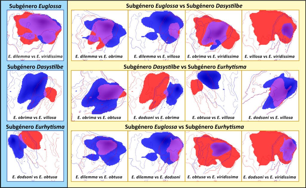
Figura 2. Comparación en el espacio ambiental de las combinaciones de pares de las especies de Euglossa analizadas. Del lado izquierdo, con fondo azul claro se encuentran las comparaciones para especies dentro del mismo subgénero. Mientras que, del lado derecho en amarillo, se muestran las comparaciones para especies de distintos subgéneros. Dentro de cada comparación, en azul rey se muestran las condiciones ambientales cubiertas por el nicho de la primera especie, en rojo las condiciones ambientales cubiertas por la segunda especie y en morado las condiciones ambientales cubiertas por ambas especies.
En cuanto a la comparación entre las especies del subgénero Euglossa y las especies de los otros 2 subgéneros, se observaron altos niveles de superposición. Resaltan las comparaciones que involucran a E. viridissima con el resto de las especies analizadas, todas con valores significativos. Euglossa viridissima tiene una distribución relativamente amplia, con reportes que sugieren posibles extensiones de rango recientes (Falcón-Brindis et al., 2018), algo similar a lo documentado para E. dilemma (Genaro et al., 2020; Skov y Wiley, 2005). La presencia y capacidad de ocupación de sitios con un amplio rango de condiciones en el caso de E. viridissima explican las similitudes significativas con las demás especies consideradas en este estudio.
Silva et al. (2014) analizaron el conservadurismo del nicho en 2 géneros de la tribu Euglossini (Eulaema y Eufriesea). Concluyeron que las especies simpátricas muestran un mayor traslape de nicho independientemente de su parentesco, a diferencia de las especies alopátricas que, aunque están más cercanamente relacionadas, presentan un menor grado de similitud de nicho. Este fenómeno no solo se observó en abejas, sino también en investigaciones con ranas de la familia Dendrobatidae (Graham et al., 2004), lagartijas del género Anolis (Losos et al., 2003) y aves del género Sylvia (Böhning-Gaese et al., 2003).
Por otro lado, existen investigaciones que respaldan la hipótesis de conservadurismo de nicho, como es el caso de ciertos grupos de plantas (Guo et al., 2013; Kolanowska, 2013; Prinzig et al., 2001), otros insectos (Peterson et al., 1999; Zhao et al., 2019), reptiles (Dowell y Hekkala, 2016; Schulte et al., 2012), anfibios (Kozak y Wiens, 2006; Muñoz-Ortiz et al., 2015), aves (Navarro-Sigüenza et al., 2020; Trujillo-Arias et al., 2018; Wang et al., 2017) y mamíferos (Peterson et al., 1999).
De acuerdo con Wiens y Graham (2005), el conservadurismo de nicho puede surgir de 4 factores clave: la selección natural, el flujo genético, la pleiotropía y la falta de variabilidad. Sin embargo, los rasgos fisiológicos (adaptaciones) que subyacen al conservadurismo de nicho están poco estudiados y pueden ser relativamente específicos de cada especie. Ellos sugieren que el estudio del conservadurismo de nicho debería centrarse en los factores que lo generan, en lugar de un debate sobre su existencia.
Los resultados obtenidos en este estudio son consistentes con investigaciones previas y refuerzan la conclusión planteada por Silva et al. (2014). En este sentido, los pares de especies hermanas en los subgéneros Dasystilbe (E. obrima + E. villosa) y Eurhytisma (E. obtusa + E. dodsoni) mostraron una menor similitud de nicho, lo cual concuerda con los estudios arriba mencionados, ya que dichas especies son actualmente alopátricas. En las comparaciones entre subgéneros. las especies alopátricas y no relacionadas mostraron baja similitud y traslape, mientras que las especies que no están cercanamente emparentadas, pero son simpátricas presentaron una mayor similitud y traslape de nicho. Un caso interesante es la similitud encontrada entre E. villosa y E. dodsoni, especies simpátricas que no están estrechamente relacionadas, en donde se observa un alto grado de similitud de nicho, aunque no fue significativo. El tamaño de la muestra puede influir en este resultado, especialmente en el caso de E. villosa, que cuenta con muy pocos registros.
Aunque se considera que la similitud de nichos encontrada en 2 de los subgéneros depende principalmente de una historia biogeográfica similar en lugar de una relación de parentesco, no se descarta que algunos factores ecológicos, como las preferencias de aroma de los machos, las tasas de competencia o las diferencias de microhábitat (Silva et al., 2014), también impacten en la dinámica temporal y espacial del nicho ecológico de las especies. Sin embargo, debido al enfoque y escala del estudio, no se puede determinar su influencia. Además, la cantidad limitada de datos utilizados, especialmente en 2 especies (E. villosa y E. obtusa) y el método empleado pudieron haber influido en los resultados obtenidos (Peterson, 2011; Warren et al., 2008).
Agradecimientos
Este proyecto fue desarrollado gracias al apoyo del programa UNAM DGAPA-PAPIIT, proyecto IN211121 y formó parte de los estudios dirigidos a la obtención del grado de Maestra en Ciencias Biológicas (Posgrado en Ciencias Biológicas, UNAM) de la primera autora, para lo cual recibió una beca de posgrado de Secihti (antes Conahcyt).
Apéndice. Capas ambientales obtenidas en diferentes bases de datos, las capas con asterisco (*) corresponden a las utilizadas en las comparaciones de superposición de pares de especies.
| Clave | Capa | Unidades | Origen |
| Bio 1* | Temperatura media anual | °C*10 | WorldClim |
| Bio 2* | Rango diurno medio (media mensual* [temp. máx.-temp. min.]) | °C*10 | WorldClim |
| Bio 3* | Isotermalidad ([BIO2 / BIO7] [100]) | °C*10 | WorldClim |
| Bio 4* | Estacionalidad de la temperatura (desv. estándar*100) | °C*10 | WorldClim |
| Bio 5* | Temperatura máxima del mes más cálido | °C*10 | WorldClim |
| Apéndice. Continúa | |||
| Clave | Capa | Unidades | Origen |
| Bio 6* | Temperatura mínima del mes más frío | °C*10 | WorldClim |
| Bio 7* | Rango anual de temperatura (Bio 5-Bio 6) | °C*10 | WorldClim |
| Bio 8* | Temperatura media del trimestre más cálido | °C*10 | WorldClim |
| Bio 9* | Temperatura media del trimestre más frío | °C*10 | WorldClim |
| Bio 10* | Precipitación anual | mm | WorldClim |
| Bio 11* | Precipitación del mes más húmedo | mm | WorldClim |
| Bio 12* | Precipitación del mes más seco | mm | WorldClim |
| Bio 13* | Estacionalidad de la precipitación (coef. var.) | mm | WorldClim |
| Bio 14 | Precipitación del trimestre más húmedo | mm | WorldClim |
| Bio 15 | Precipitación del trimestre más seco | mm | WorldClim |
| Bio 16* | Humedad específica máxima anual | kg agua/kg aire | MERRAclim |
| Bio 17* | Humedad específica máxima del mes más húmedo | kg agua/kg aire | MERRAclim |
| Bio 18* | Humedad específica máxima del mes menos húmedo | kg agua/kg aire | MERRAclim |
| Bio 19 | Estacionalidad de la humedad específica máxima (coef. var.) | kg agua/kg aire | MERRAclim |
| Bio 20 | Humedad específica máxima del trimestre más húmedo | kg agua/kg aire | MERRAclim |
| Bio 21 | Humedad específica máxima del trimestre menos húmedo | kg agua/kg aire | MERRAclim |
| Bio 22 | Humedad específica media anual | kg agua/kg aire | MERRAclim |
| Bio 23* | Humedad específica media del mes más húmedo | kg agua/kg aire | MERRAclim |
| Bio 24 | Humedad específica media del mes menos húmedo | kg agua/kg aire | MERRAclim |
| Bio 25* | Estacionalidad de la humedad específica media (coef. var.) | kg agua/kg aire | MERRAclim |
| Bio 26 | Humedad específica media del trimestre más húmedo | kg agua/kg aire | MERRAclim |
| Bio 27* | Humedad específica media del trimestre menos húmedo | kg agua/kg aire | MERRAclim |
| Bio 28 | Humedad específica mínima anual | kg agua/kg aire | MERRAclim |
| Bio 29 | Humedad específica mínima del mes más húmedo | kg agua/kg aire | MERRAclim |
| Bio 30 | Humedad específica mínima del mes menos húmedo | kg agua/kg aire | MERRAclim |
| Bio 31* | Estacionalidad de la humedad específica mínima (coef. var.) | kg agua/kg aire | MERRAclim |
| Bio 32 | Humedad específica mínima del trimestre más húmedo | kg agua/kg aire | MERRAclim |
| Bio 33 | Humedad específica mínima del trimestre menos húmedo | kg agua/kg aire | MERRAclim |
Referencias
Ascher, J. S. y Pickering, J. (2018). Discover life bee species guide and world checklist (Hymenoptera: Apoidea: Anthophila). Recuperado el 11 noviembre, 2022 de: http://www.discoverlife.org/mp/20q?guide=Apoidea_species
Böhning-Gaese, K., Schuda, M. D. y Helbig, A. J. (2003). Weak phylogenetic effects on ecological niches of Sylvia warblers. Journal of Evolutionary Biology, 16, 956–965. https://doi.org/10.1046/j.1420-9101.2003.00605.x
Bougeard, S. y Dray, S. (2018). Supervised multiblock analysis in R with the ade4 Package. Journal of Statistical Software, 86, 1–17. https://doi.org/10.18637/jss.v086.i01
Brand, P., Hinojosa-Díaz, I. A., Ayala, R., Daigle, M. Yurrita, C. L., Eltz, T. et al. (2020). The evolution of sexual signaling is linked to odorant receptor tuning in perfume-collecting orchid bees. Nature Communications, 11, 1–11. https://doi.org/10.1038/s41467-019-14162-6
Broennimann, O., Di Cola, V. y Guisan, A. (2021). ecospat: Spatial Ecology Miscellaneous Methods. R package version 3.2. https://CRAN.R–project.org/package=ecospat
Broennimann, O., Fitzpatrick, M. C., Pearman, P. B., Petitpierre, B., Pellissier, L., Yoccoz, N. G. et al. (2012). Measuring ecological niche overlap from occurrence and spatial environmental data. Global Ecology and Biogeography, 21, 481–497. https://doi.org/10.1111/j.1466-8238.2011.00698.x
Chessel, D., Dufour, A. y Thioulouse, J. (2004). The ade4 Package – I: One–Table Methods. R News, 4, 5–10.
Conabio (Comisión Nacional para el Conocimiento y Uso de la Biodiversidad). (2021). Sistema Nacional de Información sobre Biodiversidad. Registros de ejemplares. Ciudad de México, México. Recuperado el 27 febrero, 2021 de: https://www.snib.mx/
Dowell, R. y Hekkala, S. (2016). Divergent lineages and conserved niches using ecological niche modeling to examine the evolutionary patterns of the Nile monitor (Varanus niloticulus). Evolutionary Ecology, 30, 471–485. https://doi.org/10.1007/s10682-016-9818-7
Dray, S. y Dufour, A. (2007). The ade4 Package: implementing the duality diagram for ecologists. Journal of Statistical Software, 22, 1–20. https://doi.org/10.18637/jss.v022.i04
Dray, S., Dufour, A. y Chessel, D. (2007). The ade4 Package – II: Two–Table and K–Table Methods. R News, 7, 47–52.
Eliosa, H. R., Nieto, A. y Navarro, M. C. (2010). Conservadurismo filogenético del nicho ecológico un enfoque integral de la evolución. Ciencias, 98, 64–69.
Eltz, T., Fritzsch, F., Zimmermann, Y., Pech, J., Ramírez, S. R., Quezada-Euan, J. J. G. et al. (2011). Characterization of the orchid bee Euglossa viridissima (Apidae: Euglossini) and a novel cryptic sibling species, by morphological, chemical, and genetic characters. Zoological Journal of the Linnean Society, 163, 1064–1076. https://doi.org/10.1111/j.1096-3642.2011.00740.x
Engel, M. S. (2021). A key to the subgenera of the orchid bee genus Euglossa (Hymenoptera: Apidae). Entomologist’s Monthly Magazine, 157, 225–241. https://doi.org/10.31184/M00138908.1574.4093
Engel, M. S. y Rasmussen, C. (2020). Corbiculate Bees. En C. K. Starr (Ed.), Encyclopedia of Social Insects (pp. 1–9). Berlín: Springer. https://doi.org/10.1007/978-3-319-90306-4_30-1
Falcón-Brindis, A., Ayala, R., Jiménez, M. L. e Hinojosa-Díaz, I. A. (2018). A missing piece in the puzzle: the presence of Euglossa viridissima in the Baja California Peninsula (Hymenoptera, Apidae). Zookeys, 726, 15–23. https://doi.org/10.3897/zookeys.726.19876
Fick, S. E. y Hijmans, R. J. (2017). WorldClim 2: new 1 km spatial resolution climate surfaces for global land areas. International Journal of Climatology, 37, 4302–4315. https://doi.org/10.1002/joc.5086
GBIF.org (2021). Euglossa dilemma. Euglossa obrima. Euglossa dodsoni. Euglossa obtusa. Euglossa villosa. Euglossa viridissima. Recuperados el 20 julio, 2021 de: https://doi.org/10.15468/dl.xdqhq4; https://doi.org/10.15468/dl.2r57f4; https://doi.org/10.15468/dl.t6k4r6; https://doi.org/10.15468/dl.ubgt7v; https://doi.org/10.15468/dl.4xv2t2; https://doi.org/10.15468/dl.7fa7qr
Genaro, J. A., Hinojosa-Díaz, I. A. y McDowell, A. (2020). First record of the orchid bee Euglossa dilemma (Hymenoptera: Apidae) in Hispaniola, the Antilles. Insecta Mundi, 0779, 1–5.
Ghassemi-Khademi, T. (2018). New insight into the phylogeny of the orchid bees (Apidae: Euglossini). Journal of Wildlife and Biodiversity, 2, 19–35. https://doi.org/10.22120/jwb.2018.30117
Graham, C. H., Ron, S. R., Santos, J. C., Schneider, C. J. y Moritz, C. (2004). Integrating phylogenetics and environmental niche models to explore speciation mechanisms in Dendrobatid frogs. Evolution, 58, 1781–1793. https://doi.org/10.1111/j.0014-3820.2004.tb00461.x
Guo, W. Y., Lambertini, C., Li, X. Z., Meyerson, L. A. y Brix, H. (2013). Invasion of old world Phragmites australis in the new world: precipitation and temperature patterns combined with human influences redesign the invasive niche. Global Change Biology, 19, 3406–3422. https://doi.org/10.1111/gcb.12295
Hanley, J. A. y McNeil, B. J. (1982). The meaning and use of the area under a Receiver Operating Characteristic Curve (ROC). Diagnostic Radiology, 143, 29–36. https://doi.org/10.1148/radiology.143.1.7063747
Henske, J., Saleh, N. W., Chouvenc, T., Ramírez, S. R. y Eltz, T. (2023). Function of environment-derived male perfumes in orchid bees. Current Biology, 33, 2075–2080. https://doi.org/10.1016/j.cub.2023.03.060
Hijmans, R. J., Phillips, S., Leathwick, J. y Elith, J. (2020). Dismo: species distribution modeling. R package version 1.3-3. https://CRAN.R-project.org/package=dismo
Hinojosa-Díaz, I. A. y Engel, M. S. (2011). Euglossa williamsi, a new species of orchid bee from the Amazon Basin of Ecuador and Peru, with notes on its taxonomic association and biogeography (Hymenoptera, Apidae). Zookeys, 159, 49–63. https://doi.org/10.3897/zookeys.159.2239
Hinojosa-Díaz I. A., Melo G. y Engel, M. (2011). Euglossa obrima, a new species of orchid bee from Mesoamerica, with notes on the subgenus Dasystilbe Dressler (Hymenoptera, Apidae). Zookeys, 97, 11–29. https://doi.org/10.3897/zookeys.97.1106
Kass, J. M., Vilela, B., Aiello-Lammens, M. E., Muscarella, R., Merow, C. y Anderson, R. P. (2018). Wallace: a flexible platform for reproducible modeling of species niches and distributions built for community expansion. Methods in Ecology and Evolution, 9, 1151–1156. https://doi.org/10.1111/2041-210X.12945
Kass, J. M., Muscarella, R., Galante, P. J., Bohl, C. L., Pinilla-Buitrago, G. E., Boria, R. A. et al. (2021). ENMeval 2.0: redesigned for customizable and reproducible modeling of species’ niches and distributions. Methods in Ecology and Evolution, 12, 1602–1608. https://doi.org/10.1111/2041-210X.13628
Kolanowska, M. (2013). Niche conservatism and the future potential range of Epipactis helleborine (Orchidaceae). Plos One, 8, 1–8. https://doi.org/10.1371/journal.pone.0077352
Kozak, K. H. y Wiens, J. J. (2006). Does niche conservatism promote speciation? A case study in North American salamanders. Evolution, 60, 2604–2621. https://doi.org/
10.1111/j.0014-3820.2006.tb01893.x
Losos, J. B., Jackman, T. R., Larson, A., de Queiroz, K. y Rodríguez-Schettino, L. (1998). Contingency and determinism in replicated adaptive radiations of island lizards. Science, 279, 2115–2118. http://www.jstor.org/stable/2896277
Morrone, J. J., Escalante, T., Rodríguez-Tapia, G., Carmona, A., Arana, M. y Mercado-Gómez, J. D. (2022). Biogeographic regionalization of the neotropical region: new map and shapefile. Anais da Academia Brasileira de Ciencias, 94, e20211167. https://doi.org/10.1590/0001-3765202220211167
Moure, J. S. y Melo, G. A. R. (2023). Euglossini Latreille, 1802. En Moure, J. S., Urban, D. & Melo, G. A. R. (Orgs). Catalogue of Bees (Hymenoptera, Apoidea) in the Neotropical Region – online version. Disponible en: https://www.moure.cria.org.br/catalogue
Muñoz-Ortiz, A., Velásquez-Álvarez, Á. A., Guarnizo, C. E. y Crawford, A. J. (2015). Of peaks and valleys: testing the roles of orogeny and habitat heterogeneity in driving allopatry in mid-elevation frogs (Aromobatidae: Rheobates) of the northern Andes. Journal of Biogeography, 42, 193–205. https://doi.org/10.1111/JBI.12409
Navarro-Sigüenza, A. G., Almazán-Núñez, R. C., Sánchez-Ramos, L. E., Rebón-Gallardo, M. F. y Arbeláez-Cortés, E. (2020). Relict humid tropical forest in Mexico promotes differentiation in barred woodcreepers Dendrocolaptes (Aves: Furnariidae). Zootaxa, 4780, 307–323. https://doi.org/10.11646/zootaxa.4780.2.5
Pearson, R. G., Raxworthy, C. J., Nakamura, M. y Peterson, A. T. (2007). Predicting species distributions from small numbers of occurrence records: a test case using cryptic geckos in Madagascar. Journal of Biogeography, 34, 102–117. https://doi.org/10.1111/j.1365-2699.2006.01594.x
Peterson, A. T. (2011). Ecological niche conservatism: a time-structured review evidence. Journal of Biogeography, 38, 817–827. https://doi.org/10.1111/j.1365-2699.2010.02456.x
Peterson, A. T., Soberón, J. y Sánchez-Cordero, V. (1999). Conservatism of ecological niches in evolutionary time. Science, 285, 1265–1267. https://doi.org/10.1126/science.285.5431.1265
Phillips, S. J., Anderson, R. P. y Schapire, R. E. (2006). Maximum entropy modeling of species geographic distributions. Ecological Modelling, 190, 231–259. https://doi.org/10.1016/j.ecolmodel.2005.03.026
Pokorny, T., Loose, D., Dyker, G., Quezada-Euán, J. J. G. y Eltz, T. (2015). Dispersal ability of male orchid bees and direct evidence for long-range flights. Apidologie, 46, 224–237. https://doi.org/10.1007/s13592-014-0317-y
Prinzig, A., Durka, W., Klotz, S. y Brandl, F. (2001). The niche of higher plants: evidence for phylogenetic conservatism. Proceedings: Biological Sciences, 268, 2383–2389. https://doi.org/10.1098/rspb.2001.1801
Pyron, R. A., Costa, G. C., Patten, M. A. y Burbrink, F. T. (2015), Phylogenetic niche conservatism and the evolutionary
basis of ecological speciation. Biological Reviews, 90, 1248–1262. https://doi.org/10.1111/brv.12154
R Core Team (2020). R: a language and environment for statistical computing. R Foundation for Statistical Computing, Vienna, Austria. https://www.R–project.org/.
Ramírez, S. R., Roubik, D. W., Skov, C. y Pierce, N. E. (2010). Phylogeny, diversification patterns and historical biogeography of euglossine orchid bees (Hymenoptera: Apidae). Biological Journal of the Linnean Society, 100, 552–572. https://doi.org/10.1111/j.1095-8312.2010.01440.x
Roubik, D. W. y Hanson, P. (2004). Orchid bees: biology and field guide. Heredia, Costa Rica: INBio.
Schoener, T. W. (1968). The Anolis lizards of Bimini: resource partitioning in a complex fauna. Ecology, 49, 704–726. https://doi.org/10.2307/1935534
Schulte, U., Hochkirch, A., Lötters, S., Rödder, D., Schweiger, S., Weimann, T. et al. (2012). Cryptic niche conservatism among evolutionary lineages of an invasive lizard. Global Ecology and Biogeography, 21, 198–211. https://doi.org/10.1111/j.1466-8238.2011.00665.x
Shcheglovitova, M. y Anderson, R. P. (2013). Estimating optimal complexity for ecological niche models: a jackknife approach for species with small sample sizes. Ecological Modelling, 269, 9–17. https://doi.org/10.1016/j.ecolmodel.2013.08.011
Silva, D. P., Vilela, B., De Marco, P. y Nemésio, A. (2014). Using ecological niche models and niche analyses to understand speciation patterns: the case of sister neotropical orchid bees. Plos One, 9, e113246. https://doi.org/10.1371/journal.pone.0113246
Skov, C. y Wiley, J. (2005). Establishment of the neotropical orchid bee Euglossa viridissima (Hymenoptera: Apidae) in Florida. Florida Entomologist, 88, 225–227. https://doi.org/10.1653/0015-4040(2005)088[0225:EOTNOB]2.0.CO;2
Thioulouse, J., Dray, S., Dufour, A., Siberchicot, A., Jombart, T. y Pavoine, S. (2018). Multivariate Analysis of Ecological Data with ade4. Nueva York: Springer. https://doi.org/10.1007/978-1-4939-8850-1
Trujillo-Arias, N., Calderón, L., Santos, F. R., Miyaki, C. Y., Aleixo, A., Witt, C. C. et al. (2018). Forest corridors between the central Andes and the southern Atlantic Forest enabled dispersal and peripatric diversification without niche divergence in a passerine. Molecular Phylogenetics and Evolution, 128, 221–232. https://doi.org/10.1016/j.ympev.2018.08.005
Vega, G. C., Pertierra, L. R. y Olalla-Tárraga, M. A. (2018). MERRAclim, a high-resolution global dataset of remotely sensed bioclimatic variables for ecological modelling. Scientific Data, 4, 170078. https://doi.org/10.1038/sdata.2017.78
Wang, P., Liu, Y., Liu, Y., Chang, Y., Wang, N. y Zhang, Z. (2017). The role of niche divergence and geographic arrangement in the speciation of Eared Pheasants (Crossoptilon, Hodgson 1938). Molecular Phylogenetics and Evolution, 113, 1–8. https://doi.org/10.1016/j.ympev.2017.05.003
Warren, D. J., Glor, R. E. y Turelli, M. (2008). Environmental niche equivalency versus conservatism: quantitative approaches to niche evolution. Evolution, 62, 2868–2883. https://doi.org/10.1111/j.1558-5646.2008.00482.x
Wiens, J. J. y Donoghue, M. J. (2004). Historical biogeography, ecology and species richness. Trends in Ecology and Evolution, 19, 639–644. https:/doi.org/10.1016/j.tree.
2004.09.011
Wiens, J. J. y Graham, C. H. (2005). Niche conservatism: integrating evolution, ecology, and conservation biology. Annual Review of Ecology, Evolution, and Systematics, 36, 519–539. https://doi.org/10.1146/annurev.ecolsys.36.102803.095431
Zhao, Q., Zhang, H. y Wei, J. (2019). Climatic niche comparison across a cryptic species complex. PeerJ, 2019, 1–18. https://doi.org/10.7717/peerj.7042

Updated species list, distribution and modeling of alpine mosses in central Mexico
Lista actualizada de especies, distribución y modelaje de musgos alpinos del centro de México
Claudio Delgadillo-Moya a, *, Ana Paola Peña-Retes a, Carlos Cerrejónb
a Universidad Nacional Autónoma de México, Instituto de Biología, Departamento de Botánica, Apartado postal 70-233, 04510 Ciudad de México, Mexico
b Independent researcher
*Corresponding author: moya@ib.unam.mx (C. Delgadillo-Moya)
Received: 18 February 2025; accepted: 26 November 2025
Abstract
The Neovolcanic Belt of central Mexico is a phytogeographically significant region that influenced moss distribution patterns in the Americas. Its alpine moss flora was updated in 1971, but species range information remains fragmentary. This study updates the list and distribution of alpine mosses in the Neovolcanic Belt, and improves our understanding of these ranges by developing species distribution models (SDMs) for 4 mosses. Hypothetically, mosses reached alpine tops by migration. At lower elevations, interchange by corridors across the Belt connected ecologically similar areas and brought other species to alpine elevations. This can be tested using SDMs. SDMs provided high to relatively high prediction accuracy for all modeled species (mAUC = 0.88 ± 0.06; mCBI = 0.72 ± 0.09), and confirmed the corridor hypothesis. Overall, elevation emerged as the most important distribution predictor of target species, showing a positive sigmoidal relationship with environmental suitability. Our models effectively captured an integrated climatic signal via elevation, due to its strong negative correlation with several temperature- and precipitation-related predictors. Out of 120 alpine mosses, some are widespread in central Mexico while others are mainly distributed in eastern or western mountains. Additional fieldwork and ecological research are essential to further clarify their distribution.
Keywords: Bryophyta; Digital mapping; Machine learning; Maxent; Mexican highlands; Predictive modeling; Species distribution models
Resumen
El Eje Neovolcánico ha influido en los patrones de distribución continental de musgos. Desde 1971, no se revisaba el número y la distribución de especies alpinas. Este trabajo actualiza el listado para el Eje Neovolcánico y explica la distribución mediante modelos de distribución de especies (SDM) para 4 casos seleccionados. En teoría, los musgos se distribuyeron por migración entre zonas alpinas. El intercambio mediante corredores entre sitios ecológicamente similares de elevaciones más bajas permitió el ingreso de otras especies. Los SDM ofrecieron predicciones precisas, de alta a relativamente alta, para todas las especies modeladas (mAUC = 0.88 ± 0.06; mCBI = 0.72 ± 0.09) y confirmaron la hipótesis de los corredores. En general, la elevación fue el predictor más importante de distribución de especies, mostrando una relación sigmoidal positiva con la idoneidad ambiental. Tales modelos capturaron de manera efectiva la señal climática integrada a través de la elevación, por su fuerte correlación negativa con varios predictores relacionados con temperatura y precipitación. De 120 taxones de musgos alpinos, unos tienen distribución generalizada, otros se distribuyen principalmente en las montañas del este o del oeste. Trabajo de campo adicional explicaría mejor la distribución.
Palabras clave: Bryophyta; Mapeo digital; Aprendizaje automático; Maxent; Elevaciones mexicanas; Modelaje predictivo; Modelos de distribución
Introduction
Except for Bartram (1945, 1949) there is no major reference to alpine mosses (i.e., from above timberline) in the early bryological literature for Mexico. Floristic information frequently refers to highland moss collections with incidental direct or indirect reference to alpine species (e.g., Cardot, 1909a, b, c, 1910a, b, c, d, 1911; Hooker, 1818, 1820; Thériot, 1921, 1931, 1933). In the early 1970, results of fieldwork produced a preliminary evaluation and a list of 84 taxa in alpine habitats of central and northern Mexico (Delgadillo, 1971). Study of additional collections brought the number of mosses to 111 taxa (Delgadillo, 1984, 1987) representing 5 floristic elements (Northern, Meso-American, Southern, Wide-ranging, Endemic) according to their world ranges. These ranges were explained on the basis of hypotheses supported by ecological, geological, and geographical considerations as part of a project on the phytogeographical role of the Neovolcanic Belt of central Mexico (Delgadillo, 1985, 1987, 1988). The species shared among mountain tops indicate that these areas act as stepping-stones for moss migration and that the Mexican highlands have participated in significant floristic exchange in the Americas. Furthermore, it seems that the Neovolcanic Belt mountains also served as an incomplete barrier to moss interchange due to their geographical position and uneven elevation, especially between northern and southern areas on either side of the range. According to Delgadillo (1988, 1992, 1998, 2009) moss distribution through 7 lowland topographic discontinuities suggest that they are pathways (corridors) for migration across the Belt. Corridors in the Neovolcanic Belt occur at elevations of approximately 2,000 m in the northern portion, descending to around 1,500 m in southern areas, with some reaching up to 2,800 m (Delgadillo, 1988, 1998). These corridors contain mixed contingents of high- and lowland moss species.
The high number of species shared among alpine areas seems to support the hypothesis on the presumed interchange along the mountains of the Neovolcanic Belt. In theory, the colonizing species could spread from 1 or several points of arrival and extend their ranges toward other alpine or subalpine habitats. Modern populations are descendants already adapted to high elevations that occupy new microhabitats in the corridors.
The floristic patterns of the moss flora in the highlands are poorly represented because of the low number of samples and data collected from the alpine areas or across elevation gradients. Species distribution models (SDMs) provide useful tools for filling existing knowledge gaps on species ranges in underexplored areas by quantifying the statistical relationships between species observations and environmental conditions from known locations and spatializing these relationships across the landscape (Guillera-Arroita et al., 2015; Mateo et al., 2011). SDMs can thus offer explanations as to how current species distribution patterns became established.
This paper aims to provide a comprehensive updated list of alpine mosses and their known distribution in the Neovolcanic Belt of central Mexico, and improve our understanding of these ranges by predicting the distribution of 4 moss species selected as case studies using SDMs. We hypothesize that in addition to migration among mountain tops, moss interchange across the Neovolcanic Belt occurs via corridors connecting ecologically similar areas, as suggested by the distribution of species along the Belt (Delgadillo, 1988, 1998, 2009). SDMs were built using Maxent machine learning, which is based on the principle of maximum entropy, and known to provide accurate predictions of species distribution using presence-only data (Phillips et al., 2006; Phillips & Dudík, 2008).
Materials and methods
A revised list of alpine mosses (Table 1) in central Mexico was obtained from published records, especially the previous listing (Delgadillo, 1987), and from current herbarium holdings at MEXU; updates came from fieldwork or unreported specimens. The TROPICOS database (https://www.tropicos.org/home), the Bryophyte Nomenclator (https://www.bryonames.org), and the International Plant Names Index (https://www.ipni.org/?) were consulted for floristic and taxonomic information.
Known distribution ranges of alpine mosses
Herbarium information and data from a revised digital LATMOSS (Delgadillo et al., 1995) were then compiled to obtain the altitudinal range for each alpine moss cited in Table 1. Several species such as Leptodontium viticulosoides, Orthotrichum pycnophyllum, and Zygodon ehrenbergii frequently grow as epiphytes on phorophytes living above timberline in protected habitats; epiphytic mosses may still be labelled as alpine. Also, mosses growing in sites close to timberline, but slightly below its average altitude, may still be considered as alpine. This situation applies to various specimens whose stated altitudinal range does not reach 4,000 m. Timberline elevation varies in central Mexico; in such volcanoes as Iztaccíhuatl and Popocatépetl the mean elevation value is 4,020 m and 3,911 m, respectively, as shown by Beaman (1962). Specimens of Astomiopsis amblyocalyx and A. exserta were reported as alpine (Bartram, 1949), but since no other collections at MEXU are truly alpine, they are only listed for 2 mountains in this report. Old specimens and literature records without habitat or elevation, were not included in the original list for the alpine flora.
Table 1 distinguishes 5 groups of species. Each group includes species common to 1 or more alpine areas as represented by specimens collected there. The groups provide preliminary information on the potential distribution of the alpine moss flora in the mountains of central Mexico. Most species are distributed elsewhere, and their known altitudinal range may be an indication of their local vertical potential. Information on life-form describing the ecological response of mosses is also cited as this may offer insights on their adaptation to life in the highland environment.
Table 1
Revised list of alpine taxa and their distribution in the Neovolcanic Belt of central Mexico, known altitudinal range (Alt-rge), local distribution groups, and life-form. Abbrev.: N-COL = Nevado de Colima, IZTA = Iztaccíhuatl, POPO = Popocatépetl, TOL = Nevado de Toluca, MAL = La Malinche, P-ORIZ = Pico de Orizaba, C-PER = Cofre de Perote. C = Inland-mountain distribution, G = generalized, C-E = inland- eastern mountains, W-C = western-inland mountains, E = eastern mountains.
| Taxa | N-COL | IZTA | POPO | TOL | MAL | P-ORIZ | C-PER | Alt-rge (m asl) | Group | Life-form |
| Aligrimmia peruviana R.S. Williams | 1 | 4,150 | C | short tufts | ||||||
| Aloinella catenula Cardot | 1 | 1 | 1 | 1 | 1 | 1 | 1 | 2,500-4,020 | G | tufts |
| Amphidium tortuosum (Hornsch.) Cufod. | 1 | 1 | 1 | 1 | 1 | 2,000-4,550 | G | tufts or cushions | ||
| Anacolia laevisphaera (Taylor) Flowers | 1 | 1 | 1 | 1,800-4,400 | C-E | loose tufts | ||||
| Andreaea rupestris Hedw. | 1 | 1 | 1 | 1 | 1 | 1 | 1 | 2,950-4,420 | G | tufts or mats |
| Anoectangium aestivum (Hedw.) Spruce | 1 | 1 | 1 | 96-4,400 | C | tufts | ||||
| Anomobryum julaceum (Schrad. ex G. Gaertn., B. Mey. & Scherb.) Schimp. | 1 | 1 | 1 | 1 | 200-4,570 | W-C | tufts | |||
| Anomobryum prostratum (Müll. Hal.) Besch. | 1 | 1 | 1 | 1 | 1 | 1 | 1 | 1,700-4,700 | G | tufts |
| Table 1. Continued | ||||||||||
| Taxa | N-COL | IZTA | POPO | TOL | MAL | P-ORIZ | C-PER | Alt-rge (m asl) | Group | Life-form |
| Aongstroemia julacea (Hook.) Mitt. | 1 | 1 | 1 | 1 | 1 | 2,900-4,500 | G | loose tufts | ||
| Aongstroemia orientalis Mitt. | 1 | 1 | 1 | 1 | 1 | 1 | 1 | 1,700-4,350 | G | loose tufts |
| Astomiopsis amblyocalyx Müll. Hal. | 1 | 1 | 3,370-3,600 | C | tufts | |||||
| Astomiopsis exserta (E. B. Bartram) Snider | 1 | 3,370-3,600 | C | tufts | ||||||
| Bartramia brevifolia Brid. | 1 | 1 | 1 | 1 | 1 | 1 | 1,300-4,000 | G | loose or dense tufts | |
| Bartramia ithyphylla Brid. | 1 | 1 | 1 | 3,000-4,180 | C-E | loose or dense tufts | ||||
| Bartramia microstoma Mitt. | 1 | 1 | 1 | 1 | 1 | 1 | 2,636-4,350 | G | loose or dense tufts | |
| Bartramia potosica Mont. | 1 | 1 | 1 | 1 | 1 | 1 | 1 | 2,636-4,350 | G | loose or dense tufts |
| Brachymenium systylium (Müll. Hal.) A. Jaeger | 1 | 1 | 1 | 1,060-3,375 | G | dense tufts | ||||
| Brachythecium frigidum (Müll. Hal.) Besch. | 1 | 1 | 1 | 1 | 1 | 2,652-4,175 | C-E | mats or tufts | ||
| Brachythecium occidentale (Hampe) A. Jaeger | 1 | 1 | 1 | 1 | 2,700-4,230 | C-E | mats or tufts | |||
| Brachythecium plumosum (Hedw.) Schimp. | 1 | 1 | 1 | 1,450-4,200 | C | mats or tufts | ||||
| Brachythecium ruderale (Brid.) W. R. Buck | 1 | 1 | 1 | 1 | 1 | 1 | 1 | 1,150-4,230 | G | mats or tufts |
| Brachythecium salebrosum (Hoffm. ex F. Weber & D. Mohr) Schimp. | 1 | 1 | 2,350-3,962 | C-E | mats or tufts | |||||
| Braunia imberbis (Sm.) N. Dalton & D.G. Long | 1 | 1 | 1 | 1 | 1 | 2,300-3,950 | G | mats or tufts | ||
| Breutelia subarcuata (Müll. Hal.) Schimp. | 1 | 1 | 1 | 1,800-alpine | W-C | dense tufts | ||||
| Bryoerythrophyllum bolivianum (Müll. Hal.) R. H. Zander | 1 | 3,580-3,900 | E | loose or dense tufts | ||||||
| Bryoerythrophyllum calcareum (Thér.) R. H. Zander | 1 | 2,600-3,750 | C | loose or dense tufts | ||||||
| Bryoerythrophyllum campylocarpum (Müll. Hal.) H. A. Crum | 1 | 1 | 2,030-4,100 | C | loose or dense tufts | |||||
| Bryoerythrophyllum ferruginascens (Stirt.) Giac. | 1 | 1 | 1 | 2,500-4,000 | C | loose or dense tufts | ||||
| Bryoerythrophyllum jamesonii (Taylor) H. A. Crum | 1 | 1 | 1,400-4,300 | C | loose or dense tufts | |||||
| Bryoerythrophyllum recurvirostrum (Hedw.) Chen var. aeneum (Müll. Hal.) R. H. Zander | 1 | 1 | 1,700-3,910 | C-E | loose or dense tufts | |||||
| Bryoerythrophyllum recurvirostrum (Hedw.) Chen var. recurvirostrum | 1 | 1 | 1 | 1 | 1,070-3,970 | G | loose or dense tufts | |||
| Bryomanginia saint-pierrei Thér. | 1 | 1 | 3,600-4,350 | C | tufts | |||||
| Bryoxiphium norvegicum (Brid.) Mitt. var. mexicanum (Besch.) Sharp | 1 | 1 | 1 | 2,600-4,145 | C-E | loose tufts | ||||
| Bryum argenteum Hedw. | 1 | 1 | 1 | 1 | 1 | 1 | 1 | 700-4,100 | G | loose or dense tufts |
| Bryum billardieri Schwägr. | 1 | 1 | 1 | 1 | 1 | 1 | 650-4,120 | G | loose or dense tufts | |
| Bryum capillare Hedw. | 1 | 1 | 1 | 1 | 1 | 1 | 600-4,400 | G | loose or dense tufts | |
| Bryum cellulare Hook. ex Schwägr. | 1 | 2,000 | C | loose or dense tufts | ||||||
| Bryum pallescens Schleich. ex Schwägr. | 1 | 1 | 1 | 2,286-4,000 | W-C | loose or dense tufts | ||||
| Bryum pseudotriquetrum (Hedw.) Gaertn., Meyer & Scherb. | 1 | 1 | 1,859-4,000 | C | loose or dense tufts | |||||
| Campylopus albidovirens Herz. | 1 | 2,414-4,050 | C | dense tufts | ||||||
| Campylopus flexuosus (Hedw.) Brid. | 1 | 1,000-4,050 | C | dense tufts | ||||||
| Campylopus fragilis (Brid.) Bruch & Schimp. | 1 | 1 | 1,350-4,050 | C | dense tufts | |||||
| Campylopus nivalis (Brid.) Brid. | 1 | 1 | 1 | 1 | 1,420-4,050 | W-C | dense tufts | |||
| Campylopus tallulensis Sull. & Lesq. | 1 | 1 | 1 | 1 | 1,300-4,000 | C-E | dense tufts | |||
| Ceratodon purpureus (Hedw.) Brid. | 1 | 1 | 1 | 1 | 1,900-4,050 | C-E | loose or dense tufts | |||
| Ceratodon stenocarpus B.S.G. | 1 | 1 | 1 | 1 | 1 | 1 | 1 | 1,860-4,145 | G | loose or dense tufts |
| Coscinodon cribrosus (Hedw.) Spruce | 1 | 3,500-3,885 | C | dense cushions | ||||||
| Cratoneuron filicinum (Hedw.) Spruce | 1 | 1 | 2,440-3,900 | C | tufts or mats | |||||
| Dicranoweisia cirrata (Hedw.) Lindb. ex Milde | 1 | 2,450-4,050 | C | dense tufts | ||||||
| Dicranum frigidum Müll. Hal. | 1 | 2,134-4,200 | C | dense tufts | ||||||
| Dicranum rhabdocarpum Sull. | 1 | 1,700-3,900 | C | dense tufts | ||||||
| Didymodon australasiae (Hook. & Grev.) R. H. Zander | 1 | 1 | 1 | 40-4,020 | C-E | tufts or cushions | ||||
| Didymodon rigidulus Hedw. var. gracilis (Schleich. ex Hook. & Grev.) R. H. Zander | 1 | 1 | 1 | 1 | 1 | 1 | 1 | 1,220-4,200 | G | tufts or cushions |
| Didymodon rigidulus Hedw. var. icmadophilus (Schimp. ex Müll. Hal.) R. H. Zander | 1 | 1 | 1 | 550-alpine | G | tufts or cushions | ||||
| Distichium capillaceum (Hedw.) Bruch & Schimp. | 1 | 3,050-4,100 | C | dense tufts | ||||||
| Ditrichum gracile (Mitt.) Kuntze | 1 | 1 | 1 | 1 | 1 | 2,100-4,000 | C-E | dense tufts | ||
| Encalypta ciliata Hedw. | 1 | 1 | 1 | 1 | 1 | 1 | 1 | 2,580-4,300 | G | tufts |
| Fissidens crispus Mont. | 1 | 1 | 1,372-3,460 | C | tufts | |||||
| Funaria hygrometrica Hedw. | 1 | 1 | 1 | 850-4,000 | C | tufts | ||||
| Funaria orizabensis Müll. Hal. | 1 | 1,435-3,910 | E | tufts | ||||||
| Grimmia austrofunalis Müll. Hal. | 1 | 1 | 2,530-3,900 | C-E | dense tufts or cushions | |||||
| Grimmia donniana Sm. | 1 | 1 | 1 | 1 | 3,900-4,267 | C-E | dense tufts or cushions | |||
| Grimmia elongata Kaulf. | 1 | 1 | 1 | 1 | 1 | 1 | 1 | 3,700-4,520 | G | dense tufts or cushions |
| Grimmia fuscolutea Hook. | 1 | 1 | 1 | 1 | 1 | 1 | 1 | 2,432-4,200 | G | dense tufts or cushions |
| Grimmia longirostris Hook. | 1 | 1 | 1 | 1 | 1 | 1 | 1,220-4,350 | G | dense tufts or cushions | |
| Grimmia mexicana Greven | 1 | 1 | 1 | 1 | 1 | 1 | 1 | 3,500-4,300 | G | dense tufts or cushions |
| Grimmia montana Bruch & Schimp. | 1 | 1 | 1 | 1 | 1 | 1 | 1,524-4,633 | C-E | dense tufts or cushions | |
| Grimmia ovalis (Hedw.) Lindb. | 1 | 1 | 2,020-3,070 | E | dense tufts or cushions | |||||
| Grimmia torquata Drumm. | 1 | 1 | 1 | 3,750-4,267 | C-E | dense tufts or cushions | ||||
| Grimmia trichophylla Grev. | 1 | 1 | 1 | 1 | 1 | 1 | 610-4,200 | G | dense tufts or cushions | |
| Hennediella longirostris (Hampe ex Müll. Hal.) R. H. Zander | 1 | 1 | Alpine | C-E | tufts | |||||
| Hennediella polyseta (Müll. Hal.) R. H. Zander | 1 | 1 | 1 | 3,650-4,100 | C-E | tufts | ||||
| Hymenolomopsis tolucensis Thér. | 1 | 1 | 1 | 3,500-4,300 | G | tufts | ||||
| Hypnum cupressiforme Hedw. var. cupressiforme | 1 | 2,700-3,600 | C | mats | ||||||
| Hypnum cupressiforme Hedw. var. lacunosum Brid. | 1 | 1 | 1 | 1 | 2,580-4,150 | C-E | mats | |||
| Hypnum revolutum (Mitt.) Lindb. | 1 | 1 | 1 | 1 | 1 | 2,500-4,350 | C-E | mats | ||
| Leptodictyum riparium (Hedw.) Warnst | 1 | 1 | 914-3,310- alpine | W-C | mats | |||||
| Leptodontium flexifolium (Dicks. ex With.) Hampe | 1 | 1 | 1 | 1 | 1 | 1 | 1 | 1,237-4,350 | G | loose tufts |
| Leptodontium pungens (Mitt.) Kindb. | 1 | 1 | 1 | 1 | 1 | 1 | 2,375-4,380 | C-E | loose tufts | |
| Leptodontium viticulosoides (P. Beauv.) Wijk & Marg. var. viticulosoides | 1 | 1 | 1 | 1 | 1 | 1,100-4,000 | G | loose tufts | ||
| Leptodontium viticulosoides var. sulphureum (Müll. Hal.) R. H. Zander | 1 | 1 | 1 | 1 | 1,372-4,000 | C-E | loose tufts | |||
| Leptopterigynandrum tenuicaule (R.S. Williams) S. He | 1 | 1 | 1,200-4,400 | C-E | mats | |||||
| Lepyrodon tomentosus (Hook.) Mitt. | 1 | 300-4,280 | E | cushion or mats | ||||||
| Mielichhoferia argentifolia Mitt. | 1 | 1 | 1 | 3,840-4,050 | C-E | tufts | ||||
| Mironia ehrenbergiana (Müll. Hal.) R. H. Zander | 1 | 1 | 1 | 1 | 1 | 1 | 1 | 3,880-4,200 | G | tufts |
| Mironia stenotheca (Thér.) R.H. Zander | 1 | 1 | 1 | 1 | 1 | 2,870-3,962 | G | tufts | ||
| Neosharpiella aztecorum H. Rob. & Delgad. | 1 | 1 | 1 | 1 | 1 | 1 | 3,370-4,200 | C-E | tufts | |
| Notoligotrichum mexicanum (G. Smith) G. Smith | 1 | 1 | 1 | 1 | 4,350 | C | tufts | |||
| Oreoweisia erosa (Hampe ex Müll. Hal.) Kindb. | 1 | 1 | 1 | 2,140-3,700-alpine | C | tufts | ||||
| Orthodontium gracile Schwägr. ex B.S.G. | 1 | 1 | 2,600-3,970 | W-C | tufts | |||||
| Orthotrichum pycnophyllum Schimp. ex Müll. Hal. | 1 | 1 | 1 | 1,340-3,950 | C-E | tufts | ||||
| Paraleucobryum enerve (Thed. ex Hartm.) Loeske | 1 | 1 | 1 | 1 | 2,682-4,350 | C-E | dense tufts | |||
| Philonotis corticata H. A. Crum & Griff. | 1 | 1 | 1 | 1 | 1 | 1 | 1 | 3,800-4,200 | G | tufts |
| Pleuridium mexicanum Cardot | 1 | 1 | 1 | 1,859-4,050 | C | tufts | ||||
| Pogonatum jamesonii (Taylor) B.H. Allen | 1 | 1 | 1 | 1 | 1 | 1 | 1,750-4,000 | G | tufts | |
| Pohlia cruda (Hedw.) Lindb. | 1 | 1 | 1 | 1 | 1 | 1 | 1 | 3,300-4,200 | G | tufts |
| Pohlia elongata Hedw. | 1 | 1 | 1 | 1 | 1 | 1 | 1 | 1,524-4,180 | G | tufts |
| Pohlia oerstediana (Müll. Hal.) A.J. Shaw | 1 | 1 | 1 | 1 | 1 | 2,520-4,180 | G | tufts | ||
| Polytrichastrum alpinum (Hedw.) G. Smith | 1 | 1 | 1 | 1 | 1 | 1 | 3,880-4,300 | G | tufts | |
| Polytrichastrum tenellum (Müll. Hal.) G. Smith | 1 | 1 | 1 | 1 | 1 | 2,530-3,970 | G | tufts | ||
| Polytrichum juniperinum Hedw. | 1 | 1 | 1 | 1 | 1,000-4,350 | C-E | tufts | |||
| Racomitrium crispipilum (Taylor) Spruce | 1 | 1 | 1 | 1 | 1 | 2,470-4,100 | C-E | mats or tufts | ||
| Racomitrium subsecundum (Hook. & Grev. ex Harv.) Mitt. | 1 | 1 | 1 | 1 | 1 | 1 | 2,570-4,000 | G | mats or tufts | |
| Rhabdoweisia crispata (Dicks. ex With.) Lindb. | 1 | 1 | 2,900-4,020 | C | tufts | |||||
| Rhabdoweisia fugax (Hedw.) Bruch & Schimp. | 1 | 1 | 1 | 2,410-4,000 | C | tufts | ||||
| Rhytidium rugosum (Hedw.) Kindb. | 1 | 2,000-3,658 | E | tufts | ||||||
| Sagenotortula quitoensis (Taylor in Hook.) R. H. Zander | 1 | 1 | 2,240-alpine | C-E | tufts | |||||
| Sanionia uncinata (Hedw.) Loeske | 1 | 1 | 1 | 1 | 3,036-4,415 | C | mats or tufts | |||
| Saitobryum lorentzii (Müll. Hal.) Ochyra | 1 | 1 | 3,300-3,700 | C | tufts | |||||
| Schizymenium campylocarpum (Arn. & Hook.) A.J. Shaw | 1 | 1 | 1 | 1 | 1 | 1 | 2,896-4,300 | G | tufts | |
| Schizymenium schiedeanum (Müll. Hal.) A.J. Shaw | 1 | 1 | 1 | 1 | 1 | 1 | 2,760-4,100 | G | tufts | |
| Schizymenium serratum (Cardot & Herzog) A.J. Shaw | 1 | 1 | 2,600-4,000 | C-E | tufts | |||||
| Syntrichia andicola (Mont.) Ochyra | 1 | 1 | 1 | 1 | 1 | 1 | 3,700-4,430 | C-E | tufts | |
| Syntrichia obtusissima (Müll. Hal.) R. H. Zander | 1 | 200-4,300 | E | tufts | ||||||
| Syntrichia ruralis (Hedw.) Web. & Mohr | 1 | 1 | 1 | 1 | 600-4,200 | C-E | tufts | |||
| Tayloria splachnoides (Schwägr.) Hook. | 1 | 1 | 1 | 1 | 3,300-3,962 | C-E | tufts | |||
| Tristichium mirabile (Müll. Hal.) Herz. | 1 | 1 | 3,950-4,350 | C | tufts | |||||
| Zygodon ehrenbergii Müll. Hal. | 1 | 1 | 1 | 1 | 2,500-4,000 | G | tufts | |||
| Zygodon pichinchensis (Taylor) Mitt. | 1 | 1 | 1 | 1 | 1 | 1 | 3,870-4,300 | G | tufts | |
| Zygodon viridissimus (Dicks.) Brid. | 1 | 1 | 2,765-3,950 | C-E | tufts | |||||
| Total number of taxa = 120 | 48 | 86 | 72 | 85 | 44 | 62 | 65 |
Species distribution modeling of case study mosses
Herbarium and literature sources are sometimes insufficient to obtain reliable data for analysis. Various species, including Grimmia pulla, Orthotrichum pycnophyllum, and Zygodon ehrenbergii were evaluated for their distribution as corridor or alpine species. Specimens of these 3 taxa were few in number, rarely alpine and thus not entirely useful to test our hypothesis; 4 other species were selected because their habitat and elevation were well-known from various alpine localities and substrates in the Neovolcanic Belt. MEXU holds sufficient number of georeferenced specimens of Brachythecium occidentale and B. plumosum, 2 of the few pleurcarpous mosses that grow mainly on soil or rocks. Grimmia longirostris and G. trichophylla are broadly represented in our records, they are acrocarpous rupicolous species, and sometimes the latter also occurs on soil and trunks. Information for Grimmia was further complemented with specimen data from other international herbaria consulted in a recent review of the genus (Delgadillo, 2015). Besides habitat, the species selected are known for their broad altitudinal ranges, from the alpine areas to 2,000 m or more below timberline. Actual distribution records were expected to show their presence in the lowland corridors between the high peaks and on the southern slopes of Neovolcanic Belt mountains. The Neovolcanic Belt delimitation was based on the Neovolcánico map “Provincias biogeográficas de México” (Scale 1:4 000 000; Conabio, 1997), which was subsequently used to compute our environmental predictors and as the calibration and prediction area for our models.
To prevent inflated predictive accuracy and biases in distribution range estimates, we evaluated and removed spatial autocorrelation from the records of each species prior to model construction, using R v.4.3.2 (R Development Core Team, 2023). Initially, we performed a Moran’s I test with 999 permutations using the moran.mc() function from the spdep package v.1.3-3 (Bivand & Wong, 2018), which detected the presence of spatial autocorrelation for the 4 target species (mean Moran’s I = 0.170 ± 116, p-values < 0.05). Two spatial filtering distances were then tested to remove autocorrelation, 1 km and 10 km, with only the 10-km filter successfully removing autocorrelation, as confirmed by a second Moran’s I test (mean Moran’s I = -0.004 ± 0.001, p-values > 0.05). Spatial filtering was carried out using the thin() function of the spThin package v.0.2.0 (Aiello-Lammens et al., 2015). The final number of occurrences available for modeling in this region was 37, 25, 50, and 29 for B. occidentale, B. plumosum, G. longirostris, and G. trichophylla, respectively (Supplementary material: Table 1).
Environmental predictor selection and modeling approach
Climatic and topographic predictors were preselected according to their known influence on bryophyte distribution and diversity (Cerrejón et al., 2020, 2022). Bioclimatic predictors included the 19 variables provided by WorldClim 2.1, which were acquired at ~ 1 km spatial resolution using the worldclim_country() function of the geodata package v.0.6-2 (Hijmans et al., 2024) in R v.4.3.2 (R Development Core Team, 2023). To develop our topographic predictors, the digital elevation model of the Shuttle Radar Topography Mission (SRTM) was obtained from Google Earth Engine (Gorelick et al., 2017) at 1 km spatial resolution to match that of the bioclimatic predictors. Topographic predictors comprised elevation, slope, Topographic Position Index (TPI) and Beer’s aspect. TPI refers to the relative elevation at each cell compared to its surrounding environment (here calculated using a circle neighborhood of 1 cell), while Beer’s aspect is a measure of incident solar radiation (Vanderpuye et al., 2002). All predictors were standardized (mean = 0, sd = 1).
Predictor multicollinearity was tested using a set of 10,000 random background points and the collinear() function of the collinear R package v.1.1.1 (Benito, 2023). This function automatically removed highly correlated predictors (here, |Spearman r|) > 0.7; Dormann et al., 2012) and those that are linear combinations of other predictors (Variance inflation factor > 10; Kutner et al., 2005). To avoid model overfitting, we further limited the inclusion of predictors for each species based on their number of available observations, maintaining a predictor-to-observation ratio of 1:10 (Harrell et al., 1996; Peduzzi et al., 1996). For this predictor selection step, we performed preliminary Maxent models by species to identify and keep the most important predictors in each case that ensured the 1:10 ratio. More specifically, permutation importance and percent contribution were used to assess the relative importance of environmental predictors in each preliminary model (Supplementary material: Table 2). Predictors with both permutation importance and percent contribution equal to zero were removed. Aside from the number and identity of predictors used, these preliminary models were computed using the same parameterization and configuration as the final models described in the following paragraph. This resulted in a set of 4 non-collinear predictors, comprising 2 bioclimatic and 2 topographic variables (Table 2). Since presence-only data were used, 10,000 background points were randomly generated across the study area to define the available environment for all species and run the models.
Maxent models were then computed using the final set of predictors selected for each species, which ranged from 3 to 4 predictors, and included BIO2, BIO3, elevation and slope (Table 2). Models were run through the ENMevaluate() function of the ENMeval R package v.2.0.5.2 (Kass et al., 2021) using the maxent.jar implementation of the Maxent algorithm. Occurrence and background data were partitioned using the “randomkfold” method (5 folds). A range of feature class combinations (linear [L], linear + quadratic [LQ], linear + quadratic + hinge [LQH], and hinge [H]) and regularization multipliers (1 to 5) were tested (Phillips et al., 2006; Phillips & Dudík, 2008), resulting in a total of 20 candidate models with different configurations per species. We then identified the best-performing model per species based on the (lowest) AICc values obtained across their candidate models (Burnham & Anderson, 2004; Warren & Seifert, 2011). AICc is a comprehensive suitable metric for model selection that balances goodness-of-fit with model complexity (i.e., number of parameters), allowing us to identify the most parsimonious model and reduce the risk of overfitting. The predictive performance of each best-performing model was assessed via 5-fold cross-validation using 2 threshold-independent metrics, namely the area under the receiver operating characteristic curve (AUC; Fielding & Bell, 1997), and the continuous Boyce Index (CBI; Boyce et al., 2002; Hirzel et al., 2006). AUC ranges from 0 for an inverse model, to 0.5 for a random model to 1 for a perfect model, while the CBI varies from 1 for an inverse model, to 0 for a random model to 1 for a perfect model. The best-performing models were subsequently used to generate spatial predictions of environmental suitability (continuous values, 0-1) per species at 1 km resolution across the study area using the “cloglog” transformation (Phillips et al., 2017). In addition, we generated binary models (presence/absence) using the maximum training sensitivity plus specificity threshold, which is a robust method in species distribution modeling due to its insensitivity to species prevalence and its effectiveness in balancing omission and commission errors (Freeman & Moisen, 2008; Jiménez-Valverde & Lobo, 2007; Liu et al., 2013). Variable importance for predicting species distribution was evaluated via jackknife test, while the effects of these predictor variables were evaluated through species response curves.
To test our hypothesis, corridors were spatially defined at elevations between 1,800 m and 2,700 m in the Neovolcanic Belt. The lower limit of 1,800 m was chosen as a compromise between the higher lower-elevation limit in the northern portion (~ 2,000 m) and the lower limit in the southern portion (~ 1,500 m) of the region (Delgadillo, 1988, 1998). We then assessed the predicted presence of our species within corridors by overlaying their binary predictions with the corridor classification map.
Results
There are 120 specific and infraspecific taxa in the known alpine moss flora of the Neovolcanic Belt in central Mexico (Table 1). This table shows records from the western-most mountain (Nevado de Colima in Jalisco) eastwards to those near the Gulf of Mexico coastline (Pico de Orizaba and Cofre de Perote) in Veracruz. The number of taxa per mountain may reflect an uneven sampling due to the size and ease of access. La Malinche and Nevado de Colima, with the lowest known numbers of alpine mosses (44 and 48, respectively), seem to have been visited by few professional bryologists; the highest values correspond to the mountains near Mexico City and Toluca. There are other mountains along the Belt that reach 4,000 m in elevation, but there are few or no bryophyte collections are available from them.
Species in Table 1 may be divided in various groups according to their mountain distribution. Group G includes 43 species recorded from all or most of the mountains studied. Group C comprises 32 taxa known from the inland mountains studied, i.e., recorded from the mountains further away from coastal areas; their distribution may be similar to those in the G group, but have remained undetected in other areas because they may be somewhat inconspicuous or inhabit poorly collected mountains. Species in Group C-E (33) and E (6) are similar in distribution but are shared with eastern elevations, i.e., Pico de Orizaba and/or Cofre de Perote. A small group labelled W-C seem to be absent from the alpine areas of the eastern mountains.
Table 2
Description of selected environmental predictors by category used to model and map the distribution of Brachythecium occidentale (BOCC), Brachythecium plumosum (BPLU), Grimmia longirostris (GLONG), and Grimmia trichophylla (GTRI).
| Predictors | Description | Category | BOCC | BPLU | GLONG | GTRI |
| BIO2 | Mean Diurnal Range (Mean of monthly max temp – min temp) (°C) | Bioclimate | x | x | x | |
| BIO3 | Isothermality (BIO2/BIO7) (×100) (%) | Bioclimate | x | |||
| Elevation | Continuous topographic elevation surface through the cells (m) | Topography | x | x | x | x |
| Slope | Maximum rate of change in value from one cell to its immediate neighbors (degrees) | Topography | x |
AUC and CBI metrics showed high to relatively high predictive accuracy across all candidate Maxent models evaluated per species resulting from different configurations of feature classes and regularization multipliers (Fig. 1). While B. plumosum, G. longirostris, and G. trichophylla were best predicted using a LQ model, a more complex LQH model performed best for B. occidentale; regularization multipliers varied between 1 and 2 across species (Table 3). The best performing models for each species showed validation AUC and CBI values ranging from 0.83 to 0.94 and from 0.61 to 0.82 (Table 3), indicating, respectively, high predictive accuracy and generally strong agreement between observed and predicted suitability.
The predictive mapping shows that all modeled species are expected to occur in alpine and adjacent highland areas of the Neovolcanic Belt, as well as in corridors, although to varying extents (Fig. 2). These distribution patterns are clearly visible in our binary predictions (Fig. 2D, F, H, J), where dark and light green colors correspond to the predicted presence of the species outside and within corridors, respectively. Specifically, B. occidentale, G. longirostris, and, to a lesser extent, G. trichophylla are expected to occur in corridors acrosscentral and eastern sites of the Neovolcanic Belt, while B. plumosum only is restricted to corridors in the easternmost portion of this region. Brachythecium and a few other pleurocarpous mosses in the alpine areas of central Mexico form mats and tufts (Table 1). Tufts or cushions seem to characterize most acrocarpous mosses including several species of Grimmia at these high elevations that seem to have a wider distribution there. Maps show the areas of occurrence where herbarium specimens record actual findings; G. longirostris was recently collected in other sites outside the Neovolcanic Belt. Most new findings occur in comparatively lower localities in drier areas.
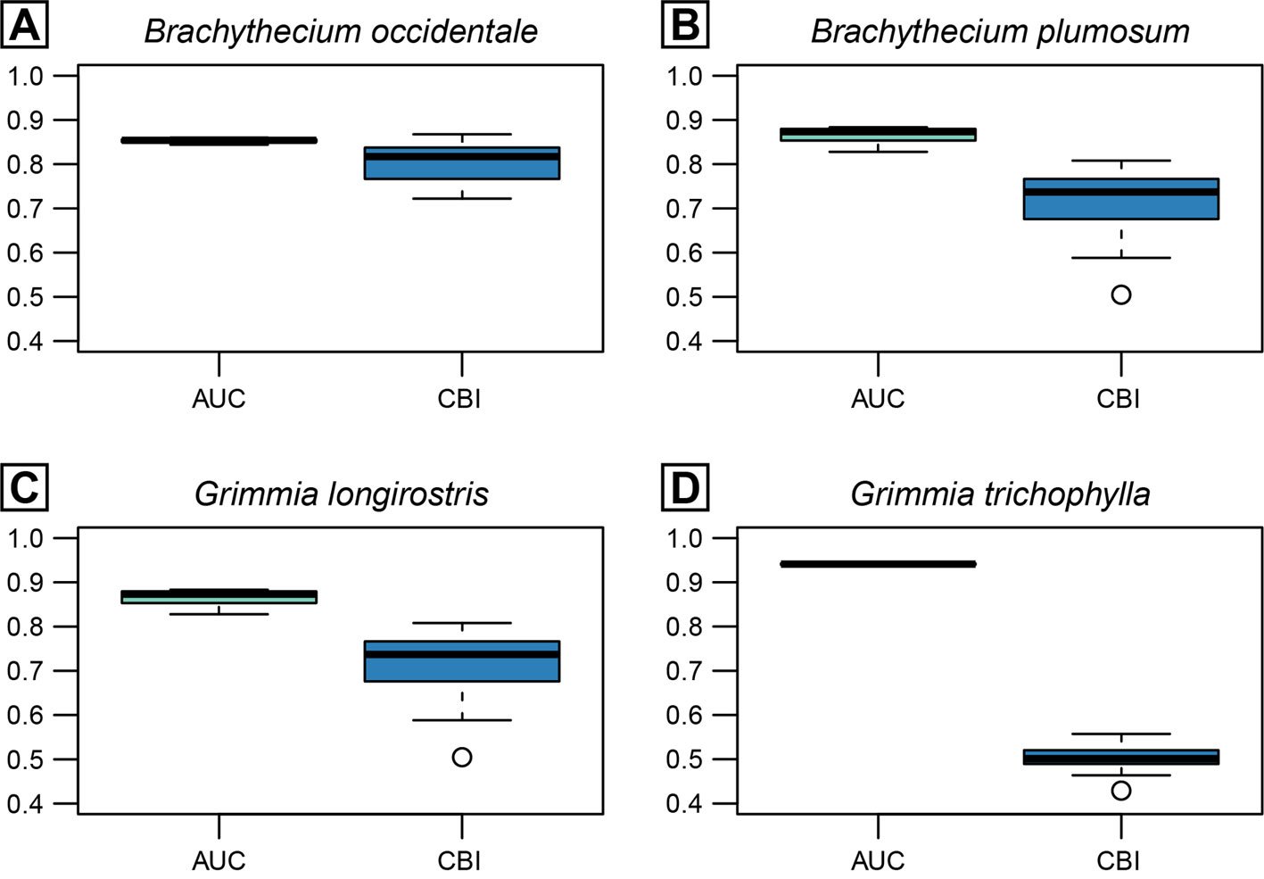
Table 3
Configuration of the best-performing Maxent model for each target species, along with the performance metrics from 5-fold cross-validation, including the area under the receiver operating characteristic curve (AUC) and the continuous Boyce Index (CBI). Feature class abbrev.: LQ, linear + quadratic; LQH, linear + quadratic + hinge.
| Species | Feature class | Regularization multiplier | AUC | CBI |
| Brachythecium occidentale | LQH | 2 | 0.83 | 0.82 |
| Brachythecium plumosum | LQ | 1 | 0.92 | 0.61 |
| Grimmia longirostris | LQ | 2 | 0.84 | 0.72 |
| Grimmia trichophylla | LQ | 1 | 0.94 | 0.73 |
Final models for all 4 species consistently included elevation, which emerged as the most influential predictor of the distribution of B. occidentale, G. longirostris, and G. trichophylla, yielding the highest gain in performance when used in isolation and causing the greatest drop when excluded from the model(Fig. 3). In contrast, B. plumosum was best predicted by BIO2 (Mean Diurnal Range), as evidenced by the greatest decrease in model performance when this predictor was omitted, with elevation playing a secondary but still relevant role. The remaining predictors retained in the final models showed only marginal contributions, including BIO2 and BIO3 (Isothermality) for B. occidentale, and slope and BIO2 for G. longirostris and G. trichophylla, respectively (Fig. 3). Regarding species response curves, elevation exhibited a positive sigmoidal relationship with environmental suitability across the 4 target species, with suitability values increasing with elevation (Supplementary material: Fig. 1). More specifically, all species showed an increase in predicted environmental suitability from intermediate values (0.5) at elevations between 2,000 m and 2,300 m to high suitability values (≥ 0.8) at elevations equal to or exceeding approximately 2,700 m, with their environmental optimum (asymptote) reached at elevations equal to or exceeding 2,600 m for both Brachythecium species and 3,200 m for the Grimmia species (Supplementary material: Fig. 1). On the other hand, BIO2 showed a reversed sigmoidal relationship with environmental suitability for B. plumosum, with suitability values decreasing as BIO2 values increased (Supplementary material: Fig. 1). Specifically, high environmental suitability values (≥ 0.8) were associated with BIO2 values of approximately ≤ 13 °C, with the environmental optimum (asymptote) occurring at BIO2 values ≤ 12.5 °C; environmental suitability for B. plumosum decreased to intermediate values (0.5) at BIO2 values equal to 14.5 °C (Supplementary material: Fig. 1).
Discussion
This contribution is based on previous proposals related to Mexican alpine mosses. The first concerns the degree of floristic similarity among mountain tops along the Neovolcanic Belt. The second is related to mosses distributed along lower sites or pathways that overcome, to some degree, the barrier effect of the mountain range.
Delgadillo (1971) and Mastretta-Yanes et al. (2015) introduced hypothetical considerations of the role of geological events on plant occupancy of highland areas. The sum effect of historical events and the ecological response of mosses are responsible for their distribution. Previous work proposed interchange and migration as the explanation for the floristic similarity across latitudes in the alpine areas of the Neovolcanic Belt (Delgadillo, 1971, 1987). In the revised list (Table 1), species common to mountain tops indicate certain degree of floristic similarity. Specifically, the Sørensen dissimilarity Index brings together Nevado de Colima and La Malinche (Supplementary material: Fig. 2), 2 distant areas with poor collecting records; Nevado de Toluca and Cofre de Perote are also geographically distant but their floristic similarity groups them together. A geographical similarity trend may not be demonstrated because alpine areas differ in size, collecting effort, and number of specimens available for comparison. By groups, however, the distribution of species in group G, groups C and C-E complement to cover the entire Belt. In group E, Bryoerythrophyllum bolivianum, Funaria orizabensis, Grimmia ovalis, Lepyrodon tomentosus, Rhytidium rugosum, and Syntrichia obtusissima are mainly known from the eastern mountains. In group W-C, Bryum pallescens and Orthodontium gracile are mainly distributed in western localities. The distribution gaps may fill out through additional field work, but if the pattern persists, it may indicate that interchange and migration have a directional trend.
Alpine moss species in central Mexico are found around 4,000 m in elevation (Table 1), but their range may exhibit a broad altitudinal interval (1,500- 2,000 m). Extreme low elevations are known for certain species (e.g., Anomobryum spp.), while others may be found as far high as 4,600-4,700 m (Grimmia montana). Most species in the alpine flora are acrocarpous and grow in tufts, cushions or mats inhabiting soil, humus or rocks. Among the frequent occupants of extreme habitats are species of Grimmia whose distribution may extend downwards in naturally open or disturbed spaces. Few pleurocarpous mosses occur in the alpine areas (Brachythecium, Leptodictyum, Leptopterigynandrum, and Sanionia) where they grow in mats (or tufts), on rocks or soil. By definition, epiphytism is an exceptional condition for mosses in the alpine environment and thus, contributes little to floristic similarity of extreme mountain tops; in protected enclaves, some trees or shrubs may still harbor species of Orthotrichum and Zygodon.
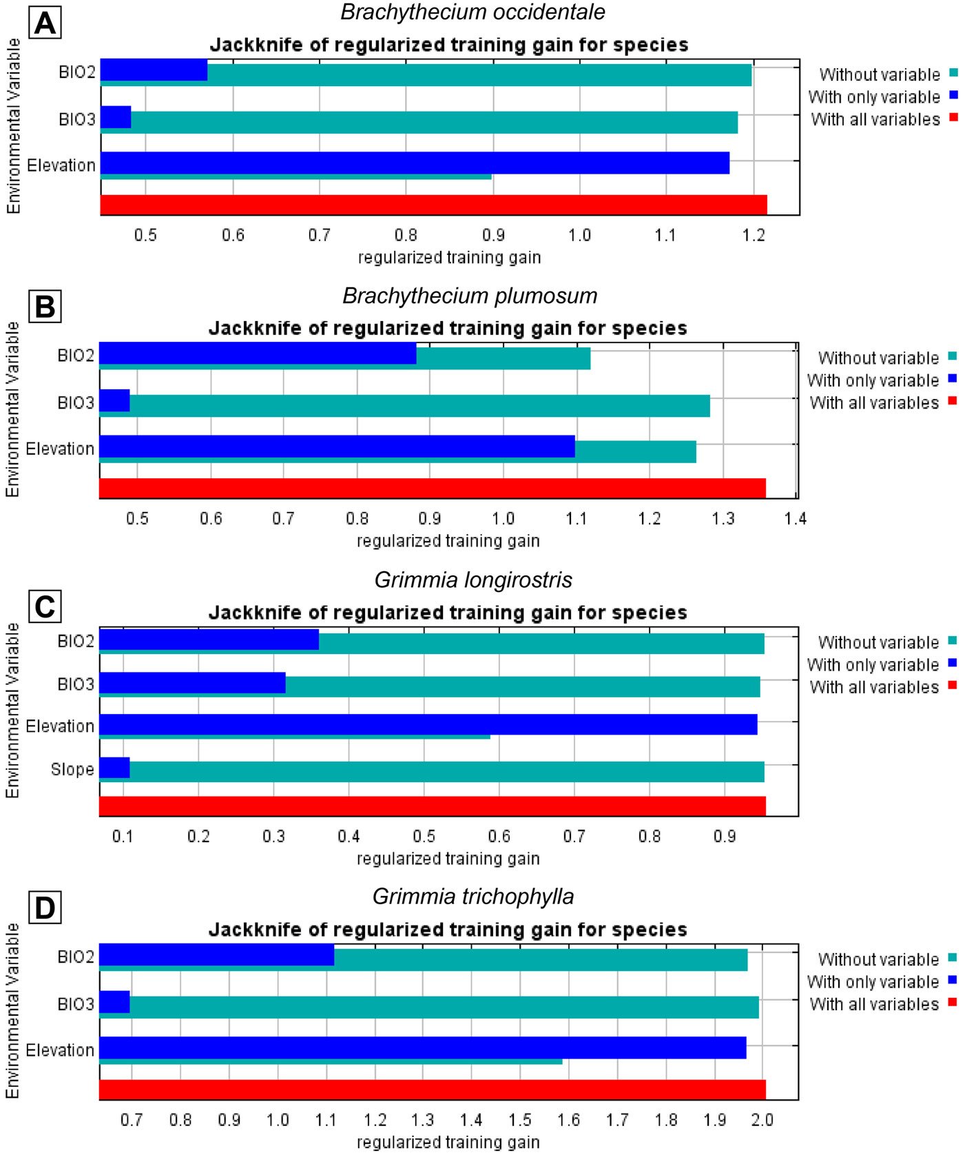
The barrier effect of the Neovolcanic Belt is not complete. Herbarium records indicate that there are alpine species present on either side of the mountain range that are also part of the flora in lower elevations. Results from SDMs show that Brachythecium and Grimmia are capable of inhabiting corridor elevations, mainly in central and eastern sites, with B. plumosum restricted to the easternmost corridor areas of the region (Fig. 2). These results confirm our corridor hypothesis and indicate that both acrocarpous and pleurocarpous mosses can move across mountain ranges; both are also known from lower dry habitats in northern states (Delgadillo-Moya & Peña-Retes, 2017; Sharp et al., 1994). Overall, elevation emerged as the dominant predictor of distribution of the 4 modeled alpine moss species, with a consistent sigmoidal increase of habitat suitability toward high elevations. Because elevation was strongly (negatively) correlated with multiple temperature-related bioclimatic variables (BIO1, BIO5, BIO6, BIO8–BIO11) and with Precipitation of Wettest Month (BIO13), our models effectively captured an integrated climatic signal via elevation. This pattern is expected along mountain altitude gradients where elevation systematically influences temperature and moisture regimes via orographic lifting (Franklin, 2010). Beyond elevation, the particular importance of BIO2 for predicting the distribution of B. plumosum, along with its negative sigmoidal relationship with predicted habitat suitability, suggests that this species may be particularly sensitive to fine-scale thermal fluctuations. The identification of these key predictors highlights the relevance of thermal and moisture constraints in shaping habitat suitability for the target mosses. Ecophysiological studies on the mechanisms underlying the effect of elevation on moss occurrence, for example through their photosynthetic responses are, however, still scarce and context-dependent (Wang et al., 2022).
In order to offset the barrier effect, displacement from other altitudes would require mosses to overcome ecological hindrances related to high insolation, temperature fluctuation, and water deficit that prevent successful occupation of exposed habitats in the highlands.
Acrocarpous moss growth has solved difficulties in the occupation and spread in alpine and highland areas. Since light for photosynthesis is not a limiting factor in the open habitats, water economy becomes critical for moss plants. It may move by capillary systems involving leaf arrangement and structure, and leaf papillae (cf. Proctor, 1979). These structures and stem aggregation, tomentum, and other structures present in cushions, compact turfs, and mats seem to reduce water loss. In the presence of hair points solar radiation and evaporation can be reduced by 20% or more in species of Tortula and Grimmia (Proctor, 1984). Pleurocarpous mosses such as Brachythecium, by comparison, occupy larger soil surfaces, and do not seem to cover large patches in the alpine area unless near a water source; exposed substrates in corridor areas may limit the spread of mosses that dry out rapidly.
Dispersal is a complex mechanism that seldomly cited for highland mosses. Numerous references may be consulted on the subject, with special reference to spores and other propagules that disperse mosses (for summaries, see Delgadillo & Pérez-Bandín, 1982; Richardson, 1981; Wyatt & Anderson, 1984). In general, the sporophytes in both acrocarpous and pleurocarpous taxa, whether apical or lateral, leave capsules exposed to wind for spore release. Spores liberated in air currents travel variable distances depending on atmospheric conditions, wind speed, spore size, survival, etc. Cleistocarpic species (Delgadillo, 1992) depend on other agents for spore liberation; spores may be released when capsule wall breaks down or is fractured during transportation by cattle hoofs.
Knowledge of the bryofloristic composition of the alpine environment of Mexico has improved, but deserves a finer evaluation; incidental fieldwork in the highlands still leads to discovery of new records (Cárdenas, 1989; Delgadillo, 2020; Greven, 1999; Yip, 2002). Current data offer a significant improvement of our understanding of this alpine moss flora and its distribution patterns, and highlight the usefulness of SDMs for hypothesis-driven ecological research. Specifically, SDMs allowed us to validate our hypothesis on corridor-based species interchange across mountain environments (Delgadillo, 1988, 1998), as well as in identifying key environmental variables shaping species distributions. Enhanced field exploration and ecological modelling research, both in alpine mountain tops and adjacent subalpine areas, could further improve our understanding of the actual distribution ranges of alpine mosses, as well as the mechanisms underpinning them.
Acknowledgements
Thanks are extended to two anonymous reviewers for criticism of a previous version of this article.
References
Aiello-Lammens, M. E., Boria, R. A., Radosavljevic, A., Vilela, B., & Anderson, R. P. (2015). spThin: an R package for spatial thinning of species occurrence records for use in ecological niche models. Ecography, 38, 541–545. https://doi.org/10.1111/ecog.01132
Bartram, E. B. (1945). Alpine mosses from Mexico. Revue Bryologique et Lichénologique, 15, 21–23.
Bartram, E. B. (1949). Alpine mosses from Mexico collected by Walter Kiener. The Bryologist, 52, 23–27.
Beaman, J. H. (1962). The Timberlines of Iztaccihuatl and Popocatepetl, Mexico. Ecology, 43, 377–385. https://doi.org/10.2307/1933367
Benito, B. (2023). “Collinear: R Package for Seamless Multicollinearity Management.” https://doi.org/10.5281/zenodo.10039489
Boyce, M. S., Vernier, P. R., Nielsen, S. E., & Schmiegelow, F. K. A. (2002). Evaluating resource selection functions. Ecological Modelling, 157, 281–300. https://doi.org/10.1016/S0304-3800(02)00200-4
Burnham, K. P., & Anderson, D. R. (2004). Multimodel inference: understanding AIC and BIC in model selection. Sociological Methods & Research, 33,261–304. https://doi.org/10.1177/0049124104268644
Cárdenas S. A. (1989). Nuevos registros para la flora de musgos de México y del Valle de México. Anales del Instituto de Biología, Universidad Nacional Autónoma de México, Serie Botánica, 58, 93–95.
Cardot, J. (1909a). Diagnoses préliminaires de mousses mexicaines. Revue Bryologique, 36, 67–77.
Cardot, J. (1909b). Diagnoses préliminaires de mousses mexicaines. Revue Bryologique, 36, 81–88.
Cardot, J. (1909c). Diagnoses préliminaires de mousses mexicaines. Revue Bryologique, 36, 105–115.
Cardot, J. (1910a). Diagnoses préliminaires de mousses mexicaines. Revue Bryologique, 37, 4–13.
Cardot, J. (1910b). Diagnoses préliminaires de mousses mexicaines. Revue Bryologique, 37, 49–59.
Cardot, J. (1910c). Diagnoses préliminaires de mousses mexicaines. Revue Bryologique, 37, 65–72.
Cardot, J. (1910d). Diagnoses préliminaires de mousses mexicaines. Revue Bryologique, 37, 117–128.
Cardot, J. (1911). Diagnoses préliminaires de mousses mexicaines. Revue Bryologique, 38, 1–9.
Cerrejón, C., Valeria, O., Mansuy, N., Barbé, M., & Fenton, N. J. (2020). Predictive mapping of bryophyte richness patterns in boreal forests using species distribution models and remote sensing data. Ecological Indicators, 119, 106826. https://doi.org/10.1016/j.ecolind.2020.106826
Cerrejón, C., Valeria, O., Muñoz, J., & Fenton, N. J. (2022). Small but visible: predicting rare bryophyte distribution and richness patterns using remote sensing-based ensembles of small models. Plos One, 17, e0260543. https://doi.org/10.1371/journal.pone.0260543
Conabio (Comisión Nacional para el Conocimiento y Uso de la Biodiversidad). (1997). Provincias biogeográficas de México. Retrieved April 19, 2024, from: http://www.conabio.gob.mx/informacion/gis/?vns=gis_root/region/biotic/rbiog4mgw http://geoportal.conabio.gob.mx/descargas/mapas/imagen/96/rbiog4mgw
Delgadillo, M. C. (1971). Phytogeographic studies on alpine mosses of Mexico. The Bryologist, 74, 331–346.
Delgadillo, M. C. (1984). Musgos alpinos de México: Cofre de Perote y Pico de Orizaba. Biótica, 9, 399–405.
Delgadillo, M. C. (1985). The Neovolcanic Belt of Mexico as a barrier and route of migration for mosses. Monographs in Systematic Botany from the Missouri Botanical Garden, 11, 41–44.
Delgadillo, M. C. (1987). Moss distribution and the phytogeographical significance of the Neovolcanic Belt of Mexico. Journal of Biogeography, 14, 69–78. http://dx.doi.org/10.2307/2844787
Delgadillo, M. C. (1988). Floristic corridors for moss distribution across the Neovolcanic Belt of Mexico. I. The Tuxpan corridor. Journal of Bryology,15,165–175. http://dx.doi.org/10.1179/jbr.1988.15.1.165
Delgadillo, M. C. (1992). Floristic corridors for moss distribution across the Neovolcanic Belt of Mexico. II. The cleistocarpic species. Journal of Bryology, 17, 313–316. http://dx.doi.org/10.1179/jbr.1992.17.2.313
Delgadillo, M. C. (1998). Floristic corridors for moss distribution across the Neovolcanic Belt of Mexico. III. The Michoacán corridors. Journal of Bryology,20, 27–39. http://dx.doi.org/10.1179/jbr.1998.20.1.27
Delgadillo, M. C. (2009). Floristic corridors for moss distribution across the Neovolcanic Belt of Mexico. IV. The Toluca and Chalco corridors. Journal of Bryology,31, 30-40. http://dx.doi.org/10.1179/174328209×404907
Delgadillo, M. C. (2015). Grimmia (Grimmiaceae, Bryophyta) in the Neotropics. Ciudad de México: Instituto de Biología, UNAM.
Delgadillo, M. C. (2020). Two disjunct moss species new to Mexico. Cryptogamie, Bryologie, 41, 83–87.
Delgadillo, M. C., Bello, B., & Cárdenas, S., A. (1995). LATMOSS, a catalogue of Neotropical mosses.
Monographs in Systematic Botany from the Missouri Botanical Garden, 56, 1–191.
Delgadillo, M. C., & Peña-Retes, A. P. (2017). Moss diversity in the state of Aguascalientes: revision and update.
Botanical Sciences, 95, 503–513. http://doi.org/10.17129/botsci.891
Delgadillo, M. C., & Pérez-Bandín, E. (1982). Spore liberation in mosses. I. Problems and perspectives of wind tunnel experiments. Cryptogamie: Bryologie et Lichénologie, 3, 39–49.
Dormann, C. F., Elith, J., Bacher, S., Buchmann, C., Carl, G., Carré, G. et al. (2012). Collinearity: a review of methods to deal with it and a simulation study evaluating their performance. Ecography, 36, 27–46. https://doi.org/10.1111/j.1600-0587.2012.07348.x
Fielding, A. H. & Bell, J. F. (1997). A review of methods for the assessment of prediction errors in conservation presence/absence models. Environmental Conservation, 24, 38–49. https://doi.org/10.1017/S0376892997000088
Franklin, J. (2010). Mapping species distributions: spatial inference and prediction. Cambridge: Cambridge University Press.
Freeman, E. A., & Moisen, G. G. (2008). A comparison of the performance of threshold criteria for binary classification in terms of predicted prevalence and kappa. Ecological Modelling, 217, 48–58. https://doi.org/10.1016/j.ecolmodel.2008.05.015
Gorelick, N., Hancher, M., Dixon, M., Ilyushchenko, S., Thau, D., & Moore, R. (2017). Google Earth Engine: planetary scale geospatial analysis for everyone. Remote Sensing of Environment, 202, 18–27. https://doi.org/10.1016/j.rse.2017.06.031
Greven, H. C. (1999). A synopsis of Grimmia in Mexico, including Grimmia mexicana, sp. nov. The Bryologist, 102, 426–436. https://doi.org/10.2307/3244231
Guillera-Arroita, G., Lahoz-Monfort, J. J., Elith, J., Gordon, A., Kujala, H., Lentini, P. E. et al. (2015). Is my species distribution model fit for purpose? Matching data and models to applications. Global Ecology and Biogeography, 24,276–292. https://doi.org/10.1111/geb.12268
Harrell, F. E., Lee, K. L., & Mark, D. B. (1996). Tutorial in biostatistics multivariable prognostic models: issues in developing models, evaluating assumptions and adequacy, and measuring and reducing errors. Statistics in Medicine, 15, 361–387. https://doi.org/10.1002/(SICI)1097-0258(19960229)15:4<361::AID-SIM168>3.0.CO;2-4
Hijmans, R. J., Barbosa, M., Ghosh, A., & Mandel, A. (2024). geodata: Download Geographic Data. R package version 0.6-2. https://CRAN.R-project.org/package=geodata
Hirzel, A. H., Le Lay, G., Helfer, V., Randin, C., & Guisan, A. (2006). Evaluating the ability of habitat suitability models to predict species presences. Ecological Modelling, 199, 142–152. https://doi.org/10.1016/j.ecolmodel.2006.05.017
Hooker, W. J. (1818). Musci Exotici; containing figures and descriptions of new or little-known foreign mosses and other cryptogamic subjects, Vol. 1. London: Longman, Hurst, Orme and Brown. https://doi.org/10.5962/bhl.title.10721
Hooker, W. J. (1820). Musci Exotici; containing figures and descriptions of new or little-known foreign mosses and other cryptogamic subjects, Vol. 2. London: Longman, Hurst, Orme and Brown. https://doi.org/10.5962/bhl.title.10721
Jiménez-Valverde, A., & Lobo, J. M. (2007). Threshold criteria for conversion of probability of species presence to either–or presence–absence. Acta Oecologica, 31, 361–369. https://doi.org/10.1016/j.actao.2007.02.001
Kass, J. M., Muscarella, R., Galante, P. J., Bohl, C. L., Pinilla-Buitrago, G. E., Boria, R. A. et al. (2021). ENMeval 2.0: Redesigned for customizable and reproducible modeling of species’ niches and distributions. Methods in Ecology and Evolution, 12,1602–1608. https://doi.org/10.1111/2041-210X.13628
Kutner, M. H., Nachtsheim, C. J., Neter, J., & Li, W. (2005). Applied linear statistical models, 5th Ed. Boston: McGraw-Hill.
Mastretta-Yanes, A., Moreno-Letelier, A., Piñero, D., Jorgensen, T. H., & Emerson, B. C. (2015). Biodiversity in the Mexican highlands and the interaction of geology, geography and climate within the Trans-Mexican Volcanic Belt. Journal of Biogeography, 42, 1586–1600. https://doi.org/10.1111/jbi.12546
Mateo, R. G., Felicisimo, A. M., & Muñoz, J. (2011). Species distributions models: a synthetic revision. Revista Chilena de Historia Natural, 84, 217–240. http://dx.doi.org/10.4067/S0716-078X2011000200008
Peduzzi, P., Concato, J., Kemper, E., Holford, T. R., & Feinstein, A. R. (1996). A simulation study of the number of events
per variable in logistic regression analysis. Journal of Clinical Epidemiology, 49, 1373–1379. https://doi.org/10.1016/S0895-4356(96)00236-3
Phillips, S. J., Anderson, R. P., Dudík, M., Schapire, R. E., & Blair, M. E. (2017). Opening the black box: an open-source release of Maxent. Ecography, 40, 887–893. https://doi.org/10.1111/ecog.03049
Phillips, S. J., Anderson, R. P., & Schapire, R. E. (2006). Maximum entropy modeling of species geographic distributions. Ecological Modelling, 190, 231–259. https://doi.org/10.1016/j.ecolmodel.2005.03.026
Phillips, S. J., & Dudík, M. (2008). Modeling of species distributions with Maxent: new extensions and a comprehensive evaluation. Ecography, 31, 161–175. https://doi.org/10.1111/j.2007.0906-7590.05203.x
Proctor, M. C. F. (1979). Structure and eco-physiological adaptation in bryophytes. In G. C. S. Clarke, & J. G. Duckett (Eds.), Bryophyte systematics (pp. 479–509). New York: Academic Press.
Proctor, M. C. F. (1984). Structure and ecological adaptation. In A. F. Dyer, & J. G. Duckett (Eds.), The experimental biology of bryophytes (pp. 9–37). New York: Academic Press.
R Development Core Team (2023). R: a language and environment for statistical computing. R Foundation for Statistical Computing, Vienna, Austria. https://www.R-project.org/
Richardson, D. H. S. (1981). Capsules and spore dispersal. In D. H. S Richardson (Ed.), The Biology of mosses (pp. 61–85). Oxford: Blackwell Scientific Publications.
Sharp, A. J, Crum, H., & Eckel, P. M. (Eds.). (1994). The moss flora of Mexico. Memoirs of the New York Botanical Garden, 69, 1–1113.
Thériot, I. (1921). Mousses du Mexique. Paris: Recueil des Publications de la Société Havraise D’Études Diverses.
Thériot, I. (1931). Quelques nouveautés bryologiques pour le Mexique.Travaux Cryptogamiques Dédiés à Louis Mangin, 7–10.
Thériot, I. (1933). Mexican mosses. IV. Revue Bryologique et Lichénologique, 5, 91–110.
Vanderpuye, A. W., Elvebakk, A., & Nilsen, L. (2002). Plant communities along environmental gradients of high-arctic mires in Sassendalen. Svalbard. Journal of Vegetation Science, 13, 875–884.
Wyatt, R., & Anderson, L. E. (1984). Breeding systems in bryophytes.In A. F. Dyer, & J. G. Duckett (Eds.), The experimental Biology of bryophytes (pp. 39–64). New York: Academic Press.
Wang, Z., Pi, C., Bao, W., & Bader, M. Y. (2022). Elevational trends in photosynthetic capacity and trait relationships of subtropical montane understorey bryophytes. Ecological Indicators,142, 109251. https://doi.org/10.1016/j.ecolind.2022.109251
Warren, D. L., & Seifert, S. N. (2011). Ecological niche modeling in Maxent: the importance of model complexity and the performance of model selection criteria. Ecological Applications, 21, 335–342. https://doi.org/10.1890/10-1171.1
Yip, K. L. (2002). Pseudephemerum, new to the United States and Mexico. The Bryologist, 105, 256–258.

Diversidad de cactáceas (Cactaceae: Caryophyllales) en Jalisco, México
Diversity of cacti (Cactaceae: Caryophyllales) in Jalisco, Mexico
Ulises Pinedo a, Mónica Carolina Báez-González a, Pedro González-Zamora b y Daniel Sánchez c, *
a Universidad de Guadalajara, Centro Universitario de Ciencias Biológicas y Agropecuarias, Departamento de Botánica y Zoología, Herbario Luz María Villarreal de Puga, Camino Ing. Ramón Padilla Sánchez 2100, 45200 Zapopan, Jalisco, México
b Grupo de Estudio de Cactáceas y Vida Silvestre del Occidente, A.C., Hacienda Nogueras s/n, 28454 Comala, Colima, México
c Universidad Nacional Autónoma de México, Instituto de Biología, Estación de Biología Chamela, Apartado postal 21, Km. 59 Melaque-Puerto Vallarta, 48980 Chamela, Jalisco, México
*Autor para correspondencia: dsanchez@ib.unam.mx (D. Sánchez)
Recibido: 12 septiembre 2025; aceptado: 26 enero 2026
Resumen
Cactaceae es un grupo diverso en las regiones áridas y semiáridas de México. La taxonomía de Cactaceae se ha reconfigurado en años recientes. En este trabajo se actualiza el listado de Cactaceae para Jalisco y analiza su distribución geográfica. Se construyó una base de datos con 1,894 registros. Se analizó la riqueza taxonómica y diversidad filogenética por diferentes criterios geográficos. El estudio reconoció 98 especies y 25 géneros nativos. Los géneros más diversos fueron Mammillaria y Opuntia. Se identificaron 6 zonas con alta riqueza taxonómica. Las celdas más diversas se ubicaron al noreste del estado, en los límites de los municipios Lagos de Moreno y Ojuelos, en la provincia Desierto Chihuahuense. En esta región, las condiciones de aridez son ideales para el establecimiento y diversificación de la familia. Las Tierras Bajas del Pacífico y Desierto Chihuahuense presentaron 59 y 56 especies, respectivamente. El bosque tropical caducifolio incluyó 86 especies. La región sur del estado con una marcada estación seca mostró una importante diversidad. Jalisco se ubicó en la octava posición de riqueza de cactáceas. Los resultados revelan la necesidad de complementariedad de diferentes regiones para lograr la conservación de este grupo de plantas.
Palabras clave: Bosque tropical caducifolio; Diversidad filogenética; Mammillaria; Riqueza taxonómica; Tierras Bajas del Pacífico
Abstract
Cactaceae is a diverse group in the arid and semi-arid regions of Mexico. Taxonomy of Cactaceae has been reconfigured in recent years. This work aims to update the list of Cactaceae for Jalisco and analyze their geographical distribution. A database with 1,894 records was built. Taxonomic richness and phylogenetic diversity were analyzed using different geographical criteria. The study recognized 98 native species and 25 genera. The most diverse genera were Mammillaria and Opuntia. Six zones with high richness were identified. The most diverse cells are located in the northeast of the state, at the limits of the municipalities of Lagos de Moreno and Ojuelos in the Chihuahuan Desert province. Those cells in northeastern Jalisco concentrated the highest richness, where arid conditions are ideal for the establishment and diversification of the family. The southern region of the state, with a marked dry season, showed significant diversity. The Pacific Lowlands and the Chihuahuan Desert presented 59 and 56 species, respectively. Meanwhile, the tropical deciduous forest included 86 species. Those results ranked Jalisco in the eighth position in cactus richness. The results highlight the need for complementary conservation efforts across different regions to protect this plant group.
Keywords: Tropical deciduous forest; Phylogenetic diversity; Mammillaria; Taxonomic richness; Pacific lowlands
Introducción
La familia Cactaceae es un elemento florístico distintivo de los paisajes áridos y semiáridos de México (Bravo-Hollis, 1978). Cactaceae es un grupo monofilético caracterizado por la presencia de brotes cortos altamente especializados o areolas, tallos u hojas suculentas, hojas modificadas como espinas y metabolismo CAM (Gibson y Nobel, 1986; Mauseth, 2006; Nyffeler, 2002). El origen de la familia es estimado en ca. de 30 Ma en el continente americano (Arakaki et al., 2011). Los cactus se han diversificado en diferentes hábitats, principalmente en regiones áridas y semiáridas del continente y en menor medida en el dosel de los bosques neotropicales (Anderson, 2001).
De acuerdo con Guzmán et al. (2003), la familia se compone en México de 63 géneros y 669 especies, de las cuales ca. 70% son endémicas. En la flora de México, Cactaceae se encuentra en la quinta posición por su diversidad de especies (Villaseñor, 2003). La región central y norte del país es considerada como un centro de diversificación de cactáceas (Mutke et al., 2015). Godínez-Álvarez y Ortega-Baes (2007) reconocieron 8 estados mexicanos con más de 100 especies de cactus. Sin embargo, este listado no es preciso dada la complejidad taxonómica de la familia (González-Elizondo et al., 2017).
Listados dirigidos a cactáceas han sido desarrollados en Mazapil, Zacatecas (Signoret y Hernández, 2010), Tehuacán-Cuicatlán (Arias et al., 2012) y el Bajío y zonas adyacentes (Arias y Aquino, 2019; Arias et al., 2024). Sobresalen los análisis de riqueza y endemicidad de cactáceas de Durango (González-Elizondo et al., 2017), Tamaulipas (García-Morales et al., 2022) y el Bajío y regiones adyacentes (Aquino et al., 2025). Mutke et al. (2015) sugieren que Jalisco representa un centro de diversidad secundario para Cactaceae. Listados previos para la familia reconocen para Jalisco 25 géneros y 87 especies (Guzmán et al., 2003), 27 géneros y 134 especies (Ramírez-Delgadillo et al., 2010), 33 géneros y 135 especies (Villaseñor, 2016) y 27 géneros y 110 especies (Arreola-Nava y Ramírez-Ulloa, 2017).
En los últimos años, los análisis filogenéticos y morfométricos han reconfigurado la taxonomía de la familia (Korotkova et al., 2021). También, se han descrito nuevas especies de cactáceas para Jalisco (e.g., González-Zamora et al., 2020, 2021; Ortiz-Brunel et al., 2023). Los análisis biogeográficos son herramientas importantes en la conservación ya que permiten identificar regiones con alta diversidad. Por lo tanto, este estudio busca actualizar el listado de géneros y especies de cactáceas de Jalisco, analizar la distribución de la diversidad taxonómica y filogenética, y comparar la riqueza taxonómica y diversidad filogenética de las cactáceas de Jalisco en relación con otros estados con una alta diversidad de cactáceas.
Materiales y métodos
Jalisco se encuentra en el occidente central de México y comprende 78,595.9 km2 (INEGI, 2022) (fig. 1). El estado tiene 2 estaciones pluviales bien definidas, pero no estaciones termales marcadas (Rzedowski y McVaugh, 1966). Jalisco incluye 7 tipos de vegetación, bosque de coníferas y encinos (BCE), bosque espinoso (BE), bosque mesófilo de montaña (BMM), bosque tropical caducifolio (BTC), bosque tropical subcaducifolio (BTS) y matorral xerófilo (MX) (Rzedowski, 1978) (fig. 1C). Además, en Jalisco convergen 6 provincias biogeográficas, Cuenca del Balsas (CB), Desierto Chihuahuense (DCh), Faja Volcánica Transmexicana (FVT), Sierra Madre del Sur (SMS), Sierra Madre Occidental (SMOc) y Tierras Bajas del Pacífico (TBP) (Morrone et al., 2017) (fig. 1D). El estado cuenta con 125 municipios, los cuales están agrupados en 12 regiones administrativas que facilitan la gobernanza y desarrollo (IIEG, 2025) (fig. 1B). La riqueza de plantas vasculares en Jalisco, lo coloca en el cuarto estado con mayor diversidad vegetal en México (Gudiño-Cano et al., 2025).
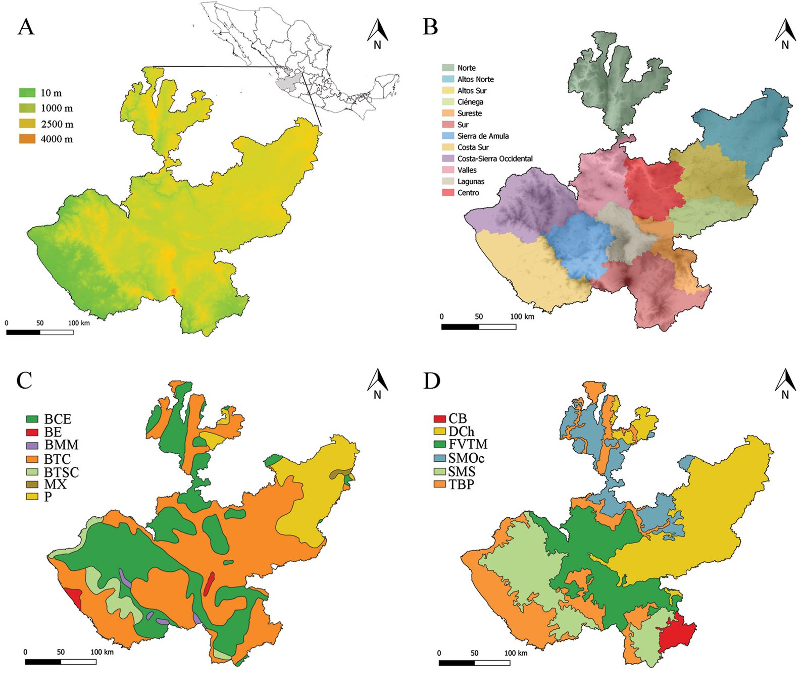
Para la construcción de este listado, comparamos las listas de cactáceas publicadas por Arreola-Nava (1990), Guzmán et al. (2003), Ramírez-Delgadillo et al. (2010), Villaseñor (2016) y Arreola-Nava y Ramírez-Ulloa (2017). También, realizamos una revisión de los especímenes de los herbarios IBUG, IEB, MEXU y ZEA (Thiers, 2025), así como la integración de algunos registros de las plataformas SEINeT (2024) e iNaturalist (2024). La taxonomía fue estandarizada con el listado revisado de Cactaceae (Korotkova et al., 2021), estudios taxonómicos recientes (González-Zamora et al., 2020, 2021; Ortiz-Brunel, 2025; Ortiz-Brunel et al., 2023) y algunos ajustes en el complejo de especies de Mammillaria jaliscana Boed. Los nombres de las especies y sus autoridades son citados de acuerdo con el “International Plant Names Index” (IPNI, 2025). Este listado se complementó con el estado de conservación de la Unión Internacional para la Conservación de la Naturaleza (IUCN, 2012) y la PROY-NOM-059-SEMARNAT-2025 (Semarnat, 2025).
Con base en el listado taxonómico, corroboramos, corregimos y/o determinamos ejemplares de los herbarios previamente citados. Así mismo, construimos una base de datos electrónica que incluyó latitud y longitud contenida en las etiquetas, o bien las georreferencias estimadas con Google Earth Pro (Google, 2022) para aquellos especímenes que no presentaron esta información. Posteriormente, para completar la base de datos para el análisis, proyectamos los puntos de presencia en el programa QGIS 3.2.2-Bonn (QGIS, 2025) usando el sistema de coordenadas geográficas WGS84 sobre el polígono de Jalisco (INEGI, 2022) y con las capas de división municipal (INEGI, 2022), modelo digital de elevación (U.S. Geological Survey, 2024), tipo de vegetación (INEGI, 1990) y provincias biogeográficas (Morrone, 2017).
Se construyó una matriz binaria (ausencia/presencia) con las especies que habitan los 16 estados de México más diversos en cactáceas de acuerdo con el catálogo de cactáceas mexicanas (Guzmán et al., 2003), el análisis presentado por Godínez-Álvarez y Ortega-Baes (2007) y los listados actualizados para Durango (González-Elizondo et al., 2017) y Tamaulipas (García-Morales et al., 2022), acotado a la taxonomía de Cactaceae propuesta por Korotkova et al. (2021).
Con la intención de tener un árbol filogenético más completo, respecto a otras fuentes, se descargaron de GenBank (NCBI, 2024) las secuencias trnK/matK, psbA-trnH, rpl16 y trnL-trnF para las especies que conformaron la matriz de los estados más diversos en cactáceas. La matriz de cada secuencia fue alineada en MAFFT (Katoh y Standley, 2013), ajustada manualmente y finalmente concatenadas con las otras matrices individuales. Se realizó un análisis filogenético de inferencia Bayesiana con BEAST v. 2.7.3 (Bouckaert et al., 2019). El análisis fue particionado y usó el modelo GTR + G, el cual consistió en 2 corridas independientes de 4 cadenas y 10 millones de iteraciones, guardando un árbol cada 1,000 generaciones. Debido a que no todas las especies presentan el mismo número de secuencias, se forzó la monofilia de las tribus, las cuales han sido previamente corroboradas como grupos naturales, Opuntieae (Griffith y Porter, 2009), Cylindropuntieae (Griffith y Porter 2009), Cacteae (Vázquez-Sánchez et al., 2013), Cereeae (Romeiro-Brito et al., 2023), Echinocereeae (Sánchez et al., 2014), e Hylocereeae (Korotkova et al., 2017). Finalmente, aquellas especies sin ninguna secuencia disponible, fueron agregadas como ramas colapsadas dentro del género correspondiente.
La base de datos de los cactus de Jalisco y el árbol filogenético se usaron para estimar la riqueza taxonómica y la diversidad filogenética por cuadrícula (tamaño 0.333°), altitud, división municipal, tipo de vegetación y provincia biogeográfica mediante el programa Biodiverse (Laffan et al., 2010). Finalmente, se calculó la diversidad filogenética por estado con la matriz binaria de las entidades más diversas en cactáceas y el árbol filogenético con el software Picante ver. 1.6 (Kembel et al., 2010) en el programa R (R Core Team, 2024).
Resultados
Con base en los registros revisados, se listan para Jalisco a 102 especies agrupadas en 25 géneros (apéndice). Cada especie es citada por un ejemplar de respaldo preservado en alguno de los herbarios nacionales o internacionales (apéndice). Cuatro especies fueron reconocidas como plantas cultivadas, por lo que, solo 98 fueron incluidas en los análisis. Mammillaria Haw. resultó el género más diverso con 24 especies, seguido de Opuntia Mill. con 18, Selenicereus (A.Berger) Britton et Rose con 8 y Acanthocereus (Engelm.) Britton et Rose con 7 (apéndice, figs. 2, 3). La base de datos incluyó 1,898 registros, entre los cuales destacan algunas especies representadas por solo 1 registro (e.g., Acanthocereus atropurpureus, Backebergia militaris, Selenicereus dorschianus) y hasta por 176 en Stenocereus queretaroensis. Los registros de los especímenes se encontraron desde nivel del mar, como Cochemiea mazatlanensis y Stenocereus standleyi hasta 2,995 m de altitud como Disocactus speciosus y Opuntia robusta. La mayor riqueza de especies se concentró entre 1,500 y 2,250 m snm, con 59 especies. Por otro lado, algunas especies se encontraron en solo 1 municipio (e.g. Acanthocereus paradoxus en Tolimán, Coryphantha tripugionacantha y Echinocereus spinigemmatus en Huejuquilla el Alto, Kimnachia ramulosa en Talpa de Allende), mientras que Stenocereus queretaroensis y Mammillaria scrippsiana habitan 51 y 31 municipios, respectivamente (apéndice). Finalmente, 7 especies son endémicas de Jalisco, Acanthocereus atropurpureus, A. paradoxus, Mammillaria arreolae, M. limonensis, M. manana, Opuntia setocarpa y Selenicereus dorschianus (apéndice).
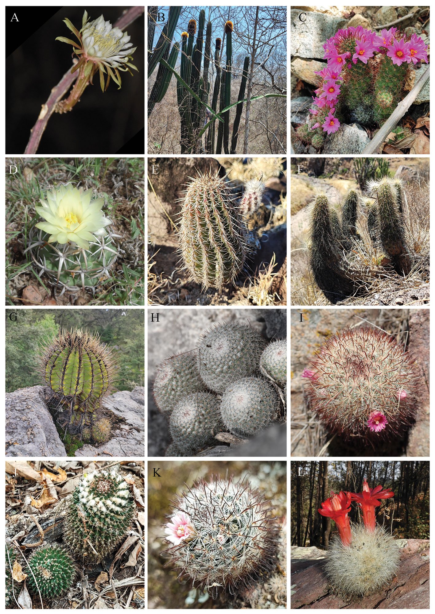
Los 16 estados más diversos en cactáceas compilaron 570 especies (material suplementario 1). Las especies mayormente distribuidas fueron Cylindropuntia imbricata, Myrtillocactus geometrizans y Opuntia pubescens en 13 estados, seguidas por Cylindropuntia kleiniae (DC.) F.M.Knuth, Cylindropuntia leptocaulis (DC.) F.M.Knuth y Mammillaria uncinata en 12 estados. Por otro lado, el árbol filogenético recuperó todos los géneros como grupos monofiléticos. La topología detallada es mostrada en el material suplementario 2.
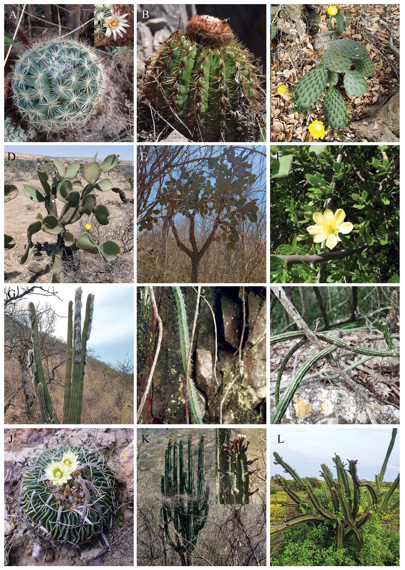
La riqueza taxonómica (RT) por cuadrícula mostró 3 celdas con los valores más altos en la región Altos Norte al noreste de Jalisco (fig. 4A, con 29, 23 y 23 especies). También, celdas con valores moderados de RT (fig. 4A) se encontraron en las regiones Norte (16 especies), Centro (20 y 18 especies), Sur (17 y 16 especies), Sierra de Amula (17 especies) y Costa Sur (16 especies) (fig. 4A). En cuanto a la diversidad filogenética (DF), el análisis también recuperó 3 celdas con los valores más altos en la región Altos Norte (DF 299-309) (fig. 4B). Este último análisis recupera celdas con altos valores de DF en las regiones Norte (DF 207-234), Centro (DF 249-269), Lagunas (DF 254), Sur (DF 264), Sierra de Amula (DF 258-286) y Costa Sur (DF 238) (fig. 4B).
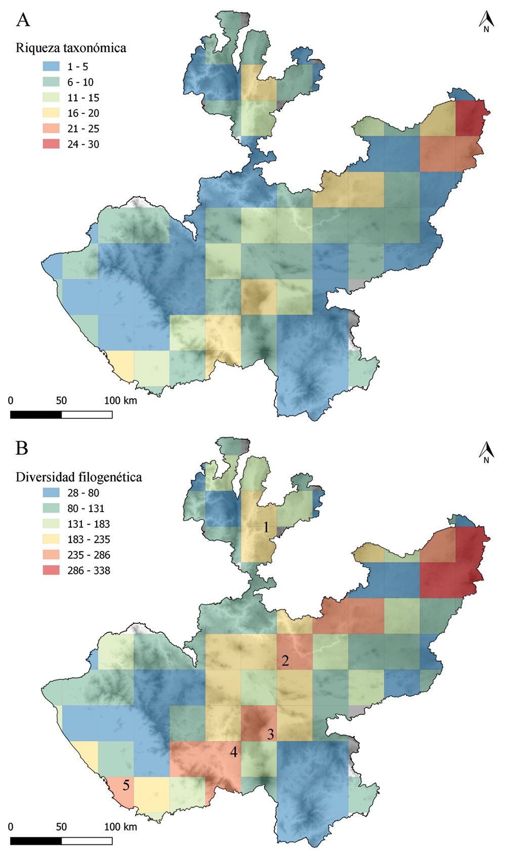
Los municipios con la mayor DF están asociados a las celdas con alta riqueza. Lagos de Moreno es el municipio más diverso con 34 especies; los 10 municipios con mayor RT y DF aparecen listados en la tabla 1. Por otra parte, el bosque tropical caducifolio se mostró como la vegetación con mayor riqueza de cactáceas en Jalisco con 79 especies, así como el valor más alto de DF (tabla 2). Mientras que las Tierras Bajas del Pacífico y el Desierto Chihuahuense resultaron las provincias con mayor diversidad de cactáceas con 59 y 56 especies, respectivamente, así mismo, presentan la misma relación en sus valores de DF (tabla 3). Finalmente, San Luis Potosí resultó el estado con los valores más altos de RT, seguido por Tamaulipas y Durango (tabla 4). Mientras que Jalisco obtuvo la octava y décima posición, de acuerdo con respectivos valores de RT y DF (tabla 4).
| Municipio | RT | DF |
|---|---|---|
| Lagos de Moreno | 34 | 402 |
| Ojuelos de Jalisco | 29 | 338 |
| Mezquitic | 21 | 296 |
| Cuautitlán de García Barragán | 19 | 261 |
| La Huerta | 18 | 254 |
| Yahualica de González Gallo | 17 | 253 |
| Tolimán | 15 | 260 |
| Autlán de Navarro | 14 | 244 |
| Bolaños | 14 | 221 |
| Villa Hidalgo | 14 | 198 |
| Zapopan | 14 | 237 |
| Cabo Corrientes | 13 | 214 |
| Amacueca | 12 | 201 |
| Tecolotlán | 12 | 215 |
| Atoyac | 11 | 191 |
| Encarnación de Díaz | 11 | 175 |
| Tepatitlán de Morelos | 11 | 168 |
| Tomatlán | 11 | 196 |
| Tipo de vegetación | RT | DF |
|---|---|---|
| Bosque tropical caducifolio | 79 | 680 |
| Bosque de coníferas y encinos | 50 | 500 |
| Pastizal | 42 | 471 |
| Matorral xerófilo | 21 | 270 |
| Bosque espinoso | 17 | 283 |
| Bosque tropical subcaducifolio | 11 | 154 |
| Bosque mesófilo de montaña | 2 | 31 |
| Provincia biogeográfica | RT | DF |
|---|---|---|
| Tierras Bajas del Pacífico | 59 | 612 |
| Desierto Chihuahuense | 56 | 554 |
| Sierra Madre Occidental | 37 | 421 |
| Faja Volcánica Transmexicana | 32 | 392 |
| Sierra Madre del Sur | 30 | 357 |
| Cuenca del Balsas | 6 | 94 |
| Estado | RT | DF |
|---|---|---|
| San Luis Potosí | 150 | 1,179 |
| Tamaulipas | 131 | 1,064 |
| Coahuila | 126 | 940 |
| Durango | 124 | 1,033 |
| Nuevo León | 123 | 963 |
| Oaxaca | 111 | 903 |
| Zacatecas | 104 | 954 |
| Jalisco | 98 | 811 |
| Querétaro | 95 | 891 |
| Sonora | 95 | 794 |
| Guanajuato | 90 | 829 |
| Hidalgo | 79 | 782 |
| Chihuahua | 79 | 741 |
| Puebla | 76 | 745 |
| Michoacán | 61 | 599 |
| Guerrero | 58 | 569 |
Discusión
Este trabajo permitió reconocer 102 especies de cactáceas para Jalisco agrupadas en 25 géneros. De las cuales, 4 especies están documentadas como altamente cultivadas en el país (Epiphyllum phyllanthus, Opuntia cochenillifera, O. ficus-indica, O. undulata; apéndice). Mammillaria y Opuntia fueron los géneros más diversos para Jalisco, lo cual coincide con lo reportado para Durango (González-Elizondo et al., 2017), Tamaulipas (García-Morales et al., 2022), el Bajío y regiones adyacentes (Aquino et al., 2025). Ambos géneros son comúnmente reconocidos como elementos de gran diversidad e importancia para México.
El catálogo de cactáceas mexicanas sugiere 87 especies para Jalisco y representa la propuesta más conservadora para el estado (Guzmán et al., 2003). Mientras que Ramírez-Delgadillo et al. (2010) y Villaseñor (2016) reconocieron a 135 especies de cactáceas para Jalisco, un número de especies sobreestimado para el estado. Para estos últimos listados, destacan la inclusión de Ferocactus pilosus (Galeotti) Werderm., Lophophora williamsii (Lem. ex J.F.Cels) J.M.Coult. y 4 especies de Turbinicarpus (Backeb.) Buxb. et Backeb., especies que habitan los suelos calizos del Desierto Chihuahuense y la Sierra Madre Oriental, suelos que no tienen representación en la porción noreste de Jalisco.
El presente trabajo destaca porque cada una de las 102 especies reconocidas están respaldadas por un ejemplar de herbario (apéndice). Recientemente, el inventario de la flora de Jalisco incluyó un listado de Cactaceae (Gudiño-Cano et al., 2025), con base en los resultados preliminares de la tesis del primer autor (González-Pinedo, 2024). Sin embargo, el listado de Gudiño-Cano et al. (2025) retoma especies que representan especímenes con una localidad errónea o mal determinados. Por ejemplo, los autores incluyeron a Cylindropuntia leptocaulis, L. N. Gooding 1377 (NY 3889154), anotado con la localidad La Cienega y registrado como La Ciénega, Jalisco en la base de datos del herbario NY. Sin embargo, otros especímenes colectados por L. N. Gooding con números de colecta muy cercanos, en la misma fecha y en la misma localidad como Stenocereus thurberi (L. N. Gooding 1374, NY), Echinocereus engelmannii (L. N. Gooding 1378, NY) y Lophocereus schottii (L. N. Gooding 1381, NY), este último anotado como La Cienega, Sonora, son especies representativas del matorral sonorense y nunca han sido colectadas en Jalisco. Por otro lado, Stenocereus chrysocarpus fue registrado en la Estación de Biología Chamela, La Huerta, Jalisco con el ejemplar A. Domínguez M. 846 (MEXU). No obstante, el trabajo de campo realizado en la Estación de Biología Chamela y regiones adyacentes, sugieren que dicha especie fue confundida con S. fricii, una especie común en la costa del occidente de México. Mientras que S. chrysocarpus es un taxón restringido a la Cuenca del Balsas.
En este trabajo reconocemos a las 2 subespecies de Mammillaria jaliscana (Korotkova et al., 2021) como especies distintas. Por un lado, M. jaliscana agrupa a plantas con 4-8 espinas centrales, sin cerdas axilares, flores magenta y que habitan laderas rocosas del bosque de encino en el centro y norte de Jalisco (Britton y Rose, 1923). Mientras que M. zacatecasensis incluye plantas con 3-4 espinas centrales, sin cerdas axilares, flores con tépalos amarillo pálido a rosa claro, que habitan los pastizales y su ecotono con el matorral xerófilo en Zacatecas, Aguascalientes, Guanajuato y noroeste de Jalisco (Shurly, 1960). Plantas con estas características han sido relacionadas al nombre M. rettigiana Boed. (Boedecker, 1930), una planta con una descripción no detallada y una localidad tipo sin precisión, señalada simplemente como al SO de Hidalgo, región en donde no ha sido colectado algún espécimen con las características previamente señaladas. Por otra parte, Mammillaria gilensis Boed. ha sido incluida como sinónimo de M. rettigiana (Korotkova et al., 2021) o M. crinita (Lüthy, 1995); sin embargo, un análisis filogenético reciente corrobora a M. gilensis Boed. como un linaje independiente cercano a Mammillaria bocasana Poselg. (Ortiz-Brunel, 2025). En este sentido, se sugiere el uso de M. zacatecasensis sobre M. rettigiana y la validación de M. gilensis como especie distinta.
Los análisis de riqueza taxonómica y diversidad filogenética mostraron los valores más altos en el extremo noreste del estado (fig. 4), en la región de los Altos Norte, en los municipios Lagos de Moreno y Ojuelos de Jalisco (tabla 2). Estas celdas, con índices más altos, se ubican en una región en donde predomina el pastizal y el matorral xerófilo. Los géneros Mammillaria, Opuntia, Echinocereus Engelm. y Stenocactus (K.Schum.) A.Berger están bien representados en este tipo de vegetación (apéndice, figs. 2, 3). Esta región se incluye en el Desierto Chihuahuense, una región considerada como un centro de diversidad y endemismo para la familia (Hernández et al., 2004). El clima dominante en esta región es semiárido (BS) (Rzedowski, 1978), lo cual coincide con el análisis de las cactáceas de Durango, en donde las celdas con mayor número de especies se presentan en las zonas áridas y semiáridas del estado (González-Elizondo et al., 2017). El bosque tropical caducifolio resultó el tipo de vegetación con mayor RT. Este tipo de vegetación es el más abundante en el estado y está presente en muchas de las celdas secundarias de diversidad (fig. 4B). El clima de esta región incluye climas cálidos subhúmedos a semicálidos con lluvias en verano (Aw) (Rzedowski, 1978). Rzedowski y Calderón-de Rzedowski (2013) destacan a Cactaceae en el séptimo lugar de las familias mejor representadas en el bosque tropical caducifolio en México, un linaje bien adaptado al periodo seco de los bosques estacionales. En el bosque tropical caducifolio destacan las cactáceas columnares de la tribu Echinocereeae, así como los géneros Mammillaria, Acanthocereus, Selenicereus (apéndice, figs. 2, 3).
En el presente análisis destaca la cantidad de celdas secundarias con altos valores de DF. Estas celdas secundarias están asociadas a la heterogeneidad ambiental y edáfica. El grupo de celdas 1 (fig. 4B), región Norte del estado, se ubica en una zona de transición entre el Desierto Chihuahuense, la Sierra Madre Occidental y las Tierras Bajas del Pacífico e incluye vegetación y ecotonos de bosque de coníferas y encinos, bosque tropical caducifolio y pastizal. Esta región del municipio de Mezquitic y zonas adyacentes a Bolaños y Huejuquilla el Alto es particularmente vulnerable debido a que existen pocas áreas destinadas para la conservación (Semadet, 2025). La celda 2 (fig. 4B), ubicada en la región Centro, particularmente en los límites de la Zona Metropolitana de Guadalajara, incluye zonas de transición entre el bosque de coníferas y encino y el bosque tropical caducifolio. Por lo que destacan la importancia del Área de Protección de Flora y Fauna La Primavera y los bosques urbanos como la Barranca de Huentitán, el Diente y Huaxtla. La celda 3 (fig. 4B), en la región Lagunas, denota la importancia de la conservación de la biodiversidad en la sierra de Tapalpa. Esta celda incluye bosque de coníferas, encinos y cañadas con ecotonos con el bosque tropical caducifolio. En este sentido, el Paisaje Biocultural Sierra Volcánica (Rainforest Alliance Mexico, 2024) provee una oportunidad para fomentar el desarrollo sostenible en la región.
Por otra parte, el grupo de celdas 4 (fig. 4B), en las regiones Sierra de Amula y Sur, en los límites de la Sierra Madre del Sur y su transición con las Tierras Bajas del Pacífico, expone la diversidad biológica que alberga la Reserva de la Biosfera Sierra de Manantlán. Esta área natural brinda servicios ecosistémicos a una región de Jalisco y Colima. Sin embargo, la región presenta una fuerte complejidad sociopolítica, por lo que la gestión debe integrar la conservación ambiental y el desarrollo social (Graf et al., 2003). Finalmente, la celda 5 en la región Costa Sur, representa la celda asociada a la Reserva de la Biosfera Chamela-Cuixmala y la Estación de Biología Chamela, Instituto de Biología, UNAM (EBCh), que, si bien no presenta un alto grado de heterogeneidad ambiental, representa una porción de bosque tropical caducifolio bien conservado y documentado con una gran diversidad vegetal (Lott y Atkinson, 2006). Particularmente, la EBCh destaca como centro de investigación y enseñanza, por lo que representa una oportunidad para estudiar la diversidad morfológica, demografía e interacciones de las cactáceas que alberga la reserva.
La riqueza taxonómica aquí reportada coloca a Jalisco en la octava posición de los estados más diversos en cactáceas. De acuerdo con Godínez-Álvarez y Ortega-Báez (2007), Jalisco forma parte de los estados más diversos en este grupo de plantas y representa uno de 8 estados que en su conjunto albergan 80% de la diversidad de la familia. Mientras que, el valor de diversidad filogenética lo reubica en el décimo lugar. Contrario a ésto, Coahuila presentó 126 especies, el tercer lugar, seguido de Durango con 124 especies. Sin embargo, Durango mostró un valor más alto de diversidad filogenética (tabla 4). Miller et al. (2018) sugieren usar complementariamente ambos valores en los estudios de biodiversidad. En este trabajo, ambos valores, RT y DF se correlacionan con los criterios geográficos analizados para Jalisco (tablas 1, 2, 3; fig. 4). Sin embargo, el análisis de DF por cuadrícula recupera y revela celdas secundarias de diversidad, que no se recuperan con claridad en los análisis de RT. Este hecho también es observado en los patrones de distribución de la diversidad de plantas vasculares en la Sierra Madre del Sur (Aragón-Parada et al., 2023).
Las 98 especies nativas del estado de Jalisco representan 15% de la diversidad de la familia en el país. La alta diversidad de cactáceas de Jalisco resulta del conjunto de especies que habitan las regiones semiáridas en el noroeste del estado, en los pastizales y matorrales que se incluyen en el Desierto Chihuahuense, y de las especies que se encuentran en las regiones cálido-húmedas del bosque tropical caducifolio, ubicados principalmente en las Tierras Bajas del Pacifico y, en menor medida, de las especies en regiones templadas de los bosques de coníferas y encinos de la Faja Volcánica Transmexicana y la Sierra Madre del Sur. Este trabajo denota el papel de la estacionalidad en la diversidad de cactáceas en el bosque tropical caducifolio y muestra zonas concretas de alta diversidad que deben ser incluidas o mantenidas en el conjunto de áreas naturales protegidas de Jalisco.
Agradecimientos
Los autores agradecemos a los curadores y técnicos de los herbarios IBUG, IEB, MEXU y ZEA por facilitar la consulta de sus especímenes. También a Azul Martínez Poiré y David Gómez Quintero por su ayuda en el trabajo de campo. DS agradece a David Aquino y Juan Pablo Ortíz Brunel por el intercambio de opiniones e ideas. Este trabajo honra la memoria de Hilda Julieta Arreola Nava, apasionada estudiosa de las cactáceas del occidente de México. Los autores apreciamos los comentarios de dos revisores anónimos.
Apéndice
Apéndice. Listado de las especies de Cactaceae aceptadas en este trabajo y su distribución por diferentes criterios. Las especies endémicas de Jalisco se indican con doble asterisco (**), las especies cultivadas se indican en negritas. División municipal clave INEGI (2022). Tipo de vegetación (Rzedowski, 1978, 1990), BCE: bosque de coníferas y encinos, BE: bosque espinoso, BMM: bosque mesófilo de montaña, BTC: bosque tropical caducifolio, BTS: bosque tropical subcaducifolio; MX: matorral xerófilo, P: pastizal. Provincia biogeográfica (Morrone, 2017), CB: Cuenca del Balsas, DCh: Desierto Chihuahuense, FVT: Faja Volcánica Transmexicana, SMOc: Sierra Madre Occidental, SMS: Sierra Madre del Sur, TBP: Tierras bajas del Pacífico. Categoría de riesgo de acuerdo con la Unión Internacional para la Conservación de la Naturaleza (IUCN, 2012), LC: preocupación menor, DD: datos insuficientes, EN: en peligro de extinción, VU: vulnerable, CR: en peligro crítico; y la PROY-NOM-059-SEMARNAT-2025 (Semarnat, 2025), Pr: sujeta a protección especial, A: amenazada. El listado completo de las 102 especies con su distribución se encuentra disponible en el PDF del artículo.
Referencias
Anderson, F. (2001). The cactus family. Portland, Oregon: Timber Press.
Aquino, D., Sánchez, D. y Arias, S. (2025). Diversity of Cactaceae in the flora of Bajío and adjacent regions (Mexico). Botanical Sciences, 103, 695–718. https://doi.org/10.17129/botsci.3649
Aragón-Parada, J., Carrillo-Reyes, P., Rodríguez, A., Munguía- Lino, G., Salinas-Rodríguez, M. M. y De-Nova, J. A. (2023). Spatial phylogenetics of the flora in the Sierra Madre del Sur, Mexico: evolutionary puzzles in tropical mountains. Journal of Biogeography, 50, 1679–1691. https://doi.org/10.1111/jbi.14679
Arakaki, M., Christin, P. A., Nyffeler, R., Lendel, A., Eggli, U., Ogburn, R. M. et al. (2011). Contemporaneous and recent radiations of the world’s major succulent plant lineages. Proceedings of the National Academy of Sciences, 108, 8379–8384. https://doi.org/10.1073/pnas.1100628108
Arias, S., Gama-López, S., Guzmán-Cruz, U. y Vázquez- Benítez, B. (2012). Cactaceae. Flora del Valle de Tehuacán- Cuicatlán, 95, 1–235.
Arias, S., Puente-Martínez, R. y Aquino, D. (2024). Familia Cactaceae II. Flora del Bajío y de Regiones Adyacentes, 242, 1–111.
Arias, S. y Aquino, D. (2019). Familia Cactaceae I. Flora del Bajío y de Regiones Adyacentes, 209, 1–278.
Arreola-Nava, H. J. (1990). Inventario de las cactáceas de Jalisco y su distribución. Cactáceas y Suculentas Mexicanas, 35, 3–12.
Arreola-Nava, H. J. y Ramírez-Ulloa, R. M. (2017). Los cactus (familia Cactaceae). En A. Cruz-Angón, A. Ordorica- Hermosillo, J. Valero-Padilla y E. D. Melgarejo (Eds.), La biodiversidad en Jalisco: estudio de estado, Vol II (pp. 151–156). Ciudad de México: Comisión Nacional para el Conocimiento y Uso de la Biodiversidad/ Secretaría de Medio Ambiente y Desarrollo Territorial.
Boedeker, K. (1930). Mammillaria rettigiana Böd. sp. n. Monatsschrift der Deutschen Kakteen-Gesellschaft, 2, 98–99.
Bouckaert, R., Vaughan, T. G., Barido-Sottani, J., Duchêne, S., Fourment, M., Gavryushkina, A. et al. (2019). BEAST 2.5: An advanced software platform for Bayesian evolutionary analysis. Plos Computational Biology, 15, e1006650. https://doi.org/10.1371/journal.pcbi.1006650
Bravo-Hollis, H. (1978). Las cactáceas de México, Vol. I. México D.F.: Universidad Nacional Autónoma de México.
Britton, N. L. y Rose, J. N. (1923). The Cactaceae: descriptions and illustrations of plants of the cactus family, Vol. IV. Washington D.C.: The Carnegie Institution of Washington.
García-Morales, L., García-Jiménez, J., Contreras-Medina, R., Alcántara-Ayala, O. y Luna-Vega, I. (2022). Diversity, distribution and conservation of the Cactaceae (Caryo- phyllales) from Tamaulipas, Mexico. Plant Biosystems, 156, 1405–1421. https://doi.org/10.1080/11263504.2022.2056648
Gibson, A. C. y Nobel, P. S. (1986). The cactus primer. Massachusetts: Harvard University Press. Godínez-Álvarez, H. y Ortega-Baes, P. (2007). Mexican cactus diversity: enviromental correlates and conservation priorities. Boletín de la Sociedad Botánica de México, 81, 81–97.
González-Elizondo, M., González-Elizondo, M. S., González- Gallegos, J. G., Tena-Flores, J. A., Enríquez, I. L. L., Ruacho-González, L. et al. (2017). Updated checklist and conservation status of Cactaceae in the state of Durango, Mexico. Phytotaxa, 327, 103–129. https://doi.org/10.11646/phytotaxa.327.2.1
González-Pinedo, D. U. (2024). Análisis biogeográfico de Cactaceae (Caryophyllales) en Jalisco, México (Tesis). Universidad de Guadalajara. Zapopan, Jalisco.
González-Zamora, P., Carrillo-Reyes, P. y Sánchez, D. (2020). Acanthocereus paradoxus (Cactaceae), a new endemic species from Jalisco, Mexico. Phytotaxa, 470, 145–154. https://doi.org/10.11646/phytotaxa.470.2.3
González-Zamora, P., Rodríguez-Contreras, A. y Sánchez, D. (2021). A new endemic species of Acanthocerus (Cactaceae) from southern Jalisco, Mexico. Phytotaxa, 522, 131–138. https://doi.org/10.11646/phytotaxa.522.2.5
Google. (2022). Google Earth Pro Software 7.3.2. https://www.google.com/intl/es/earth
Graf, S. H., Santana, E., Jardel, E. J., Gómez, M. y García- Ruvalcaba, S. (2003). La Reserva de la Biosfera Sierra de Manantlán, México. En J. Carabias, J. Maza y R. Cadena (Eds.), Capacidades necesarias para el manejo de áreas protegidas, América Latina y el Caribe (pp. 135–153). Arlington: The Nature Conservancy.
Griffith, M. P. y Porter, J. M. (2009). Phylogeny of Opuntioideae (Cactaceae). International Journal of Plant Sciences, 170, 107–116. https://doi.org/10.1086/593048
Gudiño-Cano, A. K., De-Nova, J. A., Ortiz, E., Vargas-Ponce, O., Carrillo-Reyes, P., Munguía-Lino, G. et al. (2025). Inventario de la flora vascular de Jalisco, México. Botanical Sciences, 103, 176–206. https://doi.org/10.17129/botsci.3499
Guzmán, U., Arias, S. y Dávila, P. (2003). Catálogo de cactáceas mexicanas. Ciudad de México: Universidad Nacional Autónoma de México/ Comisión Nacional para el Conocimiento y Uso de la Biodiversidad.
Hernández, H. M., Gómez-Hinostrosa, C. y Goettsch, A. B. (2004). Checklist of Chihuahuan desert Cactaceae. Harvard Papers in Botany, 9, 51–68. IIEG (Instituto de Información Estadística y Geográfica de Jalisco). (2025). Regionalización de Jalisco. Recuperado el 13 enero, 2025 de: http://geoportal.conabio.gob.mx/metadatos/doc/html/vpr4mgw.html
IIEG (Instituto de Información Estadística y Geográfica de Jalisco). (2025). Regionalización de Jalisco. Recuperado el 13 enero, 2025 de: https://iieg.gob.mx/ns/
iNaturalistMX. (2024). Recuperado el 16 diciembre, 2024 de: https://www.inaturalist.org/home
INEGI (Instituto Nacional de Geografía Estadística e Informática). (2022). Información geográfica. División política estatal y municipal 1:250000. Recuperado el 6 de enero, 2025 de http://geoportal.conabio.gob.mx/
IPNI (International Plant Names Index). (2025). International Plant Names Index. Recuperado el 31 enero, 2025 de: http://www.ipni.org
IUCN (International Union for the Conservation of Nature). (2012). Recuperado el 30 enero, 2025 de: https://www.iucnredlist.org/resources/categories-and-criteria
Katoh, K. y Standley, D. M. (2013). MAFFT multiple sequence alignment software version 7: improvements in performance and usability. Molecular Biology and Evolution, 30, 772– 780. https://doi.org/10.1093/molbev/mst010
Kembel, S. W., Cowan, P. D., Helmus, M. R., Cornwell, W. K., Morlon, H., Ackerly, D. D. et al. (2010). Picante: R tools for integrating phylogenies and ecology. Bioinformatics, 26, 1463–1464. https://doi.org/10.1093/bioinformatics/btq166
Korotkova, N., Aquino, D., Arias, S., Eggli, U., Franck, A., Gómez-Hinostrosa, C. et al. (2021). Cactaceae at Caryo- phyllales.org-a dynamic online species-level taxonomic backbone for the family. Willdenowia, 51, 251–270. https://doi.org/10.3372/wi.51.51208
Korotkova, N., Borsch, T. y Arias, S. (2017). A phylogenetic framework for the Hylocereeae (Cactaceae) and implica- tions for the circumscription of the genera. Phytotaxa, 327, 1–46. https://doi.org/10.11646/phytotaxa.327.1.1
Laffan, S. W., Lubarsky, E. y Rosauer, D. F. (2010). Biodiverse, a tool for the spatial analysis of biological and related diversity. Ecography, 33, 643–647. https://doi.org/10.1111/j.1600-0587.2010.06237.x
Lott, E. J. y Atkinson, T. H. (2006). Mexican and Central American seasonally dry tropical forests: Chamela- Cuixmala, Jalisco, as a focal point for comparison. En T. R. Pennington y A. R. James (Eds.), Neotropical savannas and seasonally dry forests: plant diversity, biogeography, and conservation (pp. 315–342). Boca Raton: CRC Press.
Lüthy, J. M. (1995). Taxonomische untersuchung der gattung Mammillaria Haw. (Tesis doctoral). Universidad de Berna, Berna, Suiza.
Mauseth, J. D. (2006). Structure-function relationships in highly modified shoots of Cactaceae. Annals of Botany, 98, 901– 926. https://doi.org/10.1093/aob/mcl133
Miller, J. T., Jolley-Rogers, G., Mishler, B. D. y Thornhill, A. H. (2018). Phylogenetic diversity is a better measure of biodiversity than taxon counting. Journal of Systematics and Evolution, 56, 663–667. https://doi.org/10.1111/jse.12436
Morrone, J. J., Escalante, T. y Rodríguez-Tapia, G. (2017). Mexican biogeographic provinces: map & shapefiles. Zootaxa, 4277, 277–279. https://doi.org/10.11646/zootaxa.4277.2.8
Mutke, J., Burstedde, K., Laurens-Geffert, J., Miebach, A., Daud-Rafiqpoor, M, Stein, A. et al. (2015). Mapping the diversity of cacti. Schumannia, 7, 31–57. NCBI (National Center for Biotechnology Information). (2024). GenBank. Recuperado el 6 mayo, 2024 de: https://www.ncbi.nlm.nih.gov/genbank/
NCBI (National Center for Biotechnology Information). (2024). GenBank. Recuperado el 6 mayo, 2024 de: https://www.ncbi.nlm.nih.gov/genbank/
Nyffeler, R. (2002). Phylogenetic relationships in the cactus family (Cactaceae) based on evidence from trnK/matK and trnL/trnF sequences. American Journal of Botany, 89, 312–326. https://doi.org/10.3732/ajb.89.2.312
Ortiz-Brunel, J. P. (2025). Evolución y biogeografía de Mammillaria serie Stylothelae (Cactaceae) (Tesis doctoral, Ciencias en Biosistemática, Ecología y Manejo de Recursos Naturales y Agrícolas). Universidad de Guadalajara, Zapopan, Jalisco.
Ortiz-Brunel, J. P., Carrillo-Reyes, P., Sánchez, D., Ruiz-Sánchez, E. y Rodríguez, A. (2023). A morphological analysis of the Mammillaria fittkaui species complex (Cactaceae) reveals a new species from Jalisco, Mexico. Botanical Sciences, 101, 619–631. https://doi.org/10.17129/botsci.3221
QGIS. (2025). QGIS Geographic Information System. Open- Source Geospatial Foundation Project. Recuperado el 6 mayo, 2024 de: http://qgis.org
Rainforest Alliance México. (2024). Paisaje biocultural Sierra Volcánica-PBSV. Carta territorial del paisaje biocultural Sierra Volcánica 2024-2039, Jalisco, México.
Ramírez-Delgadillo, R., Vargas-Ponce, O., Arreola-Nava, H. J., Cedano-Maldonado, M., González-Tamayo, R., González- Villareal, L. M. et al. (2010). Catálogo de plantas vasculares de Jalisco. Universidad de Guadalajara, Jalisco.
R Core Team. (2024). R: a language and environment for statistical computing. R Foundation for Statistical Compu- ting, Vienna, Austria. Recuperado el 7 octubre, 2024 de: http://www.R-project.org/
Romeiro-Brito, M., Taylor, N. P., Zappi, D. C., Telhe, M. C., Franco, F. F. y Moraes, E. M. (2023). Unravelling phylogenetic relationships of the tribe Cereeae using target enrichment sequencing. Annals of Botany, 132, 989–1006. https://doi.org/10.1093/aob/mcad153
Rzedowski, J. (1978). Vegetación de México. Ciudad de México: Limusa.
Rzedowski, J. y Calderón-de Rzedowski, G. (2013). Datos para la apreciación de la flora fanerogámica del bosque tropical caducifolio de México. Acta Botanica Mexicana, 102, 1–23. https://doi.org/10.21829/abm102.2013.229
Rzedowski, J. y McVaugh, R. (1966). La vegetación de la Nueva Galicia. Contributions from the University of Michigan Herbarium, 9, 1–123.
SEINet. (2024). Southwest Environmental Information Networking. Recuperado el 16 diciembre, 2024 de: https://swbiodiversity.org/seinet/index.php
Semadet (Secretaría de Medio Ambiente y Desarrollo Territorial). (2025). Mapa de Sistema Estatal de Áreas Naturales Protegidas. Recuperado el 4 febrero, 2025 de: https://semadet.jalisco.gob.mx/inicio
Semarnat (Secretaría de Medio Ambiente y Recursos Naturales). (2025). Norma Oficial Mexicana PROY-NOM-059-SEMARNAT-2025. Protección ambiental-Especies nativas de México de flora y fauna silvestres-Categorías de riesgo y especificaciones para su inclusión, exclusión o cambio. Recuperado el 14 abril, 2025 de: https://www.dof.gob.mx/
Shurly, E. (1960). Mammillaria zacatecasensis Shurly sp. n. Cactus and Succulent Journal of Great Britain, 22, 51.
Signoret, D. B. y Hernández, H. M. (2010). Mazapil, Zacatecas: diversity and conservation of cacti in a poorly-known region in northern Mexico. Cactus and Succulent Journal, 82, 197–202. https://doi.org/10.2985/015.082.0502
Sánchez, D., Arias, S. y Terrazas, T. (2014). Phylogenetic relationships in Echinocereus (Cactaceae, Cactoideae). Systematic Botany, 39, 1–15. https://swbiodiversity.org/seinet/index.php
Thiers, B. (2025). Index Herbariorum: a global directory of public herbaria and associated staff. New York: New York Botanical Garden’s Virtual Herbarium. Recuperado el 31 enero, 2025 de: https://data.usgs.gov/datacatalog/data/USGS:77ae0551-c61e-4979-aedd-d797abdcde0e
Villaseñor, J. L. (2003). Diversidad y distribución de las Magnoliophyta de México. Interciencia, 28, 160–167.
Villaseñor, J. L. (2016). Checklist of the native vascular plants of Mexico. Revista Mexicana de Biodiversidad, 87, 559–902. https://doi.org/10.1016/j.rmb.2016.06.017
Vázquez-Sánchez, M., Terrazas, T., Arias, S. y Ochoterena, H. (2013). Molecular phylogeny, origin and taxonomic implications of the tribe Cacteae (Cactaceae). Systematics and Biodiversity, 11, 103–116. https://doi.org/10.1080/14772000.2013.775191
1 2

Notas científicas


Knowledge shortfalls and the effect of wildfireson biodiversity conservation in Guanajuato, Mexico
Tania Escalante a, *, Michelle Farfán b, Oscar Campos a, Leticia M. Ochoa-Ochoa c, Karen Flores-Quintal a, Diego R. García-Vélez a, Ana L. Medina-Bárcenas a, Fernando Saenz a
a Universidad Nacional Autónoma de México, Facultad de Ciencias, Grupo de Biogeografía de la Conservación, Circuito Exterior s/n, Ciudad Universitaria, Coyoacán, 04510 Mexico City, Mexico
b Universidad de Guanajuato, Campus Guanajuato, División de Ingenierías, Departamento de Ingeniería Geomática e Hidráulica, Av. Juárez No. 77, Zona Centro, 36000 Guanajuato, Guanajuato, Mexico
c Universidad Nacional Autónoma de México, Facultad de Ciencias, Departamento de Biología Evolutiva, Museo de Zoología “Alfonso L. Herrera”, Circuito Exterior s/n, Ciudad Universitaria, Coyoacán, 04510 Mexico City, Mexico
*Corresponding author: tescalante@ciencias.unam.mx (T. Escalante)
Received: 01 August 2023; accepted: 29 February 2024
Abstract
Knowledge of shortfalls could modify the geographic distribution patterns and limit the actions to conserve the biodiversity, even in the taxa best known. In addition, forest fires also could modify those patterns, but the potential effects of both factors have not been tested. Our aim was to analyze the effect of the Linnean and Wallacean shortfalls in the first evaluation of wildfire impacts on 22 amphibian and 13 mammal species distributed in Guanajuato, Mexico. We evaluated those shortfalls using the non-parametric estimator Chao2 and the Qs estimator and through maps of species richness patterns. To evaluate the effects of wildfires, we produced a fire recurrence map and quantified the burned area within species distributions and in 24 Protected Natural Areas (PNA) in the state. The Linnean shortfall showed some species missing to record in Guanajuato for both taxa, while the Wallacean shortfall showed poor quality of knowledge. Fire recurrence was high within 5 PNA. The richness patterns affected by fires covered nearly 17% of the surface of Guanajuato. Improving the knowledge of biogeographical patterns could provide better tools to stakeholders to decrease the negative impact of fires within PNA.
Keywords: Fire; Patterns; Priorities; Richness; Species distribution models
© 2024 Universidad Nacional Autónoma de México, Instituto de Biología. Este es un artículo Open Access bajo la licencia CC BY-NC-ND
(http://creativecommons.org/licenses/by-nc-nd/4.0/).
Déficits de conocimiento y el efecto de los incendios forestales en la conservación de la biodiversidad en Guanajuato, México
Resumen
Los déficits en el conocimiento podrían modificar los patrones de distribución geográfica y limitar las acciones para conservar la biodiversidad, incluso en taxones bien conocidos. Además, los incendios forestales también pueden modificar esos patrones, pero los efectos potenciales de ambos no han sido probados. Nuestro objetivo fue analizar el efecto de los déficits Linneano y Wallaceano en la primera evaluación de los impactos de los incendios forestales en 22 especies de anfibios y 13 de mamíferos en Guanajuato, México. Evaluamos esos déficits utilizando los estimadores Chao2 y Qs y con mapas de riqueza de especies. Para evaluar los efectos de incendios forestales, elaboramos un mapa de recurrencia de incendios y cuantificamos el área quemada dentro de las distribuciones de las especies y en 24 áreas naturales protegidas (ANP). El déficit Linneano mostró que faltan algunas especies por registrar para ambos taxones, mientras que el déficit Wallaceano mostró una mala calidad de conocimiento. La recurrencia de incendios fue alta dentro de 5 ANP. Los patrones de riqueza afectados por los incendios cubrieron cerca de 17% de la superficie de Guanajuato. Mejorar el conocimiento de los patrones biogeográficos brindará mejores herramientas para disminuir el impacto de los incendios dentro de las ANP.
Palabras clave: Fuego; Patrones; Prioridades; Riqueza; Modelos de distribución de especies
Introduction
Terrestrial vertebrates are among the best known taxonomic groups, and it is assumed that their distributional areas and their biogeographic patterns are equally well known. However, there are shortfalls that could mask the distributional patterns and therefore, bias the actions to conserve those patterns. Linnean and Wallacean shortfalls affect our knowledge and lead to inaccurate representations of the species richness patterns in taxonomic groups that are presumed to be well known. The Linnean shortfall refers to the discrepancy between formally described species and the number of species that actually exist, while the Wallacean shortfall is the lack of knowledge about the geographical distribution of the species (Hortal et al., 2015; Lomolino, 2004). Both the Linnean and the Wallacean shortfalls can be difficult to evaluate, and they are rarely quantified in the literature prior to a conservation prioritization analysis. For example, to our knowledge, they have never been taken into account when analyzing the effects of wildfires on biodiversity.
Throughout the history of the Earth, fire has been a natural process that has driven the configuration of ecosystems and the maintenance of biodiversity around the world (He et al., 2019; Kelly et al., 2020). Indeed, there are many terrestrial ecosystems that are prone to fire and whose composition and structure are controlled by fire, leading to their classification as fire-adapted ecosystems (He et al., 2019; Schlisky et al., 2007). However, the forest fire regime has been altered by human dynamics associated with fire management and land use change at local and global scales (Chuvieco et al., 2008; Farfán et al., 2018; Martínez-Torres et al., 2015). Several authors agree that there is an increase in the occurrence of wildfires globally (Kelly et al., 2020). Places that did not burn naturally are now burning; examples include the tropical forests of Southeast Asia (Chisholm et al., 2016) and South America (Barlow et al., 2020) to the tundra of the Arctic Circle (Hu et al., 2015). Given the magnitude at which fires are occurring, it has even been proposed that the current era should be coined the Pyrocene, the “age of fire” (Pyne, 2021). This has led to the current situation in which frequency and intensity of forest fires pose a threat to biodiversity conservation worldwide and to human societies; this is due to the damage they cause but also by contributing to global warming.
In Mexico, the effects of wildfires on the fauna are poorly documented. Salazar et al. (2019) proposed a map (scale 1:50,000) of the severity of the fires in the state of Guanajuato for 2017, 2018 and 2019, by calculating the area of burned forest within each of 3 degrees of damage severity: low moderate, high moderate and high. They estimated the total burned area in Guanajuato at 8,460 ha in 2017; 19,589 ha in 2018; and 52,713 ha in 2019 (Salazar et al., 2019). Recently, Farfán et al. (2021) produced a map predicting the occurrence of fires in Guanajuato based on climatic variables under ENSO conditions using a spatial model. They observed that wildfires do not occur in random locations; rather, they are more likely to occur when fragmented forest is immersed in an agricultural matrix, as is frequently the case in the southern part of the state (Farfán et al., 2021).
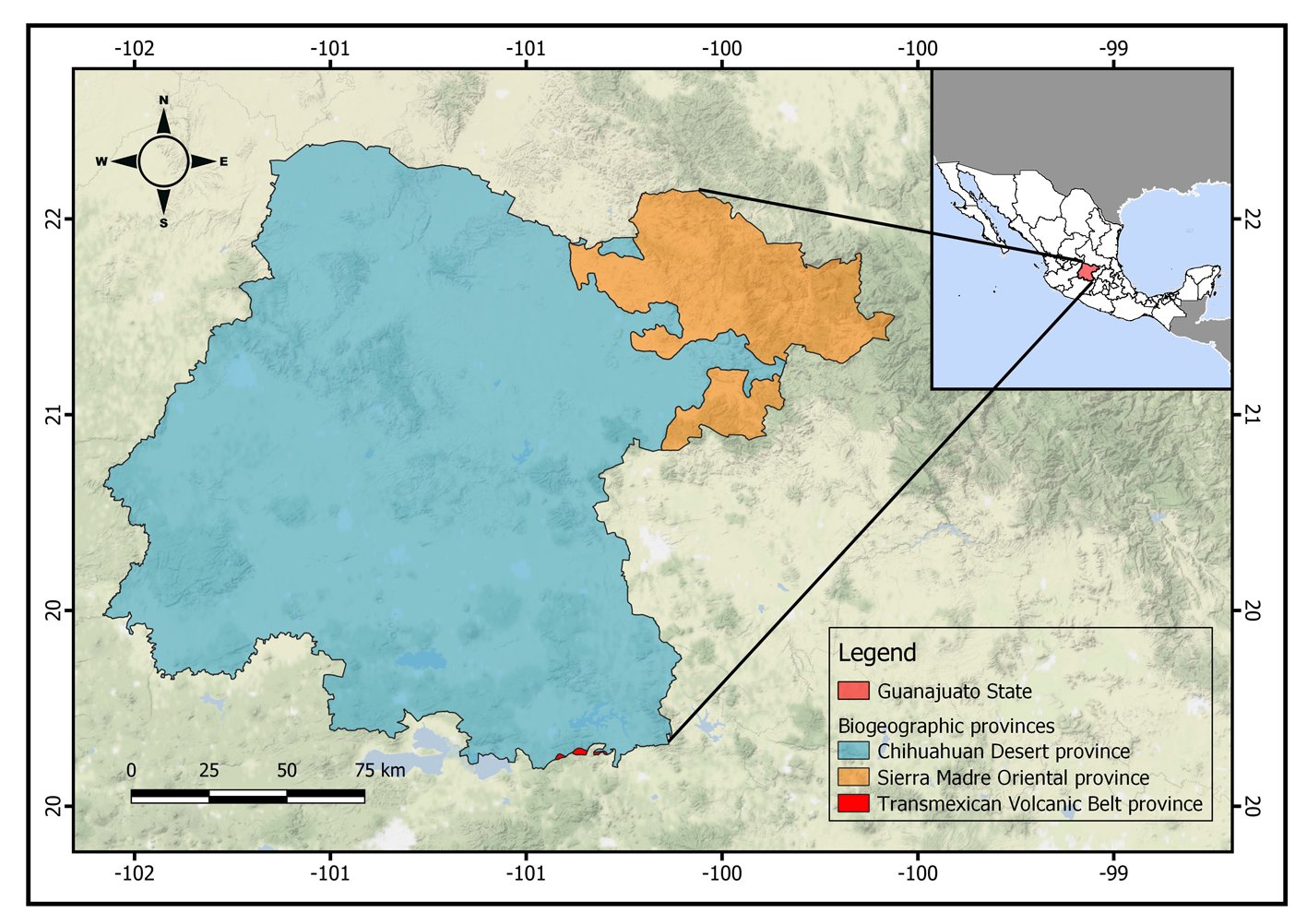
Figure 1. Location of the state of Guanajuato, Mexico, showing the biogeographic provinces.
Amphibians have been recognized as the most threatened terrestrial vertebrate class (Luedtke et al., 2023), and mammals could have significant declination in their populations due to fire, like in Australia (Geary et al., 2023). However, responses of animals to fire could be diverse because they are strongly related to their life-history traits (González et al., 2021). The responses of the amphibian species are variable and incompletely understood (Pilliod et al., 2003); while even among mammalian species, the effect of fire could be not consistent (González et al., 2021). Therefore, the effect of wildfires on distributional patterns of these taxa could be different.
In this study, our aim is to analyze the Linnean and Wallacean shortfalls in the context of the first evaluation of wildfire impacts on biodiversity. We use species of amphibians and mammals of Guanajuato, Mexico, as a study model and use the results to propose priority areas for conservation.
Material and methods
The state of Guanajuato is located in central Mexico, at 19°55’- 21°51’ N, 99°40’ – 102°06’ W. Most of the state is in the Chihuahuan Desert province, with a few areas in Sierra Madre Oriental and Transmexican Volcanic Belt provinces (Morrone et al., 2017; Fig. 1). Guajanuato has 24 Protected Natural Areas (PNA) mainly located in the southwest and center of the state. The largest of these areas is a biosphere reserve (Sierra Gorda), and the other PNA have a range of different levels of protection and activities allowed (SMAOT, 2022).
Although Guanajuato is not among the most biodiverse states in Mexico, it harbors a wide variety of ecosystems, from Pinus and Quercus forests to xerophytic scrubs (Conabio, 2012). Unfortunately, the extent of the agricultural and livestock areas, the high population density, the expansion of urban areas, and industrial activities have contributed to the destruction and disappearance of the original vegetation (Conabio, 2012).
Guanajuato harbors a total of 27 reported species of amphibians and 93 species of mammals, 8 and 25 of which, respectively, have been described as conservation priorities (DOF, 2010; Leyte-Manrique et al., 2022; Sánchez et al., 2016). Of all the species of amphibians and mammals inhabiting Guanajuato, we chose 22 species of amphibians and 13 species of mammals (Table 1) based on the following criteria: 1) valid nomenclature and at least one point record located in Guanajuato in the consulted databases (Flores-Villela & Ochoa-Ochoa, 2020; Escalante et al., 2018; GBIF.org, 2020a-ah); 2) geographic distribution mostly contained within Mexico; 3) at least 25 point records throughout the whole distribution in order to generate reliable species distribution models (SDM); and 4) considered conservation priorities.
In order to evaluate the Linnean and Wallacean shortfalls for those species, we searched the aforementioned databases for all valid point records in Guanajuato. These were initially overlapped to a grid of 0.25º latitude × 0.25º longitude, in QGIS v.3.16.16 (QGIS Development Team, 2020), which will be referred to hereafter as the “state scale”. We built a presence-absence matrix using the generated SDM.
To evaluate the Linnean shortfall based on point records, we quantified the observed richness (Sobs) as the recorded number of species of amphibians and mammals in each quadrat of 0.25º based on locality records. Then, we used the non-parametric estimator Chao2 in R (Kindt & Coe, 2005), to estimate the asymptotic richness of the incidence dataset (Gotelli & Colwell, 2011). The estimated richness Sest in Chao2 was obtained by the formula (Colwell & Coddington, 1994): Sest = Sobs + L2/(2M), where L = number of species that occur in only 1 quadrat, and M = number of species that occur in exactly 2 quadrats. Thus, this calculation provided a measure of how well the richness of each taxonomic group is known for those areas. We also performed the same analysis based on the species distribution models to explore how well the Linnean shortfall was corrected.
Table 1
List of species of amphibians and mammals in Guanajuato, Mexico, and data used in the analyses. Total records = number of point records after the nomenclatural and geographic validation (state scale). Records in Guanajuato = number of point records of each species into the geopolitical boundaries of the state of Guanajuato. Filtered records = subset of point records after the filter of 10 km applied to the total records. Records for modeling = subset of the filtered records used for model training. pROC = ROC partial of the best model.
| Species | Total records | Records in Guanajuato | Filtered records | Records for modeling | pROC |
| Amphibians | |||||
| Ambystoma velasci | 259 | 45 | 247 | 23 | 1.81 |
| Anaxyrus compactilis | 561 | 31 | 488 | 41 | 1.72 |
| Anaxyrus punctatus | 3,798 | 29 | 3,405 | 226 | 1.76 |
| Aquiloeurycea cephalica | 258 | 2 | 227 | 18 | 1.74 |
| Craugastor augusti | 599 | 16 | 508 | 54 | 1.58 |
| Dryophytes arenicolor | 2,514 | 138 | 2,269 | 161 | 1.81 |
| Dryophytes eximius | 820 | 19 | 761 | 72 | 1.75 |
| Eleutherodactylus guttilatus | 136 | 20 | 109 | 12 | 1.79 |
| Eleutherodactylus nitidus | 673 | 5 | 556 | 48 | 1.68 |
| Eleutherodactylus verrucipes | 237 | 2 | 167 | 13 | 1.52 |
| Hypopachus variolosus | 1,323 | 10 | 1,122 | 116 | 1.74 |
| Incilius nebulifer | 5,585 | 13 | 5,200 | 256 | 1.83 |
| Incilius occidentalis | 1,620 | 81 | 1,342 | 114 | 1.71 |
| Isthmura belli | 245 | 1 | 232 | 18 | 1.64 |
| Lithobates berlandieri | 3,747 | 51 | 3,401 | 247 | 1.56 |
| Lithobates megapoda | 127 | 9 | 101 | 12 | 1.65 |
| Lithobates montezumae | 696 | 94 | 598 | 51 | 1.75 |
| Lithobates neovolcanicus | 349 | 51 | 298 | 32 | 1.68 |
| Lithobates spectabilis | 544 | 3 | 416 | 40 | 1.64 |
| Rheohyla miotympanum | 383 | 1 | 329 | 27 | 1.60 |
| Smilisca baudinii | 4,381 | 2 | 3,590 | 277 | 1.68 |
| Spea multiplicata | 2,251 | 38 | 2,008 | 196 | 1.79 |
| Total | 31,090 | 661 | 27,374 | 2,054 | |
| Mammals | |||||
| Choeronycteris mexicana | 578 | 5 | 384 | 72 | 1.71 |
| Corynorhinus mexicanus | 204 | 4 | 149 | 28 | 1.79 |
| Dipodomys ornatus | 85 | 2 | 61 | 12 | 1.78 |
| Table 1. Continued | |||||
| Species | Total records | Records in Guanajuato | Filtered records | Records for modeling | pROC |
| Leptonycteris nivalis | 263 | 1 | 179 | 34 | 1.66 |
| Leptonycteris yerbabuenae | 575 | 9 | 370 | 70 | 1.75 |
| Lepus callotis | 199 | 6 | 150 | 28 | 1.75 |
| Peromyscus melanotis | 601 | 3 | 227 | 42 | 1.84 |
| Peromyscus difficilis | 897 | 10 | 453 | 85 | 1.69 |
| Peromyscus melanophrys | 594 | 25 | 372 | 70 | 1.59 |
| Rhogeessa alleni | 55 | 5 | 46 | 8 | 1.60 |
| Sciurus oculatus | 123 | 34 | 73 | 14 | 1.45 |
| Sigmodon leucotis | 103 | 9 | 72 | 14 | 1.50 |
| Sorex saussurei | 168 | 1 | 93 | 18 | 1.8 |
| Total | 4,445 | 114 | 2,629 | 495 |
To quantify the Wallacean shortfall, we used the Qs estimator (Murguía-Romero & Villaseñor, 2000), which is a measure of the quality of the records. QS can take values between ‘0’ and ‘1’ and is defined as (Murguía-Romero & Villaseñor, 2000): QS = F/[Sobs m/(1 – Es) – max (Sobs, m)], where F = the sum of frequencies of all classes multiplied by all classes (that is, the sum of all ‘1’ in the matrix); Es = measure of the proportion of the known richness related to the estimated richness; and m = the total number of quadrats. Murguía-Romero and Villaseñor (2000) characterized QS values above 80% as “very good”, values between 50% to 80% as “good” and less than 50% as “poor” data quality.
To compare the possible effect of the Wallacean shortfall in the biogeographic patterns, we performed a species distribution model (SDM) for each species in order to obtain a map of richness patterns for amphibians and mammals. Following the BAM diagram of Soberón and Peterson (2005), where the M corresponds to the region that is reachable by the species from established distributional areas in ecological time (Soberón & Peterson, 2005). The M for each species was obtained using the concept of extent of occurrence, defined as “the area contained within the shortest continuous imaginary boundary that can be drawn to encompass all the known, inferred or projected sites of present occurrence of a taxon, excluding cases of vagrancy” (IUCN, 2001). Therefore, we defined M as the area within a minimum convex hull polygon for each species constructed in QGIS v.3.16.16 (QGIS Development Team, 2020).
The M of each species was used to crop the 19 environmental layers of WorldClim 2 (Fick & Hijmans, 2017) and 3 topographic variables (slope, elevation and aspect; USGS, 2021) at ~ 1 km2 of resolution. The data points were filtered in Wallace software (Kass et al., 2018) to a distance of 10 km between points to reduce spatial biases, and retain useful information (Aiello-Lammens et al., 2015; Pearson et al., 2007). To avoid collinearity among the 22 variables for each species, we obtained the VIF (Mandeville, 2008; Montgomery & Peck, 1992), applying the packages usdm (Naimi et al., 2014) and rgdal (Bivand et al., 2015) in RStudio (RStudio Team, 2020).
The models were performed in the maximum entropy package kuenm (Cobos et al., 2019) in RStudio (RStudio Team, 2020). The occurrence dataset for each species was divided as follows: 75% of the points were used for training and 25% for testing; and a set of independent occurrences of 25% for a last evaluation; those datasets were built with the kuenm_occsplit function in kuenm. For the next step, we used the function kuenm_cal, using the feature classes: linear, quadratic and hinge; and the regularization multipliers 0.5, 1, 1.5, 2, 2.5, 3, 3.5 and 4. All models were evaluated with kuenm_ceval, calculating the ROC partial with E = 10 (Peterson et al., 2008), and Akaike criterion for small samples (AICc; Warren & Seifert, 2011). The final best model for each species was obtained on a clog-log scale using the pROC value in NicheToolbox (Osorio-Olvera et al., 2020).
To produce binary maps of geographic distribution area of each species, the final best model was reclassified using the “10th percentile training presence” threshold, and cropped to the political boundaries of Guanajuato.
Wildfires. We used hotspot data from the MODIS sensor at a resolution of 1 km2 for the years 2000 to 2021, downloaded from NASA Earth Data Cloud (2020). Each hotspot was overlapped to a net of ~ 1 km2 covering the state of Guanajuato in QGIS (QGIS Development Team, 2020), and we counted the number of hotspots in each square of the net. This area will be referred to as the “fine scale”.
In order to compare the number of fires in each square of the net with the scale of the models, we transformed this number between ‘0’ and ‘1’ through a min-max normalization (Farrús et al., 2007; Jain et al., 2005). This procedure was useful to evaluate the effect of the wildfires on the SDM of each species. All cartographic products were projected to UTM zone 14 north coordinates, which corresponds to the state of Guanajuato. To quantify the impact of the fires on species richness patterns, we rasterized the map of the number of fires, from which we produced a new map of kernel density with a radius of 3,000 m, using the software DINAMICA EGO (Ferreira et al., 2019). The map of kernel density was multiplied by the richness map for each taxonomic group. Finally, we quantified the burned area for the maps and for the Protected Natural Areas (SMAOT, 2022).
Results
Shortfalls. We obtained 31,090 records of amphibians considering the whole distribution for the 22 amphibian species, and 661 records within Guanajuato. For the 13 species of mammals, the number of records was 74 in Guanajuato and 2,629 in the whole distribution. The species with the most records was the coastal plain toad Incilius nebulifer (5,585 records) for the amphibians and the southern rock mouse Peromyscus difficilis (453 records; see Table 1) for the mammals. However, within Guanajuato, there were only 13 and 9 records for these species, respectively. The species with the highest number of point records within Guanajuato were the canyon tree frog Dryophytes arenicolor with 138 records, and the Peters’s squirrel Sciurus oculatus, with 34 records.
The richest 0.25º quadrat for amphibians had 11 species and the quadrat with the most mammals had 5 species, while the lowest number of species per quadrat was 1 for both taxa, although there were a few marginal quadrats without data for amphibians and some complete quadrats without data for mammals (~ 12). The maps of quadrats with the observed richness (Sobs in Chao2) for both groups are shown in the Supplementary material: figures 1S, 2S. The main results of the Chao2 estimator are shown in Table 2. For both groups, the number of observed species (Sobs) was lower than the expected number (Sest) for Guanajuato. In the case of the Chao2 estimated with species distribution models, the species richness was the same as the expected species.
Regarding the Wallacean shortfall, the Qs estimator had a value of 23% for the amphibians and 28% for mammals at the state scale. These values were categorized as “poor” quality data in both taxa, but Qs was worse in amphibians.
Table 2
Results of the recorded and estimated richness for the complete distributional data of amphibians and mammals of Guanajuato, Mexico based both on species richness and on species distribution models (SDM).
| Taxonomic group | Recorded richness (Sobs) | Estimated richness (Sest) | Standard deviation (SD) | Estimated richness with SDM (Sest) |
| Amphibians | 22 | 24.61 | 3.42 | 24 |
| Mammals | 13 | 14.94 | 3.64 | 14 |

Figure 2. Richness pattern for 22 modeled species of amphibians and the Protected Natural Areas in Guanajuato, Mexico (black polygons): 1. Palenque, 2. Peña Alta, 3. Sierra de Pénjamo, 4. Sierra de los Agustinos, 5. Las Fuentes, 6. Sierra de Lobos, 7. Las Musas, 8. Lago Cráter La Joya, 9. Cerro de los Amoles, 10. Parque Metropolitano, 11. Cerro de Arandas, 12. Cuenca Alta del Río Temascatio, 13. Cerro del Cubilete, 14. Cerros El Culiacán y La Gavia, 15. Cuenca de La Esperanza, 16. Mega Parque de la Ciudad de Dolores Hidalgo, 17. Presa La Purísima y su Zona de Influencia, 18. Presa de Neutla y su Zona de Influencia, 19. Laguna de Yuriria y su Zona de Influencia, 20. Pinal de Zamorano, 21. Región Volcánica Siete Luminarias, 22. Sierra Gorda de Guanajuato, 23. Cuenca de la Soledad, 24. Presa de Silva y Áreas Aledañas.
Some results of the modeling process are shown in Table 1. The distribution models of amphibians predicted that the species Craugastor augusti, Dryophytes arenicolor, Dryophytes eximius, Incilius occidentalis, Lithobates montezumae, Lithobates neovolcanicus, and Spea multiplicata are distributed in more than 90% of the surface of Guanajuato. Meanwhile, the species Aquiloeurycea cephalica (31%), Smilisca baudini (25%), Lithobates berlandieri (19%), and Incilius nebulifer (3%) had the lowest proportion of distribution in Guanajuato. Regarding the mammals, Choeronycteris mexicana, Corynorhynus mexicanus, Leptonycteris nivalis, Lepus callotis, Peromyscus difficilis, Peromyscus melanophrys, and Peromyscus melanotis were the most widely distributed in Guanajuato (more than the 90% of the state is predicted as part of their distribution), while Sorex saussurei was the only species with a proportion less than 30%.
For the richness patterns, the pixels with highest number of species modeled to be present were similar between amphibians and mammals at the fine scale (Figs. 2, 3), showing a diagonal strip of high richness from the northwest to the southeast, which coincided with 14 PNA: Las Fuentes, Sierra de Lobos, Parque Metropolitano, Cuenca Alta del Río Temascatío, Cerro del Cubilete, Cuenca de La Esperanza, Presa de Neutla, Cuenca de la Soledad, Sierra de los Agustinos, Lago Cráter La Joya, Cerro de los Amoles, Cerros El Culiacán y La Gavia, Laguna de Yuriria and Región Volcánica Siete Luminarias. There were also other sites of high diversity, for example within the PNA of Sierra de Pénjamo and Sierra Gorda.
Wildfires. The maximum number of wildfires per quadrant at the fine scale was 6. To further explore the risk of wildfire recurrence, we built a risk map using the recurrence of fires in each square, with 3 classes: 1) low risk, for pixels with one fire during the analyzed period; 2) medium risk, for pixels with 2 or 3 fires; and 3) high risk, for pixels with 4, 5 or 6 fires (Fig. 4). A large proportion of quadrats with high recurrence of fires occurred outside PNA (for example at northern Guanajuato), but there were also some high risk zones within PNA, like Palenque, Peña Alta, Sierra de Pénjamo, Las Musas and Región Volcánica Siete Luminarias.

Figure 3. Richness pattern for 13 modeled species of mammals and the Protected Natural Areas in Guanajuato, Mexico (black polygons): 1. Palenque, 2. Peña Alta, 3. Sierra de Pénjamo, 4. Sierra de los Agustinos, 5. Las Fuentes, 6. Sierra de Lobos, 7. Las Musas, 8. Lago Cráter La Joya, 9. Cerro de los Amoles, 10. Parque Metropolitano, 11. Cerro de Arandas, 12. Cuenca Alta del Río Temascatio, 13. Cerro del Cubilete, 14. Cerros El Culiacán y La Gavia, 15. Cuenca de La Esperanza, 16. Mega Parque de la Ciudad de Dolores Hidalgo, 17. Presa La Purísima y su Zona de Influencia, 18. Presa de Neutla y su Zona de Influencia, 19. Laguna de Yuriria y su Zona de Influencia, 20. Pinal de Zamorano, 21. Región Volcánica Siete Luminarias, 22. Sierra Gorda de Guanajuato, 23. Cuenca de la Soledad, 24. Presa de Silva y Áreas Aledañas.
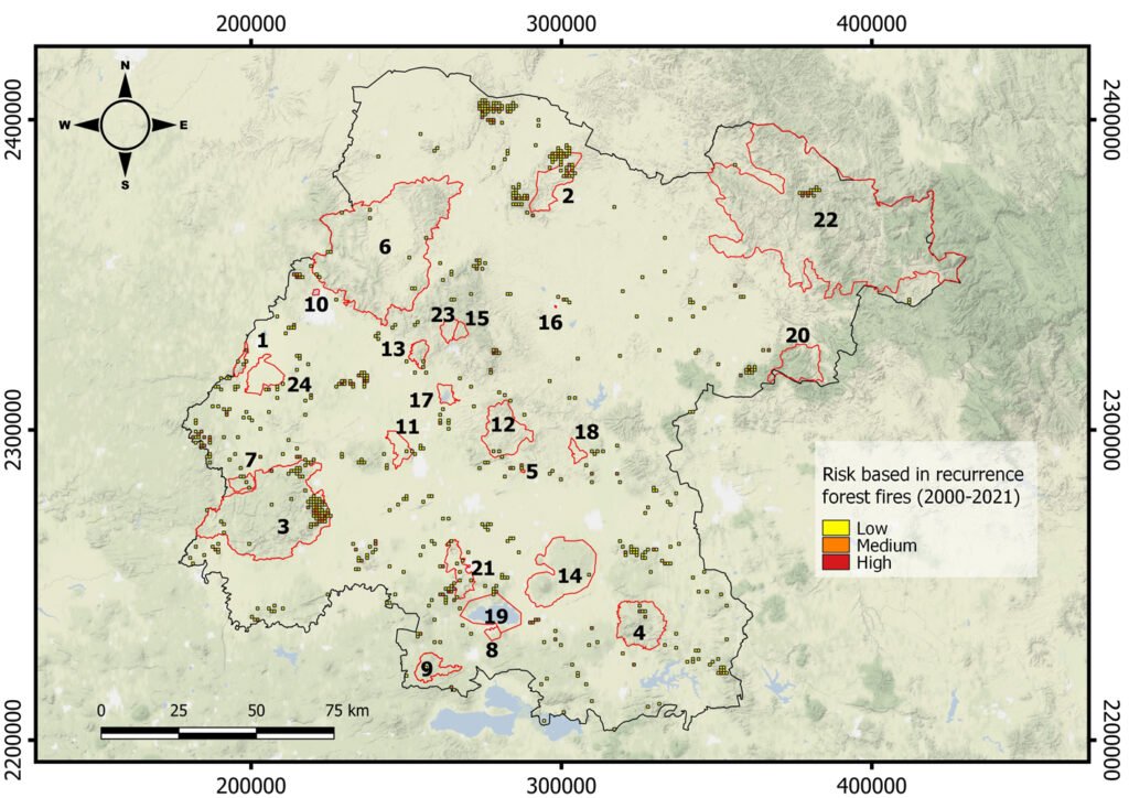
Figure 4. Map of fire risk in Guanajuato between the years 2000 and 2021, based on the recurrence of fires in a 1 km square, with 3 classes: (1) low risk, for squares with one fire during the analyzed period; (2) medium risk, for squares with 2 or 3 fires; and (3) high risk, for squares with 4, 5 or 6 fires. Red polygons represent the Protected Natural Areas.
Table 3
Potential distribution area predicted by the modeling for 22 amphibian and 13 mammal species and quantification of habitat lost due to wildfires relative to the total area of Guanajuato, Mexico (30,702 km2).
| Species | Surface of potential distribution area occupied in Guanajuato (km2) | Percentage of potential distribution area occupied (%) | Surface of potential distribution area affected by wildfires (km2) | Percentage of potential distribution area affected by wildfires (%) |
| Amphibians | ||||
| Ambystoma velasci | 22,351 | 73 | 3,620 | 16 |
| Anaxyrus compactilis | 26,061 | 85 | 4,948 | 19 |
| Anaxyrus punctatus | 18,241 | 59 | 2,440 | 13.3 |
| Aquiloeurycea cephalica | 9,653 | 31 | 1,246 | 12.9 |
| Craugastor augusti | 30,702 | 100 | 5,264 | 17.1 |
| Dryophytes arenicolor | 30,696 | 99.9 | 5,262 | 17.1 |
| Dryophytes eximius | 30,267 | 98.5 | 5,249 | 17.3 |
| Eleutherodactylus guttilatus | 21,636 | 70 | 2,088 | 14.2 |
| Eleutherodactylus nitidus | 22,888 | 75 | 4,663 | 20.3 |
| Eleutherodactylus verrucipes | 20,519 | 67 | 2,756 | 13.4 |
| Hypopachus variolosus | 19,076 | 62 | 3,951 | 20.7 |
| Incilius nebulifer | 873 | 3 | 55 | 6.3 |
| Incilius occidentalis | 30,546 | 99 | 5,257 | 17.2 |
| Isthmura bellii | 26,647 | 87 | 4,925 | 18.4 |
| Lithobates berlandieri | 5,772 | 19 | 614 | 10.6 |
| Lithobates megapoda | 20,866 | 68 | 4,422 | 21.1 |
| Lithobates montezumae | 29,957 | 97.5 | 5,242 | 17.4 |
| Lithobates neovolcanicus | 28,670 | 93 | 5,137 | 17.9 |
| Lithobates spectabilis | 24,821 | 81 | 3,893 | 15.6 |
| Rheohyla miotympanum | 18,056 | 59 | 3,516 | 19.4 |
| Smilisca baudinii | 7,631 | 25 | 1,579 | 20.6 |
| Spea multiplicata | 30,661 | 99.8 | 5,264 | 17.1 |
| Mammals | ||||
| Choeronycteris mexicana | 30,608 | 99.69 | 5,242 | 17.12 |
| Corynorhynus mexicanus | 30,608 | 99.69 | 5,242 | 17.12 |
| Dipodomys ornatus | 18,553 | 60.43 | 3,429 | 18.48 |
| Leptonycteris nivalis | 30,608 | 99.69 | 5,242 | 17.12 |
| Leptonycteris yerbabuenae | 24,955 | 81.28 | 4,474 | 17.93 |
| Lepus callotis | 28,469 | 92.73 | 5,025 | 17.65 |
| Peromyscus difficilis | 30,142 | 98.18 | 5,225 | 17.34 |
| Peromyscus melanophrys | 29,606 | 96.43 | 5,227 | 17.65 |
| Peromyscus melanotis | 29,231 | 95.21 | 5,183 | 17.73 |
| Rhogessa alleni | 17,604 | 57.34 | 3,353 | 19.05 |
| Sciurus oculatus | 14,564 | 47.44 | 1,923 | 13.20 |
| Sigmodon leucotis | 18,215 | 59.33 | 3,139 | 17.23 |
| Sorex saussurei | 4,151 | 13.52 | 756 | 18.22 |

Figure 5. Richness map of amphibians intersected with the kernel density of recurrence of the wildfires in Guanajuato, Mexico. Black polygons represent the Protected Natural Areas.
1. Palenque, 2. Peña Alta, 3. Sierra de Pénjamo, 4. Sierra de los Agustinos, 5. Las Fuentes, 6. Sierra de Lobos, 7. Las Musas, 8. Lago Cráter La Joya, 9. Cerro de los Amoles, 10. Parque Metropolitano, 11. Cerro de Arandas, 12. Cuenca Alta del Río Temascatio, 13. Cerro del Cubilete, 14. Cerros El Culiacán y La Gavia, 15. Cuenca de La Esperanza, 16. Mega Parque de la Ciudad de Dolores Hidalgo, 17. Presa La Purísima y su Zona de Influencia, 18. Presa de Neutla y su Zona de Influencia, 19. Laguna de Yuriria y su Zona de Influencia, 20. Pinal de Zamorano, 21. Región Volcánica Siete Luminarias, 22. Sierra Gorda de Guanajuato, 23. Cuenca de la Soledad, 24. Presa de Silva y Áreas Aledañas.
Respect to the temporal distribution of the recurrence of forest fires, for the period of time analyzed, the years 2017, 2019, and 2021 had the highest number of fires (72, 110 and 150, respectively). The map of kernel density is shown in Supplementary material: Figure 3S. The map was transformed to a binary map and overlapped with the patterns of richness of amphibians and mammals, to produce the maps in figures 5, 6.
The evaluation of the effects of the wildfires on the model of each species is shown in Table 3. The mean percentage of burned potential distribution area was 16.49 and 17.37 for amphibians and mammals, respectively. Some species’ distribution areas were more strongly affected by fires, such as Eleutherodactylus nitidus, Hypopachus variolosus, Lithobates megapode, and Smilisca baudinii, all of which were amphibians for which more than 20% of their distribution area had been burned. For mammals, the most affected species was Rhogessa alleni (19.05%), followed by Sorex saussurei (18.22%).
The area of Guanajuato affected by fires measured nearly 5,200 km2 (17%; Figs. 5, 6), with high diversity zones for amphibians located in the northwest, near Sierra de Lobos (PNA 6) and Peña Alta (PNA 2). Other important affected areas for amphibians coincided with high recurrence of wildfires in the southern of Guanajuato in Región Volcánica Siete Luminarias (PNA 21), Sierra de los Agustinos (PNA 4) and Cerro de los Amoles (PNA 9). For mammals, some of the most strongly affected areas coincided with those of the amphibians (e.g., within Cerro de los Amoles; PNA 9), but there were also areas that were unique to mammals (Fig. 6). For example, there were areas of high mammal richness with wildfires in central Guanajuato, which did not coincide with any PNA, as well as southeastern areas in Sierra de los Agustinos (PNA 4). Fortunately, areas with high richness for both amphibians and mammals were not affected by fires, like Sierra de Lobos (PNA 6), Cuenca de la Esperanza (PNA 15), and Cuenca de la Soledad (PNA 23).
Discussion
Linnean shortfalls in the state of Guanajuato could have medium effects because the estimator predicted at least 2 additional species for each taxon relative to total currently known. This suggests that the current species inventories are not yet complete. This finding does not dismiss possible shortfalls at more detailed scales, because the number of records within the state of Guanajuato is very low, with an average of 30 per each species of amphibian and only 6 of each species of mammal. It would therefore be informative to carry out more specific analyses within the quadrats where 0 or 1 species were recorded. Increased collection effort in the field could improve the problems of undersampling, since the number of total data points in Guanajuato is very low for some species (v. gr. Aquiloeurycea cephalica with 2 records, and Leptonycteris nivalis with 1 record; Table 1). It is interesting to highlight that when performing the analyses with SDM, the Linnean shortfall is apparently corrected (Table 2). However, these results should be taken with caution, because it is possible that there are commission errors in models or that those areas actually correspond to sister species (Rodrigues et al., 2019; Acevedo et al., 2014).
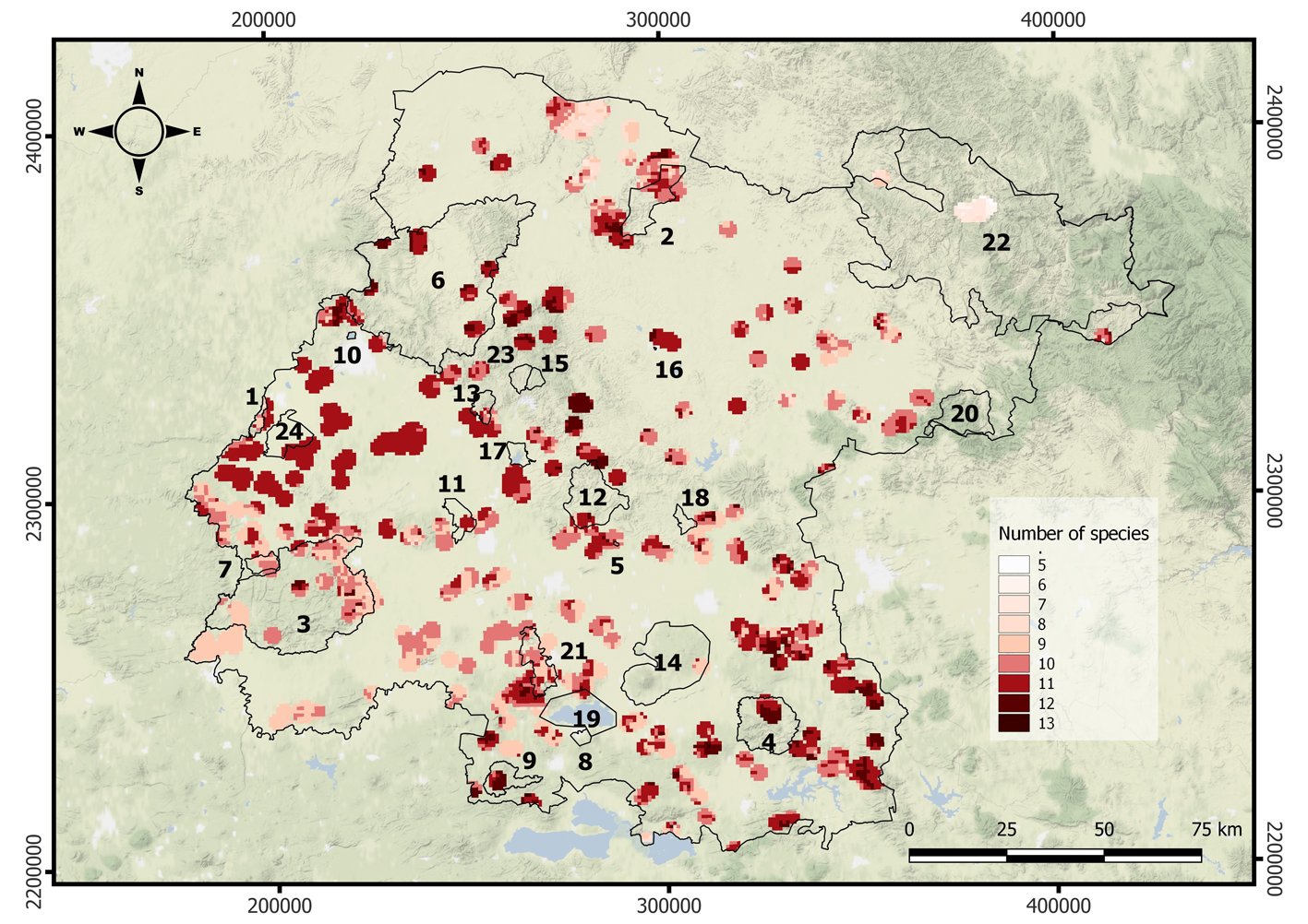
Figure 6. Richness map of mammals intersected with the kernel density of recurrence of the wildfires in Guanajuato, Mexico. Black polygons represent the Protected Natural Areas.
1. Palenque, 2. Peña Alta, 3. Sierra de Pénjamo, 4. Sierra de los Agustinos, 5. Las Fuentes , 6. Sierra de Lobos, 7. Las Musas, 8. Lago Cráter La Joya, 9. Cerro de los Amoles, 10. Parque Metropolitano, 11. Cerro de Arandas, 12. Cuenca Alta del Río Temascatio, 13. Cerro del Cubilete, 14. Cerros El Culiacán y La Gavia, 15. Cuenca de La Esperanza, 16. Mega Parque de la Ciudad de Dolores Hidalgo, 17. Presa La Purísima y su Zona de Influencia, 18. Presa de Neutla y su Zona de Influencia, 19. Laguna de Yuriria y su Zona de Influencia, 20. Pinal de Zamorano, 21. Región Volcánica Siete Luminarias, 22. Sierra Gorda de Guanajuato, 23. Cuenca de la Soledad, 24. Presa de Silva y Áreas Aledañas.
On the other hand, the Wallacean shortfall was highly relevant for both amphibians and mammals, showing poor quality. Murguía-Romero and Villaseñor (2000) suggested that the quality of the records is related to the geographical resolution of the biogeographical analysis. In future analysis within the state of Guanajuato and using smaller quadrats (for example, close in size to the pixels of our models), the Wallacean shortfall could strongly affect the observed data, reaching very poor data quality. Thus, it seems to be the more important shortfall for these vertebrate species.
For our 25 species, probably the effect of the Linnean shortfall has a less dramatic effect than the Wallacean shortfall. There are multiple potential explanations for these shortfalls, including low intensity and spatial variation of sampling, which can directly affect biodiversity estimators like species richness (Oliveira et al., 2016). Continuing the study of these shortfall will be important for the correct implementation of conservation strategies, for example with other methods including correlations using the sampling effort (Oliveira et al., 2016), rate of descriptions and number of taxonomists (Joppa et al., 2011), many different algorithms of species distribution modeling and maps of ignorance (Oliveira et al., 2016; Rocchini et al., 2011; Tessarolo et al., 2021), among others.
In spite of the extant Wallacean shortfalls, the richness patterns for both taxa were partially recognized; specially, the recorded most richness quadrats at 0.25º also showed the modeled pattern for amphibians. For mammals, the highest richness area near to Cuenca de la Esperanza was identified also for a quadrat of 0.25º, coinciding with the models. Amphibians and mammals shared many (though not all) areas of high richness, generally following a northwest-southeast diagonal across the state. The partial similarity in those richness patterns could be useful in Systematic Conservation Planning, because both taxa could represent each other as good surrogates (Escalante et al., 2020).
In general, amphibians and mammals are over-represented taxa in databases, although amphibians are less represented than mammals (Troudet et al., 2017). Few articles have quantified the Linnean and Wallacean shortfalls prior to biogeographic analysis. In particular, Oliveira et al.(2016) suggested that terrestrial vertebrates have similar biases compared with some taxa of arthropods, contradicting the statement that terrestrial vertebrates are better suited for biogeographic and conservation studies. In some places, such as the state of Guanajuato, amphibians and mammals could have similar Linnean shortfalls, but differ in the severity of their Wallacean shortfalls, which could modify the biogeographic patterns identified.
The relevance of including shortfall analysis in biogeographical studies, mainly in those related to species conservation, lies in the fact that the Linnean and Wallacean shortfalls strongly influence the possible results, since the data on the identity and distribution of the species are crucial to identify patterns in biodiversity, as well as the processes that modify those patterns (Hortal et al., 2015). In particular, Wallacean shortfalls can also alter estimates of threatened conservation status, since range size is regularly used in conservation (Hortal et al., 2015). Species with small ranges have higher priority in many international and national standards (DOF, 2010; IUCN, 2012). Therefore, Wallacean shortfalls could lead to some taxa and areas being disproportionately prioritized over others because their distribution areas have been erroneously underestimated (Riddle et al., 2011). In addition, other shortfalls that potentially can affect the biogeographic patterns should be investigated, like Darwinian shortfall (Diniz-Filho et al., 2013, 2023), and even distinct categories of Linnean shortfalls (Vergara-Asenjo et al., 2023).
As we expected, wildfires affected all species, but in different ways. For amphibians, the species Smilisca baudinii, in addition to having a small distribution area in Guanajuato compared to the rest of the species, is one of the most affected by wildfires occurrences. These observations may suggest that Smilisca baudinii should be considered a priority species for conservation in the state of Guanajuato. Furthermore, we also highlight Lithobates megapoda, which is listed in the 2019 update of the NOM-059-SEMARNAT-2010 (DOF, 2019) as a species under special protection and described as sensitive to habitat degradation (Santos-Barrera & Flores-Villela, 2004).
On the other hand, in the northeastern part of the state, the effects seem to be minimal compared to the south and southwest, but it is important to remember that species with specific habitat requirements such as Incilius nebulifer, Lithobates berlandieri, and Smilisca baudinii are distributed in this area. Therefore, attention should be paid to investigating the sources of ignition present at this area in order to prevent future wildfires, since the loss of habitat could result in the disappearance of these species. Finally, in accordance with Clivillé et al.(1997), who describe the effect of fires on amphibians from 3 points of view (habitat, species and individual), our study only focuses on the effect of these events on the habitat. Thus, the effects on the distribution of the selected species can be interpreted as loss of habitat and vegetation cover, trophic resources and humidity due to wildfires, which are determining characteristics for the presence of amphibians and their reproduction (Clivillé et al., 1997).
For the case of mammals, Sorex saussurei (the Saussure’s shrew) is the species with the narrowest geographic distribution in Guanajuato. This shrew is only distributed in Mexico and Guatemala, and even though it is considered as least concern on the Red List of Threatened Species (IUCN, 2017), some populations in Mexico have been categorized as threatened and under special protection (DOF, 2019). Secondly, Peters’s squirrel Sciurus oculatus occupies less than 50% of the surface of Guanajuato and is also categorized as least concern in the Red List of Threatened Species (IUCN, 2016). Sciurus oculatus is found only within Mexico, and is under special protection in national legislation NOM-059-SEMARNAT-2010, update of 2019 (DOF, 2019). Both species face continuing decline in the extent and quality of habitat due to land use change (Conafor, 2020; IUCN, 2016, 2017), which is exacerbated by repeated burning episodes that decrease the area occupied by each species by 13-18%. According to Zamudio (2012), most of the plant communities in the state of Guanajuato have significantly changed in their structure, floristic composition and physiognomy. Consequently, their distribution areas have been gradually reduced. Currently, 63% of the territory has been transformed into agricultural areas, human settlements, and areas devoid of vegetation (Roth et al., 2016).
The recurrence of wildfires, mainly in the southern part of Guanajuato, represents an important threat to biodiversity conservation within PNA, which are surrounded by a complex matrix of rainfed and irrigated agricultural land uses. This result was also found by Farfán et al. (2020, 2021), where both the probabilities of anthropogenic ignition and climate under the ENSO climate conditions lead to high wildfire risk in this region of the state. These PNA urgently need fire management plans that can integrate fire prevention actions at the local level in the context of global warming. On a global scale, wildfires have been responsible for up to 27% of the loss of tree cover between 2001 and 2021 (Tyukavina et al., 2022). In Mexico alone, in 2021, 408.75 km2 of forest were lost due to fire (Tyukavina et al., 2022). The effects of wildfires on biodiversity patterns could be understimated if these shortfalls are underestimating the biodiversity. Therefore, actions at the international level are also urgent in order to prevent damage to unknown biogeographic patterns.
This is the first study for the state of Guanajuato and for Mexico that addresses the effect of wildfire on the potential distribution of 2 important taxonomic groups: amphibians and mammals. The evaluation of the Linnean and Wallacean shortfalls for any taxonomic group is essential before the identification of geographic patterns involved as criteria for conservation planning, even in terrestrial vertebrates which are assumed to be adequately sampled. The Wallacean shortfall could lead to underestimations of the effects of perturbations such as wildfires. This is particularly true of species that are already vulnerable due to anthropogenic factors such as land cover change, illegal trafficking, etc., as well as intrinsic factors like the size of their natural distributional areas, because it is unknown whether undersampling could represent geographically rare species. Improving the biogeographical knowledge of the patterns of amphibians and mammals could provide better tools to stakeholders in order to generate fire management plans to prevent the negative impact of the wildfire within protected areas around the world.
Acknowledgements
We thank Julián A. Velasco and Luis J. Aguirre for their help with the parametrization of Maxent, and Miguel Murgía for assistance with the quantification of the Qs estimator. We also thank to the anonymous reviewers and the Associate Editor for their careful reading of this manuscript.
References
Acevedo, P., Melo-Ferreira, J., Real, R., & Alves, P. C. (2014). Evidence for niche similarities in the allopatric sister species Lepus castroviejoi and Lepus corsicanus. Journal
of Biogeography, 41, 977–986. https://doi.org/10.1111/jbi.12
270
Aiello-Lammens, M. E., Boria, R. A., Radosavljevic, A., Vilela, B., & Anderson, R. P. (2015). spThin: an R package for spatial thinning of species occurrence records for use in ecological niche models. Ecography, 38,541–545. https://doi.org/10.1111/ecog.01132
Barlow, J., Berenguer, E., Carmenta, R. & França, F. (2020). Clarifying Amazonia’s burning crisis. Global Change Biology, 26, 319–321. https://doi.org/10.1111/gcb.14872op
Bivand, R., Keitt, T., Rowlingson, B., Pebesma, E., Sumner, M., Hijmans, R. et al. (2015). Package ‘rgdal’. Bindings for the Geospatial Data Abstraction Library. Retrieved on December, 2020 from: http://rgdal.r-forge.r-project.org
Chisholm, R. A., Wijedasa, L. S., & Swinfield, T. (2016). The need for long-term remedies for Indonesia’s forest fires. Conservation Biology, 30, 5–6. https://doi.org/10.1111/cobi.
12662
Chuvieco, E., Giglio, L. & Justice, C. (2008). Global characterization of fire activity: toward defining fire regimes from Earth observation data. Global Change Biology, 14, 1488–1502. https://doi.org/10.1111/j.1365-2486.2008.01585.x
Clivillé, S., Montori, A., Llorente, G. A., Santos, X., & Carretero, M. A. (1997). El impacto de los incendios forestales sobre los anfibios. Quercus, 138,10–13.
Cobos, M. E., Peterson, A. T., Barve, N., & Osorio-Olvera, L. (2019). Kuenm: An R package for detailed development of ecological niche models using Maxent. PeerJ, 7,e6281. https://doi.org/10.7717/peerj.6281
Colwell, R. K., & Coddington, J. A. (1994). Estimating terrestrial biodiversity through extrapolation. Philosophical Transactions of the Royal Society B, 345, 101–118. https://doi.org/10.1098/rstb.1994.0091
Conabio (Comisión Nacional para el Conocimiento y Uso de la Biodiversidad). (2012). La biodiversidad en Guanajuato: estudio de estado (Vol. II). Guanajuato, Mexico: Comisión Nacional para el Conocimiento y Uso de la Biodiversidad (Conabio)/ Instituto de Ecología del Estado de Guanajuato (IEE).
Conafor (Comisión Nacional Forestal). (2020). Estimación de la tasa de deforestación bruta en México para el periodo 2001-2018 mediante el método muestreo. Documento técnico. Comisión Nacional Forestal. Jalisco, México. Retrieved in 2022 from: http://www.conafor.gob.mx:8080/documentos/docs/1/7768Documento%20tecnico%202020%20Deforestacion%20Bruta%20Final.pdf
DOF (Diario Oficial de la Federación). (2010). NORMA
Oficial Mexicana NOM-059-SEMARNAT-2010, Protección ambiental-Especies nativas de México de flora y fauna silvestres-Categorías de riesgo y especificaciones para
su inclusión, exclusión o cambio-Lista de especies en
riesgo. Mexico City, Mexico. Retrieved on March 3rd, 2021 from: https://dof.gob.mx/nota_detalle_popup.php?
codigo=5173091
DOF (Diario Oficial de la Federación). (2019). Modificación del Anexo Normativo III, Lista de especies en riesgo de la Norma Oficial Mexicana NOM-059-SEMARNAT-2010, Protección ambiental-Especies nativas de México de flora y fauna silvestres-Categorías de riesgo y especificaciones para su inclusión, exclusión o cambio-Lista de especies en riesgo, publicada el 30 de diciembre de 2010. Secretaría de Gobernación (SEGOB). Mexico City, Mexico. Retrieved on March 03rd, 2021 from: https://www.dof.gob.mx/nota_detalle.php?codigo=5578808&fecha=14/11/2019#gsc.tab=0
Diniz-Filho, J. F, Jardim, L., Guedes, J. J., Meyer, L., Stropp, J., Frateles, L. E. et al. (2023). Macroecological links between the Linnean, Wallacean, and Darwinian shortfalls. Frontiers of Biogeography, 15, e59566. http://dx.doi.org/10.21425/F5FBG59566
Diniz-Filho, J. A. F., Loyola, R. D., Raia, P., Mooers, A. O., & Bini, L. M. (2013) Darwinian shortfalls in biodiversity conservation. Trends in Ecology and Evolution, 28, 689–695. https://doi.org/10.1016/j.tree.2013.09.003
Escalante, T., Noguera-Urbano, E. A., & Corona, W. (2018). Track analysis of the Nearctic region: Identifying complex areas with mammals. Journal of Zoological Systematics and Evolutionary Research, 56, 466–477. https://doi.org/10.1111/jzs.12211
Escalante, T., Varela-Anaya, A. M., Noguera-Urbano, E. A., Elguea-Manrique, L. M., Ochoa-Ochoa, L. M., Gutiérrez-Velázquez, A. L. et al. (2020). Evaluation of five taxa as surrogates for conservation prioritization in the Trans-
mexican Volcanic Belt, México. Journal for Nature Conservation, 54, e125800. https://doi.org/10.1016/j.jnc.20
20.125800
Farfán, M., Pérez-Salicrup, D. R., Flamenco-Sandoval, A., Nicasio-Arzeta, S., Mas, J. F., & Ramírez-Ramírez, I. (2018). Modeling anthropic factors as drivers of wildfire occurrence at the Monarch Butterfly Biosphere. Madera y Bosques, 24, 1–15. https://doi.org/10.21829/myb.2018.2431591
Farfán, M., Flamenco-Sandoval, A., Rodríguez-Padilla, C. R., Rodrigues-de Sousa Santos, L., González-Gutiérrez, I., & Gao, Y. (2020). Cartografía de la probabilidad de ocurrencia a incendios forestales para el estado de Guanajuato: Una aproximación antrópica de sus fuentes de ignición. Acta Universitaria, 30, 1–15. https://doi.org/10.15174/au.2020.2953
Farfán, M., Domínguez, C., Espinoza, A., Jaramillo, A., Alcántara, C., Maldonado, V. et al. (2021). Forest fire probability under ENSO conditions in a semi-arid region: a case study in Guanajuato. Environmental Monitoring and Assessment, 193, 1–14. https://doi.org/10.1007/s10661-021-09494-0
Farrús, M., Anguita, J., Hernando, J., & Cerdà, R. (2007). Fusión de sistemas de reconocimiento basados en características de alto y bajo nivel. In III Congreso da Sociedade Española de Acústica Forense: actas do Congreso; 2005 oct 27-28; Santiago de Compostela, España. Santiago de Compostela: Dirección Xeral de Creación e Difusión Cultural.
Ferreira, B. M., Soares-Filho, B. S., & Quintão, F. M. (2019). The Dinamica EGO virtual machine. Science of Computer Programming, 173,3–20. https://doi.org/10.1016/j.scico.20
18.02.002
Fick, S. E., & Hijmans, R. J. (2017). WorldClim 2: new 1-km spatial resolution climate surfaces for global land areas. International Journal of Climatology, 37,4302–4315. https://doi.org/10.1002/joc.5086
Flores-Villela, O., & Ochoa-Ochoa, L. M. (2020). Compilación de bases de datos de la herpetofauna mexicana. Museo de Zoología “Alfonso L. Herrera”, Facultad de Ciencias, Universidad Nacional Autónoma de México. Ciudad de México.
GBIF.org. (2020a). GBIF Occurrence Download. Retrieved on November 11th, 2020 from: https://doi.org/10.15468/dl.
bbt2tq
GBIF.org. (2020b). GBIF Occurrence Download. Retrieved on November 11th, 2020 from: https://doi.org/10.15468/dl.
j9evdt
GBIF.org. (2020c). GBIF Occurrence Download. Retrieved on November 11th, 2020 from: https://doi.org/10.15468/dl.
z8nbtw
GBIF.org. (2020d). GBIF Occurrence Download. Retrieved on November 11th, 2020 from: https://doi.org/10.15468/dl.
x4qxcx
GBIF.org. (2020e). GBIF Occurrence Download. Retrieved on November 11th, 2020 from: https://doi.org/10.15468/dl.
apt9wm
GBIF.org. (2020f). GBIF Occurrence Download. Retrieved on November 11th, 2020 from: https://doi.org/10.15468/dl.
bugsgy
GBIF.org. (2020g). GBIF Occurrence Download. Retrieved on November 11th, 2020 from: https://doi.org/10.15468/dl.
x33mhm
GBIF.org. (2020h). GBIF Occurrence Download. Retrieved on November 11th, 2020 from: https://doi.org/10.15468/dl.
esbshy
GBIF.org. (2020i). GBIF Occurrence Download. Retrieved on November 11th, 2020 from: https://doi.org/10.15468/dl.
ju93kd
GBIF.org. (2020j). GBIF Occurrence Download. Retrieved on November 11th, 2020 from: https://doi.org/10.15468/dl.
jrv9uw
GBIF.org. (2020k). GBIF Occurrence Download. Retrieved on November 11th, 2020 from: https://doi.org/10.15468/dl.
gmjecq
GBIF.org. (2020l). GBIF Occurrence Download. Retrieved on November 11th, 2020 from: https://doi.org/10.15468/dl.
q7kvhy
GBIF.org. (2020m). GBIF Occurrence Download Retrieved on November 11th, 2020 from: https://doi.org/10.15468/dl.
jjrncx
GBIF.org. (2020n). GBIF Occurrence Download. Retrieved on November 11th, 2020 from: https://doi.org/10.15468/dl.
7hypb5
GBIF.org. (2020o). GBIF Occurrence Download Retrieved on November 11th, 2020 from: https://doi.org/10.15468/dl.
vncwkt
GBIF.org. (2020p). GBIF Occurrence Download. Retrieved on November 11th, 2020 from: https://doi.org/10.15468/dl.
sbrrgp
GBIF.org. (2020q). GBIF Occurrence Download. Retrieved on November 11th, 2020 from: https://doi.org/10.15468/dl.
t6y7vb
GBIF.org. (2020r). GBIF Occurrence Download. Retrieved on November 11th, 2020 from: https://doi.org/10.15468/dl.
ksdpx3
GBIF.org. (2020s). GBIF Occurrence Download. Retrieved on November 11th, 2020 from: https://doi.org/10.15468/dl.
uy2d7k
GBIF.org. (2020t). GBIF Occurrence Download. Retrieved on November 11th, 2020 from: https://doi.org/10.15468/dl.
py7yby
GBIF.org. (2020u). GBIF Occurrence Download. Retrieved on November 11th, 2020 from: https://doi.org/10.15468/dl.
8c8umf
GBIF.org. (2020v). GBIF Occurrence Download. Retrieved on November 11th, 2020 from: https://doi.org/10.15468/dl.
t92jw8
GBIF.org. (2020w). GBIF Occurrence Download. Retrieved on December 7th, 2020 from: https://doi.org/10.15468/dl.
wumbut
GBIF.org. (2020x) GBIF Occurrence Download. Retrieved on December 7th, 2020 from: https://doi.org/10.15468/dl.8tc8xr
GBIF.org. (2020y). GBIF Occurrence Download. Retrieved on December 7th, 2020 from: https://doi.org/10.15468/dl.
tb25b4
GBIF.org. (2020z). GBIF Occurrence Download. Retrieved on December 7th, 2020 from: https://doi.org/10.15468/dl.
paayuf
GBIF.org. (2020aa). GBIF Occurrence Download. Retrieved on December 7th, 2020 from: https://doi.org/10.15468/dl.
8fzeuv
GBIF.org. (2020ab). GBIF Occurrence Download. Retrieved on December 7th, 2020 from: https://doi.org/10.15468/dl.
vfa2qq
GBIF.org. (2020ac). GBIF Occurrence Download. Retrieved on December 7th, 2020 from: https://doi.org/10.15468/dl.
ug5cus
GBIF.org. (2020ad). GBIF Occurrence Download. Retrieved on December 7th, 2020 from: https://doi.org/10.15468/dl.
gpsjwg
GBIF.org. (2020ae). GBIF Occurrence Download. Retrieved on December 7th, 2020 from: https://doi.org/10.15468/dl.
4ufzz3
GBIF.org. (2020af). GBIF Occurrence Download. Retrieved on December 7th, 2020 from: https://doi.org/10.15468/dl.
dwvs69
GBIF.org. (2020ag). GBIF Occurrence Download. Retrieved on December 7th, 2020 from: https://doi.org/10.15468/dl.
upjycdg
GBIF.org. (2022ah). GBIF Occurrence Download. Retrieved on December 7th, 2020 from: https://doi.org/10.15468/dl.6tt8z6
Geary, W. L., Tulloch, A. I. T., Ritchie, E. G., Doherty, T. S., Nimmo, D. G., Maxwell, M. A. et al. (2023). Identifying historical and future global change drivers that place species recovery at risk. Global Change Biology, 29, 2953–2967. https://doi.org/10.1111/gcb.16661
González, T. M., González-Trujillo, J. D., Muñoz, A., & Armenteras, D. (2021). Differential effects of fire on the occupancy of small mammals in neotropical savanna-gallery forests. Perspectives in Ecology and Conservation, 19, 179–188. https://doi.org/10.1016/j.pecon.2021.03.005
Gotelli, N. J., & Colwell, R. K. (2011). Estimating species richness. In A. E. Magurran, & B. J. McGill (Eds.), Biological diversity: frontiers in measurement and assessment (pp. 39–54). Oxfordshire, England: Oxford University Press.
He, T., Lamont, B. B., & Pausas, J. G. (2019). Fire as a key driver of Earth’s biodiversity. Biological Reviews, 94, 1983–2010. https://doi.org/10.1111/brv.12544
Hortal, J., De Bello, F., Diniz-Filho, J. A. F., Lewinsohn, T. M., Lobo, J. M., & Ladle, R. J. (2015). Seven Shortfalls that Beset Large-Scale Knowledge of Biodiversity. Annual Review of Ecology, Evolution, and Systematics, 46, 523–549. https://doi.org/10.1146/annurev-ecolsys-112414-054400
Hu, F. S., Higuera, P. E., Duffy, P., Chipman, M. L., Rocha, A. V., Young, A. M., & Dietze, M. C. (2015). Arctic tundra fires: natural variability and responses to climate change. Frontiers in Ecology and the Environment, 13, 369–377. https://doi.org/10.1890/150063
IUCN (International Union for Conservation of Nature). 2001. IUCN Red List categories and criteria: Version 3.1. Prepared by IUCN Species Survival Commission. World Conservation Union, Gland, Switzerland and Cambridge, United Kingdom.
IUCN (International Union for Conservation of Nature). (2012). IUCN Red List Categories and Criteria: Version 3.1. (2nd ed.). IUCN, Gland, Switzerland.
IUCN (International Union for Conservation of Nature). (2016). Sciurus oculatus. The IUCN Red List of Threatened Species. Retrieved in 2022 from: e.T20017A22246721. https://dx.doi.org/10.2305/IUCN.UK.2016-2.RLTS.T20017A22246721.en
IUCN (International Union for Conservation of Nature). (2017). Sorex saussurei. The IUCN Red List of Threatened Species. Retrieved in 2022 from: e.T41416A22317311. https://dx.doi.org/10.2305/IUCN.UK.2017-2.RLTS.T41416A22317311.en
Jain, A., Nandakumar, K., Ross, A. (2005). Score normalization in multimodal biometric systems. Pattern Recognition, 38, 2270–2285. https://doi.org/10.1016/j.patcog.2005.01.012
Joppa, L. N., Roberts, D. L., Myers, N., & Pimm, S. L. (2011). Biodiversity hotspots house most undiscovered plant species. Proceedings of the National Academy of Sciences, 108, 13171–13176. https://doi.org/10.1073/pnas.1109389108
Kass, J. M., Vilela, B., Aiello-Lammens, M. E., Muscarella, R., Merow, C., & Anderson, R. P. (2017). Wallace: A flexible platform for reproducible modeling of species niches and distributions built for community expansion. Methods in Ecology and Evolution, 9, 1151–1156. https://doi.org/10.1111/2041-210X.12945
Kelly, L. T., Giljohann, K. M., Duane, A., Aquilué, N., Archibald, S., Batllori, E. et al. (2020). Fire and biodiversity in the Anthropocene. Science, 370, 1–10. https://doi.org/10.1126/science.abb0355
Kindt, R., & Coe, R. (2005). Tree diversity analysis. A manual and software for common statistical methods for ecological and biodiversity studies. Nairobi, Kenya: World Agroforestry Centre (ICRAF).
Leyte-Manrique, A., Mata-Silva, V., Baez-Montes, O., Fucsko, L. A., DeSantis, D. L., Garcia-Padilla, E. et al. (2022). The herpetofauna of Guanajuato, Mexico: composition, distribution, and conservation status. Amphibian & Reptile Conservation, 16, 133–180.
Lomolino, M. V. (2004). Conservation biogeography. In M. V. Lomolino, & L. R. Heaney (Eds.), Frontiers of biogeography: new directions in the geography of nature (pp. 293–296). Sunderland, Massachusetts: Sinauer.
Luedtke, J. A., Chanson, J., Neam, K., Hobin, L., Maciel, A. O., Catenazzi, A. et al. (2023). Ongoing declines for the world’s amphibians in the face of emerging threats. Nature, 622, 308–314. https://doi.org/10.1038/s41586-023-06578-4
Mandeville, P. B. (2008). Tips bioestadísticos: tema 18 ¿Por qué se deben centrar las covariables en regresión lineal? Ciencia UANL, 11, 300–305.
Martínez-Torres, H., Cantú-Férnandez, M., Ramírez, M. I., & Pérez-Salicrup, D. R. (2015). Fires and fire management in the Monarch Butterfly Biosphere Reserve. In K. S. Oberhauser, K. R. Nail, & S. Altizer (Eds.), Monarchs in a changing world: biology and conservation of an iconic butterfly (pp. 179–189). Ithaca, New York: Cornell University Press.
Montgomery, D., & Peck, E. A. (1992). Introduction to linear regression analysis. Second Edition. Hoboken, Nueva Jersey: John Wiley & Sons Ltd.
Morrone, J. J., Escalante, T., & Rodríguez-Tapia, G. (2017). Mexican biogeographic provinces: map and shapefiles. Zootaxa, 4277, 277–279. https://doi.org/10.11646/zootaxa.
4277.2.8
Murguía-Romero, M., & Villaseñor, J. L. (2000). Estimating the quality of the records used in quantitative biogeography with presence-absence matrices. Annales Botanici Fennici, 37, 289–296.
Naimi, B., Hamm, N. A. S., Groen, T. A., Skidmore, A. K., & Toxopeus, A. G. (2014). Where is positional uncertainty a problem for species distribution modelling? Ecography, 37, 191–203. https://doi.org/10.1111/j.1600-0587.2013.00205.x
Nasa Earth Data Cloud. (2020). Datos de incendios activos. NASA Official: Cerese Alber Retrieved on November 3rd, 2021 from: https://earthdata.nasa.gov/earth-observation-data/near-real-
time/firms/activefiredata
Oliveira, U., Paglia, A. P., Brescovit, A. D., de Carvalho, C. J. B., Silva, D. P., Rezende, D. T. et al. (2016). The strong influence of collection bias on biodiversity knowledge shortfalls of Brazilian terrestrial biodiversity. Diversity and Distributions, 22,1232–1244. https://doi.org/10.1111/ddi.12489
Osorio-Olvera, L., Lira-Noriega, A., Soberón, J., Peterson, A. T., Falconi, M., Contreras-Díaz, R. G. et al. (2020). NTBOX: an R package with graphical user interface for modelling and evaluating multidimensional ecological niches. Methods in Ecology and Evolution, 11, 1199-1206. https://doi.org/10.1111/2041-210X.13452
Pearson, R. G., Raxworthy, C. J., Nakamura, M., & Townsend, A. (2007). Predicting species distributions from small numbers of occurrence records: a test case using cryptic geckos in Madagascar. Journal of Biogeography, 34, 102–117. https://doi.org/10.1111/j.1365-2699.2006.01594.x
Peterson, A. T., Papeş, M., & Soberón, J. (2008). Rethinking receiver operating characteristic analysis applications in ecological niche modeling. Ecological Modelling, 213,63–72. https://doi.org/10.1016/j.ecolmodel.2007.11.008
Pilliod, D. S., Bury, R. B., Hyde, E. J., Pearl, C. A., & Corn, P. S. (2003). Fire and amphibians in North America. Forest Ecology and Management, 178, 163–181. https://doi.org/10.1016/S0378-1127(03)00060-4
Pyne, S. J. (2021). The Pyrocene: how we created an Age of Fire, and what happens next. Oakland, California: University of California Press.
QGIS Development Team. (2020). QGIS Geographic Information System. Open Source Geospatial Foundation Project. Beaverton, Oregon. Retrieved on March 2nd, 2021 from: https://qgis.org
Riddle, B. R., Ladle, R. J., Lourie, S. A., & Whittaker, R. J. (2011). Basic Biogeography: estimating biodiversity and mapping nature. In R. J. Ladle, & R. J. Whittaker (Eds.), Conservation Biogeography (pp. 45–92). Hoboken, New Jersey: Wiley-Blackwell. https://doi.org/10.1002/9781444390001.ch4
Rocchini, D., Hortal, J., Lengyel, S., Lobo, J. M., Jiménez-Valverde, A., Ricotta, C. et al. (2011). Accounting for uncertainty when mapping species distributions: the need for maps of ignorance. Progress in Physical Geography: Earth and Environment, 35, 211–226. https://doi.org/10.
1177/0309133311399491
Rodrigues, J. F. M., Villalobos, F., Iverson, J. B., & Diniz-Filho, J. A. F. (2019). Climatic niche evolution in turtles is characterized by phylogenetic conservatism for both aquatic and terrestrial species. Journal of Evolutionary Biology, 32,66–75. https://doi.org/10.1111/jeb.13395
Roth, D., Moreno-Sánchez, R., Torres-Rojo, J. M., & Moreno-Sánchez, F. (2016). Estimation of human induced disturbance of the environment associated with 2002, 2008 and 2013 land use/cover patterns in Mexico. Applied Geography, 66, 22–34. https://doi.org/10.1016/j.apgeog.2015.11.009
RStudio Team. (2020). RStudio: integrated development for R. RStudio, PBC, Boston, Massachusetts. Retrieved in 2020 from: http://www.rstudio.com/
Salazar, D. N., Farfán-Gutiérrez, M., & Arellano-Reyes, M. A. (2019). Cartografía de la severidad de los incendios forestales (2017, 2018, 2019) en el estado de Guanajuato empleando imágenes Sentinel-2. Jóvenes en la Ciencia, 5, 1-6.
Sánchez O., Charre-Medellín, J. F., Téllez-Girón, G., Báez-Montes, Ó., & Magaña-Cota, G. (2016). Mamíferos silvestres de Guanajuato: actualización taxonómica y diagnóstico de conservación. In M. Briones-Salas, Y. Hortelano-Moncada, G. Magaña-Cota, G. Sánchez-Rojas, & J. E. Sosa-Escalante, (Eds.), Riqueza y conservación de los mamíferos en México a nivel estatal (pp. 243–280). Mexico City: Instituto de Biología, UNAM/ Asociación Mexicana de Mastozoología/ Universidad de Guanajuato.
Santos-Barrera, G., & Flores-Villela, O. (2004). Lithobates megapoda. IUCN Red List of Threatened Species. Versión 2013.2. Cambridge, United Kingdom. Retrieved on April 1st, 2021 from: www.iucnredlist.org
SMAOT (Secretaría de Medio Ambiente y Ordenamiento Territorial). (2022). Áreas Naturales Protegidas. Gobierno del Estado de Guanajuato, Guanajuato. Retrieved on October 26th, 2022 from: https://smaot.guanajuato.gob.mx/sitio/areas-naturales-protegidas
Soberón, J., & Peterson, A. T. (2005). Interpretation of Models of Fundamental Ecological Niches and Species’ Distributional Areas. Biodiversity Informatics, 2, 1–10. https://doi.org/10.17161/bi.v2i0.4
Shlisky, A., Waugh, J., González, P., González, M., Manta, M., Santoso, H. et al. (2007). Fire, ecosystems and people: threats and strategies for global biodiversity conservation. Global Fire Initiative Technical Report 2007-2; Arlington, VA: The Nature Conservancy.
Tessarolo, G., Ladle, R. J., Lobo, J. M., Rangel, T. F. & Hortal, J. (2021), Using maps of biogeographical ignorance to reveal the uncertainty in distributional data hidden in species distribution models. Ecography, 44, 1743–1755. https://doi.org/10.1111/ecog.05793
Troudet, J., Grandcolas, P., Blin, A., Vignes-Lebbe, R., & Legendre, F. (2017). Taxonomic bias in biodiversity data and societal preferences. Scientific Reports, 7,1–14. https://doi.org/10.1038/s41598-017-09084-6
Tyukavina, A., Potapov, P., Hansen, M. C., Pickens, A. H., Stehman, S. V., Turubanova, S. et al. (2022). Global trends
of forest loss due to fire from 2001 to 2019. Frontiers
in Remote Sensing, 3,1–20. https://doi.org/10.3389/frsen.
2022.825190
United States Geological Survey (USGS). (2021). Archivo EROS de USGS-Elevación digital- Elevación global de 30 segundos de arco (GTOPO30). Retrieved on June 18th, 2021 from: https://www.usgs.gov/centers/eros/science/usgs-eros-archive-digital-elevation-global-30-arc-second-elevation-gtopo30
Vergara-Asenjo, G., Alfaro, F. M., & Pizarro-Araya, J. (2023) Linnean and Wallacean shortfalls in the knowledge of arthropod species in Chile: Challenges and implications for regional conservation. Biological Conservation, 281, 110027. https://doi.org/10.1016/j.biocon.2023.110027
Warren, D. L., & Seifert, S. N. (2011). Ecological niche modeling in Maxent: the importance of model complexity and the performance of model selection criteria. Ecological Applications, 21,335–342. https://doi.org/10.1890/10-1171.1
Zamudio, S. (2012). Diversidad de ecosistemas del estado de Guanajuato. In Comisión Nacional para el Conocimiento y Uso de la Biodiversidad (Conabio)/ Instituto de Ecología del estado de Guanajuato (IEE) (Eds.), La biodiversidad de Guanajuato: estudio de estado. II (pp. 19–55). Mexico City: Conabio/ IEE.

Monitoreo poblacional y estado de conservación de la ranita del Pehuenche (Alsodes pehuenche) en el valle Pehuenche, Mendoza, Argentina
Gabriela Diaz a, b, *, Vanesa Pellegrini-Piccini a, Liliana Moreno d, Martín Palma c, e, Vanesa Bentancourt c y Valeria Corbalán f
a Universidad Nacional de Cuyo-Sede Malargüe, Campus Educativo Municipal, Facultad de Ciencias Exactas y Naturales, Rosario Vera Peñaloza y Beltrán, 5613 Malargüe, Mendoza, Argentina
b Universidad Nacional de Cuyo, Instituto de Ingeniería y Ciencias Aplicadas a la Industria-CONICET, Facultad de Ciencias Aplicadas a la Industria, Bernardo de Yrigoyen Núm. 375, 5600 San Rafael, Mendoza, Argentina
c Instituto de Educación Física Núm. 9-016 “Jorge E. Coll” Dirección General de Escuelas-Sede Malargüe, Tecnicatura en Conservación de la Naturaleza, Campus Educativo Municipal, Rosario Vera Peñaloza y Beltrán, 5613 Malargüe, Mendoza, Argentina
d Universidad Nacional de San Luis, Facultad de Química Bioquímica y Farmacia, Ejército de los Andes Núm. 950, 5700 San Luis, Argentina
e Ministerio de Ambiente y Desarrollo Sustentable de la Provincia de Mendoza, Dirección de Recursos Naturales Renovables, Delegación Malargüe, San Martín Norte Núm. 352, 5613 Malargüe, Mendoza, Argentina
f Instituto Argentino de Investigaciones de Zonas Áridas (CCT Mendoza-CONICET), Av. Ruiz Leal s/n, Parque Gral. San Martín, 5500 Mendoza, Argentina
*Autor para correspondencia: gdiaz@infoar.net (G. Diaz)
Recibido: 02 octubre 2023; aceptado: 15 agosto 2024
Resumen
La ranita del Pehuenche, Alsodes pehuenche, es endémica de los Andes centrales de Argentina y Chile, ha sido categorizada en peligro crítico por la UICN y entre sus amenazas se encuentran la ruta internacional que atraviesa los arroyos que habita, la presencia del hongo quitridio, los salmónidos exóticos invasores, el ganado y el cambio climático. El objetivo de este trabajo fue evaluar el estado actual de conservación de A. pehuenche en el valle Pehuenche para conocer tendencias poblacionales, el impacto de las amenazas y futuras acciones de manejo. Se realizaron 14 salidas de campo durante 3 temporadas (2021-2023) y se muestrearon 12 arroyos usando la técnica de encuentro visual nocturno. Se delimitaron y nombraron 7 subpoblaciones: Nacientes, del Límite, Pichintur, Rial Rojas, Nueva, Campanaria y Cajón Largo. Los resultados muestran conteos de adultos (5.82 en 200 m2 y 13.64 por hora) y de larvas (6.24 en 200 m2 y 17.76 por hora). Éstos no variaron significativamente entre temporadas, pero fueron mayores en enero y febrero. Con base en la conectividad y las amenazas, los índices del estado de conservación permiten priorizar las subpoblaciones como unidades de conservación, de las cuales la del Límite requiere esfuerzos más urgentes.
Palabras clave: Especie amenazada; Encuentro visual; Conectividad; Subpoblaciones; Priorización de conservación
© 2024 Universidad Nacional Autónoma de México, Instituto de Biología. Este es un artículo Open Access bajo la licencia CC BY-NC-ND
(http://creativecommons.org/licenses/by-nc-nd/4.0/).
Population monitoring and conservation status of the Pehuenche frog (Alsodes pehuenche) in the valle Pehuenche, Mendoza, Argentina
Abstract
The Pehuenche spiny-chest frog, Alsodes pehuenche, is endemic to the Central Andes of Argentina and Chile. It has been categorized as critically endangered by the IUCN and its threats include the international road that crosses the streams inhabited by the species, the presence of the chytrid fungus, invasive exotic salmonids, livestock, and climate change. The objective of this work was to evaluate the current conservation status of A. pehuenche in the Pehuenche Valley as a basis for understanding population trends, the impact of threats, and future management actions. Fourteen field trips were conducted during 3 seasons (2021-2023) and 12 streams were sampled using the nocturnal visual encounter technique. Seven subpopulations were delimited and named: Nacientes, del Límite, Pichintur, Rial Rojas, Nueva, Campanaria, and Cajón Largo. The results show counts of adults (5.82 in 200 m2 and 13.64 per hour) and larvae (6.24 in 200 m2 and 17.76 per hour). These did not vary significantly between seasons but were higher in January and February. According to connectivity and threats, the conservation status indices allow us to prioritize the subpopulations as conservation units, with del Límite being the one that requires the most urgent efforts.
Keywords: Threatened species; Visual encounter; Connectivity; Subpopulations; Conservation prioritization
Introducción
Los anfibios son el grupo de vertebrados más amenazados de nuestro planeta, varias son las causas responsables de la disminución de sus poblaciones (Grant et al., 2020; Green et al., 2020; Luedtke et al., 2023). Más de 45% de la diversidad de anfibios del mundo se distribuyen en el Neotrópico (Kacoliris et al., 2022). Alrededor de 25% de las especies de Argentina son endémicas (Vaira et al., 2017), 37% de ellas en Argentina y Chile se encuentran en disminución, mientras que del 22% de las especies no se conoce su tendencia poblacional (Kacoliris et al., 2022). Las amenazas más importantes con las que se asocian la disminución poblacional o extinciones locales son los depredadores invasores, enfermedades emergentes y la ganadería (Kacoliris et al., 2022; Velasco et al., 2016).
La ranita del Pehuenche, Alsodes pehuenche, fue descrita por Cei (1976). Luego de estudios citogenéticos realizados entre 1983 y 2003 (Cuevas y Formas, 2003), se renueva el interés sobre la especie en Argentina debido a las obras viales sobre la ruta internacional ARG145 – CH115, cuya pavimentación desvió el curso de 5 afluentes del arroyo Pehuenche con presencia de la especie (Corbalán et al., 2010). La ranita del Pehuenche es una especie endémica y su distribución está restringida a los Andes centrales de Argentina y Chile (Corbalán et al., 2010, 2023; Correa et al., 2013, 2018, 2020). Habita arroyos de montaña en ecosistemas de vegas o mallines entre 2,150 y 2,825 m snm (Corbalán et al., 2023). Los arroyos poseen lechos pedregosos y una fina capa de sedimentos. La especie presenta dimorfismo sexual y como otras especies de Alsodes, tiene larvas de desarrollo prolongado con juveniles y adultos de hábitos acuáticos (Cei, 1976, 1980; Herrera y Velázquez, 2016a; Úbeda, 2021). Las larvas son de gran tamaño y pasan al menos 4 años en los cuerpos de agua permanentes hasta completar el ciclo larval (Corbalán et al., 2014). Se ha reportado la puesta de huevos ocultos bajo rocas o en oquedades en las márgenes de los arroyos (Corbalán et al., 2014; Piñeiro et al., 2020). Estas cavidades son utilizadas también como refugio por los adultos (Cei, 1980; Correa et al., 2013; Herrera y Velázquez, 2016b).
Los datos de conteos disponibles corresponden a muestreos de tramos cortos de arroyos en Argentina y Chile (Corbalán et al., 2010, 2023; Correa et al., 2013). La coexistencia de individuos en una cavidad durante el día sugiere densidades elevadas en una categoría de microhábitat (Correa et al., 2013). Han ocurrido eventos de mortalidad y se han reportado nuevas poblaciones (Corbalán et al., 2023; Correa et al., 2018), lo cual hace necesaria una evaluación actualizada de su estatus de conservación y tendencia poblacional.
Las evaluaciones del estado de conservación de la ranita del Pehuenche la han colocado en la categoría más alta de amenaza: “en peligro” por la Asociación Herpetológica Argentina (Vaira et al., 2012), cuarta en orden de prioridad entre los 58 anfibios evaluados de Chile (Vidal et al., 2024) y “en peligro crítico” por la Unión Internacional para la Conservación de la Naturaleza (IUCN, 2019), según los criterios B1ab basados en su extensión de presencia estimada y su disminución continua estimada, provocada principalmente por la pavimentación de la ruta. El área de ocupación de la especie (AOO sensu UICN) estimada actualmente es de 4.84 km2 y su extensión de presencia (EOO sensu UICN) 497.9 km2 (Corbalán et al., 2023). En cuanto a las amenazas consideradas en la categorización de IUCN (2019), se enumeran el desvío de los cursos de agua por la construcción de la ruta, el impacto del ganado, el cambio climático, la presencia del hongo quitridio (Batrachochytrium dendrobatidis) y la depredación por salmónidos exóticos invasores tales como la trucha arcoíris (Oncorhynchus mykiss)y trucha marrón (Salmo trutta) (Corbalán et al., 2023; Ghirardi et al., 2014; Zarco et al., 2020).
Si bien los avances en el conocimiento de la distribución de A. pehuenche han sido importantes en los últimos años, aún se desconocen aspectos básicos de la ecología, sistemática, reproducción, comportamiento y estrategias ecofisiológicas de esta especie en los humedales de altura. Por tratarse de una especie endémica y amenazada, la historia de vida y demografía son fundamentales para la evaluación del estatus de conservación (Luja et al., 2015). Los programas de seguimiento de poblaciones son necesarios para identificar y detectar disminuciones que amenacen la persistencia de poblaciones y deben llevarse a cabo en un marco de gestión adaptativa que permita realizar monitoreos que maximicen la detección y minimicen el esfuerzo (Pollock, 2006, Yoccoz et al., 2001). A su vez, la definición de subpoblaciones es una herramienta útil que permite definir su estado actual y priorizar acciones de conservación (Velasco, 2018).
El objetivo de este trabajo fue evaluar el estado de conservación actual de A. pehuenche en el valle Pehuenche. Esta información es fundamental para estimar tendencias poblacionales a largo plazo, evaluar el impacto de las amenazas y el éxito de futuras acciones de manejo. En este trabajo se muestran los primeros datos del programa de monitoreo iniciado en 2021 en el valle Pehuenche. A partir del mismo, se definen y delimitan subpoblaciones como unidades de conservación sobre las que se deben priorizar las acciones.
Materiales y métodos
El área de estudio corresponde al valle Pehuenche, en el lado argentino de la zona limítrofe entre Argentina y Chile; forma parte de los Andes centrales, en el departamento de Malargüe, suroeste de la provincia de Mendoza. Las precipitaciones anuales son de 400 a 600 mm (Rivera et al., 2018) y están influidas por los vientos provenientes del Pacífico sur, creando un gradiente de precipitación y humedad de oeste a este con fuertes nevadas en invierno (Garreaud et al., 2009). Durante la primavera-verano, el deshielo alimenta los humedales, denominados localmente vegas o mallines, donde se asientan familias con su ganado en los puestos, denominados reales o riales. El área es considerada un corredor ecológico y cultural trashumante de gran importancia (Llano et al., 2021).
La cuenca del arroyo Chico en Argentina incluye las subcuencas donde se distribuye A. pehuenche: arroyos Pehuenche y Callao (Corbalán et al., 2023). El arroyo Chico es afluente del río Grande en el departamento de Malargüe, provincia de Mendoza. En Chile, el área de distribución de la especie se ubica en la cuenca del río Maule, con 2 subpoblaciones posiblemente aisaldas: laguna del Maule y Lo Aguirre (Correa et al., 2013, 2018).
Durante 3 temporadas se muestrearon 14 arroyos tributarios del arroyo Pehuenche (fig. 1). Doce de los 14 arroyos fueron muestreados exhaustivamente y en los 2 restantes (B0 y A8), solo se constató la presencia de la especie. La especie fue observada en la desembocadura de los arroyos de primer orden en el arroyo Pehuenche.
Siguiendo a Corbalán et al. (2010) y Prado et al. (2019), los arroyos de primer orden que desembocan en el arroyo Pehuenche se distinguen, según su ubicación respecto a este último, en arroyos A que se ubican hacia el sur y son atravesados por la ruta Núm. 145, mientras que los arroyos B se ubican al norte del arroyo Pehuenche (fig. 1). A los arroyos con bifurcaciones y cursos de agua paralelos a menos de 100 m de distancia se los denominó con el mismo nombre. Durante el estudio, se tomaron datos de temperatura del agua con termómetro de mercurio, así como pH, oxígeno disuelto y conductividad con sonda multiparamétrica Lutron WA-2017SD, y de temperatura ambiente mediante la aplicación yr (Jensen et al., 2007). La conductividad fue baja, entre 0 y 181.56 μS/cm (n = 65), el valor medio del pH estuvo cercano a la neutralidad 6.41 ± 1.2, variando entre 3.29 y 8.25 (n = 77) y la concentración de oxígeno disuelto varió entre 1.3 y 15.8 mg/l (n = 16). La temperatura ambiente durante los muestreos osciló entre 2 y 21 ºC (n = 89), y la temperatura del agua entre 2 y 17.6 ºC (n = 75).
Se realizaron un total de 14 salidas de campo con una duración de 2 a 4 días/noches (tabla 1). Las 14 salidas se distribuyeron en 3 temporadas; cada una se inicia con el deshielo (octubre-noviembre-diciembre) y finaliza con la caída de las primeras nevadas (marzo-abril). En enero de 2021 se iniciaron muestreos preliminares diurnos y nocturnos consistentes en encuentros visuales sin manipulación de individuos. Los muestreos nocturnos iniciaron luego de la puesta del sol que coincide con el pico de actividad de los individuos adultos. Se optó por continuar con los muestreos nocturnos debido a que no se obtuvieron diferencias significativas en la cantidad de larvas entre el día y la noche (W = 191, p = 0.859).
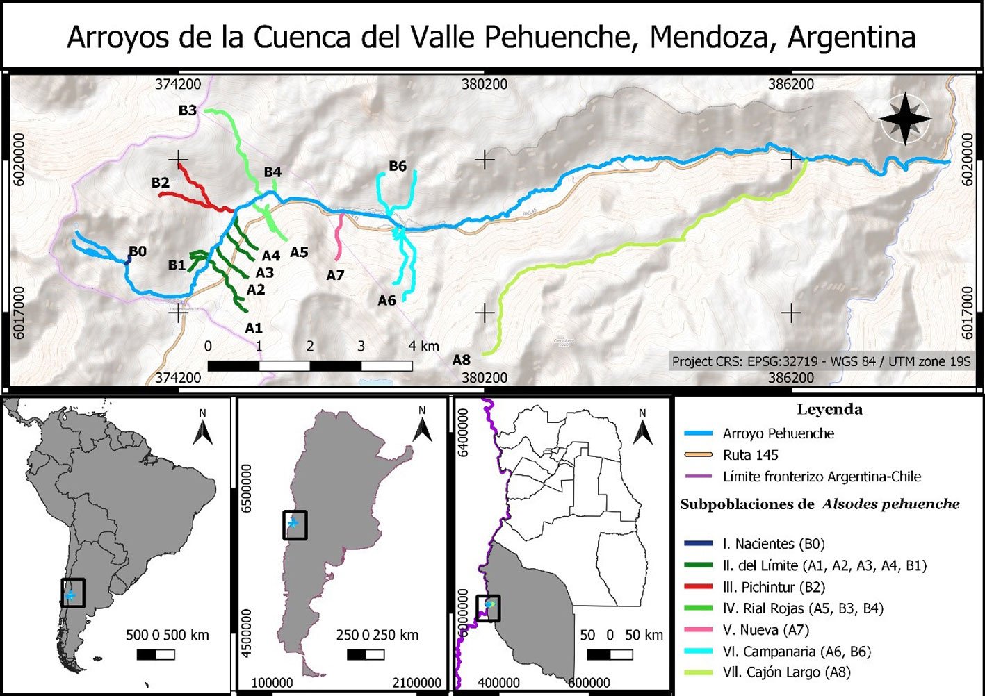
Figura 1. Arroyos muestreados en la cuenca del valle Pehuenche, distribuidos en 7 subpoblaciones locales: I. Nacientes, II. del Límite, III. Pichintur, IV. Rial Rojas, V. Nueva, VI. Campanaria, VII. Cajón Largo. Los arroyos de cada subpoblación se indican con el mismo color.
Se contabilizaron adultos, juveniles y larvas usando la técnica de encuentro visual (Crump y Scott, 1994). Los transectos fueron de rumbo variable siguiendo el curso del arroyo y el ancho fue de 1 m a cada lado del arroyo. Cada transecto se realizó con 2 a 5 observadores. Siguiendo las recomendaciones de Pereyra et al. (2021), al menos un observador tenía experiencia previa y las salidas se programaron en días con condiciones meteorológicas similares: días sin lluvias, mayormente despejados y con vientos leves a moderados.
Para los estadios maduros se registró sexo (macho, hembra e indeterminado). Se registró punto GPS y hora de inicio y de finalización del transecto. Se calcularon las abundancias relativas como individuos/área e individuos/tiempo. El área de los arroyos se consideró como el tramo muestreado en metros multiplicado por 2 m de ancho. Los individuos contabilizados estuvieron a no más de 1 m de distancia del curso del arroyo, cuando éste está claramente definido, y solo se observaron más dispersos en las zonas húmedas de vegas. Para el cálculo de individuos/tiempo se usó el tiempo en minutos de la duración del muestreo (Pereyra et al., 2021).
Adicionalmente, se realizaron muestreos en transectos de 800 m de longitud en los márgenes de la calzada: 10 en la temporada estival de 2021 y 5 en las temporadas siguientes. Este registro se realizó ya que en enero de 2018 se observaron individuos deshidratados o muertos, adyacentes a un cordón o bordillo de 20 cm de altura y 15 cm de ancho.
Se definieron subpoblaciones, siguiendo a Velasco (2018), formadas por un grupo de arroyos que contienen individuos de A. pehuenche, con hábitat adecuado (sensu Corbalán et al., 2010; Correa et al., 2013) y cuya distancia entre ellos no fue mayor a 500 m lineales. De este modo, los 14 arroyos iniciales fueron agrupados en 7 subpoblaciones (fig. 1). Los nombres de las subpoblaciones se relacionan con referencias a las características del paisaje donde se encuentran, excepto la subpoblación denominada Nueva. Se calculó el índice de conectividad (IC) entre subpoblaciones de acuerdo con la fórmula de Lin (2009), modificada por Velasco (2018): IC = A1*(1/D1*T1) + A2*(1/D2*T2), donde Ai es el área (= tamaño poblacional) de la población local vecina hacia el lado i, Di es la distancia a la población local vecina hacia el lado i y Ti la presencia de truchas en hábitat intermedios (presencia multiplica por 2, ausencia multiplica por 1). Para estimar el área correspondiente a cada subpoblación, se usaron las coordenadas GPS de los muestreos de campo y en el caso de las 2 subpoblaciones donde solo se constató presencia, se estimó tamaño del área en Google Earth Pro.
Tabla 1
Temporadas y subpoblaciones en las que se realizaron los muestreos de Alsodes pehuenche. Se indican la cantidad de muestreos realizados en la ruta y los nombres de los arroyos (tipos A, B; P: arroyo Pehuenche) muestreados por subpoblación.
| Temporada | Mes | Quincena primera (1) segunda (2) | Ruta | Subpoblaciones | ||||||
| I | II | III | IV | V | VI | VII | ||||
| 1 (2021) | enero | 1 | 2 | B0 | A1, A2 | |||||
| enero | 2 | 6 | A1, A2, A3, A4 | A5 | A7 | |||||
| febrero | 2 | 1 | A1, A2 | B2 | B3 | |||||
| abril | 2 | 1 | A1, A2 | A5 | A8 | |||||
| 2 (2021-2022) | noviembre | 2 | 1 | A1, B1 | B2 | A5 | A7 | |||
| febrero | 1 | A2 | B3 | |||||||
| marzo | 1 | A1 | B2 | |||||||
| marzo | 2 | B1 | B3 | |||||||
| 3 (2022-2023) | noviembre | 2 | 1 | A5 | ||||||
| diciembre* | 1 | 1 | A1, A3, B1 | B2, B2 | A5-B3 | A6 | A7 | |||
| enero | 1 | 1 | A2, P | A5, B3, P | A6, P | A7, P | ||||
| febrero | 2 | 1 | A1, P | A7, P | ||||||
| marzo | 2 | A3, P | B4, P | B6, P |
Las amenazas que se registraron durante los conteos se consideraron de manera cualitativa, en una escala de 0 a 3, de acuerdo con la intensidad de la amenaza (Velasco, 2018). En la tabla 2 se muestran las amenazas consideradas: 1) la presencia de salmónidos que fueron registrados por encuentro visual; 2) la sequía observada de arroyos que podría ser reversible según la época del monitoreo y cárcavas permanentes cuya profundidad va en aumento; 3) la presencia de ganado, principalmente vacuno y caprino, el primero es el que podría causar mayor impacto debido al mayor uso de las vegas; 4) mortalidad de individuos por causas indeterminadas; 5) la ruta, considerada como una barrera para la dispersión, ya sea porque las alcantarillas no fueron diseñadas como pasos de fauna o porque la altura del cordón o bordillo construido sobre la misma es muy alto para el libre tránsito de ranas juveniles y adultas. Y a pesar de que la ruta representa una barrera, la construcción posterior de rampas, con el objetivo de mitigar este impacto, se considera una acción concreta de conservación. Se registró, además, la presencia de depredadores no acuáticos potenciales y de otras especies de anfibios, pero ninguno de estos casos se considera como amenaza, aunque podrían representar interacciones interespecíficas negativas.
El estado de conservación (EC) relativo de cada subpoblación se obtuvo a partir de la sumatoria de los valores asignados al índice de conectividad y las amenazas (Velasco, 2018). Los valores fueron estandarizados (ECE = EC subpoblación – promedio de todos los EC/desviación estándar de todos los EC) y el valor resultante se multiplicó por -1. Así, los valores negativos de ECE quedaron relacionados con situaciones menos favorables. Se establecieron 2 categorías de prioridades de conservación: baja a media (valores positivos de ECE) y alta (valores negativos de ECE). Los valores altos son los que requieren medidas más urgentes de manejo (Velasco, 2018).
Tabla 2
Variables consideradas para evaluar estado de conservación de las subpoblaciones de Alsodes pehuenche en el valle Pehuenche. IC: Índice de conectividad. Valores 0 a 3 son los que se le asignan a cada variable.
| Variables | 0 | 1 | 2 | 3 |
| Área (m2) | 7,500-10,000 | 5,000-7,500 | 2,500-5,000 | 1,000-2,500 |
| IC1 | 7.51-10 | 5.1-7.5 | 2.51-5 | 0-2.5 |
| Amenazas | ||||
| Efecto especies exóticas: salmónidos | sin | presencia registrada | presencia registrada en más de un conteo | presencia registrada y presencia de anfibio/s con signo de depredación |
| Fragmentación por la ruta | Sin ruta | Sin cordón o bordillo | Con cordón o bordillo y con rampas | Con cordón o bordillo y sin rampas |
| Pérdida de hábitat por sequía/ cárcavas | Sin evidencias de sequía ni cárcavas | Algún arroyo parcialmente seco | Algún arroyo parcialmente seco y/o con presencia cárcavas | Algún arroyo completamente seco y/o presencia de individuos muertos por sequía |
| Efecto del ganado | Sin ganado | Con caprinos | Con vacunos | Con vacunos y cabras |
| Indeterminada | Sin registro de individuos muertos sin causa aparente | Registro de individuos con manchas en la piel | Registro de individuos con manchas y uno muerto sin causa aparente | Registro de más de un individuo muerto sin causa aparente |
1 = Índice de conectividad calculado de acuerdo con Lin (2009), modificado por Velasco (2018).
Se realizaron análisis de los conteos con R versión 4.1.3 y los análisis estadísticos consideraron 0.05 de nivel de significación de alfa. La normalidad de los datos se verificó con la prueba de Shapiro-Wilk. La cantidad de individuos (adultos, juveniles y larvas) por área y por hora no se distribuyó normalmente (W < 0.82934, p < 0.001), por lo que se usaron las pruebas estadísticas no paramétricas de Mann-Whitney-Wilcoxon y de Kruskal-Wallis para 2 grupos y más de 2 grupos, respectivamente. Se evaluó estadísticamente si hubo diferencias entre adultos y juveniles considerados en conjunto versus larvas. También se evaluaron diferencias en relación con variables temporales (temporadas, meses) y espaciales (entre arroyos A y B y entre subpoblaciones). Cuando se obtuvieron diferencias significativas con la prueba de Kruskal-Wallis, se usó el paquete conover.test versión 1.1.5 (2017), basado en Conover-Iman Test para comparaciones múltiples. En todos los casos, los resultados se expresan en mediana, el rango intercuartílico (IQR) como medida de dispersión, los valores mínimos y máximos (min-max) y el tamaño de la muestra (n).
Resultados
Los transectos muestreados alcanzaron un total de 51,292 m lineales recorridos en 181 horas con un esfuerzo de muestreo 12.35 horas/persona. De los 14 arroyos estudiados, todos tuvieron presencia de la especie y el área total fue de 0.04 km². Más de la mitad corresponde a los arroyos denominados A (56.2%).
Cuando se analizaron los conteos respecto de la cantidad de observadores, la correlación de Spearman resultó en valores de rho cercanos a 0, lo que sugiere que no hay correlación lineal (p > 0.05), tanto para individuos postmetamórficos (por área: rho = -0.0427, n = 99; por hora: rho = 0.0975, n = 99), como para larvas (por área: rho = -0.0297, n = 92; por hora rho = -0.0063,
n = 92).
A lo largo del periodo de muestreo se observaron 5.82 adultos y juveniles/área (IQR = 9.27, 0-45 min-max, n = 99) y 13.64 adultos y juveniles/hora (IQR = 30.29, 0-108 min-max, n = 99); 6.24 larvas/área (IQR = 31, 0-175 min-max, n = 92) y 17.76 larvas/hora (IQR = 65, 0-367 min-max, n = 92). La comparación entre estadios muestra menos postmetamórficos que larvas, tanto para los conteos de individuos por área (W = 12.524, p < 0.001) como por hora (W = 26.918, p < 0.001).
Tabla 3
Prioridades de conservación para las subpoblaciones de Alsodes pehuenche en el valle Pehuenche, con base en el tamaño de la población, la conectividad y las amenazas.
| Sub-población | Área (m2) | IC | Amenazas | ECE | PC1 | ||||
| Ruta | Sequía/cárcavas | Ganado | Muertes indet. | Salmónidos | |||||
| I. Nacientes | 4,044 | 8.41 | 0 | 0 | 2 | 0 | 1 | 0.88 | Baja |
| II. del Límite | 5,744 | 8.39 | 2 | 3 | 2 | 2 | 3 | -1.26 | Muy alta |
| III. Pichintur | 5,002 | 9.91 | 0 | 0 | 2 | 3 | 2 | 0.08 | Media |
| IV. Rial Rojas | 6,208 | 6.05 | 1 | 3 | 2 | 1 | 2 | -0.73 | Alta |
| V. Nueva | 2,160 | 9.61 | 1 | 0 | 2 | 3 | 0 | -0.19 | Media |
| VI. Campanaria | 5,860 | 5.26 | 1 | 0 | 1 | 3 | 3 | -0.46 | Media |
| VII. Cajón Largo | 9,550 | 6.64 | 0 | 0 | 1 | 0 | 0 | 1.69 | Muy baja |
1 PC: Prioridad de conservación calculada de acuerdo con Velasco (2018).
Las comparaciones entre las 3 temporadas no mostraron diferencias significativas para ninguno de los grupos estudiados adultos y juveniles/área (H = 1.9935, df = 2, p = 0.369), adultos y juveniles/hora (H = 1.3599, df = 2, p = 0.5066), larvas/área (H = 0.13936, df = 2, p = 0.933) y larvas por hora (H = 0.6051, df = 2, p = 0.7389). Entre meses, la diferencia no fue significativa para larvas (H = 4.5278, df = 5, p = 0.4762 por área, H = 4.0986, df = 5, p = 0.5353 por hora), en cambio para los postmetamórficos solo fue significativa para los conteos por área (H = 13.97, df = 5, p = 0.0158). Los análisis post hoc indican menores cantidades de adultos y juveniles en febrero respecto a diciembre (p = 0.0075) y enero (p = 0.0021), como también en marzo respecto a enero (p = 0.0185, fig. 2).
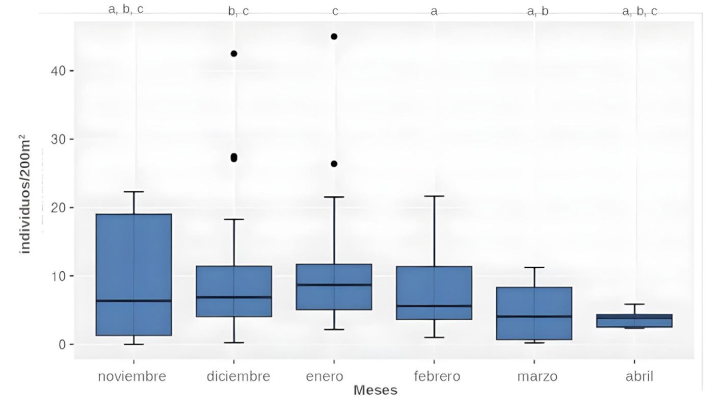
Figura 2. Variación mensual de la abundancia de adultos y juveniles (individuos/200 m2) de Alsodes pehuenche. Los meses con diferentes códigos de letras indican diferencias significativas (p < 0.05).
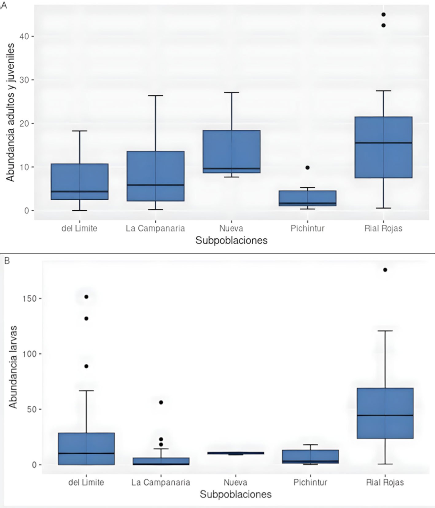
Figura 3. Abundancia de Alsodes pehuenche (individuos/200 m2) entre 5 subpoblaciones. A, Adultos y juveniles; B, larvas. Las subpoblaciones con diferentes códigos de letras indican diferencias significativas (p < 0.05).
De los 14 arroyos del valle Pehuenche con presencia de A. pehuenche, los arroyos A tienen un área de ocupación de 49% respecto de los arroyos B con 51%. Y en los 12 arroyos donde se realizaron conteos por área, éstos fueron mayores en los arroyos A que en los B, tanto para adultos y juveniles (H = 31.977, df = 2, p < 0.001), como para larvas (H = 10.42, df = 2, p = 0.0055).
Se reconocieron 7 subpoblaciones en el valle Pehuenche: Nacientes, del Límite, Pichintur, Rial Rojas, Nueva, Campanaria y Cajón Largo (fig. 1). De éstas, se tienen datos de conteo de 5 (todas, excepto Nacientes y Cajón Largo). Cuando se comparan estas 5 subpoblaciones, se encuentran diferencias significativas tanto para adultos y juveniles/área (H = 17.436, df = 4, p = 0.0016), como para larvas/área (por área H = 23.639, df = 4, p < 0.001). Se registraron más adultos y juveniles en las subpoblaciones Rial Rojas y Nueva, y más larvas en Rial Rojas (fig. 3). Sin embargo, estas diferencias no son significativas cuando se analizan los datos de postmetamórficos/hora (H = 8.8053, df = 5, p = 0.1171) y larvas/hora (H = 4.0986, df = 5, p = 0.5353).
El único lugar donde se encontraron solo larvas fue en una charca de la subpoblación del Límite. Éstas coexistían con larvas y adultos de rana de 4 ojos (Pleurodema bufoninum). Además, esta última especie ha sido observada eventualmente coexistiendo con A. pehuenche en las subpoblaciones Rial Rojas, Campanaria y del Límite. Otras especies registradas durante los muestreos, que se identifican como posibles depredadores de A. pehuenche son el zorro gris (Lycalopex gymnocercus), el chiñe o zorrino (Conepatus chinga), la gaviota capucho café (Chroicocephalus maculipennis) y el águila mora (Geranoaetus melanoleucus).
Aunque la detección de huevos no fue objeto de este estudio, dado que no se realizó búsqueda activa en oquedades ni se manipularon hembras, en noviembre 2022 se observó una masa de 20 huevos aproximadamente, flotando en una pequeña poza de la subpoblación Rial Rojas en época de deshielo. Los huevos no eran pigmentados y cada uno midió entre 6 y 7 mm de diámetro.
Los índices de conectividad calculados para cada una de las subpoblaciones se muestran en la tabla 3. El arroyo Pehuenche representa la principal conexión entre subpoblaciones. En este arroyo se encontraron individuos adultos en la desembocadura de arroyos de primer orden pertenecientes a las subpoblaciones del Límite, Rial Rojas, Nueva y Campanaria (tabla 1). Si bien Cajón Largo tiene relativamente bajo índice de conectividad, el área de esta subpoblación es la mayor de todas.
Se registraron 24 individuos muertos durante el periodo de estudio: 1) 6 individuos adultos —2 hembras, 2 machos y 2 adultos indeterminados— en el mes de enero de la temporada estival 2021 y 2 en la temporada 2022-2023 en los muestreos realizados en la ruta internacional ARG145; 2) 3 individuos —1 adulto indeterminado y 2 larvas— encontrados muertos por desecación sobre el curso de un arroyo de Rial Rojas que mostró una disminución abrupta del caudal luego del deshielo entre noviembre y diciembre 2022; 3) 4 adultos —3 machos y 1 indeterminado— encontrados con signos de depredación (patas traseras lastimadas o mutiladas) al costado o dentro del curso del arroyo donde se registra presencia de salmónidos, esto es, en las subpoblaciones del Límite y Campanaria; 4) 6 adultos —2 machos y 4 indeterminados—, 1 juvenil indeterminado y 2 larvas encontrados muertos sin causa evidente, dentro del curso del arroyo o próximo a éste.
Finalmente, los valores de ECE negativos usados como indicadores, permitieron identificar a las subpoblaciones del Límite y Rial Rojas como unidades de conservación prioritarias, de las cuales la del Límite requiere esfuerzos más urgentes.
Discusión
Corbalán et al. (2010) reportaron 355 individuos de A. pehuenche en 2,500 m lineales (equivalente a 14 individuos/200 m2) en un muestreo realizado en 2008 en arroyos de la subpoblación del Límite. Si se compara ese valor con el obtenido en este estudio para los mismos arroyos en el mismo mes en 2021 (8 individuos/200 m2), el primero es mayor, pero se encuentra dentro del intervalo de variación de este estudio. Cabe mencionar que se usaron 2 técnicas diferentes para el conteo (búsqueda activa de individuos en oquedades durante el día y encuentro visual nocturno, con 3 observadores en los 2 casos), por lo que, con la información disponible actualmente, solo la mortalidad de individuos reportada desde 2008 permite estimar una tendencia poblacional decreciente para esta subpoblación.
En 2 arroyos muy cercanos a la subpoblación del Límite en Chile, Correa et al. (2013) reportaron 20 y 24 adultos/h o 15 y 66 adultos/200 m². Estos últimos datos corresponden a muestreos nocturnos realizados en marzo de 2012, con 4 observadores. La cantidad máxima de adultos por área observados por Correa et al. (2013) es mayor al máximo obtenido en este estudio, lo cual puede deberse a un error de muestreo en solo 30 m lineales, o bien a fluctuaciones poblacionales naturales (Kissel et al., 2020). En arroyos de Rial Moreno, a 21 km al NE de la población del valle Pehuenche, Corbalán et al. (2023) reportaron 26 adultos/hora y 4 juveniles/hora en un muestreo nocturno realizado en enero de 2019, los cuales se encuentran dentro de valores obtenidos en el valle Pehuenche en este estudio.
Durante las 3 temporadas consecutivas muestreadas en este trabajo, no se detectaron cambios significativos para ningún estadio de desarrollo de A. pehuenche. Esto puede deberse a que se trata de un periodo corto en términos de monitoreo. Por lo tanto, es necesario mantener los muestreos para conocer tendencias poblacionales a largo plazo. Por otro lado, la detección de individuos por encuentro visual a lo largo de los arroyos, podría compararse con otros estudios enfocados al monitoreo poblacional de la especie para lograr establecer un óptimo en términos de esfuerzo de muestreo. Dado que estas investigaciones dependen del presupuesto disponible y de limitaciones logísticas (Joseph et al., 2006) principalmente ligadas a la elevada demanda de horas/persona en un ambiente de alta montaña, se debe buscar una estrategia que permita satisfacer tanto la demanda de datos pertinentes para la gestión, como la obtención de información ecológica de calidad (Stephens et al., 2015; Yoccoz et al., 2001).
En relación con la primera acción de conservación llevada a cabo en la población del valle Pehuenche, que consistió en la construcción de 800 m de cordón o bordillo en la ruta y 2 cámaras de infiltración para evitar que la sal vertida en la ruta llegue a los arroyos, provocó la deshidratación y muerte de 18 individuos que fueron encontrados en diciembre de 2017, y 50 en enero de 2018. Posiblemente, la construcción a posteriori de rampas entre el cordón o bordillo y la calzada en febrero de 2018, ha evitado que se vuelvan a registrar mortalidades tan abruptas. Si bien nunca pudo constatarse el uso de las rampas por parte de la especie, las mismas habrían mejorado la conexión entre las secciones superior e inferior de los arroyos. Esto demuestra la necesidad de seguimiento de las acciones de conservación que se llevan a cabo. Pero, por otro lado, si bien la ruta pudo haber provocado una disminución poblacional (Corbalán et al., 2010; IUCN, 2019), el número elevado de individuos muertos registrado en este estudio alerta sobre la necesidad de avanzar en el conocimiento de otras amenazas, como la depredación por salmónidos invasores, el cambio climático y la infección por el hongo quitridio (Batrachochytrium dendrobatidis) de los anfibios.
En este trabajo, de todos los estadios evaluados, las larvas fueron las más abundantes, las más estables en el tiempo y presentaron el mismo patrón de variación que los adultos entre arroyos A y B, y subpoblaciones (fig. 3). Al igual que lo reportado por Corbalán et al. (2010, 2023), se encontraron larvas de diferentes tamaños conviviendo en pozas, pero también se observaron en rápidos, remansos y debajo de la vegetación acuática. Estos resultados son coherentes con la estrategia de especies con desarrollo larval plurianual (Úbeda, 2021). Por otro lado, la menor cantidad de juveniles registrada respecto de adultos podría ser un problema de detectabilidad por su tamaño (Petrovana y Schmidt, 2019), podría corresponder a una segregación por microhábitats según el estadio (Gonwouo et al., 2022), o bien, ser evidencia de una dinámica poblacional particular solo en esta fase de su ciclo de vida (Kissel et al., 2020).
Los muestreos preliminares realizados de día y de noche demuestran que hay arroyos permanentes que solo tienen adultos. Los estudios a futuro podrán determinar las causas que posiblemente puedan estar asociadas con aspectos fisicoquímicos del agua, o a la dispersión de individuos. La información actual permite suponer que las rutas de dispersión de A. pehuenche con base en sus hábitos acuáticos, son los mismos arroyos. Los registros de individuos secos en la ruta, principalmente entre diciembre y enero, al igual que la mayor cantidad de adultos y juveniles registrados en estos meses (fig. 2), podrían estar indicando una mayor dispersión en esa temporada del año.
Los arroyos del valle Pehuenche son los mejores conocidos hasta el momento y el área que ocupan representa solo 6% del área de distribución de A. pehuenche (487.9 km²) reportada por Corbalán et al. (2023). De la misma manera, habiendo considerado en nuestro estudio casi todos los arroyos presentes en el valle Pehuenche, representa 0.8% del área de ocupación total para la especie (4.84 km²; Corbalán et al., 2023). El espacio sin ocupación efectiva de la especie, actualmente, es muy grande (Corbalán et al., 2023), aunque en el pasado pudo haber estado presente en un área mayor si se comparan los registros de presencia en Cajón Grande (Cei y Roig, 1965; Corbalán et al., 2023). Si se considera desde la descripción de la especie en 1965, A. pehuenche ha reducido su área de distribución histórica, lo cual puede deberse a diferentes causas. La depredación por salmónidos en la actualidad podría ser la causa de que la especie haya quedado restringida solo a las zonas altas de las cuencas. Por ello, es necesario conocer la distribución de salmónidos e identificar dónde coexisten estos peces y la rana. Donde esto ocurre en el valle Pehuenche, se registraron adultos muertos de A. pehuenche con signos de depredación. Así, los salmónidos representan una barrera para la dispersión de las ranas, reduciendo la conectividad entre subpoblaciones y dentro de ellas entre arroyos A y B (tabla 3). Como se ha demostrado para otras especies de anfibios, la consecuencia es la disminución del intercambio genético o demográfico (e.g., Kacoliris et al., 2022; Velasco, 2018). Por lo tanto, para conservar las subpoblaciones se requiere asegurar su conectividad, tanto entre las secciones inferior y superior de los arroyos A impactados por la ruta, como dentro de las subpoblaciones entre los arroyos A y B, y entre las subpoblaciones conectadas a través del arroyo Pehuenche.
Las observaciones de campo sugieren que los individuos se distribuyen de manera agrupada a lo largo de los cursos de agua y vegas, no solo las larvas en las pozas, sino también los adultos a lo largo de los arroyos. Esto debe ser evaluado en la etapa reproductiva a inicios de la temporada y al final de ésta, cuando el caudal disminuye y algunos cauces se secan total o parcialmente, donde solo quedan pozas pequeñas con agua. Si este efecto es acentuado por la disminución de cobertura permanente de nieve en la cuenca del Río Grande (Aumassanne et al., 2019), es posible que más arroyos, que todavía mantienen agua hasta el final de la temporada, se sequen como ha ocurrido en los arroyos A3 y A4 de la población del Límite, aumentando así la fragmentación del hábitat. Si A4 no se hubiera secado, las 3 subpoblaciones (del Límite, Pichintur y Rial Rojas) estarían conectadas, formando una sola subpoblación (fig. 1).
Si bien gran parte de las amenazas han sido identificadas (Corbalán et al., 2010, 2023), la mayoría no han sido cuantificadas. Con base en las observaciones realizadas durante los muestreos en este estudio, se sistematizaron las amenazas para cada arroyo y cada subpoblación en el valle Pehuenche (tablas 2, 3). Como resultado de la priorización, las subpoblaciones del Límite y Rial Rojas se identifican como prioritarias para iniciar acciones concretas de conservación. Es posible que ambas sean fragmentos de una población mayor y que hayan estado unidas cuando el arroyo intermedio no estaba seco. En la del Límite se podría iniciar la mitigación de la depredación por salmónidos y reducir los efectos de la ruta. Es necesario continuar con el seguimiento y cuantificación de las amenazas, considerar las aún no evaluadas, tales como las que pueden estar generando las actividades turísticas, el vertido de sal en la ruta, crecidas extraordinarias y otras potenciales como el tendido de líneas de alta tensión, planificada desde el Maule (Chile) al río Diamante (San Rafael, Argentina).
El avance logrado en 20 años de estudios sobre la biología y conservación de este anfibio endémico de Argentina y Chile nos brinda herramientas para sostener acciones concretas de manejo que alivien alguna de las amenazas y que aseguren la viabilidad de las poblaciones a largo plazo. Se espera que un programa de monitoreo anual permita avanzar en el conocimiento de las tendencias poblacionales a largo plazo. Las subpoblaciones del valle Pehuenche son las mejor conocidas hasta el momento y han sufrido disminuciones, fragmentaciones y también extinciones locales. La priorización de su estado de conservación brinda herramientas para implementar acciones necesarias a corto plazo.
Agradecimientos
Por la colaboración en el trabajo de campo, se agradece a estudiantes de la Tecnicatura en Conservación de la Naturaleza Sede Malargüe del IEF Núm. 9-016, especialmente a Julián Rodríguez, Armando Barros, Francisco Jofré y Pablo Lucero; también a estudiantes voluntarios y Graciela Ríos. A Karen Olate por la elaboración del mapa. Y a un revisor anónimo por sus aportes a la primera versión del manuscrito y a los dos revisores que realizaron aportes importantes para mejorar el manuscrito. La investigación se logró gracias al financiamiento del proyecto SIIP 06/M003 Resol. 3978/2022 UNCUYO y aportes personales de investigadoras y estudiantes.
Referencias
Aumassanne, C. M., Beget, M. E., Di Bella, C. M., Oricchio, P. y Gaspari, F. J. (2019). Cobertura de nieve en las cuencas de los ríos Grande y Barrancas (Argentina) y su relación con la morfometría. Revista de Investigación Agropecuaria, 45, 394–403.
Cei, J. M. (1976). Remarks on some neotropical amphibians of the genus Alsodes from southern Argentina. Atti della Società Italiana di Scienze Naturali e del Museo Civico di Storia Naturale di Milano, 117, 159–164.
Cei, J. M. (1980). Amphibians of Argentina. Monitore Zoologico Italiano, N.S. Monografia 2. Florencia: Universitá degli studi di Firenze.
Cei, J. M. y Roig, V. G. (1965). The systematic status and biology of Telmatobius montanus Lataste (Amphibia: Leptodactylidae). Copeia, 4, 421–425.
Corbalán, V., Debandi, G. y Martínez, F. (2010). Alsodes pehuenche (Anura: Cycloramphidae): past, present and future. Cuadernos de Herpetología, 24, 17–23.
Corbalán, V., Debandi, G., Martínez, F. y Úbeda, C. (2014). Prolonged larval development in the critically endangered Pehuenche’s Frog Alsodes pehuenche: implications for conservation. Amphibia–Reptilia, 35, 283–292. http://dx.doi.
org/10.1163/15685381-00002951
Corbalán V., Debandi G., Literas S., Álvarez L., Rivera J. A., Dopazo J. et al. (2023). Newly discovered sites and potential threats for the critically endangered frog, Alsodes pehuenche, in Southern South America. Herpetological Conservation and Biology, 18, 48–56.
Correa, C., Pastenes, L., Iturra, P., Calderón, P., Vásquez, D., Lam, N. et al. (2013). Confirmation of the presence of Alsodes pehuenche Cei, 1976 (Anura, Alsodidae) in Chile: morphological, chromosomal and molecular evidence. Gayana, 77, 117–123. http://dx.doi.org/10.4067/S0717-65382013000200006
Correa, C., Zepeda, P., Lagos, N., Salinas, H., Palma, R. E. y Vásquez, D. (2018). New populations of two threatened species of Alsodes (Anura, Alsodidae) reveal the scarce biogeographic knowledge of the genus in the Andes of central Chile. Zoosystematics and Evolution, 94, 349–358.
Correa, C. J. Morales, C. Schussler y J. C. Ortiz. (2020). An enigmatic population of Alsodes (Anura, Alsodidae) from the Andes of central Chile with three species-level mitochondrial lineages. Mitochondrial DNA Part A DNA Mapping, Sequencing, and Analysis, 31, 25–34. https://doi.org/10.1080/24701394.2019.1704744
Crump, M. L. y Scott, N. J. (1994). Visual encounter surveys. En W. R.Heyer, M. A. Donnelly, R. W. Mc Diarmid, L. A. C. Hayek y M. S. Foster (Eds.). Measuring and Monitoring Biological Diversity Standard Methods for Amphibians (pp. 84–92). Washington D.C.: Smithsonian Institution Press.
Cuevas, C. C. y Formas, J. R. (2003). Cytogenetic analysis of four species of the genus Alsodes (Anura: Leptodactylidae) with comments about the karyological evolution of the genus. Hereditas, 138, 138–147. https://doi.org/10.1034/j.1601-5223.2003.01677.x
Garreaud, R., Vuille, M., Compagnucci, R. y Marengo, J. (2009). Present-day south american climate. Palaeogeography, Palaeoclimatology, Palaeoecology, 281, 180–195. http://dx.
doi.org/10.1016/j.palaeo.2007.10.032
Ghirardi, R., Levy, M. G., López, J. A., Corbalán, V., Steciow, M. M. y Perotti, M. G. (2014). Endangered amphibians infected with the chytrid fungus Batrachochytrium dendrobatidis in austral temperate wetlands from Argentina. Herpetological Journal, 24, 129–133.
Gonwouo, N. L. Schäfer, M. y Tsekané, S. J. (2022). Goliath frog (Conraua goliath) abundance in relation to frog age, habitat, and human activity. Amphibian and Reptile Conservation, 16, e319.
Grant, E. H. C., Miller, D. A. y Muths, E. (2020). A synthesis of evidence of drivers of amphibian declines. Herpetologica, 76, 101–107. https://doi.org/10.1655/0018-0831-76.2.101
Green D. M., Lannoo M. J., Lesbarrères D. y Muths E. (2020). Amphibian population declines: 30 years of progress in confronting a complex problem. Herpetologica, 76, 97–100. https://doi.org/10.1655/0018-0831-76.2.97
Herrera, F. y Velásquez, N. A. (2016a). Dimorfismo sexual en Alsodes pehuenche Cei 1976 (Amphibia, Anura, Alsodidae). Boletín Chileno de Herpetología, 3, 4–6.
Herrera, F. y Velásquez, N. A. (2016b). Uso de cuevas en Alsodes pehuenche Cei 1976 (Amphibia, Anura, Alsodidae). Boletín Chileno de Herpetología, 3, 17–20.
Jensen, I. S., Haugen, V. F. y Skålin, R. (2007). Yr. Norwegian Meteorological Institute and the Norwegian Broadcasting Corporation. Recuperado el 15 de agosto, 2024 de https://www.yr.no/nb
Joseph, L. N., Field, S. A., Wilcox, C. y Possingham, H. P. (2006). Presence-absence versus abundance data for monitoring threatened species. Conservation Biology, 20, 1679–1687. https://doi.org/10.1111/j.1523-1739.2006.00529.x
Kacoliris, F. P., Berkunsky, I., Acosta, J. C., Acosta, R., Agostini, M. G., Akmentins, M. et al. (2022). Current threats faced by amphibian populations in the southern cone of South America. Journal for Nature Conservation, 69, 126254. https://doi.org/10.1016/j.jnc.2022.126254
Kissel, A. M., Tenan, S. y Muths, E. (2020). Density dependence and adult survival drive dynamics in two high elevation amphibian populations. Diversity, 12, 478.
Lin, J. P. (2009). The functional linkage index: a metric for measuring connectivity among habitat patches using least-cost distances. Journal of Conservation Planning, 5, 28–37.
Llano, C., Durán, V., Gasco, A., Reynals, E. y Zárate, M. S. (2021). Traditional puesteros´ perceptions of biodiversity in semi-arid Southern Mendoza, Argentina. Journal of Arid Environments, 192, 104553. https://doi.org/10.1016/j.ja
ridenv.2021.104553
Luedtke, J. A., Chanson, J., Neam, K., Hobin L., Maciel, A. O., Catenazzi, A. et al. (2023). Ongoing declines for the world’s amphibians in the face of emerging threats. Nature, 622, 308–314. https://doi.org/10.1038/s41586-023-06235-w
Luja, V., Rodríguez-Estrella, H. R., Schaub, M. y Schmidt, B. R. (2015). Among-population variation in monthly and annual survival of the Baja California treefrog, Pseudacris hypochondriaca curta, in desert oases of Baja California Sur, Mexico. Herpetological Conservation and Biology, 10, 112–122.
Pereyra, L. C., Etchepare, E. y Vaira, M. (2021). Manual de técnicas y protocolos para el relevamiento y estudio de anfibios de Argentina. San Salvador de Jujuy: Editorial de la Universidad Nacional de Jujuy.
Petrovana, S. O. y Schmidt, B. R. (2019). Neglected juveniles; a call for integrating all amphibian life stages in assessments of mitigation success (and how to do it). Biological Conservation, 236, 252–260. https://doi.org/10.1016/j.biocon.
2019.04.016
Piñeiro, A., Fibla, P., López, C., Velásquez, N. y Pastenes, L. (2020). Characterization of an Alsodes pehuenche breeding site in the Andes of central Chile. Herpetozoa, 33, 21–26. https://doi.org/10.3897/herpetozoa.33.e49268
Pollock, J. E. (2006). Detecting population declines over large areas with presence-absence, time-to-encounter, and count survey methods. Conservation Biology, 20, 882–892. https://doi.org/10.1111/j.1523-1739.2006.00559.x
Prado, W. S., Meriggi, J., Martínez, F. y Corbalán, V. (2019). Ampliación del área de distribución de Alsodes pehuenche en Argentina. Revista del Museo de La Plata, 4 (Suplem.), 1R–117R.
Rivera, J. A., Marianetti, G. y Hinrichs, S. (2018). Validation of CHIRPS precipitation dataset along the Central Andes of Argentina. Atmospheric Research, 213, 437–449. https:
//doi.org/10.1016/j.pce.2022.103184
Stephens, P. A., Pettorelli, N., Barlow, J., Whittingham, M. J. y Cadotte, M. W. (2015). Management by proxy? The use of indices in applied ecology. Journal of Applied Ecology, 52, 1–6. https://doi.org/10.1111/1365-2664.12405
Úbeda, C. (2021). Estrategias reproductivas, hábitats y otros aspectos ecológicos de los anfibios altoandinos en la vertiente oriental de la Cordillera de los Andes. Boletín Chileno de Herpetología, 8, 10–21.
UICN (Unión Internacional para la Conservación de la Naturaleza), Species Survival Commission Amphibian Specialist Group. (2019). Alsodes pehuenche. IUCN Red List of threatened species, 2019. https://www.iucnredlist.org
Vaira, M., Akmentins, M., Attademo, M., Baldo, D., Barrasso, D., Barrionuevo, S. et al. (2012). Categorización del estado de conservación de los anfibios de la República Argentina. Cuadernos de Herpetología, 26 (Suplem. 1), 131–159.
Vaira, M., Pereyra, L. C., Akmentins M. S. y Bielby, J. (2017). Conservation status of Amphibians of Argentina: An update and evaluation of national assessments. Amphibian y Reptile Conservation, 11, e135.
Velasco, M. A. (2018). Dinámica poblacional y conservación de la ranita del Valcheta (Pleurodema somuncurense) (Cei, 1969), Patagonia, Argentina (Tesis doctoral). Universidad Nacional de La Plata, La Plata, Buenos Aires.
Velasco, M. A., Kacoliris, F. P., Berkunsky, I., Quiroga, S. y Williams, J. D. (2016). Current distributional status of the critically endangered Valcheta frog: implications for conservation. Neotropical Biology and Conservation, 11, 110–113. http://dx.doi.org/10.4013/nbc.2016.112.08
Vidal, M. A., Henríquez, N., Torres-Díaz, C., Collado, G. y Acuña-Rodríguez, I. S. (2024). Identifying strategies for effective biodiversity preservation and species status of Chilean amphibians. Biology, 13, 169. https://doi.org/10.33
90/biology13030169
Yoccoz, N. G., Nichols, J. D. y Boulinier, T. (2001). Monitoring of biological diversity in space and time. Trends in Ecology and Evolution, 16, 446–453. https://doi.org/10.1016/S0169-
5347(01)02205-4
Zarco, A., Corbalán, V. y Debandi, G. (2020). Depredación por truchas arcoíris invasoras en la rana de pecho espinoso Pehuenche, en peligro crítico. Journal of Fish Biology, 98, 878-880. https://doi.org/10.1111/jfb.14401

Priority areas for conservation based on endemic vascular plant species and their biocultural attributes: a case study in Sinaloa, Mexico
C. Rocío Álamo-Herrera a, María Clara Arteaga a, *, Rafael Bello-Bedoy b
a Instituto Politécnico Nacional, Centro Interdisciplinario de Investigación para el Desarrollo Integral Regional, Unidad Durango, Sigma No. 119, Fracc. 20 de Noviembre II, 34234 Victoria de Durango, Durango, Mexico
b Universidad de Guadalajara, Centro Universitario de Ciencias Biológicas y Agropecuarias, Cátedras Conahcyt-Universidad de Guadalajara, Camino Ramón Padilla Sánchez No. 2100, 45200 Zapopan, Jalisco, Mexico
*Corresponding author: d1j17kk@hotmail.com (J.F. Pío-León)
Received: 20 February 2024; accepted: 02 July 2024
Abstract
Endemic vascular plants are one of the main biodiversity indicators used to propose priority conservation areas. The richness of endemic species and corrected and weighted endemism are the most frequently used criteria, while anthropogenic or biocultural factors such as ethnobotanical value or ecological vulnerability are seldom considered. This work proposes priority conservation areas for Sinaloa, Mexico, considering the richness of its endemic species, corrected and weighted endemism, as well as ethnobotanical value, protection status, and the Priority Conservation Index (PCI). The analysis was performed in a 19 × 19 km grid and included 247 records of 78 species. The areas proposed when considering only the richness of endemic species and the weighted endemism coincided with previously known areas of high biodiversity in the state, which are areas of high collection effort and low anthropogenic impact. When considering the ethnobotanical value and protection status, the areas identified included those with greater anthropogenic impact, which contained species of biocultural and economic importance. When the PCI was used, both of these types of regions were identified. We therefore recommend this index as a better indicator to select priority areas.
Keywords: Conservation index; Ebenopsis caesalpinioides; Ethnobotanical value; Protected Natural Areas; Priority species; Stenocereus martinezii
© 2024 Universidad Nacional Autónoma de México, Instituto de Biología. Este es un artículo Open Access bajo la licencia CC BY-NC-ND
(http://creativecommons.org/licenses/by-nc-nd/4.0/).
Áreas prioritarias para la conservación con base en especies de plantas vasculares endémicas y sus atributos bioculturales: un estudio de caso en Sinaloa, México
Resumen
Las plantas vasculares endémicas son uno de los principales indicadores empleados para proponer áreas prioritarias de conservación. La riqueza de especies endémicas y el endemismo ponderado y corregido son frecuentemente incluidos en los análisis, mientras que aspectos antropogénicos o bioculturales como el valor etnobotánico o la vulnerabilidad ecológica son poco considerados. Este trabajo propone áreas prioritarias de conservación para Sinaloa, México, considerando su riqueza de especies endémicas, endemismo ponderado y corregido, así como el valor etnobotánico, estatus de protección e índice prioritario de conservación (IPC). El análisis se realizó en cuadrículas de 19 × 19 km e incluyó 274 registros de 78 especies. Las áreas resultantes, considerando únicamente la riqueza de especies y el endemismo ponderado, coinciden con áreas previamente conocidas por su alta biodiversidad en el estado, mismas que poseen altos esfuerzos de colectas y bajos impactos antropogénicos. Por el contrario, cuando se consideró el valor etnobotánico y el estatus de protección, las áreas prioritarias incluyen zonas con alto impacto antropogénico, pero con presencia de especies con importancia biocultural y valor económico. Empleando el IPC se identificaron ambos tipos de regiones; en consecuencia, recomendamos este índice como un mejor indicador para seleccionar áreas prioritarias.
Palabras clave: Índice de conservación; Ebenopsis caesalpinioides; Valor etnobotánico; Áreas naturales protegidas; Especies prioritarias; Stenocereus martinezii
Introduction
Plants are essential organisms for maintaining the equilibrium of ecosystems and life on Earth. They provide the vast majority of the ecosystem and subsistence services that humans need to survive, including food, medicine, shelter, oxygen, carbon capture, and soil retention. Caring for plants is therefore an act of self-preservation (Raven, 2018). However, over 50% of the terrestrial vegetation on Earth is severely or moderately altered (Bradshaw et al., 2021).
Mexico is the country with the third to fifth highest plant richness, with more than 23,000 species, half of which are endemic (Conabio, 2023a; Villaseñor & Meave, 2022). However, despite 12% of Mexican territory being decreed as Protected Natural Area, it is estimated that between 37 and 50% of the nation’s land area has been impacted by human activities and that the majority of well-conserved areas are located in desert, semi-desert, and high mountain areas that are difficult to access (González-Abraham et al., 2015; Mora, 2019). Two of the largest and most biodiverse ecosystems in the country —dry forest and temperate forest— have suffered total degradation of 37 and 26% of their cover, respectively (Conabio, 2023b; Ulloa-Ulloa et al., 2017). The main causes of this deforestation have been agriculture and infrastructure development, both in Mexico specifically and worldwide (González-Abraham et al., 2015; Laso-Bayas et al., 2022).
One of the main analytical approaches used to propose priority conservation areas is grid analysis, which identifies centers of high biodiversity (“hotspots”) using criteria such as species richness, richness of endemic species, weighted endemism (WE), presence of threatened species, diversity of specific taxa (families or genera), or phylogenetic richness (Gutiérrez-Rodríguez et al., 2022; Maassoumi & Ashouri, 2022; Mehta et al., 2023; Murillo-Pérez et al., 2022; Qin et al., 2022; Sosa & De-Nova, 2012; Vargas-Amado et al., 2020; Villaseñor et al., 2022). The richness of endemic species in particular has the advantage of using a more precise (though smaller) database than the other aforementioned criteria for grid analysis to indicate conservation priority areas.
On the other hand, other indices can be used to propose conservation priority species based on their ethnobotanical or biocultural value, or the degree of threat they face due to use (e.g., Value of Use, Frequency of Use, Conservation Index) (De Lucena et al., 2013; Dhar et al., 2000; Mehta et al., 2023; Pío-León et al., 2023). However, these indices are not usually included in grid richness analyses to select priority conservation areas. These indices weight each species’ value based on its conservation priority, such that a priority conservation area would be determined not just by the total number of species or endemism, but also by their qualities.
Pío-León et al. (2023) compiled a list of the vascular plant species of Sinaloa and proposed some priority conservation areas based on the presence of 2 or more endemic species. In addition, the authors proposed a Priority Conservation Index (PCI) for each species based on its ethnobotanical value and ecological vulnerability, considering characteristics such as its distribution, habitat, and anthropogenic threats. In this index, species with high ethnobotanical value, slow growth (arboreal habit), threatened habitat (near to agricultural zones), and small distribution area (1 or a few known localities), have higher priority than those with no known ethnobotanical value, rapid growth (herbs), inaccessible habitat (cliffs or steep slopes), and wide distribution. The PCI was calculated with the formula:
PCI= D + H + Fv + Am + VE + Vc
where D is distribution; H, habitat; Fv, life form or habit (Spanish abbreviation); Am, degree of threat to their populations; VE, ethnobotanical value, and Vc, commercial value. However, that work did not perform a grid richness analysis to incorporate the values of these indices with traditional algorithms such as WE.
In the present work, we propose priority conservation areas in Sinaloa considering 3 types of algorithms: 1) richness of endemic species, WE, and corrected weighted endemism (CWE); 2) ethnobotanical value, protection status (NOM-059-SEMARNAT-2010 or IUCN) and PCI, and 3) the combination of 1) and 2). We hypothesized that incorporating those anthropogenic and biocultural attributes would modify the priority conservation areas selected since they will not necessarily correspond to the areas of the highest species richness.
Materials and methods
Sinaloa is located in northwestern Mexico, bordered on the east by the Sierra Madre Occidental (SMO) and on the west by the Pacific Ocean. According to Wiken et al. (2011), the main level III ecoregions that compose it are: 1) Sinaloa and Sonora Hills and Canyons with Xeric Shrub and Low Tropical Deciduous Forest (SS-TDF) (50%, 27,568 km2), which is located in the low parts of the SMO; 2) Sinaloa Coastal Plain with Low Tropical Thorn Forest and Wetland (S-TF) (29%, 15,612 km2), located in the lowlands near the coast, from the south-central portion northward; and 3) SMO with Conifer, Oak, and Mixed Forests (PQF) (15.78%, 8,681 km2) in the high parts of the western slope of the SMO (Fig. 1). It has been estimated that 4,000 species of vascular plants, nearly 80 of them endemic, occur in Sinaloa (Pío-León et al., 2023; Vega-Aviña et al., 2021). However, a large part of the coastal territory has been converted to agricultural land (~ 28,000 km2) (INEGI, 2023), resulting in severely fragmented habitats.
The database was based on the file generated by Pío-León et al. (2023) with some updates (Table 1). We incorporated recently described species (until October 2023) and removed species and collections that lacked reliable geographic coordinates. In addition, we prepared a matrix of weighted values considering the ethnobotanical value (E; 1 = documented use, 0 = no documented use), inclusion in a risk category (R) by the NOM-059-SEMARNAT-2010 (Semarnat, 2019) or IUCN (2023) (1 = included in at least 1 category, 0 = not included), and the value of the Conservation Priority Index (PCI), using the values reported by Pío-León et al. (2023) (Table 1). For the PCI, we assigned values according to their quartile position: 4 (upper quartile), 3 (second quartile), 2 (third quartile), and 1 (lower quartile). From these data, we formed 3 analysis groups: 1) biocultural value (E+R; 0 to 2), 2) PCI value (1 to 4), and 3) PCI + R (1 to 5).
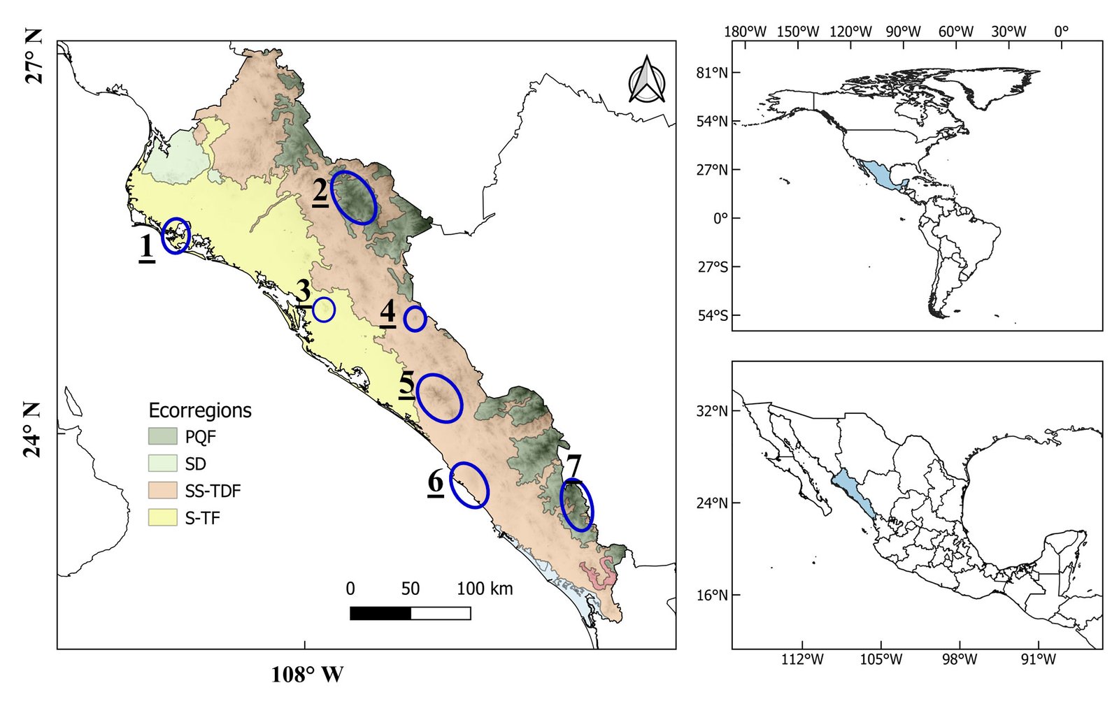
Figure 1. Sinaloa state, Mexico, its main ecoregions level III (Wiken et al., 2011), and the regions of endemism according to Pío-León et al. (2023). Ecoregions: PQF = Conifer, Oak, and Mixed Forests of the Sierra Madre Occidental; SD = Sonoran Desert; SS-TDF = Sinaloa and Sonora Hills and Canyons with Xeric Shrub and Low Tropical Deciduous Forest; S-TF = Sinaloa Coastal Plain with Low Tropical Thorn Forest and Wetlands. Regions of endemism: 1 = Maviri-Topolobampo, 2 = Surutato region, 3 = Cerro Tecomate, 4 = Cerro Colorado, 5 = Sierra Tacuichamona, 6 = Meseta de Cacaxtla, 7 = Sierra de Concordia.
Table 1
List of endemic species of Sinaloa considered for this study and their scores by attributes. E = Ethnobotanical value; R = species with conservation status by the NOM-059-SEMARNAT-2010 or the IUCN (risk); PCI = Priority Conservation Index according to their quartile position.
| Especies | E | R | PCI | E+R | PCI+R |
| Acourtia gentryi L. Cabrera | 0 | 0 | 2 | 0 | 2 |
| Acourtia sinaloana B.L. Turner | 0 | 0 | 1 | 0 | 1 |
| Ageratina concordiana B.L. Turner | 0 | 0 | 2 | 0 | 2 |
| Albizia ortegae Britton & Rose | 0 | 0 | 3 | 0 | 3 |
| Aloysia nahuire A.H. Gentry & Moldenke | 1 | 0 | 4 | 1 | 5 |
| Anemia brandegeei Davenp. | 0 | 0 | 1 | 0 | 1 |
| Arachnothryx sinaloae Borhidi | 0 | 0 | 2 | 0 | 2 |
| Bastardiastrum tarasoides Fryxell | 0 | 0 | 2 | 0 | 2 |
| Bastardiastrum wissaduloides (Baker f.) Bates | 0 | 0 | 1 | 0 | 1 |
| Bletia santosii H. Ávila, J.G. González & Art. Castro | 0 | 0 | 2 | 0 | 2 |
| Bourreria franciscoi Pío-León & Vega | 0 | 0 | 3 | 0 | 3 |
| Bourreria ritovegana Pio-León, M.G. Chávez & L.O. Alvarado | 0 | 0 | 3 | 0 | 3 |
| Bouvardia sinaloae Borhidi & E. Martínez | 0 | 0 | 2 | 0 | 2 |
| Calliandra estebanensis H.M. Hern. | 0 | 0 | 2 | 0 | 2 |
| Carlowrightia fuertensis T.F. Daniel | 0 | 0 | 3 | 0 | 3 |
| Castilleja racemosa (Breedlove & Heckard) T.I. Chuang & Heckard | 0 | 0 | 3 | 0 | 3 |
| Chrysactinia lehtoae D.J. Keil | 0 | 0 | 2 | 0 | 2 |
| Cnidoscolus sinaloensis Breckon ex Fern.Casas | 0 | 1 | 3 | 1 | 4 |
| Cochemiea thomasii García-Mor., Rodr. González, J. García-Jim. & Iamonico | 0 | 0 | 2 | 0 | 2 |
| Coutaportla helgae Pío-León, Torr.-Montúfar & H. Ávila | 0 | 0 | 1 | 0 | 1 |
| Coutaportla lorenceana Torr.-Montúfar, H. Ochot. & Art.Castro | 0 | 0 | 2 | 0 | 2 |
| Croton ortegae Standl. | 0 | 0 | 3 | 0 | 3 |
| Ctenodon rosei Morton | 0 | 0 | 3 | 0 | 3 |
| Cuphea delicatula Brandegee | 0 | 0 | 2 | 0 | 2 |
| Cyclanthera monticola Gentry | 0 | 0 | 2 | 0 | 2 |
| Dioscorea sinaloensis O. Téllez | 0 | 0 | 2 | 0 | 2 |
| Dryopetalon breedlovei (Rollins) Al-Shehbaz | 0 | 0 | 1 | 0 | 1 |
| Ebenopsis caesalpinioides (Standl.) Britton & Rose | 1 | 1 | 4 | 2 | 5 |
| Echeveria coppii Moran ex Gideon F.Sm. & Bischofberger | 0 | 0 | 2 | 0 | 2 |
| Echeveria juliana Reyes, González-Zorzano & Kristen | 0 | 0 | 1 | 0 | 1 |
| Echeveria kimnachii J. Meyrán & R. Vega | 0 | 0 | 1 | 0 | 1 |
| Epidendrum petacaense Hágsater, J. Duarte & Pío-León | 0 | 0 | 2 | 0 | 2 |
| Eryngiophyllum rosei Greenm. | 0 | 0 | 2 | 0 | 2 |
| Frangula surotatensis (Gentry) A. Pool | 0 | 0 | 2 | 0 | 2 |
| Graptopetalum sinaloensis Vega | 0 | 0 | 1 | 0 | 1 |
| Guardiola stenodonta S.F. Blake | 0 | 0 | 1 | 0 | 1 |
| Helicteres vegae Cristóbal | 0 | 0 | 3 | 0 | 3 |
| Heliopsis sinaloensis B.L. Turner | 0 | 0 | 2 | 0 | 2 |
| Table 1. Continued | |||||
| Especies | E | R | PCI | E+R | PCI+R |
| Hofmeisteria sinaloensis Gentry | 0 | 0 | 1 | 0 | 1 |
| Indigofera sinaloensis M. Sousa & Cruz Durán | 0 | 0 | 2 | 0 | 2 |
| Ipomopsis monticola J.M. Porter & L.A. Johnson | 0 | 0 | 2 | 0 | 2 |
| Iresine arenaria Standl. | 0 | 0 | 1 | 0 | 1 |
| Koanophyllum concordianum B.L. Turner | 0 | 0 | 2 | 0 | 2 |
| Lasianthaea gentryi B.L. Turner | 0 | 0 | 2 | 0 | 2 |
| Lasianthaea ritovegana B.L. Turner | 0 | 0 | 1 | 0 | 1 |
| Licania mexicana Lundell | 0 | 0 | 2 | 0 | 2 |
| Lobelia macrocentron (Benth.) T.J. Ayers | 0 | 0 | 2 | 0 | 2 |
| Lopezia conjugens Brandegee | 0 | 0 | 1 | 0 | 1 |
| Lopezia sinaloensis Munz | 0 | 0 | 1 | 0 | 1 |
| Lupinus gentryanus C.P. Sm. | 0 | 0 | 2 | 0 | 2 |
| Lupinus howard-scottii C.P. Sm. | 0 | 0 | 2 | 0 | 2 |
| Lupinus sinaloensis C.P. Sm. | 0 | 0 | 2 | 0 | 2 |
| Mariosousa gentryi Seigler & Ebinger | 0 | 0 | 3 | 0 | 3 |
| Mimosa coelocarpa B.L. Rob. | 0 | 0 | 3 | 0 | 3 |
| Mitracarpus aristatus Borhidi & Lozada-Pérez | 0 | 0 | 2 | 0 | 2 |
| Molinadendron sinaloense (Standl. & Gentry) P.K. Endress | 0 | 1 | 3 | 1 | 4 |
| Pavonia gentryi Fryxell | 0 | 0 | 2 | 0 | 2 |
| Peniocereus papillosus (Britton & Rose) U. Guzmán | 0 | 0 | 2 | 0 | 2 |
| Periptera trichostemon Bullock | 0 | 0 | 2 | 0 | 2 |
| Perityle canescens Everly | 0 | 0 | 1 | 0 | 1 |
| Perityle grandifolia Brandegee | 0 | 0 | 1 | 0 | 1 |
| Perityle stevensii B.L. Turner | 0 | 0 | 1 | 0 | 1 |
| Physalis vestita Waterf. | 0 | 0 | 3 | 0 | 3 |
| Pitcairnia monticola Brandegee | 0 | 0 | 1 | 0 | 1 |
| Polygala polyedra Brandegee | 0 | 0 | 1 | 0 | 1 |
| Psacalium quercifolium H.Rob. & Brettell | 0 | 0 | 2 | 0 | 2 |
| Salvia beltraniorum J.G.González, Pío-León & Art.Castro | 0 | 0 | 2 | 0 | 2 |
| Salvia trichostephana Epling | 0 | 0 | 2 | 0 | 2 |
| Sedum copalense Kimnach | 0 | 0 | 1 | 0 | 1 |
| Stenocereus martinezii (J.G. Ortega) Bravo | 1 | 1 | 4 | 2 | 5 |
| Stevia concordiana B.L. Turner | 0 | 0 | 2 | 0 | 2 |
| Sysyrinchium jacquelineanum Art.Castro, H. Ávila & J.G. González | 0 | 0 | 1 | 0 | 1 |
| Tibouchina thulia Todzia | 0 | 0 | 1 | 0 | 1 |
| Tillandsia mazatlanensis Rauh | 0 | 0 | 2 | 0 | 2 |
| Tillandsia occulta H. Luther | 0 | 0 | 2 | 0 | 2 |
| Verbesina microcarpa S.F. Blake | 0 | 0 | 2 | 0 | 2 |
| Verbesina ortegae S.F. Blake | 0 | 0 | 2 | 0 | 2 |
| Verbesina sinaloensis B.L. Turner | 0 | 0 | 2 | 0 | 2 |
Richness of endemism (SR), weighted endemism (WE), and corrected weighted endemism (CWE). The richness of endemic species was quantified in 19 × 19 km cells (361 km2), dividing Sinaloa into 195 cells. The cell size used was determined according to the criterion of Oyala (2020). Endemic species richness was quantified as the total number of endemic species whose distribution includes the cell. Endemism was evaluated using the WE and CWE indices. The WE score for each cell was obtained by summing, for each species present in the cell, the inverse of the number of cells in which the species occurs; thus, a high WE value indicates cells that contain more species with restricted distributions (i.e., that are found in few other cells), while low WE values indicate cells that mostly contain widely distributed species (i.e., species that are also present in other cells). The CWE is similar, but additionally corrects for potential biases due to differences in overall richness by dividing the value of the WE by the number of species present in the cell (Laffan & Crisp, 2003). The 3 parameters (SR, WE, and CWE) were estimated in the program Biodiverse v.2.0 (Laffan et al., 2010). Geoprocessing of the data was performed in QGIS 3.4.8 (QGIS.org, 2019).
Endemism weighted by biocultural attributes and PCI. In addition to SR, WE, and CWE analysis, endemism weighted by biocultural attributes was evaluated using 2 sets of attribute/parameter combinations, each resulting in 3 maps, 9 in total (Fig. 2). The first set included the species richness plus the biocultural values, resulting in the following 3 combinations: species richness plus biocultural value (SR+E+R), species richness plus PCI (SR+PCI), and PCI plus the risk category (SR+PCI+R). The second set did not consider species richness, resulting in the combinations of biocultural value (E+R), PCI, and PCI+R. For this second set of analyses, only species that fulfilled the relevant criteria were included (e.g., the E+R combination included only species that had ethnobotanical value and are included in a risk category). As such, in the first set of maps, a priority conservation area depended by the number of species present and their qualities (e.g., species with ethnobotanical value or species with protected status), while in the second only the species’ qualities were considered.
The final priority conservation areas were based on the consensus map of the 9 different endemism maps. The consensus areas took into account only the cells that had the highest possible value of the relevant variables in at least 1 of the 9 previously generated endemism maps. The consensus values were obtained by summing the number of times each cell had the highest possible value in each of the endemism maps, such that the highest possible consensus value was theoretically 9 (the cell had the highest possible value in all maps), and the minimum value was 1 (maximal value in only 1 map). The consensus map was also overlayed with Protected Natural Areas and Priority Terrestrial Regions, land use, and bioclimatic corridors.
Results
Occurrence, conservation (risk) status, and ethnobotanical uses of the endemic species of Sinaloa. The database contained 247 records of 78 species, 30 families, and 61 genera. For 48 of the genera (78.7%), only 1 species of the genus was present. The majority of the records were distributed in the central to the southern region of the state, near the coast, in the Meseta de Cacaxtla Natural Protected Area and the area between the former and Sierra de Tacuichamona, as well as in the Concordia and Surutato mountains of the SMO (Fig. 3; regions 6, 5, and 2, in Figure 1). The 2 level III ecoregions best represented were SS-TDF (166 records/ 40 species) and the PQF (53/ 37), followed by the S-TF (17/ 8) (Fig. 3a). Sixty-nine percent of the records fell outside of the polygons of Protected Natural Areas or Priority Terrestrial Conservation Regions (Fig. 3B). Sixty-eight percent of the species (53) were known from a single locality (either a single collection or collections from locations that are very close to each other).

Figure 2. Flowchart of the endemism analysis to select priority areas in Sinaloa, Mexico.
Only 4 species (Cnidoscolus sinaloensis, Ebenopsis caesalpinioides, Molinadendron sinaloense, and Stenocereus martinezii) of the 78 analyzed are found in some risk category (Table 1). All 4 are considered endangered (EN) by the IUCN, while only Stenocereus martinezii is included in NOM-059-SEMARNAT-2010, under the category of special protection (Pr). Only 3 species have well-documented ethnobotanical uses: Aloysia nahuire (aromatic and medicinal tea), Ebenopsis caesalpinioides (edible seeds, occasional commercial value), and Stenocereus martinezii (edible fruits, commercial value). One additional species, Lupinus gentryianus, was noted in the type collection to be used as an anti-parasitic for livestock; however, this plant is only known from that locality, and this use has not since been confirmed, so it was not considered.
The different patterns of endemism are shown in Figure 4. The overall richness of endemism (Fig. 4A) showed 2 main areas —1 in the northern part of the Sierra de Concordia (region 7, Fig. 1) and the other in the western part of the Sierra de Tacuichamona (region 5, Fig. 1)— as well as 3 secondary areas located in the Sierra de Surutato (region 2, Fig. 1), Cerro Colorado (region 4, Fig. 1), and the southern part of the Sierra de Concordia. The WE (Fig. 4B) showed a similar pattern in richness but with an increase in the priority levels of the Sierra de Surutato and a decrease by 1 level for the Tacuichamona and Cerro Colorado. The CWE (Fig. 4C) showed several priority areas more scattered across the state than the WE, mainly in the SMO, corresponding to the majority of the species known from a single locality; however, compared with WE, there was a greater concentration of high-priority cells toward the northern part of the state, near southern Sonora, in the area around the Sierra de Barobampo and Hills of Topolobampo (region 1, Fig. 1).

Figure 3. Records of endemic species in Sinaloa overlayed onto: level III ecoregions (Wiken et al., 2011; definitions in Figure 1) (A) and Protected Natural Areas (PNA) and Priority Terrestrial Regions (B). Categories of Protected Natural Areas: PNAS = state; PNAM = municipal; PNAF = federal; PTR = Priority Terrestrial Regions.
Figure 4. Endemism areas of vascular plants in Sinaloa, Mexico, according to the calculated index values (A-I): SR = endemic species richness; WE = weighted endemism; CWE = corrected weighted endemism; E = ethnobotanical value; R = species with protection status; PCI = Priority Conservation Index.
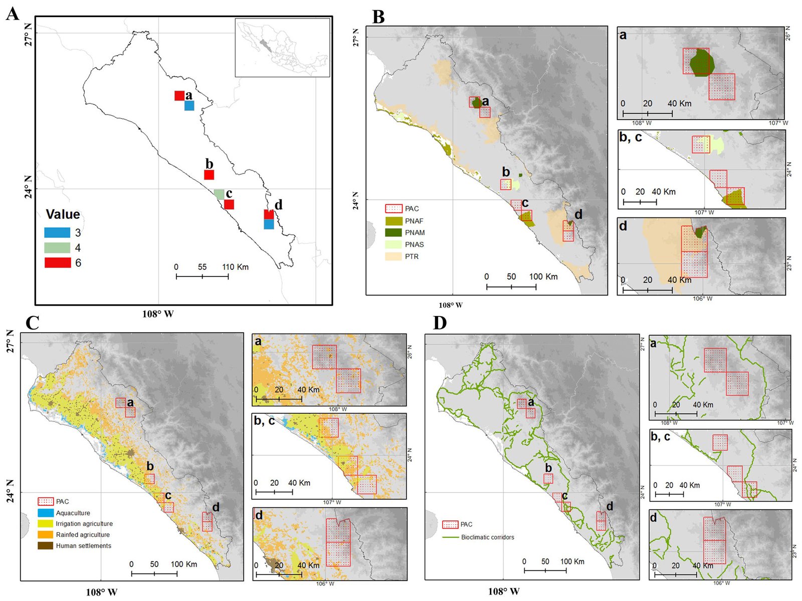
Figure 5. Consensus priority conservation areas (PAC) in the state of Sinaloa (A-D). Consensus map (A) superimposed to: Protected Natural Areas/Priority Terrestrial Regions (B), land use (C), and bioclimatic corridors (D). Categories of Protected Natural Areas: PNAS = state; PNAM = municipal; PNAF = federal; PTR = Priority Terrestrial Regions.
The addition of the ethnobotanical attributes to the protection status and richness of endemic species (SR+E+R) (Fig. 4D) showed an increase in the values for the areas from the Meseta de Cacaxtla (region 6, Fig. 1) to Sierra de Tacuichamona, but a decrease in the zones of the SMO. Adding the Priority Conservation Index to the richness (SR+PCI) (Fig. 4E) showed an increase and homogenization of the priority in all of the aforementioned regions, while adding protection status (SR+PCI+R) (Fig. 3F) did not significantly modify the areas of importance.
Finally, when considering only the ethnobotanical value plus the protection status (E+R), without considering species richness (i.e., eliminating the species that did not have those attributes), the zone of highest priority was concentrated nearly exclusively in the southern part of the state, within and adjacent to the Meseta de Cacaxtla (Fig. 3G). When considering PCI only or PCI plus risk category, there was again a homogenization of the high priority for the 2 mountainous areas (Surutato and Concordia), Meseta de Cacaxtla, Tacuichamona, and surrounding areas (Fig. 4H, I).
The priority conservation areas, as defined by the consensus among the 9 maps analyzed, were composed of 7 polygons grouped into 3 categories (Fig. 5): 4 cells with a value of 6 (of the maximum possible score of 9) in the northern part of the Sierra de Concordia, northwestern part of Sierra Surutato, Meseta de Cacaxtla, and Sierra de Tacuichamona; 1 with a value of 4 in the area between the Meseta de Cacaxtla and Tacuichamona; and 2 with a value of 3 in the southern part of the Sierra de Concordia and southeastern part of the Sierra de Surutato (Fig. 5A). However, since the 3 areas with a value of 3 or 4 were contiguous with areas with a value of 6, 4 priority conservation areas were proposed: Sierra de Surutato (Fig. 45-a), Sierra de Tacuichamona (Fig. 5A-b), Meseta de Cacaxtla (Fig. 5A-c), and Sierra de Concordia (Fig. 5A-d).
Superimposing the consensus map with the map of existing Protected Natural Areas (Fig. 5B) showed that these 4 consensus areas fall partially within protected areas: 1 federal (Área de Protección de Flora y Fauna Meseta de Cacaxtla, Fig. 5B-c), 1 state (Sierra de Tacuichamona, Fig. 5B-b), and 2 municipal (Reserva Chara Pinta in the Sierra de Concordia and Reserva de Surutato, Fig. 5B-d, B-a, respectively). The Sierra de Concordia also includes part of the terrestrial priority region Río Presidio. Regarding land use, the 2 consensus areas in the SMO were found in mixed pine-oak forest with low impact of agricultural activity (Fig. 5C-a, C-d), while the other 2, located in the Sinaloa and Sonora Hills and Canyons with Xeric Shrub and Low Tropical Deciduous Forest ecoregion, present moderate to high impact from irrigated and rainfed agriculture (Fig. 5C-b, C-c). When considering biological corridors, only the priority area in the Meseta de Cacaxtla overlapped with a bioclimatic corridor.
Discussion
The analyses of richness of endemic species and WE showed higher conservation priority in areas that were previously identified as having high endemism (Pío-León et al., 2023), low anthropogenic impact from agriculture, and which have also historically been subject to concentrated collection efforts (Sierra de Surutato and Sierra de Concordia) (Ávila-González et al., 2019; Gentry 1946; Vega-Aviña et al., 2021). On the other hand, the regions defined based on CWE reflected a high number of species known from a single locality, which could indicate the presence of small islands of endemism in the state or low collection effort. In contrast, the inclusion of the ethnobotanical criteria and protection status (E+R) shows a different pattern from species richness, concentrating high priority scored in an area of transition between the coastal plain of Sinaloa and the hills of Sinaloa and Sonora, near the coast in the center-south of the state. These regions correspond to the transition and ecotone between low tropical deciduous forest and thorn forest, which are strongly impacted by anthropogenic activities (irrigated and rainfed agriculture), suggesting that the species with the highest ethnobotanical importance and with protected status (IUCN or NOM-053-SEMARNAT-2010) are found near human activities that require stronger conservation attention than those located in the high parts of the SMO, where the threats are less severe.
The priority conservation areas indicated by the consensus map (Fig. 5) include the regions with the highest richness of endemic species plus the areas with the highest number of species with biocultural importance. These consensus areas are practically the same as those that were assigned the highest priority values when considering only the Priority Conservation Index (PCI) for each species; as such, this index was the most robust single indicator for selecting priority conservation areas. This index combines ethnobotanical parameters such as species’ uses and economic value with ecological parameters such as their distribution, habit, and habitat. Thus, it covers a broad range of criteria that are useful for defining priority species or areas for conservation.
All the priority conservation areas defined by the consensus map (Fig. 5) except 1 included part of a Protected Area polygon, although only 1 was under federal jurisdiction (Meseta de Cacaxtla). The only cell that did not overlap with a Protected Natural Area was adjacent to the Meseta de Cacaxtla, and it was the cell with the largest area of agriculture. This area is important because it contains the 2 species with the highest ethnobotanical value (Ebenopsis caesalpinioides and Stenocereus martinezii), which are also found in a risk category according to the IUCN and NOM-053-SEMARNAT-2010. This area therefore urgently requires conservation and restoration activities, especially for E. caesalpinioides, whose distribution is limited to the area surrounding this cell (Pío-León et al., 2023). Specifically, we recommend avoiding the conversion from rainfed agriculture to technified irrigated agricultural activities, since these are generally more aggressive toward native vegetation. This area is also important because it is located at the transition between lowland deciduous forest and thorn forest of Sinaloa, which could reflect high endemism, in addition to potentially serving as part of the bioclimatic corridor connecting the 2 most important terrestrial ANPs in the state, Meseta de Cacaxtla (federal) and Sierra Tacuichamona (state).
In the present study, the incorporation of the species’ biocultural parameters modified the priority areas for conservation compared to the areas selected when considering only the richness of endemic species, weighted endemism, or corrected weighted endemism. Specifically, the richness analysis identified priority areas in the mountainous and high-diversity regions of Sinaloa, while the ethnobotanical and ecological factors incorporated zones near the coast that have higher anthropogenic impact. The Conservation Priority Index identified all of these priority regions; for this reason, we propose it as a complete and robust index for identifying priority conservation areas. At the state level, we recommend that conservation and restoration actions be implemented in the area of transition between the low tropical deciduous forest and thorn forest. This area simultaneously presents the highest impact of anthropogenic activities and harbors the most important Sinaloa endemic species in terms of biocultural value and protection status —the “pitaya de Sinaloa” (Stenocereus martinezii) and the “guampinola” or “frutilla” (Ebenopsis caesalpinioides). This area should be considered a priority for both conservation and restoration, which would not have been identified as a priority if only the richness of endemism or CWE had been analyzed.
Acknowledgements
The first author is grateful to the Consejo Nacional de Humanidades, Ciencia y Tecnología (Conahcyt) for the grant awarded as part of the Estancias Posdoctorales por México program (I1200/320/2022). We also thank Jorge David López Pérez for his suggestions on data analysis, and the two anonymous reviewers for their comments and suggestions that improved our manuscript.
References
Ávila-González, H., González-Gallegos, J. G., López-Enríquez, I. L., Ruacho-González, L., Rubio-Cardoza, J., & Castro-Castro, A. (2019). Inventario de las plantas vasculares y tipos de vegetación del Santuario El Palmito, Sinaloa, México. Botanical Sciences, 97, 789–820. https://doi.org/10.17129/botsci.2356
Bradshaw, C. J. A., Ehrlich, P. R., Beattie, A., Ceballos, G., Crist, E., Diamond, J. et al. (2021). Underestimating the challenges of avoiding a ghastly future. Frontiers in Conservation Sciences, 1, 615419. https://doi.org/10.3389/fcosc.2020.615419
Conabio (Comisión Nacional para el Conocimiento y Uso de la Biodiversidad). (2023a). México megadiverso. Comisión Nacional para el Conocimiento y Uso de la Biodiversidad, Ciudad de México. Retrieved 01 December, 2023 from: https://www.biodiversidad.gob.mx/pais/quees
Conabio (Comisión Nacional para el Conocimiento y Uso de la Biodiversidad). (2023b). Ecosistemas de México. Comisión Nacional para el Conocimiento y Uso de la Biodiversidad, Ciudad de México. Retrieved 01 December, 2023 from: https://www.biodiversidad.gob.mx/ecosistemas/ecosismex
Dhar, U., Rawal, R. S., & Upreti, J. (2000). Setting priorities for conservation of medicinal plants ––a case study in the Indian Himalaya. Biological Conservation, 95, 57–65. https://doi.org/10.1016/S0006-3207(00)00010-0
De Lucena, R. F., Lucena, C. M., Araújo, E. L., Alves, Â. G., & Albuquerque, U. P. D. (2013). Conservation priorities of useful plants from different techniques of collection and analysis of ethnobotanical data. Anais da Academia Brasileira de Ciências, 85,169–186. https://doi.org/10.1590/S0001-37652013005000013
Gentry, H. S. (1946). Notes on the vegetation of Sierra Surotato in northern Sinaloa. Bulletin of the Torrey Botanical Club, 73, 451–462. https://doi.org/10.2307/2481592
González-Abraham, C., Ezcurra, E., Garcillán, P. P., Ortega-Rubio, A., Kolb, M., & Bezaury Creel, J. E. (2015). The human footprint in Mexico: physical geography and historical legacies. Plos One, 10, e0121203. https://doi.org/
10.1371/journal.pone.0121203
Gutiérrez-Rodríguez, B. E., Vásquez-Cruz, M., & Sosa, V. (2022). Phylogenetic endemism of the orchids of Megamexico reveals complementary areas for conservation. Plant Diversity, 44, 351–359. https://doi.org/10.1016/j.pld.20
22.03.004
IUCN (International Union for Conservation of Nature). (2023). The IUCN Red List of Threatened Species. Version 2022-2. Retrieved 01 December, 2023 from: https://www.iucnredlist.org
INEGI (Instituto Nacional de Estadística, Geografía e Informática). (2023). Censo agropecuario 2022. Resultados definitivos Sinaloa. Retrieved 25 January, 2024 from: https://www.inegi.org.mx/
Laso-Bayas, J. C., See, L., Georgieva, I., Schepaschenko, D., Danylo, O., Dürauer, M. et al. (2022). Drivers of tropical forest loss between 2008 and 2019. Scientific Data, 9, 1–8. https://doi.org/10.22022/nodes/06-2021.122
Laffan, S. W., & Crisp, M. D (2003) Assessing endemism at multiple spatial scales, with an example from the Australian vascular flora. Journal of Biogeography, 30, 511–520. https://doi.org/10.1046/j.1365-2699.2003.00875.x
Laffan, S.W., Lubarsky, E., & Rosauer, A. F. (2010) Biodiverse, a tool for the spatial analysis of biological and related diversity. Ecography, 33, 643–647. https://doi.org/10.1111/
j.1600-0587.2010.06237.x
Maassoumi, A. A., & Ashouri, P. (2022). The hotspots and conservation gaps of the mega genus Astragalus (Fabaceae) in the Old-World. Biodiversity and Conservation, 31, 2119–2139. https://doi.org/10.1007/s10531-022-02429-2
Mehta, P., Bisht, K., Sekar, K. C., & Tewari, A. (2023). Mapping biodiversity conservation priorities for threatened plants of Indian Himalayan Region. Biodiversity and Conservation, 32, 2263–2299. https://doi.org/10.1007/s10531-023-02604-z
Mora, F. (2019). The use of ecological integrity indicators within the natural capital index framework: The ecological and economic value of the remnant natural capital of México. Journal for Nature Conservation, 47, 72–92. https://doi.org/10.1016/j.jnc.2018.11.007
Murillo-Pérez, G., Rodríguez, A., Sánchez-Carbajal, D., Ruiz-Sánchez, E., Carrillo-Reyes, P., & Munguía-Lino, G. (2022). Spatial distribution of species richness and endemism of Solanum (Solanaceae) in Mexico. Phytotaxa, 558, 147–177. https://doi.org/10.11646/phytotaxa.558.2.1
Oyala, V. (2020). Sistemas de Información Geográfica. Retrie-
ved on December 25th, 2024 from: http://volaya.es/writing
Pío-León, J. F., González-Elizondo, M., Vega-Aviña, R., González-Elizondo, M. S., González-Gallegos, J. G., Salomón-Montijo, B. et al. (2023). Las plantas vasculares endémicas del estado de Sinaloa, México. Botanical Sciences, 101, 243–269. https://doi.org/10.17129/botsci.3076
QGIS Development Team (2019) Geographic Information System, version 3.4.8. QGIS Association. Retrieved 11 December, 2019 from: http://www.qgis.org
Qin, F., Xue, T., Yang, X., Zhang, W., Wu, J., Huang, Y. et al. (2022). Conservation status of threatened land plants in China and priority sites for better conservation targets: distribution patterns and conservation gap analysis. Biodiversity and Conservation, 31, 2063–2082. https://doi.org/10.1007/s10531-022-02414-9
Raven, P. H. (2018). Saving plants, saving ourselves. Plants People Planet, 1, 8–13. https://doi.org/10.1002/ppp3.3
Semarnat (Secretaría de Medio Ambiente y Recursos Naturales). (2019). Norma Oficial Mexicana NOM-059-SEMARNAT-2010. Protección ambiental-Especies nativas de México de flora y fauna silvestres-Categorías de riesgo y especificaciones para su inclusión, exclusión o cambio-Lista de especies en riesgo. Diario Oficial de la Federación, Ciudad de México. Retrieved 01 December, 2023 from: https://www.dof.gob.mx/nota_detalle.php?codigo=5578808&fecha=14/11/2019#gsc.tab=0
Sosa, V., & De-Nova, J. (2012). Endemic angiosperm lineages in Mexico: hotspots for conservation. Acta Botanica Mexicana, 100, 293–315. https://doi.org/10.21829/abm100.2012.38
Ulloa-Ulloa, C., Acevedo-Rodríguez, P., Beck, S., Belgrano, M. J., Bernal, R., Berry, P. E. et al. (2017). An integrated assessment of the vascular plant species of the Americas. Science, 358, 1614–1617. https://doi.org/10.1126/science.aao
0398
Vargas-Amado, G., Castro-Castro, A., Harker, M., Vargas-Amado, M. E., Villaseñor, J. L., Ortiz, E. et al. (2020). Western Mexico is a priority area for the conservation of Cosmos (Coreopsideae, Asteraceae), based on richness and track analysis. Biodiversity and Conservation, 29, 545–569. https://doi.org/10.1007/s10531-019-01898-2
Vega-Aviña, R., Vega-López, I. F., & Delgado-Vargas, F. (2021). Flora nativa y naturalizada de Sinaloa. Culiacán, Sinaloa: Universidad Autónoma de Sinaloa.
Villaseñor, J. L., & Meave, J. A. (2012). Floristics in Mexico today: insights into a better understanding of biodiversity in a megadiverse country. Botanical Sciences, 100, S14–S33. https://doi.org/10.17129/botsci.3050
Villaseñor, J. L., Ortiz, E., & Hernández-Flores, M. M. (2022). The vascular plant species endemic or nearly endemic to Puebla, Mexico. Botanical Sciences, 101, 1207–1221. https://doi.org/10.17129/botsci.3299
Wiken, E., Jiménez-Nava, F., & Griffith, G. (2011). North American Terrestrial Ecoregions-Level III. Montreal, Canada: Commission for Environmental Cooperation. Retrieved Jul 17, 2021 from: http://www3.cec.org/islando
ra/en/item/10415-north-american-terrestrial-ecoregionsle
vel-iii

Mitogenome of the Golden Eagle (Aquila chrysaetos) in northwestern Baja California, Mexico: phylogenetic relationships and genetic variation
Francisco J. García-De León a, Gorgonio Ruiz-Campos b, *, Jesús Roberto Oyervides-Figueroa c, Gonzalo De León-Girón b, Carlos Alberto Flores-López b, Dante Magdaleno-Moncayo d, Alicia Abadía-Cardoso e
a Centro de Investigaciones Biológicas del Noroeste, S.C., Laboratorio de Genética para la Conservación, Av. Instituto Politécnico Nacional 195, Playa Palo de Santa Rita Sur, 23096 La Paz, Baja California Sur, Mexico
b Universidad Autónoma de Baja California, Facultad de Ciencias, Carretera Ensenada-Tijuana Km. 103 s/n, 22860 Ensenada, Baja California, Mexico
c Centro de Investigación Científica y de Educación Superior de Ensenada, Departamento de Acuicultura, Carretera Tijuana -Ensenada 3918, Zona Playitas, 22860 Ensenada, B.C., Mexico
d Universidad Autónoma de Baja California, Facultad de Ingeniería, Arquitectura y Diseño, Carretera Ensenada-Tijuana Km. 103 s/n, 22860 Ensenada, Baja California, Mexico
e Universidad Autónoma de Baja California, Facultad de Ciencias Marinas, Carretera Ensenada-Tijuana Km. 103 s/n, 22860 Ensenada, Baja California, Mexico
*Corresponding author: gruiz@uabc.edu.mx (G. Ruiz-Campos)
Received: 20 August 2024; accepted: 20 February 2025
Abstract
We assembled and annotated the mitochondrial genome of golden eagles from the northwest of Baja California, Mexico, using reference and de novo strategies to analyze the synteny of mitochondrial genes, the phylogenetic relationships, and genetic variation of mitochondrial DNA. The length of the Golden Eagle mitogenome was 17,472 bp (base pairs) with a base composition of A (29.8%), C (32.5%), G (14.0%), and T (23.6%). The mitogenome contains 13 genes coding for the protein complexes coxI II-III, Cytb, cATP 6 and 8, and Nicotinamide Adenine Dinucleotide (NADH 1-6); this arrangement is consistent with the general model of the mitogenome reported in other congeneric members. Mitogenomes of individuals from northwestern Baja California are unique and they differ from the mitogenome of southern California golden eagles in 3 traits: 1) molecule size is 140 bp larger than that previously reported, 2) the addition in the annotation of a region called pseudo control (ψRC), and 3) the annotation in 2 fractions of the coding region for the protein NADH dehydrogenase subunit 3 (ND3). The genetic diversity and phylogenetic analyses of the individual genes and mitogenome support a close genetic relatedness between the golden eagles from northwestern Baja California and southern California region.
Keywords: Mediterranean region; Mitochondrial lineages; Mitochondrial genome; Next generation sequencing; Non-model species
Mitogenoma de águila real (Aquila chrysaetos) en el noroeste de Baja California, México: relaciones filogenéticas y variación genética
Resumen
Ensamblamos y anotamos el genoma mitocondrial del águila real del noroeste de Baja California, México, utilizando estrategias de referencia y de novo para analizar la sintenia de genes mitocondriales, las relaciones filogenéticas y la variación genética del DNA mitocondrial. La longitud del mitogenoma fue 17,472 pb (pares de bases) con una composición de bases de A (29.8%), C (32.5%), G (14.0%) y T (23.6%). El mitogenoma contiene 13 genes codificantes de los complejos proteínicos coxI II-III, Cytb, cATP 6 y 8, y nicotinamida adenina dinucleótido (NADH 1-6); esto fue consistente con el modelo general del mitogenoma reportado en otros congéneres. Los mitogenomas de individuos del noroeste de Baja California son únicos y se diferencian del mitogenoma de individuos del sur de California en 3 rasgos: 1) el tamaño de molécula es 140 pb más grande que el reportado, 2) adición de la región llamada pseudocontrol (ψRC) y 3) anotación en 2 fracciones de la región codificante de la proteína NADH deshidrogenasa subunidad 3 (ND3). La diversidad genética y los análisis filogenéticos de los genes individuales y el mitogenoma respaldan una estrecha relación genética entre las águilas reales del noroeste de Baja California y la región del sur de California.
Palabras clave: Región mediterránea; Linajes mitocondriales; Genoma mitocondrial; Secuenciación de próxima generación; Especies no modelo
Introduction
The Golden Eagle, Aquila chrysaetos, is an accipitrid of boreal distribution that inhabits a variety of open and semi-open biotopes from sea level to 3,630 m in altitude in biomes as tundra, chaparral, temperate grassland, temperate deciduous forest, and coniferous forest (De León-Girón et al., 2016; Flesch et al., 2020; Kochert et al., 2002; Watson et al., 2011). This emblematic species is known to occur in Mexico in the arid and semiarid environments of the northern and central regions, including some locations as south as Oaxaca (Bolger et al., 2014; De León-Girón et al., 2016; Howell & Webb, 1995; Rodríguez-Estrella, 2002; Rodríguez-Estrella et al., 1991, 2020). Although the demography of the Golden Eagle has been determined with different genetic methods that confirm the structuring of its populations (Craig et al., 2016; Doyle et al., 2016), little is known about the genetic identity of populations of this eagle in its distribution range. Northwestern Baja California is considered the greatest nesting and conservation potential region for the Golden Eagle in Mexico (De León-Girón et al., 2016; Rodríguez-Estrella, 2002; Rodríguez-Estrella et al., 1991; Tracey et al., 2017), with vast areas of habitats still pristine for the population conservation of this species shared with the United States of America (Craig et al., 2016; De León-Girón et al., 2016, 2024; Doyle et al., 2014; Katzner et al., 2023).
Studies based on mitochondrial DNA (mtDNA) allow determining the current state of conservation of species, as well as the identification of significant evolutionary and management units with their demographic aspects (Moritz, 1994). With the advent of next-generation sequencing (NGS) technologies (especially on complete mitochondrial genomes), new studies with non-model species became more common. As was the case for various species of the family Accipitridae, including the Golden Eagle. Doyle et al. (2014) were the first to describe the nuclear and mitochondrial genome of the Golden Eagle from the central California region, in the USA.
In this study we focus on the synteny of mitochondrial genes, the phylogenetic relationships, and the mitochondrial genetic diversity among Golden Eagle individuals in northwestern Baja California, Mexico. Given the high migration potential of this species, individuals collected in northwestern Baja California are predicted to be phylogenetically related to the westernmost Golden Eagle population in the USA. Therefore, studies focused on examining the genetic variation at the mitochondrial level will allow better decision-making for management and conservation programs for the species in a binational spectrum. In the same way, our study will be a valuable reference for analyzing other Golden Eagle populations in Mexico and other regions of its distribution range.
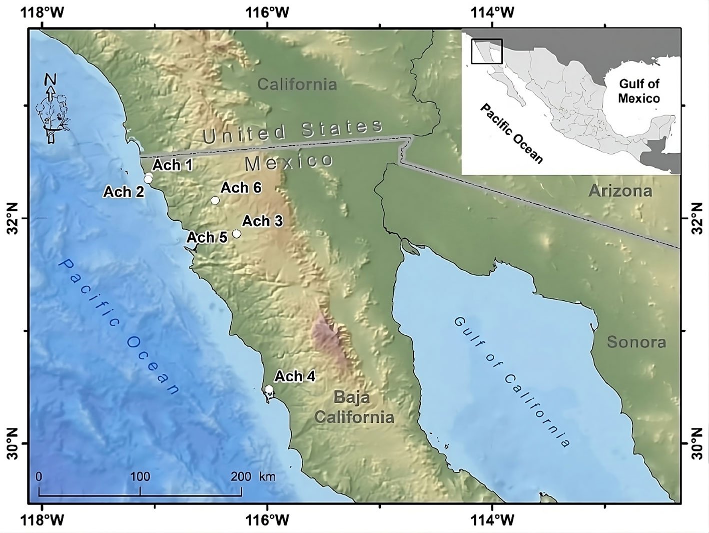
Figure 1. Geographical location of the Golden Eagle voucher specimens examined for mitogenome in the northwestern Baja California, Mexico. Geographic coordinates for each individual can be found in Supplementary material T1. Map by Rafael Hernández Guzmán.
Materials and methods
Tissue samples of 6 Golden Eagle specimens from northwestern Baja California, Mexico were obtained. These specimens were found dead in different agriculture valleys of the Mediterranean region in northwestern Baja California, Mexico, between the municipalities of Rosarito and San Quintín, from 1995 to 2014, and deposited as vouchers in the Bird Collection of the Science Faculty, at the Autonomous University of Baja California (UABC), campus Ensenada (Fig. 1, Supplementary material: T1).
For the DNA extraction, tissue samples of the pads of the feet of 5 Golden Eagle specimens referred to here as Ach 1 to Ach 5 were obtained. DNA using the nucleic acid purification method by differential saline precipitation (Aljanabi & Martinez, 1997) was extracted. Both feathers and blood for the Ach 6 sample (Supplementary material: T1) were used and extracted DNA with the Qiagen Blood & Tissue kit. The quality and quantity of the extracted DNA in both cases was evaluated using Nanodrop, Qubit and agarose gel electrophoresis.
Extracted DNA (from 77 to 210 ng/µL per sample quantified in Nanodrop for Ach1-Ach5 individuals and 0.581 ng/µL for Ach6 quantified in Qubit) was purified with SpeedBeads magnetic beads (Thermo-Scientific, Waltham, MA, USA) at a 1.2:1 beads:DNA ratio and resuspended in 50 µl of TLE1X buffer. Libraries for shotgun sequencing were prepared, for which purified DNA from each individual was fragmented by sonication in a Bioruptor® (Diagenode, Liege, Belgium) using 2 rounds, each consisting of 5 cycles of 30 sec of sonication and 30 sec without sonication at the highest setting. DNA fragments were then prepared using the Kapa Biosystems® Hyper Prep Kit (KR0961–v4.15, Roche, Basel, Switzerland), with which end repair and A-tailing were performed, adapters were ligated, and PCR was performed with indexed primers (Glenn et al., 2020) for 14 cycles. Following amplification, fragment size selection was performed by double-dip with SpeedBeads magnetic beads (Thermo-Scientific, Waltham, MA, USA) that allow to preserve fragments between ~250 and ~700 base pairs (bp) for each of the samples, which are the appropriate insert size for the Illumina platform. Sequencing was performed paired end on 2 different platforms. We sequenced the Ach1-Ach5 samples on the Illumina MiSeq V.3 at the Georgia Genomics and Bioinformatics Core (GGBC) to generate 300-bp paired-end fragments, and we sequenced Ach6 on an Illumina HiSeq 4000 at the Oklahoma Medical Research Foundation Clinical Genomics Center to generate 150-bp paired-end fragments.
Bioinformatic analysis. The quality of the raw sequences was evaluated using the FastQC program (Andrews, 2010). Subsequently, the sequences using a standard treatment were filtered using the Trimmomatic software (Bolger et al., 2014) with 4 steps. In the first step, the sequencing adapters and over-represented sequences were removed by means of the ILLUMINACLIP function. The second step discarded sequences with a quality value below 30 QS with the AVGQUAL function. The third step removed fragments below 25 QS with the SLIDINGWINDOW function. The fourth step did an even stricter cleanup using MAXINFO. This step conserved sequences of at least 100 base pairs and was configured to preferentially conserve longer sequences with a value of 0.3. For the Ach 5 specimen, an extended and modified version of the standard treatment was used due to the low quality of sequences. This involved applying the SLIDINGWINDOW function, which modifies the quality value.
Assembly and annotation. Two strategies were followed to assemble the mitochondrial genomes: the reference based and the de novo strategy (Machado et al., 2015, 2018). Mapping against a reference mtDNA genome was performed using the Bowtie2 program version 2.3.4.2 with clean reads (Langmead & Salzberg, 2012). The reference mitochondrial genome was from the same species A. chrysaetos, with the GenBank accession number of KF905228.1. De novo assembly only for samples Ach 2 to Ach 6 was performed using the A5-miseq pipeline (Coil et al., 2015). Due to the large number of reads after the filter (Supplementary material: T2) sample Ach 1 was analyzed with the Velvet software version 1.1 (Zerbino & Birney, 2008). The mitogenome was annotated from the scaffolds obtained from the de novo assemblies. We determined scaffolds longer than 4 Kpb by applying a search with the BLAST tool (Basic Local Alignment Search Tool) of the NCBI (National Center for Biotechnology Information) website. The scaffolds were aligned to achieve greater coverage considering the length of the reference genome used previously. Afterwards, RNAweasel (http://megasun.bch.umontreal.ca/RNAweasel/) was implemented to the identification of tRNA’s (transfer RNA), rRNA’s (ribosomal RNA) and introns and, in turn, MFannot (http://megasun.bch.umontreal.ca/RNAweasel/) for the identification of proteins and open reading frames (Sieber et al., 2018).
In addition to the previous annotation, MITOS web server (Bernt et al., 2013) was used to assist in the annotation of de novo mitochondrial genomes, allowing gene names, tRNA and rRNA secondary structures, and codon usage to be obtained. Finally, a manual curation of the annotations was used to review the 6 existing reading frames with the UGENE software (Okonechnikov et al., 2012). The control region was identified based on 99% similarity with an A. chrysaetos partial control region sequence (EF459579.1). Genome Vx software (Conant and Wolfe, 2008) was used to map the Golden Eagle’s mitogenome, using individual Ach 6 to achieve this analysis.
In the annotation of the de novo assembly, the ND3 protein appeared divided into 2 fractions (see Results), a trait that was not reported by Doyle et al. (2014). Therefore, an experimental verification was required through PCR amplification and its subsequent Sanger sequencing. We designed primers from de novo assembly using the NCBI Primer-BLAST program: ND3Ach-1 (5’GCCTGATACTGGCACTTCGT3’ and 5’CCCTATCAATCTGACCCACCG3’) which generates a 716 bp fragment and ND3Ach-2 (5’CTTCTTCGTCGCTACAGGCT3’ and 5’CCTTCCACCGAACCCACTTAA3’) which generates a 774 bp fragment. Eight Golden Eagle samples from the Ornithological Collection of the Faculty of Sciences of the Autonomous University of Baja California were used for PCR amplification. These samples correspond to the 6 individuals used for sequencing and 2 extra samples that are not part of the mitogenome assembly study. The conditions of the PCR reaction were as follows: 6 min at 94°C, 35 cycles of denaturation, annealing, and extension at 94°C for 30 sec, 51°C for 30 sec and at 72°C for 1.5 min, respectively. A final elongation stage at 70°C for 7 min, and a final conservation stage at 15°C. We sent the amplified fragments for sequencing to the SeqXcel.inc Company in San Diego, California, and analyzed with the ABI PRISM® 3130xl Genetic Analyzer DNA kit.
Synteny and search for polymorphisms. A posteriori synteny analysis was performed between the Golden Eagle mitogenome reported by Doyle et al. (2014) and the newly assembled mitochondrial genome of this study. This analysis was carried out with the MAUVE software (Darling et al., 2004). The same reference mitogenome was used to call SNP’s and INDEL’s for the 6 genomes assembled in this work using the SAMtools program (Li, 2011). Filtering the call quality of the variants involved discarding those with a value less than 20 Qs and keeping those with at least 5X depth (Li, 2011). Each variant was manually evaluated, retaining SNPs and INDELs where at least half of the aligned reads showed the change and verified its existence in at least one other individual (Fridjonsson et al., 2011).
Phylogenetic relationships. Phylogenetic relationships were inferred using the individual gene dataset and the mitogenome. The individual gene fragments analyzed consisted of the ND2, ND3, coxI and Cytb recovered from Aquila chrysaetos individuals from GenBank (Supplementary material: T3) and those produced in this study. The mitogenome analysis for phylogenetic relationships consisted of 10 complete mitogenomes: 6 obtained in this study, 2 reference samples of Aquila chrysaetos (LR822062 from the United Kingdom and NC_024087.1 from California, USA), 1 reference sample classified as Aquila heliaca (NC_035806.1), but has been reported to actually consist of a A. chrsyasetos individual (Sangster & Lukesenburg, 2021) and 1 outgroup (Aquila nipalensis, GenBank accession number NC_045042.1). Both datasets were aligned using the MAFFT 7 algorithm (Katoh & Standley, 2013). Removing the non-conserved regions between the sequences of the multiple alignments was done using the online program Gblocks with the default parameters (Castresana, 2000). The nucleotide substitution model and the mutation rate were determined using JModelTest (Posada, 2008), considering the Bayesian information criterion (BIC).
Two phylogenetic reconstruction methods were used: Maximum Likelihood (ML) and Bayesian analysis. In IQ-TREE (Nguyen et al., 2015) the ML method (Felsenstein, 1981) was run with the DNA substitution model selected by ModelFinder (Kalyaanamoorthy et al., 2017) and 1,000 bootstrap pseudo replicates were performed (Hoang et al., 2017). Bayesian inference was used with MrBayes program (Ronquist et al., 2012); for this, 4 Markov Monte Carlo chains (MCMC) were implemented with a total of 10 million generations, and a sampling every 1,000 generations. To construct the consensus phylogenetic tree, a 25% of burn-in was applied. The support of the nodes was evaluated via the posterior probability values. The results of both approaches were visualized with FigTree 1.4 (Rambaut, 2009). For the mitogenome phylogenetic tree, the dataset on genes that were annotated across the entire mitogenome were partitioned (Supplementary material: T4). To determine the most appropriate DNA substitution model for each gene, the Akaike Information Criterion test implemented in jModelTest2 (Darriba et al., 2012; Guindon & Gascuel, 2003) was used (see selected models for each gene in Supplementary material: T4). The partitioned mitogenome dataset was used to estimate a Bayesian phylogenetic tree in MrBayes (Ronquist et al., 2012). The Bayesian analysis was carried out by running 4 MCMC chains for 5 million generations and saving the trees every 1,000 generations. The consensus phylogenetic tree was constructed using a 10% burn-in.
Genetic diversity. Individual DNA segments from the coxI, Cytb, ND2, and -ND3 genes were used to estimate the genetic diversity parameters for the A. chrysaetos species complex since these were the genes that had a relative amount of A. chrysaetos DNA sequences available in GenBank. Using DNA sequences from the Baja California individuals produced in this study and reference sequences from the species complex (Supplementary material: T3) the following indices were estimated with DnaSP 6 (Rozas et al., 2017): the number of segregating sites (S), number of haplotypes (Nh), haplotype diversity (Hd), and nucleotide diversity (π). Genetic diversity indices were calculated among all sequences included in the respective datasets and within specific groups of sequences according to phylogenetic clades or geographic origin of samples. In addition, the genetic distance (uncorrected p-distance) between and within the phylogenetic clades observed within the mitochondrial genetic lineages in PAUP software was estimated (Swofford, 1993). The clade OTU1 included sequences from a diverse geographical background, including all the DNA sequences of the Baja California golden eagles. In contrast, the A. chrysaetos DNA sequences grouped in the other closely related clade were classified as OTU2. Additionally, the DNA sequence of an individual of A. chrysaetos from California (Southern Sierra Nevada) was analyzed separately to compare its genetic distance with those from Baja California, given the geographical proximity between both populations.
Results
Raw sequencing reads ranged from 3,324,579 (individual Ach 1) to 539,825 (individual Ach 4). The number of total sequences after the filter ranged between 3,251,746 (Ach 1) and 526,875 (Ach4) (Supplementary material: T2A).
Assembly and annotation. There were large differences in assembly between individuals; for example, the average depth in the reference mapping for individual Ach 1 is 30.5X, while for Ach 6 is 168.3X, even though Ach 6 had fewer total reads than Ach 1. Assemblies for individuals Ach 1-5 showed fewer aligned sequences (Supplementary material: T2A). For de novo assembly, the average depth for individual Ach 6 is 8.0X. The longest scaffold generated (17,472 bp) allowed us to assemble the entire mitogenome of the Ach 6 individual, eliminating the need to align multiple scaffolds to recover the full length (Supplementary material: T2B). The data yield was inferior when doing de novo assembly for Ach 1-5 individuals, and none of these individuals allowed the recovery of the complete mitochondrial genome (Supplementary material: T3B).
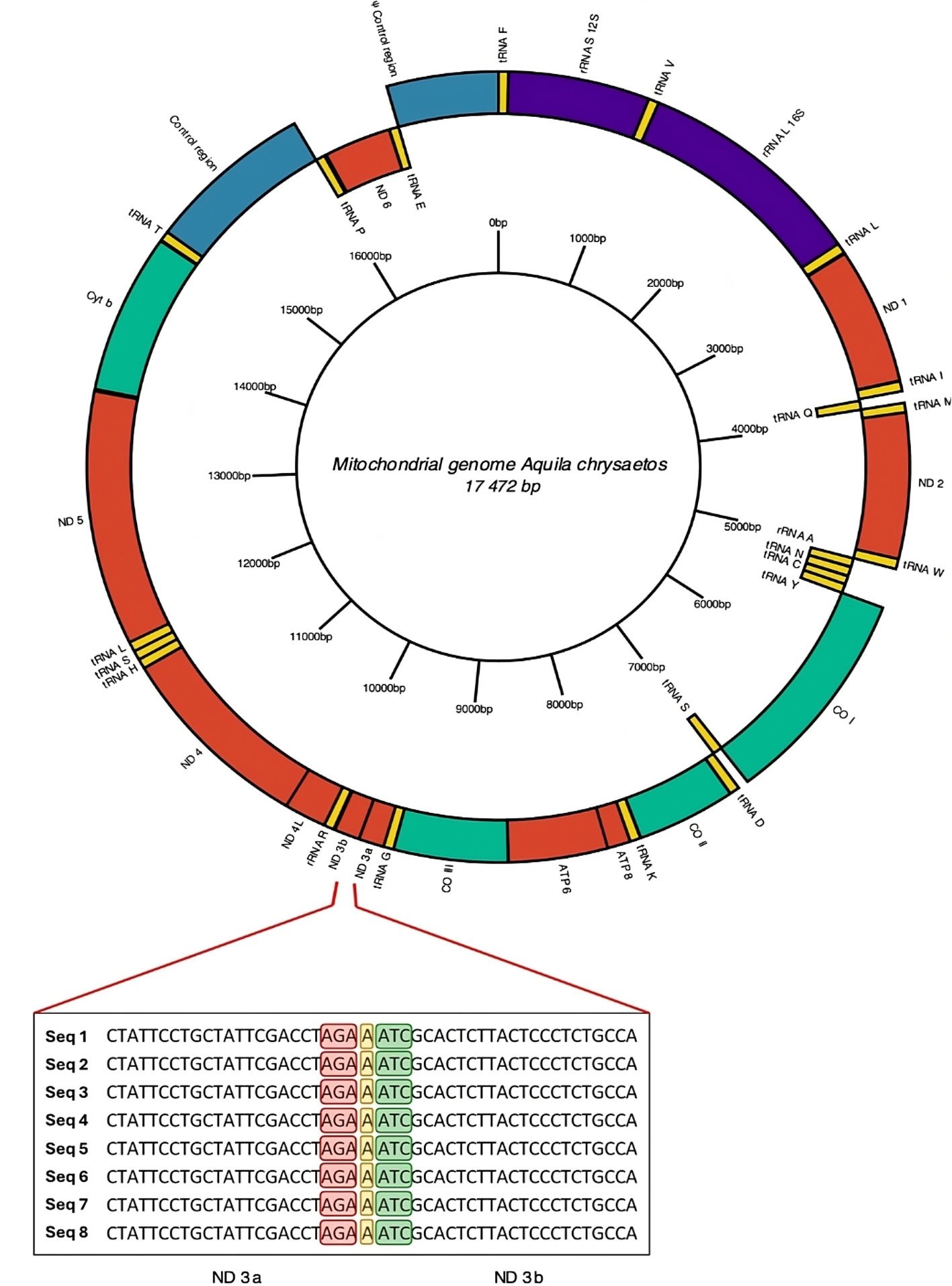
Figure 2. Mitogenome annotated by de novo assembly for Golden Eagle (Ach6) from Baja California, Mexico. In the central part of the diagram in a ring form is shown a scale of the length of mitochondrial genome clockwise. Enlarged view of the section showing the division into 2 fractions of the mitochondrial gene for NADH dehydrogenase subunit 3 (ND3). The stop codon of the ND3a fraction is highlighted in red, the insertion of nucleotide A in yellow, and the start codon of the ND3b fraction in green. The ND3 gene is composed entirely of 352 bp; the ND3a fraction is 207 bp long, while the ND3b fraction is 144 bp long.
Based on the above results, we annotated and curated the mitochondrial genome using only the complete mitogenome obtained by de novo assembly of the Ach 6 individual. All 3 annotation tools identified tRNAs, and none of the tools identified introns within the sequence. The MITOS program (Fig. 2, Supplementary material: T4) was the only software that identified all the genetic elements, such as the 22 tRNAs, 2 rRNAs, and the 13 protein-coding genes that make up the mitogenome. This last annotation was the most complete, so the curation was made from it. We found a region with 7 nucleotide bases that is composed of an AGA stop codon of the ND3 protein, followed by an adenine (A) and finally an ATC start codon that codes for isoleucine. This region divides the ND3 fragment into the 2 regions proposed here (ND3a and ND3b, Fig. 2).
Synteny and search for polymorphisms. The linear order of the mitogenome of Ach 6 coincides with the reference genome (Accession number MT319112.1, Supplementary material: T5). We consider the SNPs and INDELs identified in the Ach 6 reliable, given that the average coverage is 168.3X, and their call quality was high (Supplementary material: T2A). Most SNPs and INDELs are found within genes that code for some protein, transfer RNA and ribosomal genes. The coxI gene presented the greatest number of SNPs with respect to the reference genome in the 6 individuals, while the Cytb and tRNA F genes presented the greatest length changes in the INDELs. In addition, in the ND3 gene, there is a consistent change in the sequences of the 6 individuals with respect to the reference genome (Table 1).
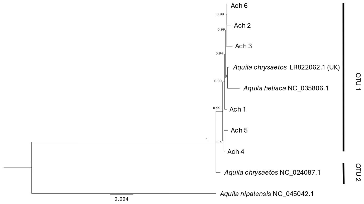
Figure 3. Bayesian phylogenetic tree based on the mitogenome for Golden Eagle voucher specimens from northwestern Baja California, Mexico. Posterior probabilities are shown above internal nodes. GenBank accession numbers are positioned next to reference sequences. Aquila nipalensis was used as an outgroup for rooting the tree. Two Operational Taxonomic Units are identified (OTU 1, 2).
Phylogenetic relationships. With the use of the mitogenome we constructed a phylogenetic tree that identified 2 clades with strong support (1): OTU1 that includes all the individuals analyzed in this study, plus 2 GenBank sequences (Aquila chryseatos, LR82062.1 from the United Kingdom and A. heliatica, NC_035806.1), and OTU2 that corresponds to a GenBank sequence of a specimen collected in California (Fig. 3). For their part, the phylogenetic trees obtained with the fragments of individual genes (ND2, ND3, Cytb and coxI) did not resolve the divergence between individuals from Baja California and California obtained with the mitogenome, but all except the ND3 gene showed a divergence (OTUs 1 and 2), mainly with respect to eagles from the European continent (when information on the collection location is reported, Supplementary material: F1).
Genetic diversity. We observed low genetic diversity, for instance, ND3, ND2, and coxI each had a single segregating site (Table 2), resulting in low nucleotide diversity values (0.0005, 0.0008, and 0.0002, respectively). In contrast, Cytb was the most polymorphic, with a total of 10 segregating sites and a nucleotide diversity an order of magnitude larger (0.00297) (Table 2). The genetic diversity found within OTU1 was higher than that found in OTU2 (Table 2), although OTU1 was not a geographically homogeneous clade among the trees of the different mitochondrial genes, for example in the case of ND2 it was made up of North American eagles, including the individuals of this study, but coxI apart from the previous ones was constituted with eagles from Sweden, Norway and Japan (Table 2).
Discussion
Despite using 2 sequencing platforms for the mitogenome of Golden Eagle from northwestern Baja California, Mexico, we successfully assembled the mitochondrial genome of all 6 individuals by the reference method. This included some individuals (Ach 1-5) with non-consensus regions. Bolger et al. (2014) recommend a pre-processing step of the readings before any analysis, be it assembly by reference or de novo, and mention that if the library and identification adapters are not removed, they can be incorporated in the final assembly. In our case, the pre-processing of the sequences positively influenced the performance of both assemblies and the SNP’s call since the quality of the sequence of the 6 individuals was considerably improved after pre-processing in all aspects of quality reporting.
Table 1
Location of SNP’s and INDEL’s in mitogenomes. Call of SNP’s and INDEL’s for each the Ach 1-6 specimens versus the reference genome of Golden Eagle from the southern Sierra Nevada in California, USA (GenBank accession: KF905228). Pos: Mitogenome position; Ref: nucleotide present in reference sequence. ψCR: Mitochondrial pseudogene control region.
| Pos. | Ref. | Ach1 | Ach2 | Ach3 | Ach4 | Ach5 | Ach6 | Gen |
| SNP’s | ||||||||
| 1,505 | G | A | A | A | ||||
| D-loop | ||||||||
| 1,515 | T | C | ||||||
| 3,130 | G | A | A | A | ||||
| 3,566 | A | G | ND6 | |||||
| 3,695 | T | A | A | A | ||||
| 3,696 | T | A | A | A | ||||
| 5,557 | G | A | A | A | A | A | LSU rRNA | |
| 6,646 | G | A | A | A | ND1 | |||
| 7,141 | A | G | ||||||
| 8,269 | C | T | A | T | ND2 | |||
| 8,593 | A | G | G | A | G | |||
| 8,723 | G | A | A | A | A | tRNA-Trp | ||
| 10,925 | C | T | T | T | T | T | ||
| 10,963 | T | C | ||||||
| 10,970 | C | T | T | T | T | T | ||
| 10,975 | T | C | coxII | |||||
| 11,003 | A | G | G | |||||
| 11,011 | C | T | ||||||
| 11,205 | A | G | ||||||
| 11,213 | C | T | ||||||
| 11,237 | C | T | ||||||
| 11,282 | G | A | ||||||
| 11,284 | G | T | ||||||
| 11,285 | A | C | ||||||
| 11,351 | T | C | ||||||
| 11,354 | A | G | ||||||
| 11,378 | C | T | T | |||||
| 11,432 | C | T | T | T | T | T | ||
| 11,489 | A | C | C | C | C | C | C | |
| 11,493 | T | T | tRNA-Lys | |||||
| 11,496 | G | A | ||||||
| 11,505 | T | G | ||||||
| 17,278 | G | A | A | ND5 | ||||
| INDEL’s | ||||||||
| Table 1. Continued | ||||||||
| Pos. | Ref. | Ach1 | Ach2 | Ach3 | Ach4 | Ach5 | Ach6 | Gen |
| 3 | CTAA | CTAA CTTC CAAA CTAA | Cyt b | |||||
3,550 | T | TGTG AACA A | ψCR | |||||
| 3,701 | CAAA | CCCA CCAA TA | CCAA CAAT AT | tRNA-Phe | ||||
| 13,378 | T | TC | TC | TC | TC | TC | TC | ND3 |
Table 2
Genetic diversity and haplotype composition from gene segments. Tax Set: Group of sequences included in taxonomic set; N: number of sequences; bp: base pairs of DNA sequence included in alignment; S: number of segregating sites; Nh: number of haplotypes; Hd: haplotype diversity; Nd: nucleotide diversity; North America: sequences from either Canada or USA. All sequences from ND3 formed a single clade, and thus were analyzed as a single group. OTUs 1 and 2 in each individual gene refer to the clades detected in each phylogenetic analysis, see Supplementary material F1.
| Mitochondrial sequence | Tax Set | N | bp | S | Nh | Hd | Nd |
| ND3 | All | 11 | 352 | 1 | 2 | 0.182 | 0.00053 |
ND2 | OTU1 | 8 | 1,039 | 0 | 1 | 0 | 0 |
| OTU2 | 4 | 1,039 | 0 | 1 | 0 | 0 | |
| North America | 2 | 1,039 | 0 | 1 | 0 | 0 | |
| Europe | 3 | 1,039 | 0 | 1 | 0 | 0 | |
| All | 12 | 1,039 | 1 | 2 | 0.485 | 0.00087 | |
coxI | OTU1 | 13 | 1,551 | 1 | 2 | 0.154 | 0.00025 |
| OTU2 | 2 | 1,551 | 0 | 1 | 0 | 0 | |
| North America | 4 | 1,551 | 0 | 1 | 0 | 0 | |
| Europe | 4 | 1,551 | 1 | 2 | 0.5 | 0.00082 | |
| All | 15 | 1,551 | 1 | 2 | 0.133 | 0.00022 | |
Cytb | OTU1 | 13 | 1,143 | 1 | 2 | 0.154 | 0.00016 |
| OTU2 | 3 | 1,143 | 1 | 2 | 0.667 | 0.00069 | |
| North America | 4 | 1,143 | 1 | 2 | 0.5 | 0.00052 | |
| Europe | 5 | 1,143 | 9 | 3 | 0.02688 | 0.00541 | |
| All | 16 | 1,143 | 10 | 4 | 0.442 | 0.00297 |
The most reliable mitogenome assembly was that of Ach 6 individual due to its higher alignment rate, its greater depth, and its 100% coverage of the reference genome. This ensemble can be considered true and not an artifact due to the procedures used, such as sampling every 500 generations and a burn-in value of 600,000 generations (Lerner & Mindell, 2005). In addition, we analyzed the data with Bowtie2, which implements an alignment strategy based on the FM-Index and Burrows-Wheeler. These programs have been shown to work well for applications such as INDEL discovery (Lindner & Friedel, 2012) and for aligning long sections of the reference genome (Thankaswamy-Kosalai et al., 2017). Hunt et al. (2014) pointed out that the best result of assembling a genome de novo is when it is contained in a single scaffold for the entire mitochondrial DNA molecule or for each chromosome in the case of the nuclear genome. The Golden Eagle mitochondrial genome assembly of individual Ach 6 was the best because it was found within a single scaffold (17,472 bp) and its depth was at least 8.0X (Supplementary material: T2B; Baker, 2012).
The extension and position of the genes in the mitogenome of the Golden Eagle described in this study (Fig. 2, Supplementary material: T4) showed differences compared to those reported by Doyle et al. (2014) from an individual sampled in central California. For example, the size of the mitogenome described here is larger (17,472 bp) than the one reported by Doyle et al. (2014) (17,332 bp), with a difference of 140 bp. When experimentally analyzing the size of the ND3 gene amplified fragments, the size was between 700 and 800 bp, that is, the theoretically expected size. Another difference consisted in the fraction of the gene encoding the ND3 protein reported here as split into 2 segments (ND3a and ND3b). The distinction of the 2 subunits is, within the reading frame, a region made up of 7 nucleotides between the ATC start codon that starts the protein, and the TAA stop codon that marks the end of the protein. The first 3 of these 7, code for a new AGA stop codon, followed by an adenine (A) nucleotide and 3 nucleotides that code for a new ATC start codon. This causes 2 coding portions to coexist, annotated as ND3, separated by a single nucleotide that changes the reading frame, causing the second portion to appear with its start and stop codons. Mindell et al. (1998) report a nucleotide that is not translated within the ND3 protein sequence. Eberhard and Wright (2016) mentioned that such a trait is observed in the entire order Psittaciformes (parrots, parakeets, and allies).
Specifically, a variety of distinct indels have been found within several of the mitochondrial protein-coding genes in Psittaciformes (Eberhard & Wright, 2016), with variations in terms of their evolutionary origin since some are present in all Psittaciformes and some are more recent in origin and only found within specific taxa. Slack et al. (2003) reported variation in the length of the mitochondrial ND6 gene in other avian taxa. Overall, the biological implications of these variations remain unclear until more studies on the proteins are performed to determine if the protein compositions become altered by these variations. However, the experimental verification carried out in the present study strengthens our annotation as 2 fractions for the ND3 region of the A. chrysaetos mitogenome. Also, we noted the regulatory non-coding region (the pseudo control region, ψCR) to be highly conserved among the A. chrysaetos individuals analyzed, which is a relatively conserved region within the order Accipitriformes (cf. Song et al., 2015) and is also found in the same position between the tRNA -E and tRNA-F, as shown by Liu et al. (2017) for the mitogenome of Accipiter gularis, another congeneric species.
Synteny and search for polymorphisms. The assembled Golden Eagle mitogenome did not present changes in gene order with respect to the reference (KF905228.1, a male Golden Eagle from southern Sierra Nevada, California). As expected, neither did it present changes in the order of the genes with respect to other species of the same group of birds (Accipitridae), such as Buteo buteo (Haring et al., 2001), Accipiter virgatus (Song et al., 2015), Aquila fasciata (Jiang et al., 2015) and Accipiter gularis (Liu et al., 2017). In addition, it is consistent with one of the general models of the birds’ mitogenome that is characterized by a duplication of the control region and other adjacent genes, which were subsequently degraded, giving rise to the ψCR (Eberhard & Wright, 2016). SNP’s and INDEL’s observed in the mitogenome of the Ach 6 individual meet the needed quality (probability of not being an error) and sequence depth (Li, 2011), so they can be considered as potential markers that should be tested in future population studies, considering some technical aspects, and thus avoid the call of false positives (The 1000 Genomes Project Consortium, 2015).
Reconstruction of phylogenetic relationships. The phylogenetic tree classified all Golden Eagle individuals into 2 mitogenome clades (OTU1 and OTU2). All individuals from Baja California, an individual from the United Kingdom, and an A. heliaca individual clustered within OTU1 (Fig. 3), while OTU2 was composed of a single Golden Eagle individual from California. The genetic distance between the 2 OTUs was 0.002 nucleotide differences per site (Supplementary material: T6). This pattern is not surprising given the poor sampling of taxa for both the mitogenomes and individual genes of A. chrysaetos. Once additional mitogenomes are available for this species, it will become possible to increase the phylogenetic resolution that could confirm or reject the potential presence of multiple mitochondrial lineages circulating within Golden Eagle populations. Nevertheless, given the broad geographic area included in the mitogenome dataset (i.e., an A. chrysaetos individual from the United Kingdom, as well an A. heliaca individual), and the low genetic diversity observed within these mitochondrial sequences (see below), suggests that at the mitochondrial level, the genetic diversity found within A. chrysaetos populations is low.
The use of genes or fragments of the mitochondrial genome allows for the analysis to include a larger data set in the number of locations and individuals. The topology of 3 of the 4 individual gene trees (ND2, Cytb and coxI) did support the presence of at least 2 mitochondrial clades (Supplementary material: F1). However, these gene trees were not consistent when grouping the North American Golden Eagle individuals on the same OTUs.
Future studies targeting molecular markers with a higher mutational rate (i.e., microsatellites) or genomics approach could potentially uncover the presence of genetic differences that are not well defined at the mitochondrial level but might be biologically important. One such difference is seen in the species’ bivalent behavior and its migration pattern in the west (Mcintyre & Lewis, 2016) and northwest of the USA, and through Canada (Bedrosian et al., 2018). The mitogenomic lineages that potentially infer the difference between the eagles of Baja California and central California could correspond to the area where 2 ecological populations are coexisting (De León-Girón et al., 2016). The first population is migratory, originating in western North America (Oregon), while the second lineage is resident in Baja California. According to Craig et al. (2016), this lineage has 1 of the less frequent haplotypes of the mitochondrial control region and is restricted to California. The ability of the Golden Eagle to adapt to different environments (Judkins & Van Den Bussche, 2018), the large dispersal distances of reproductive or floating between Mexico and the USA (De León-Girón et al., 2016, 2024; Rodríguez-Estrella et al., 2020; Tracey et al., 2017), and its extensive home range of reproductive pairs (D’Addario et al., 2019), would support these hypotheses. Besides, the presence of these groups of individuals (reproductive and non-reproductive) in Baja California would be part of the reproductive behavior of the species (Watson et al., 2011), that is, the process of succession and substitution of reproductive pairs in the region (De León-Girón et al., 2016).
Genetic diversity. The values of mitochondrial genetic diversity calculated for most genes (except Cytb) were near zero (Table 2). We expected this result, considering that they are genes that code for proteins with highly conserved regions (Dawnay et al., 2007) and are subject to biochemical limitations that cause high levels of homoplasy (Faria et al., 2007). However, Bates et al. (2003) mentioned that ND2 is genetically more diverse than Cytb, while Faria et al. (2007) stated that ND2 is one of the most variable mitochondrial genes within birds and, therefore, regularly implemented in population genetics. A pattern we did not observe in A. chrysaetos since Cytb was the gene with the highest genetic diversity observed, with a haplotype diversity of 0.154 and 0.667 for OTU1 and OTU2, respectively, while both OTUs had a haplotype diversity of zero for the ND2 gene (Table 2).
Implications for conservation. Golden eagles are recognized for presenting large expanses of territory, and their resident, migratory and floating populations (reproductive adults without territories), promote the population gene flow (Craig et al., 2016; Poessel et al., 2022). The mitochondrial DNA data produced in this study confirm a very close genetic relationship between the northwestern Baja California individuals and those from the USA. Therefore, the execution of bi-national conservation programs by the agencies of both countries (SEMARNAT and USFWS) are priorities for the “Californian-Baja Californian” metapopulation of Golden Eagle. It is necessary to increase the number of young individuals with satellite tracking in the southern Baja California peninsula, to continue the genetic characterization (with different types of markers, mitochondrial DNA, microsatellites and SNPs obtained by Next Generation Sequencing) and population monitoring to evaluate the structure and connectivity of the species in both countries.
Our findings warrant developing joint conservation efforts between the governments of Mexico and the USA to monitor and preserve the North American Golden Eagle.
Acknowledgements
Funding for the sequencing was covered by the SAGARPA-INAPESCA PIDETEC project 2017/0647. The authors thank Travis Glen and Natalia Juliana Bayona Vásquez for their Illumina sequencing services. We thank 3 anonymous reviewers who helped improve the manuscript.
References
Aljanabi, S. M., & Martinez, I. (1997). Universal and rapid salt-extraction of high-quality genomic DNA for PCR-based techniques. Nucleic Acids Research, 25, 4692–4693. https://doi.org/10.1093/nar/25.22.4692
Auton, A., Brooks, L. D., Durbin, R. M., Garrison, E. P., Kang, H. M., Korbel, J. O. et al. (2015). A global reference for human genetic variation. The 1000 Genomes Project Consortium. Nature, 526, 68–74. https://doi.org/10.1038/nature15393
Baker, M. (2012). De novo genome assembly: What every biologist should know. Nature Methods, 9, 333–337. https://doi.org/10.1038/nmeth.1935
Bates, J. M., Tello, J. G., & Da Silva, J. M. C. (2003). Initial assessment of genetic diversity in ten bird species of South American Cerrado. Studies on Neotropical Fauna and Environment, 38, 87–94. https://doi.org/10.1076/snfe.38.2.87.15924
Bernt, M., Donath, A., Jühling, F., Externbrink, C., Florentz, G., & Fritzsch, J. (2013). MITOS: Improved de novo metazoan mitochondrial genome annotation. Molecular Phylogenetics and Evolution, 69, 313–319. https://doi.org/10.1016/j.ympev.2012.08.023
Bolger, A. M., Lohse, M., & Usadel, B. (2014). Trimmomatic: a flexible trimmer for Illumina sequence data. Bioinformatics, 30, 2114–2120. https://doi.org/10.1093/bioinformatics/btu170
Castresana, J. (2000). Selection of conserved blocks from multiple alignments for their use in Phylogenetic Analysis. Molecular Biology and Evolution, 17, 540–552. https://doi.org/10.1093/oxfordjournals.molbev.a026334
Coil, D., Jospin, G., & Darling, A. E. (2015). A5-miseq: an updated pipeline to assemble microbial genomes from Illumina MiSeq data. Bioinformatics, 31, 587–589. https://doi.org/10.1093/bioinformatics/btu661
Conant, G. C., & Wolfe, K. H. (2008). GenomeVx: Simple web based creation of editable circular chromosome maps. Bioinformatics, 24, 861–862. https://doi.org/10.1093/bioinformatics/btm598
Craig, E. H., Adams, J. R., Waits, L. P., Fuller, M. R., & Whittington, D. M. (2016). Nuclear and mitochondrial DNA analyses of golden eagles (Aquila chrysaetos canadensis) from three areas in western North America; initial results and conservation implications. Plos One, 11, e0164248. https://doi.org/10.1371/journal.pone.0164248
D’Addario, M., Monroy-Vilchis, O., Zarco-González, M. M., & Santos-Fita, D. (2019). Potential distribution of Aquila chrysaetos in Mexico: Implications for conservation. Avian Biology Research, 12, 33–41. https://doi.org/10.1177/1758155918823424
Darling, A. C. E., Mau, B., Blattner, F. R., & Perna, N. T. (2004). Mauve: Multiple alignment of conserved genomic sequence with rearrangements. Genome Research, 14, 1394–1403. https://doi.org/10.1101/gr.2289704
Darriba, D., Taboada, G., Doallo, R., & Posada, D. (2012). jModelTest 2: more models, new heuristics and parallel computing. Nature Methods, 9, 772. https://doi.org/10.1038/nmeth.2109
Dawnay, N., Ogden, R., McEwing, R., Carvalho, G. R., & Thorpe, R. S. (2007). Validation of the barcoding gene COI for use in forensic genetic species identification. Forensic Science International, 173, 1–6. https://doi.org/10.1016/j.forsciint.2006.09.013
De León-Girón, G., Rodríguez-Estrella, R., & Ruiz-Campos, G. (2016). Estatus de distribución actual del águila real (Aquila chrysaetos) en el noroeste de Baja California, México. Revista Mexicana de Biodiversidad, 87, 1328–1335. https://doi.org/10.1016/j.rmb.2016.10.003
De León-Girón, G., Toscano, D., Ruiz-Campos, G., Porras-Peña, C., Escoto-Rodríguez, F., Sánchez-Sotomayor, V. G. et al. (2024). Aerial identification and quantification of nesting sites of Golden Eagle (Aquila chrysaetos) in the mountain ranges of central Baja California Peninsula, Mexico. Revista Mexicana de Biodiversidad, 95, e955247.https://doi.org/10.22201/ib.20078706e.2024.95.5247
Doyle, J. M., Katzner, T. E., Bloom, P. H., Ji, Y., Wijayawardena, B. K., & DeWoody, J. A. (2014). The genome sequence of a widespread apex predator, the golden eagle (Aquila chrysaetos). Plos One, 9, e95599. https://doi.org/10.1371/journal.pone.0095599
Doyle, J. M., Katzner, T. E., Roemer, G. W., Cain, J. W., Millsap, B. A., McIntyre, C. L. et al. (2016). Genetic structure and viability selection in the golden eagle (Aquila chrysaetos), a vagile raptor with a Holarctic distribution. Conservation Genetics, 17, 1307–1322. https://doi.org/10.1007/s10592-016-0863-0
Eberhard, J. R., & Wright, T. F. (2016). Rearrangement and evolution of mitochondrial genomes in parrots. Molecular Phylogenetics and Evolution, 94, 34–46. https://doi.org/10.1016/j.ympev.2015.08.011
Faria, P. J., Baus, E., Morgante, J. S., & Bruford, M. W. (2007). Challenges and prospects of population genetic studies in terns (Charadriiformes, Aves). Genetics and Molecular Biology, 30, 681–689. www.sbg.org.br
Felsenstein, J. (1981). Evolutionary trees from DNA sequences: a maximum likelihood approach. Journal of Molecular Evolution, 17, 368–376. https://doi.org/10.1007/BF01734359
Flesch, A. D., Rodríguez-Estrella, R., Gallo-Reynoso, J. P., Armenta-Méndez, L., & Montiel-Herrera, M. (2020). Distribution and habitat of the Golden Eagle (Aquila chrysaetos) in Sonora, Mexico. Revista Mexicana de Biodiversidad, 91, 1892–2019. https://doi.org/10.22201/ib.20078706e.2020.91.3056
Fridjonsson, O., Olafsson, K., Tompsett, S., Bjornsdottir, S., Consuegra, S., Knox, D. et al. (2011). Detection and mapping of mtDNA SNPs in Atlantic salmon using high throughput DNA sequencing. BMC Genomics, 12, 179. https://doi.org/10.1186/1471-2164-12-179.
Glenn, T. C., Nilsen, R. A., Kieran, T. J., Sanders, J. G., Bayona-Vásquez, N. J., Finger, J. W. et al. (2020). Adapterama I: universal stubs and primers for 384 unique dual-indexed or 147,456 combinatorially-indexed Illumina libraries (iTru & iNext). PeerJ, 7, e7755. https://doi.org/10.7717/peerj.7755
Guindon, S., & Gascuel, O. (2003). A simple, fast, and accurate algorithm to estimate large phylogenies by maximum likelihood. Systematic Biology, 52, 696–704. https://doi.org/10.1080/10635150390235520
Haring, E., Kruckenhauser, L., Gamauf, A., Riesing, M. J., & Pinsker W. (2001). the complete sequence of the mitochondrial genome of Buteo buteo (Aves, Accipitridae) indicates an early split in the phylogeny of raptors. Molecular Biology and Evolution, 18, 1892–1904. https://doi.org/10.1093/oxfordjournals.molbev.a003730
Hoang, D. T., Chernomor, O., Von Haeseler, A., Quang Minh, B., Sy Vinh, L., & Rosenberg, M. S. (2017). UFBoot2: improving the ultrafast bootstrap approximation. Molecular Biology and Evolution, 35, 518–522. https://doi.org/10.5281/zenodo.854445
Howell, S., & Webb, S. (1995). A guide of the birds of Mexico and northern Central America. Oxford, UK: Oxford University Press.
Hunt, M., Newbold, C., Berriman, M., & Otto, T. D. (2014). A comprehensive evaluation of assembly scaffolding tools. Genome Biology, 15, R42. https://doi.org/10.1186/gb-2014-15-3-r42
Jiang, L., Chen, J., Wang, P., Ren, Q., Yuan, J., Qian, C. et al. (2015). The mitochondrial genomes of Aquila fasciata and Buteo lagopus (Aves, Accipitriformes): sequence, structure and phylogenetic analyses. Plos One, 10, e0141037. https://doi.org/10.1371/journal.pone.0136297
Judkins, M. E., & Van Den Bussche, R. A. (2018). Holarctic phylogeography of golden eagles (Aquila chrysaetos) and evaluation of alternative North American management approaches. In Biological Journal of the Linnean Society, 123, 471–482. https://doi.org/10.1093/biolinnean/blx138
Kalyaanamoorthy, S., Minh, B. Q., Wong, T. K. F., Von Haeseler, A., & Jermiin L. S. (2017). ModelFinder: fast model selection for accurate phylogenetic estimates. Nature Methods, 14, 587–589. https://doi.org/10.1038/nmeth.4285
Katoh, K., & Standley, D. M. (2013). MAFFT multiple sequence alignment software Version 7: improvements in performance and usability article fast track. Molecular Biology and Evolution, 30, 772–780. https://doi.org/10.1093/molbev/mst010
Katzner, T., Kochert, M., Steenhof, K., McIntyre, C., Craig, E., & Miller, T. (2023). Golden Eagle (Aquila chrysaetos), version 2.0. InP. G. Rodewald, & B. K. Keeney (Eds.), Birds of the World. Ithaca, NY: Cornell Lab of Ornithology, USA. https://doi.org/10.2173/bow.goleag.02
Kochert, M. N., Steenhof, K., Mcintyre, C. L., & Craig, E. H. (2002). Golden Eagle (Aquila chrysaetos). In A. Poole, & F. Gill (Eds.), The birds of North America, No. 684 (pp. 1–44). Philadelphia, PA: The Birds of North America, Inc.
Langmead, B., & Salzberg, S. L. (2012). Fast gapped-read alignment with Bowtie 2. Nature Methods, 9, 357–359. https://doi.org/10.1038/nmeth.1923
Lerner, H. R. L., & Mindell, D. P. (2005). Phylogeny of eagles, Old World vultures, and other Accipitridae based on nuclear and mitochondrial DNA. Molecular Phylogenetics and Evolution, 37, 327–346. https://doi.org/10.1016/j.ympev.2005.04.010
Li, H. (2011). A statistical framework for SNP calling, mutation discovery, association mapping and population genetical parameter estimation from sequencing data. Bioinformatics, 27, 2987–2993. https://doi.org/10.1093/bioinformatics/btr509
Lindner, R., & Friedel, C. C. (2012). A comprehensive evaluation of alignment algorithms in the context of RNA-Seq. Plos One, 7,e52403. https://doi.org/10.1371/journal.pone.0052403
Liu, G., Li, C., Du, Y., & Liu X. (2017). The complete mitochondrial genome of Japanese sparrowhawk (Accipiter gularis) and the phylogenetic relationships among some predatory birds. Biochemical Systematics and Ecology, 70,116–125. https://doi.org/10.1016/j.bse.2016.11.007
Machado, D. J., Janies, D., Brouwer, C., & Grant T. (2018). A new strategy to infer circularity applied to four new complete frog mitogenomes. Ecology and Evolution, 8, 4011–4018. https://doi.org/10.1002/ece3.3918
Machado, D. J., Lyra, M. L., & Grant, T. (2016). Mitogenome assembly from genomic multiplex libraries: comparison of strategies and novel mitogenomes for five species of frogs. Molecular Ecology Resources, 16, 686–693. https://doi.org/10.1111/1755-0998.12492
McIntyre, C. L., & Lewis, S. B. (2016). Observations of migrating golden eagles (Aquila chrysaetos) in eastern interior Alaska offer insights on population size and migration monitoring. The Journal of Raptor Research, 50, 254–264. https://doi.org/10.3356/jrr-15-13.1
Mindell, D. P., Sorenson, M. D., & Dimcheff, D. E. (1998). An extra nucleotide is not translated in mitochondrial ND3 of some birds and turtles. Molecular Biology and Evolution, 15, 1568–1571. https://doi.org/10.1093/oxfordjournals.molbev.a025884
Moritz, C. (1994). Applications of mitochondrial DNA analysis in conservation: a critical review. Molecular Ecology, 3,
401–411. https://doi.org/10.1111/j.1365-294X.1994.tb00080.x
Nguyen, L. T., Schmidt, H. A., Von Haeseler, A., & Minh, B. Q. (2015). IQ-TREE: a fast and effective stochastic algorithm for estimating maximum-likelihood phylogenies. Molecular Biology and Evolution, 32, 268–274. https://doi.org/10.1093/molbev/msu300
Okonechnikov, K., Golosova, O., Fursov, M., Varlamov, A., Vaskin, Y., Efremov, I. et al. (2012). Unipro UGENE: a unified bioinformatics toolkit. Bioinformatics, 28, 1166–1167. https://doi.org/10.1093/bioinformatics/bts091
Poessel, S. A., Woodbridge, B., Smith, B. W., Murphy, R. K., Bedrosian, B. E., Bell, D. A. et al. (2022). Interpreting long-distance movements of non-migratory golden eagles: Prospecting and nomadism? Ecosphere, 13,e4072. https://doi.org/10.1002/ecs2.4072
Posada, D. (2008). jModelTest: phylogenetic model averaging. Molecular Biology and Evolution, 25,1253–1256. https://doi.org/10.1093/molbev/msn083
Rambaut, A. (2010). FigTree v1.3.1. Institute of Evolutionary Biology, University of Edinburgh, Edinburgh. http://tree.bio.ed.ac.uk/software/figtree/
Rodríguez-Estrella, R. (2002). A survey of golden eagles in Northern Mexico in 1984 and recent records in Central and Southern Baja California Peninsula. Journal of Raptor Research, 36, 3–9. https://digitalcommons.usf.edu/jrr/vol36/iss5/3
Rodríguez-Estrella, R., De León-Girón, G., Nocedal, J., Chapa, L., Scott, L., Eccardi, F. et al. (2020). Informe del Programa de monitoreo del águila real en México. Ciudad de México: Comisión Nacional para el Conocimiento y Uso de la Biodiversidad/Centro de Investigaciones Biológicas del Noroeste (CIBNOR).
Rodríguez-Estrella, R., Llinas-Gutiérrez, J., & Cancino, J. (1991). New Golden Eagle records from Baja California. Journal Raptor Research, 25, 68–71. https://digitalcommons.usf.edu/jrr/vol25/iss3/3
Ronquist, F., Teslenko, M., Van Der Mark, P., Ayres, D. L., Darling, A., Höhna, S. et al. (2012). Mrbayes 3.2: efficient bayesian phylogenetic inference and model choice across a large model space. Systematic Biology, 61, 539–542. https://doi.org/10.1093/sysbio/sys029
Rozas, J., Ferrer-Mata, A., Sánchez-Del Barrio, J. C., Guirao-Rico, S., Librado, P., Ramos-Onsins, S. E. et al. (2017). DnaSP 6: DNA sequence polymorphism analysis of large data sets. Molecular Biology and Evolution, 34, 3299–3302. https://doi.org/10.1093/molbev/msx248
Sangster, G., & Luksenburg, J. A. (2021). Sharp increase of problematic mitogenomes of birds: causes, consequences, and remedies. Genome Biology and Evolution, 13, 1–14. https://doi.org/10.1093/gbe/evab210
Sieber, P., Platzer, M., & Schuster, S. (2018). The definition of open reading frame revisited. Trends in Genetics, 34, 167–170. https://doi.org/10.1016/j.tig.2017.12.015
Slack, K. E., Janke, A., Penny, D., & Arnason, U. (2003). Two new avian mitochondrial genomes (penguin and goose) and a summary of bird and reptile mitogenomic features. Gene, 302, 43–52. https://doi.org/10.1016/S0378111902010533
Song, X., Huang, J., Yan, C., Xu, G., Zhang, X., & Yue, B. (2015). The complete mitochondrial genome of Accipiter virgatus and evolutionary history of the pseudo-control regions in Falconiformes. Biochemical Systematics and Ecology, 58, 75–84. https://doi.org/10.1016/j.bse.2014.10.013
Thankaswamy-Kosalai, S., Sen, P., & Nookaew, I. (2017). Evaluation and assessment of read-mapping by multiple next-generation sequencing aligners based on genome-wide characteristics. Genomics, 109, 186–191. https://doi.org/10.1016/j.ygeno.2017.03.001
Tracey, J. A., Madden, M. C., Sebes, J. B., Bloom, P. H., Katzner, T. E., & Fisher, R. N. (2017). Biotelemetery data for Golden Eagles (Aquila chrysaetos) captured in coastal southern California, February 2016-February 2017. U.S. Geological Survey Data Series 1051. https://doi.org/10.3133/ds1051
Watson, J., Riley, H., & Thomson, D. (2011). The Golden Eagle (2nd Ed.). New Haven, Connecticut: Yale University Press.
Zerbino, D. R., & Birney, E. (2008). Velvet: algorithms for de novo short read assembly using de Bruijn graphs. Genome Research, 18, 821–829. https://doi.org/10.1101/gr.074492.107

Avifauna of cloud forest riparian corridors in a degraded landscape in eastern Mexico
Omar A. Hernández-Dávila a, *, Vinicio Sosa b, Javier Laborde b
a Instituto de Biotecnología y Ecología Aplicada, Av. de las Culturas Veracruzanas No. 101, Col. Emiliano Zapata, 91090 Xalapa, Veracruz, Mexico
b Instituto de Ecología, A.C., Red de Ecología Funcional, Carretera Antigua a Coatepec, No. 351, El Haya, 91073 Xalapa, Veracruz, Mexico
*Corresponding author: omar.hernandez.davila@outlook.com (O.A. Hernández-Dávila)
Abstract
Cloud forests are known for their remarkable biodiversity and provide many ecosystem services. However, this biodiversity is in jeopardy due to the conversion of forests to other land uses. At its northernmost range in the Neotropics, cloud forest persists in remnant fragments immersed in an agricultural matrix that still has arboreal elements, such as riparian corridors. In this study we characterize the avifauna present in cloud forest riparian corridors in a highly degraded landscape of Mexico. We classified the avifauna in terms of migratory and conservation status, trophic guild, body mass, forest stratum and habitat preference. In 14 riparian corridors we recorded 86 bird species (75% were resident). Insectivorous and frugivorous species represented 79% of total richness. Almost 65% of species prefer the mid-story or canopy forest strata, while 46% were habitat generalists. Despite crossing open agricultural areas, cloud forest riparian corridors still harbor a diverse assemblage of bird species, which includes not only those tolerant to disturbance, but also species that are typical of old-growth cloud forest. We suggest that these remnants may be crucial for forest birds that move across the fragmented landscape.
Keywords: Riparian strips; Bird community; Fragmented landscape; Reservoirs
Avifauna de corredores ribereños de bosque de niebla en un paisaje degradado del este de México
Resumen
Los bosques de niebla son conocidos por su notable biodiversidad y sus servicios ecosistémicos. Sin embargo, esta biodiversidad está en peligro debido a su conversión a otros usos de suelo. En su distribución más septentrional en el Neotrópico, el bosque de niebla persiste en remanentes inmersos en una matriz agrícola que aún conserva elementos arbóreos, como los corredores riparios. En este estudio caracterizamos la avifauna presente en dichos corredores en un paisaje altamente degradado de México. Clasificamos a la avifauna en términos de su estatus migratorio y de conservación, gremio trófico, masa corporal y preferencia de hábitat y estrato forestal. En 14 corredores riparios registramos 86 especies de aves. Las especies insectívoras y frugívoras representaron 79% de la riqueza total. Casi 65% de las especies prefieren los estratos forestales medios o de dosel, mientras que 46% fueron generalistas de hábitat. Aunque los corredores riparios atraviesan zonas agrícolas, siguen albergando un conjunto diverso de aves, que incluye no solo aquellas tolerantes a las perturbaciones, sino también especies características del bosque de niebla conservado. Sugerimos que estos remanentes pueden ser cruciales para las aves forestales que se desplazan por el paisaje fragmentado.
Palabras clave: Franjas riparias; Comunidad de aves; Paisaje fragmentado; Reservorios
Introduction
Tropical montane cloud forest (hereafter, cloud forest) is one of the most important terrestrial ecosystems worldwide. It provides environmental services such as carbon sequestration and water capture, and also mitigates flooding and drought (Bruijnzeel et al., 2011). Cloud forest is among the most biodiverse ecosystems in the world and hosts a remarkable diversity of flora and fauna in which spatial variation is prominent (i.e., high beta diversity), as well as a high proportion of endemic species (Aldrich et al., 2000; Karger et al., 2021). Mexican cloud forests are particularly rich in species of trees, shrubs and epiphytes, along with amphibians, reptiles, birds and mammals (Gual-Díaz & Rendón-Correa, 2014). It is estimated that Mexican cloud forests are home to 551 bird species (i.e., 50% of the total richness of the avifauna in the country), and the cloud forests in the state of Veracruz are home to 346 bird species (Navarro-Sigüenza et al., 2014). The richness of cloud forest avifauna in other parts of the country ranges from 196 to 335 species per region (Hernández-Baños et al., 1995; Navarro-Sigüenza et al., 2014). Despite its relevance, Mexican cloud forest is currently in jeopardy, not only because of agricultural expansion and uncontrolled urban growth, but also due to the illegal extraction of its species and unsustainable use of its resources (Toledo-Aceves et al., 2011). In the central part of Veracruz in the 1990s, it was estimated that there were 426 km² of cloud forest, an area that was reduced to 279 km² by 2003 (Muñoz-Villers & López-Blanco, 2008). Even though the rate of Mexican cloud forest deforestation has slowed over the last decade, today it is estimated to cover only 175 km² in Veracruz (Bonilla-Moheno & Aide, 2020). Cloud forest remnants are currently found as numerous fragments of different sizes (1 to 30 ha, usually), which are immersed in an extensive agricultural matrix (Williams-Linera et al., 2002) that still contains distinct arboreal elements such as isolated trees, living fences and forested riparian corridors. The presence of these arboreal elements within the agricultural matrix, which also include small patches (< 5 ha) of secondary forest, could be relevant to the maintenance of different groups of native flora and fauna in anthropic landscapes (Toledo-Aceves et al., 2014).
Cloud forest riparian corridors are single rows of trees growing along each side of permanent streams or rivers that have been left uncut by farmers when converting the forest to crop fields or pastures. These narrow, elongated belts or strips of tall trees have a dense woody undergrowth (riparian corridors, hereafter) and extend along rivers for kilometers. They are usually the most conspicuous arboreal element in agricultural landscapes. Forested riparian corridors that cross agricultural plots provide several environmental services, such as riverbank stabilization, nutrient recycling and enrichment, and filtering and retention of agrochemical pollutants in surface runoff, among other services (Cole et al., 2020). Additionally, riparian corridors contribute to the conservation of several taxonomic groups in anthropic landscapes, including native woody plant species (Hernández-Dávila et al., 2020), amphibians (Rodríguez-Mendoza & Pineda, 2010), bats and non-flying mammals (Griscom et al., 2007; Zarazúa-Carbajal et al., 2017). For birds, forested riparian corridors have been shown to function as refuges, foraging and nesting sites, as well as habitat corridors or stepping stones for moving across fragmented landscapes (Domínguez-López & Ortega-Álvarez, 2014; Kontsiotis et al., 2019; Lees & Peres, 2008). In lowland tropical regions that have been converted to agriculture, relatively wide riparian corridors connected to large forest remnants have been found to harbor a higher richness and abundance of forest birds than narrower and unconnected riparian corridors (Arizmendi et al., 2008; Domínguez-López & Ortega-Álvarez, 2014; Pliscoff et al., 2020). The presence of linear arboreal elements within the agricultural matrix might help to maintain bird diversity in anthropic landscapes (de Zwaan et al., 2022). To date, the majority of studies on the avifauna that uses riparian corridors in anthropic or/and fragmented landscapes has been done in lowland areas originally covered by tropical rainforest or seasonally dry tropical forest (Graham et al., 2002; Latta et al., 2012; Villaseñor-Gómez, 2008). In particular, for riparian strips of tropical montane cloud forest, Hernández-Dávila et al. (2021) found that landscape composition (i.e., urban and forest area) and vegetation structure (mean height of vegetation) positively influence the richness and abundance of generalist and specialist birds using riparian strips. However, the bird community of cloud forest riparian habitats that could potentially be using these remnants in anthropic landscapes has not been characterized to date. In this sense, taking into account that the original area covered by cloud forest has been drastically reduced by human activities and that the remaining forest fragments are surrounded by an extensive agricultural matrix, in which still there are arboreal riparian strips, we wanted to determine and characterize the composition and structure of the bird community present in these remnants. The latter, in order to find out if these riparian strips can serve as biodiversity reservoirs or landscape connectors, that facilitate the movement of birds across the landscape and which bird species use them. The objectives of this paper were: 1) to determine the richness, diversity and composition of birds that use riparian corridors of cloud forest in a highly modified anthropic landscape, and 2) to characterize the avifauna that uses these corridors in terms of their conservation and migratory status, trophic guild, and habitat preference. To date, no characterization of the bird community present in riparian corridors of cloud forest has been carried out. Given that the cloud forest is fragmented and natural or semi-natural remnants, such as arboreal riparian corridors, can support different groups of flora and fauna, it is necessary to determine and analyze the avifauna present in these corridors. This knowledge is needed to design and implement management strategies of riparian corridors and improve the odds of native cloud forest species conservation in current landscapes.
Materials and methods
The study area is located in the central part of the state of Veracruz, Mexico in the upper basin of the La Antigua River within 19°31’59”-19°22’42” N, 97°05’36”-96°57’43” W (Fig. 1). The original vegetation was cloud forest (i.e., Tropical Montane Cloud Forest) with an average annual temperature of 18 °C and total annual precipitation from 1,500 to 2,000 mm/year. Fourteen riparian corridor sites (with elevations from 1,190 up to 1,780 m asl) were selected for bird sampling. The sites selected are near to the cities of Xalapa, Coatepec, and Xico and are part of a highly fragmented landscape and are representative of the riparian corridors in the region (i.e., narrow linear bands of remnant cloud forest 2 to 5 m wide growing on both sides of permanent rivers). Since riparian corridors can be several kilometers long, we delimited each of our 14 sampling sites as a riparian tract or segment approximately 400 m long (± 16 m, s.e.) with a continuous tree canopy (i.e., uninterrupted arboreal cover). The 14 riparian segments selected were all separated by more than 1 km. Most of the segments of riparian corridors that we selected for bird sampling cross open cattle pastures, with a few of them adjoining small patches (< 4 ha) of secondary old-growth forest or different types of crop fields (mostly maize or shaded coffee plantations). Dominant tree species in the sampling sites include Platanus mexicana, Liquidambar styraciflua, Palicourea padifolia, Styrax glabrescens, and Perrottetia longistylis. The canopy of these riparian corridors is formed by tall trees usually 15 to 20 m in height, with some surpassing 30 m, however, the average tree height in the sampling sites was 6.3 (± 7.0) m. See Hernández-Dávila et al. (2020) for more details on the vegetation structure and composition of the sites sampled.
The richness and number of birds visiting each sampling site were recorded at 2 fixed point counts set along each segment at least 250 m apart (Gregory et al., 2004). Field observations were conducted in October 2017, and in January, April and July 2018, for a total of 4 visits per point over the course of 1 year, with a 75-day interval between visits to each point. For each point count, all bird sightings were recorded with binoculars over the course of 15 minutes and within 35 m distance by one of us between sunrise and 10:30 am, except on rainy days. It took 3 days to complete the 28 points of a given period. The starting point during each period was alternated to cover the whole morning schedule of observation at each point. Only birds that were perching on the woody vegetation or on the ground or riverbank were recorded. Those flying overhead or perching in open areas nearby outside the riparian corridor were not counted. Thus, a total of 112 counts (14 sites × 2 points/site × 4 visits/site) were done at 28 points, totaling 28 h of observation. In addition to the visual records, we also set mist nets to capture birds to record understory birds visiting some of the sampled corridors, but owing to time and monetary constraints, we were only able to place the nets in 6 of the 14 riparian corridor sites. These 6 sites were chosen randomly and in each of them a total of 15 nets (10 × 2.5 m, each) were set parallel to the river flow on both riversides and at least 50 m apart along the sampled segment. From August 2016 to July 2017, one of the 6 riparian corridors was selected each month for mist-netting. Nets were left in place for 3 consecutive days avoiding rainy days and opened twice a day from sunrise to 11:00 and from 16:00 to sunset. This was done at each site twice over the sampled year. Sampling effort was 1,743 h and 2,250 m² of nets (25 m²/net × 15 nets × 6 sites) in 2 sampling periods at each site. Nets were inspected by 2 people every 30 minutes or less, depending on capture intensity. Each captured bird was marked by trimming a notch at the tip of one of the tail feathers to recognize recaptured individuals. Birds were released in situ immediately after sexing, weighing, and measuring (tarsus, tail, and total length; wing chord length; beak length, width, and depth).
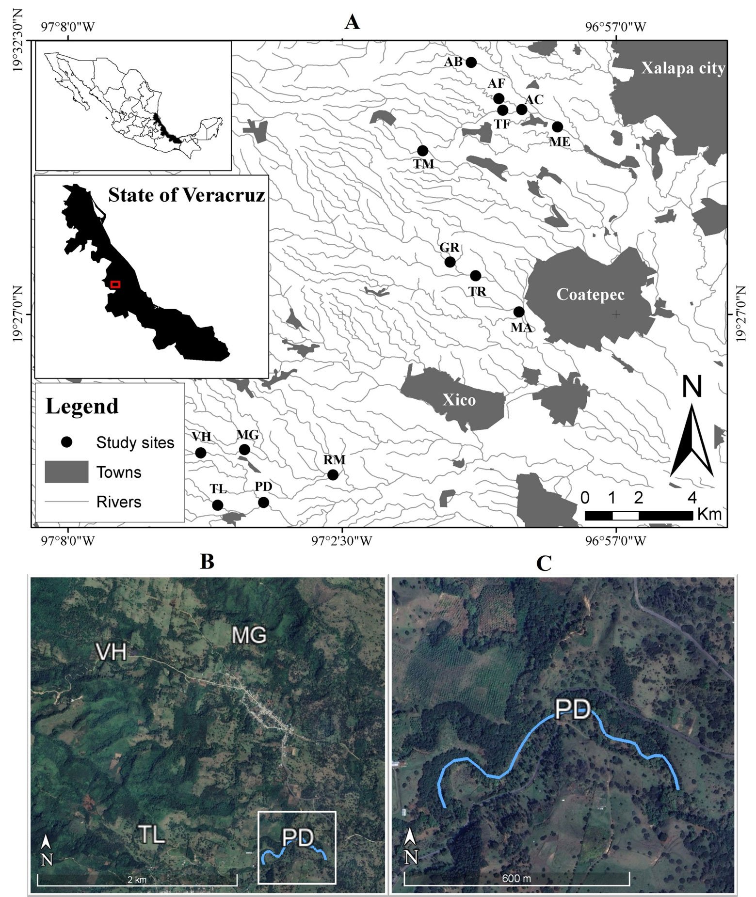
Figure 1. A, Location of the 14 segments of cloud forest riparian corridors (black circles) selected for bird sampling in central Veracruz, Mexico. The main river or streams (lines) and cities (polygons) are shown in gray. Sampling sites: Agua Bendita (AB), Agüita Fría (AF), Acuario (AC), Trucha Feliz (TF), Mariano Escobedo (ME), Truchas Martin (TM), Granada (GR), Trianon (TR), Marina (MA), Rio Matlacobatl (RM), Puente de Dios (PD), Monte Grande (MG), Tlalchy (TL) and Vista Hermosa (VH); B, image (Google Earth – Pro V 7.3.6.9345) is a close-up of 4 of the riparian corridor segments sampled (VH, MG, TL, PD); C, close-up of the PD site, with the river indicated by a blue line. Map by O. Hernández-Dávila.
Bird species were identified using the Sibley (2000) and Howell and Webb (1995) field guides. Nomenclature follows the IOC World Bird List checklist (Gill et al., 2024). Recorded birds were classified as either migratory from North America or resident species, and we also noted whether they were endemic, following Navarro-Sigüenza et al. (2007). The conservation status of each species was based on Mexican federal law NOM-059 (Semarnat 2010), and The IUCN Red List (IUCN, 2024). For trophic guild, each species was classified as: carnivore, insectivore, frugivore, granivore, nectarivore and omnivore (González-Salazar et al., 2014). Additionally, species were categorized into 3 size categories (body mass): small (< 40 g), medium (40 – 100 g) and large birds (> 100 g). Forest stratum preferences were based on Martínez-Morales (2001) and classified as: canopy species (those associated with the upper forest stratum, > 10 m above the ground); midstory species (those that preferentially use forest stratum between 5 and 10 m above the ground); midstory and canopy species (those using both midstory and canopy strata); understory species (those that frequent the forest floor up to 5 m above the ground); understory and midstory species (those using both understory and midstory strata); and all strata species (those that use all forest strata). Finally, main habitat preference was also based on Martínez-Morales (2001) and noted as: forest interior species (those which prefer forest sites away from the forest edge); forest edge species (those that preferentially use the fragment edge less than 100 m away from open areas); forest generalist species (those that are common both at the edge and the interior of forest fragments); and vegetation matrix species (those associated with the agricultural matrix or open areas). For species not reported by Martínez-Morales (2001) we did not assign categories for forest stratum preference and habitat preference. For these cases, species were classified as unknown.
The total richness recorded in riparian corridors was determined by the sum of records obtained from point records and those from mist-nets. Each bird species was characterized in relation to its migratory and conservation status, size, trophic guild, and habitat and forest stratum preferences. Due to the differences in the number of riparian corridors sampled by each sampling method (i.e., 14 for count points and 6 for mist nets) and their differences in data obtained from each method, for all the remaining analyses, only data from count points were taken into account: species accumulation curve and sample coverage were estimated to assess the sample completeness. Hill numbers were calculated to analyze the diversity of bird species in terms of effective number of species (q0), effective number of abundant species or Shannon diversity (q1) and effective number of dominant species or Simpson diversity (q2) (Hsieh et al., 2016; Jost, 2006). The rank-abundance curve of overall recorded avifauna was drawn to show graphically the structure of the bird community (Kindt & Coe, 2005). Analyses of accumulation curves, Hill numbers and range-abundance curves were performed for all riparian strips combined and separately. Finally, similarity in species composition among the 14 sampling sites was estimated using the Jaccard index distance, which varies from 0 to 1. Zero indicates that no species are shared between compared sites, and 1 indicates that species composition is identical between the sites. All analyses were run in R software using the vegan (Oksanen et al., 2020) and BiodiversityR (Kindt, 2021) packages.
Results
We recorded a total of 86 bird species in the 14 riparian corridors. These 86 species belonged to 9 orders, 27 families and 67 genera (Table 1). The richest families were Parulidae (16 species); Tyrannidae (13 spp.); Trochilidae (9 spp.) and Turdidae (6 spp.). Of the 86 bird species, there were 67 recorded at the point-counts and 48 trapped in the nets, with 29 recorded with both field methods (Table 1).
Of the 86 recorded species, 65 were resident species and 21 were migratory. Only 2 of the recorded species are endemic to Mexico: Melanotis caerulescens (Blue Mockingbird) and Cardellina rubra (Red Warbler). Four species are under special protection status by Mexican federal law (Semarnat, 2010): Accipiter striatus (Sharp-shinned Hawk), Cinclus mexicanus (American Dipper), Psarocolius montezuma (Montezuma Oropendola) and Catharus mexicanus (Black-headed Nightingale-thrush), and 1 species is threatened: Catharus frantzii (Ruddy-capped Nightingale-thrush). One species, Selasphorus rufus (Rufous Hummingbird), is regarded as Near Threatened in the IUCN list. The richest trophic guilds were insectivorous (63% of species) and frugivorous birds (15%) (Fig. 2A). Regarding forest stratum preference, 18% of the species recorded prefer the midstory to canopy strata, and 17% are midstory specialists (Fig. 2B). For habitat preference, habitat generalists were the most strongly represented accounting for 30% of richness, followed by forest-interior species with 18% (Fig. 2C). Most recorded species (66%) were relatively small with a body mass < 40 g, and only 12% of species were heavier than 100 g (Fig. 2D).
During the 28 point counts we recorded a total of 816 detections of 67 bird species using the corridors. In the mist nets placed in 6 of the corridors, we captured 273 birds belonging to 48 species. The species accumulation curve for all corridors reached a sample completeness of 97%. According to Hill numbers the bird diversity was of 67 species observed (q0), 18 common species (q1) and 8 dominant species (q2) (Fig. 3). Individually, the sample completeness for each of the 14 riparian segments varied between 79% and 93% per segment; and regarding diversity, q0 ranged from 9 to 24 bird species per segment, while q1 ranged from 5 to 13 species and q2 from 2 to 13 species (Fig. 4).
Table 1
List of the 86 bird species recorded in 14 cloud forest riparian corridors in the anthropic landscape of central Veracruz, Mexico. Shown are the number of visual detections (# detections) of each species estimated by point counts and the number of birds
captured in mist nets. Seed dispersing birds are indicated with an asterisk (*). Species are ordered by rank (only for data obtained by point counts). We also show for each species: migratory status, resident (R), North American migrant (M). Protection status: threatened (A), special protection (Pr), least concern (LC), near threatened (NT). Trophic guild: insectivore (In), frugivore (Fr), nectarivore (Ne), omnivore (Om), granivore (Gr), carnivore (Ca). Size (body mass in g): small < 40 g (1), medium-sized 40 – 100 g (2), large > 100 g (3). Habitat preference: forest interior (FI), forest edge (FE), forest generalist (FG), vegetation matrix (VM), and no information available (-). Forest stratum preference: understory (U), understory and midstory (UM), midstory (M), midstory and canopy (MC), canopy (C), and no information available (-). See below for bibliographic sources.
| Species | # detections by point counts | # captures in mist nets | Migratory status | Protection status | Trophic guild | Size category | Habitat preference | Stratum preference |
| Chlorospingus flavopectus* | 234 | 17 | R | -/LC | In-Fr | 1 | FG | MC |
| Cardellina pusilla | 102 | 15 | M | -/LC | In | 1 | FG | A |
| Psilorhinus morio* | 79 | 2 | R | -/LC | Om | 3 | FG | MC |
| Myadestes occidentalis* | 51 | 10 | R | -/LC | Fr | 2 | FG | MC |
| Empidonax difficilis | 36 | 18 | R | -/LC | In | 1 | FG | M |
| Myiozetetes similis* | 33 | 3 | R | -/LC | In-Fr | 1 | VM | C |
| Parkesia motacilla* | 20 | 14 | M | -/LC | In-Fr | 1 | FI | U |
| Psarocolius montezuma* | 20 | – | R | Pr/LC | Fr | 3 | – | – |
| Setophaga townsendi | 12 | – | M | -/LC | In | 1 | FG | MC |
| Sayornis nigricans | 11 | 2 | R | -/LC | In | 1 | – | – |
| Tityra semifasciata* | 9 | – | R | -/LC | In-Fr | 2 | – | – |
| Turdus assimilis* | 9 | 6 | R | -/LC | Fr | 2 | FE | M |
| Turdus grayi* | 9 | 6 | R | -/LC | Fr | 2 | FE | M |
| Cinclus mexicanus | 8 | – | R | Pr/LC | Ca | 2 | – | – |
| Leiothlypis ruficapilla | 8 | 1 | M | -/LC | In | 1 | FI | MC |
| Mitrephanes phaeocercus | 8 | – | R | -/LC | In | 1 | FG | M |
| Quiscalus mexicanus* | 8 | 1 | R | -/LC | Om | 3 | – | A |
| Vireo solitarius* | 8 | 3 | M | -/LC | In-Fr | 1 | FG | M |
| Henicorhina leucophrys* | 7 | 4 | R | -/LC | In-Fr | 1 | FG | U |
| Melanerpes aurifrons* | 6 | – | R | -/LC | In-Fr | 2 | – | – |
| Thraupis abbas* | 6 | 1 | R | -/LC | Fr | 2 | FE | C |
| Contopus pertinax | 5 | 1 | R | -/LC | In | 1 | FG | C |
| Cyanolyca cucullata* | 5 | – | R | -/LC | Om | 3 | FI | MC |
| Euphonia hirundinacea* | 5 | 9 | R | -/LC | Fr | 1 | – | – |
| Lepidocolaptes affinis | 5 | 3 | R | -/LC | In | 1 | FG | M |
| Mniotilta varia | 5 | 1 | M | -/LC | In | 1 | FI | MC |
| Myioborus miniatus | 5 | 1 | R | -/LC | In | 1 | FI | M |
| Chloroceryle americana | 4 | – | R | -/LC | Ca | 2 | FE | MC |
| Empidonax hammondii | 4 | – | M | -/LC | In | 1 | – | – |
| Melanerpes formicivorus* | 4 | – | R | -/LC | In-Fr | 2 | FE | MC |
| Piranga leucoptera* | 4 | – | R | -/LC | In-Fr | 1 | – | – |
| Table 1. Continued | ||||||||
| Species | # detections by point counts | # captures in mist nets | Migratory status | Protection status | Trophic guild | Size category | Habitat preference | Stratum preference |
| Catharus frantzii* | 3 | 4 | R | A/LC | Fr | 1 | FI | UM |
| Momotus coeruliceps* | 3 | 2 | R | -/LC | In-Fr | 3 | FG | M |
| Myiarchus tuberculifer* | 3 | 1 | R | -/LC | In-Fr | 1 | FG | M |
| Polioptila caerulea | 3 | – | M | -/LC | In | 1 | FG | MC |
| Ptiliogonys cinereus* | 3 | – | R | -/LC | In-Fr | 1 | FG | C |
| Rupornis magnirostris | 3 | 1 | R | -/LC | Ca | 3 | – | – |
| Vireo cassini* | 3 | – | M | -/LC | In-Fr | 1 | – | – |
| Amazona albifrons | 2 | – | R | -/LC | Gr | 3 | – | – |
| Basileuterus belli* | 2 | 11 | R | -/LC | In-Fr | 1 | FI | UM |
| Basileuterus rufifrons | 2 | – | R | -/LC | In | 1 | FG | UM |
| Chlorophonia elegantissima * | 2 | – | R | -/LC | Fr | 1 | FI | MC |
| Dendrocincla homochroa | 2 | 1 | R | -/LC | In | 2 | – | – |
| Leptotila verreauxi | 2 | – | R | -/LC | Gr | 3 | FG | U |
| Pyrocephalus rubinus | 2 | – | R | -/LC | In | 1 | – | – |
| Saltator atriceps | 2 | 2 | R | -/LC | Fr | 2 | – | – |
| Setophaga tigrina | 2 | – | M | -/LC | In | 1 | – | – |
| Setophaga virens | 2 | – | M | -/LC | In | 1 | FI | MC |
| Sporophila morelleti | 2 | 1 | R | -/LC | Gr | 1 | – | – |
| Campylorhynchus zonatus | 1 | – | R | -/LC | In | 2 | – | – |
| Cardellina rubra | 1 | – | R | -/LC | In | 1 | – | – |
| Catharus mexicanus* | 1 | 12 | R | Pr/LC | Fr | 1 | FG | U |
| Corthylio calendula | 1 | – | M | -/LC | In | 1 | FG | U |
| Dives dives* | 1 | 2 | R | -/LC | In-Fr | 2 | VM | A |
| Dumetella carolinensis* | 1 | 2 | M | -/LC | In-Fr | 2 | VM | M |
| Empidonax minimus | 1 | – | M | -/LC | In | 1 | – | – |
| Icterus bullockii* | 1 | – | R | -/LC | In-Fr | 1 | FE | M |
| Megarynchus pitangua* | 1 | – | R | -/LC | In-Fr | 2 | – | – |
| Ortalis vetula* | 1 | – | R | -/LC | Fr | 3 | FE | M |
| Pachyramphus aglaiae | 1 | – | R | -/LC | In | 1 | FI | MC |
| Piaya cayana* | 1 | – | R | -/LC | In-Fr | 3 | FG | M |
| Piranga flava* | 1 | – | R | -/LC | In-Fr | 1 | FE | MC |
| Piranga rubra* | 1 | – | M | -/LC | In-Fr | 1 | FI | MC |
| Seiurus aurocapilla | 1 | 1 | M | -/LC | In | 1 | FI | U |
| Setophaga nigrescens | 1 | – | M | -/LC | In | 1 | – | – |
| Setophaga ruticilla | 1 | – | M | -/LC | In | 1 | – | – |
| Tyrannus melancholicus | 1 | – | R | -/LC | In | 1 | VM | C |
| Accipiter striatus | – | 1 | R | Pr/LC | Ca | 3 | – | – |
| Archilochus colubris | – | 1 | M | -/LC | Ne | 1 | FI | UM |
| Table 1. Continued | ||||||||
| Species | # detections by point counts | # captures in mist nets | Migratory status | Protection status | Trophic guild | Size category | Habitat preference | Stratum preference |
| Arremon brunneinucha* | – | 14 | R | -/LC | In-Fr | 2 | FG | M |
| Basileuterus culicivorus | – | 2 | R | -/LC | In | 1 | FG | UM |
| Campylopterus hemileucurus | – | 20 | R | -/LC | Ne | 1 | – | – |
| Cardellina canadensis | – | 1 | M | -/LC | In | 1 | FI | U |
| Catharus aurantiirostris* | – | 2 | R | -/LC | Fr | 1 | FG | U |
| Chlorestes candida | – | 1 | R | -/LC | Ne | 1 | – | – |
| Eugenes fulgens | – | 2 | R | -/LC | Ne | 1 | FE | M |
| Lampornis amethystinus | – | 21 | R | -/LC | Ne | 1 | FG | U |
| Melanotis caerulescens* | – | 1 | R | -/LC | In-Fr | 2 | FE | U |
| Myiodynastes luteiventris* | – | 2 | R | -/LC | In-Fr | 2 | FI | MC |
| Pampa curvipennis | – | 12 | R | -/LC | Ne | 1 | VM | UM |
| Pitangus sulphuratus* | – | 1 | R | -/LC | In-Fr | 2 | FG | A |
| Saucerottia beryllina | – | 12 | R | -/LC | Ne | 1 | – | – |
| Saucerottia cyanocephala | – | 19 | R | -/LC | Ne | 1 | FE | UM |
| Selasphorus rufus | – | 1 | M | -/NT | Ne | 1 | – | – |
| Stelgidopteryx serripennis | – | 1 | R | -/LC | In | 1 | FG | C |
| Vireo gilvus* | – | 1 | R | -/LC | In-Fr | 1 | FI | C |
*Seed dispersing birds: based on field data from Hernández-Dávila et al. (2022) and Hernández-Ladrón De Guevara et al. (2012). Migratory status: from Howell and Webb (1995) and Sibley (2000). Size: from Martínez-Morales (2001), Sibley (2000), and birds captured in mist nets (this study). Habitat preference and stratum preference: from Martínez-Morales (2001).
The most common species recorded visually was Chlorospingus flavopectus (Common Chlorospingus) with 234 detections (Fig. 5A), followed by Cardellina pusilla (Wilson’s Warbler) with 102, Psilorhinus morio (Brown Jay) with 79 and Myadestes occidentalis (Brown-backed Solitaire) with 51 detections (see species detection data in Table 1). These 4 dominant species accounted for 45% of total detections recorded in the point counts. There were 10 species with only 2 detections (i.e., doubletons) and 18 species with only 1 (singletons), and these 28 extremely rare species accounted for less than 5% of total detections and 42% of the 67 species recorded in the point counts. In general, the pattern of dominance by the 4 species mentioned occurred in each riparian corridor sampled, concentrating most of the bird detections at each site, with several species having much fewer detections per site (Fig. 5B).
Bird species richness per site estimated in point counts varied from 9 (TM site) to 33 species (MA site), with 10 of the 14 segments sampled having fewer than 20 species each. Similarity between sites was low (Jaccard index, J < 0.4) for most of the paired comparisons (Table 2), with the highest level of similarity between the TL and AB sites (0.53) and the lowest between MA and AF (0.10).
Discussion
In general, and pooling all sampled riparian corridors, the sample completeness was high (97%), recording a total richness of 86 bird species in the 14 segments sampled in the fragmented cloud forest landscape of central Veracruz, Mexico. This richness is comparable to that reported in similar studies carried out in relatively large (> 3 ha) remnant fragments of cloud forest in the same region, where up to 75-100 bird species have been detected (Rueda-Hernández et al., 2015; Serna-Lagunes et al., 2023). These 14 riparian corridors harbor 24% of the bird richness reported for cloud forest throughout the entire state of Veracruz (Navarro-Sigüenza et al., 2014). The richness recorded in our study represents between 25 and 43% of the avifauna reported in other regions of Mexico with cloud forest, where 196 to 335 bird species have been found (Martínez-Morales, 2007; Navarro-Sigüenza et al., 2014). The richness detected suggests that riparian corridors are important elements in deforested landscapes of cloud forest for numerous birds. Other studies in different sites have shown that these elements of the landscape can serve as refuges, foraging areas and even as reproductive (nesting) sites (Hawes et al., 2008; de Zwaan et al., 2022), as well as making it possible for birds to move across large open areas in agricultural landscapes (Gillies & St. Clair, 2010; Pliscoff et al., 2020). Both resident species and migratory birds, visit and use forested riparian corridors during their autumn-winter stay in the tropics (Skagen et al., 1998; Villaseñor-Gómez, 2008). As shown in our results: 24% of the recorded species were North American migratory species. The migratory bird Cardellina pusilla, abundant in cloud forest as well as in shaded coffee plantations in Veracruz (Navarro-Sigüenza et al., 2014), was the second most common species in our study. By far, the most dominant species in our study was Chlorospingus flavopectus, a resident bird regarded as a forest generalist that is common to old-growth forest, forest edge habitats and patches of secondary forest (Cruz-Angón et al., 2008; Martínez-Morales, 2007; Renner et al., 2006). Myadestes occidentalis was the fourth most dominant species in riparian corridors, which is considered a typical cloud forest species (Caballero-Cruz et al., 2020). This pattern of dominance is similar to that recorded by Martínez-Morales (2001) who reported C. flavopectus, M. occidentalis, Henicorhina leucophrys, Catharus mexicanus, and Trogon mexicanus as the most dominant species in conserved fragments of cloud forest. Except for T. mexicanus, the mentioned species were recorded in this study. Another very common bird in our study was Psilorhinus morio, a habitat generalist associated with disturbed areas, and common in small forest fragments of cloud forest (Serna-Lagunes et al., 2023), in rainforest riparian corridors that cross pastures (Graham et al., 2002), as well as in open agricultural areas with scant arboreal cover (Cerezo et al., 2009). It is important to mention that P. morio is a large species (> 100 gr), only 12% of the species recorded belong to this size category, while 65% are small species (< 40 gr). The conversion of forest for agricultural purposes mainly affects the presence of large bird species due to the reduction in food availability as well as fewer nesting and roosting sites (Gomes et al., 2008; Martínez-Morales, 2001). Thus, large bird species are the most strongly affected by the reduction of forest cover, while small birds are more vagile and tolerant to deforestation, explaining the predominance of species smaller than 40 g in the riparian corridors studied.
Table 2
Similarity distance in bird species composition (Jaccard index) among the 14 riparian corridors sampled (upper-right side of Table) with point counts (see Materials and methods), showing the number of species shared between riparian corridors (lower-left side), and the total number of species in each corridor (diagonal black cells). Gray-shaded cells highlight the highest and lowest values of similarity distance. The names of riparian corridors sampled are abbreviated as in Figure 1.
| AC | AB | AF | TR | GR | MA | ME | MG | PD | RM | TL | TF | TM | VH | |
| AC | 21 | 0.36 | 0.39 | 0.39 | 0.37 | 0.26 | 0.31 | 0.37 | 0.43 | 0.29 | 0.26 | 0.34 | 0.30 | 0.27 |
| AB | 9 | 13 | 0.33 | 0.35 | 0.43 | 0.24 | 0.30 | 0.38 | 0.39 | 0.32 | 0.53 | 0.35 | 0.38 | 0.32 |
| AF | 9 | 6 | 11 | 0.21 | 0.24 | 0.10 | 0.14 | 0.29 | 0.36 | 0.17 | 0.33 | 0.26 | 0.43 | 0.28 |
| TR | 11 | 8 | 5 | 18 | 0.52 | 0.24 | 0.29 | 0.21 | 0.32 | 0.27 | 0.19 | 0.29 | 0.23 | 0.25 |
| GR | 11 | 10 | 6 | 13 | 20 | 0.33 | 0.32 | 0.24 | 0.39 | 0.33 | 0.27 | 0.36 | 0.32 | 0.33 |
| MA | 11 | 9 | 4 | 10 | 13 | 33 | 0.31 | 0.17 | 0.27 | 0.43 | 0.21 | 0.28 | 0.17 | 0.25 |
| ME | 9 | 6 | 3 | 7 | 8 | 11 | 13 | 0.21 | 0.33 | 0.37 | 0.18 | 0.35 | 0.29 | 0.25 |
| MG | 10 | 8 | 6 | 6 | 7 | 7 | 5 | 16 | 0.35 | 0.25 | 0.32 | 0.42 | 0.32 | 0.27 |
| PD | 12 | 9 | 8 | 9 | 11 | 11 | 8 | 9 | 19 | 0.30 | 0.33 | 0.48 | 0.33 | 0.35 |
| RM | 10 | 9 | 5 | 9 | 11 | 17 | 10 | 8 | 8 | 24 | 0.32 | 0.40 | 0.22 | 0.24 |
| TL | 7 | 9 | 6 | 5 | 7 | 8 | 4 | 7 | 7 | 9 | 13 | 0.29 | 0.29 | 0.25 |
| TF | 10 | 8 | 6 | 8 | 10 | 11 | 8 | 10 | 12 | 12 | 7 | 18 | 0.35 | 0.43 |
| TM | 7 | 6 | 6 | 5 | 7 | 6 | 5 | 6 | 8 | 6 | 5 | 7 | 9 | 0.40 |
| VH | 7 | 6 | 5 | 6 | 8 | 9 | 5 | 6 | 10 | 7 | 5 | 9 | 6 | 12 |
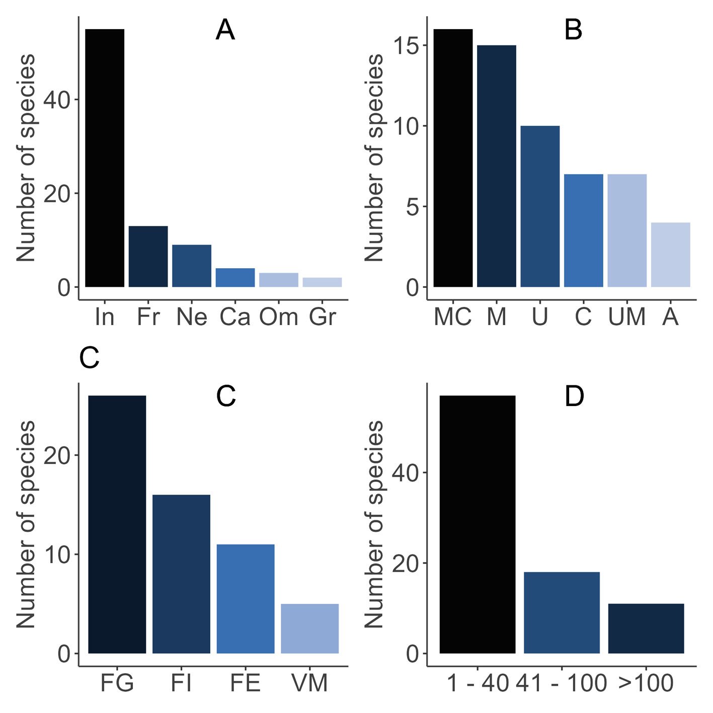
Figure 2. Characterization of the avifauna recorded in 14 segments of cloud forest riparian corridors sampled in central Veracruz, Mexico. A, Trophic guild: insectivore (In), frugivore (Fr), nectarivore (Ne), carnivore (Ca), omnivore (Om), and granivore (Gr); B, forest stratum preference: canopy (C), midstory and canopy (MC), midstory (M), understory and midstory (UM), understory (U), and all strata (A); C, habitat preference: forest generalist (FG), forest interior (FI), forest edge (FE), and vegetation matrix (VM); D, size (body mass): small (1 – 40 g), medium (40 – 100 g) and large (100 – 500 g).
Insectivorous birds were the richest and most abundant trophic guild in the riparian corridors sampled and are also the most common guild in intact cloud forest (Martínez-Morales, 2007). Frugivorous birds were the second richest guild and were relatively abundant in our riparian corridors. These species, together with omnivorous species, are particularly important in forest regeneration due to their role as seed dispersers of forest plants. Some of the most important frugivores that are efficient dispersers of cloud forest trees, shrubs and other zoochorous plants include M. occidentalis, C. flavopectus, P. morio, and several species of the genera Turdus, Catharus, and Euphonia (Hernández-Dávila et al., 2022; Hernández-Ladrón De Guevara et al., 2012), all of which were recorded in our study. Seed dispersal by birds is crucial for cloud forest restoration since most plant species native to this forest depend on vertebrate frugivores for dispersal (Jordano et al., 2011). Forest frugivores usually avoid open areas that are devoid of perching sites, and this is one of the strongest limitations to forest restoration due to the limited or absent immigration of woody plant seeds into agricultural areas (Holl et al., 2000). However, it has been recorded that the density of linear forest or wooded patches such as riparian strips and live fences can increase bird diversity in agricultural landscapes (Wilson et al., 2017). In this sense cloud forest riparian corridors could contribute to species movement across the landscape. Thus, forested riparian corridors within the agricultural matrix facilitate that frugivorous birds will visit these disturbed sites and disperse seeds across and into the site. Another group of birds that is crucial for plant reproduction are the nectarivorous species, with several species of hummingbirds being particularly important. Of the 26 hummingbird species reported for Mexican cloud forest (Navarro-Sigüenza et al., 2014), 9 were recorded in the riparian corridors that we studied. The presence of birds that are seed or pollen vectors in riparian corridors contributes greatly to connectivity in anthropic landscapes and are essential to biodiversity conservation and forest regeneration and restoration in these landscapes.
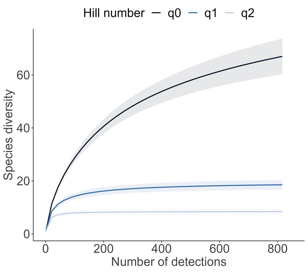
Figure 3. Species accumulation curve and Hill numbers of the bird community recorded in 14 cloud forest riparian corridors. Shaded area delimits 95% confidence intervals.
As expected by the high degree of anthropic disturbance in the landscape we studied, the richest groups of birds in the cloud forest riparian corridors were forest generalist species and those associated with the vegetation of the agricultural matrix (sensu Martínez-Morales, 2001), which together represented 53% of the avifauna we recorded. The presence and wide distribution of different arboreal elements within the current anthropic landscape could explain the presence of forest interior bird species in riparian corridors. Changes in the structure and floristic composition of the original vegetation of a given site, resulting from human activities also lead to changes in the community attributes of the avifauna (Martínez-Morales, 2005). Among the most salient changes in the forested riparian corridors that cross agricultural areas is the high abundance of plants that are common in large canopy gaps or associated with disturbed sites, including several species of the families Piperaceae, Melastomataceae, and Rubiaceae, which were common in our study (Hernández-Dávila et al., 2020). These vegetation changes are more favorable to habitat generalists than to bird species associated with the interior of large forest fragments, explaining the lower proportion of species whose preferred habitat is the forest interior in our results. Studies in different regions report an increase in the richness and abundance of habitat generalist birds in forest edge habitats, where forest interior birds decrease (de Zwaan et al., 2022; Watson et al., 2004; Wilson et al., 2017).
For cloud forest, Martínez-Morales (2005) found that fragment size positively affects the richness and abundance of both generalist and forest-interior birds. In addition, for riparian corridors of cloud forest, Hernández-Davila et al. (2021) found that the richness and abundance of generalist and specialist birds showed a differential response to the amount of forest and urban cover in the vicinity of riparian strips. The percentage of urban cover near the riparian strip negatively affected the abundance of forest interior species and positively affected generalist species, whereas surprisingly the amount of forest area nearby the strip does not seem to influence the richness and abundance of birds using the riparian strip. These results could explain the differences between the number of generalist and interior species found in our study, as well as the differences of the Hill diversity values among the sampled corridors. Although this study did not analyze explicitly aspects of landscape configuration, it is relevant to mention that, although the riparian corridors are narrow remnants of just a few meters wide (< 10 m), both generalist and forest interior species were recorded in them. This suggests that these remnants may harbor a wealth of bird species regardless of their habitat preference. In fact, 2 of the bird species recorded are endemic to Mexico, another 4 are protected by law and 1 is threatened. This highlights the importance of riparian corridors as reservoirs of birds within anthropic landscapes, particularly species native to the cloud forest including resident and migratory birds. It is important to note that 3 of the species recorded in riparian corridors; Quiscalus mexicanus, Rupornis magnirostris, and Pyrocephalus rubinus could be regarded as urban birds (Maya-Elizarrarás, 2011; Ruelas & Aguilar, 2010).
As far as we know, this study is the first to describe and characterize the avifauna present in riparian corridors of the threatened cloud forest, however, it is important to take into account that, despite the fact that our point counts had a sufficient separation and elapsed time between observations to warrant independent detections and no overflying individuals or auditory recordings were included, we might have overestimated species abundances, in particular because birds move frequently along the forest strips (personal observation, OHD). Also, because mist nets capture understory species more frequently, species richness of mid- to high- strata birds are usually underestimated with nets. This study focused on riparian corridors and did not include other types of natural remnants or conserved forest fragments present in the region and part of the current mosaic of the anthropic fragmented landscape. Therefore, more studies are needed to determine the importance of riparian corridors for conserving bird diversity in comparison with other natural remnants of cloud forest.
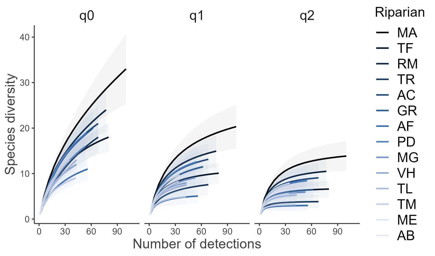
Figure 4. Species accumulation curve and Hill numbers (q0, q1, and q2) of birds recorded in each riparian corridor. Sites are ordered according to richness; dark blue curves correspond to the riparian corridors with the highest richness (e.g., MA), while light blue curves correspond to the sites with the lowest richness (e.g., AB). Shaded area delimits 95% confidence intervals. Abbreviations of riparian corridors can be found in Figure 1.
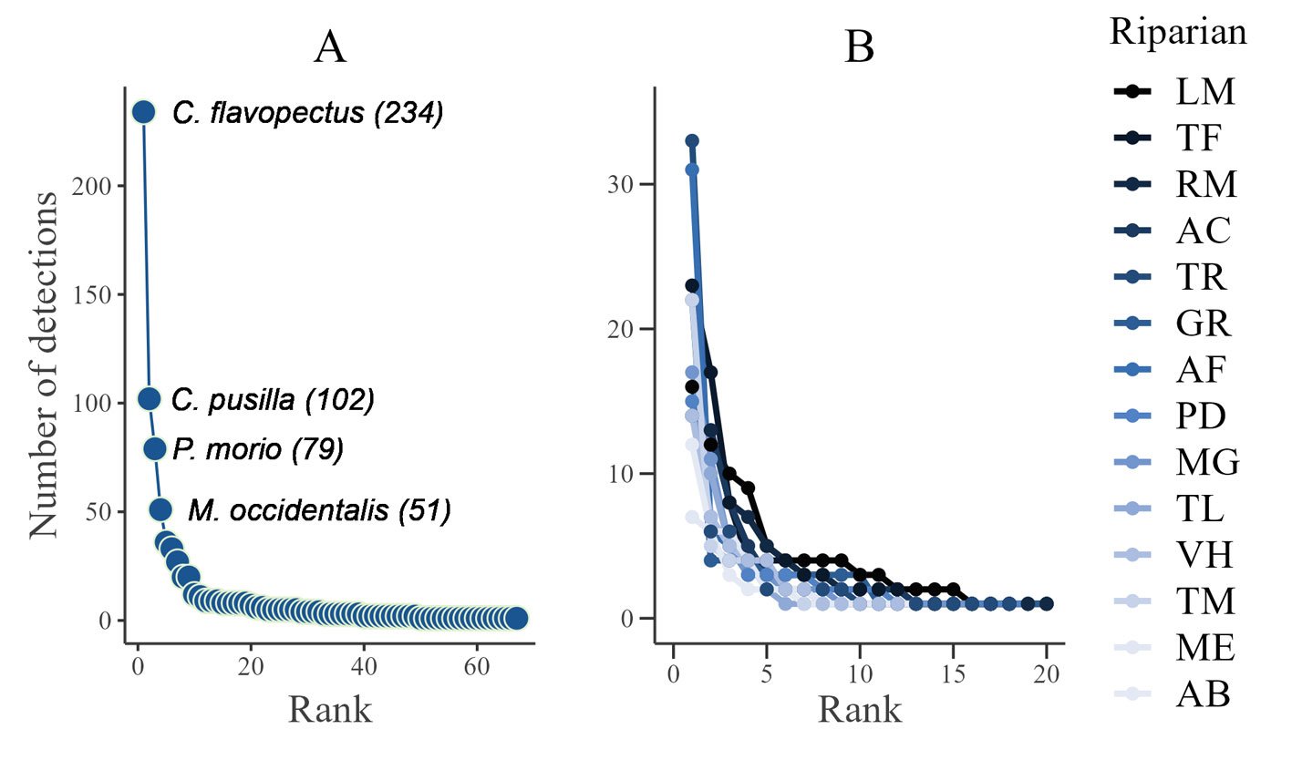
Figure 5. A, Rank-abundance curve for the avifauna recorded in 14 segments of cloud forest riparian corridors in central Veracruz, Mexico. The 4 most common species were: C. flavopectus, C. pusilla, P. morio, and M. occidentalis, the number of total detections is given in parenthesis; B, Rank-abundance curve in each riparian corridor. Sites are ordered according to number of detections; dark blue curves correspond to the riparian corridors with the highest number of detections (e.g., LM), while light blue curves correspond to the sites with the lowest number of detections (e.g., AB). Abbreviations of riparian corridors can be found in Figure 1.
In conclusion, our results show that the cloud forest riparian corridors that cross open agricultural areas harbor a diverse assemblage of bird species, which includes not only those tolerant of or associated with disturbance, but also species that are typical of intact patches of old-growth cloud forest. These would be absent in areas that are completely devoid of trees. Additionally, several of the birds recorded in our study are effective seed dispersers of cloud forest plants. For current deforested landscapes, this strongly suggests that cloud forest riparian corridors could be key elements in forest restoration efforts and for the conservation of bird biodiversity in agricultural landscapes. Landscape management plans designed to encourage the permanence and sustainable management of these forested corridors within the agricultural matrix will not only help in the conservation of the avifauna, but also in the restoration of degraded landscapes, thanks to the ecosystem services provided by birds, including the pollination and seed dispersal of plants native to the cloud forest.
Acknowledgement
We are grateful to María de los Ángeles García and Diana Vázquez for their valuable help in the field. The Instituto de Ecología, A.C. and Idea Wild provided the space and equipment that made this study possible. Bianca Delfosse translated the text from the original in Spanish and edited subsequent versions of the manuscript. We also thank two anonymous reviewers for their suggestions to improve the manuscript. This work was supported by The Rufford Foundation (grant number 20471-1 to OHD) and the Consejo Nacional de Ciencia y Tecnología (grant numbers CONACYT-CB-2016-01 to VJS, and graduate scholarship CONACYT-285962 to OHD).
References
Aldrich, M., Bubb, P., Hostettler, S., & van de Wiel, H. (2000). Tropical montane cloud forests: time for action. WWF International/IUCN The World Conservation Union.
Arizmendi, M. D. C., Dávila, P., Estrada, A., Figueroa, E., Márquez-Valdelamar, L., Lira, R. et al. (2008). Riparian Mesquite bushes are important for bird conservation in tropical arid Mexico. Journal of Arid Environments, 72, 1146–1163. https://doi.org/https://doi.org/10.1016/j.jaridenv.2007.12.017
Bonilla-Moheno, M., & Aide, T. M. (2020). Beyond deforestation: Land cover transitions in Mexico. Agricultural Systems, 178, 102734. https://doi.org/https://doi.org/10.1016/j.agsy.2019.102734
Bruijnzeel, L. A., Scatena, F. N., & Hamilton, L. S. (2011). Tropical montane cloud forests. Science for conservation and management (International Hydrology Series). Cambridge University Press.
Caballero-Cruz, P., Vargas-Noguez, G., & Ortiz-Pulido, R. (2020). Especies de aves en riesgo en el bosque mesófilo de montaña en cinco AICA de la sierra Madre Oriental, México. Huitzil, Revista Mexicana de Ornitología, 21, e-490. https://doi.org/https://doi.org/10.28947/hrmo.2020.21.1.472
Cerezo, A., Robbins, C. S., & Dowell, B. (2009). Uso de hábitats modificados por aves dependientes de bosque tropical en la región caribeña de Guatemala. Revista de Biología Tropical, 57, 401–419. https://doi.org/https://doi.org/10.15517/rbt.v57i1-2.11355
Cole, L. J., Stockan, J., & Helliwell, R. (2020). Managing riparian buffer strips to optimise ecosystem services: A review. Agriculture, Ecosystems and Environment, 296, 106891. https://doi.org/https://doi.org/10.1016/j.agee.2020.106891
Cruz-Angón, A., Scott, S. T., & Greenberg, R. (2008). An experimental study of habitat selection by birds in a coffee plantation. Ecology, 89, 921–927. https://doi.org/https://doi.org/10.1890/07-0164.1
de Zwaan, D. R., Alavi, N., Mitchell, G. W., Lapen, D. R., Duffe, J., & Wilson, S. (2022). Balancing conservation priorities for grassland and forest specialist bird communities in agriculturally dominated landscapes. Biological Conser-
vation, 265, 109402. https://doi.org/10.1016/j.biocon.2021.109402
Domínguez-López, M. E., & Ortega-Álvarez, R. (2014). The importance of riparian habitats for avian communities in a highly human-modified Neotropical landscape. Revista Mexicana de Biodiversidad, 85, 1217–1227. https://doi.org/10.7550/rmb.43849
Gill, F., Donsker, D., & Rasmussen, P. (2024). IOC World Bird List (v14.1). https://www.worldbirdnames.org/new/
Gillies, C. S., & St. Clair, C. C. (2010). Functional responses in habitat selection by tropical birds moving through fragmented forest. Journal of Applied Ecology, 47, 182–190. https://doi.org/10.1111/j.1365-2664.2009.01756.x
Gomes, G. L. L., Oostra, V., Nijman, V., Cleef, A. M., & Kappelle, M. (2008). Tolerance of frugivorous birds to habitat disturbance in a tropical cloud forest. Biological Conservation, 141, 860–871. https://doi.org/10.1016/j.biocon.2008.01.007
González-Salazar, C., Martínez-Meyer, E., & López-Santiago, G. (2014). A hierarchical classification of trophic guilds for North American birds and mammals. Revista Mexicana de Biodiversidad, 85, 931–941. https://doi.org/10.7550/rmb.38023
Graham, C., Martínez-Leyva, J. E., & Cruz-Paredes, L. (2002). Use of fruiting trees by birds in continuous forest and riparian forest remnants in Los Tuxtlas, Veracruz, Mexico. Biotropica, 34, 589–597. https://doi.org/10.1111/j.1744-7429.2002.tb00578.x
Gregory, R. D., Gibbons, D. W., & Donald, P. F. (2004). Bird census and survey techniques. In W. J. Sutherland, I. Newton, and R. Green (Eds.), Bird ecology and conservation: a handbook of techniques (pp. 17–56). Oxford: Oxford University Press.
Griscom, H. P., Kalko, E. K., & Ashton, M. S. (2007). Frugivory by small vertebrates within a deforested, dry tropical region of Central America. Biotropica, 39, 278–282. https://doi.org/10.1111/j.1744-7429.2006.00242.x
Gual-Díaz, M., & Rendón-Correa, A. (2014). Bosques mesófilos de montaña de México: diversidad, ecología y manejo. México D.F.: Comisión Nacional para el Conocimiento y Uso de la Biodiversidad.
Hawes, J., Barlow, J., Gardner, T. A., & Peres, C. A. (2008). The value of forest strips for understorey birds in an Amazonian plantation landscape. Biological Conservation, 141, 2262–2278. https://doi.org/10.1016/j.biocon.2008.06.017
Hernández-Baños, B. E., Peterson, A. T., Navarro-Sigüenza, A. G., & Escalante-Pliego, P. B. (1995). Bird faunas of the humid montane forests of Mesoamerica: biogeographic patterns and priorities for conservation. Bird Conservation International, 5, 251–277. https://doi.org/10.1017/S0959270900001039
Hernández-Dávila, O. A., Laborde, J., Sosa, V. J., & Díaz-Castelazo, C. (2022). Interaction network between frugivorous birds and zoochorous plants in cloud forest riparian strips immersed in anthropic landscapes. Avian Research, 13, 100046. https://doi.org/10.1016/j.avrs.2022.100046
Hernández-Dávila, O. A., Laborde, J., Sosa, V. J., Gallardo-Hernández, C., & Díaz-Castelazo, C. (2020). Forested riparian belts as reservoirs of plant species in fragmented landscapes of tropical mountain cloud forest. Botanical Sciences, 98, 288–304. https://doi.org/https://doi.org/10.17129/botsci.2497
Hernández-Dávila, O. A., Sosa, V. J., & Laborde, J. (2021). Effects of landscape context and vegetation attributes on understorey bird communities of cloud forest riparian belts. Ecological Engineering, 167, 106269. https://doi.org/10.1016/j.ecoleng.2021.106269
Hernández-Ladrón De Guevara, I., Rojas-Soto, O. R., López-Barrera, F., Puebla-Olivares, F., & Díaz-Castelazo, C. (2012). Dispersión de semillas por aves en un paisaje de bosque mesófilo en el centro de Veracruz, México: Su papel en la restauración pasiva. Revista Chilena de Historia Natural, 85, 89–100. https://doi.org/10.4067/S0716-078X2012000100007
Holl, K. D., Loik, M. E., Lin, E. H. V., & Samuels, I. A. (2000). Tropical montane forest restoration in Costa Rica: overcoming barriers to dispersal and establishment. Restoration Ecology, 8, 339–349. https://doi.org/https://doi.org/10.1046/j.1526-100x.2000.80049.x
Howell, N. G., & Webb, S. (1995). A guide to the birds of Mexico and Northern Central America. Oxford: Oxford University Press.
Hsieh, T. C., Ma, K. H., & Chao, A. (2016). iNEXT: an R package for rarefaction and extrapolation of species diversity (Hill numbers). Methods in Ecology and Evolution, 7, 1451–1456. https://doi.org/10.1111/2041-210X.12613
IUCN (08 de junio de 2024). The IUCN Red List of Threatened Species. Version 2024-1. https://www.iucnredlist.org
Jordano, P., Pierre-Michel, F., Lambert, J. E., Böhning-Gaese, K., Traveset, A., & Wright, S. J. (2011). Frugivores and seed dispersal: mechanisms and consequences for biodiversity of a key ecological interaction. Biology Letters, 7, 321–323. https://doi.org/https://doi.org/10.1098/rsbl.2010.0986
Jost, L. (2006). Entropy and diversity. Oikos, 113, 363–375. https://doi.org/https://doi.org/10.1111/j.2006.0030-1299.14714.x
Karger, D. N., Kessler, M., Lehnert, M., & Jetz, W. (2021). Limited protection and ongoing loss of tropical cloud forest biodiversity and ecosystems worldwide. Nature Ecology and Evolution, 5, 854–862. https://doi.org/10.1038/s41559-021-01450-y
Kindt, R. (2021). BiodiversityR. Package for Community Ecology and Suitability Analysis (2.16-1). http://www.worldagroforestry.org/output/tree-diversity-analysis
Kindt, R., & Coe, R. (2005). Tree diversity analysis. A manual and software for common statistical methods for ecological and biodivserity studies. Nairobi: World Agroforestry Centre (ICRAF).
Kontsiotis, V., Zaimes, G. N., Tsiftsis, S., Kiourtziadis, P., & Bakaloudis, D. (2019). Assessing the influence of riparian vegetation structure on bird communities in agricultural Mediterranean landscapes. Agroforestry Systems, 93, 675–687. https://doi.org/10.1007/s10457-017-0162-x
Latta, S. C., De La Cueva, H., & Harper, A. B. (2012). Abundance and site fidelity of migratory birds wintering in riparian habitat of Baja California. Western Birds, 43, 90–101.
Lees, A. C., & Peres, C. A. (2008). Conservation value of remnant riparian forest corridors of varying quality for amazonian birds and mammals. Conservation Biology, 22, 439–449. https://doi.org/10.1111/j.1523-1739.2007.00870.x
Martínez-Morales, M. A. (2001). Forest fragmentation effects on bird communities of tropical montane cloud forests in eastern Mexico (Ph.D. Thesis). Cambridge UK: University of Cambridge.
Martínez-Morales, M. A. (2005). Landscape patterns influencing bird assemblages in a fragmented Neotropical cloud forest. Biological Conservation, 121, 117–126. https://doi.org/10.1016/j.biocon.2004.04.015
Martínez-Morales, M. A. (2007). Avifauna del bosque mesófilo de montaña del noreste de Hidalgo, México. Revista Mexicana de Biodiversidad, 78, 149–162. https://doi.org/https://revista.ib.unam.mx/index.php/bio/article/view/395
Maya-Elizarrarás, E. (2011). Aves explotadoras de áreas verdes urbanas: un ejemplo de la zona metropolitana de Guadalajara, Jalisco. El Canto Del Cenzontle, 2, 104–109.
Muñoz-Villers, L. E., & López-Blanco, J. (2008). Land use/cover changes using Landsat TM/ETM images in a tropical and biodiverse mountainous area of central-eastern Mexico. International Journal of Remote Sensing, 29, 71–93. https://doi.org/10.1080/01431160701280967
Navarro-Sigüenza, A. G., Lira-Noriega, A., Peterson, A. T., Oliveras de Ita, A., & Gordillo-Martínez, A. (2007). Diversidad, endemismo y conservación de las aves. In I. Luna, J. J. Morrone, & D. Espinosa (Eds.), Biodiversidad de la Faja Volcánica Transmexicana (pp. 461–483). México D.F.: Universidad Nacional Autónoma de México.
Navarro-Sigüenza, A. G., Gómez de Silva, H., Gual-Díaz, M., Sánchez-Gonzales, L. A., & Pérez-Villafaña, M. (2014). La importancia de las aves del bosque mesófilo de montaña de México In M. Gual-Díaz, & A. Rendón-Correa (Eds.), Bosques mesófilos de montaña de México: diversidad, ecología y manejo (pp. 279–299). Conabio.
Oksanen, J., Guillaume, B. F., Kindt, R., Legendre, P., McGlinn, D., Minchin, P. R. et al. (2020). Community Ecology Package (2.5-7). http://mirror.bjtu.edu.cn/cran/web/packages/vegan/vegan.pdf
Pliscoff, P., Simonetti, J. A., Grez, A. A., Vergara, P. M., & Barahona-Segovia, R. M. (2020). Defining corridors for movement of multiple species in a forest-plantation landscape. Global Ecology and Conservation, 23, e011108. https://doi.org/10.1016/j.gecco.2020.e01108
Renner, S. C., Walterrt, M., & Mühllenberg, M. (2006). Comparison of bird communities in primary vs. young secondary tropical montane cloud forest in Guatemala. Biodiversity and Conservation, 15, 1545–1575. https://doi.org/10.1007/s10531-005-2930-6
Rodríguez-Mendoza, C., & Pineda, E. (2010). Importance of riparian remnants for frog species diversity in a highly fragmented rainforest. Conservation Biology, 6, 781–784. https://doi.org/10.1098/rsbl.2010.0334
Rueda-Hernández, R., MacGregor-Fors, I., & Renton, K. (2015). Shifts in resident bird communities associated with cloud forset patch size in Central Veracruz, Mexico. Avian Conservation and Ecology, 10. https://doi.org/http://dx.doi.org/10.5751/ACE-00751-100202
Ruelas, I. E., & Aguilar, R. S. H. (2010). La avifauna urbana del parque ecológico Macuiltépetl en Xalapa. Ornitología Neotropical, 21, 87–103.
Semarnat (Secretaría del Medio Ambiente y Recursos Naturales). (2010). Norma Oficial Mexicana NOM-059-SEMARNAT-2010, Protección ambiental – Especies nativas de México de flora y fauna silvestres – Categorías de riesgo y especificaciones para su inclusión, exclusión o cambio – Lista de especies en riesgo. Diario Oficial de la Federación. 30 de diciembre de 2010, Segunda Sección, México.
Serna-Lagunes, R., Torres-Cantú, G. B., & García-Martínez, M. Á. (2023). Avifauna en fragmentos de bosque mesófilo de montaña y vegetación secundaria en el municipio de Huatusco, Veracruz. CienciaUAT, 1, 06–24. https://doi.org/https://doi.org/10.29059/cienciauat.v18i1.1669
Sibley, D. A. (2000). The Sibley guide to birds. New York: Alfred A. Knopf.
Skagen, S. K., Melcher, C. P., Howe, W. H., & Knopf, F. L. (1998). Comparative use of riparian corridors and oases by migrating birds in southeast Arizona. Conservation Biology, 12, 896–909. https://doi.org/https://doi.org/10.1111/j.1523-1739.1998.96384.x
Toledo-Aceves, T., García-Franco, J., Williams-Linera, G., Mac-Millan, K., & Gallardo-Hernández, C. (2014). Significance of remnant cloud forest fragments as reservoirs of tree and epiphytic bromeliad diversity. Tropical Conservation Science, 7, 230–243. https://doi.org/10.1177/194008291400700205
Toledo-Aceves, T., Meave, J., González-Espinosa, M., & Ramírez-Marcial, N. (2011). Tropical montane cloud forests: Current threats and opportunities for their conservation and sustainable management in Mexico. Journal of Environmental Management, 92, 974–981. https://doi.org/10.1016/j.jenvman.2010.11.007
Villaseñor-Gómez, J. F. (2008). Habitat use of wintering bird communities in Sonora Mexico: the importance of riparian habitats. Studies in Avian Biology, 37, 53–68.
Watson, J. E. M., Whittaker, R. J., & Dawson, T. P. (2004). Habitat structure and proximity to forest edge affect the abundance and distribution of forest-dependent birds in tropical coastal forests of southeastern Madagascar. Biological Conservation, 120, 311–327. https://doi.org/10.1016/j.biocon.2004.03.004
Williams-Linera, G., Manson, R. H., & Isunza, V. E. (2002). La fragmentación del bosque mesófilo de montaña y patrones de uso del suelo en la región oeste de Xalapa, Veracruz, México. Madera y Bosques, 8, 69–85. https://doi.org/https://doi.org/10.21829/myb.2002.811307
Wilson, S., Mitchell, G. W., Pasher, J., McGovern, M., Hudson, M. A. R., & Fahrig, L. (2017). Influence of crop type, heterogeneity and woody structure on avian biodiversity in agricultural landscapes. Ecological Indicators, 83, 218–226. https://doi.org/10.1016/j.ecolind.2017.07.059
Zarazúa-Carbajal, M., Avila-Cabadilla, L. D., Álvarez-Añorve, M. Y., Benítez-Malvido, J., & Stoner, K. E. (2017). Importance of riparian habitat for frugivorous bats in a tropical dry forest in western Mexico. Journal of Tropical Ecology, 33, 74–82. https://doi.org/10.1017/S0266467416000572

Diversidad funcional y composición de comunidades de insectos en niveles diferentes de perturbación
Functional diversity and composition of insect communities at different levels of disturbance
Víctor Manuel Caballero-Chan, Alejandra González-Moreno*, Horacio Salomón Ballina-Gómez y Carlos Juan Alvarado-López
Tecnológico Nacional de México, Instituto Tecnológico de Conkal, División de Estudios de Posgrado e Investigación, Av. Tecnológico s/n, 97345 Conkal, Yucatán, México
*Autor para correspondencia: alejandra.gonzalez@itconkal.edu.mx (A. González-Moreno)
Recibido: 18 enero 2025; aceptado: 30 mayo 2025
Resumen
La diminución en la cobertura vegetal y la perturbación antropogénica tienen efectos negativos sobre la diversidad de insectos. Este trabajo tuvo como objetivo evaluar la diversidad funcional y la composición de comunidades de insectos fitófagos y benéficos en diferentes niveles de perturbación de Yucatán, México. Se instalaron 6 trampas Malaise por sitio, durante 5 meses en temporada de lluvias. Los ejemplares se identificaron a nivel familia y grupo funcional; se analizó la diversidad en términos de riqueza, familias comunes y dominantes de cada grupo funcional. Se registraron 25,872 individuos de 106 familias, 12 órdenes y 4 grupos funcionales (fitófagos, polinizadores, depredadores y parasitoides). Aunque la riqueza de familias fue similar, la diversidad de familias comunes y dominantes mostró diferencias en los sitios con niveles medios y altos de perturbación. Estos resultados sugieren que algunas familias son exitosas en niveles altos de perturbación y otras disminuyen su diversidad. Las familias dominantes de los fitófagos, polinizadores, parasitoides y depredadores fueron: Pyralidae, Geometridae, Tachinidae y Coccinellidae, respectivamente.
Palabras clave: Urbanización; Grupos funcionales; Fitófagos; Insectos benéficos
Abstract
Decreased vegetation cover and anthropogenic disturbance can negatively impact insect diversity. This research aimed to assess the functional diversity and community composition of phytophagous and beneficial insects at different levels of disturbance in Yucatán, Mexico. Six Malaise traps were deployed at each site during 5 months in the rainy season. Specimens were identified to the family and functional group levels, and diversity was analyzed based on family richness, as well as the composition of common and dominant families for every functional group. A total of 25,872 individuals representing 106 families, 12 orders, and 4 functional groups were recorded (phytophagous, pollinators, predators and parasitoids). While family richness was comparable across sites, the diversity of common and dominant families differed between areas with medium and high levels of disturbance. These results suggest that some families thrive under high disturbance levels, whereas other experiences a decline in diversity. The dominant families of phytophagous, pollinators, parasitoids and predators were: Pyralidae, Geometridae, Tachinidae, and Coccinellidae, respectively.
Keywords: Urbanization; Functional groups; Phytophagous; Beneficial insects
Introducción
En México, un país considerado megadiverso, el crecimiento de las zonas urbanas y la intensificación de la agricultura, están poniendo en riesgo la diversidad de insectos nativos presentes en zonas naturales (Martínez-Ramos et al., 2016), así como ocasionando cambios en el comportamiento de distintos grupos de insectos, que comprometen funciones ecológicas críticas como la polinización, el control biológico de plagas y la descomposición de la materia orgánica (Wagner et al., 2021). La perturbación antropogénica derivada de la urbanización, que incluye la construcción de infraestructura y el desarrollo de asentamientos humanos, junto con la agricultura intensiva, la deforestación, la fragmentación del hábitat, la contaminación y cambio climático, está generando una presión sin precedentes sobre la biodiversidad (Betts et al., 2019; Fahrig et al., 2019). La disminución de especies de vertebrados, como aves, anfibios y mamíferos está bien documentada; sin embargo, la pérdida de diversidad en invertebrados es menos conocida y se desconoce si está ocurriendo a la misma velocidad que en otros grupos; aunque estudios más recientes, incluidos varios metaanálisis, han evidenciado el declive de los insectos (Wagner et al., 2021).
En particular, se ha demostrado que la urbanización y agricultura intensiva afectan negativamente a los polinizadores, principalmente por la pérdida de hábitat, cambios en la disponibilidad de alimentos y la alteración de sus patrones de comportamiento (Biella et al., 2022; Fisogni et al., 2020; Tavares-Brancher et al., 2024). Pero, la urbanización no solo afecta a los polinizadores, sino que en general contribuye a la disminución de insectos debido a múltiples factores, como el incremento en la intensidad lumínica (Boyes et al., 2021), en la temperatura, evaporación y la exposición al viento y a diversos contaminantes, que alteran su comportamiento y actividad (Dirzo, 2014; Wagner et al., 2021); especialmente aquellos que ocupan altos niveles tróficos como los parasitoides y depredadores (Betancourt et al., 2021; Janzen y Hallwachs, 2021). Esta pérdida de diversidad no solo es preocupante por la pérdida de especies en sí misma, sino también por la disminución de las múltiples funciones ecológicas que realizan los insectos (Fenoglio et al., 2020; Wagner et al., 2021).
En México se han realizado algunos estudios sobre cómo la diversidad de insectos varía en varios niveles de perturbación, con resultados contrastantes, dependiendo del taxón a estudiar, del grupo funcional al que pertenecen y de las características de los sitios perturbados. En general, se ha demostrado que la urbanización tiene un impacto negativo sobre la diversidad de abejas (Muñoz-Urías et al., 2025), coleópteros (Cortés-Arzola y León-Cortés, 2021) y hormigas, principalmente de hábitos arborícolas (Roche-Ortega y Castaño- Meneses, 2015) y mariposas (Ramírez-Restrepo y Halffter, 2013). Actualmente, la península de Yucatán está siendo amenazada por el crecimiento urbano descontrolado y las prácticas agrícolas no sostenibles, por lo que se planteó la siguiente pregunta de investigación ¿cómo varían las comunidades de insectos en términos de diversidad funcional y composición, en diferentes niveles de perturbación? Tomando en cuenta que los resultados de las evaluaciones de diversidad pueden variar según el nivel taxonómico considerado y los requerimientos ecológicos del taxón a estudiar (Fenoglio et al., 2020), en este trabajo se planteó abordarlo a nivel de familia, considerando el grupo funcional que conforman y la función que llevan a cabo como fitófagos, depredadores, parasitoides o polinizadores.
El objetivo del presente trabajo fue evaluar la diversidad funcional y la composición de comunidades de insectos fitófagos y benéficos en diferentes niveles de perturbación de Yucatán; para ello se plantearon las siguientes hipótesis: la diversidad de insectos fitófagos será mayor en zonas con mayor nivel de perturbación; por el contrario, los insectos benéficos serán más diversos en niveles de perturbación menores y la familia dominante de cada grupo funcional será diferente en cada nivel de perturbación. Realizar estas evaluaciones podría ser significativo para implementar estrategias de conservación dentro de las ciudades, además de que las evaluaciones de la diversidad de invertebrados son prioritarias para avanzar en el entendimiento de la defaunación, principalmente en regiones tropicales (Dirzo, 2014; Wagner et al., 2021).
Materiales y métodos
El estudio se llevó a cabo en 3 zonas de Yucatán que se eligieron considerando el grado de perturbación, de acuerdo con el índice de disturbio (ID), según el método propuesto por Martorell y Peters (2005). En cada zona, se seleccionaron 2 sitios al azar, se utilizaron fotografías aéreas (INEGI SINFA 1:250 000, 2019 CLAVE F16-10 LÍNEA 166) que fueron importadas al programa Arc view 3.1. El ID se basa en la cuantificación de 15 parámetros, los cuales están comprendidos en 1 de 3 categorías: 1) cría de ganado (frecuencia de excrementos de cabra, frecuencia de excremento de vaca, ramoneo, caminos para el ganado y compactación del suelo); 2) actividades humanas (extracción de leña, número de caminos, superficie de senderos, proximidad de asentamientos humanos, cercanía a núcleos de actividad humana, porcentaje de uso del suelo y evidencia de incendios forestales) y 3) degradación del suelo (porcentaje de erosión, presencia de islas de erosión y superficie totalmente modificada). Una vez que se estimó el índice de perturbación en cada sitio, se establecieron 3 niveles de perturbación: alto (índice de perturbación entre 10 y 15), medio (entre 2.1 y 5) y bajo (entre 0 y 2). Así, se seleccionaron 2 sitios por nivel de afectación, resultando 6 sitios en total (tabla 1).
La zona con alto nivel de perturbación, a la cual se denominó zona urbana, se ubicó alrededores de la ciudad de Mérida (21°01’ N, 89°33’ O), al norte del estado, dominada por un paisaje urbano, con 75% de cobertura gris y apenas 10% de cobertura de material vegetal (Biles y Lemberg, 2023). La zona con nivel medio de perturbación, nombrada zona periurbana, se localiza en el municipio de Conkal (21°05’ N, 89°30’ O), al este del municipio de Mérida, con 40% de cobertura gris y 35% de cobertura vegetal, dominada por cultivos de maíz y vegetación circundante de selva baja caducifolia (Rzedowski, 1978). La zona, con bajo nivel de perturbación, llamada zona natural, se localiza en la reserva privada “Komchén de los Pájaros” (21°13’ N, 89°19’ O), al oeste de los municipios de Dzemul y Telchac, presenta una cobertura vegetal de 80% y una cobertura gris inferior a 5% (fig. 1); la vegetación es selva baja caducifolia, conformada principalmente por varias especies de la familia Fabaceae: Piscidia piscipula (jabín), Caesalpinia gaumeri (kitinché), Lysiloma latisiliquum (tzalam) y la familia Burseraceae: Bursera simaruba (palo mulato) (Flores y Espejel, 1994). Las 3 zonas presentan un clima cálido subhúmedo con lluvias en verano con rangos de precipitación anual que van de 1,050 mm a 1,200 mm. La temperatura media anual es de 26 a 28 °C.
Tabla 1
Índice y categoría de perturbación de los 6 sitios seleccionados en México.
| Nombre del sitio | Tipo de sitio | Índice | Nivel |
| Mérida 1 | Huerto en ciudad | 10.33 | Alto |
| Mérida 2 | Huerto en ciudad | 11.35 | Alto |
| Conkal 1 | Huerto periurbano con cultivo de maíz | 2.22 | Medio |
| Conkal 2 | Huerto periurbano con cultivo de maíz | 3.59 | Medio |
| Komchén de los Pájaros 1 | Selva baja caducifolia | 0.78 | Bajo |
| Komchén de los Pájaros 2 | Selva baja caducifolia | 0.81 | Bajo |
Se llevaron a cabo muestreos sistemáticos durante la temporada de lluvias, de julio a diciembre de 2023. En cada nivel de perturbación se instalaron 2 trampas de intercepción tipo Malaise, separadas por más de 2 km, para asegurar la independencia de las muestras; estas trampas fueron seleccionadas por su alta eficacia en la captura pasiva de insectos voladores, incluidos lepidópteros diurnos y nocturnos (Schmidt et al., 2019), además de ser uno de los métodos de muestreo mayormente utilizados para hacer evaluaciones de biodiversidad, y permiten obtener un muestreo representativo de los ensambles presentes en cada sitio (Chan-Canché et al., 2020; Kaczmarek et al., 2022). En los sitios urbanos las trampas fueron colocadas en jardines de casas particulares; en la zona periurbana se colocaron en cultivos de maíz y en la zona natural en parches de vegetación. Las trampas funcionaron ininterrumpidamente durante 5 meses con cortes quincenales de recolecta, resultando un total de 10 muestras por sitio. Los botes recolectores de las trampas tenían 1 L de etanol desnaturalizado al 70%, el cual era reemplazado en cada recolecta. Cada muestra se procesó según las técnicas curatoriales convencionales, en el laboratorio de plagas agrícolas del Instituto Tecnológico de Conkal; todos los insectos se conservaron en etanol al 70% y se seleccionaron algunos ejemplares para su montaje en seco en alfileres entomológicos para su posterior identificación; en el caso de los lepidópteros, se empleó la técnica de relajación en cámara húmeda, extensión de alas sobre planchas entomológicas y posterior secado para su correcta preservación y manejo en la colección. Posteriormente se realizó la identificación taxonómica de los ejemplares a categoría de familia, utilizando claves especializadas en insectos de Latinoamérica, como las de Goulet y Huber (1993), Borror y White (1998), Arnett (2000), Triplehorn y Johnson (2005).

Se analizó la representatividad del muestreo con el software EstimateS 9.10 mediante curvas de acumulación, con el estimador no paramétrico jackknife 1, conocido por ser uno de los estimadores menos sesgados para muestras pequeñas (Magurran, 2004); se utilizaron las 10 fechas de recolecta como medida del esfuerzo de muestreo, con un total de 3,600 horas de recolecta por trampa. Asimismo, se analizaron las diferencias entre la riqueza de familias entre sitios, considerando los intervalos de confianza al 95% de 1,000 remuestreos calculados mediante la prueba de bootstrap (Colwell y Elsensohn, 2014); la no superposición de los intervalos de confianza indica diferencias estadísticamente significativas (Colwell, 2006). Para realizar el análisis de diversidad de insectos en cada nivel de perturbación, las familias identificadas se agruparon considerando el grupo funcional que conforman: fitófagos, polinizadores, parasitoides o depredadores; para cada grupo el análisis de diversidad fue calculado mediante medidas de diversidad verdadera, usando el software SPADE (Chao y Shen, 2010). Estas medidas contemplan 3 niveles de diversidad basadas en los números de Hill, qD (Jost, 2006): 0D, se refiere a la riqueza de familias solamente; 1D, es la diversidad ecológica si todas las familias tuvieran la misma importancia relativa, usa el inverso del exponencial de la entropía de Shannon; y 2D que considera solo a las familias dominantes, mediante el inverso del índice de Simpson (Moreno et al., 2011). Todos los valores de qD se calcularon por separado y se tomó en cuenta cada zona de manera individual (zona urbana, zona periurbana y zona natural), lo que permitió evaluar la diversidad por cada zona de perturbación para después comparar entre sitios, usando intervalos de confianza de 95% que fueron calculados mediante la prueba de bootstrap, para saber si existen diferencias significativas entre zonas, la no superposición de los intervalos de confianza indica diferencias estadísticamente significativas (Colwell, 2006).
Posteriormente, se analizó la composición de los ensambles de cada grupo funcional en términos de la distribución de abundancias de cada familia, para lo que se construyeron curvas de rango-abundancia para cada nivel de perturbación (Whittaker, 1972).
Resultados
Se recolectaron 25,872 individuos pertenecientes a 4 grupos funcionales: fitófagos, polinizadores, parasitoides y depredadores, clasificados en 12 órdenes y 106 familias (tabla 2). Las curvas de acumulación indican que el muestreo tuvo una eficiencia de 83.4%, (familias observadas = 86; jackknife 1 = 103.1) para la zona urbana, de 84.7% para la zona periurbana (familias observadas = 90; jackknife 1 = 106.2) y de 83.5 % para la zona natural (familias observadas = 73; jackknife 1 = 87.4), con menor riqueza para la zona natural, con intervalos de confianza al 95% (fig. 2).
En el grupo de los fitófagos, la riqueza de familias (0D) y la diversidad de familias dominantes (2D) no mostraron diferencias significativas entre zonas, considerando el sobrelapamiento de los intervalos de confianza al 95%; únicamente la diversidad de familias comunes (1D) muestra que la zona periurbana tiene el valor más alto (tabla 3). La familia Pyralidae se registró dominando en las zonas periurbana y natural, en cambio, la familia Cicadellidae, lo hizo únicamente en la zona urbana (fig. 3A).
Los insectos polinizadores, al igual que los fitófagos, presentaron diferencias en la diversidad de familias comunes (1D), siendo los más diversos en la zona urbana con los intervalos de confianza al 95%. La riqueza (0D) y diversidad de familias dominantes (2D) fueron similares en los 3 sitios (tabla 3). Sin embargo, pese a que la diversidad fue similar, las familias dominantes fueron diferentes en cada nivel de perturbación: Geometridae en los sitios periurbanos con maíz, Nymphalidae en el sitio natural y Erebidae en la zona urbana (fig. 3B).
Tabla 2
Grupos funcionales, órdenes y familias de insectos identificados en un gradiente de perturbación de Yucatán, México.
| Grupo | Orden | Familia | Zona urbana | Zona periurbana | Zona natural | Total |
| Fitófago | Lepidoptera | Pyralidae | 2,298 | 2,117 | 1,459 | 5,874 |
| Crambidae | 219 | 969 | 505 | 1,693 | ||
| Tortricidae | 242 | 363 | 164 | 769 | ||
| Noctuidae | 3 | 286 | 23 | 312 | ||
| Tineidae | 12 | 116 | 54 | 182 | ||
| Oecophoridae | 0 | 1 | 0 | 1 | ||
| Hemiptera | Cicadellidae | 3,063 | 1,034 | 281 | 4,378 | |
| Diaspididae | 309 | 24 | 4 | 337 | ||
| Psyllidae | 1 | 122 | 2 | 125 | ||
| Aphididae | 43 | 11 | 19 | 73 | ||
| Derbidae | 9 | 25 | 3 | 37 | ||
| Cicadidae | 13 | 8 | 10 | 31 | ||
| Cixiidae | 9 | 7 | 7 | 23 | ||
| Liviidae | 19 | 0 | 1 | 20 | ||
| Rhyparochromidae | 1 | 18 | 0 | 19 | ||
| Berytidae | 7 | 3 | 0 | 10 | ||
| Delphacidae | 2 | 6 | 1 | 9 | ||
| Alydidae | 3 | 4 | 0 | 7 | ||
| Membracidae | 3 | 1 | 1 | 5 | ||
| Cercopidae | 4 | 0 | 0 | 4 | ||
| Coreidae | 0 | 4 | 0 | 4 | ||
| Miridae | 0 | 2 | 1 | 3 | ||
| Pentatomidae | 1 | 2 | 0 | 3 | ||
| Pyrrhocoridae | 0 | 3 | 0 | 3 | ||
| Lygaeidae | 0 | 2 | 0 | 2 | ||
| Triozidae | 0 | 0 | 2 | 2 |
| Tropiduchidae | 1 | 1 | 0 | 2 | ||
| Cydnidae | 1 | 0 | 0 | 1 | ||
| Dictyopharidae | 0 | 1 | 0 | 1 | ||
| Rhopalidae | 0 | 1 | 0 | 1 | ||
| Tingidae | 1 | 0 | 0 | 1 | ||
| Diptera | Drosophilidae | 496 | 284 | 98 | 878 | |
| Ulidiidae | 158 | 71 | 47 | 276 | ||
| Tephritidae | 1 | 11 | 8 | 20 | ||
| Psilidae | 1 | 0 | 0 | 1 | ||
| Coleoptera | Chrysomelidae | 48 | 62 | 34 | 144 | |
| Curculionidae | 20 | 19 | 14 | 53 | ||
| Mordellidae | 9 | 1 | 3 | 13 | ||
| Bruchidae | 0 | 2 | 0 | 2 | ||
| Orthoptera | Gryllidae | 5 | 15 | 57 | 77 | |
| Acrididae | 1 | 22 | 6 | 29 | ||
| Tettigoniidae | 1 | 6 | 2 | 9 | ||
| Thysanoptera | Phlaeothripidae | 2 | 13 | 0 | 15 | |
| Thripidae | 1 | 3 | 3 | 7 | ||
| Polinizador | Lepidoptera | Geometridae | 187 | 1,672 | 222 | 2,081 |
| Erebidae | 251 | 1,214 | 390 | 1,855 | ||
| Nymphalidae | 25 | 257 | 1,127 | 1,409 | ||
| Pieridae | 77 | 122 | 119 | 318 | ||
| Hesperiidae | 31 | 82 | 58 | 171 | ||
| Pterophoridae | 12 | 38 | 64 | 114 | ||
| Lycaenidae | 23 | 66 | 14 | 103 | ||
| Riodinidae | 2 | 61 | 0 | 63 | ||
| Sphingidae | 14 | 8 | 1 | 23 | ||
| Diptera | Bombyliidae | 25 | 459 | 66 | 550 | |
| Syrphidae | 25 | 103 | 7 | 135 | ||
| Tipulidae | 6 | 25 | 25 | 56 | ||
| Hymenoptera | Apidae | 25 | 14 | 7 | 46 | |
| Halictidae | 1 | 0 | 0 | 1 | ||
| Parasitoide | Diptera | Tachinidae | 106 | 593 | 158 | 857 |
| Pipunculidae | 13 | 18 | 15 | 46 | ||
| Hymenoptera | Braconidae | 146 | 99 | 78 | 323 | |
| Ichneumonidae | 37 | 114 | 63 | 214 | ||
| Encyrtidae | 114 | 28 | 14 | 156 | ||
| Figitidae | 67 | 2 | 2 | 71 | ||
| Chalcididae | 21 | 23 | 3 | 47 | ||
| Bethylidae | 31 | 4 | 11 | 46 | ||
| Eulophidae | 22 | 5 | 6 | 33 | ||
| Eupelmidae | 14 | 5 | 5 | 24 | ||
| Diapriidae | 12 | 4 | 5 | 21 | ||
| Aphelinidae | 12 | 5 | 2 | 19 | ||
| Pteromalidae | 12 | 4 | 3 | 19 | ||
| Mymaridae | 3 | 0 | 11 | 14 | ||
| Eurytomidae | 9 | 3 | 0 | 12 | ||
| Evaniidae | 5 | 2 | 3 | 10 | ||
| Tiphiidae | 4 | 4 | 1 | 9 | ||
| Trichogrammatidae | 5 | 0 | 3 | 8 | ||
| Perilampidae | 4 | 1 | 1 | 6 | ||
| Chrysididae | 0 | 5 | 0 | 5 | ||
| Platygastridae | 3 | 1 | 0 | 4 | ||
| Eucharitidae | 3 | 0 | 0 | 3 | ||
| Tetracampidae | 0 | 1 | 2 | 3 | ||
| Mutillidae | 0 | 2 | 0 | 2 | ||
| Dryinidae | 0 | 0 | 1 | 1 | ||
| Rhopalosomatidae | 0 | 1 | 0 | 1 | ||
| Depredador | Coleoptera | Coccinellidae | 451 | 118 | 51 | 620 |
| Dytiscidae | 5 | 2 | 1 | 8 | ||
| Carabidae | 2 | 3 | 0 | 5 | ||
| Diptera | Dolichopodidae | 250 | 41 | 25 | 316 | |
| Asilidae | 43 | 140 | 59 | 242 | ||
| Scenopinidae | 0 | 4 | 0 | 4 | ||
| Hemiptera | Anthocoridae | 2 | 2 | 1 | 5 | |
| Reduviidae | 1 | 3 | 0 | 4 | ||
| Stenocephalidae | 1 | 0 | 0 | 1 | ||
| Hymenoptera | Crabronidae | 58 | 16 | 18 | 92 | |
| Vespidae | 20 | 22 | 4 | 46 | ||
| Pompilidae | 5 | 8 | 2 | 15 | ||
| Sphecidae | 3 | 2 | 0 | 5 | ||
| Sapygidae | 0 | 2 | 1 | 3 | ||
| Thynnidae | 0 | 2 | 0 | 2 | ||
| Scoliidae | 0 | 0 | 1 | 1 | ||
| Mantodea | Mantidae | 9 | 17 | 8 | 34 | |
| Mantoididae | 2 | 1 | 0 | 3 | ||
| Mecoptera | Bittacidae | 1 | 0 | 0 | 1 | |
| Neuroptera | Chrysopidae | 24 | 73 | 31 | 128 | |
| Berothidae | 0 | 0 | 1 | 1 | ||
| Myrmeleontidae | 0 | 0 | 1 | 1 |
Los parasitoides, mostraron mayores diferencias en términos de diversidad, siendo la zona urbana la que tuvo la mayor diversidad de especies comunes (1D) y dominantes (2D), pese que la riqueza de familias (0D) fue similar en los 3 niveles de perturbación, según los valores de los intervalos de confianza al 95% (tabla 3). La familia Tachinidae, contrario a lo esperado, se registró como dominante en la zona periurbana y natural, pero en la zona urbana, la familia Braconidae fue la dominante (fig. 3C).
Los insectos depredadores presentaron la misma riqueza de familias (0D) en los diferentes sitios, pero fueron más diversos (1D y 2D) en la zona natural y periurbana, de acuerdo con los intervalos de confianza al 95% (tabla 3) con la familia Asilidae dominando las comunidades más diversas; por el contrario, Coccinellidae dominó las comunidades de la zona urbana (fig. 3D).
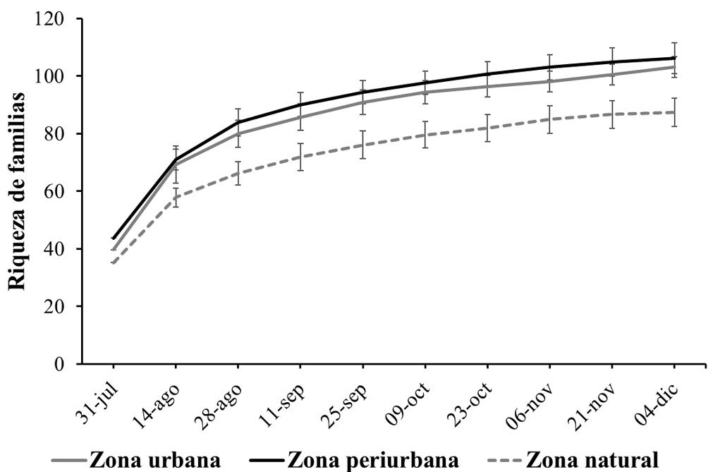
Discusión
Los resultados de este trabajo fueron contrarios a nuestra hipótesis de investigación, ya que ésta sugiere que en zonas con altos niveles de perturbación como las ciudades, habría menor diversidad de insectos, principalmente especialistas como los parasitoides, considerando la hipótesis del aumento del disturbio, que indica una disminución en la riqueza de artrópodos, particularmente especialistas, conforme aumenta el grado de urbanización (Gray, 1989, en Fenoglio et al., 2020) y la teoría sobre la complejidad estructural de la vegetación, que afirma que a mayor cobertura vegetal en ecosistemas, habrá un mayor número de plantas disponibles, lo que permitirá alojar mayor diversidad de fitófagos y, por consiguiente, de depredadores y parasitoides (González-Moreno et al., 2023; Guo et al., 2021; Neal et al., 2024).

Tabla 3
Diversidad verdadera de grupos funcionales de insectos, como número efectivo de familias, con números de Hill para estimar la riqueza de familias (0D), la diversidad de familias comunes (1D) y la diversidad de familias dominantes (2D) en 3 zonas con diferente nivel de perturbación de Yucatán. *Los intervalos de confianza (IDC) al 95%, indican diferencias significativas.
| Grupos funcionales | Índices de diversidad verdadera | ||
| 0D (95% IDC) | 1D (95% IDC) | 2D (95% IDC) | |
| Fitófagos | |||
| Zona urbana | 50.6 (39.9, 84.8) | 4.8 (4.6, 4.9)* | 3.2 (2.4, 4.1) |
| Zona periurbana | 42.4 (39.0, 56.7) | 7.2 (6.9, 7.4)* | 4.7 (4.0, 5.3) |
| Zona natural | 30.3 (27.7, 43.1) | 5.3 (5.0, 5.6)* | 3.1 (2.5, 3.8) |
| Polinizadores | |||
| Zona urbana | 14.9 (14.1, 25.2) | 6.7 (6.2, 7.2)* | 4.6 (4.2, 5.0) |
| Zona periurbana | 13.0 (13.0, 13.0) | 5.2 (5.0, 5.4)* | 3.7 (3.1, 4.3) |
| Zona natural | 12.5 (12.0, 20.0) | 4.4 (4.2, 4.7)* | 2.9 (2.3, 3.6) |
| Parasitoides | |||
| Zona urbana | 21.0 (21.0, 21.0) | 10.8 (10.0, 11.6)* | 7.7 (7.4, 8.0)* |
| Zona periurbana | 23.6 (22.3, 32.0) | 4.0 (3.6, 4.3)* | 2.3 (1.5, 3.1)* |
| Zona natural | 21.3 (20.2, 29.3) | 6.9 (6.0, 7.8)* | 4.2 (3.6, 4.8)* |
| Depredadores | |||
| Zona urbana | 18.7 (16.4, 31.7) | 4.1 (3.8, 4.5)* | 2.8 (2.0, 3.6)* |
| Zona periurbana | 17.5 (17.0, 22.7) | 7.0 (6.3, 7.7) | 5.0 (4.5, 5.6) |
Las diferencias encontradas en la riqueza de familias de insectos, sin tomar en cuenta su función en los ecosistemas, puede explicarse según la hipótesis de la perturbación media, que propone que la diversidad puede ser mayor en sitios donde la perturbación no es muy frecuente ni muy intensa, comparada con sitios no perturbados o con perturbación intensa (Connell, 1978).
El efecto de la perturbación y heterogeneidad del paisaje sobre la diversidad puede ser diferente dependiendo de la escala de estudio (Corcos et al., 2019), del taxón y del grupo funcional (Fenoglio et al., 2020), como se pudo observar en este trabajo. Las comunidades más diversas de fitófagos se presentaron en los sitios periurbanos con cultivos de maíz, probablemente, por la oferta mayor de alimento que puede representar el cultivo, facilitando el acceso a recursos alimenticios y refugio, que a su vez, favorece una mayor equidad de familias comunes (Landry et al., 2020); además, si consideramos nuevamente la hipótesis del disturbio medio, los sitios periurbanos con un nivel medio de perturbación, estarían alojando mayor diversidad, en este caso de fitófagos. Asimismo, se ha demostrado que zonas perturbadas que integran espacios verdes como parques urbanos, jardines residenciales, huertos verticales y familiares, parcelas de policultivos y parches de vegetación natural, favorecen la diversidad de fitófagos, al proporcionarles recursos alimenticios y refugios suficientes, que les permite adaptarse y prosperar en hábitats alterados por la actividad humana (Landry et al., 2020; Ruiz-Montoya et al., 2014). En los ensambles, la familia Pyralidae fue dominante en las zonas periurbana y natural, debido a su capacidad para aprovechar tanto plantas cultivadas como nativas, lo que le permite alimentarse y completar su ciclo de vida con eficacia (Cepeda, 2017). En cambio, las comunidades de la zona urbana estuvieron dominadas por la familia Cicadellidae, lo que refleja su adaptación a ambientes con altos niveles de perturbación (Trivellone et al., 2021).
La mayor diversidad de polinizadores en ciudad puede estar relacionada con la variabilidad y abundancia de recursos florales de los jardines, parques y áreas verdes presentes en los sitios, al proporcionar ciertas fuentes polínicas que favorecen dicha diversidad; estos resultados son contrarios a la que esperábamos si se considera la teoría sobre el espectro de polinización, que afirma, que a mayor cobertura vegetal en los ecosistemas, habrá un mayor número de plantas con flores, lo que permitirá alojar mayor diversidad de polinizadores. Sin embargo, es importante señalar que esta diversidad estuvo representada por familias de lepidópteros y no por abejas, debido probablemente a que estas últimas son de los grupos más sensibles a la contaminación de las ciudades (Roguz et al., 2023). Aunque se ha demostrado que en áreas urbanas, cuando se crean nuevos hábitats o refugios, como hoteles para polinizadores, jardines florales y corredores de flores silvestres, la diversidad de polinizadores tiende a incrementarse (Francini et al., 2022; Persson et al., 2023); pero el grupo de polinizadores varía dependiendo de ciertos factores asociados a la urbanización, por ejemplo, los abejorros son muy sensibles a la contaminación de las ciudades (Roguz et al., 2023); pero otros grupos pueden tener la capacidad de alimentarse en entornos urbanos (McLeod et al., 2021), como las mariposas (Lepidoptera: Papilionoidea) que son más tolerantes a la urbanización que otros polinizadores como sírfidos, moscas abejorros (Diptera: Syrphidae, Bombyliidae) y abejas (Hymenoptera: Apoidea) (Ávalos-Hernández et al., 2024). Es importante señalar que la diversidad observada es de familias consideradas comunes, lo que está reflejando la adaptación de ciertos polinizadores generalistas, que se adaptan rápidamente a las condiciones altamente perturbadas y son capaces de aprovechar la oferta floral de estos sitios (Deguines et al., 2016; Neumann et al., 2024). Las familias dominantes encontradas en este trabajo se han registrado interactuando con varias especies de plantas en jardines urbanos, realizando la función de polinización (Wonderlin et al., 2019). Geometridae fue dominante en los huertos periurbanos con maíz, probablemente porque son lepidópteros que disminuyen en sitios más urbanizados (Gaona et al., 2021); Nymphalidae fue dominante en la vegetación natural y Erebidae en la ciudad; esto es relevante porque las áreas urbanas y agrícolas alteran los patrones de comportamiento de los lepidópteros nocturnos debido a la luz artificial, mientras que los lepidópteros diurnos en áreas naturales reflejan su dependencia de hábitats con bajo impacto humano (Seymoure, 2018).
La diversidad de parasitoides encontrada, también fue contraria a los patrones esperados, ya que, a mayor cobertura vegetal en los ecosistemas, habrá un mayor número de hospederos disponibles, lo que permitirá alojar mayor diversidad de parasitoides (Parsons y Frank, 2019). Esto puede explicarse por la denso-dependencia de los parasitoides a sus hospederos, incluso en ciudades (Rocha y Fellowes, 2018), probablemente, porque las trampas se colocaron en jardines de casas particulares, los cuales tenían diferentes especies vegetales, ornamentales, frutales y arbustivas que ofrecían microhábitats y recursos alimenticios a los hospederos y por consiguiente a sus parasitoides (Klaus et al., 2024; Lucatero et al., 2024; Start et al., 2020). Otra razón de los valores elevados de diversidad en la zona urbana, puede explicarse por la habilidad de dispersión de los bracónidos, ya que se ha comprobado que los artrópodos que ocupan altos niveles tróficos como depredadores y parasitoides, serán exitosos en sitios urbanos, si tienen alta capacidad de dispersión (Korányi et al., 2022). Tachinidae, que no ha sido registrada como una familia particularmente abundante para la región, fue dominante en los huertos periurbanos con maíz y la vegetación natural; además no es una familia de parasitoides hiperdiversa en comparación con los himenópteros parasitoides, por lo que es menos probable de encontrarse como dominante en los sitios (Kankonda et al., 2018). Por otra parte, se ha registrado que la abundancia de esta familia disminuye en áreas con altas densidades de edificios y calles que actúan como barreras que dificultan la dispersión de los individuos, así como la localización de sus hospederos (Corcos et al., 2019). Por el contrario, la familia Braconidae dominó los sitios de zonas urbanas, lo que podría sugerir su adaptación a ambientes altamente perturbados (Koptur et al., 2024), además de que se ha demostrado que la urbanización favorece especies generalistas capaces de explotar diferentes recursos, como podría ser el caso de Braconidae, parasitoides con mayor variedad en estrategias de desarrollo y biología.
Los depredadores fueron más diversos en áreas periurbanas con maíz y selva, al contrario de los parasitoides, que fueron más diversos en ciudad, probablemente porque al ocupar nichos similares, estén evitando la competencia. Cabe destacar que los depredadores, estuvieron representados mayoritariamente por diferentes familias del orden Coleoptera, que es uno de los grupos de insectos más afectados por la urbanización en términos de riqueza de especies, pero no de abundancia (Fenoglio et al., 2020). Aunque los coleópteros depredadores pueden aprovechar más eficientemente la oferta extendida del alimento que otros enemigos naturales, al adaptarse mejor a los cambios ambientales por urbanización (Gardiner et al., 2021; Liere y Cowal, 2024); como se observó en nuestros resultados, Coccinellidae fue dominante únicamente en la zona urbana, lo que confirma que son los depredadores mejor adaptados a la urbanización, por su capacidad para prosperar en las condiciones microclimáticas características de este ambiente (Kawakami et al., 2016; Meseguer et al., 2024). En cambio, Asilidae fue dominante en las zonas periurbana con maíz y natural, lo que puede reflejar su mayor supervivencia en zonas menos modificadas por la actividad humana (Pascacio-Villafán y Cohen, 2023).
Las diferencias de diversidad observadas para los diferentes ensambles de insectos, reflejan que las zonas urbanas pueden inducir cambios en las comunidades de insectos, e incluso, en algunos casos, favorecer esta diversidad. Pero, esto solo funcionará para cierto grupo de organismos que tengan estrategias tipo “r”, con hábitos generalistas y alta capacidad de dispersión y adaptación, que los hace exitosos en ambientes urbanos (Martinson y Raupp, 2013), como ciertas especies de avispas que pueden ser resistentes a la urbanización (Christie y Hochuli, 2009), como en nuestros resultados representadas por Braconidae; también familias que estén mejor adaptadas a ambientes con altos niveles de perturbación y que pueden colonizar nuevos hábitats creados por la actividad humana y volverse dominantes dentro de las comunidades al verse favorecidas por factores ambientales como la temperatura y la humedad (Adams et al., 2020; Sire et al., 2022). Sin embargo, los resultados contrastantes reportados en la literatura sobre los efectos de la urbanización sobre las comunidades de artrópodos (Arnold, 2022), sugieren que es prioritario continuar con esta línea de investigación.
En conclusión, la riqueza de insectos en sitios con distintos niveles de perturbación fue similar; sin embargo, se encontraron diferencias en la diversidad de familias comunes, esto resulta relevante debido a que los análisis se realizaron a un nivel taxonómico alto, de familia, donde normalmente es difícil detectar variaciones significativas en diversidad. Cabe destacar, que las diferencias fueron con las familias consideradas comunes, que probablemente sean las que presentan biologías generalistas que les permite adaptarse a condiciones adversas como las que existen en zonas perturbadas.
Contrario a lo esperado, la mayor diversidad de insectos no se encontró en la vegetación natural, sino que fue en los sitios periurbanos con cultivos de maíz, con niveles de perturbación moderados, con la familia Pyralidae dominando las comunidades. En la zona urbana, con el mayor grado de perturbación, los grupos de insectos más diversos fueron parasitoides y polinizadores con las familias Tachinidae y Erebidae, representando la dominancia de cada grupo funcional, respectivamente. Por el contrario, en la zona de menor perturbación, como fue la vegetación natural, únicamente los depredadores presentaron la mayor diversidad de insectos, con la familia Asilidae como dominante.
Agradecimientos
Los autores agradecen al Tecnológico Nacional de México por el financiamiento del proyecto “Huertos familiares y conservación de la diversidad de entomofauna benéfica” (clave: 20070.24-P) y al Consejo Nacional de Humanidades, Ciencia y Tecnología por la beca de posgrado otorgada al primer autor. También agradecemos a Xiomara Gálvez Aguilera, directora de la asociación Caribbean Conservation Coastal Ecosistem A.C., por permitirnos el acceso a la reserva privada “Komchen de los pájaros”.
Referencias
Adams, B. J., Li, E., Bahlai, C. A., Meineke, E. K., McGlynn, T. P. y Brown, B. V. (2020). Local and landscape scale variables shape insect diversity in an urban biodiversity hotspot. Ecological Applications, 30, e02089. https://doi.org/10.1002/eap.2089
Ávalos-Hernández, O., Trujano-Ortega, M., Ortega-Álvarez, R., Martínez-Fuentes, R. G., Calderón-Parra, R., García-Luna, F. et al. (2024). How does urbanization affect the fauna of the largest urban forest in Mexico? Urban Forestry and Urban Greening, 92, 128191. https://doi.org/10.1016/j.ufug.2023.128191
Arnold, J.E. (2022). Biological control services from parasitic Hymenoptera in urban agriculture. Insects, 13, 467. https://doi.org/10.3390/insects13050467
Arnett Jr., R. H. (2000). American insects: a handbook of the insects of America North of Mexico. Boca Ratón, Florida: CRC Press. https://doi.org/10.1201/9781482273892
Betancourt, E. O. M., Batis, B. V., Quiala, A. P., García, Y. M. R., Madariaga, M. C. y González, R. M. (2021). Diversidad de insectos benéficos asociada a la flora existente en fincas suburbanas en Santiago de Cuba, Cuba. Revista Chilena de Entomología, 47, 121–145. https://doi.org/10.35249/rche.47.1.21.13
Betts, M. G., Wolf, C., Pfeifer, M., Banks-Leite, C., Arroyo-Rodríguez, V., Ribeiro, D. B. et al. (2019). Extinction filters mediate the global effects of habitat fragmentation on animals. Science, 366, 1236–1239. https://doi.org/10.1126/science.aax9387
Biella, P., Tommasi, N., Guzzetti, L., Pioltelli, E., Labra, M. y Galimberti, A. (2022). City climate and landscape structure shape pollinators, nectar and transported pollen along a gradient of urbanization. Journal of Applied Ecology, 59, 1586–1595. https://doi.org/10.1111/1365-2664.14168
Biles, J. J. y Lemberg, D. S. (2023). A multi-scale analysis of urban warming in residential areas of a Latin American city: the case of Mérida, Mexico. Journal of Planning Education and Research, 43, 881–896. https://doi.org/10.1177/0739456X20923002
Borror, D. J. y White, R. E. (1998). A field guide to insects: America North of Mexico (Peterson field guides). Boston: Houghton Mifflin Harcourt.
Boyes, D. H., Evans, D. M., Fox, R., Parsons, M. S. y Pocock, M. J. (2021). Is light pollution driving moth population declines? A review of causal mechanisms across the life cycle. Insect Conservation and Diversity, 14, 167–187. https://doi.org/10.1111/icad.12447
Cepeda, D. E. (2017). Introducción a los Phycitinae de Chile (Lepidoptera: Pyralidae), nuevo registro y descripción de una nueva especie del género Homoeographa Ragonot, 1888. Insecta Mundi, 556, 1–9.
Chan-Canché, R., Ballina-Gómez, H., Leirana-Alcocer, J., Bordera, S. y González-Moreno, A. (2020). Sampling of parasitoid Hymenoptera: influence of the height on the ground. Journal of Hymenoptera Research, 78, 19–31. https://doi.org/10.3897/jhr.78.54309
Chao, A. y Shen, T.J. (2010). User’s guide for program SPADE (Species Prediction and Diversity Estimation). Taiwan: National Tsing Hua University.
Christie, F. J. y Hochuli, D. F. (2009). Responses of wasp communities to urbanization: effects on community resilience and species diversity. Journal of Insect Conservation, 13, 213–221. https://doi.org/10.1007/s10841-008-9146-5
Colwell, R. K. (2006). EstimateS: statistical estimation of species richness and shared species from samples. Versión 8 [consultado 18 Abr 2025]. Recuperado de: http://purl.oclc.org/estimates
Colwell, R. K. y Elsensohn, J. E. (2014). EstimateS turns 20: Statistical estimation of species richness and shared species from samples, with non parametric extrapolation. Ecography, 37, 609–613.
Connell, J. (1978). Diversity in tropical rain forests and coral reefs. Science, 199, 1304–1310. https://doi.org/10.1126/science.199.4335.1302
Corcos, D., Cerretti, P., Caruso, V., Mei, M., Falco, M. y Marini, L. (2019). Impact of urbanization on predator and parasitoid insects at multiple spatial scales. Plos One, 14, e0214068. https://doi.org/10.1371/journal.pone.0214068
Cortés-Arzola, S. V. y León-Cortés, J. L. (2021). Response of beetle assemblages (Insecta: Coleoptera) to patch characteristics and habitat complexity in an ever-expanding urban landscape in the Yucatán Peninsula, Mexico. Annals of the Entomological Society of America, 114, 511–521. https://doi.org/10.1093/aesa/saab017
Deguines, N., Julliard, R., De Flores, M. y Fontaine, C. (2016). Functional homogenization of flower visitor communities with urbanization. Ecology and Evolution, 6, 1967–1976. https://doi.org/10.1002/ece3.2009
Dirzo, R., Young, H. S., Galetti, M., Ceballos, G., Isaac, N. J. y Collen, B. (2014). Defaunation in the Anthropocene. Science, 345, 401–406. https://doi.org/10.1126/science.1251817
Fahrig, L., Arroyo-Rodríguez, V., Bennett, J. R., Boucher-Lalonde, V., Cazetta, E., Currie, D. J. et al. (2019). Is habitat fragmentation bad for biodiversity? Biological Conservation, 230, 179–186. https://doi.org/10.1016/j.biocon.2018.12.026
Fenoglio, M. S., Rossetti, M. R. y Videla, M. (2020). Negative effects of urbanization on terrestrial arthropod communities: a meta-analysis. Global Ecology and Biogeography, 29, 1412–1429. https://doi.org/10.1111/geb.13107
Fisogni, A., Hautekèete, N., Piquot, Y., Brun, M., Vanappelghem, C., Michez, D. et al. (2020). Urbanization drives an early spring for plants but not for pollinators. Oikos, 129, 1681–1691. https://doi.org/10.1111/oik.07274
Flores, J. S. y Espejel, I. (1994). Tipos de vegetación de la Península de Yucatán. Etnoflora yucatanense, Fascículo 3. Mérida: Universidad Autónoma de Yucatán.
Francini, A., Romano, D., Toscano, S. y Ferrante, A. (2022). The contribution of ornamental plants to urban ecosystem services. Earth, 3, 1258–1274. https://doi.org/10.3390/earth
3040071
Gaona, F. P., Íñiguez-Armijos, C., Brehm, G., Fiedler, K. y Espinosa, C. I. (2021). Drastic loss of insects (Lepidoptera: Geometridae) in urban landscapes in a tropical biodiversity hotspot. Journal of Insect Conservation, 25, 395–405. https://doi.org/10.1007/s10841-021-00308-9
Gardiner, M. M., Perry, K. I., Riley, C. B., Turo, K. J., Delgado-de la Flor, Y. A. y Sivakoff, F. S. (2021). Community science data suggests that urbanization and forest habitat loss threaten aphidophagous native lady beetles. Ecology and Evolution, 11, 2761–2774. https://doi.org/10.1002/ece3.7229
González-Moreno, A., Bordera, S., Ballina-Gómez, H. y Leirana-Alcocer, J. (2023). Age matters: variations in parasitoid diversity along a successional gradient in a dry semi-deciduous tropical forest. Bulletin of Entomological Research, 113, 604–614. https://doi.org/10.1017/S0007485323000287
Goulet, H. y Huber, J. T. (1993). Hymenoptera of the World: an identification guide to families. Ottawa: Agriculture Canada, Research Branch.
Guo, P. F., Wang, M. Q., Orr, M., Li, Y., Chen, J.T., Zhou, Q. S. et al. (2021). Tree diversity promotes predatory wasps and parasitoids but not pollinator bees in a subtropical experimental forest. Basic and Applied Ecology, 53, 134–142. https://doi.org/10.1016/j.baae.2021.03.007
Janzen, D. H. y Hallwachs, W. (2021). To us insectometers, it is clear that insect decline in our Costa Rican tropics is real, so let’s be kind to the survivors. Proceedings of the National Academy of Sciences, 118, e2002546117. https://doi.org/10.1073/pnas.2002546117
Jost, L. (2006). Entropy and diversity. Oikos, 113, 363–375. https://doi.org/10.1111/j.2006.0030-1299.14714.x
Kaczmarek, M., Entling, M. H. y Hoffmann, C. (2022). Using malaise traps and metabarcoding for biodiversity assessment in vineyards: Effects of weather and trapping effort. Insects, 13, 507. https://doi.org/10.3390/insects13060507
Kankonda, O. M., Akaibe, B. D., Sylvain, N. M. y Le Ru, B. P. (2018). Response of maize stemborers and associated parasitoids to the spread of grasses in the rainforest zone of Kisangani, DR Congo: effect on stemborers biological control. Agricultural and Forest Entomology, 20, 150–161. https://doi.org/10.1111/afe.12238
Kawakami, Y., Yamazaki, K. y Ohashi, K. (2016). Population dynamics, seasonality and aphid prey of Cheilomenes sexmaculata (Coleoptera: Coccinellidae) in an urban park in central Japan. European Journal of Entomology, 113, 192–199. https://doi.org/10.14411/eje.2016.023
Klaus, F., Tscharntke, T. y Grass, I. (2024). Trophic level and specialization moderate effects of habitat loss and land-
scape diversity on cavity nesting bees, wasps, and their parasitoids. Insect Conservation and Diversity, 17, 65–76. https://doi.org/10.1111/icad.12688
Koptur, S., Primoli, A. S., Paulino-Neto, H. F. y Whitfield, J. (2024). Pierid butterflies, legume hostplants, and parasitoids in urban areas of Southern Florida. Insects, 15, 123. https://doi.org/10.3390/insects15020123
Korányi, D., Egerer, M., Rusch, A., Szabó, B. y Batáry, P. (2022). Urbanization hampers biological control of insect pests: a global meta-analysis. Science of the Total Environment, 834, 155396. https://doi.org/10.1016/j.scitotenv.2022.155396
Landry, B., Basset, Y., Hebert, P. D. y Maes, J. M. (2020). On the Pyraloidea fauna of Nicaragua. Tropical Lepidoptera Research, 30, 93–102.
Liere, H. y Cowal, S. (2024). Local and landscape factors differentially influence predatory arthropods in urban agroecosystems. Ecosphere, 15, e4816. https://doi.org/10.
1002/ecs2.4816
Lucatero, A., Smith, N. R., Bichier, P., Liere, H. y Philpott, S. M. (2024). Shifts in host–parasitoid networks across community garden management and urban landscape gradients. Ecosphere, 15, e4833. https://doi.org/10.1002/ecs2.4833
Magurran, A. E. (2004). Measuring biological diversity. Oxford: Blackwell Publishing.
Martínez-Ramos, M., Pingarroni, A., Rodríguez-Velázquez, J., Toledo-Chelala, L., Zermeño-Hernández, I. y Bongers, F. (2016). Natural forest regeneration and ecological restoration in human modified tropical landscapes. Biotropica, 48, 745–757. https://doi.org/10.1111/btp.12382
Martinson, H. M. y Raupp, M. J. (2013). A meta-analysis of the effects of urbanisation on ground beetle communities. Ecosphere, 4, 1–24. https://doi.org/10.1890/ES12-00262.1
Martorell, C. y Peters, E. M. (2005). The measurement of chronic disturbance and its effects on the threatened cactus Mammillaria pectinifera. Biological Conservation, 124, 199–207. https://doi.org/10.1016/j.biocon.2005.01.025
Mc Leod, B. C., Águila, M. K., Zegers, M. G. y Cárcamo, G. J. (2021). Refugio u “Hoteles de Insectos”, simulación de hábitat para el establecimiento de fauna auxiliar. Punta Arenas, Chile: Informativo INIA Kampenaike. Núm. 110. Recuperado el 15 de enero, 2025 de: https://hdl.handle.net/20.500.14001/67359
Meseguer, R., Madeira, F., Kavallieratos, N. G. y Pons, X. (2024). Phenology, population trends and natural enemy complex of Illinoia liriodendri in Spain. Phytoparasitica, 52, 40. https://doi.org/10.1007/s12600-024-01145-7
Moreno, C. E., Barragán, F., Pineda, E. y Pavón, N. P. (2011). Reanálisis de la diversidad alfa: alternativas para interpretar y comparar información sobre comunidades ecológicas. Revista Mexicana de Biodiversidad, 82, 1249–1261. https://doi.org/10.22201/ib.20078706e.2011.4.745
Muñoz-Urias, A., Araujo-Alanis, L., Huerta-Martínez, F. M., Jacobo-Pereira, C. y Razo-León, A. E. (2025). Effects of urbanization and floral diversity on the bee community (Hymenoptera, Apoidea) in an oak forest in a Protected Natural Area of Mexico. Journal of Hymenoptera Research, 98, 47–68. https://doi.org/10.3897/jhr.98.131191
Neal, W., Araya, Y. y Wheeler, P. M. (2024). Influence of canopy structural complexity on urban woodland butterfly species richness. Journal of Insect Conservation, 28, 1051–1062. https://doi.org/10.1007/s10841-024-00594-z
Neumann, A. E., Conitz, F., Karlebowski, S., Sturm, U., Schmack, J. M. y Egerer, M. (2024). Flower richness is key to pollinator abundance: the role of garden features in cities. Basic and Applied Ecology, 79, 102–113. https://doi.org/10.1016/j.baae.2024.06.004
Parsons, S. E. y Frank, S. D. (2019). Urban tree pests and natural enemies respond to habitat at different spatial scales. Journal of Urban Ecology, 5, juz010. https://doi.org/10.1093/jue/juz010
Pascacio-Villafán, C. y Cohen, A. C. (2023). How rearing systems for various species of flies benefit humanity. Insects, 14, 553. https://doi.org/10.3390/insects14060553
Persson, A. S., Hederström, V., Ljungkvist, I., Nilsson, L. y Kendall, L. (2023). Citizen science initiatives increase pollinator activity in private gardens and green spaces. Frontiers in Sustainable Cities, 4, 1099100. https://doi.org/10.3389/frsc.2022.1099100
Ramírez-Restrepo, L. R. y Halffter, G. (2013). Butterfly diversity in a regional urbanization mosaic in two Mexican cities. Landscape and Urban Planning, 115, 39–48.
https://doi.org/10.1016/j.landurbplan.2013.03.005
Rocha, E. A. y Fellowes, M. D. E. (2018). Does urbanization explain differences in interactions between an insect herbivore and its natural enemies and mutualists? Urban Ecosystems, 21, 405–417. https://doi.org/10.1007/s11252-017-0727-5
Rocha-Ortega, M. y Castaño-Meneses, G. (2015). Effects of urbanization on the diversity of ant assemblages in tropical dry forests, Mexico. Urban ecosystems, 18, 1373–1388. https://doi.org/10.1007/s11252-015-0446-8
Roguz, K., Chiliński, M., Roguz, A. y Zych, M. (2023). Pollination of urban meadows. Plant reproductive success and urban-related factors influencing frequency of pollinators visits. Urban Forestry and Urban Greening, 84, 127944. https://doi.org/10.1016/j.ufug.2023.127944
Ruiz-Montoya, L., Alias, V. L. A., Alias, V. D. J., Guillén, D. T. A. y de la Mora, E. L. F. (2014). Diversidad y distribución de familias de insectos en el Cerrito de San Cristóbal. En L.Ruiz-Montoya (Coord.), Diversidad biológica y enriquecimiento florístico del Cerrito de San Cristóbal (pp. 39–56). El Colegio de la Frontera Sur.
Rzedowski, J. (1978). Vegetación de México. México D.F.: Limusa.
Schmidt, O., Schmidt S., Häuser, C., Hausmann, A. y Van Vu, L. (2019). Using Malaise traps for collecting Lepidoptera (Insecta), with notes on the preparation of Macrolepidoptera from ethanol. Biodiversity Data Journal, 7, e32192. https://doi.org/10.3897/BDJ.7.e32192
Seymoure, B. M. (2018). Enlightening butterfly conservation efforts: the importance of natural lighting for butterfly behavioral ecology and conservation. Insects, 9, 22. https://doi.org/10.3390/insects9010022
Sire, L., Yáñez, P. S., Wang, C., Bézier, A., Courtial, B., Cours, J. et al. (2022). Climate-induced forest dieback drives compositional changes in insect communities that are more pronounced for rare species. Communications Biology, 5, 57. https://doi.org/10.1038/s42003-021-02968-4
Start, D., Barbour, M. A. y Bonner, C. (2020). Urbanization reshapes a food web. Journal of Animal Ecology, 89, 808–816. https://doi.org/10.1111/1365-2656.13136
Tavares-Brancher, K. P., Graf, L. V., Ferreira-Júnior, W. G., Faria, L. D. B. y Zenni, R. D. (2024). Plant-pollinator interactions in the neotropics are affected by urbanization and the invasive bee Apis mellifera. Journal of Insect Conservation, 28, 251–261. https://doi.org/10.1007/s10841-024-00547-6
Triplehorn, C. A. y Johnson, N. F. (2005). Borror and Delong’s introduction to the study of insects. 7th Edition. Independence, KY: Cengage Learning.
Trivellone, V., Forte, V., Filippin, L. y Dietrich, C. H. (2021). First records of the North American leafhopper Gyponana mali (Hemiptera: Cicadellidae) invading urban gardens and agroecosystems in Europe. Acta Entomologica Musei Nationalis Pragae, 61, 213–219. https://doi.org/10.37520/aemnp.2021.011
Vergnes, A, Pellissier, V, Lemperiere, G, Rollard, C. y Clergeau, P. (2014). Urban densification causes the decline of ground-dwelling arthropods. Biodiversity and Conservation, 23, 1859–1877. https://doi.org/10. 1007/s10531-014-0689-3
Wagner, D. L., Grames, E. M., Forister, M. L., Berenbaum, M. R. y Stopak, D. (2021). Insect decline in the Anthropocene: Death by a thousand cuts. Proceedings of the National Academy of Sciences, 118, e2023989118. https://doi.org/10.1073/pnas.2023989118
Whittaker, R. H. (1972). Evolution and measurement of species diversity. Taxon, 21, 213–251. https://doi.org/10.2307/1218190
Wonderlin, N. E., Rumfelt, K. y White, P. J. (2019). Associations between nocturnal moths and flowers in urban gardens: evidence from pollen on moths. The Journal of the Lepidopterists’ Society, 73, 173–176. https://doi.org/10.18473/lepi.73i3.a6

Citizen science suggests decreased diversity of insects in Mexico, a megadiverse country
Datos de ciencia ciudadana sugieren un decremento en la diversidad de insectos de México, país megadiverso
Jorge Soberon *
University of Kansas, Biodiversity Institute, Dyche Hall, 1345 Jayhawk Blvd, Lawrence, KS 66045, USA
*Corresponding author: jsoberon@ku.edu (J. Soberon)
Received: 09 July 2025; accepted: 26 August 2025
Abstract
An analysis of iNaturalist data on several taxonomic groups of insects in Mexico is presented. A decreasing trend was observed in species diversity per year for 4 families of butterflies, bumblebees, and dragonflies and damselflies. Analyses were performed on several potential vegetation types (sensu Rzedowsky), and the roles of deforestation and pesticide use on the identified trends were explored. Challenges in using unsystematic data to estimate trends are discussed, and several hypotheses are provided to explain the results.
Keywords: Butterflies; Bumblebees; Damselflies; Dragonflies, iNaturalist
Resumen
Se presenta un análisis de datos de iNaturalist sobre varios grupos taxonómicos de insectos en México. Se observó una tendencia decreciente en la diversidad de especies por año para 4 familias de mariposas, y para abejorros y libélulas. Se realizaron análisis sobre varios tipos potenciales de vegetación (sensu Rzedowsky) y se exploró el papel de la deforestación y el uso de pesticidas en las tendencias identificadas. Se discuten los desafíos del uso de datos no sistemáticos para estimar tendencias y se presentan varias hipótesis para explicar los resultados.
Palabras clave: Mariposas, Abejorros; Caballitos del diablo; Libélulas; NaturaLista
Introduction
Evidence indicates a decrease in insect populations in many countries (Edwards et al., 2025; Hallmann et al., 2017). This finding is worrisome for many reasons, including that insects are key components of ecosystems and provide societies with important ecosystem services, such as pollination (Potts et al., 2010). Moreover, insects have substantial but largely unappreciated cultural importance (Duffus et al., 2021), not only worldwide but particularly in countries such as Mexico, where insects have culinary uses (Ramos-Elorduy & Viejo-Montesinos, 2007), have been important for ancestral cultures (Beutelspacher, 1989), and have economic and societal value (Ayala et al., 2012; Rogel-Fajardo et al., 2011).
Most detailed evidence of the decline in insects has come from countries in temperate zones that have developed formal monitoring schemes (Streitberger et al., 2024; Thomas, 2005). In contrast, tropical regions are less well studied (Sánchez-Herrera et al., 2024), and the existing evidence is contradictory (Bonadies et al., 2024; Boyle et al., 2025; Wagner et al., 2021). For instance, studies on Hemiptera (Lucas et al., 2016) and on saturniid moths (Basset et al., 2017) have indicated no trends in Barro Colorado Island, Panama. Similarly, in Veracruz, Mexico, well monitored fruit flies have shown no trends (Aluja et al., 2012; Ordano et al., 2013). In contrast, decreases in saturniid larvae have been reported in Costa Rica (Salcido et al., 2020), and declines in arthropod biomass have been reported in Puerto Rico and, on the basis of a few data points, in Chamela, Mexico (Lister & García, 2018). The monarch butterfly, perhaps the best monitored insect species in Mexico, has shown consistent decreases in its wintering aggregations (Thogmartin et al., 2017; Vidal & Rendón-Salinas, 2014; Zylstra et al., 2021).
Because of its history, climate, topography, and cultural milieu (Ramamoorthy et al., 1993), Mexico is among the world’s megadiverse countries (Mittermeier et al., 1997). Therefore, assessing the trends in insect populations in Mexico should be prioritized. Unfortunately, long-term insect monitoring in Mexico is rare. Although Mexico has a long history of entomological research, including many collections and hundreds of publications (Michán & Llorente, 2002), monitoring has been limited to only a few species. Although the reasons for the lack of national monitoring schemes like those existing in other countries should be determined, this study does not attempt to do so. It takes as a premise that, in Mexico, just a few systematically obtained insect time series of more than 2-3 years long are available. This study is aimed at estimating insect biodiversity trends in Mexico, despite the absence of systematic monitoring efforts.
Systematic monitoring results are compiled in several worldwide time series databases, such as the Living Planet Index (Almond et al., 2020) and the Global Population Dynamics database (NERC Centre for Population Biology, 1999). Unfortunately, these databases have sparse insect information and contain no data for Mexico. Another possibility is using so-called citizen science (CS) data (Cohn, 2008), which, although opportunistic and unsystematic, is often abundant. Data on insects collected by non-professionals have been used to estimate phenology and distributions (Soroye et al., 2018). However, using such data to estimate population trends is challenging, as discussed below.
In Mexico, perhaps the most comprehensive CS initiative is iNaturalist (known as Naturalista in Mexico). iNaturalist began its operations in Mexico in 2008, although in 2013 the initiative came under the leadership of the national biodiversity agency, Conabio, under the name of Naturalista (Macías & Freire, 2017) and obtained funding from the Slim Foundation. Therefore, in Mexico, iNaturalist began in earnest in 2013. Despite this relatively late start, Mexico is the third country in amount of data (Mason et al., 2025) and it contains more than 80,000 records tagged as “research level” for 3 families of butterflies, and the damselflies, dragonflies, and bumblebees. This substantial information may be used to assess trends. However, CS data must be corrected for biases, of which are many (Crall et al., 2011). Specifically, in Mexico, the number of observers (and thus of observations) in iNaturalist increases each year (Table S1), and this bias should be considered when using such data.
Indeed, a major problem in using opportunistic CS data to estimate trends is correcting for biases in recording efforts (Di Cecco et al., 2021). Several methods can be used to address this problem (Isaac et al., 2014; Outhwaite, 2019; Tang et al., 2021). One of the simplest methods is correcting bias by obtaining the quotient of the metric used to report biodiversity to some measure of the effort invested in a locality, for a given period. What is “effort,” and how can it be measured in iNaturalist data? Collection effort is difficult to define but can be described in terms of: 1) the time spent collecting, 2) the method of collection and number of collectors, or 3) the number of specimens or species observed (Gulland, 1969; Willott, 2001). iNaturalist data allows for extraction of a measure of time (number of monthly observations in a year), but data quality (beyond the “research” tag, which refers to the reliability of the name assigned to the species), remains unreported, and worse, in the case of iNaturalist, this quality is known to change (Di Cecco et al., 2021). Di Cecco (2021) has suggested that, in iNaturalist, observers with at least 2 observations are more reliable than those with just 1 observation. Therefore, as a measure of effort, this study used the number of observers with 2 or more observations. As biodiversity measures it is used the number of species, and the number of observations, pooled for spatial units and year. Two indices are then calculated: number of species/effort, and number of records/effort.
Ordinary regressions of metrics against time often experience problems of autocorrelated errors and non-equal variances (heteroskedasticity). These are characteristic of time series (Shumway & Stoffer, 2005) and must be accounted for. One method of addressing the complexities of analysis of count time series data is using a package such as “trim” (in the R platform), which assumes a Poisson model for the underlying data (Pannekoek, 1998). This approach corrects for the autocorrelation of errors and for heteroskedasticity. Trim has frequently been used for European (van Strien et al., 2019) and tropical American (Novoyny & Basset, 2000) data, but the key assumption of count data (a discrete scale) complicates analysis of continuous-scale indices, or data including many non-occurrences, because the software is sensitive to the presence of zeroes, or NAs, in the data.
Another possibility is estimating whether a significant trend exists in the data, by using a non-parametric Mann-Kendall test (Lyubchich et al., 2013). An ordinary least squares linear regression (OLS) of metric against time is first performed, and the existence of trends (linear or monotonic) is subsequently determined. This method uses the sign of the slope in the OLS, and the significance is tested with the Mann-Kendall test.
Additional methods can be used, such as, for a single species, the logit of the probability of occupancy of a cell, on a time unit (van Strien et al., 2019) and fit a generalized linear model of predictors, by using the length of the list of species as a measure of effort (Szabo et al., 2010). Then several single species regressions can be combined in an index (van Strien et al., 2019). One problem with this approach is that generalized linear modeling is based on an assumption of independence of errors, which might be violated in a time series.
A statistically more sophisticated modification of the above idea is reporting the proportion of occupied sites under a hierarchical model that separates the actual presence from the act of observation (Outhwaite, 2019). Although apparently very rigorous, this approach has its own problems, including the need to define an appropriate model for the “present” and “observer” components, and the need to have replicated visits to the same site within the same season (van Strien et al., 2019).
Another possibility is using generalized least squares (GLS) regressions, which allow for autocorrelated errors and heteroskedasticity. The R package “nlme” implements this technique. This method can fit an ordinary regression of the index against covariates such as time, and another regression including autocorrelation with power variance decay in its model. Subsequently, the 2 models can be compared with the Akaike criterion, and the best model can be retained. This option was used here, with the simplest ARIMA model with lag = 1 as a model of correlated errors.
This study further assessed whether any existing trends might have differed for different ecological regions of Mexico. A variety of subdivisions of Mexico have been suggested, according to different ecological perspectives, at different spatial resolutions (Anonymous, 1997; Challenger & Soberón, 2012; Miranda & Hernández, 1963; Olson et al., 2001). Here, Rzedowsky’s potential vegetation types were used (Rzedowsky, 1986). Although coarse-grained, these types are based primarily on straightforward floristic criteria, are well known in Mexico, and have a small number of categories.
An important caveat in using CS data is that species that are difficult to identify by sight should be avoided. This work focused on 3 families of butterflies (Papilionidae, Pieridae, and Nymphalidae), with 316 names (skippers and the smallest families in the Papilionoidea were excluded); 23 names for bumblebees; and 293 names for the Odonata (both Zygoptera and Anysoptera). In addition, as a comparison, data on 307 names for Solanaceae were included. The numbers of names (without proper taxonomic validation by experts), as reported by iNaturalist, are listed in Table 1.
For the butterflies, although using species identified as indicators of “conservation” status (Orta et al., 2022) would have been interesting, most species identified by these authors as indicators had only a few records in the iNaturalist database. Therefore, the analysis was performed not by individual species, but by pooling all the data in the 3 families of butterflies, all the dragon and damselflies, and all the bumblebees.
For obtaining uncertainty bands, grids of hexagons covering the territory of Mexico were defined at several resolutions (Fig. 1). For a given year and taxonomic group, the means and variances over hexagons were determined. Each unique combination of year and hexagon defined an “event,” and thus the abundance metrics were: 1) the number of observations per event (cumulative monthly observations); and 2) the number of different species per event. As a measure of effort, the total number of different observers with at least 2 observations in each “event” was used. The final index was the average over all hexagons with at least 1 record, for a given year, of the number of observations or the number of species, per observer.
Table 1
Numbers of scientific names for the different taxonomic groups in the 4 most visited potential vegetation classes. The butterflies are the Papilionidae (swallowtails), Pieridae (sulfurs), and Nymphalidae (brushfoots).
| All Mexico | Xerophytic Shrub | Pine Oak Forest | Grasslands | Tropical Deciduous Forest | |
| Butterflies | 413 | 153 | 220 | 220 | 198 |
| Odonata | 292 | 185 | 187 | 105 | 184 |
| Bombus | 23 | 16 | 20 | 9 | 14 |
| Solanaceae | 307 | 176 | 210 | 111 | 153 |
Changing the hexagon area might potentially change the results. This problem, described as the “modifiable areal unit problem,” has been long known to geographers (Openshaw, 1984). Fortunately, in this case, the qualitative results were not affected by the resolution of the hexagons (data correlations among resolutions always exceeded 0.7). Consequently, only the analysis using the largest (2 degrees) hexagons (n = 81) is reported.
The literature has suggested that the decrease in insect abundance has been due to: 1) increased use of pesticides, 2) decreased habitat area (or increased transformed land area), and 3) climate change. At the scale of the whole country, regressions of data versus time series of pesticide use and deforestation rates are reported.
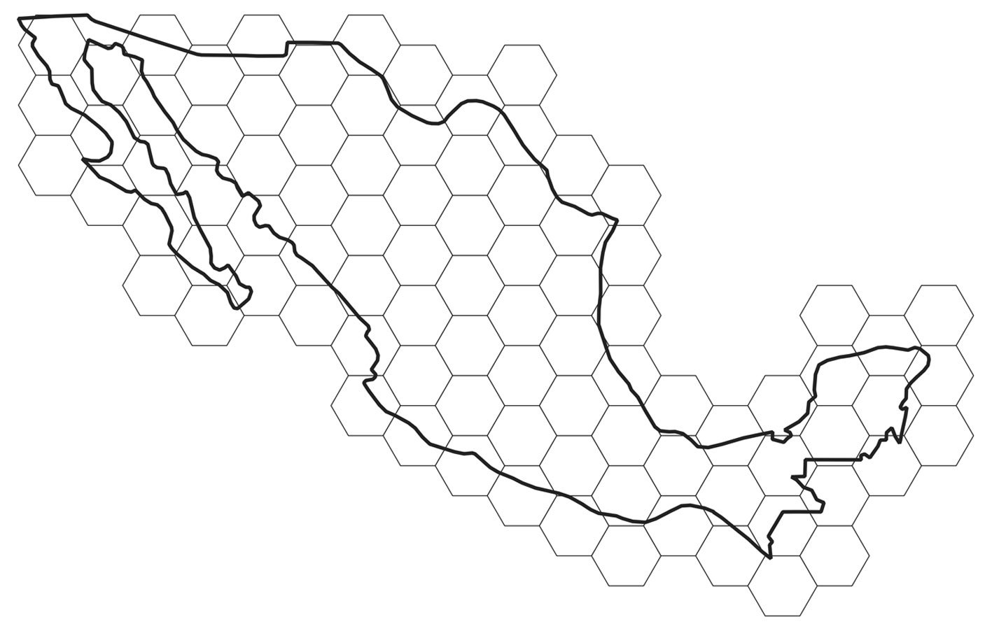
Materials and methods
CS data are not ideally suited to the estimation of trends, primarily because of the biased and uneven methods of sampling sites, times, and species. This work used 1 of the 3 methods proposed by Isaac et al. (2014): correcting the reported number of sightings according to a measure of effort. iNaturalist data were downloaded from the Global Biodiversity Information Network (GBIF), as detailed in Table 2.
Data were divided into subsets (keeping records with coordinates) for the 4 largest families in the Papilionoidea: Papilionidae (5,583 records), Pieridae (29,994 records), Nymphalidae (20,145 records), and Lycaenidae (2,326 records). The Lycaenidae was removed from the analysis because many species are relatively difficult to determine visually. Data for the genus Bombus (bumblebees, 6,543 records) and the 2 suborders of the Odonata (the Zygoptera, 12,772 records, and the Anisoptera, 24,003 records) were also downloaded. For comparison purposes, observations of the nightshade family, the Solanaceae (39,014 records), were downloaded. The number and positions of every observation in Mexico are presented in figure 2.
Table 2
Digital Object Identifiers (DOIs) from GBIF for the datasets used in the work.
| Taxon | GBIF DOI | iNaturalist Records | Unique names |
| Nymphalidae | doi.org/10.15468/dl.qta4zp | 20,145 | 223 |
| Papilionidae | doi.org/10.15468/dl.uu4unc | 5,583 | 13 |
| Pieridae | doi.org/10.15468/dl.zug4ee | 29,994 | 80 |
| Lycaenidae | doi.org/10.15468/dl.xgad6g | 2,326 | 97 |
| Odonata | doi.org/10.15468/dl.atdkfz | 36,775 | 292 |
| Anisoptera | 24,003 | 163 | |
| Zygoptera | 12,772 | 129 | |
| Bombus | doi.org/10.15468/dl.c6h4jz | 6,543 | 23 |
| Solanaceae | doi.org/10.15468/dl.597nj5 | 39,014 | 307 |
Data tagged as “research quality” in the downloaded GBIF data were retained, and basic data cleaning was performed to keep the coordinates inside Mexico. No attempt was made to correct for outdated taxonomy or other known issues present in aggregator data (Chapman, 2005).
Data can be organized as time series, by pooling the observations in a year. This method has a drawback of potentially missing seasonality; however, pooling by month produces tables that are too sparse and therefore are difficult to analyze. To include some measure of uncertainty in the trends, the averages of the calculated indices over all non-empty (i.e., with at least 1 observation) hexagons of 2 degrees of surface were determined, and its standard error calculated.
Two indices were used: different_species/observer and records/observer. The first is a measure of diversity, whereas the second is a measure of abundance. Findings for both are reported. “Observers” refers to the number of observers with at least 2 registered observations.
To summarize trends, a useful statistic may be the slope of a linear model of index as a function of time, which requires regressions of index vs. year. However, as previously discussed, the errors in many time series are not independent, and the equal variance assumption of ordinary least squares is also often violated. If uncorrec-
ted, these problems interfere with rigorous calculations of probability under a null hypothesis (McShane et al., 2019). Among the many methods for addressing this problem, generalized least squares regressions (Baillie & Kim, 2018), which enable inclusion of an autoregressive structure of correlations and violations of homoscedasticity, were chosen herein. Two models were fitted to the data: an ordinary linear least squares, and a first order auto-regressive, moving average model (ARIMA) (Shumway & Stoffer, 2005) allowing for heteroskedasticity. The 2 models were compared with an ANOVA (Fox & Weisberg, 2019), and the most likely model (based on the Akaike criterion; see Fox & Weisberg, 2019) was used. This process permitted to obtain, in a rigorous way, the probability for the observed slope values, under a null hypothesis of a slope equal to zero. Reporting the “significance” of slopes has been substantially criticized (McShane et al., 2019). Therefore, the probability (rather than the “significance”) of the slope, based on the assumption of a null model of no trend, is reported. Very small probabilities are highlighted.
The regressions included 2 possible causal factors: forest loss and use of pesticides. The deforestation rate was obtained from the Global Forest Watch website (Sims et al., 2024) with a threshold of 30% of forest cover, as recommended by Sims et al. (2024). This dataset has maintained methodological consistency (Hansen et al., 2013) and therefore is preferable to the INEGI Series (Gebhardt et al., 2015). Agrochemical use was determined as the amount of pesticides used per hectare of cropland, as reported on the FAO Web site. The data came from government reports https://www.fao.org/faostat/en/#data/RP. A discussion of the FAO dataset’s strengths and problems has been provided by Shattuck et al. (2023).
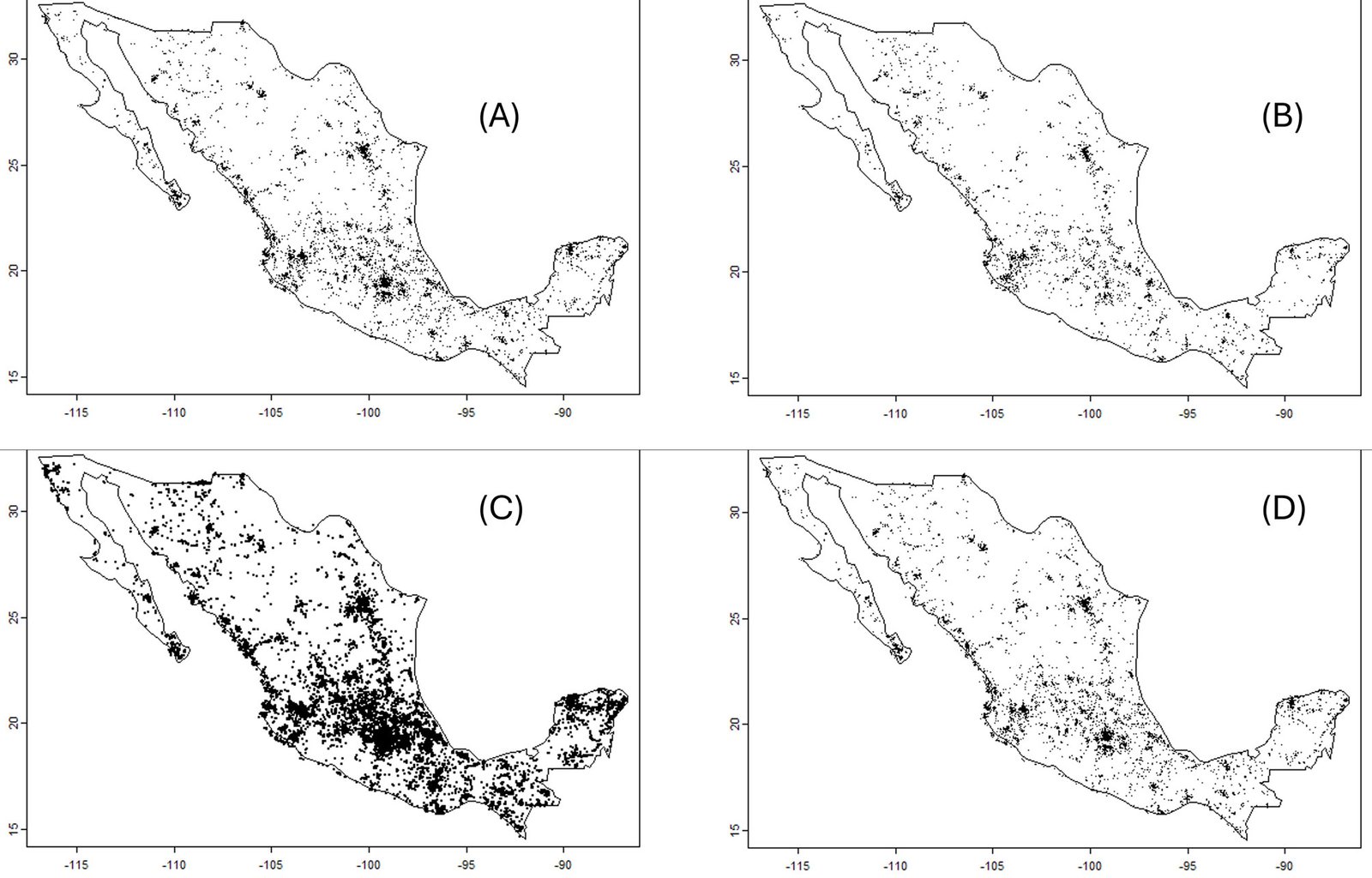
Because the probability of the observed values of the slope of the index of diversity per unit of effort vs. time, under a null hypothesis of 0 slope, was small in most cases, the regression was assumed to remove the time trend, and factors affecting just the residuals were searched for. That is, the residual of the index vs. time regressions was regressed against 2 predictors: deforestation rate and use of pesticides. The results are shown in the Supplementary materials.
To aggregate by “biome,” the subdivision of the Potential Vegetation of Mexico (Rzedowsky, 1986) was selected. A shapefile of Rzedowsky’s map at 1:4,000,000 scale, available at Conabio Geoportal, is produced by Instituto de Geografía, UNAM México. This map was used to pool the iNaturalist records according to potential vegetation, by using the 4 categories with the highest number of iNaturalist reports.
An informal survey was circulated among scientists working in 3 major ecology research centers in Mexico (INECOL, Veracruz, Instituto de Ecología, UNAM, and Ecosur, Chiapas). A total of 37 questionnaires were sent with Qualtrics. The questions are provided in the Supplementary materials. The main data tables and R code are openly available (Creative Commons CC0: 1) at https://github.com/jsoberon/iNaturalistInsectsMexico
Results
The informal questionnaire received 27 responses out of 37 requests. Among the respondents, 84% stated that they have observed a decrease in the number of insects either in streetlights in villages, or in the windshields or radiators of field vehicles. Although these answers lacked statistical rigor, they suggested a widespread perception among field biologists in Mexico that insect populations are becoming smaller.
The iNaturalist data provided a more nuanced picture. Before examining the trends in biodiversity indices, basic data were analyzed. Indeed, both the number of species and the number of observers (with more than 2 observations) increased (Fig. 3).
The numbers of observed species and observers both increase over time. The increased number of observers introduced an important bias in the data, given that more species (or more individuals) would reasonably be expected to be reported if more observers were present. However, although the diversity of insects appeared to be decreasing, the evidence of a decrease in abundance was unclear (Fig. 4; Tables 3, 4).
Diversity per unit effort appeared to decrease (Table 3). However, the trends in the abundance (observations/number observers) were either positive or indistinguishable from 0 (Table 4). Box plots of the slopes of the regressions for the 2 indices (species, and observations) are shown in figure 5.
The above results suggest that diversity is decreasing, but abundance is stable. This finding is inconsistent with the informal perceptions of field biologists (as indicated by the questionnaire), most of whom perceived diminished insect abundance. Among the few insect species whose abundance in Mexico has been monitored systematically, Danaus plexippus (monarch butterfly) populations are decreasing (Vidal & Rendón-Salinas, 2014; Zylstra et al., 2021), whereas Anastrepha fruit fly populations appear to be stable (Aluja et al., 2012; Ordano et al., 2013). Comparing these 2 cases is challenging, because monarch butterflies are affected by a variety of factors occurring on a continental scale, whereas fruit flies might be affected primarily by local factors.
Might the negative trend in diversity correlate with predictors often associated with insect loss? Forest cover, as measured via remote sensing over 15 years (Hansen et al., 2013), is decreasing in Mexico (Supplementary materials). Pesticide use per hectare of crop, as reported by the FAO, increased until 2018, when the FAO database indicated an abrupt decrease (Supplementary materials). The causes of this decrease, if real, are unknown; however, after the COVID-19 pandemic, Mexico’s primary sector experienced a marked decrease in activity (Sánchez et al., 2022), which may explain a drop in the use of agrochemicals. Regressions of the residuals of the diversity/effort vs. time models against 2 predictors, deforestation rate and pesticide use per hectare, were not associated with small probabilities of an H0 of 0 slope (Supplementary materials). Consequently, the data did not provide evidence that negative slopes in insect diversity were due to pesticide use or deforestation.
Finally, for the major taxonomic groups, the slopes of the generalized least squares, in the first 4 potential vegetation types according to Rzedowsky (1986) were most negative for bumblebees in tropical deciduous forest, followed by pine-oak forest and xerophytic shrub. For the butterflies, the most negative slope was in pine-oak forest, followed by tropical deciduous forest and xerophytic shrub (Supplementary materials: Table S3). In the case of the Solanaceae, a group included for comparison purposes, the slope is only negative in the grasslands vegetation type.


Table 3
Regression analysis (generalized least squares) of diversity/observer vs. time in the iNaturalist data, for the main taxonomic groups. The analysis was performed over the mean values in hexagons of 2 degrees of resolution. With the exception of the Zygoptera, for which the first order autoregressive model did not converge, the ordinary least squares regression did not significantly differ with respect to models with autocovariance and heteroskedasticity. Consequently, the table shows the slope of ordinary linear models of different_species/effort with respect to time. The probabilities of the obtained values under a null hypothesis of slope of zero were very small, with the exception of the dragonflies and swallowtails (Fig. 2).
| Taxon | Species, 2 degrees | |||
| Slope | p | Model | n | |
| Bombus | -0.0428 | 0.0000237 | OLS | 6,543 |
| Anisoptera | -0.0206 | 0.00155 | OLS | 24,003 |
| Zygoptera | 0.0003 | 0.942 | OLS_NO_CNV | 12,772 |
| Nymphalidae | -0.0372 | 0.000000242 | OLS | 20,145 |
| Papilionidae | -0.0108 | 0.104 | OLS | 5,583 |
| Pieridae | -0.0247 | 0.000202 | OLS | 29,994 |
Table 4
Regression analysis (generalized least squares) of records/observer vs. time in the iNaturalist data, for the main taxonomic groups. The data were averaged over hexagons of 2 degrees of resolution. Except for the Zygoptera, for which a first order autoregressive model was used, the ordinary least squares regression did not significantly differ with respect to models with autocovariance and heteroskedasticity. Consequently, the table shows the slope of ordinary linear regressions of number_of_records/effort with respect to time. Notably, every regression had a positive, low probability slope.
| Taxon | Slope | p | Model | n |
| Bombus | 0.0446 | 0.00000766 | OLS | 6,543 |
| Anisoptera | 0.0201 | 0.00649 | OLS | 24,003 |
| Zygoptera | 0.0366 | 6.86E-08 | ARIMA | 12,772 |
| Nymphalidae | 0.0089 | 0.034 | OLS | 20,145 |
| Papilionidae | 0.0669 | 0.00000176 | OLS | 5,583 |
| Pieridae | 0.0154 | 0.0000984 | OLS | 29,994 |

Discussion
The results show a tendency to decrease the number of species with time, for the insects, and a much less marked negative trend for the Solanaceae. This suggests that CS data does capture some sort of biological signal in the data. However, a diminishing trend of diversity, together with a stable pattern of abundance, are compatible with several hypotheses. One entirely biological hypothesis is that insect diversity, but not abundance, is decreasing. If the rarest species are disappearing, then the country is homogenizing (McKinney & Lockwood, 1999). Thus, Mexico’s highly diverse and unique insect biodiversity is slowly being replaced by a more homogeneous, more cosmopolitan set of species. This rather alarming possibility, supported by the CS data, must be more directly assessed in the field.
Another explanation for the observed negative trend in insect species numbers might be that, over time, observers have reached the asymptote of the total number of species available to be observed. Since the total number of species in any given area is probably roughly constant, with sufficient effort, no more than that constant number can be reported; however, if the number of observers is increasing, a negative trend in the index of species/observers would result. The total number of species in the database, for each taxonomic group, is shown in Table 1. The average number of species reported per hexagon was well below that total (Supplementary materials: Table S4), thus suggesting that a saturation effect was not present, and the results presented here indeed indicate a decreasing trend in insect diversity. This complex point is discussed at more length in the Supplementary materials.
Finally, the negative trend is also compatible with a hypothesis regarding the quality of iNaturalist observers in which the number of observers has increased, as indicated by the data, whereas the observers’ discrimination ability or interests might have changed over time, perhaps because they focused on common species. Unfortunately, the very nature of the information in CS data makes assessing this effect very difficult. This aspect essentially describes the main problem with using unstructured CS data: because the methods are not standardized, any trend in the data might be explained by a trend in the behavior of the observers.
What explanations can be deduced for the absence of trends in the number of observations/effort? One possibility is that the presence of more observers simply resulted in more observations, and the number of observations and observers with more than 2 observations are roughly proportional. This means that the lack of trend could be an artifact of the data.
These results should be considered as hypotheses to be examined through more direct methods. Nonetheless, the results strongly suggest decreasing numbers of species in butterflies (important from a cultural perspective and perhaps a pollination perspective), bumblebees (important as pollinators), and Odonata (important as insect predators and as indicators). Therefore, the biodiversity of some of the most important and underappreciated groups of species in Mexico appears to be decreasing. If confirmed, this result would be highly alarming. Indeed, insects are key components of ecosystems (Noriega et al., 2018). Although for most insect species in Mexico we do not have direct documentation of their role, or of the economic and cultural value of their services, we have substantial indirect evidence of their importance as pollinators (Ashworth et al., 2009), as natural enemies of agricultural pests (López et al., 1999; Aluja et al., 2014), and as potential for non-conventional agri-business (López-Gutierrez et al., 2023). If substantiated, the decrease we report should be a major cause of alarm for Mexicans.
What might be causing a decrease? In a study in Europe (Schuch et al., 2012), in which a similar decrease in diversity was reported in a family of bugs of agricultural importance, a concomitant loss of non-agricultural habitat for the insects was reported. The study was conducted at the species level, and the authors argue that the more specialized, less tolerant species are those disappearing because of agricultural expansion. Again, monitoring using standardized procedures is required to test this idea.
Climate change is often cited as a cause of population decline in insects. However, climate change is a long-term phenomenon that occurs at the scale of many decades. To demonstrate climate change as a factor affecting population size, modeling or documentation of the effect of mean and variance in climatic variables on long-term population time series is necessary (Batalden et al., 2014; Boggs, 2016). The data used in this work is not appropriate for this purpose.
The results suggested that negative trends might not be identical among ecological regions. However, interestingly, the iNaturalist data indicated that pine-oak forest, xeric shrub, and tropical deciduous forest might be hotspots of diversity loss. This finding is somewhat surprising, given the widespread concern regarding tropical rainforests. Of course, the results may be due to the scarcity of data for tropical wet vegetation types.
CS data exists in substantial and growing amounts. It is a very valuable source of data. However, as with any data, it contains biases that are sometimes difficult to remove. The unavoidable conclusion is that Mexico must crucially invest in countrywide insect monitoring schemes based on systematic methods. Several approaches could be used. The first is improving CS schemes, providing training, and applying standard protocols, as performed in Canada, the USA, and many European countries (Streiter et al., 2024). This approach might be useful only for conspicuous, easily identifiable species, yet it markedly influences public environmental awareness and therefore should be maintained (Dickinson et al., 2012). Several methods using advanced technologies include computer vision, bioacoustics, and metagenomics can also be used (Van Klink et al., 2022). For bats, monitoring is already underway in Mexico (Zamora-Gutiérrez et al., 2020). Adoption of high technology methods would require funding, training, and substantial analytical capacity.
Regardless of the method chosen, in Mexico, the fourth most biologically diverse country on the planet, monitoring as many biodiversity components as possible is critical, and insects, “the little things that run the world” in the words of E. O. Wilson, appear to be disappearing very rapidly. Societies need to pay attention.
Acknowledgements
I am very grateful to Luis Eguiarte and Rodrigo Medellín, of the Mexican Instituto de Ecología, for their detailed and positive criticism of the methods I used. Their feedback led to several changes in the data analysis methods. Exequiel Ezcurra, of the University of California at Irvine, and Carlos Martinez, formerly of the University of Wyoming, also made very helpful statistical suggestions. My students Jennifer Ramos and Anahí Quezada helped me download and organize the data and patiently discussed the project with me. I gratefully thank the field ecologists in Mexico who took the time to respond to the questionnaire regarding their experiences with insects in the field.
References
Almond, R. E., Grooten, M., & Peterson, T. (2020). Living planet report 2020-Bending the curve of biodiversity loss. Gland, Switzerland: World Wildlife Fund.
Aluja, M., Ordano, M., Guillén, L., & Rull, J. (2012). Understanding long-term fruit fly (Diptera: Tephritidae) population dynamics: implications for areawide manage-
ment. Journal of Economic Entomology, 105, 823–836. https://doi.org/dx.doi.org/10.1603/EC11353
Aluja, M., Sivinski, J., Van Driesche, R., Anzures-Dadda, A., & Guillén, L. (2014). Pest management through tropical tree conservation. Biodiversity and Conservation, 23, 831–853. https://doi.org/10.1007/s10531-014-0636-3
Anonymous. (1997). Ecological regions of North America. Towards a common perspective. Montreal: Comisión de Cooperación Ambiental de América del Norte.
Ashworth, L., Quesada, M., Casas, A., Aguilar, R., & Oyama, K. (2009). Pollinator-dependent food production in Mexico. Biological Conservation, 142, 1050–1057. https://doi.org/10.1016/j.biocon.2009.01.016
Ayala, R., González, V. H., & Engel, M. S. (2012). Mexican stingless bees (Hymenoptera: Apidae): diversity, distribution, and indigenous knowledge. Pot-honey: a legacy of stingless bees. New York: Springer. https://doi.org/10.1007/978-1-4614-4960-7_9
Baillie, R. T., & Kim, K. H. (2018). Choices between OLS with robust inference and feasible GLS in time series regressions. Economics Letters, 171, 218–221. https://doi.org/10.1016/j.econlet.2018.07.036
Basset, Y., Lamarre, G. P., Ratz, T., Segar, S. T., Decaëns, T., Rougerie, R. et al. (2017). The Saturniidae of Barro Colorado Island, Panama: a model taxon for studying the long-term effects of climate change? Ecology and Evolution, 7, 9991–10004. https:// doi.org/10.1002/ece3.3515
Batalden, R. V., Oberhauser, K., & Peterson, A. T. (2014). Ecological niches in sequential generations of eastern North American Monarch butterflies (Lepidoptera: Danaidae): the ecology of migration and likely climate change implications. Environmental Entomology, 36, 1365–1373. https://doi.org/10.1603/0046-225x(2007)36[1365:enisgo]2.0.co;2
Beutelspacher, C. R. (1989). Las mariposas entre los antiguos mexicanos. Mexico D.F.: Fondo de Cultura Económica.
Boggs, C. L. (2016). The fingerprints of global climate change on insect populations. Current Opinion in Insect Science, 17, 69–73. https://doi.org/10.1016/j.cois.2016.07.004
Bonadies, E., Lamarre, G. P., Souto-Vilarós, D., Pardikes, N. A., Silva, J. A. R., Perez, F. et al. (2024). Population trends of insect pollinators in a species-rich tropical rainforest: stable trends but contrasting patterns across taxa. Biology Letters, 20, 20240170. https://doi.org/10.1098/rsbl.2024.0170
Boyle, M. J., Bonebrake, T. C., Dias da Silva, K., Dongmo, M. A., Machado-França, F., Gregory, N. et al. (2025). Causes and consequences of insect decline in tropical forests. Nature Reviews Biodiversity, 1, 315–331. https://doi.org/10.1038/s44358-025-00038-9
Challenger, A., & Soberón, J. (2012). Los ecosistemas terrestres, en Capital natural de México. Conocimiento Actual de la Biodiversidad. México D.F.: Conabio.
Chapman, A. (2005). Principles and methods of data cleaning-primary species and species-occurrence data. Copenhagen: Global Biodiversity Information Facility.
Cohn, J. P. (2008). Citizen science: Can volunteers do real research? Bioscience, 58, 192–197. https://doi.org/10.1641/B580303
Crall, A. W., Newman, G. J., Stohlgren, T. J., Holfelder, K. A., Graham, J., & Waller, D. M. (2011). Assessing citizen science data quality: an invasive species case study. Conservation Letters, 4, 433–442. https:// doi.org/10.1111/j.1755-263X.2011.00196.x
Di Cecco, G. J., Barve, V., Belitz, M. W., Stucky, B. J., Guralnick, R. P., & Hurlbert, A. H. (2021). Observing the observers: How participants contribute data to iNaturalist and implications for biodiversity science. Bioscience, 71, 1179–1188. https://doi.org/10.1093/biosci/biab093
Dickinson, J. L., Shirk, J., Bonter, D., Bonney, R., Crain, R. L., Martin, J. et al. (2012). The current state of citizen science as a tool for ecological research and public engagement. Frontiers in Ecology and the Environment, 10, 291–297. https://doi.org/10.1093/biosci/biab093
Duffus, N. E., Christie, C. R., & Morimoto, J. (2021). Insect cultural services: how insects have changed our lives and how can we do better for them. Insects, 12, 377. https://doi.org/10.3390/insects12050377
Edwards, C. B., Zipkin, E. F., Henry, E. H., Haddad, N. M., Forister, M. L., Burls, K. J. et al. (2025). Rapid butterfly declines across the United States during the 21st century. Science, 387, 1090–1094. https://doi.org/10.1126/science.adp4671
Fox, J., & Weisberg, S. (2019). Nonlinear regression, nonlinear least squares, and nonlinear mixed models in R. In J. Fox, & Weisberg, S. (Eds.), An R companion to applied regression, 3rd Ed. (pp. 1–31). Los Angeles: Sage Publications.
Gebhardt, S., Maeda, P., Wehrmann, T., Argumedo-Espinoza, J., & Schmidt, M. (2015). A proper land cover and forest type classification scheme for Mexico. The International Archives of the Photogrammetry, Remote Sensing and Spatial Information Sciences, 40, 383–390. https://doi.org/10.5194/isprsarchives-XL-7-W3-383-2015
Gulland, J. A. (1969). Manual of methods for fish stock assessment. Part 1. Fish Population Analysis. Rome: Fishery Resources and Exploitation Division, FAO.
Hallmann, C. A., Sorg, M., Jongejans, E., Siepel, H., Hofland, N., Schwan, H. et al. (2017). More than 75 percent decline over 27 years in total flying insect biomass in protected areas. Plos One, 12, e0185809. https://doi.org/10.1371/journal.pone.0185809
Hansen, M. C., Potapov, P. V., Moore, R., Hancher, M., Turubanova, S. A., Tyukavina, A., D. et al. (2013). High-resolution global maps of 21st-century forest cover change. Science, 342, 850–853. https://doi.org/ 10.1126/science.1244693
Isaac, N. J., van Strien, A. J., August, T. A., de Zeeuw, M. P., & Roy, D. B. (2014). Statistics for citizen science: extracting signals of change from noisy ecological data. Methods in Ecology and Evolution, 5, 1052–1060. https://doi.org/10.1111/2041-210X.12254
Lister, B. C., & García, A. (2018). Climate-driven declines in arthropod abundance restructure a rainforest food web. Proceedings of the National Academy of Sciences, 115, E10397–E10406. https://doi.org/10.1073/pnas.1722477115
López-Gutiérrez, S., Pozo, C., Muñoz, D. E. R., & Baltazar, E. B. (2023). The live butterfly trade as bio-business in southern Mexico. Journal of Rural and Community Development, 18, 131–152.
López, M., Aluja, M., & Sivinski, J. (1999). Hymenopterous larval–pupal and pupal parasitoids of Anastrepha flies (Diptera: Tephritidae) in Mexico. Biological Control, 15, 119–129. https://doi.org/10.1006/bcon.1999.0711
Lucas, M., Forero, D., & Basset, Y. (2016). Diversity and recent population trends of assassin bugs (Hemiptera: Reduviidae) on Barro Colorado Island, Panama. Insect Conservation and Diversity, 9, 546–558. https://doi.org/10.1111/icad.12191
Lyubchich, V., Gel, Y. R., & El-Shaarawi, A. (2013). On detecting non-monotonic trends in environmental time series: A fusion of local regression and bootstrap. Environmetrics, 24, 209–226. https://doi.org/ 10.1002/env.2212
Macías, C. G. V., & Freire, L. R. (2017). Plataforma Naturalista en México: herramienta de ciencia ciudadana. Índice, 12, 762.
Mason, B. M., Mesaglio, T., Barratt-Heitmann, J., Chandler, M., Chowdhury, S., Gorta, S. B. Z. et al. (2025). iNaturalist accelerates biodiversity research. Bioscience, 2025, biaf104. https://doi.org/10.1093/biosci/biaf104
McKinney, M. L., & Lockwood, J. L. (1999). Biotic homogenization: a few winners replacing many losers in the next mass extinction. Trends in Ecology & Evolution, 14, 450–453. https://doi.org/10.1016/S0169-5347(99)01679-1
McShane, B. B., Gal, D., Gelman, A., Robert, C., & Tackett, J. L. (2019). Abandon statistical significance. The American Statistician, 73, 235–245. https://doi.org/10.1080/00031305.2018.1527253
Michán, L., & Llorente, J. (2002). Hacia una historia de la Entomología en México. Publicaciones Especiales del Museo de Zoologia, UNAM, Mexico, 3, 3–52.
Miranda, F., & Hernández, E. (1963). Los tipos de vegetación de México y su clasificación. Botanical Sciences, 215, 29–179. https://doi.org/10.17129/botsci.1084
Mittermeier, R., Robles-Gil, P., & Mittermeier, C. (1997). Megadiversidad: los países biológicamente mas ricos del mundo. México D.F.: CEMEX.
NERC Centre for Population Biology, I. C. (1999). The global population dynamics database. https://knb.ecoinformatics.org/view/doi%3A10.5063%2FAA%2Fnceas.167.1
Noriega, J. A., Hortal, J., Azcárate, F. M., Berg, M. P., Bonada, N., Briones, M. J. et al. (2018). Research trends in ecosystem services provided by insects. Basic and Applied Ecology, 26, 8–23. https://doi.org/10.1016/j.baae.2017.09.006
Novoyny, V., & Basset, Y. (2000). Rare species in communities of tropical insect herbivores: pondering the mystery of singletons. Oikos, 89, 564. https://doi.org/10.1034/j.1600-0706.2000.890316.x
Olson, D. M., Wikramanayake, E. D., Burges, N. D., Powell, G. V. N., Underwood, E. C., D’Amico, J. A. et al. (2001). Terrestrial ecorregions of the world: a new map of life on earth. Bioscience, 51, 933. https://doi.org/10.1641/0006-3568(2001)051[0933:TEOTWA]2.0.CO;2
Openshaw, S. (1984). The modifiable areal unit problem. Norwich: Geo Books.
Ordano, M., Guillén, L., Rull, J., Lasa, R., & Aluja, M. (2013). Temporal dynamics of diversity in a tropical fruit fly (Tephritidae) ensemble and their implications on pest management and biodiversity conservation. Biodiversity and Conservation, 22, 1557–1575. https://doi.org/10.1007/s10531-013-0468-6
Orta, C., Reyes-Agüero, J. A., Luis-Martínez, M. A., Muñoz-Robles, C. A., & Méndez, H. (2022). Mariposas bioindicadoras ecológicas en México. Acta Zoológica Mexicana, 38, 1–33. https://doi.org/10.21829/azm.2022.3812488
Outhwaite, C. L. (2019). Modelling biodiversity trends from occurrence records. London: UCL (University College London).
Pannekoek, J., & van Strien, A. (1998). TRIM 2.0 for Windows (TRends and Indices for Monitoring Data).
Potts, S. G., Biesmeijer, J. C., Kremen, C., Neumann, P., Schweiger, O., & Kunin, W. E. (2010). Global pollinator declines: trends, impacts and drivers. Trends in Ecology & Evolution, 25, 345–353. https://doi.org/10.1016/j.tree.2010.01.007
Ramamoorthy, T. R., Bye, R., Lot, A., & Fa, J. (1993). Biological diversity of Mexico: origins and distribution. Oxford: Oxford University Press. https://doi.org/ 10.1007/bf02908211
Ramos-Elorduy, J., & Viejo-Montesinos, J. (2007). Los insectos como alimento humano: breve ensayo sobre la entomofagia, con especial referencia a México. Boletín de la Real Sociedad Española de Historia Natural Sección Biológica, 10, 61–84.
Rogel-Fajardo, I., Rojas-Lopez, A., & Ortega-Vega, S. Y. (2011). El turismo alternativo como estrategia de conservación de la reserva de la biosfera de la mariposa monarca (2008-2010). Quivera Revista de Estudios Territoriales, 13, 115–133.
Rzedowsky, J. (1986). Vegetación de México. México D.F.: Limusa.
Salcido, D. M., Forister, M. L., García-Lopez, H., & Dyer, L. A. (2020). Loss of dominant caterpillar genera in a protected tropical forest. Scientific Reports, 10, 422. https://doi.org/10.1038/s41598-019-57226-9
Sánchez-Herrera, M., Forero, D., Calor, A. R., Romero, G. Q., Riyaz, M., Callisto, M. F. et al. (2024). Systematic challenges and opportunities in insect monitoring: a Global South perspective. Philosophical Transactions of the Royal Society B, 379, 20230102. https://doi.org/10.1098/rstb.2023.0102
Sánchez, M. V., Cicowiez, M., & Ortega, A. (2022). Prioritizing public investment in agriculture for post-COVID-19 recovery: a sectoral ranking for Mexico. Food Policy, 109, 102251. https://doi.org/10.1016/j.foodpol.2022.102251
Schuch, S., Bock, J., Krause, B., Wesche, K., & Schaefer, M. (2012). Long-term population trends in three grassland insect groups: a comparative analysis of 1951 and 2009. Journal of applied Entomology, 136, 321–331. https://doi.org/10.1111/j.1439-0418.2011.01645.x
Shumway, R. H., & Stoffer, D. S. (2005). Time series analysis and its applications (Springer texts in Statistics). Cham, Switzerland: Springer-Verlag.
Sims, M. J., Stanimirova, R., Raichuk, A., Neumann, M., Richter, J., Follett, F. et al. (2024). Global drivers of forest loss at 1 km resolution. Environmental Research Letters, 20, 074027. https://doi.org/10.1088/1748-9326/add606
Soroye, P., Ahmed, N., & Kerr, J. T. (2018). Opportunistic citizen science data transform understanding of species distributions, phenology, and diversity gradients for global change research. Global Change Biology, 24, 5281–5291. https://doi.org/10.1111/gcb.14358
Streitberger, M., Stuhldreher, G., Fartmann, T., Ackermann, W., Ludwig, H., Pütz, S. et al. (2024). The German insect monitoring scheme: establishment of a nationwide long-term recording of arthropods. Basic and Applied Ecology, 80, 81–91. https://doi.org/10.1016/j.baae.2024.08.004
Szabo, J. K., Vesk, P. A., Baxter, P. W., & Possingham, H. P. (2010). Regional avian species declines estimated from volunteer-collected long-term data using List Length Analysis. Ecological Applications, 20, 2157–2169. https://doi.org/10.1890/09-0877.1
Tang, B., Clark, J. S., & Gelfand, A. E. (2021). Modeling spatially biased citizen science effort through the eBird database. Environmental and Ecological Statistics, 28, 609–630. https://doi.org/10.1007/s10651-021-00508-1
Thogmartin, W. E., Diffendorfer, J. E., López-Hoffman, L., Oberhauser, K., Pleasants, J., Semmens, B. X. et al. (2017). Density estimates of monarch butterflies overwintering in central Mexico. PeerJ, 5, e3221. https://doi.org/10.7717/peerj.3221
Thomas, J. (2005). Monitoring change in the abundance and distribution of insects using butterflies and other indicator groups. Philosophical Transactions of the Royal Society B: Biological Sciences, 360, 339–357. https://doi.org/10.2307/2265653
Van Klink, R., August, T., Bas, Y., Bodesheim, P., Bonn, A., Fossøy, F. et al. (2022). Emerging technologies revolutionise insect ecology and monitoring. Trends in Ecology & Evolution, 37, 872–885. https://doi.org/10.1016/j.tree.2022.06.001
van Strien, A. J., van Swaay, C. A., van Strien-van Liempt, W. T., Poot, M. J., & Wallis De Vries, M. F. (2019). Over a century of data reveal more than 80% decline in butterflies in the Netherlands. Biological Conservation, 234, 116–122. https://doi.org/10.1016/j.biocon.2019.03.023
Vidal, O., & Rendón-Salinas, E. (2014). Dynamics and trends of overwintering colonies ofthe monarch butterfly in Mexico. Biological Conservation, 180, 165–175. http://dx.doi.org/10.1016/j.biocon.2014.09.041
Wagner, D. L., Fox, R., Salcido, D. M., & Dyer, L. A. (2021). A window to the world of global insect declines: Moth biodiversity trends are complex and heterogeneous. Proceedings of the National Academy of Sciences, 118, e2002549117. https://doi.org/10.1073/pnas.2002549117
Willott, S. (2001). Species accumulation curves and the measure of sampling effort. Journal of Applied Ecology, 38, 484–486. https://doi.org/10.1046/j.1365-2664.2001.00589.x
Zamora-Gutiérrez, V., Ortega, J., Ávila-Flores, R., Aguilar-Rodríguez, P. A., Alarcón-Montano, M., Ávila-Torresagatón, L. G. et al. (2020). The Sonozotz project: assembling an echolocation call library for bats in a megadiverse country. Ecology & Evolution, 10, 4928–4943. https://doi.org/10.1002/ece3.6245
Zylstra, E. R., Ries, L., Neupane, N., Saunders, S. P., Ramírez, M. I., Rendón-Salinas, E. et al. (2021). Changes in climate drive recent monarch butterfly dynamics. Nature Ecology & Evolution, 5, 1441–1452. https://doi.org/10.1038/s41559-021-01504-1

Claves ilustradas para la identificación de especies y tribus de Scolytinae (Coleoptera: Curculionidae) de la provincia de Tucumán, Argentina
Illustrated keys for the identification of species and tribes of Scolytinae (Coleoptera: Curculionidae) from Tucumán Province, Argentina
Silvia Patricia Córdoba a, * y Thomas H. Atkinson b
a Fundación Miguel Lillo, Instituto de Entomología, Área de Zoología, Miguel Lillo 251, 4000 San Miguel de Tucumán, Argentina
b University of Texas at Austin, University Texas Insect Collection, Lake Austin Center 3001 Lake Austin Boulevard, Suite 1.314, Austin, 78703 Texas, EUA
*Autor para correspondencia: spcordoba@lillo.org.ar (S.P. Córdoba)
Recibido: 08 abril 2025; aceptado: 25 septiembre 2025
Resumen
La subfamilia Scolytinae es reconocida por comprender especies de importancia forestal, frutícola y ornamental debido a su impacto económico y por poseer la función, desde el punto de vista ecológico, de regular las poblaciones vegetales con las que se asocian. Para la Argentina, no existen claves para la determinación de las tribus y especies, por lo que en el presente trabajo se incluye una para la identificación de las tribus y 12 claves para la identificación de 56 especies, como así también su distribución en América del Sur y Argentina. También se añaden fotografías del aspecto general y caracteres más importantes de cada especie.
Palabras clave: Escarabajos descortezadores; Escarabajos de ambrosía; América del Sur; Tucumán; Distribución; Forestal
Abstract
The subfamily Scolytinae is recognized for comprising species of forestal, fruit, and ornamental importance due to their economic impact and their ecological role in regulating the plant populations with which they are associated. For Argentina, there are no keys for identifying the tribes and species; therefore, this work includes a key for identifying the tribes and 12 keys for identifying 56 species, as well as their distribution in South America and Argentina. Photographs of the general appearance and most important characteristics of each species are also included.
Keywords: Bark beetles; Ambrosia beetles; South America; Tucumán; Distribution; Forestry
Introducción
La subfamilia Scolytinae constituye un grupo grande y diverso de escarabajos barrenadores (Atkinson, 2017). Presentan una amplia gama de modos de alimentación, pero se dividen principalmente en 2 grupos: los escarabajos descortezadores y los de ambrosía. Los primeros se alimentan del floema de árboles enfermos o moribundos y por su actividad, la corteza termina por desprenderse. Los escarabajos de ambrosía perforan el xilema de árboles debilitados, moribundos o enfermos y cultivan hongos simbiontes, los cuales constituyen su alimento (Kirkendall et al., 2015). La subfamilia es reconocida por comprender especies de importancia económica y por poseer la función, desde el punto de vista ecológico, de regular las poblaciones vegetales con las que se asocian (Pérez-De La Cruz et al., 2016). Además, los escarabajos descortezadores son importantes, ya que fomentan la sucesión, lo que conlleva a mantener la salud forestal en muchos ecosistemas del mundo (Morris et al., 2018). Aunque la mayoría se encuentra en árboles moribundos, debilitados, enfermos o trocería recién cortada, algunas especies pueden constituir verdaderas plagas al invadir árboles sanos o sin evidencia de debilitamiento (Lombardero, 1995; Pérez-Silva et al., 2021). Su peligrosidad radica, además, en que algunas especies son vectores de hongos fitopatógenos, los cuales pueden ocasionar la muerte de la planta o producir daños que alteren la calidad de la madera provocando pérdidas económicas importantes (Lombardero, 1995). Además, por la naturaleza críptica de las galerías, son difíciles de detectar y esto conlleva a que muchas especies se hayan establecido en otras áreas fuera de su rango de distribución, estableciéndose como especies invasoras, planteando graves amenazas a los bosques, productos forestales y cultivos (Kirkendall, 2018).
Hasta el año 2018 en Argentina y, particularmente en la provincia de Tucumán, gran parte de los estudios sobre Scolytinae corresponden a trabajos dispersos en la literatura (Bruch, 1914; Bosq, 1943; Hayward, 1960; Santoro, 1966; Viana, 1964; Wood, 2007). Hasta la fecha se han descrito unas 6,400 especies en todo el mundo (Hulcr et al., 2015; Wood y Bright, 1992). Para Argentina, Atkinson (2025) lista 17 tribus, 52 géneros y 199 especies, de las cuales 18 son introducidas en el país desde otros continentes. Para la provincia de Tucumán, se han reportado 56 especies distribuidas en 12 tribus y 26 géneros (Córdoba et al., 2025).
Hasta el momento, no se han desarrollado claves para la identificación de tribus y especies en Argentina, lo cual limita la capacidad de diagnóstico y manejo de estos insectos. El presente trabajo constituye la primera iniciativa dirigida a la elaboración de claves ilustradas con figuras, que permitan la determinación precisa de las tribus y especies presentes en el país. Estas herramientas son esenciales, ya que algunas especies tienen un impacto significativo en cultivos forestales, ornamentales y frutales, que afectan tanto la economía nacional como la biodiversidad regional. En un contexto de cambio climático y globalización, la identificación temprana y precisa de estas especies resulta esencial para prevenir posibles brotes. La ausencia de herramientas específicas adaptadas a las condiciones locales hace que este trabajo sea aún más relevante al proporcionar un recurso indispensable para investigadores, técnicos y productores.
Materiales y métodos
Gran parte del material estudiado fue obtenido de recolectas directas e indirectas, realizadas desde el 2016 al 2024, en la provincia de Tucumán, noroeste de Argentina. Las recolectas indirectas se realizaron utilizando trampas elaboradas con botellas plásticas y con etanol 96% como atrayente. Los ejemplares fueron separados y determinados siguiendo las claves de Wood (2007), así como por comparación con los ejemplares de distintas colecciones y la revisión por parte del segundo autor de los especímenes del Smithsonian National Museum of Natural History (USNM), Washington, DC (EE.UU.) y el Naturhistorisches Museum Wien (NHMW), Viena, Austria.
La elaboración de las claves se realizó con base en las descripciones de Wood (2007) y en la revisión de los ejemplares de las colecciones de la Fundación Miguel Lillo (I-FML), Museo de La Plata (MLP) y Museo Argentino de Ciencias Naturales Bernardino Rivadavia (MACN). En las claves fueron incluidos mayormente caracteres de las hembras, sin embargo, en algunos casos se analizaron los caracteres del macho, por lo que se aclara con (Macho), al inicio de cada llave. Las especies marcadas con un asterisco (*) son especies exóticas. La distribución de las especies en el país se realizó con base en la información obtenida de las colecciones revisadas, la literatura existente, datos de las recolectas y en la información presente en el sitio web Bark and Ambrosia Beetles of the Americas (Atkinson, 2025). Las claves incluyen especies que se distribuyen en otras provincias de Argentina, por lo que pueden ser utilizadas en otras regiones del país.
Las fotografías fueron tomadas con una cámara Leica DMC 2900 incorporada a un microscopio estereoscópico Leica M205 C, para cada foto se tomó una serie de capas a través del Software Leica Application Suite Core versión 4.7.1.
Resultados
Se identificaron 56 especies pertenecientes a 25 géneros y 12 tribus: Bothrosternini, Corthylini, Dryocoetini, Hexacolini, Hylurgini, Ipini, Micracidini, Phloeosinini, Phloeotribini, Scolytini, Trypophloeini y Xyleborini. La tribu más diversa fue Xileborini, con 14 especies, seguida de Bothrosternini, con 12 especies.
Los géneros históricamente incluidos dentro de Cryphalini fueron agrupados de acuerdo con la propuesta de Johnson et al. (2020), Hypothenemus Westwood, 1836 se incluye dentro de la tribu Trypophloeini, y Acorthylus y Cryptocarenus se incluyen dentro de la tribu Corthylini (subtribu Pityophthorina). Además, se incluyen tanto a Xyleborus bispinatus Eichhoff, 1868 como a X. ferrugineus (Fabricius, 1801) como 2 especies distintas de acuerdo con Kirkendall y Jordal (2006). Theoborus theobromae (Hopkins,1915) se trata como Coptoborus villosulus (Blandford, 1898), de acuerdo con Smith y Cognato (2021).
La clave para tribus es una clave simplificada que no se puede utilizar fuera del área de estudio, en gran parte porque omite grupos no presentes en el noroeste de Argentina. Las claves para tribus y géneros de Wood (1982, 2007) no permiten ubicar todos los géneros en tribus con certeza. En particular, los géneros Acorthylus y Cryptocarenus fueron tratados por Wood (1982, 2007) en su tribu Cryphalini, pero autores más recientes como Johnson et al. (2020) los han incluido en la tribu Corthylini (subtribu Pityophthorina). En esta clave se identifican por separado.
Clave de las tribus de Scolytinae presentes en Tucumán
1. Cabeza parcialmente cubierta por el pronoto; pronoto en vista lateral con curvatura gradual desde la base hasta el ápice (fig. 1a-d) 2
1’. Cabeza completamente cubierta por el borde anterior del pronoto (mejor visto en aspecto lateral); pronoto en vista lateral generalmente con un cambio abrupto en armadura o contextura (fig. 1e- h) 7
2. Protibia sin dentículos laterales, con gancho apical en borde exterior (fig. 2a) Scolytini
2’. Protibia con dentículos laterales, proyecciones apicales pueden estar presentes en borde interior (fig. 2b-d) 3
3. Protibia con 1 proyección subapical en borde exterior, consistiendo en 2 dentículos prominentes (fig. 2b) Bothrosternini
3’. Protibia sin proyección subapical en borde exterior (fig. 2c, d) 4
4. Maza antenal con segmentos, independientemente móviles (fig. 1c, d) Phloeotribini
4’. Maza antenal con segmentos fusionados o sin segmentación (fig. 2f-n) 5
5. Funículo se une a la maza antenal en el centro de la base del mismo (fig. 2f) Hylurgini
5’. Funículo se une a la maza antenal lateralmente (fig. 2g, h) Phloeosinini
6. Perfil lateral del pronoto curvado, cima poco desarrollada (fig. 1e, f) 7
6’. Perfil lateral del pronoto con cima pronunciada y abrupta (fig. 1g, h) 8
7. Protibia con 2 dentículos prominentes ubicados en el ápice (fig. 2e); funículo antenal con 7 segmentos Hexacolini
7’. Protibia con dentículos abundantes, similares en tamaño (fig. 2a, b), funículo antenal con 5 segmentos Dryocoetini
8. Parte terminal del dorso del último segmento abdominal parcialmente visible en vista ventral (abdomen parece tener 6 segmentos en vista ventral) (fig. 1j) Corthylini (Corthylini, Pityophthorini en parte)
8’. Parte terminal del dorso del último segmento abdominal parcialmente no visible en vista ventral (abdomen parece tener 5 segmentos en vista ventral) (fig. 1i) 9
9. Zona posterior de la cavidad oral deprimida debajo del nivel de la cabeza en vista ventral (fig. 1k) Xyleborini
9’. Zona posterior de la cavidad oral no deprimidas (fig. 1l) 10
10. Suturas de maza antenal similares en caras anterior y posterior (fig. 2k, l) 11
10’. Suturas de maza antenal conspicuamente desplazadas en cara posterior (oblicuamente truncada) (fig. 2m, n) 13
11. Segundo segmento del flagelo antenal tan largo como segmentos 3 y 5 juntos (fig. 2i) Acorthylus (Corthylini: Pityopthorina
11’. Segundo segmento del flagelo antenal igual de largo como segmentos 3 y 5 12
12’. Vestidura de las interestrías del disco elitral escasa o ausente, setas en forma de cuchara (fig. 2o) Cryptocarenus (Corthylini: Pityopthorina)
12’. Vestidura de las interestrías abundante desde la base del disco hasta el ápice del declive; setas en forma de cinta, truncadas en su ápice (fig. 2p) Trypophloeini
13. Funículo antenal con 6 segmentos (fig. 2j) Micracidini
13’. Funículo antenal con 5 segmentos Ipini
Tribu Bothrosternini Blandford, 1896
Presentan dimorfismo sexual en la frente, los ojos son enteros, el funículo antenal lleva 6 segmentos, la maza antenal es moderadamente aplanada y con suturas bien marcadas, las procoxas están moderadamente o ampliamente separadas, el pronoto carece de armaduras o lleva pocas ornamentaciones, las protibias presentan un proceso bífido en el ángulo apical externo que excede el ángulo apical interno, la base de los márgenes de los élitros generalmente llevan una fila de crenulaciones poco desarrolladas, representada en algunas especies, por una costa continua. Son monógamos, con excepción del género Bothrosternus, donde ocurre algún tipo de partenogénesis. La mayoría de las especies son barrenadoras de la médula de ramas pequeñas, con excepción de Pagiocerus que barrena semillas y Bothrosternus que también barrena ramitas, pero aparentemente es xylomicetófago. Esta tribu se restringe a zonas tropicales de América, solo una especie se extiende hasta el sureste de EUA (Wood, 2007).
Clave de las especies de la tribu Bothrosternini
1. Cuerpo alargado y delgado (fig. 3a, c); vestidura que incluye setas o escamas; suturas de la maza antenal rectas y transversales (fig. 3e); ancho del rostro mayor que distancia entre los ojos; pronoto longitudinalmente estriado y con puntos; principalmente barrenadores de ramas y tallos delgados 2
1’. Cuerpo ovalado y robusto (fig. 3b, d); vestidura compuesta de setas; suturas de maza antenal fuertemente procurvadas (fig. 3f); ancho del ápice del rostro igual a distancia entre los ojos; pronoto con puntuación bien marcada; barrenadores de semillas Pagiocerus frontalis (Fabricius)
2. Presencia de crenulaciones en las zonas anterolaterales del pronoto; pronoto casi tan ancho como largo; ancho del ápice del epistoma mayor que distancia entre los ojos 3
2’. Superficie de pronoto lisa; pronoto más largo que ancho (fig. 4b); ancho del ápice del epistoma igual a distancia entre ojos Cnesinus dividuus Schedl
3. Vestidura compuesta por escamas y setas grisáceas (fig. 4a, c); lados del pronoto paralelos (fig. 5a); frente con abundante pubescencia, compuesta de setas blanquecinas, apretadas contra el fondo y dirigidas hacia el centro (fig. 4e) Cnesinus squamifer Wood
3’. Vestidura compuesta de setas amarillentas (fig. 4b, d); lados del pronoto convexos (fig. 4b); frente con escasa pubescencia, setas amarillentas, semierectas y dirigidas hacia el centro (fig. 4f) Cnesinus hispidus Eggers
Pagiocerus frontalis (Fabricius, 1801) (fig. 3b, d, f)
Distribución. Argentina: S/D, Tucumán; América del Sur: Bolivia, Brasil, Chile, Colombia, Ecuador, Guyana Francesa, Paraguay, Perú, Trinidad y Tobago y Venezuela (Atkinson, 2025; Córdoba y Atkinson, 2018; Córdoba et al., 2021, 2023, 2025; Smith et al., 2017; Wood, 2007).
Comentarios. Costilla y Coronel (1994) citan a esta especie como Pagiocerus fiorii Eggers sin especificar ninguna ubicación. Está extensamente distribuida en regiones tropicales de América.
Cnesinus dividuus Schedl, 1938 (fig. 3a, c, e)
Distribución. Argentina: Buenos Aires, Tucumán; América del Sur: Brasil (Atkinson, 2025; Córdoba et al., 2025; Wood, 2007).
Cnesinus squamifer Wood, 2007 (fig. 4a, c, e)
Distribución. Argentina: Tucumán (Atkinson, 2025; Córdoba et al., 2023; Wood, 2007).
Cnesinus hispidus Eggers, 1943 (fig. 4b, d, f)
Distribución. Argentina: Tucumán; América del Sur: Bolivia y Brasil (Atkinson, 2025; Córdoba et al., 2021, 2023, 2025; Wood, 2007).
Tribu Corthylini LeConte, 1876
Por lo general machos y hembras similares en tamaño. Presentan un surco en el extremo anterior del metapisternon que conforma un mecanismo de bloqueo que mantiene los élitros en su lugar cuando están en reposo. La maza antenal es aplanada, con las suturas similares en ambos lados de la misma y los de la cara posterior no están fuertemente desplazados hacia el ápice. Las tibias son delgadas y llevan pocos dentículos en el margen lateral. Esta tribu se divide en 2 subtribus: Corthylina y Pityophthorina (Wood, 2007).
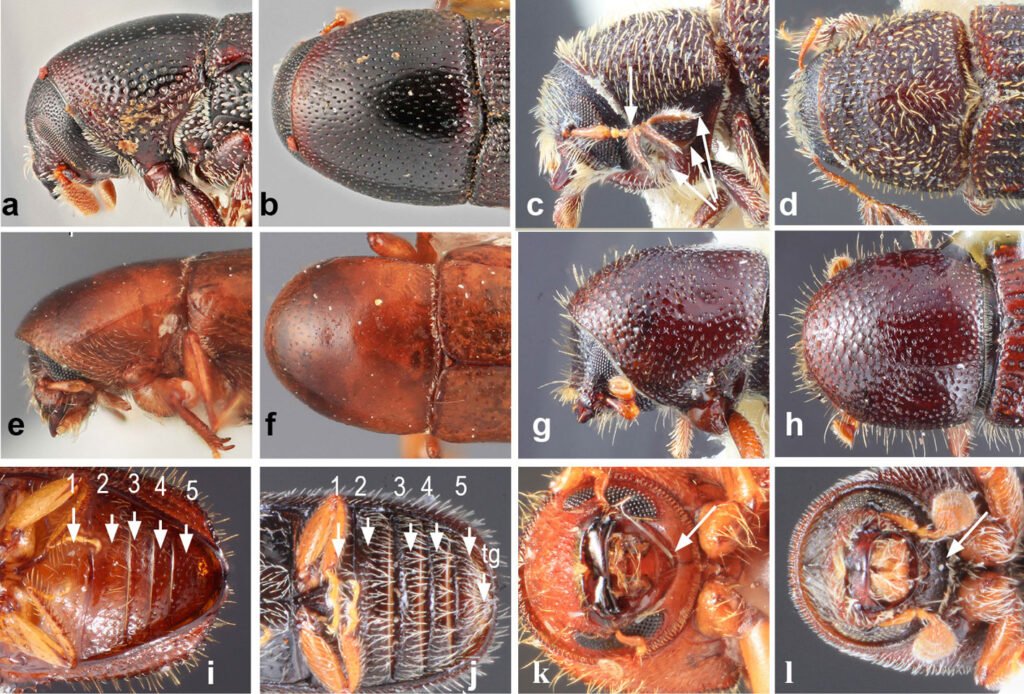
Figura 1. a, Vista lateral de cabeza y pronoto de Scolytopsis toba;b, vista dorsal de cabeza y pronoto de S. toba; c, vista lateral de cabeza y pronoto de Phloeotribus harringtoni; d, vista dorsal de cabeza y pronoto de P. harringtoni; e, vista lateral de cabeza y pronoto de Scolytodes tucumani; f, vista dorsal de cabeza y pronoto de S. tucumani; g, vista lateral de cabeza y pronoto de Orthotomicus laricis; h, vista dorsal de cabeza y pronoto de O. laricis; i, vista ventral del abdomen de Xyleborus volvulus; j, vista ventral del abdomen de Araptus sp.; k, vista ventral de partes bucales de Xylosandrus crassiusculus; l, vista ventral de partes bucales de Araptus pubescens.
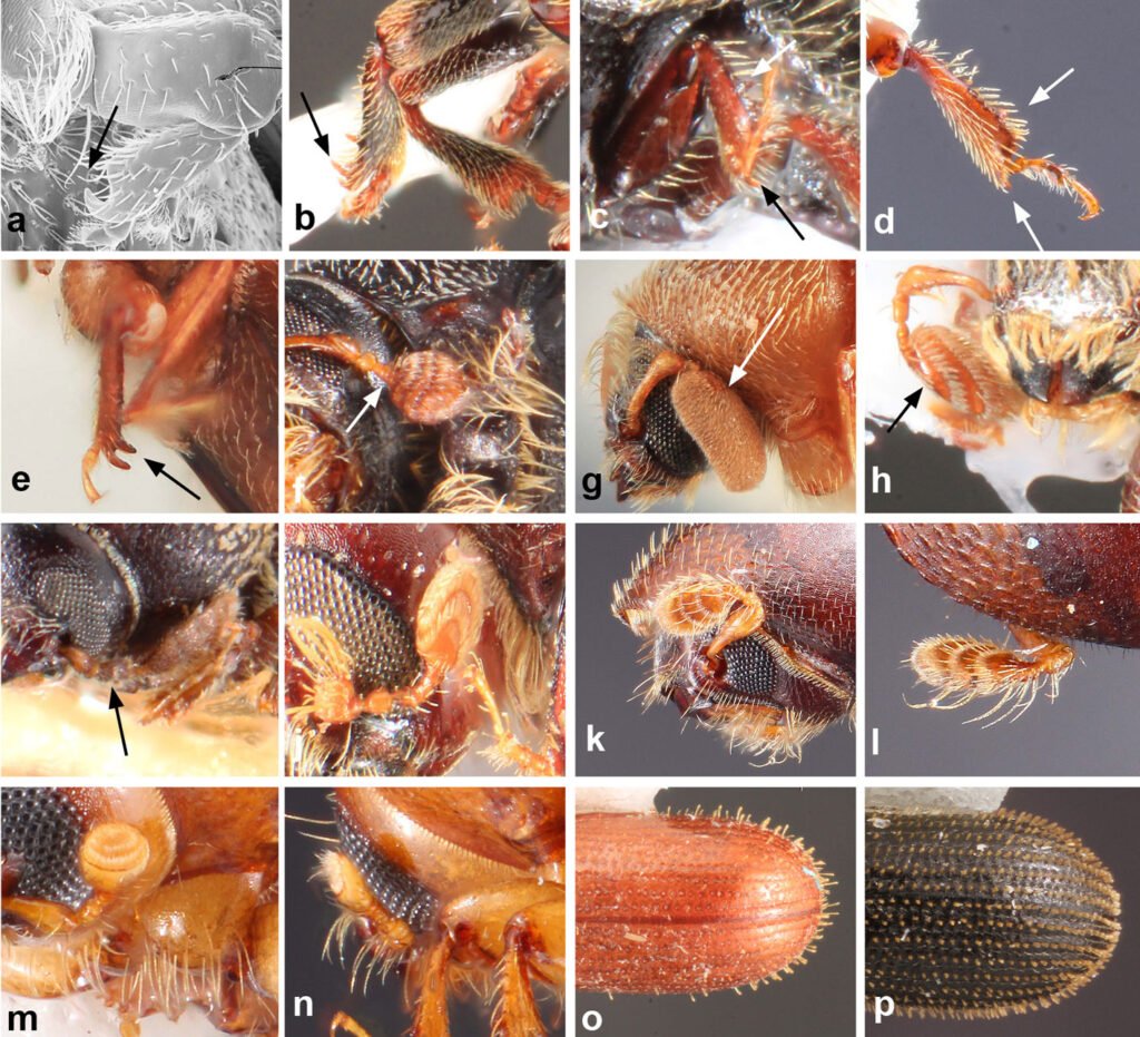
Figura 2. a, Protibia de Scolytopsis puncticollis; b, protibia de Pagiocerus frontalis; c, protibia de Coccotrypes carpophagus; d, protibia de Orthotomicus laricis; e, protibia de Scolytodes tucumani; f, antena de Xylechinus imperialis; g, antena de Chramesus argentiniae; h, antena de Pseudochramesus acuteclavatus; i, antena de Acorthylus bosqui; j, antena de Hylocurus giganteus; k, vista de cara anterior de la antena de Gnathotrichus sulcatus; l, vista de cara posterior de la antena de G. sulcatus; m, vista de cara anterior de la antena de Xyleborus volvulus; n, vista de cara posterior de la antena de X. volvulus; o, disco y declive elitral de Cryptocarenus seriatus; p: disco y declive elitral de Hypothenemus crudiae.
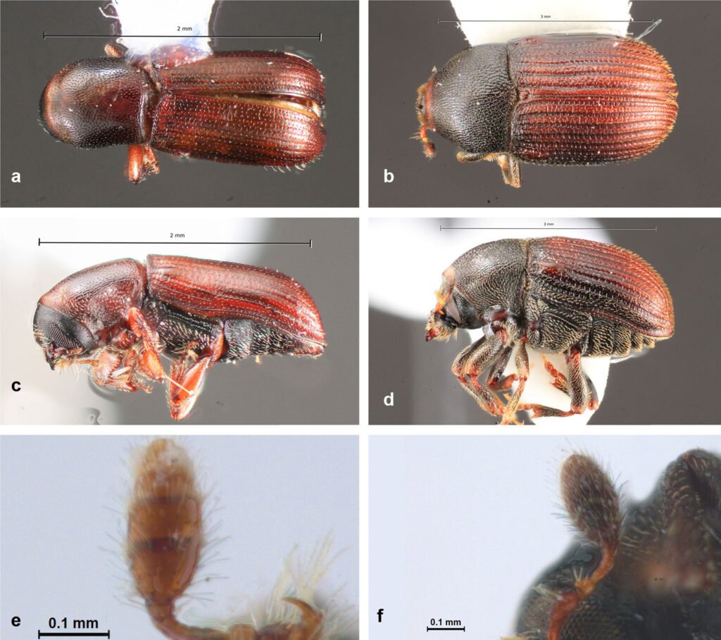
Figura 3. a: Vista dorsal de Cnesinus dividuus (tomada de Atkinson, 2025); b, vista dorsal de Pagiocerus frontalis (tomada de Atkinson, 2025); c, vista lateral de C. dividuus (tomada de Atkinson, 2025); d, vista lateral de P. frontalis (tomada de Atkinson, 2025); e, antena de C. dividuus;f, antena de P. frontalis.
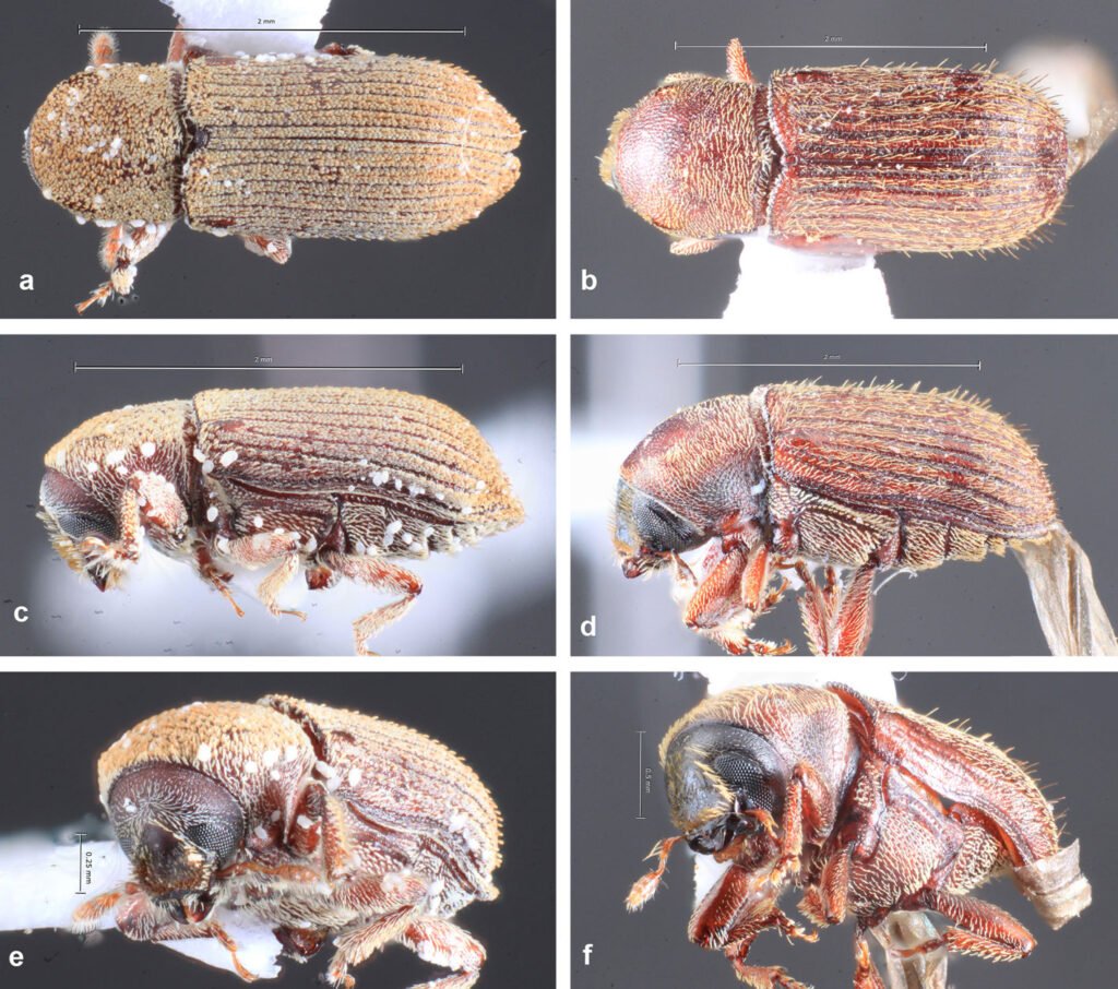
Figura 4. a, Vista dorsal de Cnesinus squamifer (tomada de Atkinson, 2025); b, vista dorsal de C. hispidus (tomada de Atkinson, 2025); c, vista lateral de C. squamifer (tomada de Atkinson, 2025); d, vista lateral de C. hispidus (tomada de Atkinson, 2025); e, vista frontal de C. squamifer (tomada de Atkinson, 2025); f, vista frontal de C. hispidus (tomada de Atkinson, 2025).
Subtribu Corthylina LeConte, 1876
Funículo antenal con 1-5 segmentos, maza grande y generalmente asimétrica; pieza intercoxal prosternal ausente, pubescencia comúnmente muy reducida, es insignificante muy confusa (no ordenada en filas); el declive elitral es convexo o truncado a profundamente excavado, generalmente con procesos similares a espinas. La mayoría de las especies perforan los tejidos del xilema del huésped e inoculan esporas de sus hongos simbióticos en las paredes del túnel, luego se alimentan principalmente de las esporas del hongo y el micelio (Wood, 2007).
Clave de las especies de la subtribu Corthylina
1. Funículo antenal de 2 segmentos; masa antenal truncada apicalmente, ovalada o redonda 2
1’. Funículo antenal de 1 segmento; masa antenal ovalada o redonda 3
2. Cuerpo castaño con 3 manchas más claras y rojizas en base del pronoto y 2 manchas alargadas longitudinales amarillentas en élitros, van desde la base hasta antes del declive elitral (fig. 5a, c); pronoto 1.5 veces más largo que ancho, borde anterior del pronoto armado con dientes; declive elitral amplio, moderadamente cóncavo, espina 1 en interestría 1 diminuta y puntiaguda, 2 en interestría 2, ligeramente más grandes que 1, espina 3 diminuta, espina 4 ligeramente más grandes que 2, puntiagudas (fig. 5e Monarthrum chapuisi Kirsch
2’. Cuerpo castaño rojizo muy oscuro y homogéneo (fig. 5b, d); pronoto 1.3 veces más largo que ancho, borde anterior del pronoto liso (sin dientes); declive elitral empinado, reticulado, estrecho y suavemente impreso, con espinas 2 y 3 diminutas (fig. 5f Monarthrum subimpressum Wood
3. Maza antenal 1.5 veces más larga que ancha, con sutura visible y cirro delgado (fig. 6e); frente fuertemente cóncava, mitad inferior amarillenta y esponjosa, sin setas (fig. 6g); margen anterior del pronoto débilmente aserrado; declive elitral muy empinado, redondeado y convexo, con setas erectas largas difusas (fig. 6c) Corthylus alineus Schedl
3’. Maza antenal 1.3 veces más larga que ancha, con 3 suturas visibles y cirro muy largo (fig. 6f); frente moderadamente cóncava, con áreas laterales a ambos lados de la frente, amarillas y esponjosas, con setas largas y erectas a ambos lados del área esponjosa (fig. 6h); borde apical de la frente con fila de setas plumosas orientadas hacia el centro de la frente; margen anterior del pronoto con espinas; declive elitral muy empinado (casi truncado) débilmente convexo, con cresta costal elevada no cerrada, con escasas setas largas y erectas (fig. 6d) Corthylus serrulatus Eggers
Monarthrum chapuisi Kirsch, 1866 (fig. 3a, c, e)
Distribución. Argentina: Tucumán; América del Sur: Bolivia, Colombia, Perú y Venezuela (Atkinson, 2025; Córdoba et al., 2023, 2025; Smith et al., 2017; Wood, 2007).
Monarthrum subimpressum Wood, 2007 (fig. 5b, d, f)
Distribución. Argentina: Salta, Tucumán (Atkinson, 2025; Córdoba et al., 2023, 2025; Wood, 2007).
Corthylus alineus Schedl, 1966 (fig. 6a, c, e, g)
Distribución. Argentina: Salta y Tucumán; América del Sur: Colombia, Ecuador y Perú (Atkinson, 2025; Córdoba y Atkinson, 2018; Córdoba et al., 2023, 2025; Smith et al., 2017; Wood, 2007).
Corthylus serrulatus Eggers, 1934 (fig. 6b, d, f, h)
Distribución. Argentina: Jujuy, Salta y Tucumán; América del Sur: Bolivia, Brasil y Perú (Atkinson, 2025; Córdoba et al., 2018, 2021, 2023, 2025; Smith et al., 2017; Wood, 2007).
Subtribu Pityophthorina Eichhoff, 1878
Se caracteriza por presentar el funículo antenal mayormente de 5 segmentos, maza antenal más pequeña y simétrica; pieza intercoxal prosternal agudamente puntiaguda; pubescencia abundante, generalmente en filas en los élitros; declive elitral comúnmente convexo a bisulcado, armadura ausente. Se alimentan directamente del tejido de la planta huésped y son floeófagas, mielófagas o espermófagas. No hay especies verdaderamente xilófagas (Wood, 2007).
Clave de las especies de la subtribu Pityophthorina
1. Revestimiento del cuerpo formado por escamas (fig. 7a, b); flagelo antenal con 2 segmentos; maza antenal alargada y subrectangular (fig. 7c); pronoto con 8 filas transversales de espinas romas; ramillete de setas largas en cara interna de protibias, que van desde la base hasta el ápice de las mismas (fig. 7e); menos de 2 mm de longitud del cuerpo Acorthylus bosqui (Schedl)
1’. Revestimiento del cuerpo formado por setas; flagelo antenal con 4 segmentos; maza antenal redondeada y aplanada (fig. 7d); pronoto con espinas romas o sin espinas; tibias anteriores con pubescencia abundante (fig. 7f); más de 2 mm de longitud del cuerpo 2
2. Pronoto con rugosidades pronunciadas en la parte anterior; pronoto en vista lateral, convexo hasta el disco, luego con una elevación pronunciada en medio, más bajo y recto hasta la base; maza antenal con 2 suturas parcial o totalmente septadas 3
2’. Pronoto sin rugosidades pronunciadas en la parte anterior; pronoto en vista lateral con curvatura uniforme desde el ápice hasta la base, sin elevación pronunciada; maza antenal con 1 sutura total o parcialmente septada 5
3. Declive elitral con sulcos, interestría 1 moderadamente elevada, armada por 10 o más tubérculos; pubescencia de los élitros confinada al declive (fig. 9e) Pityophthorus tucumanensis Wood
3’. Declive elitral completamente convexo, sin sulcos, interestría 1 sin tubérculos 4
4. Longitud del cuerpo 1.4 a 1.8 mm; frente con fuerte impresión transversal y con pequeño tubérculo medio a nivel de los ojos (fig. 8e); color del cuerpo castaño oscuro (fig. 8a, c) Cryptocarenus heveae (Hagedorn)
4’. Longitud del cuerpo 1.4 a 1.5 mm; frente cóncava (fig. 8f); coloración del cuerpo castaño rojizo o claro (fig. 8b, d) Cryptocarenus seriatus Eggers
5. Pronoto de lados paralelos; élitros 2 veces más largos que el pronoto (fig. 9b, d) Araptus araujiae (Brèthes)
5’. Pronoto de lados convexos; élitros entre 1.6 y 1.7 más largos que el pronoto 6
6. Frente con quilla media aguda, más fuertemente elevada en mitad media superior (fig. 10g); maza antenal redondeada; pubescencia del cuerpo abundante (fig. 10a,d) Araptus pubescens (Schedl)
6’. Frente sin quilla; maza antenal ovalada; pubescencia no muy abundante 7
7. Frente muy débilmente convexa, con pubescencia corta y escasa (fig. 10h); declive elitral convexo y bisulcado (fig. 10j) Araptus frenatus (Schedl)
7’. Frente claramente convexa, con pubescencia larga abundante y erecta; con tubérculo en el ápice de la frente, poco marcado que se afina hasta la base (fig. 10i); declive elitral convexo con surco poco profundo en las interestrías 1 y 2 (fig. 10k) Araptus volastos (Schedl)
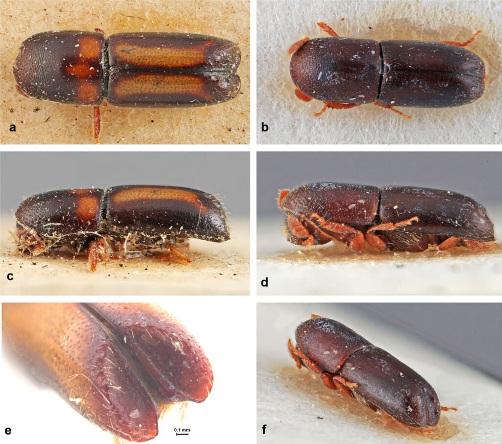
Figura 5. a, Vista dorsal de Monarthrum chapuisi (tomada de Atkinson, 2025); b, vista dorsal de M. subimpresum (tomada de Atkinson, 2025); c, vista lateral de M. chapuisi (tomada de Atkinson, 2025); d, vista lateral de M. subimpresum (tomada de Atkinson, 2025); e, vista posterior de M. chapuisi; f, vista posterior de M. subimpresum (tomada de Atkinson, 2025).
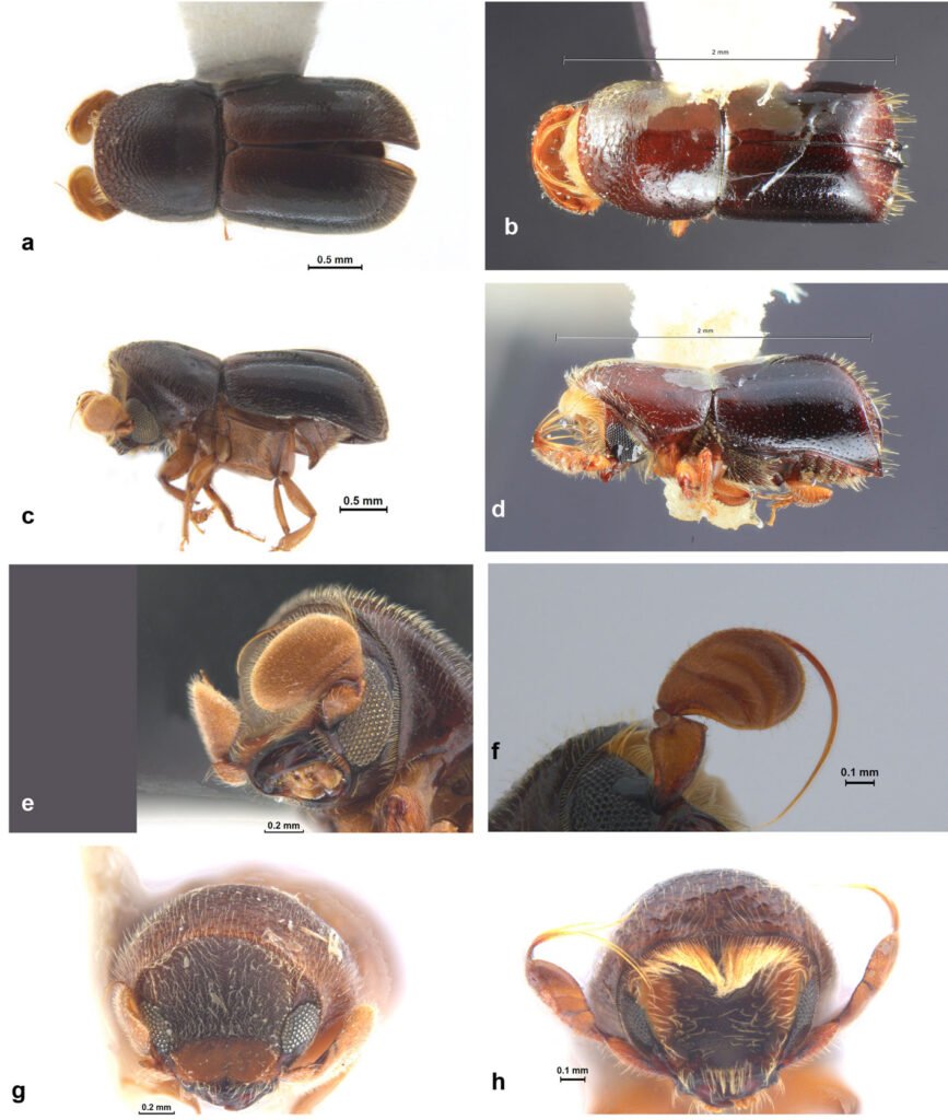
Figura 6. a, Vista dorsal de Corthylus alineus;b, vista dorsal de C. serrulatus (tomada de Atkinson, 2025); c, vista lateral de C. alineus; d, vista lateral de C. serrulatus (tomada de Atkinson, 2025); e, antena de C. alineus; f, antena de C. serrulatus; g, vista frontal de C. alineus; h, vista frontal de C. serrulatus.
Acorthylus bosqui (Schedl, 1938) (fig. 7a, b, c, e)
Distribución. Argentina: Jujuy y Tucumán; América del Sur: Bolivia (Atkinson, 2025; Córdoba et al., 2023, 2025; Wood, 2007).
Cryptocarenus heveae (Hagedorn, 1912) (fig. 7d, f, 8a, c, e)
Distribución. Argentina: Buenos Aires, Misiones, Santiago del Estero y Tucumán; América del Sur: Brasil, Colombia Perú, Trinidad y Tobago y Venezuela (Atkinson, 2025; Córdoba et al., 2021, 2023, 2025; Iturre y Darchuck, 1996; Smith et al., 2017; Wood, 2007).
Cryptocarenus seriatus Eggers, 1933 (fig. 8b, d, f)
Distribución. Argentina: Tucumán; América del Sur: Bolivia, Brasil, Colombia, Guyana Francesa, Paraguay, Perú y Venezuela (Atkinson 2025; Córdoba et al., 2023, 2025; Smith et al., 2017; Wood, 2007).
Pityophthorus tucumanensis Wood, 2007 (fig. 9a, c, e)
Distribución. Argentina: Tucumán (Atkinson, 2025; Córdoba et al., 2023, 2025; Wood, 2007).
Araptus araujiae (Brèthes, 1921) (fig. 9b, d)
Distribución. Argentina: Buenos Aires y Tucumán (Atkinson, 2025; Bachmann y Lanteri, 2013; Córdoba et al., 2023, 2025; Wood y Bright, 1992).
Araptus pubescens (Schedl, 1950) (fig. 10a, d, g)
Distribución. Argentina: Córdoba y Tucumán (Atkinson, 2025; Córdoba et al., 2025; Wood, 2007).
Araptus frenatus (Schedl, 1939) (fig. 10b, e, h, j)
Distribución. Argentina: Córdoba y Tucumán (Atkinson, 2025; Córdoba et al., 2025; Wood, 2007).
Araptus volastos (Schedl, 1938) (fig. 10c, f, i, k)
Distribución. Argentina: Jujuy, Salta y Tucumán; América del Sur: Bolivia (Atkinson, 2025; Córdoba et al., 2025; Wood, 2007).
Tribu Dryocoetini Lindemann, 1877
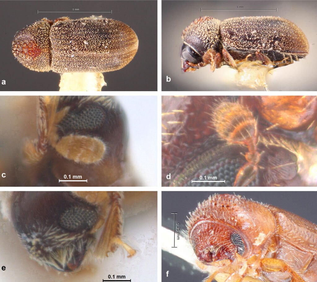
Figura 7. a, Vista dorsal de Acorthylus bosqui (tomada de Atkinson, 2025); b, vista lateral de A. bosqui (tomada de Atkinson, 2025); c, antena de A. bosqui; d, antena de Cryptocarenus heveae; e, tibia de A. bosqui; f, tibia de C. heveae (tomada de Atkinson, 2025).
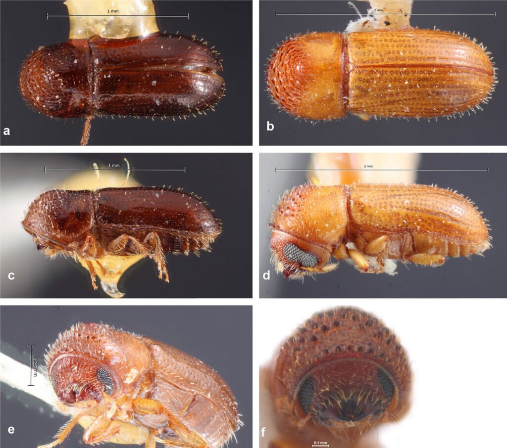
Figura 8. a, Vista dorsal de Cryptocarenus heveae (tomada de Atkinson, 2025); b, vista dorsal de C. seriatus (tomada de Atkinson, 2025); c, vista lateral de C. heveae (tomada de Atkinson, 2025); d, vista lateral de C. seriatus (tomada de Atkinson, 2025); e, vista frontal de C. heveae (tomada de Atkinson, 2025); f, vista frontal de C. seriatus
Presentan dimorfismo sexual en la frente. En los machos es convexa a variadamente impresa y en las hembras es convexa a aplanada o con elevaciones; el ojo está emarginado o dividido; el escapo antenal es alargado, el funículo está compuesto de 4 a 6 segmentos, la maza antenal puede estar oblicuamente truncada o conspicuamente aplanada, en este último caso las suturas son procurvadas u obsoletas; el pronoto puede estar o no armado con asperezas; las procoxas pueden ser contiguas o estar muy poco separadas; margen lateral de las protibias con 3 o más dentículos alveolares; el declive elitral puede ser convexo, sulcado, aplanado y, a veces, con pequeños gránulos; la pubescencia está compuesta por setas; la mayoría de las especies son polígamas y algunas son haploides; hay especies espermatófagas, mielófagas y floeófagas. De los 17 géneros que se conocen en el mundo, solo 4 se encuentran en América del Sur, pero 2 de ellos son introducidos (Wood, 2007). Las especies del género Coccotrypes presentes en la región son barrenadores de semillas de palmeras.
Clave de las especies de la tribu Dryocoetini
1. Tamaño del cuerpo entre 1.8 a 2.3 mm; pubescencia moderadamente abundante (fig. 11a, c); pronoto de lados marcadamente convexos que se angosta de manera abrupta hacia el ápice, con asperezas pequeñas y abundantes (fig. 11a) Coccotrypes dactyliperda (Fabricius)
1’. Tamaño del cuerpo entre 1.5 y 1.9 mm; pubescencia muy abundante (fig. 11b, d); pronoto redondeado, angostado en el ápice, con asperezas gruesas y marcadas (fig. 11b) Coccotrypes carpophagus (Hornung)
Coccotrypes dactyliperda (Fabricius, 1801)* (fig. 11a, c)
Distribución. S/D, Tucumán (Atkinson, 2025; Córdoba et al., 2023, 2025; Wood y Bright, 1992).
Coccotrypes carpophagus (Hornung, 1842)* (fig. 11b, d)
Distribución. Tucumán (Atkinson, 2025; Córdoba et al., 2023, 2025).
Tribu Hexacolini Eichhoff, 1878
Sus miembros presentan dimorfismo sexual: los machos pueden presentar una impresión en la frente, a veces oscura; los machos son convexos y las hembras son esculpidas y ornamentadas de forma variada; los ojos son en general alargados, con su margen anterior entero o sinuoso; el escapo antenal es alargado; el funículo lleva 5 o 6 segmentos (con 7 segmentos en Gymnochilus); la maza antenal puede o no llevar suturas; la zona apical del pronoto puede estar ornamentada o no; las procoxas están ampliamente separadas; las protibias llevan, en el margen lateral, 1 o más dentículos alveolares generalmente incrustados en la cutícula (Wood, 2007).
Clave de las especies de la tribu Hexacolini
1. Color castaño amarillento, con franja más oscura en mitad apical del pronoto (fig. 12a, c); frente con callo transversal por debajo del nivel superior de ojos (fig. 12e); pronoto con superficie reticulada; élitros de lados convexos (fig. 12a); declive elitral ampliamente convexo (fig.12c) Scolytodes sparsepilosus Wood
1’. Color castaño amarillento, con mitad apical más oscura (fig. 12b, d); frente con callo medio estrecho que se extiende dorsalmente desde elevación epistomal hasta ligeramente por encima del nivel de inserción de antena (fig. 12f); pronoto liso y brillante; élitros de lados paralelos (fig. 12b); declive estrechamente convexo (fig. 12d) Scolytodes tucumani Wood
Scolytodes sparsepilosus Wood, 2007 (fig. 12a, c, e)
Distribución. Argentina: Tucumán (Atkinson, 2025; Córdoba et al., 2023, 2025; Wood, 2007).
Scolytodes tucumani Wood, 2007 (fig. 12b, d, f)
Distribución. Argentina: Tucumán; América del Sur: Ecuador (Atkinson, 2025; Córdoba et al., 2023, 2025; Jordal y Smith, 2020; Wood, 2007).
Tribu Hylurgini Gistel, 1848
Presentan dimorfismo sexual en la frente, siendo convexa en las hembras e impresa en los machos; los ojos son enteros y ovalados; las antenas presentan un escapo alargado, el funículo con 5 a 7 segmentos y la maza antenal es simétrica, aplanada y generalmente con 3 o 4 suturas; el pronoto es generalmente liso; las procoxas son contiguas o están muy poco separadas; las tibias están armadas por dientes en los márgenes laterales y apicales; todas las especies de esta tribu son monógamas y fleófagas (Wood, 2007).
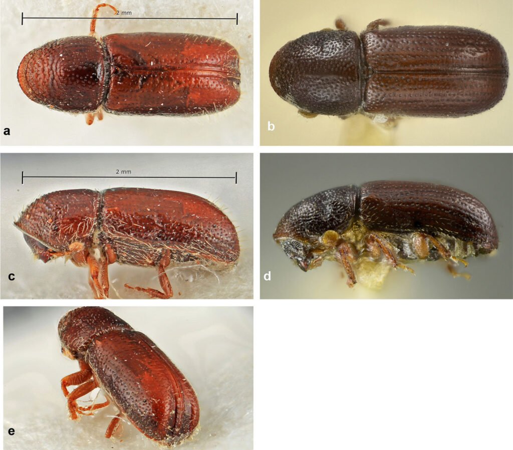
Figura 9. a, Vista dorsal de Pityophthorus tucumanensis (tomada de Atkinson, 2025); b, vista dorsal de Araptus araujiae; c, vista lateral de P. tucumanensis (tomada de Atkinson, 2025); d, vista lateral de A. araujiae; e, vista posterior de P. tucumanensis (tomada de Atkinson, 2025).
Clave de las especies de la tribu Hylurgini
Longitud 2.1-2.6 mm; color castaño oscuro, con pubescencia formada por setas y escamas con patrón de coloración mezclada (fig. 13a, b); frente convexa, reticulada y rugosa por encima de los ojos y lisa y brillante por debajo de ellos (fig. 13c); pronoto 0.85 veces más largo que ancho, base más ancha que el ápice, lados convexos, con superficie reticulada (fig. 13a); interestrías de élitros armadas por tubérculos; en macho las interestrías 3 y base de la 1 elevadas y armadas por dentículos en declive elitral Xylechinus imperialis (Schedl)
Xylechinus imperialis (Schedl, 1958) (fig. 13a-c)
Distribución. Argentina: Buenos Aires, Jujuy, Salta, Santa Fe y Tucumán (Atkinson, 2025; Córdoba et al., 2023, 2025; Wood, 2007).
Tribu Ipini Bedel, 1888
Se distinguen por presentar dimorfismo sexual en la frente, siendo convexa en los machos y de forma variada en las hembras; la antena presenta un escapo afinado y alargado, el funículo antenal está formado por 5 segmentos y la maza puede ser oblicuamente truncada o aplanada, con suturas desplazadas hacia el ápice de la cara posterior; mitad anterior del ápice del pronoto es declivado y áspero; las procoxas son contiguas; protibias presentan 3 o 4 dientes; el declive elitral es sulcado o profundamente excavado, puede estar armado con espinas o tubérculos; el cuerpo presenta una pubescencia similar a setas. Todas las especies de esta tribu son floeófagas y monógamas o polígamas (Wood, 2007).
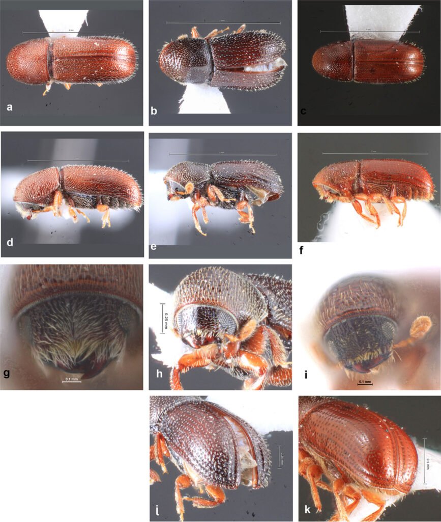
Figura 10. a, Vista dorsal de Araptus pubescens (tomada de Atkinson, 2025); b, vista dorsal de A. frenatus (tomada de Atkinson, 2025); c, vista dorsal de A. volastos (tomada de Atkinson, 2025); d, vista lateral de A. pubescens (tomada de Atkinson, 2025); e, vista lateral de A. frenatus (tomada de Atkinson, 2025); f: vista lateral de A. volastos (tomada de Atkinson, 2025); g: vista frontal de A.pubescens; h, vista frontal de A. frenatus (tomada de Atkinson, 2025); i, vista frontal de A. volastos; j, vista posterior de A. frenatus (tomada de Atkinson, 2025); k, vista posterior de A. volastos (tomada de Atkinson, 2025).

Figura 11. a, Vista dorsal de Coccotrypes dactyliperda (tomada de Atkinson, 2025); b, vista dorsal de C. carpophagus (tomada de Atkinson, 2025); c, vista lateral de C. dactyliperda (tomada de Atkinson, 2025); d, vista lateral de C. carpophagus (tomada de Atkinson, 2025).
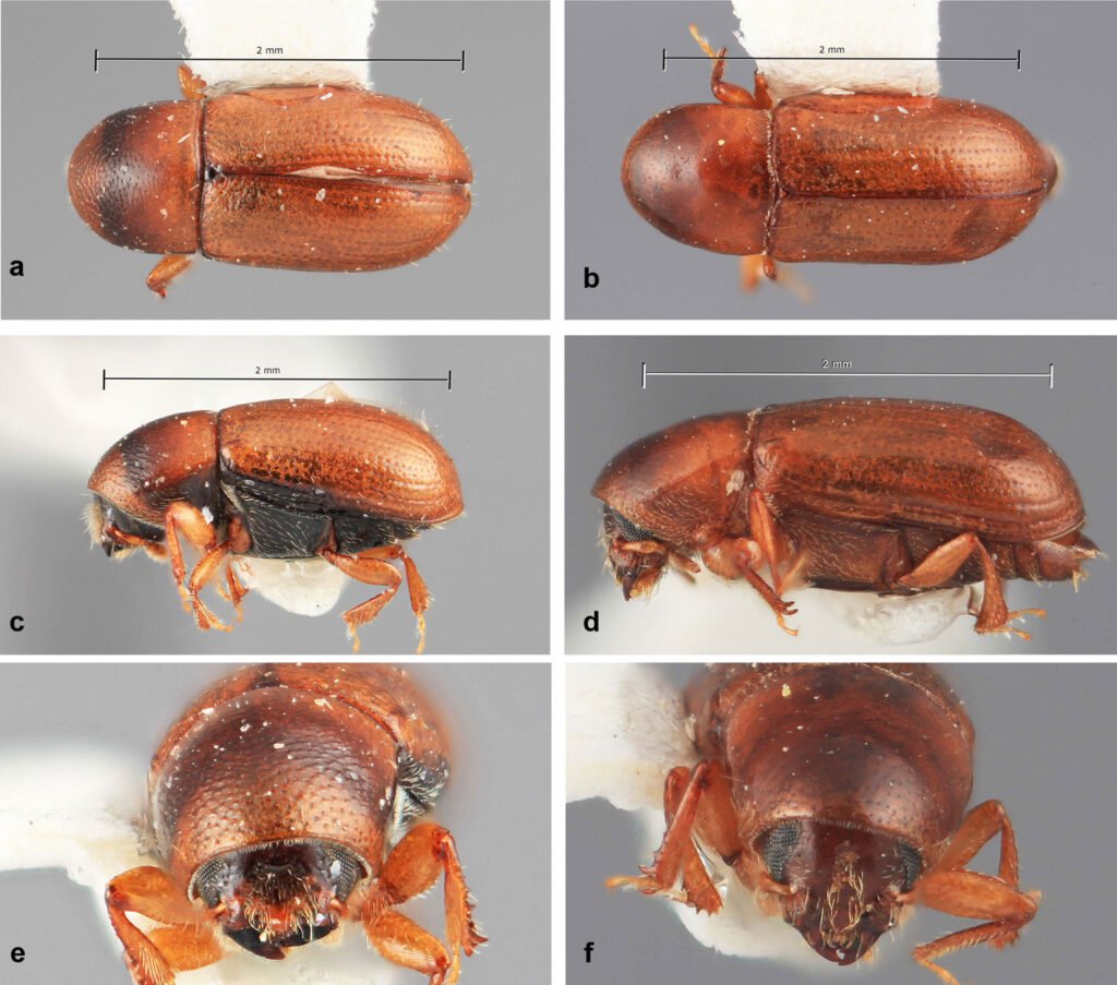
Figura 12. a, Vista dorsal de Scolytodes sparsepilosus (tomada de Atkinson, 2025); b, vista dorsal de S. tucumani (tomada de Atkinson, 2025); c, vista lateral de S. sparsepilosus (tomada de Atkinson, 2025); d, vista lateral de S. tucumani (tomada de Atkinson, 2025); e, vista frontal de S. sparsepilosus (tomada de Atkinson, 2025); f, vista frontal de S. tucumani (tomada de Atkinson, 2025).
Clave de las especies de la tribu Ipini
(Macho) Longitud: 3.0-3.7 mm; 2.7 veces más largo que ancho (fig. 14a, b); frente levemente convexa con abundante pubescencia larga, fina y erecta; pronoto 1,07 veces más largo que ancho, mitad anterior moderadamente declinada y mitad basal levemente cóncava, con pubescencia escasa en el centro y con setas largas y erectas en los bordes y ápice (fig. 14b); declive elitral cóncavo, con 3 espinas en bordes externos, 1 espina en interestría 1 y otra en la interestría 2 (fig. 14c) Orthotomicus laricis (Fabricius)
Orthotomicus laricis (Fabricius, 1792)* (fig. 14a, b, c)
Distribución. Argentina: Neuquén y Tucumán; América del Sur: Chile (Atkinson, 2025; Córdoba et al., 2021, 2023, 2025; Kirkendall, 2018; Wood, 2007).
Tribu Micracidini LeConte, 1876
Se distinguen por presentar dimorfismo sexual en la frente, siendo en la hembra generalmente cóncava y en el macho, raramente cóncava; los ojos pueden ser ovalados, alargados, enteros o sinuados; antenas con el escapo corto o alargado, aplanado o expandido, con setas, el funículo presenta 6 segmentos, la maza antenal puede o no tener suturas; el pronoto presenta asperezas en la zona anterior, los lados son redondeados; las procoxas están ligeramente separadas; generalmente presentan setas subplumosas en alguna parte del cuerpo; pueden tener hábitos xilófagos, floeófagos o mielófagos; todos son bígamos excepto el género Micraciella que es monógamo (Wood, 2007).
Clave de las especies de la tribu Micracidini
(Macho) Longitud 3.2 a 3.5 mm; 2.8 veces más largo que ancho; frente convexa con carena transversal (fig. 15c); antena con escapo ligeramente aplanado con mechón de pelos (fig. 15c), sutura procurvada; mitad apical del pronoto con tubérculos que van disminuyendo hacia la mitad, margen apical con 6 dientes; declive elitral convexo con nódulos en las interestrías de la base, interestría 9 con quilla, pubescencia escasa, aumenta en el declive elitral, élitros terminados en punta aguda (fig. 15d) Hylocurus giganteus (Schedl)
Hylocurus giganteus (Schedl, 1950) (fig. 15a-d)
Distribución. Argentina: Salta y Tucumán; América del Sur: Brasil (Atkinson, 2025; Córdoba et al., 2023, 2025; Wood, 2007).
Tribu Phloeosinini Nüsslin, 1912
Presentan dimorfismo sexual en la frente, machos con diferentes impresiones y hembras con frente aplanada o convexa; ojos pueden estar emarginados; antenas llevan un funículo con 5-7 segmentos, maza antenal aplanada, pueden ser asimétricas en diferentes medidas, pueden llevar suturas o no; pronoto no tiene asperezas, excepto en Dendrosinus, que presenta asperezas débiles; tercer segmento tarsal comprimido o bilobulado; escutelo puede o no ser visible; pueden ser polígamos o bígamos; pueden ser floeófagos o xilófagos (Wood, 2007).
Clave para las especies de la tribu Phloeosinini
1. Maza antenal fuertememente aplanada, en forma de riñón, la unión con el funículo es en su parte lateral, sin suturas ni fila de setas; escutelo presente pero diminuto; pronoto liso o reticulado 2
1’. Maza antenal con suturas fuertemente procurvadas y claramente marcadas por fila de setas, unión con el funículo excéntrica; escutelo visible; pronoto liso o armado con pequeños gránulos 4
2. Frente del macho con márgenes laterales fuertemente elevados y con cuentas 3
2’. Frente del macho con márgenes laterales agudamente elevados con cresta irregular pero sin cuentas (fig. 16g) Chramesus phloeotriboides Schedl
3. Margen lateral de la frente del macho fuertemente elevado y con cuentas solo en el tercio inferior (fig. 16h); maza antenal 2.6 veces más larga que ancha; pronoto con superficie lisa y brillante, zona basal con algunos tubérculos pequeños y aislados Chramesus argentinae Wood
3’. Margen lateral de la frente del macho agudamente elevado y marcado con 9 cuentas (fig. 16i); maza antenal 2.3 veces más larga que ancha; pronoto con zona basal profundamente punteada Chramesus globosus Hagedorn
4. Frente ampliamente convexa; estrías de los élitros claramente impresas o no impresas con punciones regulares 5
4’. Frente ancha y ligeramente cóncava (fig. 17g); estrías de los élitros impresas con punciones bastantes grandes; interestría 7 elevada en los machos Pseudochramesus costulatus Blackman
5. Interestrías con escamas de fondo castañas oscuras y pálidas, formando un patrón, setas pálidas uniseriadas en interestrías (fig. 17b, e); frente con elevación a nivel de inserción de antenas (fig. 17h) Pseudochramesus acuteclavatus (Hagedorn)
5’. Interestrías con escamas de fondo castañas, a lo largo de la sutura, pálidas (fig. 17c, f); frente sin elevación a nivel de la inserción de las antenas (fig. 17i) Pseudochramesus harringtoni Blackmann
Chramesus phloeotriboides Schedl, 1958 (fig. 16a, d, g)
Distribución. Argentina: Córdoba y Tucumán (Atkinson, 2025; Córdoba et al., 2023, 2025; Wood, 2007).
Chramesus argentinae Wood, 2007 (fig. 16b, e, h)
Distribución. Argentina: Tucumán (Atkinson, 2025; Córdoba et al., 2023, 2025; Wood, 2007).
Chramesus globosus Hagedorn, 1909 (fig. 16c, f, i)
Distribución. Argentina: Buenos Aires, La Rioja, Misiones, Santa Fe y Tucumán; América del Sur: Brasil y Uruguay (Atkinson, 2025; Bachmann y Lanteri, 2013; Córdoba et al., 2023, 2025; Wood, 2007).
Pseudochramesus costulatus Blackman, 1939 (fig. 17a, d, g)
Distribución. Argentina: Jujuy y Tucumán; América del Sur: Bolivia (Atkinson, 2025; Córdoba et al., 2023, 2025; Wood, 2007).
Pseudochramesus acuteclavatus (Hagedorn, 1909) (fig. 17b, e, h)
Distribución. Argentina: Buenos Aires, Salta y Tucumán; América del Sur: Bolivia, Brasil y Paraguay (Atkinson, 2025; Bachmann y Lanteri, 2013; Córdoba et al., 2023, 2025; Wood, 2007).
Pseudochramesus harringtoni Blackmann, 1939 (fig. 17c, f, i)
Distribución. Argentina: Salta y Tucumán; América del Sur: Bolivia y Brasil (Atkinson, 2025; Córdoba et al., 2023, 2025; Wood, 2007).
Tribu Phloeotribini Chapuis, 1869
Presentan dimorfismo sexual en la frente, siendo con impresiones variadas en los machos y planas o convexas en las hembras; los ojos son enteros; antenas con funículo de 5 segmentos, la maza antenal puede ser muy delgada o fuertemente asimétrica, está dividida en 3 segmentos móviles, usualmente sublamelados; las procoxas son contiguas; el pronoto puede llevar o no asperezas, los márgenes laterales son redondeados; son especies monógamas y floeófagas (Wood, 2007).
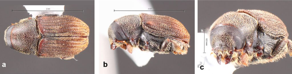
Figura 13. a, Vista dorsal de Xylechinus imperialis (tomada de Atkinson, 2025); b, vista lateral de X. imperialis (tomada de Atkinson, 2025); c, vista frontal de X. imperialis (tomada de Atkinson, 2025).
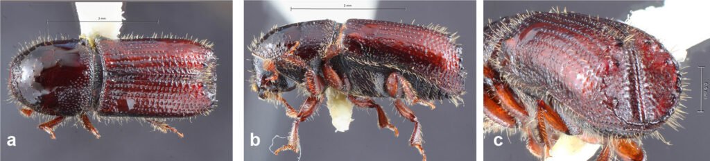
Figura 14. a, Vista dorsal de Orthotomicus laricis (tomada de Atkinson, 2025); b, vista lateral de O. laricis (tomada de Atkinson, 2025); c, vista frontal de O. laricis (tomada de Atkinson, 2025).
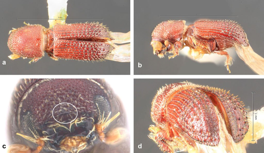
Figura 15. a, Vista dorsal de Hylocurus giganteus (tomada de Atkinson, 2025); b, vista lateral de H. giganteus (tomada de Atkinson, 2025); c, vista frontal de H. giganteus; d, vista posterior de H. giganteus (tomada de Atkinson, 2025).
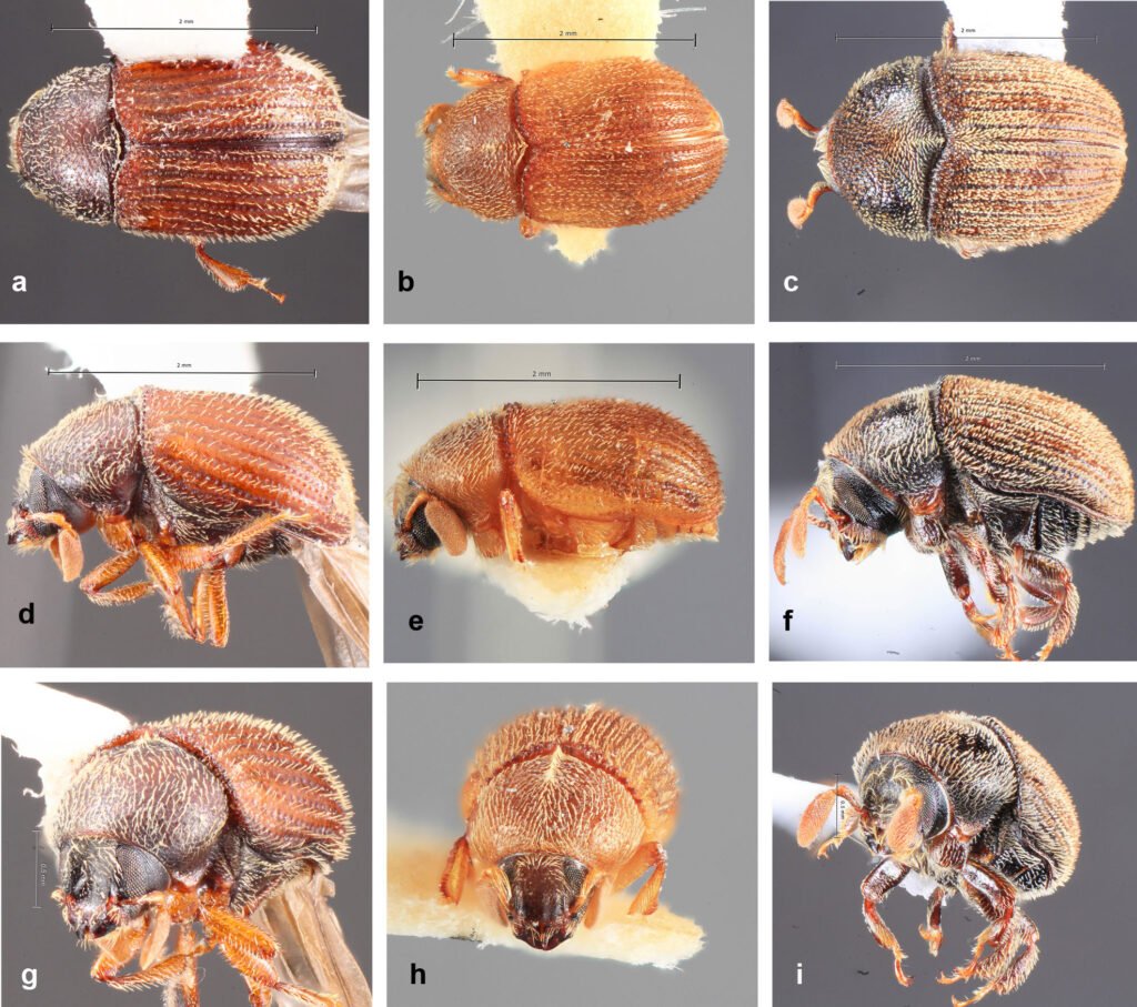
Figura 16. a, Vista dorsal de Chramesus phloeotriboides (tomada de Atkinson, 2025); b, vista dorsal de C. argentinae (tomada de Atkinson, 2025); c, vista dorsal de C. globosus (tomada de Atkinson, 2025); d, vista lateral de C. phloeotriboides (tomada de Atkinson, 2025); e, vista lateral de C. argentinae (tomada de Atkinson, 2025); f, vista lateral de C. globosus (tomada de Atkinson, 2025); g, vista frontal de C. phloeotriboides (tomada de Atkinson, 2025); h, vista frontal de C. argentinae (tomada de Atkinson, 2025); i, vista frontal de C. globosus (tomada de Atkinson, 2025).
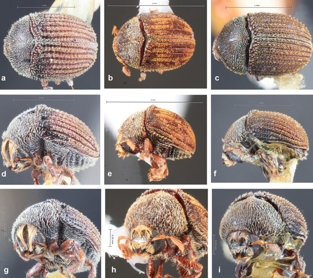
Figura 17. a, Vista dorsal de Pseudochramesus costulatus (tomada de Atkinson, 2025); b, vista dorsal de P. acuteclavatus (tomada de Atkinson, 2025); c, vista dorsal de P. harringtoni (tomada de Atkinson, 2025); d, vista lateral de P. costulatus (tomada de Atkinson, 2025); e, vista lateral de P. acuteclavatus (tomada de Atkinson, 2025); f, vista lateral de P. harringtoni (tomada de Atkinson, 2025); g, vista frontal de P. costulatus (tomada de Atkinson, 2025); h, vista frontal de P. acuteclavatus (tomada de Atkinson, 2025); i, vista frontal de P. harringtoni (tomada de Atkinson, 2025).
Clave para las especies de la tribu Phloeotribini
1. Frente con área cóncava; pronoto con crenulaciones en mitad apical y puntos grandes; élitros con interestrías iguales o más angostas que estrías; declive elitral con espinas 2
1’. Frente con área cóncava y carena epitosmal muy elevada en macho (fig. 18g); pronoto con asperezas en mitad apical y puntos medianos; élitros con interestrías 3 veces más anchas que estrías; declive elitral con tubérculos pequeños (fig. 18j) Phloeotribus subovatus Blandford
2. Escapo antenal con mechón grande de setas largas (fig. 18h); interestrías de igual ancho que estrías; declive elitral con tubérculos espiniformes en interestrías 2-9 (fig. 18k) Phloeotribus asperulus Eggers
2’. Escapo antenal con escasas setas (fig. 18i); interestrías más angostas que las estrías; declive elitral con espinas en las interestrías 1 a la 9 (fig. 18l) Phloeotribus harringtoni Blackman
Phloeotribus subovatus Blandford, 1897 (fig. 18a, d, g, j)
Distribución. Argentina: Jujuy, Salta y Tucumán; América del Sur: Perú y Venezuela (Atkinson, 2025; Córdoba et al., 2025; Wood, 2007).
Phloeotribus asperulus Eggers, 1943 (fig. 18b, e, h, k)
Distribución. Argentina: Tucumán; América del Sur:
Bolivia y Brasil (Atkinson, 2025; Córdoba et al., 2025; Wood y Bright, 1992).
Phloeotribus harringtoni Blackman, 1943 (fig. 18c, f, i, l)
Distribución. Argentina: Salta y Tucumán (Atkinson, 2025; Córdoba et al., 2023, 2025; Wood, 2007).
Tribu Scolytini Latreille, 1804
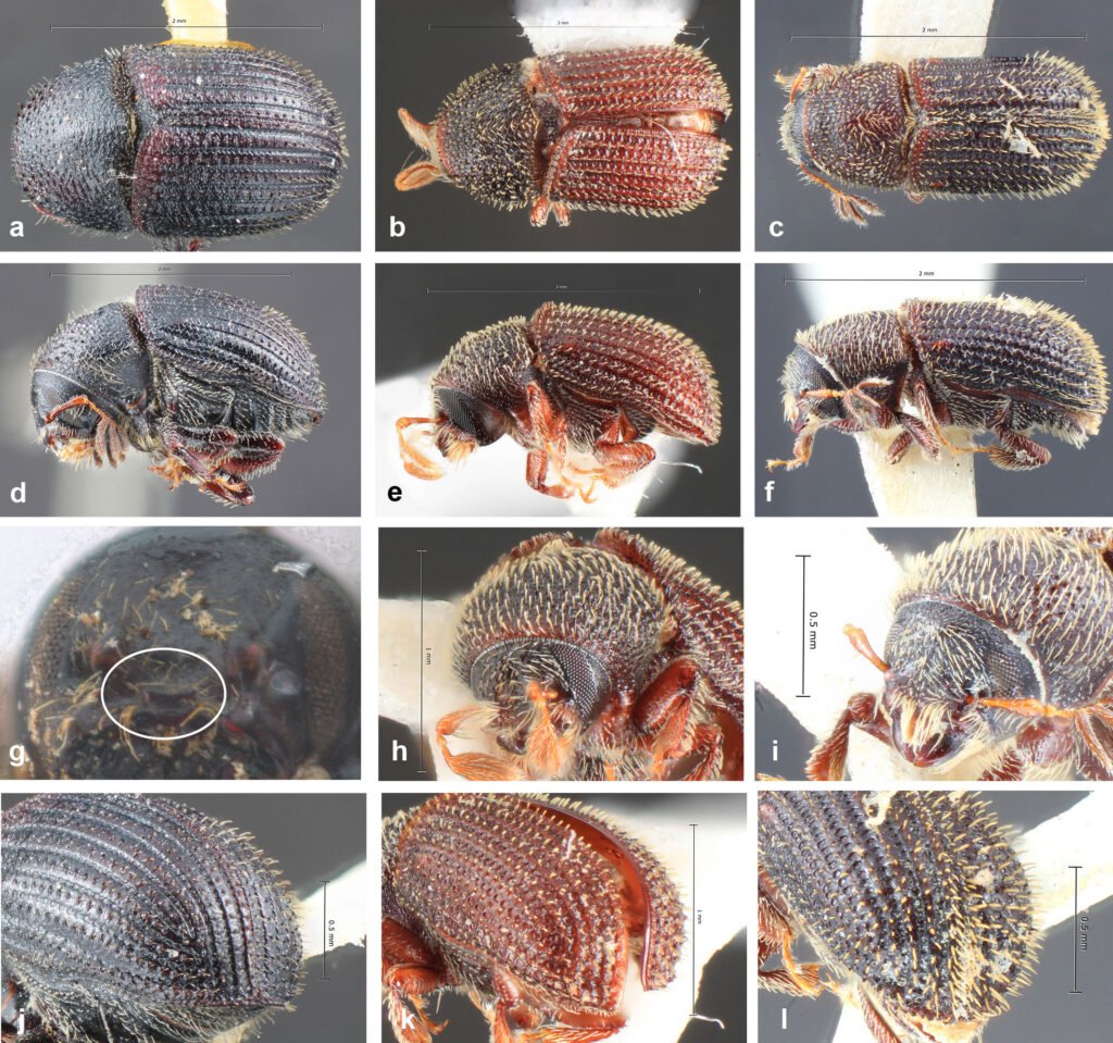
Figura 18. a, Vista dorsal de Phloeotribus subovatus (tomada de Atkinson, 2025); b, vista dorsal de P. asperulus (tomada de Atkinson, 2025); c, vista dorsal de P. harringtoni (tomada de Atkinson, 2025); d, vista lateral de P. subovatus (tomada de Atkinson, 2025); e, vista lateral de P. asperulus (tomada de Atkinson, 2025); f, vista lateral de P. harringtoni (tomada de Atkinson, 2025); g, vista frontal de P. subovatus; h, vista frontal de P. asperulus (tomada de Atkinson, 2025); i, vista frontal de P. harringtoni (tomada de Atkinson, 2025); j, vista posterior de P. subovatus (tomada de Atkinson, 2025); k, vista posterior de P. asperulus (tomada de Atkinson, 2025); l, vista posterior de P. harringtoni (tomada de Atkinson, 2025).
Protibias y, usualmente, metatibias desarmadas de espinas, solo llevan un único proceso similar a una espina curvado en el ángulo apical lateral; los márgenes laterales del pronoto son subagudos y elevados; antena con funículo de 7 segmentos, maza antenal puede presentar suturas fuertemente procurvadas, parciales u obsoletas; frente en los machos puede llevar impresiones y la de las hembras es convexa; los ojos son ovalados y enteros (Wood, 2007).
Clave para las especies de la tribu Scolytini
1. Macho. Frente ampliamente convexa, con setas finas moderadamente abundantes (fig. 19g); pronoto 1 vez más largo que ancho; estrías e interestrías confusas; abdomen gradualmente ascendente hasta los élitros (fig. 19d) Scolytus rugulosus (Müller)
1’. Macho. Frente oculta por cepillo de setas largas (fig. 19h, i); pronoto tan largo como ancho; abdomen abruptamente flexionado hacia arriba desde el margen posterior del esternito visible 2 (fig. 19e, f) 2
2. Pronoto con puntos pequeños en el disco que aumentan de tamaño hacia las zonas laterales; setas interestriales robustas y 10 veces más largas que anchas Scolytopsis toba Wichmann
2’. Pronoto con puntos medianos en el disco y con zona anterior y laterales reticulada; setas interestriales 4 veces más largas que anchas Scolytopsis punticollis Blandford
Scolytus rugulosus (Müller, 1818)* (fig. 19a, d, g)
Distribución. Buenos Aires, Catamarca, La Rioja, Mendoza y Misiones; América del Sur: Brasil, Chile, Perú y Uruguay (Atkinson, 2025; Smith et al., 2017; Córdoba y Atkinson, 2018; Córdoba et al., 2023, 2025; Wood, 2007).
Comentario. Esta especie es de origen euroasiático, pero se distribuye actualmente en todas las regiones templadas del mundo.
Scolytopsis toba Wichmann, 1914 (fig. 19b, e, h)
Distribución. Argentina: Misiones y Tucumán; América del Sur: Brasil y Paraguay (Atkinson, 2025; Córdoba et al., 2025; Petrov, 2017; Wood, 2007).
Scolytopsis punticollis Blandford, 1896 (fig. 19c, f, i)
Distribución. Argentina: Misiones y Tucumán; América del Sur: Brasil (Atkinson, 2025; Córdoba et al., 2023, 2025; Wood, 2007).
Tribu Trypophloeini Nüsslin, 1911
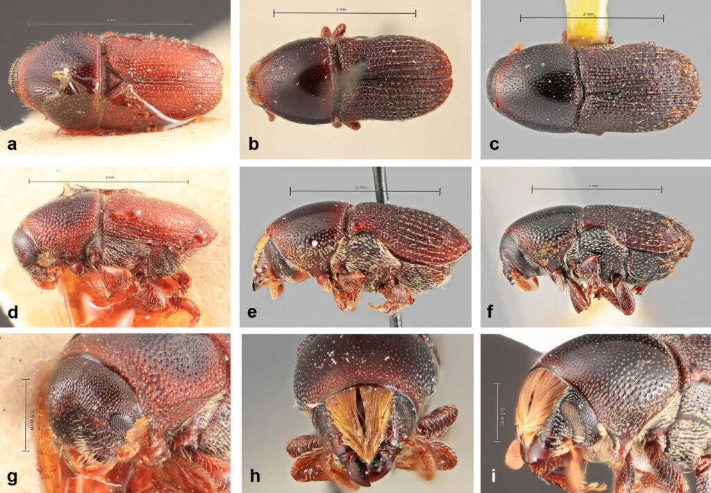
Figura 19. a, Vista dorsal de Scolytus rugulosus (tomada de Atkinson, 2025); b, vista dorsal de Scolytopsis toba (tomada de Atkinson, 2025); c, vista dorsal de S. punticollis (tomada de Atkinson, 2025); d, vista lateral de S. rugulosus (tomada de Atkinson, 2025); e, vista lateral de S. toba (tomada de Atkinson, 2025); f, vista lateral de S. punticollis (tomada de Atkinson, 2025); g, vista frontal de S. rugulosus (tomada de Atkinson, 2025); h, vista frontal de S. toba (tomada de Atkinson, 2025); i, vista frontal de S. punticollis (tomada de Atkinson, 2025).
Se diferencian por la presencia del tercer tarso de forma cilíndrica; ojos son emarginados; funículo antenal con 3-5 segmentos y maza puede presentar suturas y un único septo parcial; pubescencia del hipomeron está compuesta de setas simples raramente mezclado con setas bifurcadas; setas de interestrías similares a escamas; macho similar a la hembra, de tamaño más pequeño y no volador en Hypothenemus, generalmente hay dimorfismo sexual en la frente (Johnson et al., 2020).
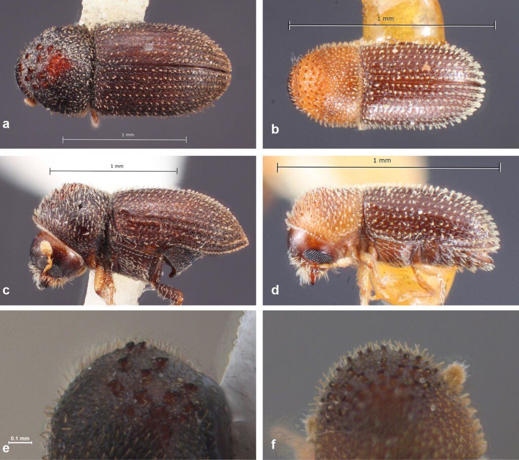
Figura 20. a, Vista dorsal de Hypothenemus meridensis (tomada de Atkinson, 2025); b, vista dorsal de H. eruditus (tomada de Atkinson, 2025); c, vista lateral de H. meridensis (tomada de Atkinson, 2025); d, vista lateral de H. eruditus (tomada de Atkinson, 2025); e, vista dorsal del pronoto de H. meridensis; f, vista dorsal del pronoto de H. eruditus.
Clave para las especies de la tribu Trypophloeini
1. Margen anterior del pronoto con 2 dientes (fig. 20e); pendiente anterior del pronoto con dientes gruesos elevados Hypothenemus meridensis,Wood
1’. Margen anterior del pronoto con 6 dientes (fig. 20f); pendiente anterior del pronoto con dientes medianos 2
2. Tamaño pequeño, 1.0- 1.3 mm; frente con superficie rugosa y reticulada; élitros con interestrías 2 veces más anchas que estrías Hypothenemus eruditus Westwood
2’. Tamaño del cuerpo de 1.4- 1.6 mm; frente rugosa y reticulada, con surco o tubérculo; élitros con estrías tan anchas como interestrías 3
3. Frente con tubérculo pequeño ubicado encima del nivel superior de ojos y surco poco profundo que se extiende desde el tubérculo hasta el epistoma (fig. 21e); declive elitral fuertemente convexo (fig. 21c) Hypothenemus crudiae (Panzer)
3’. Frente con surco poco profundo que llega hasta la tercera parte de distancia del margen del epistoma (fig. 21f); declive elitral convexo (fig. 21d) Hypothenemus seriatus (Eichhoff)
Hypothenemus meridensis Wood, 2007 (fig. 20a, c, e)
Distribución. Argentina: Tucumán; América del Sur: Brasil y Venezuela (Atkinson, 2025; Córdoba et al., 2023, 2025; Wood, 2007).
Hypothenemus eruditus Westwood, 1836 (fig. 20b, d, f)
Distribución. Argentina: Buenos Aires, Corrientes, Misiones, Santiago del Estero y Tucumán; América del Sur: Brasil, Colombia, Ecuador, Guyana, Trinidad y Tobago y Venezuela (Atkinson, 2025; Córdoba y Atkinson, 2018; Córdoba et al., 2021, 2023, 2025; Smith et al., 2017; Wood, 2007).
Hypothenemus crudiae (Panzer, 1791)* (fig. 21a, c, e)
Distribución. Argentina: Buenos Aires y Tucumán; América del Sur: Bolivia, Brasil, Colombia, Ecuador, Guyana, Paraguay, Surinam, Trinidad y Tobago y Venezuela (Atkinson, 2025; Atkinson y Flechtmann, 2021; Córdoba et al., 2023, 2025; Wood, 2007).
Comentarios. Esta especie se distribuye desde Estados Unidos hasta Argentina, también posiblemente introducida en Asia y África.
Hypothenemus seriatus (Eichhoff, 1872) (fig. 21b, d, f)
Distribución. Argentina: Tucumán; América del Sur: Bolivia, Brasil, Colombia, Ecuador, Paraguay, Perú y Venezuela (Atkinson, 2025; Córdoba et al., 2021, 2023, 2025; Smith et al., 2017; Wood, 2007).
Tribu Xyleborini LeConte, 1876
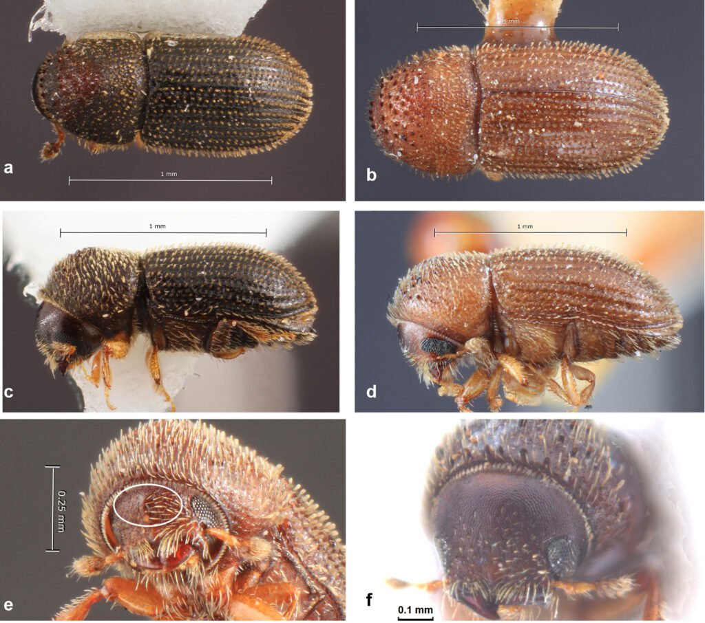
Figura 21. a, Vista dorsal de Hypothenemus crudiae (tomada de Atkinson, 2025); b, vista dorsal de H. seriatus (tomada de Atkinson, 2025); c, vista lateral de H. crudiae (tomada de Atkinson, 2025); d, vista lateral de H. seriatus (tomada de Atkinson, 2025); e, vista frontal de H. crudiae (tomada de Atkinson, 2025); f, vista frontal de H. seriatus.
Se caracterizan por presentar dimorfismo sexual marcado, macho generalmente más pequeño que hembra y no volador, ojo reducido en tamaño y haploide, la hembra normal y diploide; frente convexa, sin ornamentaciones; ojos son emarginados o divididos; frecuentemente escapo antenal alargado, funículo lleva 5 segmentos y maza antenal truncada de manera oblicua; parte anterior del pronoto empinada y armada con asperezas; procoxas varían de contiguas a ampliamente separadas; protibias expandidas, arqueadas y armadas con dentículos; escutelo puede ser grande y plano o modificado o ausente; en cuanto a su biología, la xilomicetofagia y la poligamia endogámica son universales en esta tribu (Wood, 2007).
Clave para las especies de la tribu Xyleborini
1. Declive de élitros abruptamente truncados con quilla circundeclivital, cara del declive ligeramente convexa con 3 estrías marcadas (fig. 22a, c, e); élitros tan largos como pronoto; procoxas contiguas (fig. 22g) Amasa parviseta Knížek et Smith
1’. Declive elitral aplanado o convexo, nunca truncado; élitros más largos que pronoto; procoxas contiguas o separadas 2
2. Escutelo en forma de espina y poco visible, dejando base de élitros con sutura hueca y cubierta de setas 3
2’. Escutelo en forma triangular y visible, concavidad sutural completamente llena hasta uperficie anterior de élitros, emarginación sin setas 5
3. Declive elitral convexo, empinado y débilmente impreso (fig. 22d, f); margen anterior del pronoto armado por dientes pequeños; longitud del cuerpo 1.9 a 2.4 mm Xyleborinus saxesenii (Ratzeburg)
3’. Declive elitral empinado e impreso; margen anterior del pronoto débilmente aserrado; longitud del cuerpo 2.0 a 2.6 mm 4
4. Frente reticulada, toscamente punteada (fig. 23e); longitud del cuerpo 2.0 a 2.2 mm y 2.9 más largo que ancho; declive elitral empinado e impreso hasta la sutura 3, con interestrías 1 y 2 impresas sin tubérculos, 3 débilmente elevada con 4 espinas (3 de mayor tamaño), intercaladas con otras más pequeñas, interestría 4 con tubérculos puntiagudos pequeños (fig. 23g) Xyleborinus linearicollis (Schedl)
4’. Frente reticulada con punciones gruesas y profundas (fig. 23f); longitud del cuerpo 2.3 a 2.6 mm y 3.2 veces más largo que ancho; declive elitral corto, muy empinado, fuertemente impreso desde la sutura hasta la interestría 3, interestría 1 con un tubérculo en la base, interestría 3 moderadamente elevada con 3 espinas grandes igualmente espaciadas (fig. 23h) Xyleborinus sentosus (Eichhoff)
5. Procoxas moderada o ampliamente separadas; pieza intercoxal continua, longitudinalmente sin emarginación 6
5’. Procoxas contiguas; pieza intercoxal longitudinalmente emarginada 7
6. Longitud del cuerpo 1.3 a 1.5 mm; coloración castaño oscura; pronoto más ancho en base, lados bastante convexos que convergen al ápice estrechamente redondeado, con mechón de setas ubicado longitudinalmente en la base del pronoto (fig. 24a, e); declive elitral brillante abruptamente redondeado en la base, con carena subserrada en el margen posterolateral, interestrías 2 y 3 con fila de pequeños tubérculos (fig. 24g) Xylosandrus curtulus (Eichhoff)
6’. Longitud del cuerpo 2.1 a 2.9 mm; coloración castaño rojiza; pronoto más ancho en base, lados poco convexos, con setas largas en los bordes y medianas en toda la superficie (fig. 24b, f); declive elitral opaco, muy convexo, densamente cubierto por pequeños gránulos uniforme e irregularmente distribuidos, con carena irregularmente dentada (fig. 24h) Xylosandrus crassiusculus Motschulsky
7. Tercio apical de cara posterior del maza antenal con 2 suturas, cara anterior con segundo segmento más grande, esclerotizado y levemente curvado (fig. 25e, g); cuerpo pequeño, robusto, convexo; longitud del cuerpo 1.8 a 2.1 mm; margen anterior del pronoto armado con 5 dientes medianos Coptoborus villosulus (Blandford)
7’. Tercio apical de cara posterior de maza antenal con 1 o sin suturas marcadas, cara anterior con segundo segmento, si es visible, no esclerotizado y fuertemente curvado (fig. 25f, h); cuerpo alargado, perfil muy levemente convexo a aplanado; longitud del cuerpo 2.0 a 3.2 mm; margen anterior de pronoto sin dientes 8
8. Pronoto subcuadrado (fig. 25b), margen anterior recto, superficie finamente estriada; longitud 2.2 a 2.5 mm; interestrías del declive elitral con filas de tubérculos de diferente tamaño Euwallacea posticus (Eichhoff)
8’. Pronoto más largo que ancho, margen anterior procurvado, superficie lisa; longitud 2.0 3.2 mm; interestrías del declive elitral con tubérculos o espinas 9
9. Declive elitral aplanado y brilloso 10
9’. Declive elitral convexo y opaco o brilloso 11
10. Especie pequeña, cuerpo delgado, longitud del cuerpo 2.0 a 2.9 (fig. 26a); frente con quilla débil ancha que se extiende en zona media, desde epistoma hasta ojos (fig. 26e); declive elitral suavemente empinado, interestría 3 con tubérculo mediano más cerca del ápice que de base del declive (fig. 24g) Xyleborus ferrugineus (Fabricius)
10’. Especie grande, cuerpo robusto, longitud del cuerpo 2.8 a 3.2 (fig. 24b); frente con quilla confinada a zona superior del epistoma (fig. 26f); declive elitral abrupto y empinado, interestría 3 con tubérculo mediano más cerca de base que del ápice del declive (fig. 26h) Xyleborus bispinatus Eichhoff
11. Frente con gránulos pequeños y dispersos (fig. 27e); declive elitral muy empinado y base abrupta (fig. 27c), interestría 1 con tubérculo grande ubicado sobre base protuberante en el tercio basal (fig. 27a, c, g) Xyleborus biconicus Eggers
11’. Frente reticulada sin gránulos; declive eitral con tubérculos pequeños o medianos en las interestrías (fig. 27h) 12
12. Frente fuertemente reticulada y de superficie opaca (fig. 27f); superficie del declive elitral opaca (fig. 27h) Xyleborus affinis Eichhoff
12’. Frente reticulada y de superficie brillante; superficie del declive elitral brillante (fig. 28g, h) 13
13. Frente toscamente reticulada, con línea media elevada y lisa desde el epistoma hasta el nivel superior de los ojos (fig. 28e); declive elitral con interestría 1 con 3 a 5 tubérculos puntiagudos y de tamaño mediano, interestría 2 con 2 o 3 tubérculos puntiagudos y medianos en el cuarto basal y 1 o 2 medianos cerca del ápice, interestría 3 con 3 tubérculos puntiagudos medianos muy espaciados entre sí en el 3 cuarto basal y 3 o más tubérculos pequeños en el cuarto basal (fig. 28g); margen ventrolateral del declive moderadamente elevado y con crenulaciones; coloración del cuerpo castaño rojizo Xyleborus volvulus (Fabricius)
13’. Frente fuertemente reticulada y sin elevaciones (fig. 28f); declive elitral con interestría 1 débilmente elevada, 2 y 3 con fila de tubérculos pequeños y de igual tamaño; coloración del cuerpo castaño rojizo muy oscuro Xyleborus scaber Schedl
Amasa parviseta Knížek et Smith, 2024* (fig. 22a, c, e, g)
Distribución. Argentina: Tucumán; América del Sur: Brasil y Uruguay (Atkinson, 2025; Córdoba et al., 2023, 2025; Flechtmann y Cognato, 2011; Gómez et al., 2017a; Knížek y Smith, 2024; Rainho et al., 2018)
Figura 22. a, Vista dorsal de Amasa parviseta (tomada de Atkinson, 2025); b, vista dorsal de Xyleborinus saxesenii (tomada de Atkinson, 2025); c, vista lateral de A. parviseta (tomada de Atkinson, 2025); d, vista lateral de X. saxesenii (tomada de Atkinson, 2025); e, vista posterior de A. parviseta (tomada de Atkinson, 2025); f, vista posterior de X. saxesenii (tomada de Atkinson, 2025); g, vista ventral de A. parviseta (tomada de Atkinson, 2025).
Comentarios. Es originaria de Australia y se extendió en asociación con especies introducidas de eucalipto. Se informó en Brasil (2015) (Rainho et al., 2018), Uruguay en 2015 (Gómez et al., 2017a), Chile en 2016 (Kirkendall, 2018) y Argentina en 2018 (Córdoba et al., 2023) como A. truncata y A. nr. truncata.
Xyleborinus saxesenii (Ratzeburg, 1837)* (fig. 22b, d, f)
Distribución. Argentina: Buenos Aires, Salta, Santiago del Estero y Tucumán; América del Sur: Brasil, Chile, Ecuador, Paraguay y Uruguay (Atkinson, 2025; Córdoba y Atkinson, 2018; Córdoba et al., 2021, 2023, 2025; Gómez et al., 2017a; Iturre y Darchuck, 1996; Wood, 2007).
Comentarios. Esta es una especie euroasiática y ha sido introducida en todas las regiones templadas y subtropicales del mundo.
Xyleborinus linearicollis (Schedl, 1937) (fig. 23a, c, e, g)
Distribución. Buenos Aires y Tucumán; América del Sur: Brasil (Atkinson, 2025; Córdoba et al., 2023, 2025; Wood, 2007).
Xyleborinus sentosus (Eichhoff, 1868) (fig. 23b, d, f, h)
Distribución. Argentina: Tucumán; América del Sur: Brasil, Paraguay y Perú (Atkinson, 2025; Córdoba et al., 2021, 2023, 2025; Smith et al., 2017; Wood, 2007).
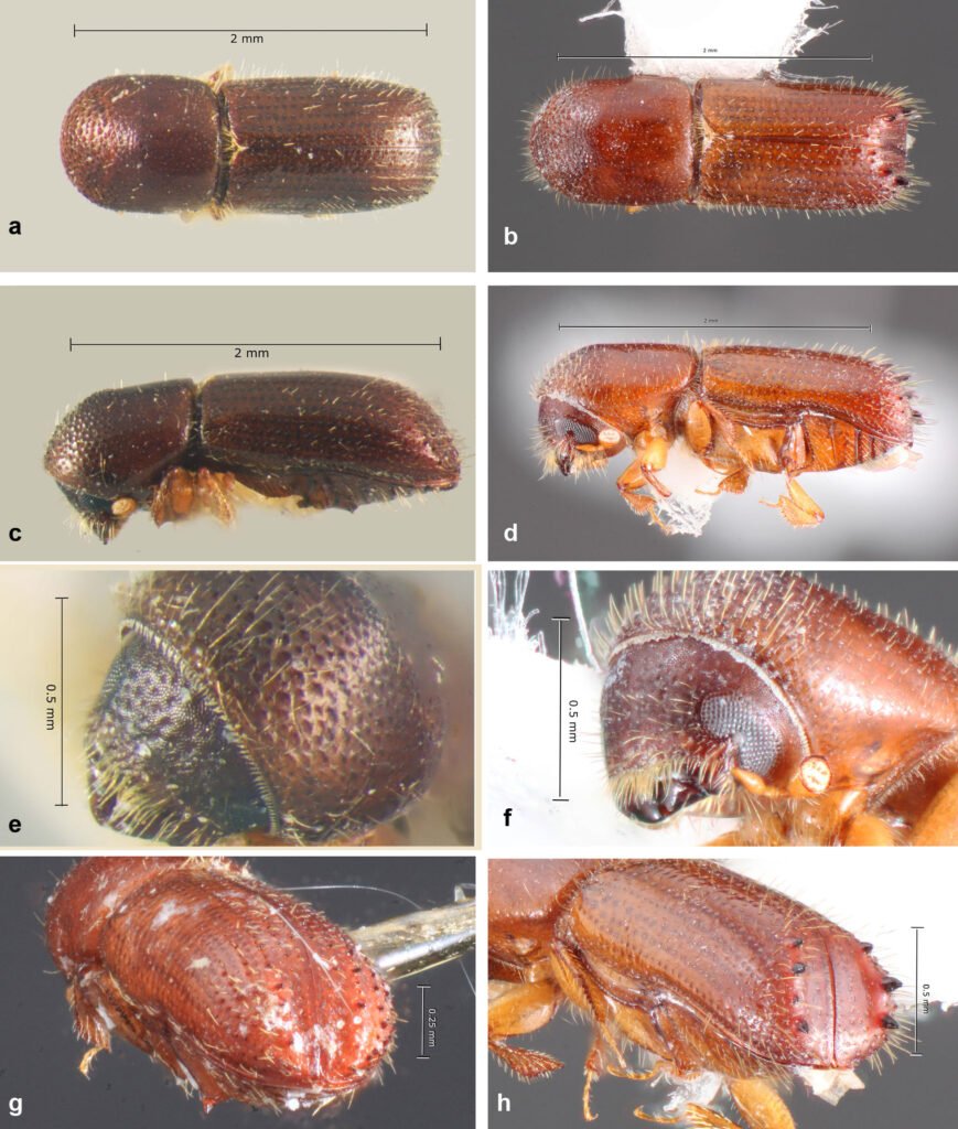
Figura 23. a, Vista dorsal de Xyleborinus linearicollis (tomada de Atkinson, 2025); b, vista dorsal de X. sentosus (tomada de Atkinson, 2025); c, vista lateral de X. linearicollis (tomada de Atkinson, 2025); d, vista lateral de X. sentosus (tomada de Atkinson, 2025); e, vista frontal de X. linearicollis (tomada de Atkinson, 2025); f, vista frontal de X. sentosus (tomada de Atkinson, 2025); g, vista posterior de X. linearicollis (tomada de Atkinson, 2025); h, vista posterior de X. sentosus (tomada de Atkinson, 2025).
Xylosandrus curtulus (Eichhoff, 1869) (fig. 24a, c, e, g)
Distribución. Argentina: Salta y Tucumán; América del Sur: Bolivia, Brasil, Colombia, Ecuador, Perú y Venezuela (Atkinson, 2025; Córdoba y Atkinson, 2018; Córdoba et al., 2021, 2023, 2025; Martínez et al., 2019; Smith et al., 2017; Wood, 2007).
Xylosandrus crassiusculus Motschulsky, 1866* (fig. 24b, d, f, h)
Distribución. Argentina: Buenos Aires y Tucumán; América del Sur: Brasil, Guyana Francesa y Uruguay (Atkinson, 2025; Landi et. al., 2017; Córdoba y Atkinson, 2018; Córdoba et al., 2021, 2023, 2025; Martínez et al., 2019).
Comentarios. Probablemente es originaria de Asia tropical y subtropical, pero se ha extendido ampliamente en regiones cálidas y húmedas de todo el mundo.
Coptoborus villosulus (Blandford, 1898) (fig. 25a, c, e, g)
Distribución. Argentina: Tucumán; América del Sur: Bolivia, Brasil, Colombia, Ecuador, Guyana Francesa, Perú, Trinidad y Tobago y Venezuela (Atkinson, 2025; Córdoba y Atkinson, 2018; Córdoba et al., 2021, 2023, 2025; Smith y Cognato, 2021; Wood, 2007).
Euwallacea posticus (Eichhoff, 1869) (fig. 25b, d, f, h)
Distribución. Misiones y Tucumán; América del Sur: Bolivia, Brasil, Colombia, Ecuador, Guyana, Paraguay, Perú, Surinam, Trinidad y Tobago y Venezuela (Atkinson, 2018; Atkinson, 2025; Córdoba y Atkinson, 2018; Córdoba et al., 2021, 2023, 2025; Wood, 2007).
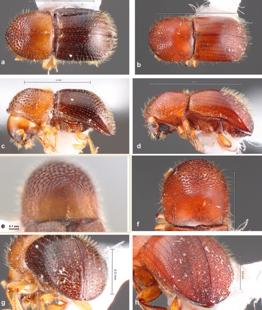
Figura 24. a, Vista dorsal de Xylosandrus curtulus (tomada de Atkinson, 2025); b, vista dorsal de X. crassiusculus (tomada de Atkinson, 2025); c, vista lateral de X. curtulus (tomada de Atkinson, 2025); d, vista lateral de X. crassiusculus (tomada de Atkinson, 2025); e, detalle pronoto de X. curtulus; f, detalle pronoto de X. crassiusculus (modificada de Atkinson, 2025); g, vista posterior de X. curtulus (tomada de Atkinson, 2025); h, vista posterior de X. crassiusculus (tomada de Atkinson, 2025).
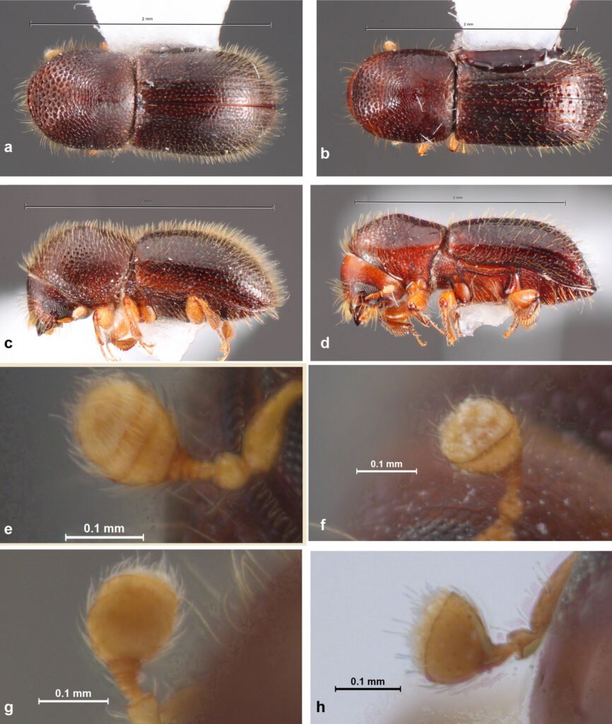
Figura 25. a, Vista dorsal de Coptoborus villosulus (tomada de Atkinson, 2025); b, vista dorsal de Euwallacea posticus (tomada de Atkinson, 2025); c, vista lateral de C. villosulus (tomada de Atkinson, 2025); d, vista lateral de E. posticus (tomada de Atkinson, 2025); e, vista posterior de la antena de C. villosulus; f, vista posterior de la antena de E. posticus; g, vista anterior de la antena de C. villosulus; h, vista anterior de la antena de E. posticus.
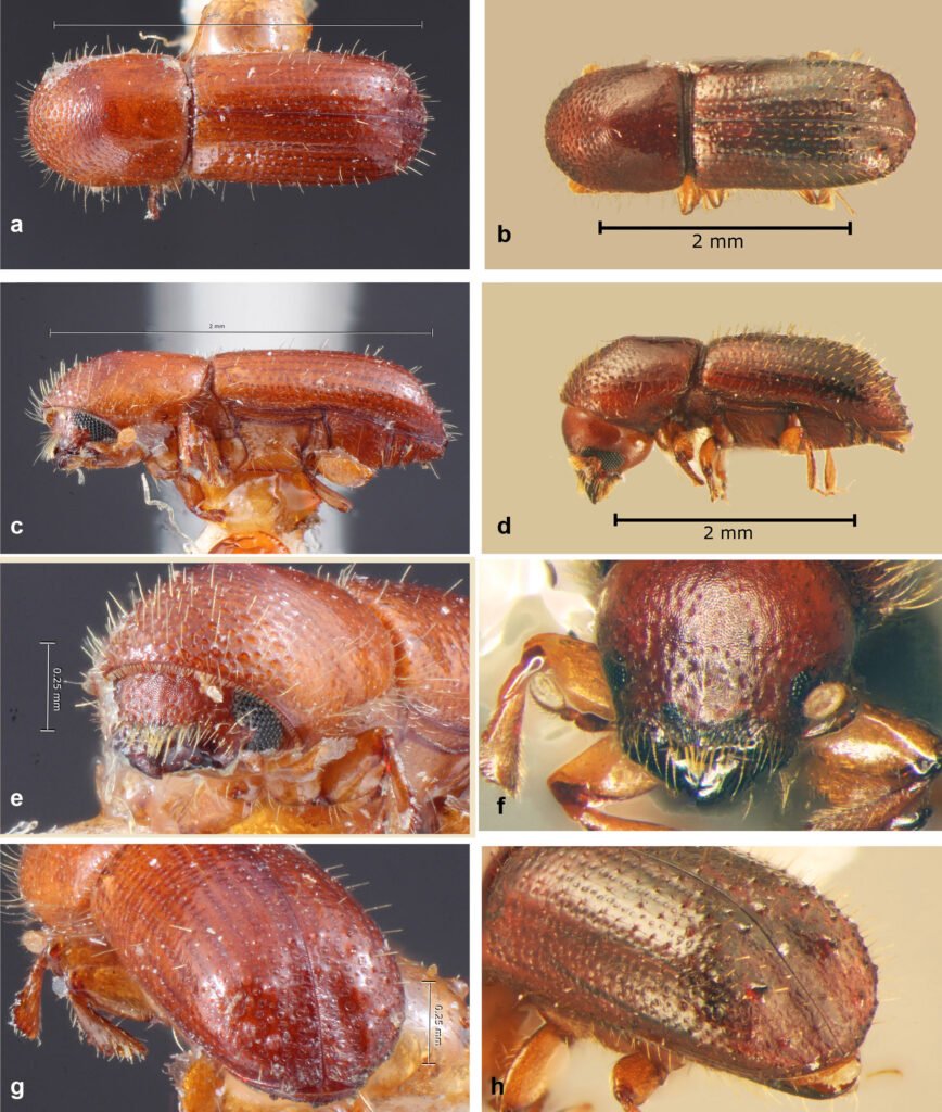
Figura 26. a, Vista dorsal de Xyleborus ferrugineus (tomada de Atkinson, 2025); b, vista dorsal de X. bispinatus (tomada de Atkinson, 2025); c, vista lateral de X. ferrugineus (tomada de Atkinson, 2025); d, vista lateral de X. bispinatus (tomada de Atkinson, 2025); e, vista frontal de X. ferrugineus (tomada de Atkinson, 2025); f, vista frontal de X. bispinatus (tomada de Atkinson, 2025); g, vista posterior de X. ferrugineus (tomada de Atkinson, 2025); h, vista posterior de X. bispinatus (tomada de Atkinson, 2025).
Xyleborus ferrugineus (Fabricius, 1801) (fig. 26a, c, e, g)
Distribución. Argentina: Jujuy, Salta y Tucumán. América del Sur: Bolivia, Brasil, Chile, Colombia, Ecuador, Guyana Francesa, Guyana, Paraguay, Perú, Surinam, Trinidad y Tobago, Uruguay y Venezuela (Atkinson, 2025; Córdoba y Atkinson, 2018; Córdoba et al., 2021, 2023, 2025; Martínez et al., 2019; Smith et al., 2017; Atkinson, 2025).
Xyleborus bispinatus Eichhoff, 1868 (fig. 26b, d, f, h)
Distribución. Argentina: Tucumán; América del Sur: Bolivia, Brasil, Colombia, Ecuador, Guyana Francesa, Paraguay, Perú, Surinam, Trinidad y Tobago y Venezuela (Atkinson, 2025; Córdoba et al., 2021, 2023, 2025; Martínez et al., 2019; Smith et al., 2017).
Xyleborus biconicus Eggers, 1928 (fig. 27a, c, e, g)
Distribución. Argentina: Formosa y Misiones, Tucumán; América del Sur: Bolivia, Brasil, Guyana Francesa y Paraguay (Atkinson, 2025; Córdoba et al., 2023, 2025; Wood, 2007).
Xyleborus affinis Eichhoff, 1868 (fig. 27b, d, f, h)
Distribución. Argentina:Jujuy, Misiones, Salta y Tucumán; América del Sur: Bolivia, Brasil, Chile, Colombia, Ecuador, Guyana Francesa, Guyana, Paraguay, Perú, Surinam, Trinidad y Tobago, Uruguay y Venezuela (Atkinson, 2025; Córdoba y Atkinson, 2018; Córdoba et al., 2021, 2023, 2025; Martínez et al., 2019; Smith et al., 2017).
Xyleborus volvulus (Fabricius, 1775)* (fig. 28a, c, e, g)
Distribución. Argentina:Jujuy yMisiones; América del Sur: Bolivia, Brasil, Colombia, Ecuador, Guyana Francesa, Guyana, Paraguay, Perú, Surinam, Trinidad y Tobago, Uruguay y Venezuela (Atkinson, 2025; Córdoba y Atkinson, 2018; Córdoba et al., 2021, 2023, 2025; Martínez et al., 2019; Smith et al., 2017; Wood, 2007).
Xyleborus scaber Schedl, 1949 (fig. 28b, d, f, h)
Distribución. Argentina: Tucumán; América del Sur: Brasil (Atkinson, 2025; Córdoba et al., 2023, 2025).
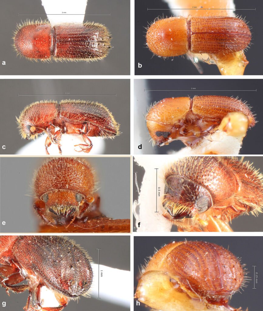
Figura 27. a, Vista dorsal de Xyleborus biconicus (tomada de Atkinson, 2025); b, vista dorsal de X. affinis (tomada de Atkinson, 2025); c, vista lateral de X. biconicus (tomada de Atkinson, 2025); d, vista lateral de X. affinis (tomada de Atkinson, 2025); e, vista frontal de X. biconicus (tomada de Atkinson, 2025); f, vista frontal de X. affinis (tomada de Atkinson, 2025); g, vista posterior de X. biconicus (tomada de Atkinson, 2025); h, vista posterior de X. affinis (tomada de Atkinson, 2025).
Discusión
Atkinson (2025) enumera 199 especies de Scolytinae para la Argentina. De estas especies, 56 están presentes en Tucumán, lo cual representa aproximadamente 31% de las especies conocidas de la subfamilia para el país. Consideramos que esta cifra es muy baja en comparación con la fauna de otras regiones neotropicales. El número de especies tucumanas coincide con la abundancia de especies de la tribu Xyleborini documentadas en todo el territorio mexicano, siendo esta tribu uno de los grupos más diversos a nivel mundial (Pérez-Silva et al., 2021).
La diversidad de especies en la provincia de Tucumán, comparada con los países limítrofes ubicados aproximadamente a la misma latitud (Chile, Paraguay y Uruguay) es alta, ya que Atkinson (2025) reporta 52 especies para Chile, 46 para Paraguay y 14 para Uruguay. En Argentina, 10% de las especies son introducidas, mientras que en Uruguay más de la mitad (57%) son especies exóticas. Esto se debe al incremento de terrenos destinados a la plantación de especies forestales arbóreas en Uruguay y al crecimiento del comercio internacional, en particular el intercambio de embalajes de madera, lo que facilita el establecimiento de especies exóticas (Gómez et al, 2017b). En la provincia de Tucumán, 12% son especies introducidas, lo que puede deberse al bajo porcentaje de superficie forestal. La mayoría de estas especies fueron recolectadas en ambientes naturales, son especies establecidas en el país y su origen foráneo está bien documentado (Wood, 1982, 2007).
Figura 28. a, Vista dorsal de Xyleborus volvulus (tomada de Atkinson, 2025); b, vista dorsal de X. scaber (tomada de Atkinson, 2025); c, vista lateral de X. volvulus (tomada de Atkinson, 2025); d, vista lateral de X. scaber (tomada de Atkinson, 2025); e, vista frontal de X. volvulus (tomada de Atkinson, 2025); f, vista frontal de X. scaber (tomada de Atkinson, 2025); g, vista posterior de X. volvulus (tomada de Atkinson, 2025); h, vista posterior de X. scaber (tomada de Atkinson, 2025).
Aunque Wood (2007) realizó una revisión de los Scolytinae para América del Sur, donde se incluyen especies presentes en Argentina, las nuevas especies, los recientes registros y los cambios taxonómicos hacen necesarias claves actualizadas. Además, no se cuenta con claves para la identificación a nivel más local, para la provincia y el país. Uno de los problemas principales de la clave de tribus de Wood (2007) es que intenta seguir sus ideas sobre la filogenia de los grupos y muchas veces ignora características sencillas, empleando algunas más difíciles de interpretar. Como consecuencia, muchos de sus dilemas son demasiado largos y complejos, dificultando su interpretación. Otro problema es que sigue estrictamente un concepto dicotómico sin presentar una matriz de caracteres que esconde similitudes para el reconocimiento. Por ejemplo, en todos los géneros de la tribu Scolytini, la cabeza está descubierta en vista dorsal a pesar de la impresión que presenta la clave en el primer dilema. Hay otros ejemplos que se pueden citar. Aquí hemos intentado usar caracteres menos ambiguos, sin considerar su supuesto valor filogenético.
Las presentes claves taxonómicas, que incorporan los cambios, especies recientemente descritas y nuevos registros, constituyen una importante herramienta para la identificación rápida de las especies de Argentina y América del Sur, lo cual puede ser de gran utilidad en casos de invasión de los cultivos o para futuras investigaciones.
Agradecimientos
A Eduardo Agustín Mendoza (Área Biología Integrativa, Fundación Miguel Lillo) por su valiosa colaboración y asistencia en todas las colectas en el campo. A Pablo Pereyra (Instituto de Iconografía, Área de Zoología, Fundación Miguel Lillo) por su contribución en la toma de fotografías y edición de las mismas.
Referencias
Atkinson, T. H. (2017). Familia Curculionidae: Scolytinae y Platypodinae. En T. D. Cibrián (Ed.), Fundamentos de entomología forestal (pp. 269–278). Texcoco: Universidad Autónoma de Chapingo.
Atkinson, T. H. y Flechtmann, C. A. H. (2021). New species, new records and synonymy of Brazilian species of Hypothenemus Westwood, 1834 (Coleoptera: Curculionidae: Scolytinae). Insecta Mundi, 846, 1–33. https://doi.org/10.11646/zootaxa.4442.2.11
Atkinson, T. H. (2025). Bark and ambrosia beetles of the Americas. Recuperado el 21 marzo, 2025 de: http://www.barkbeetles.info
Bachman, A. O. y Lanteri, A. A. (2013). Catalog of the types of Curculionoidea (Insecta: Coleoptera) deposited at the Museo Argentino de Ciencias Naturales ‘Bernardino Rivadavia’, Buenos Aires. Revista del Museo Argentino de Ciencias Naturales, 15, 209–280. https://doi.org/10.22179/revmacn.15.183
Bosq, J. M. (1943). Segunda lista de coleópteros de la República Argentina dañinos a la agricultura (reedición de Ingeniería Agronómica, IV, 18–22, Buenos Aires 1942). Revista del Ministerio de Agricultura de la Nación, Dirección de Sanidad Vegetal, 4, 1–80.
Bruch, C. (1914). Catálogo sistemático de los coleópteros de la República Argentina, Pars VII. Revista del Museo de La Plata, 19, 401–441. https://doi.org/10.5962/bhl.title.8799
Córdoba, S. P. y Atkinson, T. H. (2018). New records of Scolytinae (Coleoptera: Curculionidae) from Argentina. The Coleopterists Bulletin, 72,376–379. https://doi.org/10.1649/0010-065x-72.2.376
Córdoba, S. P., Mendoza, E. A., Atkinson T. H. y Manzo, M. V. (2021). Diversidad y dinámica poblacional de Scolytinae (Coleoptera: Curculionidae) en plantaciones de palto y bosque natural circundante en el NW de Argentina. Dugesiana, 28, 115–130. https://doi.org/10.32870/dugesiana.v28i2.7151
Córdoba, S. P., Atkinson, T. H. y Mendoza, E. A. (2023). Checklist of the subfamily Scolytinae (Coleoptera: Curculionidae) in Tucumán province, Argentina. Zootaxa, 5353,501–532. https://doi.org/10.11646/zootaxa.5353.6.1
Córdoba, S. P., Atkinson, T. H. y Mendoza, E. A. (2025). Listado preliminar de Scolytinae (Coleoptera: Curculionidae) de la provincia de Tucumán (adiciones y correcciones) y sus plantas hospedantes de Argentina. Dugesiana, 32, 13–38. https://doi.org/10.32870/dugesiana.v32i1.7357
Costilla, M. A. y Coronel, N. B. (1994). El taladillo de la semilla del palto Pagiocerus fiorii Eggers, 1940 (Bostrichus frontalis Fbricius, 1801) (Coleoptera: Scolytidae). Revista Industrial y Agrícola de Tucumán, 71, 63–68.
Flechtmann, C. A. H. y Cognato, A. I. (2011). First report of Amasa truncata (Erichson) (Coleoptera: Curculionidae: Scolytinae) in Brazil. Coleopterists Bulletin, 65,417–421. https://doi.org/10.1649/072.065.0419
Gómez, D., Suárez, M. y Martínez, G. (2017a). Amasa truncata (Erichson) (Coleoptera: Curculionidae: Scolytinae): A new exotic ambrosia beetle in Uruguay. Coleopterists Bulletin, 71, 825–826. https://doi.org/10.1649/0010-065x-71.4.825
Gómez, D., Irigoyen, A., Balmelli, G., Viera, C. y Martínez, G. (2017b). Patterns in flight phenologies of bark beetles (Coleoptera: Scolytinae) in commercial pine tree plantations in Uruguay. Bosque, 38, 47–53. https://doi.org/10.4067/s0717-92002017000100006
Hayward, K. J. (1960). Insectos tucumanos perjudiciales. Revista Industrial y Agrícola de Tucumán, 42, 3–144.
Hulcr, J., Atkinson, T. H., Cognato, A. I., Jordal, B. H. y McKenna, D. D. (2015). Morphology, taxonomy and phylogenetics of bark beetles. En F. E. Vega y R. W. Hofstetter (Eds.), Bark beetles: biology and ecology of native and invasive species (pp. 41–84). New York: Species Academic Press. https://doi.org/10.1016/b978-0-12-417156-5.00002-2
Iturre, M. y Darchuck, E. (1996). Registro de escolítidos relacionados al género Eucalyptus en Santiago del Estero. Quebracho, 4, 11–16.
Johnson, A. J., Hulcr, J., Knížek, M., Atkinson, T. H., Mandelshtam, M. Y., Smith, S. M. et al. (2020). Revision of the bark beetle genera within the former Cryphalini (Curculionidae: Scolytinae). Insect Systematics and Diversity, 4, 1–81. https://doi.org/10.1093/isd/ixaa002
Jordal, B. H. y Smith, S. M. (2020). Scolytodes Ferrari (Coleoptera, Scolytinae) from Ecuador: 40 new species, and a molecular phylogenetic guide to infer species differences. Zootaxa, 4813, 1–67. https://doi.org/10.11646/zootaxa.4813.1.1
Kirkendall, L. R. (2018). Invasive bark beetles (Coleoptera, Curculionidae, Scolytinae) in Chile and Argentina, including two species new for South America, and the correct identity of the Orthotomicus species in Chile and Argentina. Diversity, 10, 2–20. https://doi.org/10.3390/d10020040
Kirkendall, L. R. y Jordal, B. H. (2006). Revision of the bark beetle genera within the former Cryphalini (Curculionidae: Scolytinae). Taxonomy, 4,1–81.
Kirkendall, L. R., Biederman, P. H. W. y Jordal, B. H. (2015). Evolution and diversity of bark and ambrosia beetles. En F. E. Vega y R. W. Hofstetter (Eds.), Bark beetles: Biology and ecology of native and invasive species (pp. 85–156). Cambridge, USA: Academic Press. https://doi.org/10.1016/b978-0-12-417156-5.00003-4
Knížek, M. y Smith, S. M. (2024). A new widely distributed invasive alien species of Amasa ambrosia beetles (Coleoptera: Curculionidae: Scolytinae: Xyleborini). Zootaxa, 5403,385–390. https://doi.org/10.11646/zootaxa.5403.3.8
Landi, L., Gómez, D., Braccini, C. L, Pereyra, V. A., Smith, S. M. y Marvaldi, A. E. (2017). Morphological and molecular identification of the Invasive Xylosandrus crassiusculus (Coleoptera: Curculionidae: Scolytinae) and its South American range extending into Argentina and Uruguay. Annals of the Entomological Society of America, 110, 344–349. https://doi.org/10.1093/aesa/sax032
Lombardero, M. J. (1995). Plantas huésped y escolítidos (Col.: Scolytidae) en Galicia (noroeste de la península Ibérica). Boletín de Sanidad Vegetal. Plagas, 21,357–370.
Martínez, M., Cognato, A. I., Guachambala, M. y Boivin, T. (2019). Bark and ambrosia beetles (Coleoptera: Curculioni-
dae: Scolytinae) diversity in natural and plantation forests
in Ecuador. Environmental Entomology, 48,603–613. https://doi.org/10.1093/ee/nvz037
Morris, J. L., Cottrell, S., Fettig, C. J., Hansen, W. D., Sherriff, R. L., Carter, V. A. et al. (2018). Managing bark beetle impacts on ecosystems and society: Priority questions to motivate future research. Frontiers in Ecology and the Environment, 16, 34–43. https://doi.org/10.1002/fee.1754
Pérez-De la Cruz, M., Hernández-May, M. A., De la Cruz-Pérez, A. y Sánchez-Soto, S. (2016). Scolytinae y Platypodinae (Coleoptera: Curculionidae) de dos áreas de conservación en Tabasco, México. Biología Tropical, 64,319–326. https://doi.org/10.15517/rbt.v64i1.15931
Pérez-Silva, M., Equihua-Martínez, A., Atkinson, T. H., Romero-Nápoles, J. y López-Buenfil, J. A. (2021). Claves ilustradas para la identificación de géneros y especies de la tribu Xyleborini (Curculionidae: Scolytinae) de México. Revista Mexicana de Biodiversidad, 92, e923817. https://doi.org/10.22201/ib.20078706e.2021.92.3817
Petrov, A. V. (2017). New data on Scolytini Latreille, 1804, mainly from Peru, with description of two new species of Cnemonyx Eichhoff, 1868 (Coleoptera: Curculionidae: Scolytinae). Koleopterologische Rundschau, 87, 325–334. https://doi.org/10.31857/s0367144523020119
Rainho, H. L., Silva, W. D., Leite, M. O. G. y Bento, J. M. S. (2018). Notes on the distribution of the exotic ambrosia beetle Amasa truncata (Erichson) (Coleoptera: Curculionidae: Scolytinae) in southeastern Brazil. Coleopterists Bulletin, 72, 870–872. https://doi.org/10.1649/0010-065x-72.4.870
Santoro, F. H. (1966). Panorama entomológico relacionado con la Silvicultura y la tecnología forestal en la República Argentina. Revista Forestal Argentina, 10, 52–59.
Smith, S. M., Petrov, A. V. y Cognato, A. I. (2017). Beetles (Coleoptera) of Peru: a survey of the familie (Curculionidae: Scolytinae). The Coleopterists Bulletin, 71, 77–94. https://doi.org/10.1649/0010-065x-71.1.77
Smith, S. M. y Cognato, A. I. (2021). A revision of the Neotropical genus Coptoborus Hopkins (Coleoptera, Curculionidae, Scolytinae, Xyleborini). Zookeys, 1044, 609–720. https://doi.org/10.3897/zookeys.144.62246
Viana, M. J. (1964). Datos ecológicos de Scolytidae argentinos (Coleoptera). Revista de la Sociedad Entomológica Argentina, 27, 119–130.
Wood, S. L. (2007). Bark and ambrosia beetles of South America (Coleoptera, Scolytidae). Monte L. Brigham Young University, Provo, Utah: Bean Life Science Museum. https://doi.org/10.1134/s001387380902016x
Wood, S. L. (1982). The bark and ambrosia beetles of North and Central America (Coleoptera: Scolytidae), a Taxonomic Monograph. Great Basin Naturalist Memoirs, 6, 1–1359.
Wood, S. L. y Bright, D. E. (1992). A catalog of Scolytidae and Platypodidae (Coleoptera), Part 2: Taxonomic index, volumes A and B. Provo, Utah: Great Basin Naturalist Memoirs.

Propagación in vitro y adaptación de plantas a condiciones ex vitro de Kroenleinia grusonii (Cactaceae)
In vitro propagation and adaptation of plants to ex vitro conditions of Kroenleinia grusonii (Cactaceae)
Dolores Adilene García-González, Juan Pedro Flores-Margez y Pedro Osuna-Ávila *
Universidad Autónoma de Ciudad Juárez, Instituto de Ciencias Biomédicas, Av. Benjamín Franklin Núm. 4650, Zona Pronaf Condominio La Plata, 32310 Ciudad Juárez, Chihuahua, México
*Autor para correspondencia: posuna@uacj.mx (P. Osuna-Ávila)
Recibido: 23 mayo 2025; aceptado: 14 octubre 2025
Resumen
Kroenleinia grusonii (Hildm.) Lodé, es una cactácea endémica del centro de México que enfrenta riesgos como la colecta ilegal o la modificación de su hábitat natural y se encuentra catalogada como en peligro de extinción. El objetivo de este trabajo fue evaluar concentraciones de 6-bencilaminopurina (BAP) sola o combinada con ácido indolacético (AIA) en la formación de brotes de K. grusonii e inducir la formación de raíces para valorar la adaptación de plantas a condiciones ex vitro. La inducción de brotes fue con BAP (0, 1.0, 2.0 y 3.0 mg/L), AIA (0.5 mg/L) y BAP (0, 1.0, 2.0 y 3.0 mg/L) + AIA (0.5 mg/L). Se aplicó AIA 0, 1.0, 2.0 y 3.0 mg/L para enraizamiento y la adaptación ex vitro de las plantas fue con musgo de turba y con una mezcla de musgo de turba y suelo natural (1:1). El mejor tratamiento fue BAP 3.0 mg/L con 5.13 ± 0.9150 brotes por explante. Se obtuvo 89 ± 0.03% de brotes enraizados y la sobrevivencia ex vitro fue de 68.75% en musgo de turba con suelo natural (1:1). Se estableció un protocolo para la propagación clonal de K. grusonii, lo cual representa una contribución para su conservación ex situ.
Palabras clave: Ácido indol-3-acético; 6-bencilaminopurina; Brotes; Cactus; Endémica; Enraizamiento
Abstract
Kroenleinia grusonii (Hildm.) Lodé, is a cactus endemic to central Mexico, that faces risks such as illegal collection or modification of its natural habitat and is listed as endangered. The objective of this work was to evaluate different concentrations of 6-benzylaminopurine (BAP) alone or combined with indoleacetic acid (IAA) in K. grusonii and to induce root formation to assess plant adaptation to ex vitro conditions. Shoot induction was with BAP (0, 1.0, 2.0 and 3.0 mg/L), IAA (0.5 mg/L) and BAP (0, 1.0, 2.0 and 3.0 mg/L) + IAA (0.5 mg/L). AIA 0, 1.0, 2.0 and 3.0 mg/L was applied for rooting and the ex-vitro adaptation of the plants was with peat moss and a mix with peat moss with natural soil (1:1). The best treatment was BAP 3.0 mg/L with 5.13 ± 0.9150 shoots per explant. 89 ± 0.03% of rooted shoots were obtained and the ex-vitro survival was 68.75% in peat moss substrate with natural soil (1:1). A protocol for the clonal propagation of K. grusonii was established, which represents a contribution to its ex-situ conservation.
Keywords: Indole-3-acetic acid; 6-bencylaminoourine; Shoots; Cactus; Endemic; Rooting
Introducción
Kroenleinia grusonii (Hildm.) Lodé (Cactaceae), también conocida como la biznaga barril de oro, es una especie que se utiliza con fines ornamentales, gastronómicos y agropecuarios (Rodríguez et al., 2021). La especie se distribuye principalmente en el centro de México en los estados de Guanajuato, Querétaro, Hidalgo, San Luis Potosí y Zacatecas (Lodé, 2014). Se encuentra en riesgo de desaparecer debido a la destrucción de su hábitat natural, ya que sus poblaciones se encuentran en deterioro por la colecta ilegal, el desarrollo urbano y la construcción de carreteras, entre otros factores (Pérez-Molphe-Balch et al., 2015; Villavicencio-Gutiérrez et al., 2023). Kroenleinia grusonii es un taxón endémico y debido a las adversidades que enfrenta, se encuentra enlistado en la NOM-059-SEMARNAT-2010 bajo la categoría en peligro de extinción (Semarnat, 2019). La UICN (Unión Internacional para Conservación de la Naturaleza) la cataloga como especie en peligro (Guadalupe-Martínez et al., 2013). En consecuencia, es necesario implementar estrategias que permitan la propagación de esta especie para su conservación y protección sin afectar a las poblaciones naturales.
La propagación de las cactáceas se realiza, principalmente, mediante semillas; sin embargo, es necesario buscar otras formas (Manzo et al., 2022), en particular, cuando las especies se encuentran bajo algún estatus de riesgo y no es posible obtener suficientes semillas para iniciar protocolos de propagación (Pérez-Molphe-Balch et al., 2015). Una alternativa es el uso de herramientas biotecnológicas, como el cultivo de tejidos vegetales. Con esta técnica es posible la propagación clonal manteniendo la estabilidad genética clonal y obtener un gran número de plantas con fines de conservación ex situ (Torres-Silva et al., 2021).
Esta herramienta ofrece obtener una rápida multiplicación vegetativa comparado con la propagación tradicional (Mabrouk et al., 2021). Con esta técnica biotecnológica se reduciría el impacto que se ha creado en las cactáceas debido a la sobrecolecta (López-Granero et al., 2021). La técnica se basa en la totipotencia celular que incluye la expresión total del genoma presente en la célula, que permite la multiplicación aumentando el número de individuos (Almeida et al., 2021). Esta cualidad se ve incrementada por la adición de reguladores de crecimiento en el medio de cultivo, especialmente las citoquininas y auxinas, que favorecen el desarrollo de nuevos brotes (Civatti et al., 2017). El potencial regenerativo de las plantas puede variar dependiendo de diversos factores, como el genotipo, el explante utilizado y los reguladores de crecimiento (Torres-Silva et al., 2018).
En cactáceas se ha realizado la propagación in vitro utilizando diferentes explantes como lo son plantas adultas de Opuntia ficus-indica (L.) Mil. (Khalafalla et al., 2007), activación de areolas en Turbinicarpus pseudomacrochele subsp. lausseri (Diers et G. Framk) Glass (de la Rosa-Carrillo et al., 2012), secciones transversales o longitudinales de plántulas de Melocactus glaucescens Buining et Brederoo (Torres-Silva et al., 2018) o brotes como en Echinocactus parryi Engelm. (García-González et al., 2020). Un paso fundamental en el proceso de propagación in vitro es la formación de raíces en los brotes obtenidos (Ivannikov et al., 2022). La inducción de raíces se logra con el uso de auxinas o en ocasiones, sin la necesidad de aplicarlas (Martínez et al., 2016). Por ejemplo, en la cactácea Cereus peruvianus (L.) Mill. los brotes regenerados obtuvieron 100% de enraizamiento en medio de cultivo MS (Murashige y Skoog, 1962) al 25% sin auxinas (Sawsan et al., 2004). Los brotes enraizados son transferidos a condiciones de invernadero, que es la última etapa de la propagación in vitro (Jagiello-Kubiec et al., 2021). El objetivo de la presente investigación fue evaluar diferentes concentraciones de 6-bencilaminopurina (BAP), sola o combinada con ácido indolacético (AIA) en la formación de nuevos brotes de K. grusonii; así como inducir en los brotes la formación de raíces y evaluar 2 sustratos para su adaptación a condiciones ex vitro.
Materiales y métodos
Para la inducción de brotes, se utilizaron plántulas de 90 días de cultivo in vitro de Kroenleinia grusonii como fuente de explantes, que se obtuvieron de experimentos de germinación in vitro de semillas (Osuna-Ávila et al., 2025). A las plántulas se les eliminó la raíz y se utilizaron los ápices completos, los cuales se colocaron en medio de cultivo MS a una concentración de 100% de macro y micronutrientes. El medio de cultivo se suplementó con 30g/L de sacarosa, 7 g/L de agar tipo 1 y el pH se ajustó a 5.7 ± 0.1. Posteriormente, se adicionaron diferentes concentraciones de BAP, AIA y AIA + BAP. Los tratamientos utilizados fueron 8 y consistieron en lo siguiente: control, BAP 1.0, 2.0 y 3.0 mg/L, combinada con o sin AIA. La unidad experimental fue un frasco de 100 ml conteniendo de 20-25 ml del medio de cultivo con 3 repeticiones, se colocaron 5 explantes en cada frasco con 15 explantes por tratamiento y un total de 120 unidades experimentales. Los explantes fueron subcultivados 2 veces en las mismas condiciones cada 60 días. El número total de brotes por cada explante fue registrado después de 120 días de cultivo in vitro.
Los brotes obtenidos de la propagación clonal fueron separados de los explantes utilizando pinzas y se colocaron en medio de cultivo MS al 100% adicionado con diferentes concentraciones de AIA. Los tratamientos fueron 4 y consistieron en lo siguiente: control, AIA 1.0, 2.0 y 3.0 mg/l. La unidad experimental fue el frasco de 100 ml conteniendo 20-25 ml de medio de cultivo con 8 repeticiones, se colocaron aleatoriamente 10 brotes en cada frasco para un total de 80 brotes en cada tratamiento y 320 unidades experimentales. El porcentaje de formación de raíces se evaluó después de 90 días de cultivo in vitro.
Para la adaptación de las nuevas plantas a condiciones ex vitro, se procedió a retirarlas del medio de cultivo utilizando los dedos para ablandar el agar y posteriormente enjuagando las raíces con agua de la llave. A los brotes que formaron raíces, se les midió la longitud de la raíz primaria utilizando un vernier digital y se contaron el número de raíces que se formaron en la base del brote. Se utilizaron 2 sustratos, el primero fue musgo de turba y el segundo fue una mezcla de musgo de turba y suelo natural regosol con textura franco arcillosa, pH de 8 y conductividad eléctrica de 0.45 dS m-1 (IUSS-WRB, 2015) (proporción 1:1). Cada sustrato fue colocado en una charola de 54 cm × 27 cm con 128 cavidades, en donde se colocaron los brotes que formaron raíces. Las plantas se regaron cada 24 h con agua de la llave a capacidad de campo, manteniendo humedad constante del sustrato. Después de 30 días en condiciones ex vitro se evaluó el porcentaje de sobrevivencia.
El análisis de datos fue realizado con el programa estadístico SPSS versión 24.0 (IBM. 2017). Se aplicó la prueba de Kruskal-Wallis no paramétrica para muestras independientes (prueba X²), ya que se trataba de variables discretas (número de brotes y raíces) y de una variable continua (longitud de raíz). La comparación múltiple de promedios se llevó a cabo con la prueba de Bonferroni con un nivel de significancia de 0.05 y los estadísticos descriptivos fueron obtenidos.
Resultados
El número de brotes por explante fue significativamente diferente entre los tratamientos aplicados (p < 0.05). Los mejores resultados de brotación fueron con BAP 3.0 mg/L (fig. 1A), seguido por BAP 1.0 mg/L + AIA 0.5 mg/L (fig. 1B) con un promedio de brotes de 5.13 por explante en cada uno después de 120 días de cultivo in vitro. Cuando el BAP 3.0 mg/L se combinó con AIA 0.5 mg/L, el número de brotes se redujo a 3.6 ± 0.914 (tabla 1). Los resultados no fueron significativos en el grupo control con un promedio de 0.07 ± 0.067 brotes por explante y el AIA 0.5 mg/L con 0.40 ± 0.400 brotes por explante. Los tratamientos de BAP 1.0 mg/L, BAP 2.0 mg/L, AIA 0.5 mg/l + BAP 2.0 mg/L y AIA 0.5 mg/L + BAP 3.0 mg/L, formaron brotes; sin embargo, no fueron significativos con promedios desde 2.8 hasta 3.6 brotes por explante (tabla 1). Los nuevos brotes obtenidos, presentaron diferentes tamaños desde 5 hasta 18 mm de diámetro (fig. 1C).
Tabla 1
Número de brotes obtenidos en la propagación clonal de Kroenleinia grusonii a los 120 días de cultivo in vitro (n = 15).
| BAP mg/L | AIA mg/L | Número de brotes |
| 0 (control) | 0 | 0.07 ± 0.067 b |
| 1.0 | 0 | 3.20 ± 0.890 ab |
| 2.0 | 0 | 3.13 ± 2.109 ab |
| 3.0 | 0 | 5.13 ± 0.9150 a |
| 0 | 0.5 | 0.40 ± 0.400 b |
| 1.0 | 0.5 | 5.13 ± 1.055 a |
| 2.0 | 0.5 | 2.80 ± 1.010 ab |
| 3.0 | 0.5 | 3.60 ± 0.914 ab |
Medias ± el error estándar, letras iguales no son estadísticamente diferentes (n = 80).
Tabla 2
Porcentaje de enraizamiento de brotes, número de raíces por brote y longitud de la raíz principal a los 90 días de cultivo in vitro de Kroenleinia grusonii.
| AIA mg/L | % de enraizamiento | Número de raíces | Longitud de raíces (mm) |
| Control | 66 ± 0.05 b | 3.21 ± 0.385 b | 21.86 ± 1.764 a |
| 1.0 | 77 ± 0.04 ab | 2.89 ± 0.255 b | 19.98 ± 1.631 a |
| 2.0 | 89 ± 0.03 a | 4.68 ± 0.407 a | 22.36 ± 1.583 a |
| 3.0 | 84 ±0.04 a | 3.18 ± 0.293 b | 22.24 ± 1.688 a |
Medias ± el error estándar, letras iguales no son estadísticamente diferentes (n = 80).
La tabla 2 indica que hubo diferencias entre los tratamientos para el porcentaje de inducción de raíces en los brotes cultivados in vitro por 90 días. Para el porcentaje de enraizamiento, se observó que el adicionar AIA al medio de cultivo MS promueve significativamente la formación de raíces en los brotes. Particularmente, con el tratamiento de AIA 2.0 mg/L que resultó ser el mejor con 89 ± 0.03 % de enraizamiento, en comparación con el tratamiento control que mostró 66 ± 0.05 % de brotes enraizados (tabla 2). Por tales motivos, el aplicar AIA 2.0 mg/L resulta ser, aproximadamente, 20% más efectivo para la inducción de raíces que el resto de los tratamientos.
El número de raíces por explante fue significativamente diferente entre tratamientos (p < 0.05). La comparación de promedios muestra que el AIA 2.0 mg/L presentó el mayor promedio de número de raíces con aproximadamente 5 (4.68 ± 0.407) en cada brote. Mientras que el AIA 1.0 mg/L, AIA 2.0 mg/L y el control desarrollaron, en promedio, menos de 3.2 raíces por explante (tabla 2; fig. 2).
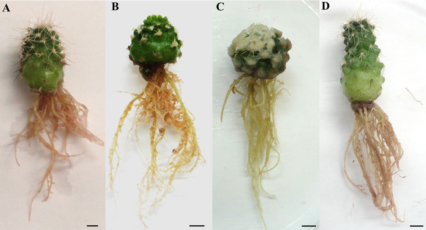
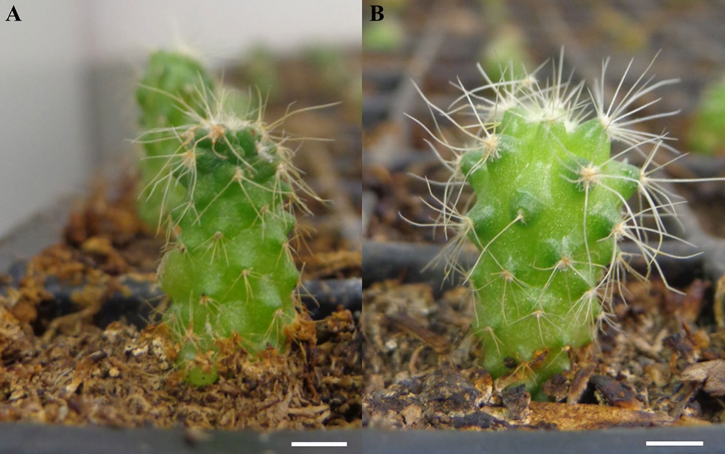
En relación con la variable largo de raíz, no se detectó efecto significativo (p = 0.604). El intervalo observado entre los tratamientos fue de 2.38 mm en promedio, es decir, la variable mostró poca variación. Sin embargo, por los resultados obtenidos con AIA 2.0 mg/L, se muestra un promedio ligeramente por arriba que el resto de los tratamientos con 22.36 ± 1.583 mm (tabla 2). Después de 60 días en condiciones ex vitro, el mejor sustrato para promover la aclimatización de las plantas fue el de suelo de turba y suelo natural (1:1). El porcentaje de sobrevivencia que presentó este sustrato fue de 68.75% después de 60 días. Mientras que el sustrato de suelo de turba mostró un porcentaje de sobrevivencia inferior, de 60.93% después de 60 días (fig. 3).
Discusión
La conservación ex situ de cactáceas a través de la propagación clonal es una alternativa viable para las especies que se encuentran en alguna situación de riesgo (Torres-Silva et al., 2021). Con el uso de citoquininas, en algunas cactáceas que no forman brotes laterales, se rompe la dominancia apical y se promueve la formación de nuevos brotes (Lema-Ruminska y Kulus, 2014). Particularmente, con los resultados observados, el uso de BAP 3.0 mg/l promovió la misma cantidad de brotes que la combinación de BAP 1.0 mg/l y AIA 0.5 mg/l, lo cual indica que para obtener resultados significativos no sería necesaria la adición de auxinas al medio de cultivo. Ramírez y Salazar (2016) reportan que la cinetina 10 mg/l es más eficiente en la formación de brotes en los explantes que al combinarla con auxina en Mammillaria petterssonii Hildm. y Coryphanta radians (D. C). Britton et Rose. El resultado es similar en Stenocereus stellatus al utilizar BAP 4.0 mg/L y obtener un promedio de 8 brotes por explante (Martínez et al., 2011). Por el contrario, existen especies que han sido propagadas y que para obtener mayor formación de brotes sí requieren una combinación de citoquinina y auxina. Por ejemplo, en M. geminispina Haw. con cinetina 10 mg/l + AIA 4.0 mg/l obtuvieron 6 brotes por explante (Ramírez y Salazar, 2016). Melocactus glaucescens Buining et Brederoo con BAP 4.0 mg/l + ácido 1-naftalenacético (ANA) 0.25 mg/l presentó 2.5 brotes por explante y sin ANA, un promedio de 0.6 (Torres-Silva et al., 2018). En Echinocactus parryi reportan que es más efectiva la combinación de BAP 2.0 mg/l + AIA 0.5 mg/l al regenerar 2.9 brotes por explante, a diferencia de los tratamientos sin AIA en los que el número de brotes no fue significativo (García-González et al., 2020).
Una consideración importante en Kroenleinia grusonii es que el número de brotes se redujo de 5.13 ± 0.9150 obtenidos con BAP 3 mg/l a 3.6 ± 0.914 al combinar el BAP 3.0 mg/l + AIA 0.5 mg/l. Resultados similares se reportaron para Coryphantha retusa (Pfeiff.) Birtton et Rose, ya que al aplicar BAP 2.0 mg/l el promedio de brotes fue de 8.8 por explante y al combinar BAP 2.0 mg/l + ANA 1.0 mg/l el número de brotes se redujo a 4.2 (Ruvalcaba-Ruíz et al., 2010). Lo mismo sucedió con Pachycereus pringlei (S. Watson) Britton et Rose, con BAP 2.0 mg/l el número de brotes fue de 3.8 ± 0.3 y se redujo a 0.6 ± 0.1 al combinarlo con ANA 0.5 mg/l (Pérez-Molphe-Balch et al., 2002). Los resultados que se obtengan en la propagación clonal dependen del genotipo y de los reguladores de crecimiento utilizados (Montiel-Frausto et al., 2016).
Es de gran importancia establecer un sistema de micropropagación específico para cada especie, no obstante, la respuesta a la formación de raíces y la aclimatización ex vitro puede variar debido a las condiciones de cultivo (Elias et al., 2015). Con los resultados obtenidos en K. grusonii, el tratamiento control mostró una respuesta favorable a la formación de raíces en los brotes. Sin embargo, al utilizar AIA 2.0 mg/l, se logra 30% más de enraizamiento, lo cual significa que se pueden obtener 70 plantas completas. El porcentaje de enraizamiento en K. grusonii se podría considerar alto con la aplicación de AIA debido a que se han reportado porcentajes inferiores de enraizamiento en diferentes especies de cactáceas. Algunos ejemplos son Cereus jamacaru DC. con 70% (Monostori et al., 2012) o Mammillaria vetula subsp. gracilis (Pfeiff.) D. R. Hunt con 20% de enraizamiento (López-Granero et al., 2021). El uso de auxinas como el ácido indolbutírico (AIB) 0.1 mg/l en Hylocereus monacanthus (Hort. ex Lem.) Britton et Rose donde el porcentaje fue mayor que en K. grusonii con 100% de enraizamiento (Montiel-Frausto et al., 2016). En contraste, para diferentes especies y con medios de cultivo sin auxinas, se ha logrado obtener hasta 95% de enraizamiento en C. retusa (Ruvalcaba-Ruíz et al., 2010), Micranthocereus flaviflorus Buining et Brederoo con 98% (Civatti et al., 2017), Mammillaria hernandezii Glass et R. A. Foster con 98.4% de enraizamiento y Mammillaria dixanthocentron Beckeb. ex Mottram con 94% (Lázaro-Castellanos et al., 2018) comparados con los reportados en la presente investigación para K. grusonii.
El uso de AIA 2.0 mg/l es la mejor opción para obtener el mayor número y longitud de raíces en K. grusonii. Resultados similares han sido reportados para H. monacanthus, donde el número de raíces obtenidas en los brotes presentó un promedio de 4.2 por planta, aunque la longitud de la raíz fue aproximadamente 6 veces menor a la de K. grusonii con 3.6 mm (Montiel-Frausto et al., 2016). También Turbinicarpus × mombergeri Říha presentó raíces de menor longitud que las de K. grusonii con 13 mm (Santos-Díaz et al., 2021). En cuanto al porcentaje de sobrevivencia de las plantas aclimatizadas, es importante resaltar que es necesario implementar métodos más eficientes para lograr aumentar el porcentaje de sobrevivencia de las plantas. Ejemplo de ello fue el trabajo realizado por Santos-Díaz et al. (2021), en donde la sobrevivencia de plantas de Turbinicarpus × mombergeri fue de 85% después de 1 año. Otro ejemplo sobresaliente fue lo mostrado por Cortés-Olmos et al. (2023), al reportar 100% de sobrevivencia en plantas de Gymnocalycium cv Fancy. De acuerdo con los resultados obtenidos y con base en literatura consultada, se infiere que las respuestas entre especies pueden llegar a ser muy diferentes, por lo cual se confirma que es necesario establecer protocolos específicos para cada especie y poder aprovechar al máximo el potencial regenerativo de cada una.
Se ha establecido un protocolo de la propagación clonal de Kroenleinia grusonii que inicia con la inducción de brotes, posteriormente el enraizamiento y finaliza con la aclimatización ex vitro. Con los resultados obtenidos en K. grusonii se logró la formación de hasta 5 brotes más con el uso de BAP 3.0 mg/l. Al inducir la formación de raíces en los brotes regenerados, es viable obtener aproximadamente 3 plantas nuevas por cada explante utilizado en la fase de inducción de brotes. Esta información representa un avance para continuar implementando técnicas de propagación in vitro en K. grusonii y que en futuras investigaciones se pueda promover un mayor número de plantas. Los resultados de este estudio, podrían contribuir a los programas de conservación ex situ e in situ de K. grusonii.
Referencias
Almeida, C. V. T., Amorim, D. S. E. P. y da Cunha, R. A. C. (2021). 5 medium MS at different concentrations in the initial development in vitro of Melocactus conoideus Buining & Brederoo. Scientia, 6, 81–91.
Civatti, L. M., Marchi, M. N. G., Schnadelbach, A. S. y Bellintani, M. C. (2017). In vitro multiplication and genetic stability of two species of Micranthocereus Backeb. (Cactaceae) endemic to Bahia, Brazil. Plant Cell, Tissue and Organ Culture, 131, 537–545. https://doi.org/10.1007/s11240-017-1304-6
Cortés-Olmos, C., Guerra-Sandoval, V. M., Blanca-Giménez, V. y Rodríguez-Burruezo, A. (2023). Micropropagation and acclimatization of Gymnocalycium cv. Fancy (Cactaceae): developmental responses to different explant types and hormone conditions. Plants, 12, 3932. https://doi.org/10.3390/plants12233932
de la Rosa-Carrillo, M. L., Domínguez-Rosales, M. S., Pérez-Reyes, M. E. y Pérez-Molphe-Balch, E. (2012). Cultivo y propagación in vitro de cactáceas amenazadas del género Turbinicarpus. Interciencia, 37, 114–120.
Elias, H., Mat, T. R., Hasbullah, N. A., Mohamed, N., Manan, A. A., Mahmad, N. et al. (2015). The effects of plant growth regulators in shoot formation, regeneration and coloured callus production in Echinocereus cinerascens in vitro. Plant Cell, Tissue and Organ Culture, 120, 729–739. https://doi.org/10.1007/s11240-014-0642-x
García-González, D. A., Santos-Díaz, M. S., Flores-Margez, J. P. y Osuna-Ávila, P. (2020). Influencia del Ca2+, pH, agar y reguladores de crecimiento en la propagación in vitro de Echinocactus parryi (Engelm). Terra Latinoamericana, 38, 489–498. https://doi.org/10.28940/terra.v38i3.734
Guadalupe-Martínez, G. J., Cárdenas, N. R. y Hernández, O. D. B. (2013). Echinocactus grusonii. The IUCN Red List of Threatened Species 2013: e.T40962A2947851. Recuperado el 29 septiembre, 2025 de: https://dx.doi.org/10.2305/IUCN.UK.2013-1.RLTS.T40962A2947851.en
IBM. (2017). IBM SPSS Estatistics for Windows, version 24.0. IBM Corp. Armonk, USA.
IUSS-WRB (International Union of Soil Sciences-World Reference Base for Soil Resources). (2015). World Reference Base for Soil Resources 2014. Update 2015 International soil classification system for naming soils and creating legends for soil maps. World Soil Resources Reports No. 106. FAO, Rome. Recuperado el 26 septiembre, 2025 de: http://www.fao.org/3/i3794en/I3794en.pdf.
Ivannikov, R., Lobova, O., Ivannikova, N. y Krasnienkova, I. (2022). Micropropagation and organogenesis of Astrophytum asterias (Zucc.) Lem. (Cactaceae Juss.), Blossfeldia liliputiana Werdem. and Strombocactus disciformis (DC.) Britton y Rose. Journal of Microbiology, Biotechnology and Food Sciences, 11, e2201. https://doi.org/10.55251/jmbfs.2201
Jagiello-Kubiec, K., Nowakowska, K., Lukaszewska, A. J. y Pacholczak, A. (2021). Acclimation to ex vitro conditions in ninebark. Agronomy, 11, 612. https://doi.org/10.3390/agronomy11040612
Khalafalla, M. M., Abdellatef, E., Mohameed, A. M. M. y Osman, M. G. (2007). Micropropagation of cactus (Opuntia ficus-indica) as strategic tool to combat desertification in arid and semi arid regions. International Journal of Sustainable Crop Production, 2, 1–8.
Lázaro-Castellanos, J. O., Mata-Rosas, M., González, D. Arias, S. y Reverchon, F. (2018). In vitro propagation of endangered Mammillaria genus (Cactaceae) species and genetic stability assessment using SSR markers. In Vitro Cellular & Developmental Biology – Plant, 54, 518–529. https://doi.org/10.1007/s11627-018-9908-z
Lema-Ruminska, J. y Kulus, D. (2014). Micropropagation of cacti- a review. Haseltonia, 19, 46–63. http://dx.doi.org/10.2985/026.019.0107
Lodé, J. (2014). Kroenleinia gen. nov. J. Lodé: a new genus for a well-known cactus: Echinocactus grusonii. International Cactus Adventures, 102, 25–29.
López-Granero, M., Arana, A., Regalado, G. J. J. y López, E. C. (2021). In vitro mass micropropagation of Mammillatia vetula ssp. gracillis var. Arizonica snowcap. Plant Cell, Tissue and Organ Culture, 155, 759–771. https://orcid.org/10.21203/rs.3.rs-738336/v1
Mabrouk, A., Abbas, Y., El Goumi, Y., El Maaiden. E., El kharrassi, Y., El Antry-Tazi, S. et al. (2021). Optimization of prickly pear cacti (Opuntia spp.) micropropagation using an experimental design method. Journal of Microbiology, Biotechnology and Food Sciences, 11, 1–7. https://doi.org/10.15414/jmbfs.1577
Manzo, R. M. S., González, R. H., García, S. G., García-Moya, E., Espinosa-Hernández, V., Corona, T. T. et al. (2022). Viabilidad y germinación de semillas de cuatro especies amenazadas de cactáceas. Caldasia, 44, 209–220. https://doi.org/10.15446/caldasia.v44n2.86192
Martínez, P. A., Cárdenas, N. R. y Hernández, O. D. B. (2016). Micropropagation of endemic Turbinicarpus valdezianus (Möeller) Glass y Foster (Cactaceae) an endemic cactus in northern Mexico. Horticultural Science, 51, 94–97.
https://doi.org/10.21273/HORTSCI.51.1.94
Martínez, V. Y. M., Andrade, R. M. Villegas, M. A., Tejal, I. A., Villegas, T. O. G. y López, M. V. (2011). Cultivo in vitro del pitayo (Stenocereus stellatus (Pfeiffer) Riccobono). Revista Chapingo Serie Horticultura, 17, 95–105.
Monostori, T., Tanács, L. y Mile, L. (2012). Studies on in vitro propagation methods in cactus species of the genera Melocactus, Cereus and Lobivia. Acta Horticulturae, 937, 255–261. https://doi.org/10.17660/ActaHortic.2012.937.31
Montiel-Frausto, L. B., Enríquez, V. J. R. y Aroldo, C. (2016). Propagación in vitro de Hylocereus monacanthus (Lem.) Britton y Rose. Biotecnología Vegetal, 16, 113–123.
Murashige, T. y Skoog, F. (1962). A revised medium for rapid growth and bioassays with tobacco tissue cultures. Physiologia Plantarum, 15, 473–497. https://doi.org/10.1111/j.1399-3054.1962.tb08052.x
Osuna-Ávila, P., Florez-Margez, J. P. y García-González, D. A. (2025). Efecto de tratamientos pregerminativos y peso de las semillas en la germinación in vitro de Kroenleinia grusonii (Cactaceae). Acta Botanica Mexicana, 132, 2414. https://doi.org/10.21829/abm132.2025.2414
Pérez-Molphe Balch, E., Santos-Díaz, M. S., Ramírez-Malagón, R. y Ochoa-Alejo, N. (2015). Tissue culture of ornamental cacti. Scientia Agricola, 72, 540–561. http://doi.org/10.1590/0103-9016-2015-0012
Pérez-Molphe Balch, E., Pérez-Reyes, M. E., Dávila-Figueroa, C. A. y Villalobos-Amador, E. (2002). In vitro propagation of three species of columnar cacti from the Sonoran Desert. Horticultural Sciences, 37, 639–696. https://doi.org/10.21273/HORTSCI.37.4.693
Ramírez, M. R. y Salazar, S. E. (2016). Propagación y conservación in vitro de siete especies de cactáceas del noreste del estado de Guanajuato. Acta Universitaria Multidisciplinary Scientific Journal, 26, 78–82. áhttp://doi.org/10.15174/au.2016.1540
Rodríguez, A. S. P., Muñoz, O. A., Durán, F. R., Hernández, F. J. Limón, M. J. P. y Hernández-Hernández, H. M. (2021). Micropropagación como alternativa para evitar la extinción de plantas endémicas. Journal of Bioengineering and Biomedicine Research, 5, 1–15.
Ruvalcaba-Ruíz, D., Rojas-Bravo, D. y Valencia-Botín, A. J. (2010). Propagación in vitro de Coryphantha retusa (Britton y Rose) un cactus endémico y amenazado. Tropical and Subtropical Agroecosystems, 12, 139–143.
Santos-Díaz, M. S., Santos-Díaz, M. L. y Alvarado-Rodríguez, J. (2021). In vitro regeneration of the endangered cactus Turbinicarpus mombergeri Riha, a hybrid of T. laui × T. pseudopectinatus. Plant Cell, Tissue and Organ Culture, 148, 271–279. https://doi.org/10.1007/s11240-021-02181-5
Sawsan, S. S. Abou-Dahab, T. A. y Youssef, E. M. A. (2004). In vitro propagation of cactus (Cereus peruvianus L.). Arab Journal of Biotechnology, 8, 196–176.
Semarnat (Secretaría de Medio Ambiente y Recursos Naturales). (2019). Modificación del Anexo Normativo III, Lista de especies en riesgo de la Norma Oficial Mexicana NOM- 059-SEMARNAT-2010, Protección ambiental-Especies nativas de México de flora y fauna silvestres-Categorías de riesgo y especificaciones para su inclusión, exclusión o cambio-Lista de especies en riesgo. Publicada el 30 de diciembre de 2010. Diario Oficial de la Federación. Cd. Mx., México. Recuperado el 25 septiembre, 2025 de: https://www.dof.gob.mx/nota_detalle.php?codigo=5578808&fecha=14/11/2019#gsc.tab=0
Torres-Silva, G., Resende, S. V., Lima-Brito, A., Bezerra, H. B., De Santana, J. R. F. y Schnadelbach, A. S. (2018). In vitro shoot production, morphological alterations and genetic instability of Melocactus glaucescens (Cactaceae), an endangered species endemic to eastern Brazil. South African Journal of Botany, 115, 100–107. https://doi.org/10.1016/j.sajb.2018.01.001
Torres-Silva, G., Selbach, S. A., Basile, B. H., Lima-Brito, A. y Vitória, R. S. (2021). In vitro conservation and genetic diversity of threatened species of Melocactus (Cactaceae). Biodiversity and Conservation, 30, 1067–1080. https://doi.org/10.1007/s10531-021-02132-8
Villavicencio-Gutiérrez, E. E., Quintana-Camargo, M., Sánchez-Barra, F., Cano-Pineda, A. y Ríos-Saucedo, J. C. (2023). Calidad de semillas de dos biznagas del género Echinocactus Tribu Cacteae (Fam.: Cactaceae). Agrofaz, Journal of Environmental and Agroecological Sciences, 5, 8–15.

Genetic diversity of Oenothera drummondii (Onagraceae),a dune coastal herb: ecological and evolutionary implications
Diversidad genética de Oenothera drummondii (Onagraceae), una herbácea de dunas costeras: implicaciones ecológicas y evolutivas
Raquel Aurora Hernández-Espinosa a, Jorge González-Astorga a, *,
Yessica Rico b, Juan B. Gallego-Fernández c
a Instituto de Ecología A.C., Red de Biología Evolutiva, Laboratorio de Genética de Poblaciones, Carretera Antigua a Coatepec No. 351, El Haya, 91073 Xalapa, Veracruz, Mexico
b Instituto de Ecología A.C., Centro Regional del Bajío, Red de Diversidad Biológica del Occidente Mexicano, Av. Lázaro Cárdenas No. 253, 61600 Centro, Pátzcuaro, Michoacán, Mexico
c Universidad de Sevilla, Departamento de Biología Vegetal y Ecología, Av. de la Reina Mercedes, 6, 41012 Sevilla, Spain
*Corresponding author: jorge.gonzalez@inecol.mx (J. González-Astorga)
Received: 09 June 2025; accepted: 31 October 2025
Abstract
We studied the diversity and genetic structure of Oenothera drummondii Hook. (Onagraceae), a dune plant with a mixed reproductive system, across 9 populations using 10 microsatellite markers. Plant genetic diversity is governed by intrinsic factors (i.e., reproductive system and dispersal) and extrinsic factors (i.e., population fluctuations and founder effects). We found moderate to low genetic diversity, with southern populations showing lower diversity, and northern populations higher. A separate study on self-compatibility revealed higher selfing in the south and lower in the north, suggesting a latitudinal gradient that may reduce genetic diversity in southern populations. Peripheral populations showed reduced diversity and greater differentiation, likely due to increased isolation and limited gene flow. Central populations near the Texas origin exhibited the highest diversity. Populations from Baja California (O. drummondii subsp. thalassaphila) formed a genetically distinct group, suggesting a separate species. Overall, genetic patterns in O. drummondii genetic diversity reflect historical and ecological influences, including mating system variation, floral traits, and pollinator dynamics. These findings support hypotheses such as center-periphery dynamics and climate-driven historical processes (e.g., post-glacial expansion), which may shape the species’ genetic landscape and suggest possible local adaptations to environmental changes.
Keywords: Neutral genetic diversity; Coastal dunes; Microsatellites; Genetic bottleneck; Latitude; Selfing
Resumen
Evaluamos la diversidad y estructura genética de Oenothera drummondii Hook. (Onagraceae), planta de dunas costeras con sistema reproductivo mixto; se usaron 9 poblaciones y 10 marcadores microsatélites. La diversidad genética en plantas está influenciada por factores intrínsecos (dispersión y sistema reproductivo) y factores extrínsecos (fluctuaciones poblacionales y efecto fundador). Encontramos diversidad genética moderada a baja, con menor diversidad en poblaciones del sur (Ojoshal) y mayor en el norte (Bolívar). Un estudio complementario mostró mayor autocompatibilidad en Ojoshal y menor en Bolívar, sugiriendo un gradiente latitudinal con incremento de autocompatibilidad hacia el sur, con posible reducción de diversidad genética. Las poblaciones periféricas presentaron menor diversidad y mayor diferenciación, asociada a menor flujo génico y mayor aislamiento; las poblaciones centrales, cercanas al origen de la especie en Texas, mostraron mayor diversidad. Las poblaciones de Baja California (O. drummondii subsp. thalassaphila) formaron un grupo genético distinto, que podría representar a una especie separada. En conjunto, los patrones genéticos de O. drummondii reflejan procesos históricos y ecológicos relacionados con el sistema reproductivo, características florales y las dinámicas de polinización, lo cual podría significar adaptaciones locales a cambios ambientales, y patrones de distribución genética asociados con ellos, como la hipótesis de centro-periferia.
Palabras clave: Diversidad genética neutral; Dunas costeras; Microsatélites; Cuellos de botella; Latitud; Autocompatibilidad
Introduction
Genetic diversity may be considered a crucial factor in determining the ability of populations to adapt and evolve, thus increasing their evolutionary potential (He et al., 2024). Understanding the drivers of genetic variation among plant populations is essential in evolutionary biology as this diversity is the foundation for adaptive potential and long-term survival (Chung et al., 2023; Wright, 1969). In plants, the factors that shape genetic variation can be divided into: a) intrinsic biological properties (e.g., the genetic recombination system, including ploidy level, reproductive system, and meiotic behavior; the mode of dispersal and pollination; and the life form), and b) extrinsic dynamic processes (e.g., fluctuations in population size due to bottlenecks, founder effect, invasions, and changes caused by ecological succession) (Duminil et al., 2009). The reproductive system is the intrinsic biological property suggested to be the major driver of genetic diversity in plants (i.e., heterozygosity and population genetic differentiation) (Koelling et al., 2011; Wright, 1969), as it influences the mating patterns within a population by determining the extent to which selfing can occur (Charlesworth, 2006; Raduski et al., 2012). Self-incompatible populations, for instance, are composed of outcrossing plants with a predominantly outcrossing mating system. Conversely, in partially or completely self-compatible plants, the mating system can span from outcrossing to mixed mating to complete selfing (Holsinger, 1991).
Small, low-density populations experiencing habitat fragmentation and isolation, with limited mate or pollinator availability, exhibit increased propensity for self-fertilization (Devaux et al., 2014; Whitehead et al., 2018). In situations where self-fertilization is evolutionarily advantageous, selection will favor changes in traits that facilitate selfing (e.g., reductions in flower size, reduced nectar, pollen and reduced herkogamy) (Opedal, 2018; Shimizu & Tsuchimatsu, 2015; Sicard & Lenhard, 2011). These changes can have consequences at the genetic level, including elevated rates of inbreeding, a reduction in genetic diversity within populations, and increased genetic differentiation among populations (Barrett & Harder, 1996; Ingvarsson, 2002). Furthermore, a principal consequence of predominant self-fertilization is the reduction in heterozygosity and intra-population genetic diversity, coupled with an increase in inter-population differentiation, when compared to self-incompatible plants (Hamrick & Godt, 1996). In contrast, clonal species are expected to exhibit higher levels of heterozygosity than self-incompatible species, but lower levels of polymorphism within the population and higher levels of differentiation between populations (Levin, 2012).
In addition to the intrinsic biological properties of the species, spatial distribution and demography strongly influence processes such as genetic drift, gene flow, and natural selection, which in turn shape the genetic characteristics of populations (Eckert et al., 2008). For example, species range size tends to influence gene flow and genetic differentiation between populations. Large distances between populations with large ranges would be barriers to gene flow (Lawrence & Fraser, 2020). Peripheral populations are predicted to exhibit reduced gene flow, greater isolation, and higher genetic differentiation. In contrast, populations in the center of the distribution would have higher gene flow and be less differentiated (Lawrence & Fraser, 2020). This may be exacerbated if the peripheral populations experience rapid cycles of colonization and extinction, and have associated bottleneck events or founder effects (Eckert et al., 2008). Dispersal ability also influences the amount of gene flow between core and peripheral populations. This has implications for the maintenance of genetic diversity. For example, species with large ranges but limited mobility have reduced gene flow between populations, resulting in greater genetic differentiation (Pelletier & Carstens, 2018).
The genus Oenothera (Onagraceae) is widespread with the majority of species concentrated in western North America (Overson et al., 2023), with some taxa extending to Central Mexico and South America (Wagner et al., 2007). Like other Onagraceae members, Oenothera species originated in the Nearctic region. Their diversification began 20 million years ago during the Miocene, an epoch characterized by colder and drier than the present. These conditions triggered both altitudinal and latitudinal forest retreats, creating ecological opportunities for herbaceous species that prefer open environments and can resist low temperatures and low humidity (Dietrich & Wagner, 1988).
The species of Oenothera contributed significantly to the early development of plant genetics, cytogenetics, and evolutionary biology. Since the work of De Vries in 1900 (Cleland, 1972), a great deal of information has been collected on the ecology, morphology, cytology, and genetics of the genus, giving it a great advantage as a model for study (Greiner & Köhl, 2014), especially on reproductive systems (Johnson et al., 2009; Raven, 1979; Wagner et al., 2007). The intricate evolutionary history of the genus reports several transitions in reproductive systems, which are diverse (Cleland, 1972; Johnson et al., 2011; Rauwolf et al., 2008). In addition, Oenothera has a unique genetic recombination system (Cleland, 1972). In some species, meiosis is accompanied by a rearrangement of chromosome arms that form structures known as rings. These rings segregate into the next generation and have significant implications for inheritance (Golczyk et al., 2014). They act as barriers to homologous recombination and alterations to the linkage balance (Overson et al., 2023; Rauwolf et al., 2008).
Our study focuses on Oenothera drummondii Hook. (Onagraceae), an herbaceous, short-lived perennial species belonging to the subsection Raimmania within Oenothera (Overson et al., 2023). The speciespresents different chromosomal configurations during meiosis, including the formation of bivalents and rings, but is not a permanent translocation heterozygote; so its reproduction is not expected to be clonal (Dietrich & Wagner, 1988). In contrast, the species displays a mixed mating system, encompassing both self- and cross-pollination (Dietrich & Wagner, 1988; Gallego-Fernández & García-Franco, 2021b). Despite exhibiting self-compatibility, its herkogamous large yellow flowers, and elevated stigma suggest predominantly outcrossing, particularly in North American populations (Gregory, 1964). Nevertheless, the species is capable of self-pollination in the absence of pollinators (i.e., sphingid moths and some hymenopterans) or under specific environmental conditions, such as wind, sand burial, and wave action during tropical storms, which are common in dunes and have an impact on the survival of individuals (Dietrich & Wagner, 1988; Gallego-Fernández & García-Franco, 2021; Gregory, 1964). Recent studies in North America showed that levels of self-compatibility vary from population to population, decreasing with increasing latitude (Gallego-Fernández & García-Franco, 2021b). Also, flower size decreased significantly with increasing latitude (Gallego-Fernández & García-Franco, 2021a). Given that all these characteristics could be reflected in the genetic diversity and genetic structure of the populations, we combined existing reports on life history traits, germination and self-compatibility levels, floral traits, dispersal modes, and genetic recombination system with our results of the genetic diversity and structure of 9 populations covering the North American distribution of O. drummondii (Gulf of Mexico and Baja California).
In this study, we addressed the following questions: 1, Does the genetic diversity vary between populations? Because different environmental conditions allow different evolutionary pressures to act in each population, we expect variation in genetic diversity and related genetic parameters such as heterozygosity and inbreeding. 2, Does the predicted variation in genetic diversity relate to intrinsic biological properties of the populations, such as selfing or changes in floral traits? If self-fertilization is the predominant mating system in the population, we expect populations to show smaller flower size, higher inbreeding, lower heterozygosity, and reduced genetic diversity (Ingvarsson, 2002). 3, Do populations closer to the center of the distribution have greater genetic diversity and less genetic differentiation than peripheral populations? Large distances between populations of species with large ranges would be barriers to gene flow (Lawrence & Fraser, 2020). Also, species living in coastal dunes commonly experience rapid cycles of colonization and extinction, and have associated bottleneck events or founder effects (Eckert et al., 2008). This effect would be exacerbated in peripheral populations (Lawrence & Fraser, 2020). We expect that populations at the edge of the distribution would have lower genetic diversity and higher differentiation than central populations.
Materials and methods
Study system
Oenothera drummondii is the sixth member of the series Raimannia within the subsection Raimannia in the genus Oenothera (Dietrich & Wagner, 1988). Its center of origin is in North America (Texas, USA) and consists of 2 subspecies with a disjunct distribution: O. drummondii subsp. drummondii, which is distributed in the coastal dunes of the Gulf of Mexico (from North Carolina in the USA to Campeche in Mexico), and O. drummondii subsp. thalasaphilla along the Pacific coast at the Southern tip of Baja California in Mexico (Dietrich & Wagner, 1988; Hernández-Espinosa et al., 2020). The 2 subspecies can be distinguished morphologically: O. drummondii subsp. drummondii have large flowers and long pubescent leaves, while O. drummondii subsp. thalasaphilla is characterized by having small flowers and small succulent leaves (Dietrich & Wagner, 1988). O. drummondii subsp. drummondii has been accidentally introduced into coastal dune systems around the world, and is considered invasive in several of them (Castillo-Infante et al., 2021; Dietrich & Wagner, 1988). The species is restricted to coastal dunes, inhabiting the dunes from the back beaches to the first dune ridges and embryo-dunes of the Gulf of Mexico and Southeastern USA (from Campeche to North Carolina) (Dietrich & Wagner, 1988; Gallego-Fernández & García-Franco, 2021b; Moreno-Casasola, 1988). From Louisiana to North Carolina in USA, O. drummondii shares its distribution with O. humifusa, another species within subsection Raimmania. Oenothera humifusa is an autogamous, permanent structural heterozygote (PTH), very similar to O. drummondii in growth form and habitat requirements. In the overlapped distribution, 2 basic types can be distinguished, although they are linked by intermediate forms that result from crosses between O. drummondii and O. humifusa (Dietrich & Wagner, 1988; Wagner et al., 2007). To ensure that the collection represented only O. drummondii and excluded the possibility of hybrids, the sampling was made systematically, beginning in Texas, USA, and continuing southward to Tabasco. Some of the populations collected were small and restricted to limited areas, in which all individuals were collected. The most illustrative example was the population of Ojoshal, composed of 9 individuals. We studied 169 individuals from 9 North American populations, and the 2 subspecies of O. drummondii (Fig. 1; Supplementary material: Table S1). Of these, 2 populations are from O. drummondii subsp. thalassaphila (Agua Blanca and Punta Arena del Sur), and the remaining 7 are from subsp. drummondii (Bolívar, South Padre Island, Matagorda, Altamira, La Mancha, Olmeca, and Ojoshal). We had information on self-compatibility and floral traits for 4 of the 9 populations evaluated (Bolívar, South Padre Island, La Mancha, and Ojoshal), since Gallego-Fernández and García-Franco (2021a, b) used the same populations in their studies (Supplementary material: Table S2).
Vegetal material
Leaf material was collected from reproductive adults of each population, for which 5 leaves per plant were sampled in paper bags with silica gel, and the samples were subsequently stored at -20 °C. When population density exceeded 30 individuals, 20 were randomly selected, and if within a population less than 20 individuals were found, as in Ojoshal, the entire population was sampled (Supplementary material: Table S1).
DNA extraction and microsatellite loci amplification
Ten microsatellite loci transferred to O. drummondii from other species of the Oenothera (Hernández-Espinosa et al., 2020) were used in this study: OenhaB105, OenhaD102, OenbidiA_C10, Oenbi2triA_A1, Oenbi2triA_D3, Oenbi39tri10, Oenbi2triA_H1, Oenbi39tri4, Oenbi2triA_E4 and Oenbi39di2. The extraction of genomic DNA was carried out according to 2 protocols: a) CTAB extraction, using 50 mg of dry leaf tissue (González & Vovides, 2002). The extracted DNA was subsequently purified using the PCR Clean-up & Gel Extraction Purification Kit (QIAGEN). b) DNeasy Plant Mini Kit using 20 mg dried leaf tissue following the manufacturer’s instructions (QIAGEN). The quantity and quality of the extracted DNA were verified on 1% agarose gels stained with Red Gel.
Microsatellite amplification was performed using 2 protocols. An initial PCR in a final volume of 10 µL containing total DNA, 2X reaction buffer, 0.2 mM of each dNTP, 1.6 mM MgCl2, 0.5 ng/µL BSA, 0.025 U/µL Taq polymerase, 0.5 µM reverse and forward primers, and 0.5 µM universal primer M13. For sample visualization, each forward primer was modified by the addition of an M13 sequence at the 5’ end (5’-TGT AAA ACG ACG GCC AGT-3’) that is complementary to an M13 primer labeled with either NED (yellow), HEX (green), or 6-FAM (blue) fluorophores. The amplification program consisted of an initial cycle of 3 min at 94 °C; followed by 25 cycles of 94 °C for 40 s, 50 °C for 40 s, and 72 °C for 60 s; 8 cycles of 94 °C for 60 s, 53 °C for 60 s, and 72 °C for 60 s, where hybridization of the M13 primer occurs; and a final extension at 72 °C for 10 min. A second PCR was performed using the Type-it microsatellite kit (QIAGEN), 1 µL of total DNA, and 0.2 µM of the forward, reverse, and M13 primers in cases where no amplification products were obtained from the first PCR after verification in 1% agarose. The amplification program consisted of a 15-minute cycle at 95 °C, followed by 20 cycles at 94 °C for 40 s, 50 °C for 90 s, and 72 °C for 60 s; 15 cycles at 94 °C for 60 s, 53 °C for 60 s, and 72 °C for 60 s. The final extension was performed at 60 °C for 30 min. A standard 400 bp marker and an ABI 3730 Gene Analysis System (Macrogen) were used to analyze the PCR products resulting from amplification. GeneMarker (Softgenetics, State College, PA, USA) was used to identify allele sizes manually. Oenothera drummondii is a diploid species, with amplifications consisting of 1 or 2 alleles per individual.
Statistical analysis
Presence of null alleles was evaluated using the FreeNA software with the EM algorithm (Chapuis & Estoup, 2007). The frequency of null alleles was estimated for each locus and population. FST values were calculated with FreeNA with the ENA algorithm for the correction of null alleles. The presence of clones in the populations was assessed with GenAIEx 6.503 software (Peakall & Smouse, 2012). Deviations from Hardy-Weinberg equilibrium for each locus in each population were assessed by the X2 test using the Benjamin-Hochberg procedure in GenAIEx 6.503 software (Peakall & Smouse, 2012). Linkage disequilibrium (LD) between loci was evaluated in Arlequin 3.5.2 (Excoffier & Lischer, 2010).
The percentage of polymorphic alleles (P), average number of alleles per locus (A), average number of effective alleles (Ae), observed heterozygosity (HO), expected heterozygosity (HE), and fixation index (F) were calculated in GenAIEx 6.503 (Peakall & Smouse, 2012). To estimate the patterns of genetic variation between and within the populations, we calculated the F-statistics (i.e., FIS, FIT and FST) (Wright, 1978). Additionally, FIS per population, considering null allele frequency, was estimated using INEST 2.2 (Chybicki, 2017), applying Bayesian method with 300,000 steps, sampling every 1,000 steps and burn-in of 30,000 steps. For the bottleneck analysis, the Wilcoxon signed rank test was performed for 3 mutation models: Infinite Allele Model (IAM), Stepwise Mutation Model (SMM), and Two-Phase Model (TPM). INEST 2.2 was used to run 100,000 simulations for each mutation. The relationship between latitude and parameters of genetic diversity (A, P, HO and HE) was evaluated using regression models (Sokal & Rohlf, 1995) in the R 4.2.0 program (R Core Team, 2020).
To estimate the molecular variation within and between populations, an analysis of molecular variance (AMOVA) was performed using 1,000 permutations in poppr package in R 4.2.0 software (R Core Team, 2020). To determine isolation by distance (IBD), a Mantel test (Mantel, 1967) was performed between the matrix of genetic differentiation (FST) with INA null allele correction, and population geographic distances (Euclidean) using 999 permutations in the vegan R package (R Core Team, 2020). We measured current dispersal rates (m) using BAYESASS, in which m is interpreted as the fraction of migrants per generation in one population that is derived from another population (Wilson & Rannala, 2003). The Bayesian clustering algorithm implemented in the Structure 2.3.4 software (Pritchard et al., 2010) was used to clarify the genetic structure of the samples by assigning individuals to genetic groups. The simulation was carried out with correlated allele frequencies and with mixture models according to ancestry. All analyses used 100,000 replicates, a Markov chain Monte Carlo (MCMC) burn-in period of 10,000 steps, and 10 replicates per K. The results obtained from Structure were processed with Structure Harvester (Earl & VonHoldt, 2012) to select the optimal K (highest value of ΔK) using the Evanno method (Evanno et al., 2005). Clumpak (Kopelman et al., 2015) and Distruct (Rosenberg, 2004) were used to visualize the bar graphs obtained in Structure. Discriminant analysis of principal components (DAPC) using the R package adegenet with 1,000 permutations for validation was also used to analyze the genetic structure of O. drummondii. It was based on the genetic distances (Cavalli-Sforza & Edwards, 1967) for each pair of populations, using the INA correction (Chapuis & Estoup, 2007) for the presence of null alleles.
Results
Frequency of null alleles
The 10 microsatellite loci amplified successfully in 161 individuals from 9 populations. Statistical tests of Hardy-Weinberg equilibrium for each locus in each population showed that most cases (50 of 78) did not deviate from equilibrium. For each population, the linkage disequilibrium analysis showed significant deviations in at least one locus. Mean null allele frequencies for all populations were low (0.06 ± 0.04). The mean null allele frequencies per population were moderate to low (0.01 ± 0.02-0.13 ± 0.14). Five loci exhibited high allele frequencies (> 0.2) in at least one population when analyzed across all population-locus combinations (Supplementary material: Tables S3, S4).
Genetic diversity
We detected 99 alleles for the 10 microsatellite loci. The total number of alleles detected had an average of 9.9 ± 5.6 alleles per locus, ranging from 4 for OenhaD102 to 23 for OenbidiA_C10. The level of polymorphism was high in all populations (mean 86.67 ± 14.14). The lowest percentage of polymorphism was found in Ojoshal (OJO), where 4 loci were monomorphic. The number of alleles per locus ranged from 1.80 in Ojoshal to 4.60 in Bolívar, with an overall mean number of alleles per locus of 2.28 ± 0.48. We found a total of 35 private alleles, ranging from 1 in La Mancha to 8 in Bolívar and Agua Blanca. The average effective number of alleles was 2.28 ± 0.48. It ranged from 1.58 in Olmeca to 3.06 in Bolívar (Table 1).
Expected heterozygosity ranged from 0.283 in Olmeca to 0.599 in Matagorda. The overall mean was 0.442 ± 0.104. The observed heterozygosity was also lowest in Olmeca (0.221), and highest in Matagorda (0.547). The mean total observed heterozygosity was 0.409 ± 0.097. The average observed heterozygosity was lower (HO < HE) than expected, indicating an overall homozygote excess. This is consistent with the results of the Hardy-Weinberg equilibrium test, which showed heterozygote deficiency for at least 1 locus in all populations. However, the Hardy-Weinberg equilibrium test also showed heterozygote excess in 4 populations: South Padre Island, Olmeca, Ojoshal, and Punta Arena del Sur. Of these, Ojoshal showed heterozygote excess at 5 of the 6 polymorphic loci (Table 1).
Table 1
Parameters of neutral genetic diversity of O. drummondii at 10 microsatellite loci. N = Sample size; P = percentage of polymorphic loci; A = mean allele number by locus; Ae = mean effective allele number; Ap = private alleles; HO and HE = mean observed heterozygosity, and mean expected heterozygosity; F = fixation index. Hardy-Weinberg equilibrium deviations (p < 0.05), test is the number of polymorphic loci evaluated, and (-) is the number of loci with deficiency and excess of heterozygotes (+).
| Population | N | P | A | Ae | Ap | Ho | HE | F | H-W deviations | ||
| Test | (+) | (-) | |||||||||
| Bolívar | 20 | 100 | 4.60 | 3.06 | 8 | 0.410 | 0.557 | 0.264 | 10 | – | 4 |
| Matagorda | 19 | 100 | 4.20 | 2.75 | 3 | 0.547 | 0.599 | 0.086 | 10 | – | 1 |
| South Padre Island | 20 | 80 | 3.60 | 2.54 | 2 | 0.385 | 0.433 | 0.110 | 8 | 1 | 1 |
| Altamira | 20 | 100 | 3.10 | 2.27 | 1 | 0.485 | 0.487 | 0.003 | 10 | – | 2 |
| La Mancha | 20 | 90 | 3.10 | 2.28 | 3 | 0.420 | 0.464 | 0.094 | 9 | – | 3 |
| Olmeca | 19 | 70 | 3.00 | 1.58 | 6 | 0.221 | 0.283 | 0.219 | 7 | 1 | 2 |
| Ojoshal | 9 | 60 | 1.80 | 1.61 | 0 | 0.489 | 0.301 | -0.623 | 6 | 5 | 1 |
| Agua Blanca | 17 | 90 | 4.10 | 2.31 | 8 | 0.324 | 0.435 | 0.256 | 9 | – | 4 |
| Punta Arena del Sur | 18 | 90 | 3.30 | 2.11 | 4 | 0.400 | 0.420 | 0.047 | 9 | 1 | 2 |
| Mean ± SD | 18 ± 3.54 | 86.7 ± 14.1 | 3.42 ± 0.83 | 2.28 ± 0.48 | 0.41 ± 0.097 | 0.44 ± 0.10 | 0.05 ± 0.27 |
Table 2
Bottleneck estimation for 9 populations of O. drummondii. Significant values are shown in bold. SSM: Step mutation model, TPM: two-phase model.
| Population | FIS (INest) | FIS (INest) 95% HDPI | Bottleneck test (p-value) | |
| SSM | TPM | |||
| Bolívar (BOL) | 0.2061 | 0.2061-0.3218 | 0.385 | 0.3473 |
| Matagorda (MAT) | 0.1221 | 0.0023-0.2274 | 0.0656 | 0.0421 |
| South Padre Island (SPA) | 0.0356 | 0.0011-0.0715 | 0.1913 | 0.1907 |
| Altamira (ALT) | 0.0051 | 0.0000-0.0049 | 0.0322 | 0.0245 |
| La Mancha (MAN) | 0.0214 | 0.0044-0.0568 | 0.0820 | 0.0486 |
| Olmeca (OLM) | 0.2446 | 0.2277-0.3479 | 0.9845 | 0.9845 |
| Ojoshal (OJO) | 0.0133 | 0.0000-0.0217 | 0.0264 | 0.0268 |
| Agua Blanca (AGB) | 0.0977 | 0.0586-0.1955 | 0.973 | 0.9625 |
| Punta Arena del Sur (PAS) | 0.0196 | 0.0000-0.471 | 0.5443 | 0.4556 |
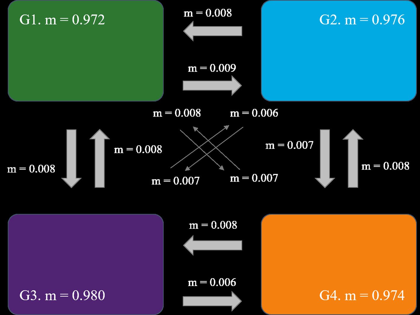
The coefficients of inbreeding obtained using the INEST ranged from 0.0051 in Altamira to 0.2446 in Olmeca (Table 2). Three models were evaluated to detect the presence of recent genetic bottlenecks. The infinite allele model (IAM), the two-phase model (TPM), and the step mutation model (SSM). The SMM model has been suggested as a statistically conservative approach to detect microsatellite bottlenecks (Luikart et al., 1998). However, given the instability and wide range of mutation rates inherent to these markers, the TPM model may be the one that best explains the predominant mutation process at most loci (Di Rienzo et al., 1994). According to the TPM model, 4 populations in O. drummondii show possible recent bottlenecks: Altamira, Ojoshal, Matagorda and La Mancha (Table 2). Regression analyses revealed significant latitudinal clines in genetic diversity, with both alleles per locus (r = 0.69, p < 0.005) and expected heterozygosity (r = 0.65, p < 0.005) showing strong negative relationships with latitude. Latitude significantly predicted the percentage of polymorphic loci (r = 0.4, p < 0.05), whereas no significant relationship was observed for heterozygosity (Supplementary material: Table S5).
Genetic structure
When evaluating the distribution of genetic variation within and among populations, mean values of global inbreeding (FIT = 0.416 ± 0.163) and local inbreeding (FIS = 0.059 ± 0.195) indicated significant heterozygosity deficits. The mean value of genetic differentiation (FST) was 0.376 ± 0.132, indicating that 38% of the genetic variation in O. drummondii was due to differences between populations. Furthermore, genetic differentiation between pairs of populations was mostly high (> 0.15). Matagorda and Bolívar had the lowest differentiation (0.06), followed by Punta Arena del Sur and Agua Blanca (0.17), and Bolívar and South Padre Island (0.18). The analysis of molecular variance (AMOVA) showed that most genetic variation was found among individuals (54%), followed by that found among populations (38%) (Table 3).
The Mantel test detected significant isolation by distance (r = 0.64, p = 0.002). The BAYESASS analysis revealed high diagonal m-values (G1 = 0.972 – G3 = 0.980), suggesting high gene flow within the individual groups. Higher gene flow was observed from G1 to G2 (m1 to 2 = 0.009) (Fig. 2). The results of the Bayesian clustering are shown in Supplementary material: Fig. S1. The most probable K with the highest value of ΔK = 479.023 was K = 3, followed by K = 4 with ΔK = 101.129. For K = 3, 3 clearly defined genetic groups were observed, with a very low proportion of admixture among them. In this case, the first group consisted of the Texas populations: Bolívar, Matagorda, and South Padre Island, and the northernmost Mexican population, Altamira. The second group included the 3 remaining Mexican populations in the Gulf of Mexico: La Mancha, Olmeca and Ojoshal, while the third group comprised the 2 populations on the Baja California Peninsula. For K = 4, the clustering is similar to K = 3. The main difference in this case was that the fourth cluster split the previous cluster containing the Texas and Altamira populations, indicating greater genetic correspondence between Bolívar and Matagorda (populations further north in the Gulf) and between South Padre Island and Altamira. Admixture was low, indicating that Oenothera populations are highly structured.
The Discriminant Analysis of Principal Components (DAPC), like the Bayesian method, also showed 4 groups (Fig. 1C; Supplementary material: Fig. S2). Consistent with the results of Structure, one group was formed by the populations of Baja California (Punta Arena del Sur and Agua Blanca). However, in this case, La Mancha was no longer grouped together with Ojoshal and Olmeca, which formed the second group. Altamira and La Mancha formed a third group that is closer to the fourth formed by the Texan populations (Bolívar, Matagorda, and South Padre Island). The DAPC results indicated the possibility that the Texas group was the ancestral group of the central Gulf of Mexico populations (Altamira and La Mancha). The other 2 groups were markedly more differentiated.
Table 3
Molecular variance analysis (AMOVA) of Oenothera drummondii populations.
| Source of variation | df | Sum sq | Mean sq | Variance component | Total variance (%) | p values |
| Between populations | 8 | 841.68 | 105.21 | 2.78 | 37.39 | 0.001 |
| Among populations | 153 | 807.84 | 5.28 | 0.61 | 8.21 | 0.001 |
| Within individuals | 162 | 657 | 4.05 | 4.05 | 54.39 | 0.001 |
| Total | 323 | 2,306.53 | 7.14 | 7.45 | 100 |
Discussion
In this research, we evaluated the genetic variation between and within populations of Oenothera drummondii throughout its range in North America, for which we used microsatellite markers. These markers demonstrated sufficient variability to resolve population genetic structure at high resolution, consistent with a previous study (Hernández-Espinosa et al., 2020). We also found that all populations were in linkage disequilibrium for at least one locus. Deviations may result from limited homologous recombination during meiosis when chromosomal rings are formed (Rauwolf et al., 2008). In O. drummondii, as in many Oenothera species, this limited recombination is reported to cause changes in the linkage equilibrium (Cleland, 1972; Rauwolf et al., 2008; Raven, 1979), as described in other ring-forming species of the genus: O. biennis (Larson et al., 2008; Levin, 1975; Levy & Levin, 1975), O. harringtonii (Skogen et al., 2012), O. hartwegii and O. gayleana (Lewis et al., 2016). The unique recombination system in the Oenothera is an attribute that has allowed them to colonize new environments from their origin in the Miocene (ca. 20 Ma), until recent times, successfully establishing themselves first in the Neotropics and then in Europe (Dietrich et al., 1997; Wagner et al., 2007).
Compared to other plants with similar characteristics in lifeform, reproductive system, geographic range, and dispersal mechanism, we found that Oenothera drummondii showed moderate to low genetic diversity. This is a short-lived perennial, self-compatible species with a mixed reproductive system and wide distribution (Dietrich & Wagner, 1988), and a variety of dispersal mechanisms (Gallego-Fernández et al., 2021). Mean levels of genetic diversity reported for other plants with mixed reproduction (N = 15, mean HE = 0.60), short-lived perennial life form (N = 29, mean HE = 0.55), wide distribution (N = 31, mean HE = 0.62), and water or wind dispersal (N = 28, mean HE = 0.61) (Nybom & Bartish, 2000), were higher than the level found in O. drummondii (mean HE = 0.442).
Historically, genetic diversity in Oenothera has been attributed to structural genomic rearrangements, particularly hybridization and reciprocal translocations that alter linkage relationships translocations (Cleland, 1972; Rauwolf et al., 2011), as the genomes in Oenothera were considered to be essentially “non-recombining” due to the formation of chromosomal rings during meiosis (Cleland, 1972; Golczyk et al., 2014; Rauwolf et al., 2008). In contrast, the reported genetic diversity in Oenothera species appears strongly influenced by their predominant reproductive system. O. biennis, a permanent translocation heterozygote (PTH), maintains higher genetic variation than O. drummondii, which exhibits a mixed mating system (mean HE = 0.69 vs. 0.44) (Larson et al., 2008). This agreed with the expectation of the “functional” asexual reproductive system of O. biennis, in which autogamy is almost complete and offspring are mostly clonal (Mather, 1943; Stebbins, 1957). Consistent with expectations for obligate sexual reproduction, self-incompatible, bivalent-forming Oenothera species (O. harringtonii with mean HE = 0.77, O. gayleana with mean HE = 0.53 and O. hartwegii with mean HE = 0.49 vs O. drummondii with HE = 0.44) maintained significantly higher genetic diversity than the mixed-mating O. drummondii (HE = 0.44) (Levin, 1975; Rhodes et al., 2014; Skogen et al., 2019).
In terms of its reproductive system, the self-compatible O. drummondii generally has large flowers and an elevated stigma, suggesting a high propensity for sexual reproduction, although it can self-pollinate in the absence of pollinators or in situations where self-fertilization is evolutionarily advantageous (Gregory, 1964; Sicard & Lenhard, 2011). Gallego-Fernández and García-Franco (2021b) assessed the level of self-compatibility of O. drummondii in the Gulf of Mexico, through germination essays. They evaluated 4 of the 9 populations in this study (Bolívar, South Padre Island, La Mancha and Ojoshal), and found that self-compatibility increased in low-latitude populations (La Mancha and Ojoshal), while lower for higher-latitude populations (Bolívar and South Padre Island). These results suggest a latitudinal shift towards greater selfing to the south of the distribution. It has been suggested that greater selfing in populations leads to a decrease in genetic diversity (Ingvarsson, 2002), which is consistent with the pattern of genetic variation found in this study. In agreement with the results of Gallego-Fernández and García-Franco (2021a), we found that populations with higher reported self-compatibility also had lower genetic diversity. On the other hand, in partial selfing species, reductions in genetic diversity are associated with changes in traits that facilitate selfing (i.e., reduced flower size, reduced nectar, pollen and reduced herkogamy) (Barrett & Harder, 1996; Shimizu & Tsuchimatsu, 2015; Tedder et al., 2015). According to the theory, it would be expected that the populations of O. drummondii with a higher self-compatibility, and lower genetic diversity (i.e., Ojoshal) would also show a tendency to reduce flower size, and populations with lower self-compatibility, and higher genetic diversity (i.e., Bolívar) would show an increase in flower size. However, Gallego-Fernández and García-Franco (2021a) found the opposite: populations showed larger flower sizes following a latitudinal gradient from subtropical (i.e., Bolívar and South Padre Island) to tropical (i.e., La Mancha and Ojoshal) climates. This result suggests that in O. drummondii there is no latitudinal correlation between a reduction in flower size and an increase in selfing, and thus to a reduction in genetic diversity. Differences in floral traits among O. drummondii populations appear to respond to both biotic (i.e., pollinators) and abiotic factors (i.e., temperature, precipitation), suggesting local adaptations to environmental changes (Gallego-Fernández & García-Franco, 2021a).
In O. drummondii the genetic diversity showed a significant increase with latitude, with its lowest values in Ojoshal and Olmeca, while the higher values were found in Bolívar and Matagorda, populations in the highest latitudes. The genus Oenothera appears to have originated in northern Mexico and the adjacent USA, and subsection Raimmania, to which O. drummondii belongs, is centered in this area (Dietrich & Wagner, 1988). Since older clades tend to have more genetic diversity (Willi et al., 2018), it would be expected that the greatest genetic diversity would be found in populations at latitudes closest to the center of origin (i.e., Bolívar and Matagorda) and that it would lower as populations moved away to the periphery of the distribution, as was found here. In addition to reducing population genetic variation through genetic drift, habitat suitability often decreases from the core to the edge of a species’ geographic range, leaving edge populations small and isolated (Sagarin & Gaines, 2002), as in Ojoshal. However, despite the small population size of Ojoshal, inbreeding was low, presumably because of its high selfing index (Gallego-Fernández & García-Franco, 2021b). Inbreeding depression is predicted to be lower in selfing species because recessive deleterious alleles are expected to be efficiently “purged” from populations (Winn et al., 2011), and selfing favors the selection of new recessive beneficial mutations (Burgarella & Glémin, 2017; Charlesworth et al., 1993).
The pattern of distribution of the genetic diversity found in Oenothera drummondii seems to be shaped by demographic and evolutionary processes (Durka, 1999; Hewitt, 1996). Historical climate-driven changes are known to still affect the present-day genetic diversity (Alvarez et al., 2009; Hewitt, 2000). As a result of sequential founder events during post-glacial recolonization, contemporary populations show reduced genetic diversity and increased genetic differentiation, especially at range margins (Eckert et al., 2008; Sagarin & Gaines, 2002). The above pattern was found in 512 North American herbs, showing that the shifting and fragmentation of species’ geographical ranges in the past 20,000 years has played an important role in shaping the genetic variation of contemporary populations (Benavides et al., 2019).
Regarding the populations in Baja California (i.e., Agua Blanca and Punta Arena del Sur), the results of both genetic diversity and genetic structure showed that they formed an independent genetic group, as expected given that the populations belong to a different subsp. of O. drummondii. However, based on the genetic differences detected and the evidence of differences in life history, vegetative and floral characteristics observed in the field at the time of collection, it is suggested that O. drummondii subsp. thalassaphila is a distinct species from O. drummondii subsp. drummondii (Table 4). A detailed taxonomic study and additional genetic data from new populations of O. drummondii subsp. thalassaphila will be needed to support this.
Table 4
Distinctive morphological attributes between O.drummondii subsp. drummondii and O. drummondii subsp. thalassaphila. Data taken from Benavides et al. (2019).
| O.drummondii subsp. drummondii | O. drummondii subsp. thalassaphila | |
| Habit | Annual herb | Perennial sudshrub |
| Stem pubescence | Strigillose to villous | Strigillose |
| Glandular puberulent hairs | Present | Absent |
| Cauline leaves | 1-8cm, oblanceolate to obovate, densely villous, margins entire to remotely sinuate dentate | 1-4.5cm, oblong lanceolate to oblanceolate, strigillose, marginis entire to coarsely dentate |
| Floral tube | 2.5-5cm, strigillose to densely villous | 2-3.5cm, strigillose |
| Sepals | 2-3cm, strigillose to villous | 1.3-2.5cm, strigillose, occasionally red doted |
| Petal length | 2.5-4.5cm | 2-3.5cm |
| Capsule | 2.5-5.5cm, strigillose to villous | 2-4cm, strigillose |
| Seeds | 1.1-1.7mm | 1.5-2mm, smooth |
We conclude that the genetic diversity and genetic structure across the range of O. drummondii in North America suggest a latitudinal shift towards increased selfing and a decline in genetic diversity in the low-latitude populations. However, there is no positive relation between reductions in floral traits and increased selfing in the populations. Differences in floral traits appear to respond to biotic and abiotic factors, suggesting local adaptations to environmental changes. In O. drummondii, genetic parameters may reflect historical processes like climate-driven changes (i.e., the last glaciation), and patterns of genetic distribution associated with them, such as the center-peripheral hypotheses. The genetic attributes evaluated here suggest that populations of O. drummondii subsp. thalassaphila may represent a distinct species, but further evaluation will be required to confirm this hypothesis.
Acknowledgments
This study was supported by the Consejo Nacional de Ciencia y Tecnología (Conacyt) by a scholarship (2019-000037-02NACF-29365), as part of a doctoral thesis directed by Jorge González-Astorga. This study was also supported by the Ministerio de Economía y Competitividad, Spain (MINECO Project CGL2015-65058-R co-funded by FEDER). We sincerely thank the assistance in fieldwork to collect plant materials: Rusty Feagin, José García-Franco, Alejandro Espinosa de los Monteros and Anwar Medina-Villareal. We also thank Janet Nolasco-Soto for the assistance in laboratory methods, and two anonymous reviewers for their comments and observations on the manuscript.
References
Alvarez, N., Thiel-Egenter, C., Tribsch, A., Holderegger, R., Manel, S., Schönswetter, P. et al. (2009). History or ecology? Substrate type as a major driver of patial genetic structure in Alpine plants. Ecology Letters, 12, 632–640. https://doi.org/10.1111/j.1461-0248.2009.01312.x
Barrett, S. C. H., & Harder, L. D. (1996). Ecology and evolution of plant mating. Trends in Ecology & Evolution, 11, 73–79. https://doi.org/10.1016/0169-5347(96)81046-9
Benavides, E., Kuethe, J. R., Ortiz-Alcaraz, A., & De La Luz, J. L. L. (2019). Oenothera resicum (Onagraceae), a new species and the first record of the family from the Revillagigedo Archipelago, Mexico. Phytotaxa, 416, 59–66. https://doi.org/10.11646/phytotaxa.416.1.7
Burgarella, C., & Glémin, S. (2017). Population genetics and genome evolution of selfing species. In J. Wiley & Sons (Ed.), Encyclopedia of Life Sciences (pp. 1–8). Hoboken, NJ: Wiley. https://doi.org/https://doi.org/10.1002/9780470015902.a0026804
Castillo-Infante, F. R., Mendoza-González, G., Rioja-Nieto, R., & Gallego-Fernández, J. B. (2021). Range Shifts in the Worldwide expansion of Oenothera drummondii subsp. drummondii, a plant species of coastal dunes. Diversity, 13, 603. https://doi.org/10.3390/d13110603
Cavalli-Sforza, L. L., & Edwards, A. W. F. (1967). Phylogenetic analysis. Models and estimation procedures. American Journal of Human Genetics, 19, 233.
Chapuis, M. P., & Estoup, A. (2007). Microsatellite null alleles and estimation of population differentiation. Molecular Biology and Evolution, 24, 621–631. https://doi.org/10.1093/molbev/msl191
Charlesworth, B., Morgan, M. T., & Charlesworth, D. (1993). The effect of deleterious mutations on neutral molecular variation. Genetics (United States), 134. https://doi.org/10.1093/genetics/134.4.1289
Charlesworth, D. (2006). Evolution of plant breeding systems. Current Biology, 16, R726–R735. https://doi.org/10.1016/j.cub.2006.07.068
Chung, M. Y., Merilä, J., Li, J., Mao, K., López-Pujol, J., Tsumura, Y. et al. (2023). Neutral and adaptive genetic diversity in plants: an overview. Frontiers in Ecology and Evolution, 11, 1116814. https://doi.org/10.3389/fevo.2023.1116814
Chybicki, I. J. (2017). INEST 2.2: the user manual. Poland: Department of Genetics, Kazimierz Wielki University.
Cleland, R. E. (1972). Oenothera, cytogenetics and evolution. London, NY: Academic Press.
Devaux, C., Lepers, C., & Porcher, E. (2014). Constraints imposed by pollinator behaviour on the ecology and evolution of plant mating systems. Journal of Evolutionary Biology, 27, 1413–1430. https://doi.org/10.1111/jeb.12380
Di Rienzo, A., Peterson, A. C., Garza, J. C., Valdes, A. M., Slatkin, M., & Freimer, N. B. (1994). Mutational processes of simple-sequence repeat loci in human populations. Proceedings of the National Academy of Sciences, 91, 3166–3170. https://doi.org/10.1073/pnas.91.8.3166
Dietrich, W., & Wagner, W. L. (1988). Systematics of Oenothera Section Oenothera Subsection Raimannia and Subsection Nutantigemma (Onagraceae). Systematic Botany Monographs, 24, 1–91. https://doi.org/10.2307/25027713
Dietrich, W., Wagner, W. L., & Raven, P. H. (1997). Systematics of Oenothera section Oenothera subsection Oenothera (Onagraceae). Systematic Botany Monographs, 50, 1–234. https://doi.org/10.2307/25027870
Duminil, J., Hardy, O. J., & Petit, R. J. (2009). Plant traits correlated with generation time directly affect inbreeding depression and mating system and indirectly genetic structure. BMC Evolutionary Biology, 9, 177. https://doi.org/10.1186/1471-2148-9-177
Durka, W. (1999). Genetic diversity in peripheral and subcentral populations ofCorrigiola litoralis L.(Illecebraceae). Heredity, 83, 476–484. https://doi.org/10.1038/sj.hdy.6886000
Earl, D. A., & VonHoldt, B. M. (2012). STRUCTURE HARVESTER: a website and program for visualizing STRUCTURE output and implementing the Evanno method. Conservation Genetics Resources, 4, 359–361. https://doi.org/10.1007/s12686-011-9548-7
Eckert, C. G., Samis, K. E., & Lougheed, S. C. (2008). Genetic variation across species’ geographical ranges: the central-marginal hypothesis and beyond. Molecular Ecology, 17, 1170–1188. https://doi.org/10.1111/j.1365-294X.2007.03659.x
Evanno, G., Regnaut, S., & Goudet, J. (2005). Detecting the number of clusters of individuals using the software STRUCTURE: a simulation study. Molecular Ecology, 14, 2611–2620. https://doi.org/10.1111/j.1365-294X.2005.02553.x
Excoffier, L., & Lischer, H. E. L. (2010). Arlequin suite ver 3.5: a new series of programs to perform population genetics analyses under Linux and Windows. Molecular Ecology Resources, 10, 564–567. https://doi.org/10.1111/j.1755-0998.2010.02847.x
Gallego-Fernández, J. B., & García-Franco, J. G. (2021a). Floral traits variation in Oenothera drummondii subsp. drummondii across a wide latitudinal range of native and non-native populations. Flora, 280, 151851. https://doi.org/https://doi.org/10.1016/j.flora.2021.151851
Gallego-Fernández, J. B., & García-Franco, J. G. (2021b). Self-compatibility and reproductive success of Oenothera drummondii subsp. drummondii: is it similar between native and non-native populations? Diversity, 13, 431. https://doi.org/10.3390/d13090431
Gallego-Fernández, J. B., Martínez, M. L., García-Franco, J. G., & Zunzunegui, M. (2021). Multiple seed dispersal modes of an invasive plant species on coastal dunes. Biological Invasions, 23, 111–127. https://doi.org/10.1007/s10530-020-02359-6
Golczyk, H., Massouh, A., & Greiner, S. (2014). Translocations of chromosome end-segments and facultative hetero-
chromatin promote meiotic ring formation in evening primroses. The Plant Cell, 26, 1280–1293. https://doi.org/10.1105/tpc.114.122655
González, D., & Vovides, A. (2002). Low intralineage divergence in Ceratozamia (Zamiaceae) detected with nuclear ribosomal DNA ITS and chloroplast DNA trnL-F non-coding region. Systematic Botany, 27, 654–661. https://doi.org/10.1043/0363-6445-27.4.654
Gregory, D. P. (1964). Hawmoth pollination in the Genus Oenothera. Journal of Systematic and Evolutionary Botany, 5, 385–420.
Greiner, S., & Köhl, K. (2014). Growing evening primroses (Oenothera). Frontiers in Plant Science, 5, 80880. https://doi.org/10.3389/fpls.2014.00038
Hamrick, J., & Godt, M. (1996). Effects of life history traits on genetic diversity in plant species. Philosophical Transactions of the Royal Society of London. Biological Sciences, 351, 1291–1298. https://doi.org/10.1098/rstb.1996.0112
He, Z. Z., Stotz, G. C., Liu, X., Liu, J. J., Wang, Y. G., Yang, J. et al. (2024). A global synthesis of the patterns of genetic diversity in endangered and invasive plants. Biological Conservation, 291, 110473. https://doi.org/https://doi.org/10.1016/j.biocon.2024.110473
Hernández-Espinosa, R., González-Astorga, J., de los Monteros, A. E., Cabrera-Toledo, D., & Gallego-Fernández, J. B. (2020). Transferability of microsatellite markers developed in Oenothera spp. To the invasive species Oenothera drummondii Hook. (Onagraceae). Diversity, 12, 1–13. https://doi.org/10.3390/d12100387
Hewitt, G. (2000). The genetic legacy of the Quaternary ice ages. Nature, 405, 907–913. https://doi.org/10.1038/35016000
Hewitt, G. M. (1996). Some genetic consequences of ice ages, and their role in divergence and speciation. Biological Journal of the Linnean Society, 58, 247–276. https://doi.org/10.1111/j.1095-8312.1996.tb01434.x
Holsinger, K. E. (1991). Mass-action models of plant mating systems: the evolutionary stability of mixed mating systems. The American Naturalist, 138, 606–622. https://doi.org/10.1086/285237
Ingvarsson, P. K. (2002). A metapopulation perspective on genetic diversity and differentiation in partially self-fertilizing plants. Evolution, 56, 2368–2373. https://doi.org/10.1111/j.0014-3820.2002.tb00162.x
Johnson, M. T. J., Agrawal, A. A., Maron, J. L., & Salminen, J. P. (2009). Heritability, covariation and natural selection on 24 traits of common evening primrose (Oenothera biennis) from a field experiment. Journal of Evolutio-
nary Biology, 22, 1296–1307. https://doi.org/10.1111/j.14209101.2009.01747.x
Johnson, M. T. J., Fitzjohn, R. G., Smith, S. D., Rausher, M. D., & Otto, S. P. (2011). Loss of sexual recombination and segregation is associated with increased diversification in evening primroses. Evolution, 65, 2873–2889. https://doi.org/10.1111/j.1558-5646.2011.01378.x
Koelling, V. A., Hamrick, J. L., & Mauricio, R. (2011). Genetic diversity and structure in two species of Leavenworthia with self-incompatible and self-compatible populations. Heredity, 106, 310–318. https://doi.org/10.1038/hdy.2010.59
Kopelman, N. M., Mayzel, J., Jakobsson, M., Rosenberg, N. A., & Mayrose, I. (2015). Clumpak: a program for identifying clustering modes and packaging population structure inferences across K. Molecular Ecology Resources, 15, 1179–1191. https://doi.org/10.1111/1755-0998.12387
Larson, E. L., Bogdanowicz, S. M., Agrawal, A. A., Johnson, M. T. J., & Harrison, R. G. (2008). Isolation and characterization of polymorphic microsatellite loci in common evening primrose (Oenothera biennis). Molecular Ecology Notes, 8, 80–81. https://doi.org/10.1111/j.1471-8286.2007.01983.x
Lawrence, E. R., & Fraser, D. J. (2020). Latitudinal biodiversity gradients at three levels: linking species richness, population richness and genetic diversity. Global Ecology and Biogeography, 29, 770–788. https://doi.org/https://doi.org/10.1111/geb.13075
Levin, D. A. (1975). Genic heterozygosity and protein polymorphism among local populations of Oenothera biennis. Genetics, 79, 477–491. https://doi.org/10.1093/genetics/79.3.477
Levin, D. A. (2012). Mating system shifts on the trailing edge. Annals of Botany, 109, 613–620. https://doi.org/10.1093/aob/mcr159
Levy, M., & Levin, D. A. (1975). Genic heterozygosity and variation in permanent translocation heterozygotes of
the Oenothera biennis complex. Genetics, 79, 493–512. https://doi.org/10.1093/genetics/79.3.493
Lewis, E. M., Fant, J. B., Moore, M. J., Hastings, A. P., Larson, E. L., Agrawal, A. A. et al. (2016). Microsatellites for Oenothera gayleana and O. hartwegii subsp. filifolia (Onagraceae), and their Utility in section Calylophus. Applications in Plant Sciences, 4, 1500107. https://doi.org/10.3732/apps.1500107
Luikart, G., Allendorf, F., Cornuet, J., & Sherwin, W. (1998). Distortion of allele frequency distributions provides a test for recent population bolttlenecks. Heredity, 89, 238–247. https://doi.org/10.1093/jhered/89.3.238
Mantel, N. (1967). The detection of disease clustering and a generalized regression approach. Cancer Research, 27, 209–220.
Moreno-Casasola, P. (1988). Patterns of plant species distribution on coastal dunes along the Gulf of Mexico. Journal of Biogeography, 15, 787–806. https://doi.org/10.2307/2845340
Nybom, H., & Bartish, I. V. (2000). Effects of life history traits and sampling strategies on genetic diversity estimates obtained with RAPD markers in plants. Perspectives in Plant Ecology, Evolution and Systematics, 3, 93–114. https://doi.org/10.1078/1433-8319-00006
Opedal, Ø. H. (2018). Herkogamy, a principal functional trait of plant reproductive biology. International Journal of Plant Sciences, 179, 677–687. https://doi.org/10.1086/700314
Overson, R. P., Johnson, M. G., Bechen, L. L., Kinosian, S. P., Douglas, N. A., Fant, J. B. et al. (2023). A phylogeny of the evening primrose family (Onagraceae) using a target enrichment approach with 303 nuclear loci. BMC Ecology and Evolution, 23, 66. https://doi.org/10.1186/s12862-023-02151-9
Peakall, R., & Smouse, P. E. (2012). GenALEx 6.5: Genetic analysis in Excel. Population genetic software for teaching and research-an update. Bioinformatics, 28, 2537–2539. https://doi.org/10.1093/bioinformatics/bts460
Pelletier, T. A., & Carstens, B. C. (2018). Geographical range size and latitude predict population genetic structure in a global survey. Biology Letters, 14, 20170566. https://doi.org/10.1098/rsbl.2017.0566
Pritchard, J. K., Wen, X., & Falush, D. (2010). Documentation for structure software: Version 2.3. University of Chicago, Chicago.
R Core Team. (2020). R: a language and environment for statistical computing. R Foundation for Statistical Computing. https://www.r-project.org/
Raduski, A. R., Haney, E. B., & Igić, B. (2012). The expression of self-incompatibility in angiosperms is bimodal. Evolution, 66, 1275–1283. https://doi.org/10.1111/j.1558-5646.2011.01505.x
Rauwolf, U., Golczyk, H., Meurer, J., Herrmann, R. G., & Greiner, S. (2008). Molecular marker systems for Oeno-
thera genetics. Genetics, 180, 1289–1306. https://doi.org/10.1534/genetics.108.091249
Rauwolf, U., Greiner, S., Mráek, J., Rauwolf, M., Golczyk, H., Mohler, V. et al. (2011). Uncoupling of sexual reproduction from homologous recombination in homozygous Oenothera species. Heredity, 107, 87–94. https://doi.org/10.1038/hdy.2010.171
Raven, P. H. (1979). A survey of reproductive biology in Onagraceae. New Zealand Journal of Botany, 17, 575–593. https://doi.org/10.1080/0028825X.1979.10432572
Rhodes, M. K., Fant, J. B., & Skogen, K. A. (2014). Local topography shapes fine-scale spatial genetic structure in the Arkansas Valley evening primrose, Oenothera harringtonii (Onagraceae). Heredity, 105, 900–909. https://doi.org/10.5061/dryad
Rosenberg, N. A. (2004). DISTRUCT: a program for the graphical display of population structure. Molecular Ecology Notes, 4, 137–138. https://doi.org/10.1046/j.1471-8286.2003.00566.x
Sagarin, R. D., & Gaines, S. D. (2002). The ‘abundant centre’ distribution: to what extent is it a biogeographical rule? Ecology Letters, 5, 137–147. https://doi.org/https://doi.org/10.1046/j.1461-0248.2002.00297.x
Shimizu, K. K., & Tsuchimatsu, T. (2015). Evolution of selfing: recurrent patterns in molecular adaptation.Annual Review of Ecology, Evolution, and Systematics, 46, 593–622. https://doi.org/10.1146/annurev-ecolsys-112414054249
Sicard, A., & Lenhard, M. (2011). The selfing syndrome: a model for studying the genetic and evolutionary basis of morphological adaptation in plants. Annals of Botany, 107, 1433–1443. https://doi.org/10.1146/annurev-ecolsys-112414-054249
Skogen, K. A., Hilpman, E. T., Todd, S. L., & Fant, J. B. (2012). Microsatellite primers in Oenothera harringtonii (Onagraceae), an annual endemic to the shortgrass prairie of Colorado. American Journal of Botany, 99, e313–e316. https://doi.org/10.3732/ajb.1200003
Skogen, K. A., Overson, R. P., Hilpman, E. T., & Fant, J. B. (2019). Hawkmoth pollination facilitates long-distance pollen dispersal and reduces isolation across a gradient of land-use change 1. Annals of the Missouri Botanical Garden, 104, 495–511. https://doi.org/10.3417/2019475
Sokal, R., & Rohlf, F. (1995). Biometry: the principles and practices of statistics in Biological Research (Third Ed.). New York: Freeman.
Stebbins, G. (1957). Self-fertilization and population variability in plants. The American Naturalist, 41, 337–352. https://doi.org/10.1086/281999
Tedder, A., Carleial, S., Gołębiewska, M., Kappel, C., Shimizu, K. K., & Stift, M. (2015). Evolution of the selfing syndrome in Arabis alpina (Brassicaceae). Plos One, 10, e0126618. https://doi.org/10.1371/journal.pone.0126618
Wagner, W. L., Hoch, P. C., & Raven, P. H. (2007). Revised classification of the Onagraceae. In C. Anderson (Ed.), Systematic Botany Monographs. The American Society of Plant Taxonomists. https://doi.org/10.1007/bf03027161
Whitehead, M. R., Lanfear, R., Mitchell, R. J., & Karron, J. D. (2018). Plant mating systems often vary widely among populations. Frontiers in Ecology and Evolution, 6, 38. https://doi.org/10.3389/fevo.2018.00038
Willi, Y., Fracassetti, M., Zoller, S., & Van Buskirk, J. (2018). Accumulation of Mutational Load at the Edges of a Species Range. Molecular Biology and Evolution, 35, 781–791. https://doi.org/10.1093/molbev/msy003
Wilson, G. A., & Rannala, B. (2003). Bayesian inference of recent migration rates using multilocus genotypes. Genetics, 163, 1177–1191. https://doi.org/10.1093/genetics/163.3.1177
Winn, A. A., Elle, E., Kalisz, S., Cheptou, P. O., Eckert, C. G., Goodwillie, C. et al. (2011). Analysis of inbreeding depression in mixed-mating plants provides evidence for selective interference and stable mixed mating. Evolution, 65, 3339–3359. https://doi.org/10.1111/j.15585646.2011.01462.x
Wright, S. (1969). Evolution and the genetics of populations: Vol. 2. The theory of gene frequencies. Chicago and
London: University of Chicago Press.
Wright, S. (1978). Evolution and the genetics of populations. Variability within and among natural populations. Vol. 4. Chicago, IL.: University of Chicago Press.

Ensambles de polen moderno y fósil en la sierra Occidental de Jalisco; ~ 1,500 años de historia de la vegetación y cambio ambiental
Modern and fossil pollen assemblages in the Sierra Occidental of Jalisco; ~ 1,500 years of history of the vegetation and environmental change
Ana Patricia del Castillo-Batistaa, *, Blanca Lorena Figueroa-Rangela, Socorro Lozano-Garcíab, Ramón Cuevas-Guzmána, Miguel Olvera-Vargasa y Lia Hueso-Vidrioc
a Universidad de Guadalajara, Laboratorio de Paleoecología y Cambio Climático, Departamento de Ecología y Recursos Naturales, Centro Universitario de la Costa Sur, Av. Independencia Nacional Núm. 151, 48900 Autlán de Navarro, Jalisco, México
b Universidad Nacional Autónoma de México, Instituto de Geología, Laboratorio de Paleoecología, Paleoclimatología y Cambio Climático, Departamento de Dinámica Terrestre Superficial, Ciudad Universitaria, Coyoacán, 02376 Ciudad de México, México
c Universidad de Guadalajara, Ingeniería en Recursos Naturales y Agropecuarios, Departamento de Ecología y Recursos Naturales, Centro Universitario de la Costa Sur, Av. Independencia Nacional Núm. 151, 48900 Autlán de Navarro, Jalisco, México
*Autor para correspondencia: ana.delcastillo@academicos.udg.mx (A.P. del Castillo-Batista)
Recibido: 15 agosto 2025; aceptado: 30 octubre 2025
Resumen
La sierra de Cacoma, Jalisco, es una región de alta diversidad florística y endemismo situada en una zona de transición biogeográfica (2,119 m snm), donde convergen elementos templados y tropicales. Analizamos la relación entre la composición taxonómica del polen moderno y fósil, así como los cambios ambientales en un bosque de Pinus–Quercus–Abies de La Cumbre de Guadalupe (Talpa de Allende, Jalisco, México). Se analizaron 22 muestras de polen moderno, 62 de polen fósil y la estructura de la vegetación en 14 parcelas de 500 m2. Aplicamos los índices de asociación palinológica de Davis, la diversidad de Hill y una similitud basada en la distancia cordal. Los últimos ~ 1,580 años muestran un intervalo de mayor similitud (~ 850 y 400 años cal AP) intercalado por episodios de cambio (~ 1,500, 1,000 y 300 años cal AP), congruentes con transiciones climáticas del Holoceno tardío. En el periodo reciente, incendios y deforestación han favorecido la homogeneización de la vegetación. Estos resultados documentan las respuestas de bosques templados a forzamientos climáticos y antrópicos a escala centenaria y resaltan el valor de integrar lluvia de polen moderno, registros fósiles y métricas de diversidad.
Palabras clave: Actividad antrópica; Bosques templados; Holoceno tardío; Lluvia de polen
Abstract
The Sierra de Cacoma, Jalisco is a region of high floristic diversity and endemism located in a biogeographic transition zone (2,119 m asl), where temperate and tropical elements converge. We analyzed the relationship between the taxonomic composition of modern and fossil pollen and environmental changes in a Pinus-Quercus-Abies forest at La Cumbre de Guadalupe (Talpa de Allende, Jalisco, Mexico). We analyzed 22 modern pollen samples, 62 fossil pollen samples, and vegetation structure in 14 plots (500 m² each). We applied Davis palynological association indices, Hill diversity, and a dissimilarity analysis based on chord distance. The past ~ 1,580 years show an interval of greater similarity (~ 850-400 cal yr BP) interspersed with episodes of change (~ 1,500, 1,000, and 300 cal yr BP), consistent with Late Holocene climatic transitions. In the recent period, fires and deforestation have promoted vegetation homogenization. Overall, these results document the response of temperate forests to climatic and anthropogenic forcing at centennial scales and highlight the value of integrating modern pollen rain, fossil records, and diversity metrics to interpret vegetation and environmental history.
Keywords: Anthropogenic activity; Temperate forests; Late Holocene; Pollen rain
Introducción
Las comunidades vegetales actuales incorporan señales del cambio climático acumuladas a múltiples escalas temporales que son evidentes en la distribución, fenología, dinámica demográfica y composición florística, pero su estructura y trayectoria también responden a otros motores de cambio, como el uso de suelo, régimen de incendios, especies invasoras, perturbaciones antrópicas y variabilidad natural (Jackson y Overpeck, 2000). Estos forzamientos configuran patrones contemporáneos, en los que el clima es determinante. En este contexto, el análisis de polen fósil preservado en sedimentos de hondonadas forestales es una herramienta robusta para reconstruir la historia de la vegetación y su ambiente (Calcote, 1995; Figueroa-Rangel et al., 2020). Los registros polínicos documentan cambios en la composición taxonómica a través del tiempo (Figueroa-Rangel et al., 2016) y mediante un enfoque espacio-temporal, la paleoecología permite interpretar la dinámica de los ecosistemas y las respuestas de la vegetación frente a variaciones y perturbaciones ambientales (Trivi de Mandri et al., 2006).
La reconstrucción paleoecológica se basa en el supuesto de que existe una estrecha relación entre las especies de plantas presentes en el bosque y el polen que éste produce (Erdtman, 1943; Faegri e Iversen, 1989). El polen se libera y se dispersa durante la maduración y apertura de los sacos polínicos y es depositado como sedimento en capas del suelo donde se preserva en condiciones ambientales adecuadas (húmedas y anóxicas). Al analizar los conjuntos de polen fósil presentes en estos sedimentos, es posible inferir la composición de la vegetación que existió en el pasado. Así mismo, la lluvia de polen moderno desempeña un papel importante para comprender la representación del polen en las secuencias sedimentarias y calibrar la interpretación basada en estos registros. El análisis de los conjuntos de polen moderno permite establecer la relación entre la abundancia relativa del polen y la presencia de diferentes especies de plantas en la vegetación actual (Rodríguez-Pérez et al., 2025). Lo que contribuye a mejorar la interpretación de los conjuntos de polen fósil y una comprensión más precisa de los cambios de la vegetación a lo largo del tiempo (Lozano-García et al., 2014).
La abundancia de polen en los sedimentos resulta de la interacción de factores biológicos de las especies fuente como la productividad, modo de dispersión y preservación a través del tiempo (Davis, 1984), además de factores ecológicos locales que integran la estructura de la vegetación desde el rodal hasta su entorno inmediato (diámetro y altura de los árboles, área basal, densidad, frecuencia, composición y fenología), modulando el transporte y la deposición del polen (Davies y Fall, 2001; Faegri e Iversen, 1989), y así mismo de las condiciones físicas de los sedimentos del sitio como el tamaño y morfología del sustrato, oxidación y frecuencia de inundación (Davies y Fall, 2001; Faegri y van der Pijl, 1979; Proctor et al., 1996); finalmente, de las características climáticas y la calidad de la identificación palinológica (Escarraga-Paredes et al., 2014). Por lo tanto, el análisis del polen fósil y el estudio de las lluvias de polen moderno son herramientas complementarias que permiten reconstruir la historia de la vegetación y su ambiente, especialmente en regiones donde no se dispone de información sobre la producción y dispersión de polen (Wright, 1967).
Para comprender mejor la dinámica de la vegetación, es necesario abordarla desde una perspectiva espacio-temporal, donde diferentes procesos físicos y biológicos influyen en los patrones observados en cada escala temporal. Las respuestas de la vegetación a corto plazo se pueden interpretar a través de eventos como incendios, huracanes, enfermedades y extracción de madera, mientras que a largo plazo están involucrados los mecanismos de perturbación ambiental y el desarrollo evolutivo (Delcourt et al., 1983). La escala espacial permite comprender cómo los diferentes tipos de vegetación cercanos geográficamente responden de forma diferenciada en eventos de corto o largo plazo, tales como los regímenes de perturbación y fluctuaciones climáticas (Figueroa-Rangel y Olvera-Vargas, 2018). En este sentido, se han realizado diversos estudios con el uso de polen fósil para reconstruir la historia de la vegetación y el clima en el occidente de México, durante el Holoceno tardío (Figueroa-Rangel et al., 2008; Lozano-García et al., 2021). Estos estudios han proporcionado herramientas para evaluar la paleovegetación y los escenarios climáticos en las regiones de alta montaña y en las regiones tropicales. Sin embargo, se ha prestado poca atención a la comprensión de las relaciones cuantitativas entre la lluvia de polen y la vegetación moderna para la interpretación de la historia de la vegetación y el clima con base en datos de polen fósil.
Un área de gran importancia para realizar estudios que combinen registros de polen fósil y moderno es la región de la sierra de Cacoma, ubicada en el occidente de México. Esta región se destaca por su alta diversidad biológica y endemismo de flora y fauna (Conabio, 2010). Se encuentra en una zona de transición biogeográfica con un rango altitudinal de 650 a 2,740 m, con zonas de transición entre tipos de vegetación templada y tropical (INEGI, 2015). Las zonas de mayor elevación comprenden topografías abruptas, con valles y barrancas profundas que forman microclimas que han servido de refugio para varias comunidades de plantas (Amador-Cruz et al., 2024). Por lo tanto, el presente estudio tiene como objetivo evaluar, mediante el análisis de ensambles de polen moderno y su correspondencia con la estructura de la vegetación, si el espectro de polen fósil refleja los patrones de la distribución actual de la vegetación. Para ello, se plantean los siguientes objetivos: 1) caracterizar la composición taxonómica y la representatividad de la lluvia de polen moderno en el bosque de Pinus–Quercus–Abies en la localidad de La Cumbre de Guadalupe en el municipio de Talpa de Allende, Jalisco, identificando los principales taxones y su relación con la vegetación fuente, 2) analizar la correspondencia entre la estructura de la vegetación actual y la señal polínica mediante análisis cuantitativos de la abundancia del polen moderno y 3) comparar la similitud taxonómica entre los ensambles de polen moderno y fósil de los últimos ~ 1,580 años. Este enfoque permitirá fortalecer la interpretación de los registros paleoecológicos en la región y contribuir al conocimiento sobre las relaciones entre la vegetación actual y la señal polínica moderna en los ecosistemas de alta montaña.
Materiales y métodos
El área de estudio se localiza en la sierra de Cacoma al occidente de Jalisco, México, en la localidad denominada La Cumbre de Guadalupe, una región de confluencia entre la cordillera del Eje Neovolcánico Transversal y la sierra Madre del Sur (fig. 1). Corresponde a una elevación de 2,119 m y se extiende hasta el litoral del Pacífico y la costa del occidente de México (INEGI, 2015). Es una zona de gran complejidad geomorfológica y litológica con afloramientos rocosos formados a partir de procesos tectónicos durante el Cretácico (Conabio, 2010). En el área de estudio domina el tipo de roca ígnea extrusiva, donde la unidad geomorfológica comprende laderas de montaña con pendientes de mediana a muy fuertemente inclinadas (Rodríguez-González, 2015). Los tipos de suelo dominantes son Cambisol y Regosol (INEGI, 2015). Presenta un clima templado subhúmedo, con una temperatura media anual de 14.2 °C. La temperatura media del mes más cálido (mayo y junio) es de 16.7 °C, mientras que la temperatura media del mes más frío es 10.8 (enero y febrero), con una precipitación promedio anual de 2,003 mm con lluvias en verano. La precipitación está concentrada entre mayo a septiembre (Estación 14271, Servicio Meteorológico Nacional, Conagua, 2025). Las principales actividades productivas son la agricultura de temporal, con apertura de áreas para el establecimiento de pastizales, la minería y la extracción de madera (Vargas-Rodríguez et al., 2010).
El bosque de Pinus–Quercus–Abies es una asociación vegetal con distribución restringida cerca del límite altitudinal de la vegetación arbórea (Cuevas-Guzmán et al., 2011; del Castillo-Batista et al., 2018). En diversos estudios florísticos de la zona se ha encontrado una alta diversidad florística para numerosas formaciones vegetales de alta montaña, entre ellas el bosque de Pinus con diferentes asociaciones vegetales (Cuevas-Guzmán et al., 2011; Guerrero-Hernández et al., 2014, 2019). Los tipos de bosque de alta montaña son representados principalmente por bosques de coníferas, donde los géneros representativos son Pinus, Abies, Cupressus, Juniperus y algunas latifoliadas como Quercus, Alnus y Arbutus (Perry et al., 1998).
La diversidad florística del área de estudio corresponde a un tipo de vegetación dominado en el estrato arbóreo por Abies jaliscana, A. religiosa, Alnus acuminata, A. jorullensis, Arbutus xalapensis, Carpinus tropicalis, Clethra fragrans, Pinus devoniana, P. douglasiana, P. oocarpa, P. jaliscana, P. herrerae, P. pseudostrobus, Podachaenium eminens, Quercus castanea, Q. calophylla, Q. scytophylla, Q. magnoliifolia, Q. obtusata y Ternstroemia lineata. Se encuentran algunos arbustos dominantes como Archibaccharis serratifolia, Baccharis heterophylla, B. pteronioides, Fuchsia microphylla, Mimosa albida, Monnina ciliolata y Salvia iodantha. El componente herbáceo es diverso, como Amaranthus palmeri, Chenopodium ambrosoides, Iresine diffusa, Antigonon flavescens, Eryngium alternatum, Bidens odorata, B. aurea, Dahlia coccinea, Ageratina choricephala, Fuchsia fulgens, Rumfordia floribunda, Melampodium perfoliatum, Piqueria triflora, Tagetes filifolia, T. lucida, Crotalaria filifolia, C. mollicula, Dalea obreniformis. Por lo que en este estudio nos referimos a este tipo de vegetación como bosque de Pinus–Quercus–Abies (BPQA) por ser los taxones dominantes.
Se realizó un inventario de la vegetación leñosa en 14 parcelas circulares de 500 m2 cada una, siguiendo el protocolo estándar de Olvera-Vargas y Figueroa-Rangel (2023). Cada parcela se ubicó a una distancia mínima de 50 m respecto de las demás. En cada una se registraron datos ambientales y de localización (localidad, coordenadas, elevación, exposición y pendiente) (material suplementario: tabla S1). Para todos los taxones leñosos con diámetros ≥ 2.5 cm arriba de 1.30 m del nivel del suelo (DN). Con estas mediciones se estimaron indicadores estructurales a nivel de parcela, incluyendo densidad (individuos ha-1) y área basal (m2 ha-1). Se recolectaron ejemplares de herbario para confirmar la determinación taxonómica de las especies. La clasificación de familias siguió el sistema Angiosperm Phylogeny Group IV (2016) y la actualización nomenclatural se verificó en la base de datos Tropicos (www.tropicos.org). Este diseño y conjunto de métricas permiten caracterizar de manera comparable la estructura y composición de la vegetación en el área de estudio.
Se recolectaron 22 muestras de polen moderno dentro de las parcelas para evaluar la relación polen-vegetación a escala local (tabla S1). En cada parcela se establecieron subparcelas de 1 m2, dentro de las cuales se obtuvieron muestras de sedimento superficial (suelo y musgo) a una profundidad de 0-5 cm (Hjelle, 1999). Cada muestra se almacenó para su posterior extracción y análisis. Dado que los ambientes de depósito reciben polen de fuentes locales y regionales, el espectro palinológico está condicionado por procesos tafonómicos modulados por el clima y las propiedades del suelo, lo que afecta la relación polen-vegetación observada (Jacobson y Bradshaw, 1981). En este contexto, asumimos que la señal obtenida es representativa del ecosistema fuente a la escala de captura de nuestros sustratos. Si bien superficies extensas como lagos y humedales maximizan el componente regional y facilitan el vínculo con paleorregistros (Markgraf et al., 2002; Ortuño et al., 2011), el muestreo de sedimento superficial aporta la resolución local necesaria para calibrar e interpretar esa señal más integrada en el sitio de estudio.
Con la finalidad de comparar la relación entre el polen moderno y fósil, se extrajo un núcleo de sedimento que abarca los últimos 1,580 años en el BPQA (del Castillo-Batista et al., 2018). El muestreo consistió en la extracción de un núcleo de sedimento de 62 cm de profundidad con un taladro Eijelkamp (“forest hollow”, sensu Calcote 1995, 1998), en un área abierta del bosque a 2,119 m de elevación en la localidad de La Cumbre de Guadalupe (20°10’17.82” N, 104°42’42.32” O) (fig. 1). Se tomaron muestras de sedimento cada 1 cm para su análisis. La cronología se determinó con base en 4 fechados radiocarbono 14C por medio de la técnica AMS (por sus siglas en inglés, accelerator mass spectrometer) en el laboratorio Beta Analytic, Miami, Florida. Para la calibración en años calendáricos fueron utilizados los programas INCAL04.14 y CALIB v.5.02 de Stuiver y Reimer (Stuiver y Reimer, 1993). Para elaborar la cronología se obtuvo un modelo edad-profundidad por interpolación lineal de acuerdo con el método de Bennett (1994), con el apoyo del software Psimpoll (v. 4.25), lo que permitió estimar la tasa de sedimentación promedio de 25 años/cm.
Para la extracción de polen moderno y el polen fósil de las secuencias sedimentarias, se siguió un protocolo estándar de acetólisis Bennett y Willis (2001). Se agregó una pastilla de Lycopodium clavatum L. (Batch 3862) a cada muestra con el fin de estimar la concentración de granos de polen por cm3 (Stockmarr, 1971). Para obtener el tamaño de muestra estadísticamente significativo, se contabilizaron 400 granos de polen por muestra (Maher, 1972). La determinación de polen y esporas se realizó utilizando la colección de referencia palinológica “The Mexican reference collection of Global Pollen Project” (Figueroa-Rangel, 2017), además de claves palinológicas y bibliografía especializada. Para armonizar la resolución taxonómica entre los ensambles de polen fósil y moderno (en los que no siempre es posible asignar el nivel taxonómico de especie) se elaboró una tabla de equivalencias (material suplementario: tabla S2) que vincula cada tipo de polen moderno con sus especies vegetales potencialmente representadas, agrupadas por forma biológica. Los conteos de polen se expresaron como la suma total en porcentaje del polen de árboles, arbustos, herbáceas y esporas de Pteridophyta sensu lato, consideradas en este trabajo como abundancia de polen (Bennett y Willis, 2001). El polen desconocido se contó, pero fue excluido de la suma total de polen en ambos ensambles. El diagrama de polen fósil se elaboró en Psimpoll (v. 4.25) (Bennett, 2005), mientras que, el de polen moderno en el programa Tilia Graph (Grimm, 2020).
La contribución de cada una de las especies encontradas en la vegetación se estimó utilizando el índice de valor de importancia (IVI) para árboles (Matteucci y Colma, 1982; Whittaker, 1967). Este índice es un valor ponderado de la estructura del bosque, se calcula sumando las variables estructurales de la densidad relativa (número de árboles del taxón dividido entre el número total de árboles de todos los taxones), la frecuencia relativa (número de muestras en las que el taxón aparece dividido entre el número total de muestras) y el área basal relativa (área basal total del taxón dividida entre el área basal total de todos los taxones) (Cottam y Curtis, 1956). De esta manera, el IVI proporciona una medida de la importancia relativa de cada especie en el rodal. Así mismo, para el componente arbóreo se estimó la media de diámetro y altura por especie de todas las parcelas muestreadas.
Para describir la distribución de los diámetros y las alturas de las especies arbóreas en las parcelas muestreadas, se estimó la media del diámetro a la altura de 1.30 m (DN) y la altura total por especie. Se utilizaron diagramas de caja y bigote para identificar la mediana, los cuartiles (Q1 y Q3), el rango intercuartílico y la presencia de valores atípicos, proporcionando información sobre la variabilidad y la tendencia central de cada variable. El análisis fue realizado mediante el software estadístico R Project 3.6.1 (Ihaka y Gentleman,1993).
Para analizar la relación entre las especies y las parcelas basados en el método de Olvera-Vargas y Figueroa-Rangel (2023) se realizó un Análisis de Conglomerados. Es una técnica estadística multivariada que tiene como objetivo agrupar elementos o variables para lograr la máxima homogeneidad dentro de cada grupo y la mayor diferencia entre los grupos. Se trata de una clasificación jerárquica aglomerativa (Clarke y Gorley, 2015). Se utilizó la matriz de densidad de las especies, la cual fue transformada con una doble raíz cuadrada para mejorar la ponderación de las especies raras y abundantes. El análisis se realizó utilizando la medida de distancia Bray-Curtis y como método de unión de grupos de los promedios ponderados, con el apoyo del software PRIMER V.7 (Clarke y Gorley, 2015).
Utilizando datos de presencia-ausencia del polen moderno y de la vegetación, se calcularon 3 índices de asociación R (Davis, 1984), el índice de asociación (A), el índice de sobrerrepresentación (O) y el índice de subrepresentación (U). Estos índices permiten determinar si los taxones están presentes de manera simultánea, tanto en el conjunto de polen como en la vegetación (León-Carreño et al., 2019). Se calcularon con las fórmulas que se describen a continuación:
A = B0 / P0 + P1 + B0
O = P0 / P0 + B0
U = P1 / P1 + B0
Donde B0 corresponde al número de parcelas en las que tanto el tipo polínico como el grupo vegetal asociado están presentes, P0 representa el número de parcelas en las que se registra el polen, pero la planta que lo produce no está presente en la vegetación, y P1 es el número de parcelas en las que el tipo de polen está ausente pero el taxón vegetal se encuentra presente en la vegetación. Los valores del índice de asociación varían entre 0 y 1; donde A = 1 indica que el tipo polínico y el taxón vegetal están siempre presentes y si A = 0, alguno de los 2 elementos se encuentra ausente en todos los levantamientos. Posteriormente, los valores de los índices de cada taxón se agruparon en las siguientes categorías: 1) tipo fuertemente asociado “TFA” cuando A > 0.65; 2) tipo asociado “TA”, cuando A varía entre 0.65 y 0.5; 3) tipo débilmente asociado “TDA”, donde A < 0.5 y además O y U son positivos; 4) tipo sobrerrepresentado “TOR”, cuando A < 0.5 y U = 0; 5) tipo subrepresentado “TUR”, con A < 0.5 y O = 0, y 6) tipo no asociado “TNA”, en donde A = 0, además O y U son positivos (Fjordheim et al., 2018).
La diversidad de taxones de los datos de polen moderno y fósil se estimó mediante la diversidad de Hill N0 sumando el número de taxones identificados en cada conjunto (Hill, 1973). Se calcularon los valores de diversidad de Hill N1 para obtener más información sobre las características de diversidad del polen. Esta métrica considera la riqueza de taxones en cada muestra y pondera cada taxón según su abundancia relativa. Asimismo, se seleccionó el número de Hill N2 para representar el número de taxones de polen fósil que son muy abundantes (dominantes) (Figueroa-Rangel et al., 2020). Estos cálculos se realizaron utilizando la librería “vegan” (Oksanen et al., 2010), disponible en el paquete estadístico R-v3.4.3 (R Core Team, 2019).
Con el propósito de comparar la composición taxonómica entre los ensambles de polen fósil con los de polen moderno, se aplicó la función de comparación de análogos múltiples (analog.mult), que calcula índices de distancia o disimilitud entre las muestras de polen fósil con el moderno. Para ello se utilizó la distancia cordal (square chord distance en inglés) mediante la librería “paleoMAS” (Correa-Metrio et al., 2015) disponible en R (R Core Team, 2019).
Resultados
Se registraron 6 familias, 8 géneros y 17 especies en las 14 parcelas analizadas. Las familias con más riqueza de especies fueron Pinaceae y Fagaceae. Los géneros más frecuentes presentes en las parcelas fueron: Pinus–Quercus–Abies. Pinus pseudostrobus fue la especie dominante en el dosel del rodal por su IVI (tabla 1), seguida por Abies jaliscana, Pinus devoniana, Quercus castanea y P. herrerae, todos ellos identificados como elementos importantes de acuerdo con su IVI. Por otro lado, Q. scytophylla, Q. magnoliifolia y P. douglasiana presentan los valores más bajos de IVI.
El análisis de cuartiles de los diámetros normales de las especies arbóreas muestra que la mayoría de los individuos presentan diámetros inferiores a 60 cm (fig. 2a). Se observa una notable dispersión en la mediana de Vachellia farnesiana, lo que indica una alta variabilidad en el diámetro de esta especie. En contraste, Baccharis pteronioides, Monnina ciliolata y Rumfordia floribunda presentan diámetros más bajos y menos dispersos. Además, Pinus devoniana, P. douglasiana y P. pseudostrobus concentran los valores de diámetros más altos entre las especies analizadas. En cuanto a las alturas, la mayoría de las especies registran valores inferiores a los 30 m (fig. 2b). Quercus calophylla se destaca por su variabilidad en la distribución de alturas, mientras que Baccharis pteronioides, Monnina ciliolata y Rumfordia floribunda presentan alturas significativamente menores y con menor dispersión.
La clasificación de las parcelas generó 4 grupos, mismos que se formaron para la clasificación de las especies. Cuando se presenta el resultado a través del dendrograma de sombras, se observó que algunas especies como Pinus pseudostrobus y P. devoniana se encuentran en los 4 grupos de parcelas, pero en general, hay coincidencia de grupos de especies con los grupos de parcelas. Abies religiosa, Rumfordia floribunda, Monnina ciliolata y Arbutus xalapensis presentaron sus mayores abundancias en la parcela P10 y P11, mientras que Quercus herrerae, Q. magnolifolia y Q. castanea tienen su mayor expresión en abundancias en las parcelas P01, P02, P07 y P08 (fig. 3).
En el espectro polínico del bosque se identificaron 41 taxones, pertenecientes a 31 familias y 40 géneros, que incluyen árboles, arbustos, herbáceas y helechos (material suplementario: tabla S3). Pinus se registró como el taxón dominante en el estrato arbóreo, con más de 60% del espectro polínico. De manera similar, los taxones de Quercus (< 20%) y Abies (< 15%) se encontraron en todo el espectro polínico con porcentajes considerables. En el estrato herbáceo, Poaceae se registró como la más abundante, se encontró en todas las muestras con un porcentaje superior a 5%. Los taxones de Eupatorium (> 5%) y Baccharis (> 5%) se registraron con porcentajes bajos en el componente herbáceo. Polypodiaceae prevaleció con un porcentaje mayor a 5%. No obstante, el grupo de los helechos no alcanzó una representación importante en el espectro polínico (fig. 4).
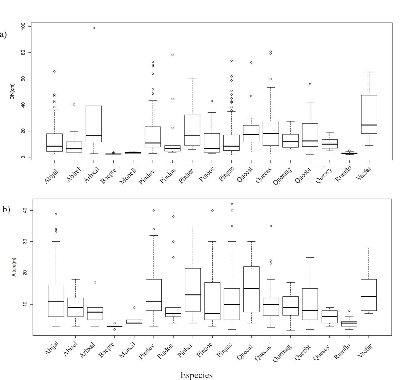
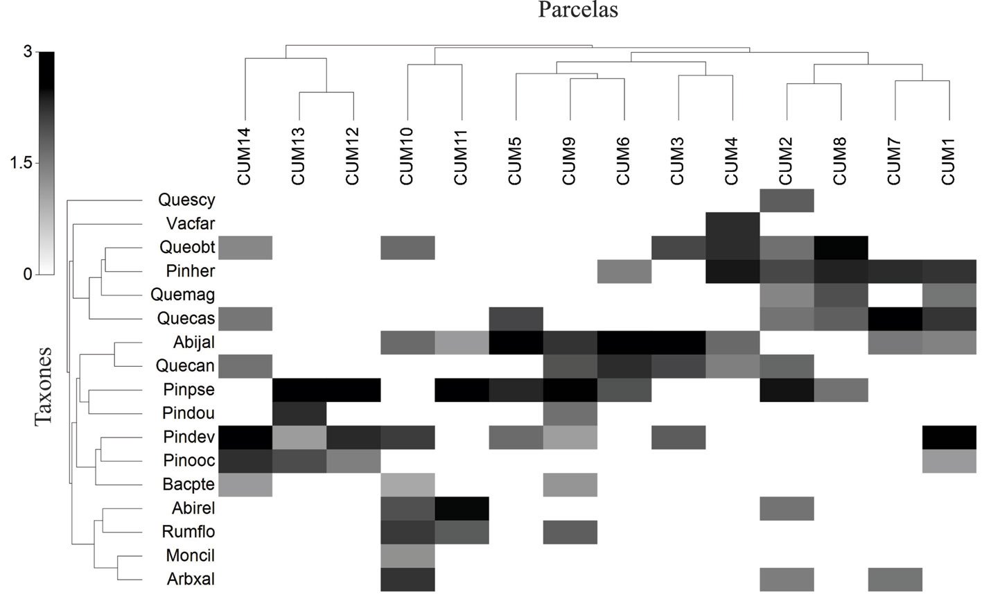
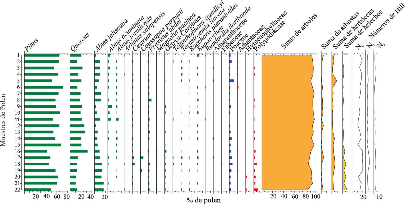
El índice de Davis revela que la mayoría de los taxones polínicos se adscriben al grupo de tipo asociado (TOR); los taxones de polen de Pinus, Quercus, Abies, Arbutus xalapensis, Baccharis pteronioides y Rumfordia floribunda, pertenecen al grupo de tipo asociado (TA), mientras que Monnina ciliolata es el único que se encuentra en el tipo subrepresentado (TUR). Ningún taxón demostró ser fuertemente asociado (TFA) (tabla 2).
Tabla 1
Valores relativos para densidad (Dr), área basal (ABr) y frecuencia (Fr) en árboles del BPQA. Índice de valor de importancia (IVI) para árboles y arbustos.
| Familias | Especies | Dr (%) | ABr (%) | Fr (%) | IVI (%) |
| Asteraceae | Baccharis pteronioides (Bacpte) | 1.02 | 0.02 | 4.23 | 1.86 |
| Rumfordia floribunda (Rumflo) | 15.90 | 0.39 | 4.23 | 6.84 | |
| Ericaceae | Arbutus xalapensis (Axal) | 0.76 | 4.12 | 4.05 | 8.94 |
| Fabaceae | Vachellia farnesiana (Vacfar) | 0.76 | 2.80 | 1.41 | 1.66 |
| Fagaceae | Quercus calophylla (Quecal) | 1.53 | 3.48 | 5.63 | 3.54 |
| Quercus castanea (Quecas) | 5.98 | 12.84 | 9.72 | 9.51 | |
| Quercus magnoliifolia (Quemag) | 1.91 | 1.10 | 4.23 | 2.41 | |
| Quercus obtusata (Queobt) | 5.60 | 6.65 | 8.45 | 6.9 | |
| Quercus scytophylla (Quescy) | 0.89 | 0.34 | 1.41 | 0.87 | |
| Pinaceae | Abies jaliscana (Abijal) | 14.89 | 12.97 | 12.16 | 13.33 |
| Abies religiosa (Abirel) | 7.38 | 2.13 | 4.23 | 4.58 | |
| Pinus devoniana (Pindev) | 9.29 | 14.61 | 11.27 | 11.72 | |
| Pinus douglasiana (Pindou) | 1.65 | 3.08 | 2.82 | 2.51 | |
| Pinus herrerae (Pinher) | 5.47 | 11.45 | 8.45 | 8.46 | |
| Pinus oocarpa (Pinooc) | 4.20 | 2.80 | 5.63 | 4.21 | |
| Pinus pseudostrobus (Pinpse) | 22.14 | 21.19 | 11.27 | 19.19 | |
| Polygalaceae | Monnina ciliolata (Moncil) | 0.64 | 0.02 | 1.41 | 0.69 |
El diagrama polínico del bosque fue dividido en 3 zonas palinológicas mediante un análisis de conglomerados (CONISS) (fig. 5). A lo largo de toda la secuencia del ensamble de polen fósil, se observó un patrón heterogéneo caracterizado por la oscilación de los taxones leñosos herbáceos y helechos. La primera zona palinológica (C-1) corresponde al periodo de 1,580-1,550 años cal AP y muestra una mayor abundancia de taxones leñosos como Alnus, Pinus y Quercus. En cuanto a los taxones herbáceos, los más abundantes fueron Asteraceae, Cyperaceae y Poaceae. La segunda zona (C-2) corresponde al periodo de 1,550-740 años cal AP, abarca el periodo más extenso, presenta un patrón similar al anterior, con la adición de taxones de Fabaceae y Rosaceae. La tercera zona (C-3a) corresponde al año 740-700 años cal AP, se observa un patrón divergente caracterizado por una disminución de Aspleniaceae y Bromeliaceae. En los últimos 700-100 años cal AP (zona C-3b) se aprecia un patrón heterogéneo con oscilaciones en los porcentajes de Pinus, Quercus y Alnus en el grupo de los taxones leñosos, así como en los de Asteraceae, Cyperaceae y Poaceae en el grupo de las herbáceas. En contraste, las esporas como Hymenophyllaceae, Polypodiaceae y Sphagnum disminuyen considerablemente sus porcentajes (fig. 5).
La diversidad de Hill para los conjuntos de polen moderno para el orden N0, indicó que la riqueza es de aproximadamente 16 taxones (con un intervalo de confianza de 95%). Para el orden N1 y N2 obtuvo valores de 3.79-4.76 y 2.4-2.9, respectivamente. Para el conjunto de polen fósil, N0 indicó que la riqueza es de alrededor de 34 taxones (con un intervalo de confianza de 95%), mientras que para N1 y N2 fueron de 14.4-15.8 y 9.4-10.5, respectivamente (figs. 4, 5).
La comparación entre los ensambles de polen moderno y la secuencia de polen fósil de La Cumbre de Guadalupe (fig. 6) mostró distancias cordales al cuadrado que variaron aproximadamente de 0.30 a 0.72. A lo largo de la cronosecuencia predominaron valores intermedios (≈ 0.45-0.60). Se identificaron mínimos locales de disimilitud (˂ 0.40) en intervalos temporales estrechos, destacando un pulso centrado alrededor de ~ 850 años cal AP. En contraste, se observaron franjas con mayor disimilitud (≥ 0.65) especialmente después de ~ 1,000 años cal AP y hacia los extremos de la secuencia. El mejor análogo moderno por nivel fósil rara vez presentó distancias ≤ 0.35 y no se registraron valores cercanos a 0; por lo tanto, no se detectaron análogos modernos muy cercanos para los niveles analizados.
Discusión
El análisis de la vegetación actual en la sierra de Cacoma, Jalisco, muestra que la composición florística está dominada por especies de Pinus–Quercus-Abies como los elementos estructurales más importantes según el IVI. Estos resultados coinciden con estudios previos que han identificado a estos taxones como dominantes en los bosques templados del occidente de México (Cuevas-Guzmán et al., 2011; Guerrero-Hernández et al., 2014, 2019). La estructura diamétrica de la comunidad sugiere una comunidad vegetal joven, con la mayoría de los individuos de diámetros menores de 60 cm, lo que coincide con patrones observados en otras regiones montañosas donde la explotación selectiva ha modificado la distribución diamétrica de las especies arbóreas (Guerrero-Hernández et al., 2022).
Tabla 2
Índice de Davis. La columna de taxones muestra el nombre científico de las especies. (A) significa la asociación, (O) sobrerrepresentación y (U) subrepresentación de los taxones registrados en los ensambles polínicos, basados en datos de presencia/ausencia, tanto de lluvia de polen como de la vegetación del BPQA. Los índices de asociación se clasificaron en: TFA = tipos fuertemente asociados, TA = tipos asociados, TDA = tipos débilmente asociados, TOR = tipos sobrerrepresentados, TUR = tipos subrepresentados y TNA = tipos no asociados.
| Taxones | A | O | U | Tipo |
| Pinus | 0.50 | 0.33 | 0.33 | TA |
| Quercus | 0.50 | 0.33 | 0.33 | TA |
| Abies | 0.50 | 0.35 | 0.32 | TA |
| Alnus acuminata | 0.50 | 0.50 | 0.00 | TOR |
| Alnus jorullensis | 0.50 | 0.50 | 0.00 | TOR |
| Arbutus xalapensis | 0.50 | 0.40 | 0.25 | TA |
| Cestrum | 0.50 | 0.50 | 0.00 | TOR |
| Cornus disciflora | 0.50 | 0.50 | 0.00 | TOR |
| Eugenia | 0.50 | 0.50 | 0.00 | TOR |
| Ficus | 0.50 | 0.50 | 0.00 | TOR |
| Fraxinus uhdei | 0.50 | 0.50 | 0.00 | TOR |
| Juglans major | 0.50 | 0.50 | 0.00 | TOR |
| Magnolia pacifica | 0.50 | 0.50 | 0.00 | TOR |
| Ostrya-carpinus | 0.50 | 0.50 | 0.00 | TOR |
| Ternstroemia lineata | 0.50 | 0.50 | 0.00 | TOR |
| Tilia mexicana | 0.50 | 0.50 | 0.00 | TOR |
| Zinowiewia concinna | 0.00 | 0.00 | 0.00 | – |
| Cupressaceae | 0.00 | 0.00 | 0.00 | – |
| Vachellia farnesiana | 0.50 | 0.50 | 0.00 | TOR |
| Baccharis pteronioides | 0.50 | 0.38 | 0.27 | TA |
| Rumfordia floribunda | 0.50 | 0.25 | 0.40 | TA |
| Monnina ciliolata | 0.50 | 0.00 | 0.50 | TUR |
El análisis del dendrograma de sombras identificó 4 grupos de especies y 4 de parcelas, evidenciando patrones de distribución diferenciados dentro del paisaje forestal. La estructura de los grupos sugiere coexistencia mediada por diferencias fisiológicas y ambientales. El género Pinus domina en la mayoría de los conjuntos en congruencia con su especialización en hábitats de fertilidad baja a moderada y en condiciones abiertas impuestas por aridez, frío o disturbio, así como con historias evolutivas asociadas con altas frecuencias de perturbación, en particular el fuego (Keeley y Zedler, 1998). En contraste, Quercus y Abies conforman subgrupos bien definidos que reflejan preferencias por microambientes más fríos y húmedos (Cuevas-Guzmán et al., 2011; Guerrero-Hernández et al., 2022). La alta similitud florística entre algunas parcelas sugiere que existen factores ambientales y de manejo forestal que han promovido la homogeneización de la vegetación en ciertas áreas, fenómeno que ha sido documentado en otros estudios de dinámica de bosques templados mexicanos (Guerrero-Hernández et al., 2019).
La composición del ensamble polínico moderno refleja la estructura y composición del bosque montano dominado por Pinus–Quercus–Abies. La alta representación de Pinus en el espectro polínico (> 60%) es consistente con estudios previos que han demostrado su alta producción polínica y dispersión anemófila en ecosistemas templados (Castro-López et al., 2020), y coinciden con estudios de lluvia polínica en bosques del occidente y centro de México (Figueroa-Rangel et al., 2016; Lozano-García et al., 2014), los cuales reportan estos elementos con porcentajes superiores a 40% en Pinus y Quercus, mientras que Abies oscila entre 10 y 20%. Estos resultados se explican por los mecanismos de dispersión anemófila y por la gran cantidad de granos de polen que producen (Faegri e Iversen, 1989). La presencia de Quercus y Abies con valores inferiores a Pinus, pero aún representativos (< 20% y < 15%, respectivamente), coincide con su menor producción polínica y las características de dispersión de estos géneros, factores que afectan su representatividad en los registros polínicos modernos (Rodríguez-Pérez et al., 2025).
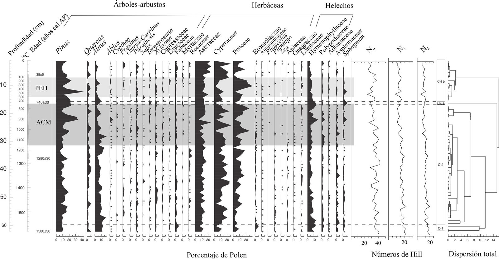
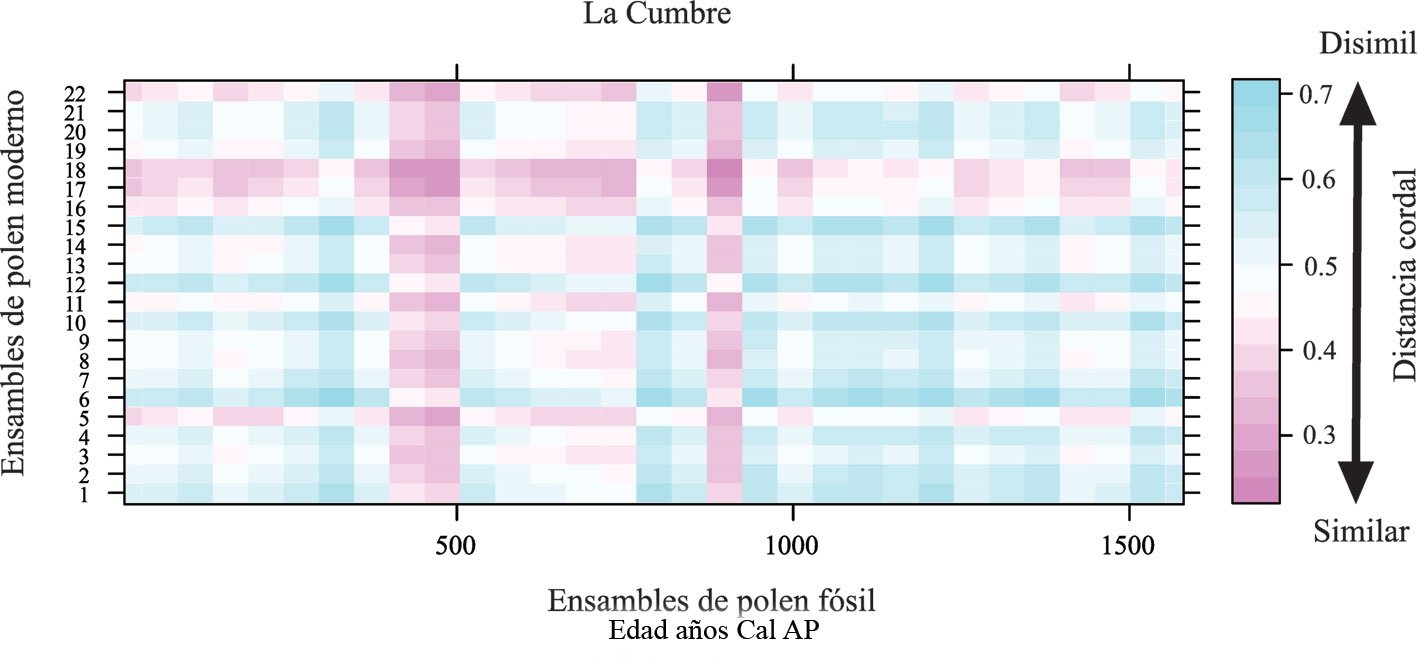
En cuanto a la vegetación herbácea, el predominio de Poaceae (> 5%) indica su importancia en los espacios abiertos del bosque y su alta eficiencia en la producción y dispersión del polen (Hjelle, 1998). La baja representación de Eupatorium y Baccharis (< 5%) sugiere que estas especies, aunque presentes en la vegetación actual, tienen una menor contribución al espectro polínico debido a sus estrategias reproductivas y mecanismos de dispersión, como la entomofilia (Faegri e Iversen, 1989). De manera similar, las esporas de Polypodiaceae, aunque registradas con valores > 5%, no alcanzaron una representación dominante en el espectro polínico, lo que puede atribuirse a que a medida que aumenta la altitud, la representación del polen de la vegetación herbácea disminuye (Markgraf, 1980).
El análisis de representación polínica a través del índice de Davis confirma que los taxones dominantes en el bosque se encuentran principalmente en el grupo de tipo asociado (TA), lo que sugiere una correspondencia adecuada entre la vegetación y el espectro polínico. El predominio del grupo sobrerrepresentado (TOR) para la mayoría de los taxones indica que ciertos elementos del bosque reproducen y dispersan polen en proporciones superiores a su biomasa real en el ecosistema (Jackson y Overpek, 2000). Monnina ciliolata, identificado como tipo subrepresentado (TUR), refleja una producción polínica baja por sus mecanismos de dispersión especializados, lo que puede dificultar su identificación en registros fósiles (Faegri, 1966). La ausencia de taxones en el grupo fuertemente asociado (TFA) sugiere que ningún elemento arbóreo o herbáceo presenta una correspondencia entre su presencia en el bosque y su representación polínica. Este patrón puede explicarse por síndromes de polinización especializados, bajas abundancias locales (León-Carreño et al., 2019) una estructura poblacional dominada por individuos juveniles con pocos adultos reproductivos, como sugiere la distribución de diámetros y alturas (fig. 2).
El ensamble polínico fósil refleja la dinámica de la vegetación durante los últimos ~ 1,580 años, que evidencia cambios en la composición florística asociados a variaciones climáticas y potenciales impactos antrópicos. El diagrama polínico muestra 3 zonas diferenciadas, que sugiere una transición en la estructura del bosque, desde una composición dominada por taxones leñosos hasta un escenario más heterogéneo en los últimos siglos. En la primera zona palinológica (C-1), la dominancia de Alnus, Pinus y Quercus sugiere la prevalencia de un bosque templado de montaña con condiciones húmedas, lo que concuerda con estudios previos en la región del occidente de México (Figueroa-Rangel et al., 2016, 2020). La alta representación de Asteraceae, Cyperaceae y Poaceae indica la presencia de claros en el dosel forestal y espacios abiertos con vegetación herbácea.
Durante la segunda fase, que abarca el periodo más extenso (zona C-2), se mantiene la estructura del bosque, pero con la incorporación de taxones como Fabaceae y Rosaceae, lo que podría indicar una diversificación de la vegetación secundaria y la posibilidad de fluctuaciones climáticas que favorecieron la heterogeneidad del ecosistema (Arellano, 2024). La estabilidad relativa de los elementos leñosos indica que, bajo condiciones climáticas favorables que sostienen la cobertura forestal, el bosque mantiene su estructura y composición con cambios mínimos, evidenciando una alta capacidad de persistencia frente a posibles perturbaciones de baja a moderada intensidad.
El cambio más significativo ocurre en la tercera zona (C-3a), donde se observa una disminución de Aspleniaceae y Bromeliaceae, lo que podría estar vinculado a un enfriamiento o a una reducción en la humedad ambiental, en concordancia con el evento de la Pequeña Edad de Hielo documentado en bosques de alta montaña del occidente de México (Figueroa-Rangel et al., 2019, 2020). Posteriormente, en los últimos 700 años (zona C-3b), la heterogeneidad en las oscilaciones de Pinus, Quercus y Abies sugiere periodos de regeneración y disturbio en el bosque, posiblemente por influencia de actividad humana (del Castillo et al., 2018). La disminución de Cyperaceae, Hymenophyllaceae, Polypodiaceae y Sphagnum podría estar relacionada con una menor disponibilidad de ambientes húmedos o la alteración de los suelos debido a disturbios naturales o inducidos.
El análisis polínico moderno confirma la composición arbórea identificada en campo, con la dominancia de Pinus, Quercus y Abies. Sin embargo, la diversidad de Hill indica una riqueza relativamente baja en el polen moderno (N0 = 16, fig. 4) en comparación con el registro fósil (N0 = 34, fig. 5), lo que sugiere una composición más diversa de la vegetación en el pasado. Esta diferencia podría atribuirse a la dispersión diferencial del polen, a sesgos tafonómicos en la preservación en el sedimento y a la representatividad desigual de ciertos taxones en el espectro polínico (Birks et al., 2011; Xiao et al., 2016). Estudios similares han reportado una disminución de la diversidad arbórea en el Holoceno tardío en otras zonas templadas y tropicales de México, vinculada a eventos de cambio climático y actividades antrópicas (Lozano-García et al., 2021; Ortega-Rosas et al., 2008).
El análisis de los ensambles polínicos modernos y fósiles revela patrones temporales de similitud y disimilitud que sugieren cambios en la composición y estructura de la vegetación a lo largo de los últimos ~ 1,580 años. La mayor similitud entre los registros modernos y fósiles se presenta entre ~ 850 y 400 años cal AP, lo que es congruente con lo reportado en la sierra de Manantlán alrededor de ~ 850 años cal AP, caracterizado por la disminución de Pinus y el aumento de Quercus y Alnus, lo que pareciera una contracción del bosque dominado por Pinus y la expansión relativa de latifoliadas (Figueroa-Rangel et al., 2016). Este intervalo coincide con la Anomalía Climática Medieval (ACM) (800-1200 d.C.), caracterizada regionalmente por condiciones más cálidas y en diversos registros, mayor aridez estacional congruentes con otras secuencias polínicas del occidente y centro de México (Lachniet et al., 2012; Metcalfe et al., 2010), donde Quercus y Alnus se han propuesto como taxones indicadores de sequía (Lozano-García et al., 2021).
La similitud observada hacia ~ 400 años cal AP se acompaña de una expansión relativa de Poaceae y Asteraceae, familias típicamente pioneras y asociadas a ambientes abiertos o recientemente perturbados. Este intervalo coincide con la Pequeña Edad de Hielo (LIA) (1300 y 1850 d.C.), un periodo más frío que el actual que pudo reducir la productividad del bosque, favoreciendo claros y paisajes abiertos propicios para el establecimiento de pastizales (Bradley y Jones, 1993; Mann et al., 2009). Adicionalmente, las perturbaciones antrópicas de los últimos siglos (cambios de uso de suelo, tala y fuego) posiblemente reforzaron esa apertura del paisaje, lo que incrementó la representación polínica de Poaceae y Asteraceae (Lozano-García et al., 2021).
Por otro lado, los periodos de mayor disimilitud identificados hace ~ 1,500, 1,000 y 300 años cal AP, sugieren episodios de cambio ambiental y posibles alteraciones en la vegetación local. Estos periodos de disimilitud se relacionan estrechamente con las 3 zonas identificadas previamente mediante CONISS. La disimilitud hace ~ 1,500 años cal AP coincide con la transición entre las zonas más antiguas de la secuencia, caracterizada por una menor representación de Pinus y un mayor aporte de taxones leñosos y herbáceos indicativos de condiciones más húmedas, lo que significa mayor heterogeneidad ambiental y cambios en la dinámica del bosque (Lachniet et al., 2012). Asimismo, la disimilitud hace ~ 1,000 años cal AP se asocia con un incremento de Abies y una reducción de taxones de ambientes abiertos, lo cual lleva a una reorganización en la composición del bosque, posiblemente asociada a variaciones climáticas durante la Anomalía Climática Medieval; estos episodios han sido relacionados con fluctuaciones de humedad y temperatura que afectaron la distribución de especies arbóreas (Figueroa-Rangel et al., 2016; Metcalfe et al., 2010). En el intervalo más reciente, aproximadamente los últimos 300 años cal AP, se observa un aumento de la disimilitud que marca la transición hacia una señal polínica moderna claramente diferenciada de los ensambles fósiles. Esta modificación puede estar asociada, por un lado, con la variabilidad climática vinculada a la Pequeña Edad de Hielo y por otro lado, con cambios de origen antropogénico posteriores a la colonización española, que implicaron modificaciones del uso del suelo y una mayor presión sobre los ecosistemas como los incendios y procesos de deforestación, que alteraron la estructura y composición del bosque y generaron ensambles polínicos distintos respecto de las condiciones previas (Lozano-García et al., 2021). Estos hallazgos resaltan la interconexión entre los procesos ecológicos y climáticos en la configuración de los ecosistemas forestales, y proporcionan evidencia sobre la sensibilidad de estos ecosistemas a los cambios ambientales pasados.
El análisis de los ensambles polínicos modernos y fósiles en la sierra de Cacoma, Jalisco en particular en la Cumbre de Guadalupe, ha permitido reconstruir la dinámica de la vegetación durante los últimos ~ 1,580 años, que evidencian cambios en la composición y estructura del bosque en respuesta a factores climáticos y antrópicos. Los resultados mostraron que la vegetación actual está dominada por Pinus pseudostrobus y Abies jaliscana, los elementos estructurales más relevantes. Esta composición coincide con la representación polínica moderna, donde Pinus–Quercus–Abies fueron los taxones dominantes, lo que refleja la relación entre el ensamble polínico y la estructura del bosque. Sin embargo, el registro polínico fósil indica que la vegetación del pasado presentaba una mayor diversidad de especies, lo que sugiere una mayor heterogeneidad de la vegetación en el pasado. La disminución de la diversidad efectiva en los últimos siglos podría estar relacionada con el impacto de eventos climáticos, como la Pequeña Edad de Hielo (~ 850-400 AP), así como la influencia de actividades antrópicas, como el cambio en el uso de suelo, los incendios y la explotación forestal.
El análisis de disimilitud entre ensambles de polen moderno y fósil identificó intervalos de mayor similitud estructural del bosque (~ 850 y 400 cal AP), intercalados con episodios de cambio (~ 1,500, ~ 1,000 y ~ 300 cal AP). Estos periodos coinciden con transiciones climáticas del Holoceno tardío, incluida la Anomalía Climática Medieval y la Pequeña Edad de Hielo, que modularon la composición de las comunidades vegetales. Asimismo, la evidencia indica que en los últimos siglos, la actividad humana (incendios, deforestación) ha alterado la estructura forestal y ha favorecido la homogeneización de la vegetación en algunas zonas.
Los hallazgos señalan la relevancia del análisis palinológico en la reconstrucción de la historia ambiental y ecológica de los bosques montanos del occidente de México. Futuros estudios podrían integrar un análisis multiproxy, como datos isotópicos y modelado climático, para mejorar la resolución temporal de los cambios en la vegetación y su relación con la variabilidad climática. Asimismo, se podrían desarrollar análisis de correspondencia entre los conjuntos de polen moderno y la vegetación actual para identificar los factores que explican la ausencia de ciertos taxones esperados, a pesar de la evidencia que indica una correspondencia entre la composición de polen local y la vegetación del bosque.
Agradecimientos
Agradecemos el apoyo financiero de los proyectos Conahcyt CB-2008-106435 y UDG-PTC-1403. Asimismo,
agradecemos al Laboratorio de Paleoecología y Cambio Climático del Departamento de Ecología y Recursos Naturales del Centro Universitario de la Costa Sur, Universidad de Guadalajara, y al Laboratorio de Paleoecología, Paleoclimatología y Cambio Climático del Departamento de Dinámica Superficial del Instituto de Geología, UNAM, por las facilidades, el apoyo logístico y la infraestructura brindados para el desarrollo del estudio. El acceso a la zona de estudio fue brindado por los habitantes de la comunidad de la Cumbre de Guadalupe. También expresamos nuestro reconocimiento a quienes colaboraron en el trabajo de campo, así como a Carlos Armando Pacheco Contreras por la elaboración del mapa y el trabajo de campo. Finalmente, agradecemos a los revisores anónimos por sus observaciones y sugerencias que contribuyeron a mejorar este trabajo.
Referencias
Amador-Cruz, F., Figueroa-Rangel, B. L., Olvera-Vargas, M. y Mendoza, M. E. (2024). A methodological procedure for the estimation of ecological value applied to a neotropical cloud forest. Ecological Research, 40, 437–451. https://doi.org/10.1111/1440-1703.12538
Angiosperm Phylogeny Group IV. (2016). An update of the Angiosperm Phylogeny Group classification for the orders and families of flowering plants: APG IV. Botanical Journal of the Linnean Society, 181, 1–20. https://doi.org/10.1111/boj.12385
Arellano, V. (2024). Vegetation dynamics and climate change resilience in tropical rainforests in Mexico. American Journal of Climatic Studies, 1, 43–55.
Bennett, K. D. (1994). Confidence intervals for age estimates and deposition times in late-quaternary sediment sequences. The Holocene, 4, 337–348. https://doi.org/10.1177/095968369400400401
Bennett, K. D. y Willis, K. J. (2001). Pollen. En J. P. Smol, H. J. B. Birks y W. M. Last (Eds.), Tracking environmental change using lake sediments: volume 3 Terrestrial, algal, and siliceous indicators (pp. 5–32). Amsterdam: Kluwer Academic Publishers. https://doi.org/10.1007/s00334-006-0066-6
Bennett, K. D. (2005). PSIMPOLL 4.25 and PSCOMB 1.03: C Programs for plotting pollen diagrams and analysing pollen data. Uppsala Universitet, Uppsala, Sweden.
Birks, H. J. B., Heiri, O., Seppä, H. y Bjune, A. E. (2011). Strengths and weaknesses of quantitative climate reconstructions based on late-Quaternary biological proxies. Open Ecology Journal, 3, 68–110. https://doi.org/10.2174/1874213001003020068
Bradley, R. S. y Jones, P. D. (1993). ‘Little Ice Age’ summer temperature variations: their nature and relevance to recent global warming trends. The Holocene, 3, 367–376. https://doi.org/10.1177/095968369300300409
Calcote, R. (1995). Pollen source area and pollen productivity: evidence from forest hollows. Journal of Ecology, 83, 591–602. https://doi.org/10.2307/2261627
Calcote, R. (1998). Identifying forest stand types using pollen from forest hollows. The Holocene, 8, 423–432. https://doi.org/10.1191/095968398670894847
Castro-López, V., Domínguez-Vázquez, G., Islebe, G. A., Priego-Santander, Á. G. y Velázquez, A. (2020). Modern pollen-vegetation relationships across a landscape mosaic in central México. Review of Palaeobotany and Palynology, 289, 104362. https://doi.org/10.1016/j.revpalbo.2020.10436
Clarke, K. R. y Gorley, R. N. (2015). Primer v7: Use manual tutorial. Reino Unido Plymouth: PRIMER-E.
Conabio (Comisión Nacional para el Conocimiento y Uso de la Biodiversidad). (2010). El bosque mesófilo de montaña en México: amenazas y oportunidades para su conservación y manejo sostenible. México D.F.: Comisión Nacional para el Conocimiento y Uso de la Biodiversidad.
Conagua (Comisión Nacional del Agua). (2025). Normales climatológicas por estado. Sistema Meteorológico Nacional. Recuperado el 02 octubre, 2025 de: https://smn.conagua.gob.mx/es/climatologia/informacion-climatologica/normales-climatologicas-por-estado
Correa-Metrio, A., Urrego, D. H., Cabrera, K. R. y Bush, M. B. (2015). paleoMAS: Paleoecological Analysis. The R PRoject for Statistical Computing. http://CRAN.R-project.org/package=paleoMAS.
Cottam, G. y Curtis, J. T. (1956). The use of distance measures in phytosociological sampling. Ecology, 37, 451–460. https://doi.org/10.2307/1930167
Cuevas-Guzmán, R., Cisneros-Lepe, E. A., Jardel-Peláez, E. J., Sánchez-Rodríguez, E. V., Guzmán-Hernández, L., Núñez-López, N. M. et al. (2011). Análisis estructural y de diversidad en los bosques de Abies de Jalisco, México. Revista Mexicana de Biodiversidad, 82, 1219–1233. https://doi.org/10.22201/ib.20078706e.2011.4.741
Davis, O. K. (1984). Pollen frequencies reflect vegetation patterns in a Great Basin (USA) mountain range. Review of Palaeobotany and Palynology, 40, 295–315. https://doi.org/10.1016/0034-6667(84)90013-7
Davies, C. P. y Fall, P. L. (2001). Modern pollen precipitation from an elevational transect in central Jordan and its relationship to vegetation. Journal of Biogeography, 28, 1195–1210. https://doi.org/10.1046/j.1365-2699.2001.00630.x
Delcourt, H. R., Delcourt, P. A. y Webb, T. (1983). Dynamic plant ecology: the spectrum of vegetational change in
space and time. Quaternary Science Reviews, 1, 153–175. https://doi.org/10.1016/0277-3791(82)90008-7
del Castillo-Batista, A. P., Figueroa-Rangel, B. L., Lozano-García, S., Olvera-Vargas, M. y Cuevas-Guzmán, R. (2018). 1580 años de impacto humano y cambio climático en la dinámica del bosque de Pinus-Quercus-Abies en el centro-occidente de México. Revista Mexicana de Biodiversidad, 89, 208–225. https://doi.org/10.22201/ib.20078706e.2018.1.2117
Erdtman, G. (1943). An introduction to pollen analysis. Waltham, EUA: Chronica Botanica Company.
Escarraga-Paredes, D., Torrescano-Valle, N. e Islebe, G. A. (2014). Análisis de la relación vegetación-lluvia de polen actual de las comunidades vegetales en el noroeste de la península de Yucatán, México. Polibotánica, 38, 27–52.
Faegri, K. (1966). Some problems of representivity in pollen analysis. Journal of Palaeosciences, 15, 135–140. https://doi.org/10.54991/jop.1966.759
Faegri, K. e Iversen, J. (1989). Textbook of pollen análisis, 4th Ed. K. Faegri, P. E. Kaland, y K. Krzywinski, Eds.). Caldwell, NJ: The Blackburn Press.
Faegri, K. F. y van der Pijl, L. (1979). The principles of pollination Ecology. New York: Pregamon Press.
Figueroa-Rangel, B. L. (2017). Mexican Reference Collection (Version 2). Digitised Palynological Reference Collection. https://globalpollenproject.org/Reference/006fa89d-ee86-4b59-a249-a30572b67358/2
Figueroa-Rangel, B. L. y Olvera-Vargas, M. (2018). Long-term responses of mountain forests to environmental change in West-Central Mexico. Regional Environmental Change, 19, 349–361. https://doi.org/10.1007/s10113-018-1435-2
Figueroa-Rangel, B. L., Olvera-Vargas, M. y Del Castillo-Batista, A. P. (2019). The environment of ancient cloud forests in the Mexican Pacific. En N. Torrescano-Valle, G. Islebe y P. Roy (Eds.), The Holocene and Anthropocene environmental history of Mexico (69–85). Cham: Springer https://doi.org/10.1007/978-3-030-31719-5_4
Figueroa-Rangel, B. L., Olvera-Vargas, M., Lozano-García, S., Islebe, G., Torrescano, N., Sosa-Nájera, S. et al. (2020). Forests diversity in the Mexican Neotropics: a paleoecological view. Neotropical Diversification: Patterns and Processes, 449–473. https://doi.org/10.1007/978-3-030-31167-4_17
Figueroa-Rangel, B. L., Olvera-Vargas, M., Vázquez-López, J. M., Willis, K. J. y Lozano-García, S. (2016). Modern and fossil pollen assemblages reveal forest taxonomic changes in the Mexican subtropics during the last 1300 years. Review of Palaeobotany and Palynology, 231, 1–13. https://doi.org/10.1016/j.revpalbo.2016.04.007
Figueroa-Rangel, B. L., Willis, K. J. y Olvera-Vargas, M. (2008). 4,200 years of pine-dominated upland forest dynamics in west-central Mexico: human or natural legacy. Ecology, 89, 1893–1907. https://doi.org/10.1890/07-0830.1
Fjordheim, K., Moen, A., Hjelle, K. L., Bjune, A. E. y Birks, H. H. (2018). Modern pollen-vegetation relationships in traditionally mown and unmanaged boreal rich-fen communities in central Norway. Review of Palaeobotany and Palynology, 251, 14–27. https://doi.org/10.1016/j.revpalbo.2018.01.001
Grimm, E. C. (2020). Tilia software, version 3.0.1, Illinois State Museum, Springfield IL.
Guerrero-Hernández, R., González-Gallegos, J. G. y Castro-Castro, A. (2014). Análisis florístico de un bosque de Abies y el bosque mesófilo de montaña adyacente en Juanacatlán, Mascota, Jalisco, México. Botanical Sciences, 92, 541–562. https://doi.org/10.17129/botsci.119
Guerrero-Hernández, R., Muñiz-Castro, M. Á., Vázquez-García, J. A. y Ruiz-Corral, J. A. (2019). Estructura del bosque mesófilo de montaña y su reemplazo por bosque de Abies en dos gradientes altitudinales del occidente de México. Botanical Sciences, 97, 301-322. https://doi.org/10.17129/botsci.2206
Guerrero-Hernández, R., Muñiz-Castro, M. Á., Villanueva-Díaz, J., Hernández-Vera, G., Vázquez-García, J. A. y Ruiz-Corral, J. A. (2022). Tree-ring patterns and growth response of Abies jaliscana to climate along elevational gradients in the mountains of Western Jalisco, Mexico. Forests, 13, 981. https://doi.org/10.3390/f13070981
Hill, M. O. (1973) Diversity and evenness: a unifying notion and its consequences. Ecology, 54, 427–432. https://doi.org/10.2307/1934352
Hjelle, K. L. (1998). Herb pollen representation in surface moss samples from mown meadows and pastures in western Norway. Vegetation History and Archaeobotany, 7, 79–96. https://doi.org/10.1007/BF01373926
Hjelle, K. L. (1999). Modern pollen assemblages from mown and grazed vegetation types in Western Norway. Review of Palaeobotany and Palynology, 107, 55–81. https://doi.org/10.1016/S0034-6667(99)00015-9
Ihaka, R. y Gentleman, R. (1993). R (Versión 2.13. 0). Software.
INEGI (Instituto Nacional de Estadística, Geografía e Informática). (2015). Síntesis de información geográfica del estado de Jalisco. Recuperado el 05 septiembre, 2015 de: https://www.inegi.org.mx/app/biblioteca/ficha.html?upc=702825076153
Jackson, S. T. y Overpeck, J. T. (2000). Responses of plant populations and communities to environmental changes of the late Quaternary. Paleobiology, 26, 194–220. https://doi.org/10.1017/S0094837300026932
Jacobson, G. L. Jr., y Bradshaw, R. H. W. (1981). The selection of sites for paleovegetational studies. Quaternary Research, 16, 80–96. https://doi.org/10.1016/0033-5894(81)90129-0
Keeley, J. E. y Zedler, P. H. (1998). Evolution of the life histories in Pinus. En D. Richardson (Ed.), Ecology and biogeography of Pinus (pp. 219–250). Cambridge: Cambridge University Press.
Lachniet, M. S., Bernal, J. P., Asmerom, Y., Polyak, V. y Piperno, D. (2012). A 2400 yr Mesoamerican rainfall reconstruction links climate and cultural change. Geology, 40, 259–262. https://doi.org/10.1130/G32471.1
León-Carreño, M., Ramírez-Arriaga, E., Martínez-Bernal, A., Martínez-Hernández, E., Zárate-Hernández, M. D. R., Vásquez-Velasco, B. et al. (2019). Lluvia polínica en la selva baja caducifolia del cerro El Picante, San José Tilapa, Puebla, valle de Tehuacán-Cuicatlán. Revista Mexicana de Biodiversidad, 90, 1–26. https://doi.org/10.22201/ib.20078706e.2019.90
Lozano-García, S., Correa-Metrio, A. y Luna, L. (2014). Análisis de la lluvia de polen moderna de la cuenca de México: una herramienta para la interpretación del registro fósil. Boletín de la Sociedad Geológica Mexicana, 66, 1–10. https://doi.org/10.18268/bsgm2014v66n1a1
Lozano-García, S., Figueroa-Rangel, B., Sosa-Nájera, S., Caballero, M., Noren, A. J., Metcalfe, S. E. et al. (2021). Climatic and anthropogenic influences on vegetation changes during the last 5,000 years in a seasonal dry tropical forest at the northern limits of the Neotropics. The Holocene, 31, 802–813. https://doi.org/10.1177/0959683620988054
Maher, Jr. L. J. (1972). Nomograms for computing 0.95 limits of pollen data. Review of Palaeobotany and Palynology, 13, 85–93. https://doi.org/10.1016/0034-6667(72)90038-3
Mann, M. E., Zhang, Z., Rutherford, S., Bradley, R. S., Hughes, M. K., Shindell, D. et al. (2009). Global signatures and dynamical origins of the Little Ice Age and Medieval Climate Anomaly. Science, 326, 1256–1260. https://doi.org/10.1126/science.1177303
Markgraf, V. (1980). Dispersión de polen en una zona montañosa. Grana, 19, 127–146. https://doi.org/10.1080/00173138009424995
Markgraf, V., Webb, R. S., Anderson, K. H. y Anderson, L. (2002). Modern pollen/climate calibration for southern South America. Palaeogeography, Palaeoclimatology, Palaeoecology, 181, 375–397. https://doi.org/10.1016/S0031-0182(01)00414-X
Matteucci, S. D. y Colma, A. (1982). Metodología para el estudio de la vegetación. Washington, D.C.: Secretaría General de la Organización de los Estados Americanos, Programa Regional de Desarrollo Científico y Tecnológico.
Metcalfe, S. E., Jones, M. D., Davies, S. J., Noren, A. y MacKenzie, A. (2010). Climate variability over the last two millennia in the North American Monsoon region, recorded in laminated lake sediments from Laguna de Juanacatlán, Mexico. The Holocene, 20, 1195–1206. https://doi.org/10.1177/0959683610371994
Oksanen, J., Guillaume-Blanchet, F., Kindt, R., Legendre, P., O’Hara, R. G., Simpson, G. L. et al. (2010). Vegan: community ecology package. R package. version 1.18–2/r1135. http://R-Forge.R-project.org/projects/vegan/
Olvera-Vargas, M. y Figueroa-Rangel, B. L. (2023). Parcelas permanentes para la investigación ecológico-silvícola de largo plazo. Autlán de Navarro, Jalisco: Universidad de Guadalajara
Ortega-Rosas, C. I., Peñalba, M. C. y Guiot, J. (2008). Holocene altitudinal shifts in vegetation belts and environmental changes in the Sierra Madre Occidental, Northwestern Mexico, based on modern and fossil pollen data. Review of Palaeobotany and Palynology, 151, 1–20. https://doi.org/10.1016/j.revpalbo.2008.01.008
Ortuño, T., Ledru, M. P., Cheddadi, R., Kuentz, A., Favier, C. y Beck, S. (2011). Modern pollen rain, vegetation and climate in Bolivian ecoregions. Review of Palaeobotany and Palynology, 165, 61–74. https://doi.org/10.1016/j.revpalbo.2011.02.004
Perry, J. P., Graham, A. y Richardson, D. M. (1998). The history of pines in Mexico and Central America. En D. Richardson (Ed.), Ecology and biogeography of Pinus (pp. 192–218). Cambridge: Cambridge University Press.
Proctor, M., Yeo, P. y Lack, A. (1996). The natural history of pollination. Exeter, Reino Unido: Harper Collins Publishers.
Rodríguez-González, J. P. (2015). Estructura y diversidad de las comunidades de especies leñosas del bosque mesófilo de montaña a lo largo de un gradiente altitudinal en la sierra de Cacoma, Talpa de Allende, Jalisco (Tesis). Universidad de Guadalajara. Jalisco, México.
Rodríguez-Pérez, E., Vázquez-Selem, L., Cañellas-Boltà, N., Trapote, M. D. C., Sosa, S., Lozano-García, S. et al. (2025). Pollen signal of modern vegetation registered in surface soil samples along an elevation gradient from Iztaccíhuatl volcano, central Mexico. Vegetation History and Archaeobotany, 34, 273–288. https://doi.org/10.1007/s00334-024-01007-6
R Core Team (2019) R: a language and environment for statistical computing. Available at: http://www.R-project.org
Stockmarr, J. (1971). Tablets with spores used in absolute pollen analysis. Pollen et Spores, 13, 615–621.
Stuiver, M. y Reimer, J. (1993). Extended 14C data base and revised CALIB 3.014 C age calibration program. Radio-
carbon, 35, 215–230. https://doi.org/10.1017/S0033822200013904
Trivi de Mandri, M. E., Burry, L. S. y D’Antoni, H. L. (2006). Dispersión-depositación del polen actual en Tierra del Fuego, Argentina. Revista Mexicana de Biodiversidad, 77, 89–95. https://dx.doi.org/10.22201/ib.20078706e.2006.001.322
Vargas-Rodríguez, Y. L., Vázquez-García, J. A., Quintero, T., Muniz-Castro, M. A. y Shalisko, V. (2010). Estudio técnico justificativo para la declaratoria del Parque Estatal Bosque de Arce, Talpa de Allende, Jalisco. Guadalajara: SEDEUR/ DEMADES/ SAVHO/ Gobierno del Estado de Jalisco.
Whittaker, R. H. (1967). Gradient analysis of vegetation. Biological Reviews, 42, 207–264. https://doi.org/10.1111/j.1469185X.1967.tb01419.x
Wright, Jr. H. E. (1967). The use of surface samples in Quaternary pollen analysis. Review of Palaeobotany and Palynology, 2, 321–330. https://doi.org/10.1016/0034-6667(67)90162-5
Xiao, Y., Li, X., Cao, Y. y Dong, M. (2016). The diverse effects of habitat fragmentation on plant-pollinator interactions. Plant Ecology, 217, 857–868. https://doi.org/10.1007/s11258-016-0608-7

Survival, growth and sexual dimorphism of the land crab Cardisoma guanhumi under semi-controlled captive conditions
Supervivencia, crecimiento y dimorfismo sexual del cangrejo terrestre Cardisoma guanhumi en condiciones semicontroladas de cautiverio
Karla Verónica Santana-Aguayo, Carlos Iván Pérez-Rostro *, Martha Patricia Hernández-Vergara
Instituto Tecnológico de Boca del Río, División de Estudios de Posgrado e Investigación, Laboratorio de Mejoramiento Genético y Producción Acuícola, Km. 12 Carretera Veracruz–Córdoba, 94290 Boca del Río, Veracruz, Mexico
*Corresponding author: ivandna02@hotmail.com (C.I. Pérez-Rostro)
Received: 21 April 2025; accepted: 23 February 2026
Abstract
This study evaluated the survival, growth, and reproductive performance of Cardisoma guanhumi maintained for 12 months under semi-controlled conditions. A total of 341 adult crabs were collected from mangrove habitats and housed in a naturalized enclosure equipped with buried PVC shelters, freshwater and saltwater basins, and automated sprinklers to maintain humidity. Crabs were fed a plant-based diet supplemented with tilapia muscle and monitored monthly. Final survival reached 76%, and 68.6% of females became ovigerous, supporting the species’ reproductive viability under captive conditions. Morphometric growth was recorded in 170 intact individuals. Notably, carapace width increased by approximately 1 mm/month despite the near absence of visible molting, particularly among smaller crabs (< 100 g), which gained over 150% in total weight. Seasonal patterns were detected, with greater somatic gains in warmer months. No significant differences were observed between sexes overall, although some interactions were noted in specific morphometric traits. These findings suggest the potential occurrence of hypertrophic tissue expansion or mineral recycling in the absence of ecdysis, which merits further investigation. This study provides the first long-term physiological baseline for C. guanhumi under ex-situ conditions and supports its potential use in conservation and aquaculture programs.
Keywords: Terrestrial crustaceans; Ex-situ conservation; Reproductive biology; Captive management
Resumen
Este estudio evaluó la supervivencia, el crecimiento y el desempeño reproductivo de Cardisoma guanhumi durante 12 meses en condiciones semicontroladas. Se recolectaron 341 cangrejos adultos en manglares y se mantuvieron en un recinto naturalizado con refugios de PVC enterrados, estanques de agua dulce y salada, y rociadores automatizados para mantener la humedad. Los organismos fueron alimentados con una dieta vegetal suplementada con músculo de tilapia y monitoreados mensualmente. La supervivencia final fue de 76 y 68.6% de las hembras se volvieron ovígeras, evidenciando viabilidad reproductiva en cautiverio. Se registró crecimiento morfométrico en 170 individuos con apéndices intactos; el ancho del caparazón aumentó aproximadamente 1 mm por mes, pese a la casi ausencia de mudas visibles. Los organismos más pequeños (< 100 g) incrementaron su peso en más de 150%. Se observaron patrones estacionales, con mayores ganancias somáticas en meses cálidos. No se detectaron diferencias significativas entre sexos, salvo algunas interacciones en rasgos específicos. Los resultados sugieren posibles mecanismos de expansión tisular o reciclaje mineral sin muda. Este estudio aporta una línea base fisiológica a largo plazo y respalda el potencial de la especie para conservación y acuicultura.
Palabras clave: Crustáceos terrestres; Conservación ex-situ; Biología reproductiva; Manejo en cautiverio
Introduction
Coastal ecosystems provide critical services for biodiversity, food production, and human livelihoods. However, increasing anthropogenic pressures —including urban expansion, agriculture, and coastal infrastructure— have led to widespread loss and degradation of mangroves and wetlands (Alvarez & Briquets, 1983). This environmental decline directly threatens terrestrial crab species of the family Gecarcinidae, including Cardisoma guanhumi, a large land crab distributed from Florida to Brazil (Anger, 2013; Botelho et al., 2001).
Cardisoma guanhumi plays a key ecological role in mangrove ecosystems as a detritivore and sediment bioturbator. Its burrowing behavior enhances sediment oxygenation and stimulates microbial decomposition, contributing to nutrient cycling and substrate balance (Kristensen, 2008). Economically, it is highly valued in several Caribbean countries for its large chelipeds and meat content (Watson-Zink, 2021). In Mexico, although C. guanhumi is not currently listed under NOM-059 as endangered (Semarnat, 2020), its inclusion in local management programs reflects growing concern over population decline, and has been subject to seasonal fishing bans in regions such as Veracruz (Semarnat, 2020). Despite its ecological and commercial relevance, scientific knowledge on C. guanhumi is still limited, especially under captive conditions. Most available studies on C. guanhumi are over 2 decades old and focus primarily on natural history and reproductive cycles, with very limited data on captive performance or aquaculture potential (Diele et al., 2005; Smith & Smith, 2001).
Given the ongoing degradation of coastal habitats and the absence of recent biological data, understanding the growth and reproductive performance of C. guanhumi in captivity is essential. This study aimed to evaluate the feasibility of maintaining this species under semi-controlled conditions, describing seasonal growth patterns and reproductive output. The findings provide foundational data for conservation strategies and offer the first long-term evidence of physiological plasticity in captivity, supporting future aquaculture development for this native land crab. Such species are vital for coastal productivity and food web integrity (Gifford, 1963).
Materials and methods
The experiment was conducted at the Aquaculture Genetics and Production Laboratory of the Instituto Tecnológico de Boca del Río (ITBOCA), Veracruz, Mexico. A total of 341 adult specimens of C. guanhumi (132 males and 209 females; cephalothorax width > 50 mm) were manually collected during July and August 2022 from mangrove habitats along the Boca del Río-Antón Lizardo-Alvarado corridor (19°03’08” N, 96°00’27” W). Collection was performed under environmental authorization in compliance with national regulations and with minimal handling stress. Ovigerous females were excluded to avoid interference with growth and reproductive monitoring. Crabs were weighed (165.11 ± 50.19 g) and measured (CW: 6.80 ± 0.81 cm; CL: 5.06 ± 0.79 cm) before transport in 60-L plastic containers (15 individuals per container) to the laboratory facilities.
Crabs were maintained for 12 months in a semi-controlled, custom-built habitat designed to simulate key structural and microclimatic features of their natural environment. The enclosure measured 7 × 6 m, delimited by concrete perimeter walls 1.2 m high, and was installed directly over natural soil. A 30-cm-deep layer of fine sand was distributed across the entire area to allow natural burrowing behavior.
Eighty cylindrical PVC shelters, ranging from 2.5” to 6” in diameter, were buried diagonally into the substrate. Each tube was partially exposed at one end and fully embedded at the other, mimicking natural burrow structures and providing refuge. These shelters were distributed evenly across the enclosure. A young red mangrove (Rhizophora sp.) tree was planted at the center of the habitat to provide shading and promote environmental heterogeneity.
Two shallow basins were integrated at ground level to simulate aquatic access points: one freshwater basin (0.80 × 0.40 m) and one saltwater basin (0.60 × 0.50 m). These allowed the crabs to access both water types to mimic the species’ natural osmoregulatory behavior. The enclosure was protected with plastic mesh netting to prevent escapes and exclude predators.
A sprinkler system powered by a ½ HP submersible pump was installed to automatically maintain ambient humidity at 70 ± 10% and simulate rainfall events. This system operated intermittently throughout the day, creating a microclimatic regime resembling that of natural coastal mangroves. Environmental parameters including temperature and salinity were monitored daily using a YSI 556 multiparameter probe. Crabs were stocked at low density (< 1.0 ind/m²) to minimize territorial stress and promote natural behavior. A 5-day acclimation period was provided before experimental measurements commenced. The layout of the semi-controlled habitat and individual crab marking strategy are illustrated (Fig. 1).
Crabs were fed ad libitum with a rotating mixture of fruits and vegetables, supplied daily. Each individual received approximately 30-40 g/day of plant matter, including chopped papaya (10 g), mango (8 g), banana (5 g), coconut (3 g), watermelon (5 g), pumpkin (5 g), radish (2 g), and carrot (2 g), provided in alternating combinations to ensure dietary variety and stimulate natural foraging behavior.
In addition, each crab was offered 5 g of fresh tilapia (Oreochromis sp.) muscle every 2 days as a source of animal protein. All food items were weighed prior to distribution using a digital scale, and uneaten remnants were removed within 24 hours to prevent microbial proliferation and maintain substrate hygiene. Feeding was performed in the early morning to take advantage of natural crab activity rhythms. Food was distributed uniformly across the enclosure to reduce competition and ensure equal access among individuals.
A total of 170 crabs that retained all appendages throughout the experiment were selected for monthly morphometric monitoring. Each individual was permanently identified by engraving a unique mark on the dorsal carapace using a Dremel® rotary tool, a method shown to be effective and non-lethal for individual identification in crustaceans, followed by a dot of red nail polish to facilitate visual recognition during handling.
Nine morphometric parameters were recorded: total weight (TW), cephalothorax width (CW), cephalothorax length (CL), and bilateral measurements of the chelipeds, including: chelae (RCh, LCh), carpi (RCa, LCa), and meri (RM, LM). All linear dimensions were measured to the nearest 0.01 cm using a digital caliper (Autotec™), and weight was recorded to the nearest 2 g using an Ohaus Scout Pro SPU2001 electronic scale. Measurements were conducted at 30-day intervals for a total of 12 months. Handling was performed with care to minimize stress and avoid damage to limbs or exoskeleton. Data were logged immediately into individual digital records for subsequent statistical analysis. All measurements were performed by a single trained observer to reduce operator error.
Survival was assessed as the proportion of live individuals at the end of the 12-month experimental period relative to the initial number of crabs introduced into the habitat (n = 341). Daily inspections were conducted to detect mortalities, which were immediately removed to prevent deterioration and potential contamination of the enclosure. Causes of mortality were not determined but monitored for frequency to identify potential trends.
Reproductive activity was evaluated based on the presence of ovigerous females. Identification was performed by visual inspection of the ventral abdomen to detect external egg masses attached to the pleopods. Females were not handled unnecessarily to avoid detachment or disturbance of egg clutches. The number of ovigerous females was recorded seasonally, and reproductive peaks were determined based on their frequency during each sampling period. Although no copulation events were directly observed, the appearance of ovigerous females was interpreted as evidence of successful mating or possible sperm storage, as reported in other decapods. No interventions (e.g., hormone induction) were performed to stimulate reproduction.
Statistical analysis
Only crabs that retained all appendages throughout the entire experimental period (n = 170) were included in the statistical analyses. Data were first tested for normality using the Kolmogorov-Smirnov and Lilliefors tests, and for homogeneity of variances using Levene’s test. Sex-related differences across all morphometric variables were analyzed using one-way multivariate analysis of variance (MANOVA). To evaluate the effects of season and sex on specific traits, a two-way ANOVA was conducted for each morphometric variable independently. When significant differences were detected, Tukey’s HSD post hoc test was applied to identify specific group differences. Additionally, to assess growth performance by initial body size, crabs were grouped into 4 weight classes (0-99 g, 100-199 g, 200-299 g, > 300 g), and a two-way ANOVA (sex × weight class) was performed. Statistical analyses were performed using Statistica version 7.0 (StatSoft Inc., Tulsa, OK, USA), and differences were considered statistically significant at p < 0.05. Statistical procedures followed standard biometric methodology (Sokal & Rohlf, 2003).
Results
Cardisoma guanhumi was successfully maintained for 12 consecutive months in the semi-controlled habitat, showing a final survival rate of 76.25%. Males exhibited slightly higher survival than females. These values are comparable to those reported in similar experimental setups for other land or semi-terrestrial brachyurans, such as Gecarcinus lateralis and Ucides cordatus, where survival ranged between 70-85% under laboratory or mesocosm conditions (Greenaway, 2003; Hartnoll, 1982). However, published data on long-term captive maintenance of C. guanhumi remain scarce, with most available studies limited to short observational trials or reproductive monitoring under field conditions (Gifford, 1963; Shinozaki-Mendes et al., 2013). Sex-specific survival percentages are presented in Table 1.
Ovigerous females were recorded in all seasons, with the highest occurrence observed during summer and early autumn. A total of 68.6% of the females became ovigerous at least once throughout the year, consistent with historical accounts of reproductive periodicity in this species. Although no copulation events were directly observed during the trial, the consistent appearance of externally egg-bearing females suggests that successful mating occurred prior to or during the initial weeks of captivity. This observation supports the hypothesis of sperm storage capacity in C. guanhumi, a reproductive trait widely documented in decapod crustaceans and associated with multiple spawning events and temporal reproductive flexibility (Bauer, 1986; Taissoun, 1974).
On average, C. guanhumi exhibited a monthly morphometric gain of approximately 1 mm in cephalothorax width under captive conditions, despite the absence of molting in all but one individual. All morphometric variables showed significant seasonal increases over the 12-month period. The most pronounced gains occurred in cephalothorax width (CW) and total weight (TW), with maximum values recorded during spring and summer. These seasonal trends are illustrated in Figure 2. Two-way ANOVA indicated a significant effect of weight class on TW gain (p < 0.001), but no effect of sex (p > 0.05) nor sex × weight class interaction. Crabs in the lowest weight class (0-99 g) showed the highest relative TW gain (> 150%), whereas those above 300 g gained less than 3% (Fig. 2). Multivariate analysis of variance (MANOVA) did not detect overall differences between sexes across the 9 morphometric variables. However, a significant interaction was found for cephalothorax length (CL) between sex and season (p = 0.02).
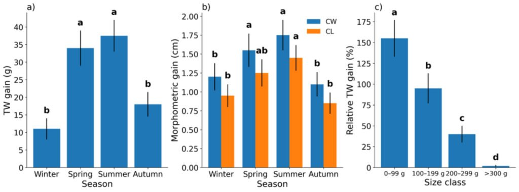
Discussion
The relatively high survival rate can be attributed to the design of the artificial habitat, which included multiple buried shelters, regulated humidity through simulated rainfall, access to both freshwater and saltwater, and low stocking density. These conditions have been recognized as critical factors for terrestrial crab survival under controlled environments (Herreid, 1963; Oliveira et al., 2020), likely contributing to reduced stress, enhanced shelter availability, and overall behavioral stability.
Importantly, no signs of cannibalism or excessive agonistic behavior were observed during the experimental period. This contrasts with other decapods in captivity where confinement and competition for space often lead to significant mortality, as reported by Bauer (1986) and Fox (1975). The lack of mortality peaks during the reproductive season also suggests that the species can tolerate environmental manipulation and semi-controlled conditions without major physiological stress.
To our knowledge, this is one of the first experimental reports documenting long-term survival of C. guanhumi under captive conditions with ecological elements resembling natural mangrove habitats. Previous studies on this species have primarily been limited to short-term reproductive monitoring or natural history observations (Hartnoll, 1982; Smith & Smith, 2001).
Table 1
Summary of survival by sex in Cardisoma guanhumi after 12 months under semi-controlled conditions.
| Sex | Initial number | Final number | Survival (%) |
| Male | 132 | 106 | 80.3 |
| Female | 209 | 154 | 73.7 |
| Combined | 341 | 260 | 76.25 |
No statistical comparisons were performed, as crabs were maintained in a single habitat. However, survival rates by sex are reported for descriptive purposes.
The reproductive performance observed under semi-controlled conditions confirms that C. guanhumi is capable of adapting its reproductive cycle to artificial environments with minimal intervention. The presence of mangrove vegetation, natural soil substrate, and controlled humidity may have played a key role in maintaining environmental cues necessary for ovarian development and spawning behavior, as shown in studies on similar species (Mariappan et al., 2000; Silva & Oshiro, 2002). Unlike studies performed under purely laboratory conditions, where reproductive inhibition is common in terrestrial crabs, this setup offered a more ecologically relevant habitat, favoring reproductive success. The relatively high frequency of ovigerous females obtained without hormonal induction or photoperiod manipulation highlights the potential of C. guanhumi for captive broodstock development. Given the limited number of experimental studies on reproductive ecology in this species, these findings contribute novel evidence for its suitability in aquaculture and conservation-based culture systems.
The observed growth pattern in C. guanhumi under captive conditions may reflect a typical crustacean molting mechanism, in which the inner layer of the old exoskeleton is reabsorbed prior to ecdysis and a new cuticle is secreted and later calcified. This process allows size increase while maintaining structural stability of the carapace in adults. The reabsorption of calcium and other minerals, and their temporary storage in gastroliths or the hepatopancreas, has been well documented in decapods (Chang, 1995; Greenaway, 1985; Skinner, 1985), and is particularly relevant in land crabs due to limited environmental calcium availability.
Although somatic growth in decapod crustaceans is typically associated with molting events, the sustained morphometric increases observed in this study, in the apparent absence of clearly detectable ecdysis, may reflect subtle molting events, mineral recycling dynamics, or cuticular remodeling processes not externally observed. Similar mechanisms have been discussed in other decapods under stable environmental conditions (Chang, 1995; Greenaway, 1985; Skinner, 1985).
This physiological flexibility may represent an adaptive response of semi-terrestrial crabs to fluctuating environmental constraints (Anger, 2013; Zimmer et al., 2019). Further studies incorporating histological and endocrine approaches would help clarify the mechanisms underlying the morphometric patterns recorded here (Hartnoll, 2001). Similar sex-based morphometric assessments have been conducted in other brachyurans such as Menippe mercenaria, where cheliped development is linked to territorial behavior and reproductive strategies (Bauer, 1986; Savage & Sullivan, 1978).
Cardisoma guanhumi can be maintained under semi-controlled conditions with high survival and reproductive performance. The sustained morphometric growth recorded during the study provides a baseline for understanding its physiological responses in captivity and supports its potential for ex situ conservation and aquaculture applications.
Acknowledgments
The authors are grateful to Andrés Cabrera Muñoz from the Aquaculture Genetics and Production Laboratory (ITBOCA) for his technical assistance throughout the study.
References
Alvarez, L. E., & Briquets, L. D. (1983). Growth patterns in the stone crab Menippe mercenaria. Gulf Research Reports, 7, 307–314.
Anger, K. (2013). Adaptations to life in terrestrial and semi-terrestrial environments: a comparative view. Invertebrate Zoology, 10, 305–318.
Bauer, R. T. (1986). Phylogenetic trends in sperm transfer and storage complexity in decapod crustaceans. Journal of Crustacean Biology, 6, 313–325. https://doi.org/10.1163/193724086X00181
Botelho, C. F., Souza, A. T., & Oshiro, L. M. Y. (2001). Growth and survival of Cardisoma guanhumi in controlled environments. Crustacean Research, 30, 15–22.
Chang, E. S. (1995). Physiological and biochemical changes during the molt cycle in decapod crustaceans: an overview. Journal of Experimental Marine Biology and Ecology, 193, 1–14. https://doi.org/10.1016/0022-0981(95)00106-9
Diele, K., Koch, V., & Saint-Paul, U. (2005). Population structure, catch composition and CPUE of the artisanally harvested mangrove crab Ucides cordatus in the Caeté estuary, North Brazil: indications for overfishing. Aquatic Living Resources, 18, 169–178. https://doi.org/10.1051/alr:2005018
Fox, L. R. (1975). Cannibalism in natural populations. Annual Review of Ecology and Systematics, 6, 87–106.
Gifford, C. A. (1963). Some observations on the general biology of the land crab Cardisoma guanhumi. Biological Bulletin, 124, 209–223.
Greenaway, P. (1985). Calcium balance and moulting in the crustacea. Biological Reviews, 60, 425–454. https://doi.org/10.1111/j.1469-185X.1985.tb00424.x
Greenaway, P. (2003). Terrestrial adaptations in crustaceans. In D. R. Lindberg, & R. G. Gillespie (Eds.), Crustaceans and the biodiversity crisis (pp. 823–842). Brill. https://doi.org/10.1163/9789004630543_062
Hartnoll, R. G. (1982). Growth. In D. E. Bliss (Ed.), The Biology of Crustacea, Vol. 2 (pp. 111–196). Nueva York: Academic Press.
Hartnoll, R. G. (2001). Growth in Crustacea —twenty years on. Hydrobiologia, 449, 111–122. https://doi.org/10.1023/A:1017597104367
Herreid, C. F. (1963). Temperature and water relations of the land crab Cardisoma guanhumi. Biological Bulletin, 125, 107–118.
Kristensen, E. (2008). Mangrove crabs as ecosystem engineers; with emphasis on sediment processes. Journal of Sea Research, 59, 30–43. https://doi.org/10.1016/j.seares.2007.05.004
Mariappan, P., Balasundaram, C., & Schmitz, B. (2000). Decapod crustacean chelipeds: an overview. Journal of Biosciences, 25, 301–313. https://doi.org/10.1007/BF02703939
Savage, T., & Sullivan, M. J. (1978). Morphometric analysis of male and female stone crabs (Menippe mercenaria). Florida Scientist, 41, 12–19.
Semarnat (Secretaría de Medio Ambiente y Recursos Naturales). (2020). Norma Oficial Mexicana NOM-059-SEMARNAT-2010. Protección ambiental – Especies nativas de México de flora y fauna silvestres. Diario Oficial de la Federación. Disponible en: https://www.dof.gob.mx/nota_detalle.php?codigo=5173091
Shinozaki-Mendes, R. A., Silva, J. R. F., & Hazin, F. H. V. (2013). Reproductive biology of the land crab Cardisoma guanhumi (Decapoda: Gecarcinidae) in north-eastern Brazil. Journal of the Marine Biological Association of the United Kingdom, 93, 761–768. https://doi.org/10.1017/S0025315412000951
Skinner, D. M. (1985). Molting and regeneration. In D. E. Bliss (Ed.), The Biology of Crustacea, Vol. 9 (pp. 43–146). Nueva York: Academic Press.
Sokal, R. R., & Rohlf, F. J. (2003). Biometry: the principles and practice of statistics in biological research. Nueva York: W. H. Freeman.
Taissoun, R. J. (1974). Mating and sperm storage in female decapods: a strategy for multiple broods. Journal of Crustacean Biology, 1, 325–330.
Watson-Zink, V. M. (2021). Making the grade: physiological adaptations to terrestriality in decapod crabs. Current Opinion in Insect Science, 47, 88–94. https://doi.org/10.1016/j.cois.2021.05.009

Wild chia (Salvia hispanica) populations, endangered under global warming scenarios
Peligro de extinción de poblaciones silvestres de chía (Salvia hispanica) bajo escenarios de calentamiento global
Sabina Lara-Cabrera a, *, Gleisery Rivas-Jaimes a, David A. Prieto-Torres b, c, Cuauhtémoc Sáenz-Romero c, d, Lourdes Núñez-Landa a, Guillermo Orozco-de Rosas e, Juan-Carlos Montero-Castro a
a Universidad Michoacana de San Nicolás de Hidalgo, Facultad de Biología, Laboratorio de Biodiversidad y Biogeografía de Plantas, Gral. Francisco J. Múgica s/n, Ciudad Universitaria, Edificio B2, 3er piso, Felicitas de Río, 58030 Morelia, Michoacán, Mexico
b Universidad Nacional Autónoma de México, Facultad de Estudios Superiores Iztacala, Laboratorio de Biodiversidad y Cambio Climático, Av. de los Barrios 1, Los Reyes Iztacala, 54090 Tlalnepantla, Estado de México, Mexico
c Laboratorio Nacional de Biología del Cambio Climático, SECIHTI, Mexico
d Universidad Michoacana de San Nicolás de Hidalgo, Instituto de Investigaciones sobre los Recursos Naturales, Av. Juanito Itzícuaro s/n, Col. Nueva Esperanza, 58337 Morelia, Michoacán, Mexico
e Chia Blanca, S.C. de R.L., La Paz No. 54, 45470 Acatic, Jalisco, Mexico
*Corresponding author: sabina.lara@umich.mx (S. Lara-Cabrera)
Received: 25 July 2025; accepted: 14 January 2026
Abstract
The conservation of crop wild relatives is particularly worrisome under global warming scenarios given their potential as sources of diversity for cultivars. Here we evaluate the potential effect of climate change through ecological niche modeling for wild chia (Salvia hispanica) populations as the closest crop wild relative. Current and future (2040, 2060, 2080) climatic conditions were modeled using 4 global climate models (ACCESS-CM2, BCC-CSM2-MR, MIROC6, and CanESM5) and 2 shared socioeconomic pathways (SSP2-4.5 and SSP5-8.5), accounting for both limited and long-distance dispersal scenarios. Current potential wild S. hispanica distribution is 192,789 km², 16.72% in climatically stable areas and coinciding with 184 Nature Conservancy Areas in Mexico and Guatemala. Unfortunately, by 2040, 2060, and 2080 wild chia’s potential distribution would reduce by 60.81 to 83.07%, respectively under optimistic scenarios with potential of dispersion as well as pessimistic and nondispersal scenarios. Furthermore, the most sensitive areas are in the Trans-Mexican Volcanic Belt, Pacific Coast, and Guatemala, which also are reportedly the most genetically diverse populations. We urge conservation efforts to increase wild germplasm collections and embark on in situ conservation with local communities to preserve the genetic reservoir of the species for future crop breeding.
Keywords: Climate change; Environmental suitability; Species distribution; Vulnerability risk
Resumen
Una de las mayores preocupaciones ante escenarios de cambio climático es la conservación de parientes silvestres de cultivos, dado su potencial como fuente de diversidad genética. Aquí evaluamos el efecto potencial del cambio climático actual y futuro (2040, 2060, 2080) para poblaciones silvestres de chía (Salvia hispanica), el pariente silvestre más cercano, a través de modelación del nicho ecológico utilizando 4 modelos de cambio climático (ACCESS-CM2, BCC-CSM2-MR, MIROC6 y CanESM5) bajo 2 trayectorias socioeconómicas (SSP2-4.5 y SSP58.5), considerando también dispersión limitada y de larga distancia. La distribución potencial actual de poblaciones silvestres de S. hispanica es de 192,789 km² y 16.72% en áreas climáticamente estables que coinciden con 184 áreas naturales de conservación de México y Guatemala. Desafortunadamente hacia 2040, 2060 y 2080 su distribución se reducirá de -60.81% a -83.70% respectivamente bajo trayectoria socioeconómica optimista con dispersión a larga distancia y pesimista con dispersión limitada. Adicionalmente las regiones más sensibles coinciden con las que se han reportado como genéticamente diversas en el Cinturón Volcánico Trans-Mexicano, Costa del Pacífico y Guatemala. Llamamos a incrementar los esfuerzos de conservación, aumentar las colecciones de germoplasma e iniciar proyectos de conservación in situ comunitarios con miras a conservar el reservorio genético del cultivo.
Palabras clave: Cambio climático; Idoneidad ambiental; Distribución de especies; Riesgo por vulnerabilidad
Introduction
Chia is a native crop of Mesoamerica (Cahill, 2003; Kirchhoff, 2000). Several attributes related to the high omega-3 content of chia (Salvia hispanica L.) have led to its steadily growing global consumption (Ali et al., 2012; Grancieri et al., 2019; Katunzi-Kilewela et al., 2021). While current estimates of global production increased in Paraguay, Bolivia, and Mexico from ca. 13,000,000 in 2019 to 18,000,000 in 2023 (Anuario Estadístico de Producción Agrícola, 2025) and consumption was estimated at 80,000 to 100,000 tons per year (Góral, 2025), little attention has been given to the distribution and conservation of wild chia populations, which are considered a Crop Wild Relative (CWR) and thus an important source of genetic variability for the crop (Maxted et al., 2006). The earliest documentary records, including the “Matrícula de tributos” (2022) and the “Relaciones geográficas de la Nueva España” (Murrieta-Flores et al., 2020), highlight the significance of chia in pre-Hispanic diets, ranking third in importance after maize and beans. However, the timeline of its domestication remains uncertain. The only unequivocal archaeobotanical evidence is nutlets dated to 1,750 years before present. Some studies suggest an earlier domestication event around 4,500 years ago based on pollen records (Sosa et al., 2016), although these may only be assignable to the genus Salvia rather than specifically to S. hispanica (LaraCabrera et al., 2025). Therefore, major questions regarding the identity and timeline of chia’s domestication cannot yet be addressed. Available evidence strongly suggests that domestication occurred in Mexico-Guatemala (i.e., Mesoamerica), a recognized center of origin for many globally important crops (Colunga-García Marín & Zizumbo-Villareal, 2004; Flannery, 1973). Chia has been included in Mexico’s inventory of 310 priority CWR species (Contreras-Toledo et al., 2018) and the global CWR inventory proposed by Harlan and De Wet (Vincent et al., 2013). The closest chia relatives are wild chia populations, making their study and conservation a pressing need. The conservation of CWRs is a global concern, as emphasized by the FAO, which recognizes their critical role in ensuring future food security in the context of global change (Kaeslin et al., 2012). In this context, the first step toward developing effective conservation strategies, as highlighted by Goettsch et al. (2021), is to generate accurate distribution maps, beginning by data curation to remove misidentified records and cultivated specimens. Here we apply ecological niche modeling using Maxent to wild chia populations in order to: 1) approximate the species’ Grinnellian niches (Peterson et al., 2011; Rödder & Engler, 2011); and 2) project future distribution under global warming scenarios (Dormann et al., 2007). Previous work by Durán et al. (2016) modeled environmental suitability for the periods 2041-2060 and 2061-2080, also using herbarium specimens. However, it remains unclear whether they distinguished wild from cultivated specimens, a key factor, as a mixed dataset could affect model accuracy due to differences in abiotic tolerance and dispersal capability. Here we carefully selected only wild chia specimens based on morphological traits, avoiding individuals exhibiting a domestication syndrome. For example, in wild populations, the fruiting calyx remains open, allowing nutlet release whereas in cultivated chia nutlets remain enclosed in the fruiting calyx. Chia nutlets (often misinterpreted as seeds) produce mucilage upon contact with water, and as has been described for thyme, the hydrated mericarp swells and pushes the calyx open to expose the nutlet (Bouman & Meeuse, 1992). Domesticated plants also tend to have larger overall size, inflorescences, and flowers (Cahill, 2003, 2005). Our dataset was subsequently used to model future niche distributions for the years 2040, 2060, and 2080 under optimistic and pessimistic Shared Socioeconomic Pathways (SSPs) following the Intergovernmental Panel on Climate Change (IPCC, 2022), global warming being one of the most severe threats to CWR conservation. We also considered chia’s potential for dispersal and colonization of new areas. Chia likely has limited natural dispersal via water (hydrochory or ombrochory; Zona, 2017), and when calices remain open gravity plays a role as nutlets fall near the parent plant and germinate nearby (phylomatri sensu Cheplick, 2021). Yet long-distance dispersal, potentially through human activity, may become crucial under accelerated climate change. Finally, given the serious conservation threat for many CWRs through land-use change (Goettsch et al., 2021), we evaluated the spatial overlap between the modeled distributions and the Mexican and Guatemalan Natural Conservation Areas. These areas represent an immediate opportunity for passive CWR conservation, especially at biodiversity hotspots where indigenous communities have managed the surrounding species for millennia resulting through domestication in a mosaic of landraces (Vincent et al., 2022). Our results offer valuable guidance for policymakers and plant breeders, enabling the identification of wild chia populations for in situ conservation and seed bank enhancement for ex situ conservation. Early, informed decisions are essential for preserving the genetic diversity of this culturally and nutritionally important crop.
Materials and methods
Biological data acquisition. Occurrence data follow Lara-Cabrera et al. (2025) identifying wild specimens from digitized herbarium collections at the Consortium of California Herbaria ([https://cch2.org/portal/collections/] RSA, UCR) MEXU (https://datosabiertos.unam.mx/ biodiversidad/), Portal Torch Herbaria ([https://portal. torcherbaria.org/portal/index.php] ASU, CIIDIR, COLO, DES, IBUG, IND, MICH, UNM, UTEP, WIS), US (https:// collections.nmnh.si.edu/search/botany/), and herbarium review (IEB). Domestication status was determined based on botanical descriptions (Klitgaard, 2012; Ramamoorthy, 1996; Wood & Harley, 1989) and cross-checked with studies on domestication syndrome traits in the species (Cahill, 2003, 2005; Calderón-Ruíz et al., 2021). Overall, wild specimens are recognized as shorter plants (30-100 cm tall), with short inflorescences (up to 10 cm), bearing 3 to 6 flowers per verticillaster, corolla tube 8-9 mm long that is almost entirely enclosed by the calix, and smaller fruiting calyces remaining open at maturity. Note that the ability to maintain open calyces to release the nutlets is a key trait distinguishing most domesticated varieties, as in the latter the calyx remains closed. All records were carefully reviewed to eliminate ambiguities such as duplicates, points located on roads or residential areas, and records with a spatial separation of less than 2 km to reduce spatial autocorrelation (Boria et al., 2014; Legendre, 1993; Peterson et al., 2011). Following Prieto-Torres et al. (2020, 2021) and PrietoTorres (2024), recent records (2001-2022) were subjected to an environmental outlier exclusion procedure. Records were removed if their values for Worldclim bioclimatic variables Bio 1 (annual mean temperature), Bio 5 (maximum temperature warmest month), Bio 12 (annual precipitation), and Bio 15 (precipitation seasonality) fell outside the upper or lower quartiles of the same variables calculated from herbarium records dated between 19702000. Those variables were used because other studies (e.g., Núñez-Landa et al., 2023; Prieto-Torres et al., 2020, 2021) have found them useful in the data depuration process. The final occurrence dataset included 55 independent localities of species presence, corresponding to the full list published by Lara-Cabrera et al. (2025). Environmental information for current and future scenarios. Available climatic layers were downloaded from Worldclim 2.1 (Fick & Hijmans, 2017; Hijmans et al., 2005) at a spatial resolution of 30 arc-seconds (~ 1 km²). These bioclimatic variables, derived from monthly temperature and precipitation data, reflect longterm climatic trends. Nonetheless, variables Bio 8 (mean temperature wettest quarter), Bio 9 (mean temperature dries quarter), Bio 18 (precipitation of wettest quarter), and Bio 19 (precipitation of coldest quarter) were excluded due to potential spatial artifacts in their interpolated surfaces, which could negatively affect model performance (Booth, 2022; Escobar et al., 2014). Checking for such anomalies is particularly important when modeling across broad regions, as in this study, to prevent localized irregularities which could bias overall results (Booth, 2022). And although soil properties influence species distributions by affecting plant physiology, growth, and survival (Eamus et al., 2013; Velazco et al., 2017), we focused exclusively on climatic variables because no reliable projections of edaphic variables exist for future scenarios (Tomlinson et al., 2020). Moreover, temperature and precipitation strongly influence soil properties, so climatic variables are expected to indirectly capture part of the soil-related variability. This reasoning is consistent with studies highlighting climate as the main driver for long-term distributional shifts (Dantas et al., 2020; Hartmann et al., 2022). To avoid model overfitting due to collinearity among variables (Dormann et al., 2013), we employed a twostep process to select relevant predictors and reduce dimensionality (Cobos et al., 2019). First, Spearman and Pearson correlation coefficients were used to exclude variables with correlations greater than 0.8 and with a variance inflation value greater than 4 (Díaz-Vallejo et al., 2024; Dupin & Smith, 2019). Both coefficients were used because normality tests indicated that each variable could exhibit different spatial patterns, and a single test would not be feasible due to high spatial autocorrelation among variables, thereby justifying the combined use of both correlation measures (Díaz-Vallejo et al., 2024). Second, a principal component analysis (PCA, Janeković & Novak, 2012) was performed on the original 15 climatic variables across the study area to retain those that collectively explained at least 95% of the total variance (Hanspach et al., 2011). These procedures were performed in R using libraries “corplot”; “usdm” (Wei & Simko, 2017), and “ENMGadgets” (Barve & Barve, 2016). The best climatic data approach was selected based on statistical performance evaluated with the “kuenm” R package (Cobos et al., 2019). For future climate projections, we considered 2 Shared Socioeconomic Pathways from the Coupled Model Intercomparison Project (CMIP6): SSP2-4.5, representing a middle-of-the-road scenario with moderate emissions; and SSP5-8.5, a high-emission scenario reflecting continued fossil fuel dependence and rapid economic growth (Riahi et al., 2017). Projections were generated for 3 future timeframes: 2041–2060 (hereafter 2040), 2061– 2080 (hereafter 2060), and 2070-2090 (hereafter 2080), using 4 General Circulation Models: ACCESS-CM2, BCCCSM2-MR, MIROC6, and CanESM5. These models were selected based on their ability to simulate ENSO dynamics and associated interannual variability in precipitation and temperature (Bi et al., 2013; Watanabe et al., 2010; Zelinka et al., 2020), which are key drivers of climate patterns within the range of S. hispanica and and the whole biota of Central American and Mexico. Therefore, this selection ensures that the models capture climate processes directly relevant to the species’ environmental niche and potential distribution (Jin et al., 2025). The environmental variables selected were cropped to a region defined as M used for model calibration processes (Barve et al., 2011; Soberón & Peterson, 2005). The vectorial polygon defining M was constructed by intersecting species occurrence records with maps of terrestrial ecoregions (Dinerstein et al., 2017) and Neotropical Biogeographic provinces (Morrone et al., 2017). Although several valid approaches exist to define the M area in ecological niche modeling, we selected this method because it is not only straightforward but also highly operational (Rojas-Soto et al., 2024). Ecological niche and potential species distribution. Species models were performed with Maxent 3.4.3 (Phillips et al., 2006) and the R package “kuenm” (Cobos et al., 2019). Maxent constructs the most probable species distribution based on presence-only data and environmental variables through machine learning algorithms, as it is recognized as one of the most effective tools in terms of predictive performance (Elith et al., 2006). The “kuenm” R package was used to generate multiple candidate models by combining different sets of environmental variables (non-correlated and PCAreduced) with a range of Maxent calibration parameters (described below) to select the optimal model and subsequently project it to climate scenarios for 2040, 2060, and 2080. Occurrence records were initially split into 2 datasets: 80% were randomly selected for model training, while the remaining 20% were used for internal validation of the final model. During the calibration step, we created spatial folds using 80% of the records for training, and spatial cross-validation was applied. This approach allowed us to test 992 candidate models resulting from all 62 combinations of Maxent feature classes and 8 regularization multipliers (0.2, 0.4, 0.5, 1, 2, 6, 8, 10) and the 2 sets of variables (non-correlated and PCA-derived), in order to select the optimal set for the final modeling (Cobos et al., 2019). Optimal models were selected based on 3 criteria: statistical significance via partial ROC partial test (Peterson et al., 2008), Akaike’s information criterion for small sample sizes (AICc; Akaike, 1974), and an omission rate below 5% (Anderson et al., 2003). Final models were generated using 1,000 iterations and 10 replicates. Next, the models were projected onto future climate scenarios using 3 extrapolation settings: no extrapolation or clamping, extrapolation without clamping, and both extrapolation and clamping. These approaches are essential to identify novel climatic conditions under future scenarios, potentially suitable for the species based on extreme values of ecological variables (Elith et al., 2011; Peterson et al., 2018; Stohlgren et al., 2001). In this context, to detect future regions with non-analogous climatic conditions relative to the present, we implemented the MOP (Mobility-Oriented Parity) test (Owens et al., 2013). This test identifies zones that represent strict extrapolations of the model, which are associated with higher uncertainty and should be interpreted with caution (Alkishe et al., 2017). The Maxent outputs in “cloglog” format were converted to binary presence-absence maps using a threshold equal to the 10th percentile of training presence. This threshold minimizes commission errors by excluding only the lowest 10% of suitability scores, thus retaining predictions considered at least as suitable as the occurrence records (Liu et al., 2013). The binary maps for each Shared Socioeconomic Pathway (SSP2-4.5 and SSP5-8.5) and time period (2040, 2060, and 2080) were generated by overlaying the outputs from 4 selected Atmosphere-Ocean General Circulation Models (ACCES-CM2, BCC-CSM2MR, MIROC6, and CanESM5). Herein, a grid cell was classified as “presence” if at least 3 of the 4 models agreed on the presence prediction for that cell (e.g., Nuñez-Landa et al., 2023; Gama-Rodríguez et al., 2024). Spatial analyses and general metrics. The current binary map was compared with each future projection by overlaying and summing them, to define climatically stable areas, where a cell was considered “climatically stable” if the species’ environmental conditions were predicted therein for all evaluated periods (Collevatti et al., 2013). It is important to note that this does not imply that the local climate remains unchanged, but rather that the cell stays within the species’ tolerable range, allowing potential persistence (Terribile et al., 2012). Identifying such areas is important because they often harbor higher intraspecific genetic diversity (Hewitt, 2004). Besides, a range gain was defined when the number of pixels predicted to be suitable for distribution areas in the future were greater than those estimated in the present, and the opposite case was interpreted as range contraction for the species. Given that a species’ dispersal capacity can influence its ability to colonize new areas (Marco et al., 2011), we conducted this evaluation under 2 contrasting dispersal scenarios: short-distance dispersal (SDD), where suitable future areas were limited to those overlapping with the current distribution, and long-distance dispersal (LDD), where suitable areas projected for the future but not currently occupied were also considered. In both cases, geographic barriers defined by the M area were assumed to limit species dispersal, and ecological interactions between species were omitted (Atauchi et al., 2020; Peterson et al., 2002). For projections predicting a loss of suitable areas, we calculated the differences (current vs. future) in values of the bioclimatic and elevation variables to identify the environmental changes associated with this loss (Cobos & Bosch, 2018; Atauchi et al., 2020). The geographic centroid of the binary maps (for each present and future projections) was computed using the coordinates of all presence-value cells, with the constraint that the centroid must lay within the presence area. To enhance discussion, centroid shift was estimated in all scenarios and temporalities and actual km² and displacement direction estimated in R through the haversine formula proposed by Inman (1835). Additionally, the mean elevation and its range for each temporality were extracted by coupling future climate projection pixels with a digital elevation model. Both analyses were performed with the “terra” R package (Hijmans, 2025) Finally, we assessed the overlap between the current and projected species distribution and Natural Protected Areas (NPAs) in Mexico (https://www.gob. mx/conanp#1692) and Guatemala (https://conap.gob.gt/ listado-de-areas-protegidas/; IUCN & UNEP-WCMC, 2025). This was done by intersecting current and future binary distribution maps with the raster layers of official NPAs to identify key regions where in situ conservation of chia may be crucial in the face of land use change, contributing to risk mitigation through habitat protection.
Results
Current distribution pattern. The potential distribution model for S. hispanica was adequately calibrated, as indicated by the mean AUC ratio (1.85), minimum AIC value (708.46), statistically significant partial ROC test (0.00), and 0 omission error. The default plot produced shows both omission rates and AICc values for all tested models (Supplementary material: Fig. 1). The final model used a regularization multiplier of 2 and included the feature classes quadratic, product, and hinge. The most important variables that define the first principal component (PC1) are Bio1, Bio3, Bio6, Bio11, and Bio12, whereas the second component (PC2) is primarily defined by Bio12, Bio14, Bio15, and Bio17. The estimated current potential distribution area for wild chia is 192,789 km², primarily located across the biogeographic regions of the Sierra Madre Occidental, Trans-Mexican Volcanic Belt, Sierra Madre del Sur, and Sierra Madre de Chiapas, extending into Guatemala (Fig. 1). In Mexico, chia is distributed from the northeastern states (Sonora, Chihuahua, Durango, and Sinaloa), through the western and central regions, and into the southeast (Guerrero, Oaxaca, and Chiapas). To assess average population shift regarding latitude and longitude we estimated the centroid at 21.0367 oN, -102.231 oW (Jalisco Altos Sur, NW Jalisco, Mexico), average elevation 1,971.1 m and elevational range 1708.6 – 2211.3 m (Table 1). A valuable finding is that 11.51% (i.e., 22,206 km²) of the current projected distribution lies within NPAs. In Mexico the current potential distribution overlaps with
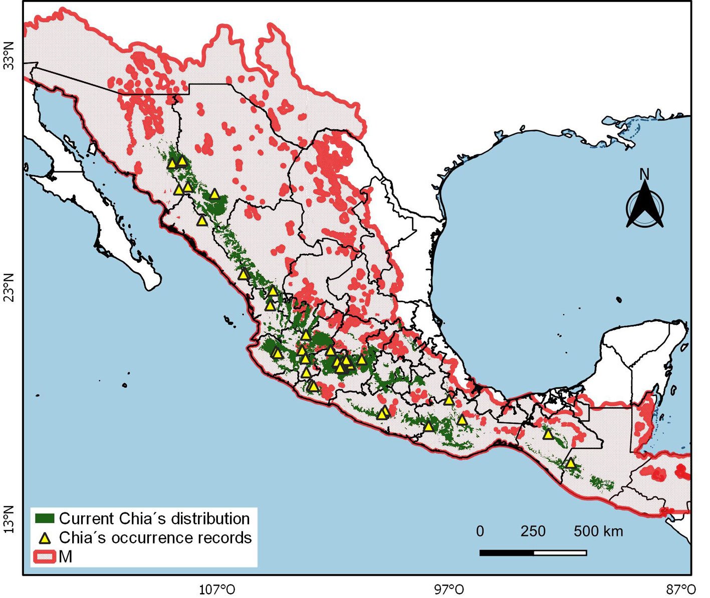
135 NPAs, including 9 Biosphere Reserves (UNESCOMAB), Flora and Fauna Protected Areas, Protected Areas for Natural Resources, National, State, Municipal Parks, and Voluntary Conservation Areas. Whereas in Guatemala the current potential distribution overlaps with 49 areas, including one Biosphere Reserve (UNESCOMAB), Natural Reserves, National and Regional Parks, Definitive Veda Zones, Forest Reserves and Use Reserves (Supplementary material: Table 1). Projected distribution patterns under non-dispersal and dispersal scenarios. The potential distribution of wild S. hispanica populations for 2040, 2060, and 2080, modeled considering non dispersal (i.e., SDD), highlights a concerning and pessimistic trend of habitat loss (Table 1, Fig. 2a). Under the optimistic global warming SSP24.5 scenario, the potential distribution area is projected to lose 38.27% by 2040, 50.07% by 2060 and 60.81% by 2080, leaving only a remaining area of 119,002 km², 96,250 km², and 75,551 km², respectively. In contrast, under the pessimistic warming scenario (SPS5-8.5), the remaining area is expected to be 32,638 km², reflecting a dramatic 83.07% loss of the current distribution. The loss of suitable habitat also extends to populations currently located within NPA: by 2040 only 15,879 km² (i.e., 13.34% of remaining suitability areas) would be within NPA and by 2080 these values are projected to decline further to 11,502 km² (i.e., 15.22%) under the optimistic scenario, and 6,195 km² (18.98%) under the pessimistic one. Furthermore, the geographic centroid of the species’ distribution is expected to shift in both longitude and latitude, accompanied by notable elevational shifts. In the SSP2-4.5 scenario, the mean elevation (currently 1,971.1 m) is projected to increase to 2,246.4 m (range: 2,0572,420.1 m), and to 2,376 m (range: 2,194-2,542.1 m) under SSP5-8.5. This corresponds to an average upward shift in elevation of 275.3 m and 405 m, respectively, along with a contraction of the current elevational range from 503 m to 357 m and 348 m under each scenario. Conversely, under the dispersal scenario (i.e., LDD), the projected future distributions are less alarming, although still indicative of significant habitat changes. These models assume the species eventually could colonize newly suitable areas, although likely requiring human-assisted dispersal. Projected distributions under
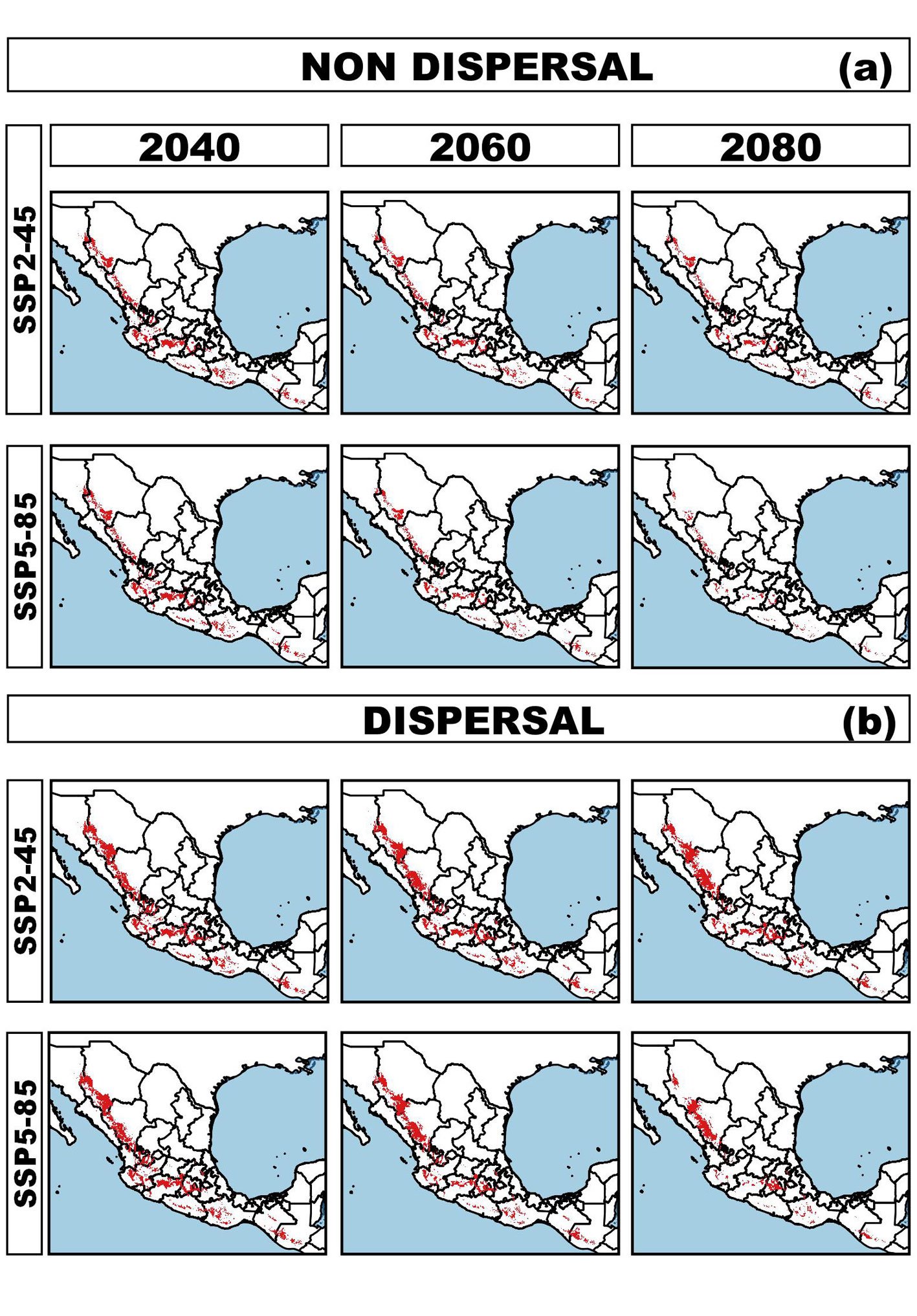
| Models | Potential distribution (pixels / km²) | Within NPA — Pixels (%) | % present vs. future | Change proportion attributable to GCC | Centroid displacement (km) and direction | Average elevation (m) | Min. elevation (m) | Max. elevation (m) |
|---|---|---|---|---|---|---|---|---|
| Current | 192,789 | 22,206 (11.51) | – | – | 21.0367, -102.231 | 1,971.1 | 1,708.6 | 2,211.3 |
| 2040 SSP2-4.5 | 119,002 | 15,879 (13.34) | 8.24 | -38.27 | 76.51 towards NW | 2,126.7 | 1,912.6 | 2,324.5 |
| 2060 SSP2-4.5 | 96,250 | 13,701 (14.23) | 7.1 | -50.07 | 81.13 towards NW | 2,184.9 | 1,984.1 | 2,372.2 |
| 2080 SSP2-4.5 | 75,551 | 11,502 (15.22) | 5.9 | -60.81 | 89.8 towards N-NW | 2,246.4 | 2,057 | 2,420.1 |
| 2040 SSP5-8.5 | 117,304 | 15,622 (13.32) | 8.1 | -39.15 | 14.71 towards SW | 2,130.4 | 1,915.5 | 2,329.6 |
| 2060 SSP5-8.5 | 77,794 | 12,060 (15.50) | 6.3 | -59.65 | 90.63 towards N-NW | 2,233 | 2,035.2 | 2,413.6 |
| 2080 SSP5-8.5 | 32,638 | 6,195 (18.98) | 3.2 | -83.07 | 84.18 towards N-NW | 2,376 | 2,194 | 2,542.1 |
| Models | Potential distribution (pixels / km²) | Within NPA — pixels (%) | % present vs. future | Change proportion attributable to GCC | New area — pixels / km² | New area — % | Centroid displacement (km) and direction | Average elevation (m) | Min. elevation (m) | Max. elevation (m) |
|---|---|---|---|---|---|---|---|---|---|---|
| Current | 192,789 | 22,206 (11.51) | – | – | – | – | 21.0367, -102.231 | 1,971.1 | 1,708.6 | 2,211.3 |
| 2040 SSP2-4.5 | 145,180 | 19,217 (13.24) | 9.96 | -24.69 | 26,178 | 18.03 | 114.4 towards NNW | 2,182.8 | 1,960.6 | 2,390.6 |
| 2060 SSP2-4.5 | 137,076 | 19,513 (14.24) | 10.12 | -28.90 | 40,826 | 29.78 | 140.85 towards NW | 2,277.5 | 2,065 | 2,475.4 |
| 2080 SSP2-4.5 | 125,364 | 18,474 (14.74) | 9.58 | -34.97 | 49,813 | 39.73 | 151.64 towards NW | 2,365.1 | 2,173.8 | 2,542.3 |
| 2040 SSP5-8.5 | 149,217 | 19,778 (13.25) | 10.25 | -22.60 | 31,913 | 21.39 | 117.54 towards NNW | 2,197.8 | 1,972.1 | 2,409.6 |
| 2060 SSP5-8.5 | 123,825 | 18,499 (14.94) | 9.59 | -35.77 | 46,031 | 37.17 | 127.45 towards NNW | 2,341.8 | 2,141 | 2,527.1 |
| 2080 SSP5-8.5 | 78,662 | 14,117 (17.95) | 7.3 | -59.20 | 46,024 | 37.17 | 202.01 towards NW | 2,508.4 | 2,346.2 | 2,655.3 |
Projected distributions under both SSP2-4.5 and SSP5-8.5 scenarios are relatively similar (Table 2, Fig. 2b). Under SSP2-4.5, the species is projected to lose 24.69% of its current range (remaining area: 145,180 km²), while gaining approximately 26,178 km² (18.03%) of new areas by 2040. However, by 2080, only 65% of suitable habitat will persist, with a loss of 35% of the area. Moreover, the proportion of the species’ range within NPAs is also projected to decline under dispersal scenarios, from current potential distribution to future: 18,474 km² (i.e., 9.58% of remaining areas) under SSP2-4.5 and 14,117 km² (i.e., 7.3%) under SSP5-8.5 by 2080. Projected centroid shifts (Table 2) are expected to be up to 114.4 km towards the N-NW and 151.64 km NW by 2080 (S-SW state of Zacatecas), with an optimal elevation rising to 2,365.1 m on average (range: 2,173.8–2,542.3 m) under the optimistic scenario. Under a pessimistic scenario the projected centroid would shift 117.54 km towards N-NW and by 2080 up to 202.01 km towards the NW. We estimated a shift of 2,508.4 m (range: 2,346.2–2,655.3 m), reflecting an upward elevational gain of 394 m to 537.3 m, and a narrowing range of the elevation from 503 m to 364 m and 309 m, respectively.
Long-term climatically stable areas and environmentally driven area loss. Modeled area loss by 2040 and 2080 under a pessimistic scenario was primarily driven by increases in temperature and changes in precipitation regimes (Table 3). Average annual temperature is projected to increase in 1.61 to 4.15 °C, with similar increases for the warmest month (+1.84 to +4.77 °C) and the coolest month (+1.49 to +3.78 °C). Annual and seasonal precipitation are expected to increase slightly (+33.97 to +9.77 mm; +2.10 to +2.64%) from current levels, while precipitation is projected to decrease in the driest quarter (0.92 to 3.18 mm). Under pessimistic scenarios, environmentally suitable areas for species are associated with elevated temperature values across multiple climatic variables, including average annual temperature (+1.83 to +4.17 °C), maximum temperature of the warmest month (+1.83 to +4.78 °C), and minimum temperature of the coldest month (+1.49 to +3.78 °C). The coefficient of variation for seasonal precipitation also increases moderately (+2.14 to +2.91%), while specific reductions are projected for the driest quarter (0.93 to 3.31 mm) compared to current conditions. This seasonal imbalance suggests harsher conditions during warm and dry periods, despite total precipitation increases.
Finally, the climatically stable area suitable for S. hispanica was estimated to be 32,245 km², representing only 16.72% of its total current distribution area (Fig. 3). In Mexico, these stable areas (representing 15.5% of total estimated sites) are located primarily in the northwest (states of Chihuahua and Durango), west (Jalisco and Michoacán), central south (Estado de México, Mexico City, and Guerrero), and southern regions (Oaxaca and Chiapas).
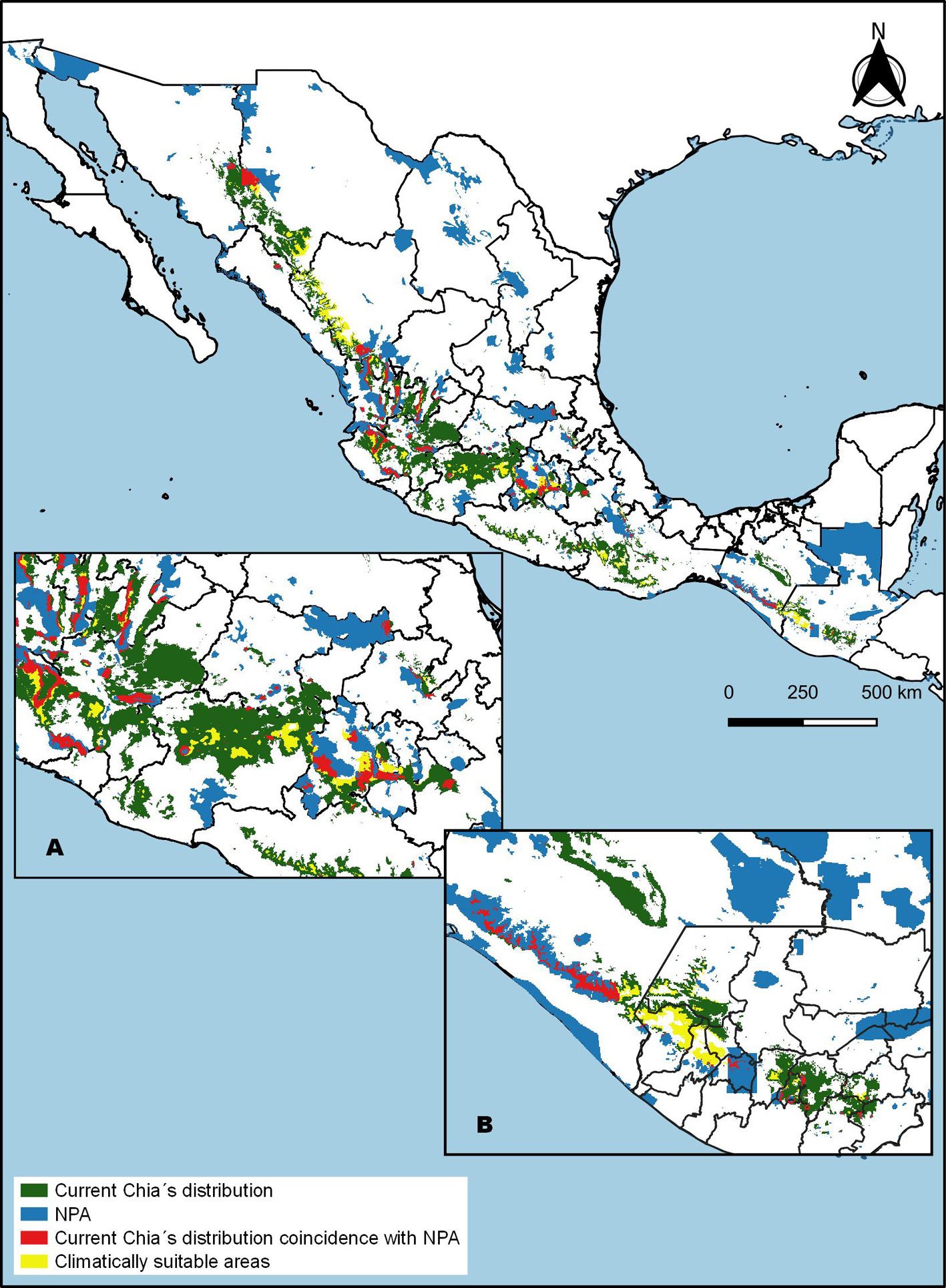
| Variable | SSP2-4.5 (Optimistic scenario) | SSP5-8.5 (Pessimistic scenario) | ||||
|---|---|---|---|---|---|---|
| 2040 | 2060 | 2080 | 2040 | 2060 | 2080 | |
| bio 1 Annual mean temperature (°C) | +1.61 | +2.71 | +4.15 | +1.61 | +2.71 | +4.17 |
| bio 2 Mean diurnal range (mean of monthly (max temp − min temp)) (°C) | +0.07 | +0.21 | +0.41 | +0.07 | +0.20 | +0.41 |
| bio 3 Isothermality (BIO2 / BIO7) (× 100) | -0.55 | -0.76 | -0.89 | -0.55 | -0.78 | -0.91 |
| bio 4 Temperature seasonality (standard deviation × 100) | -1.65 | +0.59 | +4.50 | -1.71 | +0.45 | +4.20 |
| bio 5 Max temperature of warmest month (°C) | +1.84 | +3.13 | +4.77 | +1.83 | +3.14 | +4.78 |
| bio 6 Min temperature of coldest month (°C) | +1.49 | +2.49 | +3.78 | +1.49 | +2.49 | +3.78 |
| bio 7 Temperature annual range (BIO5−BIO6) (°C) | +0.34 | +0.64 | +0.99 | +0.34 | +0.64 | +1.00 |
| bio 10 Mean temperature of warmest quarter (°C) | +1.58 | +2.73 | +4.20 | +1.58 | +2.72 | +4.20 |
| bio 11 Mean temperature of coldest quarter (°C) | +1.62 | +2.70 | +4.09 | +1.62 | +2.71 | +4.11 |
| bio 12 Annual precipitation (mm) | +33.97 | +27.62 | +9.77 | +34.76 | +29.44 | +11.39 |
| bio 13 Precipitation of wettest month (mm) | +16.74 | +16.39 | +12.97 | +16.93 | +16.88 | +14.36 |
| bio 14 Precipitation of driest month (mm) | -0.10 | -0.38 | -0.66 | -0.10 | -0.40 | -0.72 |
| bio 15 Precipitation seasonality (coefficient of variation) (%) | +2.10 | +2.41 | +2.64 | +2.14 | +2.53 | +2.91 |
| bio 16 Precipitation of wettest quarter (mm) | +22.52 | +18.74 | +2.34 | +23.28 | +20.44 | +4.86 |
| bio 17 Precipitation of driest quarter (mm) | -0.92 | -1.95 | -3.18 | -0.93 | -2.00 | -3.31 |
| Climatically stable areas in km² | 32,245 | |||||
| % | 16.72 | |||||
Discussion
Here we report a concerning scenario for the persistence of wild chia populations in the face of global warming through a Species Distribution pipeline employed in Maxtent. Although other pipelines are available such as the use of Random Forests (Breiman, 2001), we were unable to employ it because it requires an even number both of species presences and species absences, which is difficult since usually the latter is many folds larger than the number of presences (Gómez-Pineda et al., 2020). Nevertheless, our resulting hypotheses are robust following current scientific criteria and could serve as a starting point to guide conservation of this CWR for in field follow up to monitor wild chia populations, to reassess proposed abiotic variables and soil interacting agents to fine tune critical variables, and to enhance hypotheses and assure assisted migration success if implemented. Climate change poses imminent threats to individuals, species, and ecosystems (Kaeslin et al., 2012), and the conservation of CWRs is directly linked to future food security. The projected future distribution scenarios for 2040, 2060, and 2080 indicate a dramatic decline in the extent of suitable habitats for wild chia populations; even under the most optimistic scenario area loss is projected. We also foresee a geographic shift in the species’ average longitude and latitude climatic niche, along with a sharp net contraction in elevational range, where the lower elevation limit of the current natural range is expected to suffer larger losses; this finding agrees with projections for many other wild plant species through Mexican mountain gradients (Ramírez-Barahona et al., 2025). The speed of climatic change, exacerbated by the current acceleration of this process (Hansen et al., 2025), makes it highly unlikely that natural populations could disperse their seeds and establish new populations at the locations where suitable climatic conditions will emerge at the required pace. In other words, the mismatch between the areas currently occupied by wild populations and the shifting climate suitable for them will increase over time. Human-assisted translocation of seeds would likely be necessary to ensure species persistence. On the other hand, so-called “climatically stable” areas should not be interpreted with undue optimism. The persistence of an area within the species’ overall climatic niche does not imply that local conditions remain unchanged. This distinction is important when considering populations with significant genetic differentiation in traits such as frost resistance or drought tolerance. Specific populations may remain within the species’ broad climatic niche but become uncoupled from the narrow climate interval to which they have evolved and specialized, as demonstrated for wild forest tree populations along environmental gradients (Ortiz-Bibian et al., 2017; Rehfeldt et al., 2018). All these results add S. hispanica to the growing list of CWRs at risk. For instance, Jarvis et al. (2008) projected climate change effects on the conservation of wild relatives of peanuts (Arachis), potato (Solanum), and cowpea (Vigna), emphasizing the urgency of preserving their natural habitats and, in extreme cases, collecting and storing their genetic material in germplasm banks. Alarmingly, wild populations in the Trans-Mexican Volcanic Belt, a region of highest reported genetic diversity for chia (Cahill, 2004), are expected to be completely lost. Our global climate change scenarios differ markedly from those reported by Durán et al. (2016), who projected an increase in the potential distribution of S. hispanica (chia) under future climate conditions. Overall, they interpreted global climate change as potentially beneficial for the species, predicting moderate to high environmental suitability for 2060 and 2080, and an expansion of suitable areas across central and southern Mexico (Durán et al., 2016). Direct comparison between both studies is difficult due to several methodological differences, including the source of occurrence records (wild-only vs. potentially mixed wild and cultivated), variation in raster resolution (2.5 arc-minutes vs. our 30 arc-seconds), and differences in environmental variables. While we relied solely on bioclimatic variables from WorldClim, Durán et al. (2016) supplemented these data with elevational information from SIAN (translated as Environmental Information System) at INIFAP (National Institute of Forestry, Agriculture and Livestock Research) and photoperiod. Unlike Durán et al. (2016), we did not include elevation. Elevation could be considered a surrogated variable of Mean Annual Temperatures and related temperature variables. There is a strong correlation between temperature and elevation along elevational gradients, at a lapse rate of approximately 0.5 oC for each 100 m of elevational difference (Sáenz-Romero et al., 2010). However, when the species has extensive latitudinal distribution (as in this case) the correlation temperature-elevation will vary and thus, adding elevation as an environmental variable could have confounded effects. Nonetheless, both studies converge in predicting habitat loss in northeastern Mexico, and project similar temperature increases: Durán et al. (2016) estimated an average temperature rise of 1 to 3 oC, while our models predict an average temperature increase of 2.28 oC, ranging from 1.61 to 4.16 oC over the average. Additionally, our projections indicate a mean annual precipitation increase, although it is extremely important to realize that such change has a strong seasonal component. Actual precipitation increase is projected only for the wettest quarter; meanwhile, there is a net decrease of precipitation in all the other quarters. Thus, the total annual precipitation increase is not necessarily beneficial for the biology of the species, since the dry season becomes both drier and warmer. The balance between temperature and rainfall variables are critical for the species’ survival and ecological performance (Böhning-Gaese et al., 2008; Uribe, 2015). Although our study focused exclusively on wild populations of chia as a CWR, it is relevant to note that projections for chia cultivation in Mexico by 2040-2069 (Orozco de Rosas et al., 2014) predict an expansion of suitable areas, particularly in the highlands of Sinaloa, Nuevo León, Tamaulipas, Veracruz, Nayarit, Jalisco, Michoacán, Guerrero, Oaxaca, Morelos, Puebla, and Chiapas. These findings do not contradict our results, as they reflect different environmental requirements between wild and cultivated chia (Chen et al., 2017). Unfortunately, if the CWRs are lost, new characters would not be available to transfer into the cultivars, as has been the case in other crops, such as resistance to pests [from Solanum demissum Lindl. (Díaz-García et al., 2023) to potatoes; from Solanum peruvianum L., Solanum cheesmanii (L.Riley) Fosberg, and Solanum pennellii Correll to tomatoes (Rick & Chetelat, 1995)]; cytoplasmic male sterility in sunflowers (Hajjar & Hodgkin, 2007); and tolerance to drought and salinity in tomatoes (Solanum chilense (Dunal) Reiche and S. pennellii (Rick & Chetelat, 1995) among other traits (see Hajjar & Hodgkin, 2007 for further information). To date, most breeding efforts in chia have focused on mutation induction via radiation (Jamboonsri et al., 2012; Sorondo, 2017), and the full potential of wild relatives remains largely unexplored. Although no severe pestrelated threats have yet been reported for chia cultivars, global warming is enabling the emergence of new pests in many crops (Srinivasa et al., 2022), and chia may face similar risks in the near future. Therefore, we need to be prepared. For example, in Ghana, where chia is cultivated to alleviate hunger in low-income communities due to its low production costs and high nutritional value, several pest infections have already been reported, including coreid bugs (Lagria sp.), Zonocerus variegatus L., Diopsis macrophthalma Dalman (reported as the synonym Diopsis thoracica Westwood) and Fusarium wilt (Yeboah et al., 2014). In Mexico, chia’s center of origin, stem damage by Diabrotica speciosa (Germar), 1824 (Coleoptera) has been shown to reduce seed yield by up to 43% (Sosa-Baldivia & Ruiz-Ibarra, 2016). Interestingly, Salvia karwinskii Benth., a taxonomically close wild relative of chia, was reported to exhibit strong antifeedant activity against Spodoptera littoralis (Boisduval) and Diabrotica virgifera virgifera Leconti (Esquivel et al., 1996), highlighting the value of conserving wild taxa. Beyond climate change, other threats must be addressed to ensure effective in situ conservation of wild chia populations. Among these, land-use change related to anthropogenic activities is particularly severe and rapidly accelerating (Davison et al., 2021; Goettsch et al., 2021; Villaseñor et al., 2024). Although we were unable to model this factor directly, chia’s habitat loss has been documented since 2003 in regions such as Huehuetenango (Guatemala) and in the Mexican states of Jalisco, Colima, and Michoacán (Cahill, 2003) mainly due to overgrazing, land-use transformation to agricultural or residential, herbicide application in nearby monocultures, and induced or accidental burning (personal observations GOR). The current rates of habitat loss and degradation are even more dramatic, particularly due to transformation of pineoak woodlands, which are rich in Salvia species -other CWRs- (Cornejo-Tenorio & Ibarra-Manríquez, 2011; Lara-Cabrera et al., 2016). A hopeful sign is the overlap between the projected distribution of wild chia and existing conservation areas in Mesoamerica. As with other CWRs, these protected areas could serve as strongholds for in situ conservation (Tobón-Niedfeld et al., 2022). And although CWRs are not commonly used to define protected areas, they have been employed in specific cases, as in the establishment of the Sierra de Manantlán Biosphere Preserve to protect the corn wild relative Zea diploperennis (Guzmán & Iltis, 1991). New protected areas could be established to preserve the ca. 100 Mesoamerican CWRs threathened with extinction (Goettsch et al., 2021). Therefore, integrating CWR monitoring into conservation area management is a valuable recommendation (Vincent et al., 2022). Fortunately, wild chia currently occurs, and is expected to persist, within some of the most emblematic Biosphere Reserves in Mexico and Guatemala. We recommend in situ conservation managed by local communities, who have cultivated and utilized chia for over 3,000 years; this should be complemented by ex situ strategies, such as establishing germplasm banks that ensure adequate sampling of wild populations. However, access to this material must be regulated to protect local interests assuming The International Treaty on Plant Genetic Resources for Food and Agriculture (https://www. fao.org/plant-treaty/overview/text-treaty/en). Also, ex situ conservation could involve cultivating wild populations in areas projected to remain suitable or those that would emerge as new suitable areas (in general at higher elevations than today) under future climate scenarios, as proposed for other rare and endangered Mexican plant species (Mendoza-Maya et al., 2022).
Acknowledgements
The first author acknowledges financing through the Secretaría de Ciencias, Humanidades, Tecnología e Innovación: Project 319466; Coordinación de la Investigación Científica, Universidad Michoacana de San Nicolás de Hidalgo. We also thank Joseph Cahill for access to his data set, Yocupitzia Ramírez Amezcua for fruitful discussions, Pedro Chamu for plant collections, and Geraldine Murillo and David Lomeli who participated in data set depuration.
References
Akaike, H. (1974). A new look at the statistical model identification. In IEEE Transactions on Automatic Control, 19, 716–723. https://doi.org/10.1109/TAC.1974.1100705
Ali, N. M., Yeap, S. K., Ho, W. Y., Beh, B. K., Tan, S. W., & Tan, S. G. (2012). The promising future of chia, Salvia hispanica L. Journal of Biomedicine and Biotechnology, 2012, 171956. https://doi.org/10.1155/2012/171956
Alkishe, A. A., Peterson, A. T., & Samy, A. M. (2017). Climate change influences on the potential geographic distribution of the disease vector tick Ixodes ricinus. Plos One, 12, e0189092. https://doi.org/10.1371/journal.pone.0189092
Anderson, R., Lew, D., & Peterson, A. T. (2003). Evaluating predictive models of species distributions: criteria for selecting optimal models. Ecological Modelling, 162, 211–232. https://doi.org/10.1016/S0304-3800(02)00349-6
Anuario Estadístico de Producción Agrícola. (2025). Servicio de información Agroalimentaria y Pesquera. Gobierno de México. Retrieved June 12, 2025 from: https://nube.agricultura.gob.mx/cierre_agricola/
Atauchi, P. J., Aucca-Chutas, C., Ferro, G., & Prieto-Torres, D. A. (2020). Present and future potential distribution of the endangered Anairetes alpinus (Passeriformes: Tyrannidae) under global climate change scenarios. Journal of Ornithology, 161, 723–738. https://doi.org/10.1007/s10336-020-01762-z
Barve, N., & Barve, V. (2016). ENMGadgets: tools for pre and post processing in ENM workflow. R package version 0.0.14. Available from: https://github.com/narayanibarve/ENMGadgets
Barve, N., Barve, V., Jiménez-Valverde, A., Lira-Noriega, A., Maher, S. P., Peterson, A. T. et al. (2011). The crucial role of the accessible area in ecological niche modeling and species distribution modeling. Ecological Modelling, 222, 1810–1819. https://doi.org/10.1016/j.ecolmodel.2011.02.011
Bi, D., Dix, M., Marsland, S., O’Farrell, S., Rashid, H., Uotila, P. et al. (2013). The ACCESS coupled model: description, control climate and evaluation. Australian Meteorological and Oceanographic Journal, 63, 41–64. https://doi.org/10.1071/ES13004
Böhning-Gaese, K., Jetz, W., & Schaefer, H. C. (2008). Impact of climate change on migratory birds: community reassembly versus. Global Ecology and Biogeography, 17, 38–49. https://doi.org/10.1111/j.1466-8238.2007.00341.x
Booth, T. H. (2022). Checking bioclimatic variables that combine temperature and precipitation data before their use in species distribution models. Austral Ecology, 47, 1506–1514. https://doi.org/10.1111/aec.13234
Boria, R. A., Olson, L. E., Goodman, S. M., & Anderson, R. P. (2014). Spatial filtering to reduce sampling bias can improve the performance of ecological niche models. Ecological Modelling, 275, 73–77. https://doi.org/10.1016/j.ecolmodel.2013.12.012
Bouman, F., & Meeuse, A. D. J. (2012). Dispersal in Labiatae. In R. M. Harley, & T. Reynolds (Eds.), Advances in Labiatae Science. Royal Botanic Gardens (pp. 193–202). Kew, UK.
Breiman, L. (2001). Random forests. Machine Learning, 45, 5–32. https://doi.org/10.1023/A:1010933404324
Cahill, J. P. (2003). Ethnobotany of chia, Salvia hispanica L. (Lamiaceae). Economic Botany, 57, 604–618. https://doi.org/10.1663/0013-0001(2003)057[0604:EOCSHL]2.0.CO;2
Cahill, J. P. (2004). Genetic diversity among varieties of Chia (Salvia hispanica L.). Genetic Resources and Crop Evolution, 51, 773–781. https://doi.org/10.1023/B:GRES.0000034583.20407.80
Cahill, J. P. (2005). Human selection and domestication of chia (Salvia hispanica L.) Journal of Ethnobiology, 25, 155–174. https://doi.org/10.2993/0278-0771_2005_25_155_hsadoc_2.0.co_2
Calderón-Ruíz, A., Montes-Hernández, S., García-Perea, M. A., Covarrubias-Prieto, J., Aguirre-Mancilla, C. L., & Raya-Pérez, J. C. (2021). Caracterización de poblaciones de Chía silvestre y cultivada. Revista Mexicana de Ciencias Agrícolas, 12, 1161–1170. https://doi.org/10.29312/remexca.v12i7.2243
Chen, Y. H., Shapiro, L. R., Benrey, B., & Cibrián-Jaramillo, A. (2017). Back to the origin: in situ studies are needed to understand selection during crop diversification. Frontiers in Ecology and Evolution, 5, 125. https://doi.org/10.3389/fevo.2017.00125
Cheplick, G. P. (2022). Philomatry in plants: Why do so many species have limited seed dispersal? American Journal of Botany, 109, 29–45. https://doi.org/10.1002/ajb2.1791
Cobos, M. E., Peterson, A. T., Barve, N., & Osorio-Olvera, L. (2019). kuenm: an R package for detailed development of ecological niche models using Maxent. PeerJ, 7, e6281. https://doi.org/10.7717/peerj.6281
Cobos, M. E., & Bosch, R. A. (2018) Recent and future threats to the Endangered Cuban toad Peltophryne longinasus: potential additive impacts of climate change and habitat loss. Oryx, 52, 116–125. https://doi.org/10.1017/S0030605316000612
Collevatti, R. G., Terribile, L. C., de Oliveira, G., Lima-Ribeiro, M. S., Nabout, J. C., Rangel, T. F. et al. (2013). Drawbacks to palaeodistribution modeling: The case of South American seasonally dry forests. Journal of Biogeography, 40, 345–358. https://doi.org/10.1111/jbi.12005
Colunga-García Marín, P., & Zizumbo-Villarreal, D. (2004). Domestication of plants in Maya lowlands. Economic Botany, 58, S101-S110.
Contreras-Toledo, A. R., Cortés-Cruz, M. A., Costich, D., Rico-Arce, M De L., Brehm, J. M., & Maxted, N. (2018). A crop wild relative inventory for Mexico. Crop Science, 58, 1292–1305. https://doi.org/10.2135/cropsci2017.07.0452
Cornejo-Tenorio, G., & Ibarra-Manríquez, G. (2011). Diversidad y distribución del género Salvia (Lamiaceae) en Michoacán, México. Revista Mexicana de Biodiversidad, 82, 1279–1296.
Dantas, B. F., Moura, M. S. B., Pelacani, C. R., Angelotti, F., Taura, T. A., Oliveira, G. M. et al. (2020). Rainfall, not soil temperature, will limit the seed germination of dry forest species with climate change. Oecologia, 192, 529–541. https://doi.org/10.1007/s00442-019-04575-x
Davison, C. W., Rahbek, C., & Morueta-Holme, N. (2021). Land-use change and biodiversity: Challenges for assembling evidence on the greatest threat to nature. Global Change Biology, 27, 5414–5429. https://doi.org/10.1111/gcb.15846
Díaz-García, G., Enciso-Maldonado, G. A., & Lozoya-Saldaña, H. (2023). Solanum demissum Lindl. in potato breeding. Revista Chapingo. Serie Horticultura, 29, 131–148. https://doi.org/10.5154/r.rchsh.2023.01.001
Díaz-Vallejo, M., Peña-Peniche, A., Mota-Vargas, C., Piña-Torres, J., Valencia-Rodríguez, D., Rangel-Rivera, C. E. et al. (2024). Analyses of the variable selection using correlation methods: an approach to the importance of statistical inferences in the modeling process. Ecological Modelling, 498, 110893. https://doi.org/10.1016/j.ecolmodel.2024.110893
Dinerstein, E., Olson, D., Joshi, A., Vynne, C., Burgess, N. D., Wikramanayake, E. P. et al. (2017). An ecoregion-based approach to protecting half the terrestrial realm. Bioscience, 67, 534–545. https://doi.org/10.1093/biosci/bix014
Dormann, C. F., Elith, J., Bacher, S., Buchmann, C., Carl, G., Carré, G. et al. (2013). Collinearity: A review of methods to deal with it and a simulation study evaluating their performance. Ecography, 36, 027–046. https://doi.org/10.1111/j.1600-0587.2012.07348.x
Dupin, J., & Smith, S. D. (2019). Integrating historical biogeography and environmental niche evolution to understand the geographic distribution of Datureae. American Journal of Botany, 106, 667–678. https://doi.org/10.1002/ajb2.1281
Durán, N., Ruiz, J. A., González, D. R., Mena, S., & Orozco-de Rosas, G. (2016). Cambio climático y su impacto sobre la aptitud ambiental y distribución geográfica de Salvia hispanica L. en México. Interciencia, 41, 407–413.
Eamus, D., Boulain, N., Cleverly, J., & Breshears, D. D. (2013). Global change-type drought-induced tree mortality: Vapor pressure deficit is more important than temperature per se in causing decline in tree health. Ecology and Evolution, 3, 2711–2729.
Elith, J., Graham, C. H., Anderson, R. P., Dudík, M., Ferrier, S., Guisan, A. et al. (2006). Novel methods improve prediction of species’ distributions from occurrence data. Ecography, 29, 129–151. https://doi.org/10.1111/j.2006.0906-7590.04596.x
Elith, J. E., Phillips, S. J., Hastie, T., Dudík, M., Chee, Y. E., & Yates, C. J. (2011). A statistical explanation of Maxent for ecologists. Diversity and Distributions, 17, 43–57. https://doi.org/10.1111/j.1472-4642.2010.00725.x
Escobar, L. E., Lira-Noriega, A., Medina-Vogel, G., & Peterson, A. T. (2014). Potential for spread of the white-nose fungus (Pseudogymnoascus destructans) in the Americas: Use of Maxent and NicheA to assure strict model transference. Geospatial Health, 9, 221–229. https://doi.org/10.4081/gh.2014.19
Esquivel, B., Calderón, J. S., Sánchez, A. A., Ramamoorthy, T. P., Flores, E. A., & Domínguez, R. M. (1996). Recent advances in phytochemistry and biological activity of Mexican Labiatae. Revista Latinoamericana de Química, 24, 44–64.
Fick, S. E., & Hijmans, R. J. (2017). WorldClim 2: new 1 km spatial resolution climate surfaces for global land areas. International Journal of Climatology, 37, 4302–4315. https://doi.org/10.1002/joc.5086
Gama-Rodríguez, A. M., García, J. A., Lozano, L. F., & Prieto-Torres, D. A. (2024). Protecting breeding sites: a critical goal for the conservation of the golden eagle in Mexico under global change scenarios. Journal of Ornithology, 165, 1–17. https://doi.org/10.1007/s10336-024-02168-x
Goettsch, B., Urquiza-Haas, T., Koleff, P., Acevedo-Gasman, F., Aguilar-Meléndez, A., Alavez, V. et al. (2021). Extinction risk of Mesoamerican crop wild relatives. Plants, People, Planet, 3, 775–795. https://doi.org/10.1002/ppp3.10225
Gómez-Pineda, E., Sáenz-Romero, C., Ortega-Rodríguez, J. M., Blanco-García, A., Madrigal-Sánchez, X., Lindig-Cisneros, R. et al. (2020). Suitable climatic habitat changes for Mexican conifers along altitudinal gradients under climatic change scenarios. Ecological Applications, 30, e02041. https://doi.org/10.1002/eap.2041
Góral, P. (2025). Chia seeds market update – January 2025. Retrieved June 12, 2025.
Grancieri, M., Martino, H. S. D., & González-de Mejía, E. (2019). Chia seed (Salvia hispanica L.) as a source of proteins and bioactive peptides with health benefits: a review. Comprehensive Reviews in Food Science and Food Safety, 18, 480–499. https://doi.org/10.1111/1541-4337.12423
Guzmán, R., & Iltis, H. H. (1991) Biosphere reserve established in Mexico to protect rare maize relative. Diversity, 7, 82–84.
Hajjar, R., & Hodgkin, T. (2007). The use of wild relatives in crop improvement: a survey of developments over the last 20 years. Euphytica, 156, 1–13. https://doi.org/10.1007/s10681-007-9363-0
Hansen, J. E., Kharecha, P., Sato, M., Tselioudis, G., Kelly, J., Bauer, S. E. et al. (2025) Global warming has accelerated: Are the United Nations and the public well-informed? Environment: Science and Policy for Sustainable Development, 67, 6–44. https://doi.org/10.1080/00139157.2025.2434494
Hartmann, H., Bastos, A., Das, A. J., Esquivel-Muelbert, A., Hammond, W. M., Martínez-Vilalta, J. et al. (2022). Climate change risks to global forest health: emergence of unexpected events of elevated tree mortality worldwide. Annual Review of Plant Biology, 73, 673–702. https://doi.org/10.1146/annurev-arplant-102820-012804
Hanspach, J., Kühn, I., Schweiger, O., & Pompe, S. (2011). Geographical patterns in prediction errors of species distribution models. Global Ecology and Biogeography, 20, 779–788. https://doi.org/10.1111/j.1466-8238.2011.00649.x
Hewitt, G. M. (2004). Genetic consequences of climatic oscillations in the Quaternary. Philosophical Transactions of the Royal Society of London. Series B: Biological Sciences, 359, 183–195. https://doi.org/10.1098/rstb.2003.1388
Hijmans, R. J., Cameron, S. E., Parra, J. L., Jones, P. G., & Jarvis, A. (2005). Very high resolution interpolated climate surfaces for global land areas. International Journal of Climatology: A Journal of the Royal Meteorological Society, 25, 1965–1978. https://doi.org/10.1002/joc.1276
Hijmans, R. (2025). terra: spatial data analysis. R package version 1.8–55, https://rspatial.org/
Inman, J. (1835). Navigation and Nautical Astronomy for the use of British seamen. 3rd Edition. London: R. B. Bate.
Intergovernmental Panel on Climate Change. (2022). Climate Change 2022: Mitigation of Climate Change. Contribution of Working Group III to the Sixth Assessment Report of the Intergovernmental Panel on Climate Change. Geneva. Retrieved from https://www.ipcc.ch/report/sixth-assessment-report-working-group-3/
International Union for Conservation of Nature (IUCN) & United Nations Environment World Conservation Monitoring Centre (UNEP-WCMC). (2020). Protected planet-The latest initiative harnessing the world database on protected areas. The World Database on Protected Areas (WDPA). www.protectedplanet.net
Jamboonsri, W., Phillips, T. D., Geneve, R. L., Cahill, J. P., & Hildebrand, D. F. (2012). Extending the range of an ancient crop, Salvia hispanica L.-a new ω3 source. Genetic Resources and Crop Evolution, 59, 171–178. https://doi.org/10.1007/s10722-011-9673-x
Janeković, F., & Novak, T. (2012). PCA-A Powerful Method for Analyzing Ecological Niches. In P. Sanguansat (Ed.), Principal component analysis. Multidisciplinary applications (pp. 127–142) Croatia: InTech. https://doi.org/10.5772/38538
Jarvis, A., Lane, A., & Hijmans, R. J. (2008). The effect of climate change on crop wild relatives. Agriculture, Ecosystems & Environment, 126, 13–23. https://doi.org/10.1016/j.agee.2008.01.013
Jin, J., Jian, D., Zhou, X., Chen, Q., & Li, Y. (2025). Impact of El Niño —southern oscillation on global vegetation. Atmosphere, 16, 701. https://doi.org/10.3390/atmos16060701
Kaeslin, A., Redmond, I., & Dudley, N. (2012). Wildlife in a changing climate. FAO Forestry Paper, 167. Rome.
Katunzi-Kilewela, A., Kaale, L. D., Kibazohi, O., & Rweyemamu, L. M. (2021). Nutritional, health benefits and usage of chia seeds (Salvia hispanica): a review. African Journal of Food Science, 15, 48–59. https://doi.org/10.5897/AJFS2020.2015
Kirchhoff, P. (2000). Mesoamérica (Paul Kirchhoff). Dimensión Antropológica, 19, 15–32.
Klitgaard, B. B. (2012). Salvia. In G. Davidse, M. S. Sousa, S. Knapp, F. Chiang, & C. Ulloa (Eds.), Flora mesoamericana, Rubiaceae a Verbenaceae. Vol. 4, núm. 2 (pp. 147–245) Saint Louis: Missouri Botanical Garden Press.
Lara-Cabrera, S. I., Bedolla-García, B. Y., Zamudio, S., & Domínguez-Vázquez, G. (2016). Diversidad de Lamiaceae en el estado de Michoacán, México. Acta Botanica Mexicana, 116, 107–149. https://doi.org/10.21829/abm116.2016.1120
Lara-Cabrera, S., Rivera, I., Aguilar, R., Farfán-Heredia, B., Orozco-de Rosas, G., Lomelí, D. et al. (2025). People and chia: a lengthy and bumpy relationship. In A. Casas, N. Peroni, F. Parra, V. S. Lema, X. Aguirre-Dugua, E. Arévalo-Marín et al. (Eds.), Biodiversity management and domestication in the Neotropics. Cham: Springer. https://doi.org/10.1007/978-3-031-64203-6_32-1
Legendre, P. (1993). Spatial autocorrelation: trouble or new paradigm? Ecology, 74, 1659–1673. https://doi.org/10.2307/1939924
Liu, J. P., Song, M., Horton, R. M., & Hu, Y. (2013). Reducing spread in climate model projections of a September ice-free Arctic. Proceedings of the National Academy of Sciences, 110, 12571–12576. https://doi.org/10.1073/pnas.1219716110
Marco, D. E., Montemurro, M. A., & Cannas, S. A. (2011). Comparing short and long-distance dispersal: modeling and field case studies. Ecography, 34, 671–682. https://doi.org/10.1111/j.1600-0587.2010.06477.x
Matrícula de Tributos (Edición Facsimilar). (2022). Arqueología Mexicana. Edición especial, 101. Ciudad de México. Editorial Raíces S.A. de C.V.
Maxted, N., Ford-Lloyd, B. V., Jury, S., Kell, S., & Scholten, M. (2006). Towards a definition of a crop wild relative. Biodiversity & Conservation, 15, 2673–2685. https://doi.org/10.1007/s10531-005-5409-6
Mendoza-Maya, E., Gómez-Pineda, E., Sáenz-Romero, C., Hernández, J. C., López-Sánchez, C. A., Vargas-Hernández, J. J. et al. (2022) Assisted migration and the rare endemic plant species: the case of two endangered Mexican spruces. PeerJ, 10, e13812. https://doi.org/10.7717/peerj.13812
Morrone, J. J., Escalante, T., & Rodríguez-Tapia, G. (2017). Provincias biogeográficas mexicanas: mapa y shapefiles. Zootaxa, 4277, 277–279. https://doi.org/10.11646/zootaxa.4277.2.8
Murrieta-Flores, P., Jiménez-Badillo, D., Martins, B., Favila-Vázquez, M., & Liceras-Garrido, R. (2020). DECM Machine Ready Corpus. T-AP Digging into Early Colonial Mexico Project. Figshare, Dataset. https://doi.org/10.6084/m9.figshare.12048729
Núñez-Landa, M. L., Montero-Castro, J. C. M., Monterrubio-Rico, T. C., Lara-Cabrera, S. I., & Prieto-Torres, D. A. (2023). Predicting co-distribution patterns of parrots and woody plants under global changes: the case of the Lilac-crowned Amazon and Neotropical dry forests. Journal for Nature Conservation, 71, 126323. https://doi.org/10.1016/j.jnc.2022.126323
Orozco-de Rosas, G., Durán-Puga, N., González-Eguiarte, D. R., Zarazúa-Villaseñor, P., Ramírez-Ojeda, G., & Mena-Munguía, S. (2014). Proyecciones de cambio climático y potencial productivo para Salvia hispanica L. en las zonas agrícolas de México. Revista Mexicana de Ciencias Agrícolas, 5, 1831–1842.
Ortiz-Bibian, M. A., Blanco-García, A., Lindig-Cisneros, R. A., Gómez-Romero, M., Castellanos-Acuña, D., Herrerías-Diego, Y. et al. (2017). Genetic variation in Abies religiosa for quantitative traits and delineation of elevational and climatic zoning for maintaining Monarch Butterfly overwintering sites in Mexico, considering climatic change. Silvae Genetica, 66, 14–23. https://doi.org/10.1515/sg-2017-0003
Owens, H. L., Campbell, L. P., Dornak, L. L., Saupe, E. E., Barve, N., Soberón, J. et al. (2013). Constraints on interpretation of ecological niche models by limited environmental ranges on calibration areas. Ecological Modelling, 263, 10–18. https://doi.org/10.1016/j.ecolmodel.2013.04.011
Peterson, A. T., Cobos, M. E., & Jiménez-García, D. (2018). Major challenges for correlational ecological niche model projections to future climate conditions. Annals of the New York Academy of Sciences, 1429, 66–77. https://doi.org/10.1111/nyas.13873
Peterson, A. T., Ortega-Huerta, M. A., Bartley, J., Sánchez-Cordero, V., Soberón, J., Buddemeier, R. H. et al. (2002). Future projections for Mexican faunas under global climate change scenarios. Nature, 416, 626. https://doi.org/10.1038/416626a
Peterson, A. T., Papeş, M., & Soberón, J. (2008). Rethinking receiver operating characteristic analysis applications in ecological niche modeling. Ecological Modelling, 213, 63–72. https://doi.org/10.1016/j.ecolmodel.2007.11.008
Peterson, A. T., Soberón, J., Pearson, R. G., Anderson, R. P., Martínez-Meyer, E., Nakamura, M. et al. (2011). Ecological niches and geographic distributions (MPB-49). Princeton, NJ: Princeton University Press.
Phillips, S. J., Anderson, R. P., & Schapire, R. E. (2006). Maximum entropy modeling of species geographic distributions. Ecological Modelling, 190, 231–259. https://doi.org/10.1016/j.ecolmodel.2005.03.026
Prieto-Torres, D. A. (2024). Práctica 28. Adquisición y biocuración de datos distribucionales. In T. Escalante, E. A. García-Trejo, & J. J. Morrone (Eds.), Biogeografía práctica. (pp. 105–107) Ciudad de México: Facultad de Ciencias, Universidad Nacional Autónoma de México.
Prieto-Torres, D. A., Lira-Noriega, A., & Navarro-Sigüenza, A. G. (2020). Climate change promotes species loss and uneven modification of richness patterns in the avifauna associated to Neotropical seasonally dry forests. Perspectives in Ecology and Conservation, 18, 19–30. https://doi.org/10.1016/j.pecon.2020.01.002
Prieto-Torres, D. A., Núñez-Rosas, L. E., Remolina-Figueroa, D., & Arizmendi, M. C. (2021). Most Mexican hummingbirds lose under climate and land-use change: long-term conservation implications. Perspectives in Ecology and Conservation, 19, 487–499. https://doi.org/10.1016/j.pecon.2021.07.001
Ramamoorthy, T. P. (1996). Salvia. L. In G. Calderón-de Rzedowski, & J. Rzedowski (Eds.), Flora fanerogámica del Valle de México, 2a. Ed. (pp. 632–644). Instituto de Ecología, A.C. y Comisión Nacional para el Conocimiento y Uso de la Biodiversidad. Pátzcuaro, Michoacán.
Ramírez-Barahona, S., Cuervo-Robayo, Á. P., Feeley, K. J., Ortiz-Rodríguez, A. E., Vásquez-Aguilar, A. A., Ornelas, J. F. et al. (2025). Upslope plant species shifts in Mesoamerican cloud forests driven by climate and land use change. Science, 387, 1058–1063. https://www.science.org/doi/abs/10.1126/science.adn2559
Rehfeldt, G. E., Leites, L. P., Joyce, D. G., & Weiskittel, A. R. (2018). Role of population genetics in guiding ecological responses to climate. Global Change Biology, 24, 858–868. https://doi.org/10.1111/gcb.13883
Riahi, K., Van Vuuren, D. P., Kriegler, E., Edmonds, J., O’Neill, B. C., Fujimori, S. et al. (2017). The shared socioeconomic pathways and their energy, land use, and greenhouse gas emissions implications: an overview. Global Environmental Change, 42, 153–168. https://doi.org/10.1016/j.gloenvcha.2016.05.009
Rick, C. M., & Chetelat, R. T. (1995). Utilization of related wild species for tomato improvement. In I International Symposium on Solanacea for Fresh Market, 412, 21–38. https://doi.org/10.17660/ActaHortic.1995.412.1
Rödder, D., & Engler, J. O. (2011). Quantitative metrics of overlaps in Grinnellian niches: advances and possible drawbacks. Global Ecology and Biogeography, 20, 915–927. https://doi.org/10.1111/j.1466-8238.2011.00659.x
Rojas-Soto, O., Forero-Rodríguez, J. S., Galindo-Cruz, A., Mota-Vargas, C., Parra-Henao, K. D., Peña-Peniche, A. et al. (2024). Calibration areas in ecological niche and species distribution modeling: unravelling approaches and concepts. Journal of Biogeography, 51, 1416–1428. https://doi.org/10.1111/jbi.14834
Sáenz-Romero, C., Rehfeldt, G. E., Crookston, N. L., Duval, P., St-Amant, R., Beaulieu, J. et al. (2010). Spline models of contemporary, 2030, 2060 and 2090 climates for México and their use in understanding climate-change impacts on the vegetation. Climatic Change, 102, 595–623. https://www.fs.usda.gov/treesearch/pubs/36311
Soberón, J., & Peterson, A. T. (2005). Interpretation of models of fundamental ecological niches and species’ distributional areas. Biodiversity Informatics, 2, 1–10. https://doi.org/10.17161/bi.v2i0.4
Sorondo, A. (2017). U.S. Patent No. 9,686,926. Washington, DC: U.S. Patent and Trademark Office.
Sosa, A., Ruiz, G., Rana, J., Gordillo, G., West, H., Sharma, M. et al. (2016). Chia crop (Salvia hispanica L.): its history and importance as a source of polyunsaturated fatty acids omega-3 around the world: a review. Journal of Crop Research and Fertilizers, 1, 1–9.
Sosa-Baldivia, A., & Ruiz-Ibarra, G. (2016). ¿Será Diabrotica speciosa Germar, 1824 (Coleoptera: Chrysomelidae) una plaga de importancia económica para la producción de chía (Salvia hispanica L.) en México? Entomología Agrícola, 3, 269–274.
Srinivasa Rao, M., Mani, M., Prasad, Y. G., Prabhakar, M., Sridhar, V., Vennila, S. et al. (2022). Climate change and pest management strategies in horticultural and agricultural ecosystems. In M. Mani. (Ed) Trends in horticultural entomology (pp. 81–122). Springer, Singapore. https://doi.org/10.1007/978-981-19-0343-4_3
Stohlgren, T. J., Otsuki, Y., Villa, C. A., Lee, M., & Belnap, J. (2001). Patterns of plant invasions: a case example in native species hotspots and rare habitats. Biological Invasions, 3, 37–50. https://doi.org/10.1023/A:1011451417418
Terribile, L. C., Lima-Ribeiro, M. S., Araújo, M. B., Bizão, N., Collevatti, R. G., Dobrovolski, R. et al. (2012). Areas of climate stability of species ranges in the Brazilian Cerrado: disentangling uncertainties through time. Natureza & Conservação, 10, 152–159. https://doi.org/10.4322/natcon.2012.025
Tomlinson, S., Lewandrowski, W., Elliott, C. P., Miller, B. P., & Turner, S. R. (2020). High-resolution distribution modeling of a threatened short-range endemic plant informed by edaphic factors. Ecology and Evolution, 10, 763–777. https://doi.org/10.1002/ece3.5933
Tobón-Niedfeldt, W., Mastretta-Yanes, A., Urquiza-Haas, T., Goettsch, B., Cuervo-Robayo, A. P., Urquiza-Haas, T. et al. (2022). Incorporating evolutionary and threat processes into crop wild relatives conservation. Nature Communications, 13, 6254. https://doi.org/10.1038/s41467-022-33703-0
Uribe, B. E. (2015). El cambio climático y sus efectos en la biodiversidad en América Latina. Santiago: Comisión Económica para América Latina y el Caribe (CEPAL).
Velazco, S. J. E., Galvao, F., Villalobos, F., & De Marco, P. Jr. (2017). Using worldwide edaphic data to model plant species niches: an assessment at a continental extent. Plos One, 12, e0186025. https://doi.org/10.1371/journal.pone.0186025
Villaseñor, J. L., Ortiz, E., & Murguía-Romero, M. (2024). The rarest of rarities in the flora of Mexico. Botanical Sciences, 102, 1300–1317. https://doi.org/10.17129/botsci.3498
Vincent, H., Hole, D., & Maxted, N. (2022). Congruence between global crop wild relative hotspots and biodiversity hotspots. Biological Conservation, 265, 109432. https://doi.org/10.1016/j.biocon.2021.109432
Vincent, H., Wiersema, J., Kell, S., Fielder, H., Dobbie, S., Castañeda-Álvarez, N. P. et al. (2013). A prioritized crop wild relative inventory to help underpin global food security. Biological Conservation, 167, 265–275. https://doi.org/10.1016/j.biocon.2013.08.011
Watanabe, M., Suzuki, T., O’ishi, R., Komuro, Y., Watanabe, S., Emori, S. et al. (2010). Improved climate simulation by MIROC5: mean states, variability, and climate sensitivity. Journal of Climate, 23, 6312–6335. https://doi.org/10.1175/2010JCLI3679.1
Wei, T., & Simko, V. (2017). R package “corrplot”: Visualization of a correlation matrix. Retrieved. https://github.com/taiyun/corrplot
Wood, J. R. I., & Harley, R. M. (1989). The genus Salvia (Labiatae) in Colombia. Kew Bulletin, 44, 211–278.
Yeboah, S., Owusu-Danquah, E., Lamptey, J. N. L., Mochiah, M. B., Lamptey, S., Oteng-Darko, P. et al. (2014). Influence of planting methods and density on performance of chia (Salvia hispanica) and its suitability as an oilseed plant. Science and Education Centre of North America, 2, 14–26. http://dx.doi.org/10.12735/as.v2i4p14
Zelinka, M. D., Myers, T. A., McCoy, D. T., Po-Chedley, S., Caldwell, P. M., Ceppi, P. et al. (2020). Causes of higher climate sensitivity in CMIP6 models. Geophysical Research Letters, 47, e2019GL085782. https://doi.org/10.1029/2019GL085782
Zona, S. (2017). Fruit and seed dispersal of Salvia L. (Lamiaceae): a review of the evidence. The Botanical Review, 83, 195–212. https://doi.org/10.1007/s12229-017-9189-y
1 2
Notas científicas